The maximum likelihood degree of sparse polynomial systems

Abstract.

We consider statistical models arising from the common set of solutions to a sparse polynomial system with general coefficients. The maximum likelihood degree counts the number of critical points of the likelihood function restricted to the model. We prove the maximum likelihood degree of a sparse polynomial system is determined by its Newton polytopes and equals the mixed volume of a related Lagrange system of equations.

Key words: Mixed volume, Maximum likelihood degree, Polynomial optimization.

MSC2020: 62R01, 14M25, 90C26, 14Q15, 52B20, 13P15.

1. Introduction

Maximum likelihood estimation is a statistical method of density estimation that seeks to maximize the probability that a given set of samples comes from a distribution. Given independent and identically distributed (iid) samples $s^{(1)},\ldots,s^{(N)}$ we can form a data vector $u\in\triangle_{n-1}:=\{p\in\mathbb{R}^{n}_{>0}:\sum_{i=1}^{n}p_{i}=1\}$ which counts the fraction of times each event happened in the sample set $s^{(1)},\ldots,s^{(N)}$.

Given $u$, the log likelihood function for a discrete random variable is given by

$$\log(p_{1}^{u_{1}}\cdots p_{n}^{u_{n}})=u_{1}\log(p_{1})+\ldots+u_{n}\log(p_{n}).\$$

Maximum likelihood estimation aims to select the set of points $p\in\triangle_{n-1}$ that maximizes the likelihood that $u$ came from that distribution. In many instances, we assume that our density $p$ lives in a statistical model $\mathcal{M}\subseteq\triangle_{n-1}$. In this setup, maximum likelihood estimation amounts to solving the (often) nonconvex optimization problem

$$\max_{p}\ u_{1}\log(p_{1})+\ldots+u_{n}\log(p_{n})\quad\text{subject to}\quad p\in\mathcal{M}.$$

This is the primary problem under consideration. While nonconvex optimization is often much more challenging than its convex counterpart, methods exist to tackle this problem. We consider the setup where $\mathcal{M}$ is defined by a set of polynomial equations and use tools from algebraic geometry to study the critical points of this optimization problem. This problem has been studied from several points of view. An algebraic geometry approach and definition of maximum likelihood (ML) degree was made in [12, 24]. The results in [27] show that the ML degree of a smooth variety equals a signed Euler characteristic, and in the case of a hypersurface, that the ML degree equals a signed volume of a Newton polytope. For the singular case, formulas for the ML Degree are given by the Euler obstruction function [37]. ML degrees also make an appearance in toric geometry [2, 14] and are studied for other statistical models [3, 16, 22, 34, 39].

Specifically, we consider when $\mathcal{M}$ is given by the variety of a system of sparse polynomial equations. Sparse polynomials have been studied in several contexts in numerical algebraic geometry [25, 41]. A good introduction to this material is [38, Chapter 3]. Following similar conventions as those in [11], we specify a family of sparse polynomials by its monomial support using the following notation. For each $\alpha=(\alpha_{1},...,\alpha_{n})\in\mathbb{N}_{\geq 0}^{n}$, the monomial $x^{\alpha}:=x_{1}^{\alpha_{1}}\cdots x_{n}^{\alpha_{n}}$ with exponent $\alpha$ is the map $x^{\alpha}:\mathbb{C}^{n}\to\mathbb{C}$. A sparse polynomial is a linear combination of monomials. Let $\mathcal{A}_{\bullet}=(\mathcal{A}_{1},\dots,\mathcal{A}_{k})$ denote a $k$-tuple of nonempty finite subsets of $\mathbb{N}_{\geq 0}^{n}$. A general sparse polynomial system of equations with support $\mathcal{A}_{\bullet}$ is given by

$$\begin{split}\sum_{\alpha\in\mathcal{A}_{1}}c_{1,\alpha}x^{\alpha}=\ldots=\sum_{\alpha\in\mathcal{A}_{k}}c_{k,\alpha}x^{\alpha}=0,\end{split}$$

where the coefficients $\{c_{i,\alpha}\}_{\alpha\in\mathcal{A}_{i},i\in[k]}$ are general.

Remark 1.1.

The concept of genericity is fundamental in applied algebraic geometry. Throughout the rest of this paper we consider a general sparse polynomial system $F$ and general data vector $u$. Formally, we require that the coefficients of the polynomials of $F$ and entries of $u$ lie in a dense Zariski open set.

Related work has considered a similar optimization problem

(1.1) $$\min_{x\in\mathbb{R}^{n}}\ g(x)\quad\text{subject to}\quad x\in\mathcal{X}$$

where $\mathcal{X}$ is a real algebraic variety and $g$ is a specified objective function. A particular choice of $g$ that is of interest is when $g=\lVert x-u\rVert_{2}^{2}$ for a point $u\in\mathbb{R}^{n}$. This is called the Euclidean distance function and the number of critical points to this optimization problem for general $u$ is called the ED degree of $\mathcal{X}$. The study of ED degrees began with [17] and initial bounds on the ED degree of a variety were given in [18]. Other work has found the ED degree for real algebraic groups [4], Fermat hypersurfaces [30], orthogonally invariant matrices [19], smooth complex projective varieties [1], the multiview variety [33], and when $\mathcal{X}$ is a hypersurface [9]. Further work has considered instances of this problem when the data $u$ are not general [32] as well as when the semidefinite relaxation is tight [13].

A final connection is when the objective function in (1.1) is a polynomial. In this case, the number of critical points is called the algebraic degree of the optimization problem. In [35], the algebraic degree of (1.1) is considered when $\mathcal{X}=V(f_{1},\dots,f_{k})$ with $f_{i}$ and $g$ are all generic polynomials of some degree. By  [35, Proposition 2.1] the number of solutions $(x^{*},\lambda_{1}^{*},\dots,\lambda_{k}^{*})\in\mathbb{C}^{n+k}$ to the the Karush-Kuhn-Tucker (KKT)-system

$$\nabla g(x^{*})+\sum_{i=1}^{k}\lambda_{i}^{*}\nabla f_{i}(x^{*})=0$$

$$f_{1}(x^{*})=\cdots=f_{k}(x^{*})=0$$

is the algebraic degree. Moreover, a formula for this degree is given in [35, Theorem 2.2] in terms of the degrees of $g$ and $f_{1},\dots,f_{k}$. Other formulas for many classes of convex polynomial optimization problems are given in [21] and [36]. Related topics and background on algebraic optimization problems and the corresponding convex geometry can be found in [8].

2. The ML degree of sparse systems

Let $F:\mathbb{R}^{n}\to\mathbb{R}^{k}$ be a sparse polynomial system with general coefficients. Let $u\in\mathbb{R}_{>0}^{n}$ be a general point. Here $u$ is the data and $F=\langle f_{1},\ldots,f_{k}\rangle$ gives the model. We want to solve the maximum likelihood optimization problem:

(MLE) $$\sup_{x\in\mathbb{R}_{>0}^{n}}\ \sum_{i=1}^{n}u_{i}\log(x_{i})\qquad\text{ subject to }\qquad x\in\mathcal{V}(F).$$

One approach to solving (MLE) is to find all critical points which can be done using Lagrange multipliers. The Lagrangian function for (MLE) is defined as

(2.1) $$\Lambda(x_{1},\ldots,x_{n},\lambda_{1},\ldots,\lambda_{k}) :=\sum_{i=1}^{n}u_{i}\log(x_{i})-\sum_{j=1}^{k}\lambda_{j}f_{j}.$$

To find all complex critical points of (MLE) we solve the square polynomial system $\mathcal{L}:\mathbb{C}^{n+k}\to\mathbb{C}^{n+k}$ obtained by taking the partial derivatives of $\Lambda$. The partial derivatives are

(2.2) $$\frac{\partial}{\partial x_{i}}\Lambda =\frac{u_{i}}{x_{i}}-\frac{\partial}{\partial x_{i}}\Big{(}\sum_{j=1}^{k}\lambda_{j}f_{j}\Big{)}, \quad i\in[n],$$

(2.3) $$\frac{\partial}{\partial\lambda_{j}}\Lambda =-f_{j}, \quad j\in[k].$$

Multiplying $\frac{\partial}{\partial x_{i}}\Lambda$ by $x_{i}$ clears the denominators to get the polynomials

(2.4) $$\ell_{i} :=x_{i}\cdot\frac{\partial}{\partial x_{i}}\Lambda=u_{i}-x_{i}\sum_{j=1}^{k}\lambda_{j}\frac{\partial}{\partial x_{i}}(f_{j}),\quad i\in[n].$$

Using the notation in (2.3)-(2.4), the ML system of $F$ is

(2.5) $$\mathcal{L}(F)=\langle\ell_{1},\ldots,\ell_{n},f_{1},\ldots,f_{k}\rangle,$$

a system in $n+k$ unknowns and $n+k$ equations. In the literature, the ML system is also known as the Lagrange likelihood equations. We use the former terminology for brevity. The ML degree of $F$ is the number of complex (real or non-real) solutions to $\mathcal{L}(F)$ for generic data.

The following proposition shows that the ML degree of a sparse polynomial system is well defined.

Proposition 2.1.

For a general sparse polynomial system $F=\langle f_{1},\ldots,f_{k}\rangle$ and for generic data $u$, the corresponding ML system has finitely many solutions in $\mathbb{C}^{n}\times\mathbb{C}^{k}$. Moreover, all solutions to the ML system are in $(\mathbb{C}^{*})^{n}\times(\mathbb{C}^{*})^{k}$.

Proof.

This proof uses genericity in two different ways. First we use genericity of the coefficients of $f_{1},\dots,f_{k}$. By Bertini's Theorem [23, Ch. III,§10.9.2], the variety of $\langle f_{1},\dots,f_{k}\rangle$ saturated by the coordinate hyperplanes is either empty or codimension $k$. Denote this variety by $X$. Moreover, by Bertini's Theorem, if $k<n$, then the variety $X$ is irreducible.

The polynomials $\ell_{1},\dots,\ell_{n}$ give a map $X\times\mathbb{C}^{k}_{\lambda}\to\mathbb{C}^{n}_{u}$. The source of this map is $n$-dimensional and irreducible and therefore the image is at most $n$-dimensional and irreducible.

Now we use genericity of the data. If the image is $n$ dimensional, then a fiber over a generic point in $\mathbb{C}^{n}$ is zero dimensional. This means the ML system for generic data has finitely many solutions. On the other hand, if the image is lower dimensional, then the fiber over a generic point is empty. In such a case the ML degree is zero.

Since $X$ is defined by saturating by the coordinate hyperplanes, we must show that there are still only finitely many solutions to the ML System in $(\mathbb{C}^{n}\setminus(\mathbb{C}^{*})^{n})\times\mathbb{C}^{k}$. By the data being generic, we may assume the $u_{i}$ coordinate is nonzero. For $i=1,\dots,n$, having $u_{i}\neq 0$ and $\ell_{i}=0$ implies that the $x_{i}$ coordinate of the solution is not zero. Therefore all solutions to the ML system are in $(\mathbb{C}^{*})^{n}\times\mathbb{C}^{k}$.

We have shown the first statement and part of the second statement. It remains to show that there are no solutions with $\lambda_{i}=0$ for $i\in[k]$. If we assume $\lambda_{k}^{*}=0$ by way of contradiction, then $(x_{1}^{*},\dots,x_{n}^{*},\lambda_{1}^{*},\dots,\lambda_{k-1}^{*})$ is a solution to the ML system of $f_{1},\dots,f_{k-1}$. By the argument above, this new ML system has finitely many solutions. By the genericity of $f_{k}$, none of these solutions will satisfy $f_{k}(x^{*})=0$. ∎

We remark that the arguments used in the first half of the proof are analogous to the ones presented in [24, Proposition 3].

2.1. Newton polytopes of likelihood equations and the algebraic torus

We want to use existing results on sparse polynomial systems from algebraic geometry. To do this, we first need a few definitions.

Definition 2.2.

For a polynomial $f\in\mathbb{C}[x_{1},\dots,x_{n}]$, we define the Newton polytope of $f$ as the convex hull of the set of exponent vectors of $f$. We denote this by ${\mathrm{Newt}}(f),$ and we let $\operatorname{Vert}(f)$ denote the set of vertices of ${\mathrm{Newt}}(f)$.

The next lemma describes the Newton polytopes of the ML system (2.5). We use the notation $x_{1}\cdots x_{n}\mid f$ when there exists a polynomial $g$ such that $x_{1}\cdots x_{n}\cdot g=f$.

Lemma 2.3.

Consider a sparse polynomial system $F=\langle f_{1},\ldots,f_{k}\rangle$. If $x_{1}\cdots x_{n}\mid f_{j}$ for all $j\in[k]$, then for every $i\in[n]$ and $j\in[k]$, ${\mathrm{Newt}}(f_{j})={\mathrm{Newt}}(x_{i}\frac{\partial}{\partial x_{i}}f_{j})$. Moreover, for every $i\in[n]$ the Newton polytope of $\ell_{i}$ is equal to

$${\mathrm{Newt}}(\ell_{i})={\mathrm{Conv}}(\{0_{n+k}\}\cup\operatorname{Vert}(\lambda_{1}f_{1})\cup\dots\cup\operatorname{Vert}(\lambda_{k}f_{k})).$$

Proof.

The proof of the first statement follows from the fact that a Newton polytope is determined by its vertices, and that

$$\frac{\partial}{\partial x_{i}}\left(x_{1}^{\alpha_{1}}\cdots x_{n}^{\alpha_{n}}\right)=\begin{cases}0&\alpha_{i}=0,\\ \alpha_{i}\frac{x_{1}^{\alpha_{1}}\cdots x_{n}^{\alpha_{n}}}{x_{i}}&\text{otherwise}.\end{cases}$$

The proof of the second statement follows from the the definition of the likelihood equations and Newton polytopes.

∎

The following example provides an intuitive description of Lemma 2.3.

Example 2.4.

Let $F=f=\langle 2x^{4}+3y^{3}-5\rangle$, and consider variable ordering $(x,y,\lambda)$. Then the Newton polytopes given by $\mathcal{L}(f)$ are

$${\mathrm{Newt}}(f) ={\mathrm{Conv}}(\{(4,0,0),(0,3,0),(0,0,0)\}),$$

$${\mathrm{Newt}}(\ell_{1}) ={\mathrm{Conv}}(\{(0,0,0),(4,0,1)\}),\text{ and }$$

$${\mathrm{Newt}}(\ell_{2}) ={\mathrm{Conv}}(\{(0,0,0),(0,3,1)\}).$$

These are different from the Newton polytopes coming from $\mathcal{L}(\hat{f})$, where $\hat{f}=\langle xy\cdot f\rangle$:

$${\mathrm{Newt}}(\hat{f}) ={\mathrm{Conv}}(\{(5,1,0),(1,4,0),(1,1,0)\}),\text{ and }$$

$${\mathrm{Newt}}(\hat{\ell_{1}})={\mathrm{Newt}}(\hat{\ell_{2}}) ={\mathrm{Conv}}(\{(5,1,1),(1,4,1),(1,1,1),(0,0,0)\}).$$

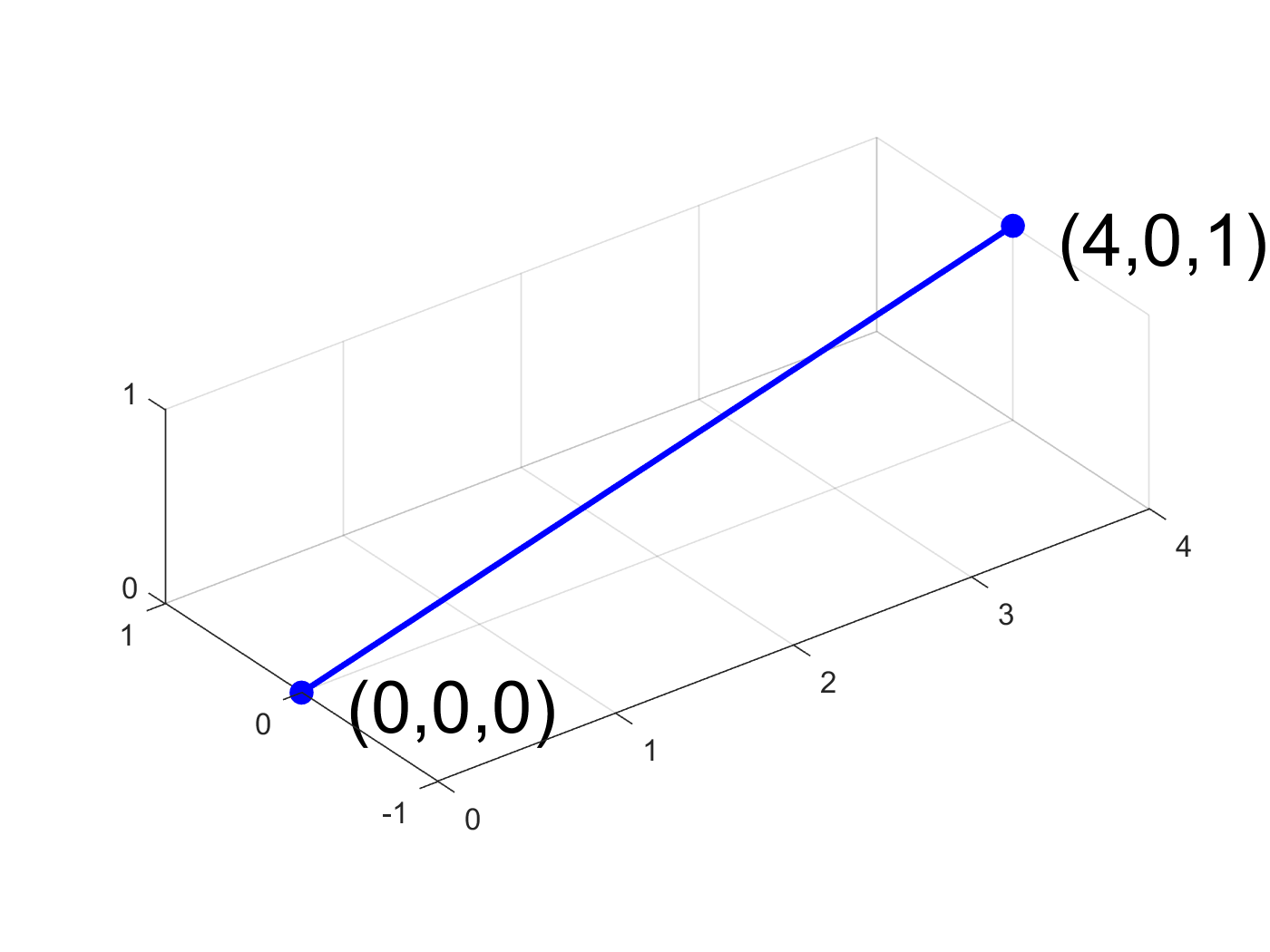
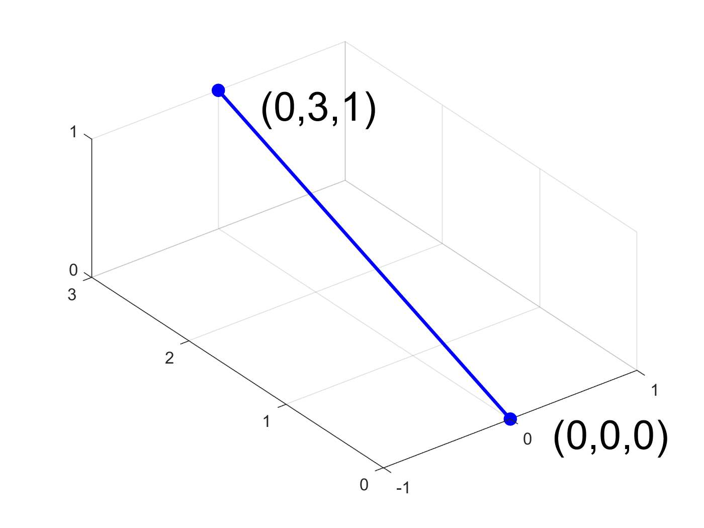
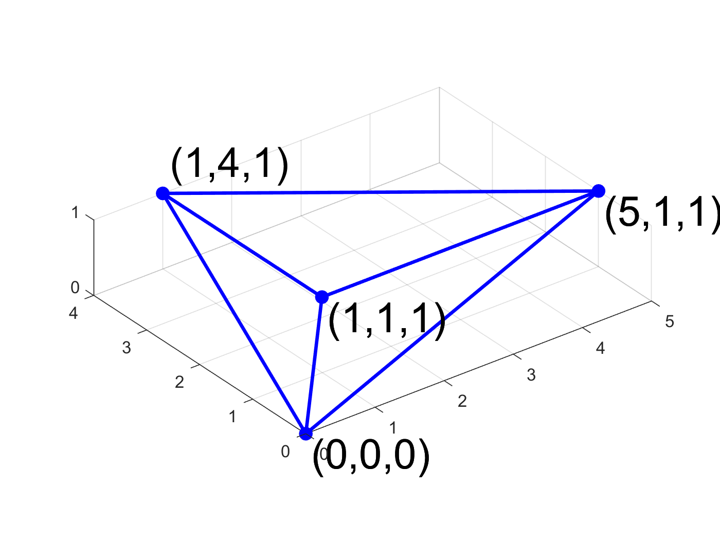
Figure 1. ${\mathrm{Newt}}(\ell_{1}),{\mathrm{Newt}}(\ell_{2})$ and ${\mathrm{Newt}}(\hat{\ell_{1}})={\mathrm{Newt}}(\hat{\ell_{2}})$ from Example 2.4

The following proposition shows that the assumption $x_{1}\cdots x_{n}\mid f_{j}$ for all $j\in[k]$ in Lemma 2.3 is not an issue.

Proposition 2.5.

Let $F=\langle f_{1},\ldots,f_{k}\rangle$ and $\hat{F}=\langle\hat{f}_{1},\ldots,\hat{f}_{k}\rangle$ where $f_{j}\in\mathbb{C}[x_{1},\ldots,x_{n}]$ and $\hat{f}_{j}=x_{1}\cdots x_{n}\cdot f_{j}$ for $j\in[k]$. The ML degree of $F$ equals the ML degree of $\hat{F}$.

Proof.

Recall the definition of ML system in (2.5), and let

$$\mathcal{L}(F)=\langle\ell_{1},\ldots,\ell_{n},f_{1},\ldots,f_{k}\rangle\text{ and }\mathcal{L}(\hat{F})=\langle\hat{\ell}_{1},\ldots,\hat{\ell}_{n},\hat{f}_{1},\ldots,\hat{f}_{k}\rangle.$$

By Proposition 2.1 it suffices to show that there is a bijection between $\mathcal{V}(\mathcal{L}(F))\cap(\mathbb{C}^{*})^{n+k}$ and $\mathcal{V}(\mathcal{L}(\hat{F}))\cap(\mathbb{C}^{*})^{n+k}$. We claim such a bijection is given by

$$\phi:\mathcal{V}(\mathcal{L}(F))\cap(\mathbb{C}^{*})^{n+k} \to\mathcal{V}(\mathcal{L}(\hat{F}))\cap(\mathbb{C}^{*})^{n+k}$$

$$(x_{1},\ldots,x_{n},\lambda_{1},\ldots,\lambda_{k}) \mapsto(x_{1},\ldots,x_{n},\frac{\lambda_{1}}{x_{1}\cdots x_{n}},\ldots,\frac{\lambda_{k}}{x_{1}\cdots x_{n}})$$

We need to show that $\phi$ is well defined. Since we assume $(x,\lambda)\in(\mathbb{C}^{*})^{n+k}$, $\frac{\lambda_{i}}{x_{1}\cdots x_{n}}$ is well defined. Now observe that if $f_{j}(x_{1},\ldots,x_{n})=0$ then $\hat{f}_{j}=x_{1}\cdots x_{n}\cdot f_{j}(x_{1},\ldots,x_{n})=0$ so we only need to show $\hat{\ell}_{i}$ vanishes on the image of $\phi$. By definition,

$$\hat{\ell}_{i} =u_{i}-x_{i}\cdot\sum_{j=1}^{k}\lambda_{j}\frac{\partial}{\partial x_{i}}(x_{1}\cdots x_{n}f_{j})$$

$$=u_{i}-x_{i}\cdot\sum_{j=1}^{k}\lambda_{j}(x_{1}\cdots x_{i-1}x_{i+1}\cdots x_{n}f_{j}+x_{1}\cdots x_{n}\frac{\partial}{\partial x_{i}}(f_{j})).$$

Since $f_{j}(x_{1},\ldots,x_{n})=0$ the first term in the summand vanishes. Substituting $\lambda_{j}\mapsto\frac{\lambda_{j}}{x_{1}\cdots x_{n}}$, the result is then clear.

Consider

$$\phi^{-1}:\mathcal{V}(\mathcal{L}(F))\cap(\mathbb{C}^{*})^{n+k} \to\mathcal{V}(\mathcal{L}(\hat{F}))\cap(\mathbb{C}^{*})^{n+k}$$

$$(x_{1},\ldots,x_{n},\lambda_{1},\ldots,\lambda_{k}) \mapsto(x_{1},\ldots,x_{n},x_{1}\cdots x_{n}\lambda_{1},\ldots,x_{1}\cdots x_{n}\lambda_{k}).$$

It is clear that the map $\phi\circ\phi^{-1}=\phi^{-1}\circ\phi$ is the identity, and that

$$\phi^{-1}(x_{1},\ldots,x_{n},\lambda_{1},\ldots,\lambda_{k})\in\mathcal{V}(\mathcal{L}(F))\cap(\mathbb{C}^{*})^{n+k}.$$

∎

2.2. Initial systems of the likelihood equations

We now consider the geometry of the Newton polytopes of the likelihood equations and how it relates to the number of $\mathbb{C}^{*}$ solutions to these equations.

Given a nonzero vector $w\in\mathbb{Z}^{n}$ and a polytope $P\subseteq\mathbb{R}^{n}$, we denote $P_{w}$ as the face exposed by $w$ and ${\mathrm{val}}_{w}(P)$ the value $w$ takes on this face. Specifically:

$$P_{w}=\{x\in P:\langle w,x\rangle\leq\langle w,y\rangle\ \text{ for all }\ y\in P\}\quad\text{and }\quad{\mathrm{val}}_{w}(P)=\min_{x\in P}\langle w,x\rangle,$$

with $\langle(w_{1},\dots,w_{n}),(x_{1},\dots,x_{n})\rangle:=w_{1}x_{1}+\cdots w_{n}x_{n}$. If $f=\sum_{\alpha\in{\mathrm{Newt}}(f)}c_{\alpha}x^{\alpha}$, we call

$${\mathrm{init}}_{w}(f)=\sum_{\alpha\in({\mathrm{Newt}}(f))_{w}}c_{\alpha}x^{\alpha}$$

the initial polynomial of $f$. For convenience, let ${\mathrm{Newt}}_{w}(f)$ denote $({\mathrm{Newt}}(f))_{w}$ and ${\mathrm{val}}_{w}(f)={\mathrm{val}}_{w}({\mathrm{Newt}}(f))$. For more background on initial polynomials, see [15, Chapter 2].

For convex bodies $K_{1},\dots,K_{n}$ in $\mathbb{R}^{n}$, consider the Minkowski sum $\mu_{1}K_{1}+\cdots+\mu_{n}K_{n}.$ The volume of $\mu_{1}K_{1}+\cdots+\mu_{n}K_{n}$ as a function of $\mu_{1},\dots,\mu_{n}$ is a homogeneous polynomial $Q(\mu_{1},\dots,\mu_{n})$ of degree $n$. The mixed volume of $K_{1},\dots,K_{n}$, denoted ${\mathrm{MVol}}(K_{1},\ldots,K_{n})$, is defined to be the coefficient of $\mu_{1}\cdots\mu_{n}$ in $Q$. For more details about mixed volumes see [20].

There are three important properties of the mixed volume which we wish to highlight:

1. Translation Invariance: ${\mathrm{MVol}}(K_{1},\ldots,K_{n})={\mathrm{MVol}}(a+K_{1},\ldots,K_{n})$ for $a\in\mathbb{R}^{n}$,

2. Monotonicity: ${\mathrm{MVol}}(\tilde{K}_{1},K_{2}\ldots,K_{n})\leq{\mathrm{MVol}}({K}_{1},\ldots,K_{n})$ when $\tilde{K}_{1}\subseteq{K}_{1}$,

3. Special Linear Invariance: ${\mathrm{MVol}}(K_{1},\ldots,K_{n})={\mathrm{MVol}}(\phi K_{1},\ldots,\phi K_{n})$ for any $\phi$ in the special linear group $\operatorname{SL}_{n}(\mathbb{R}$).

Recent work has analyzed when the monotonicity inequality is strict [7]. The connection between the convex geometry of a polynomial system and the number of $\mathbb{C}^{*}$ solutions to this system was made in a sequence of papers [6, 28, 29].

Theorem 2.6 (BKK bound ).

Let $G=\langle g_{1},\dots,g_{n}\rangle$ be a general sparse polynomial system in $\mathbb{C}[x_{1},\dots,x_{n}]$ and let $P_{1},\dots,P_{n}$ be their respective Newton polytopes. The number of $\mathbb{C}^{*}$-solutions to $F=0$ is equal to ${\mathrm{MVol}}(P_{1},\ldots,P_{n})$. Moreover, ${\mathrm{MVol}}(P_{1},\ldots,P_{n})$ is an upper bound for the number of isolated solutions in $(\mathbb{C}^{*})^{n}$ for a system with arbitrary coefficients. If for every nonzero $w\in\mathbb{Z}^{n}$, the initial systems ${\mathrm{init}}_{w}(g_{1},...,g_{n})$ have no solutions in $(\mathbb{C}^{*})^{n}$, then all the roots of the system are isolated.

By Proposition 2.1 we know that for a general sparse polynomial system $F$ and data vector $u$, there are finitely many complex solutions to the likelihood equations and that all such complex solutions live in the torus. Therefore, we would like to use Theorem 2.6 to identify the ML degree of $F$. To do this we need some preliminary results.

By Lemma 2.3, if $x_{1}\cdots x_{n}\mid f_{j}$ for all $j\in[k]$ then

$${\mathrm{Newt}}(\ell_{j})={\mathrm{Newt}}(\ell_{i})$$

for $i,j\in[n]$. Call this polytope $P$. Given some nonzero weight vector $w\in\mathbb{Z}^{n+k}$, we would like to determine which face of $P$ is exposed by $w$, based on which faces of ${\mathrm{Newt}}(f_{1}),\ldots,{\mathrm{Newt}}(f_{k})$ are exposed by $w$.

Lemma 2.7.

Let $F=\langle f_{1},\dots,f_{k}\rangle$ denote a general sparse polynomial system. Let $\tilde{e}_{j}\in\mathbb{R}^{n+k}$ be the vector with $(n+j)$-th entry equal to $1$ and all other entries equal to  $0$. Suppose $w$ is a nonzero weight vector in $\mathbb{Z}^{n+k}$.

If $x_{1}\cdots x_{n}\mid f_{j}$ for all $j\in[k]$, then up to reordering the $f_{1},\ldots,f_{k}$, $w$ exposes $P$ on one of the following faces:

1. the origin,

2. ${\mathrm{Conv}}(\tilde{e}_{1}+{\mathrm{Newt}}_{w}(f_{1}),\ldots,\tilde{e}_{t}+{\mathrm{Newt}}_{w}(f_{t}))$ for some $t\in[k]$,

3. ${\mathrm{Conv}}(0,\tilde{e}_{1}+{\mathrm{Newt}}_{w}(f_{1}),\ldots,\tilde{e}_{t}+{\mathrm{Newt}}_{w}(f_{t}))$ for some $t\in[k]$.

Proof.

Fix a nonzero weight vector $w=(a,b)\in\mathbb{R}^{n}\times\mathbb{R}^{k}$ and suppose $(v,0_{k})\in{\mathrm{Newt}}(f_{1})\setminus{\mathrm{Newt}}_{w}(f_{1})$. From the description of $P$ in Lemma 2.3 we have that

$${\mathrm{val}}_{w}(P)\in\{0,b_{1}+{\mathrm{val}}_{w}(f_{1}),\ldots,b_{k}+{\mathrm{val}}_{w}(f_{k})\}.$$

If $b_{j}+{\mathrm{val}}_{w}(f_{j})>0$ for all $j\in[k]$, then $P$ is exposed at the origin, so we are in Case 1. If $b_{1}+{\mathrm{val}}_{w}(f_{1})=\cdots=b_{t}+{\mathrm{val}}_{w}(f_{t})=\gamma<0$ for some $t\in[k]$, where $b_{j}+{\mathrm{val}}_{w}(f_{j})>\gamma$ for all $t+1\leq j\leq k$, then we are in Case 2. If above $\gamma=0$, then we are in Case 3. ∎

We illustrate Lemma 2.7 with the following example.

Example 2.8.

Recall the ML system $\mathcal{L}(\hat{f})$ from Example 2.4 where $\hat{f}=\langle xy(2x^{4}+3y^{3}-5)\rangle$ and $P$ from Figure 1. Consider the three weight vectors

$$w_{1}=(-3,14,3),\quad w_{2}=(-3,-4,3),\quad w_{3}=(-3,12,3).$$

The respective exposed faces of $P$ for these weight vectors are

$$P_{w_{1}}=\{(0,0,0)\},\quad P_{w_{2}}={\mathrm{Conv}}(\{(5,1,1),(1,4,1)\}),\quad P_{w_{3}}={\mathrm{Conv}}(\{(0,0,0),(5,1,1)\}),$$

and are shown in red in Figure 2. Each $P_{w_{i}}$ corresponds to one of the three cases in Lemma 2.7. Namely, $P_{w_{1}}$ is the origin; $P_{w_{2}}$ is in Case 2; and $P_{w_{3}}$ is in Case 3.

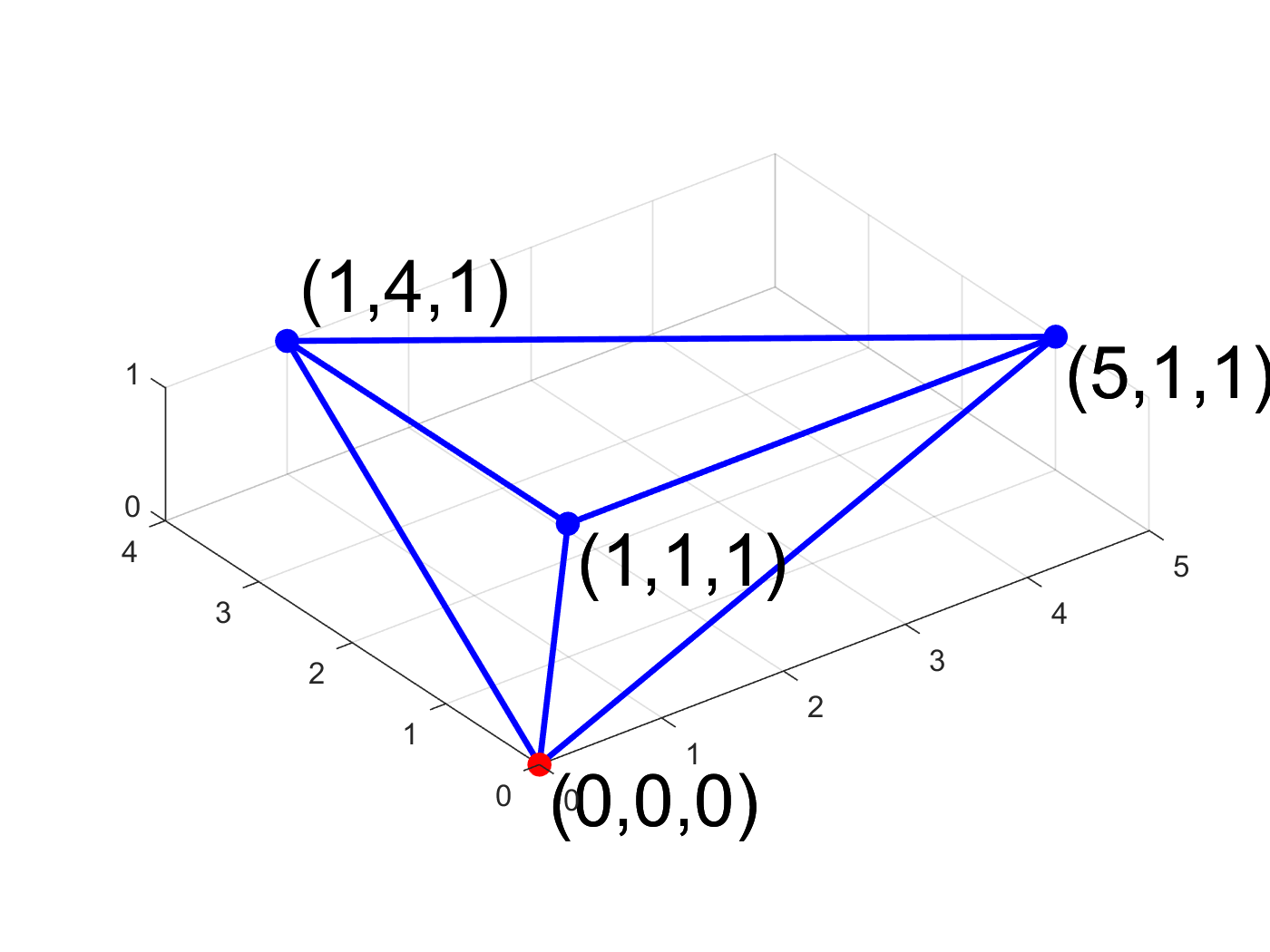
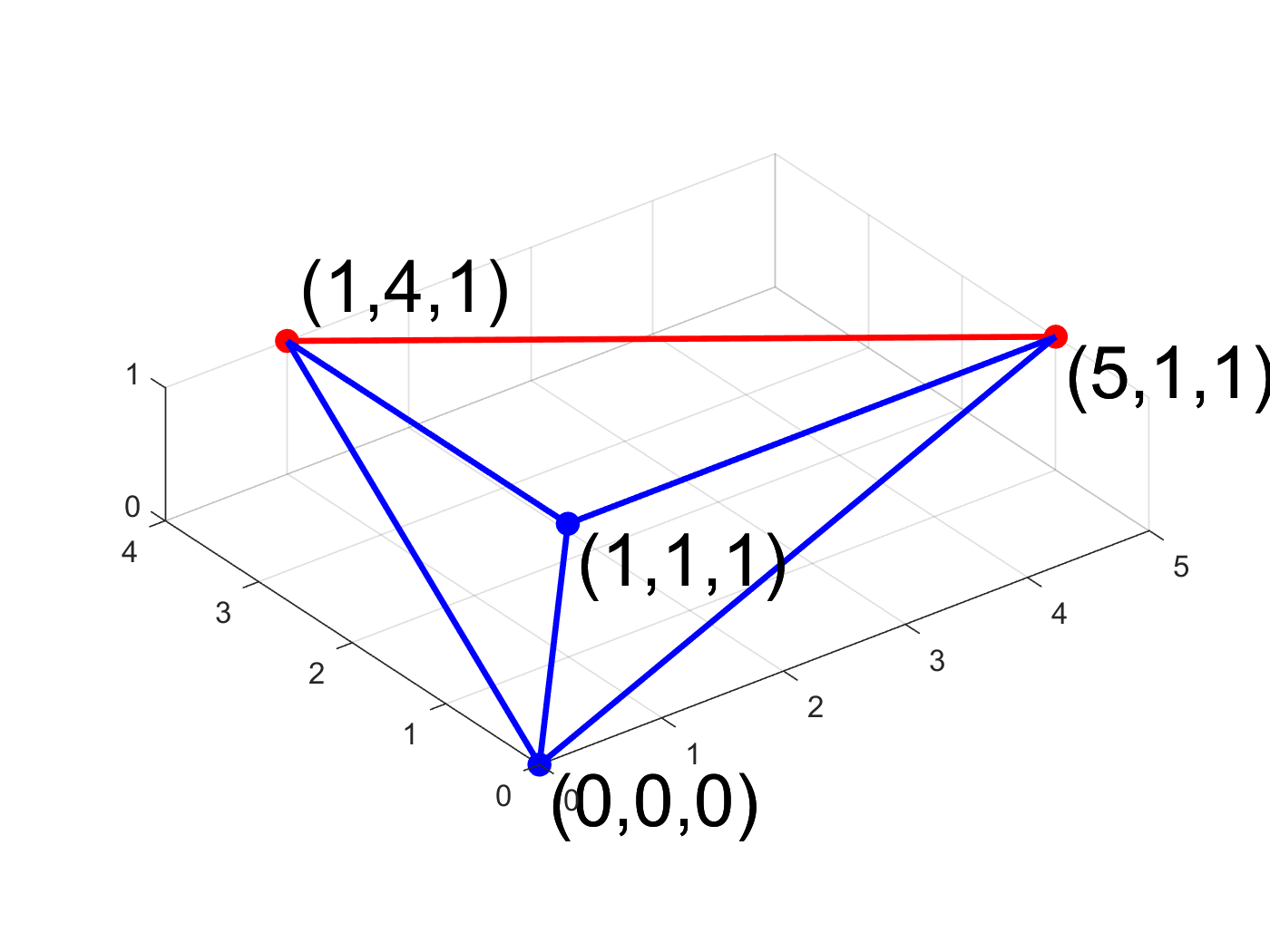
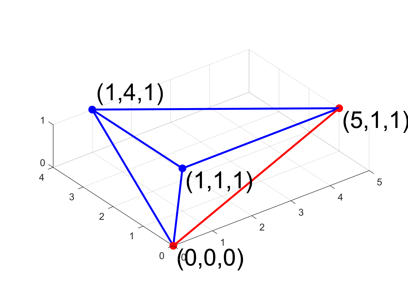
Figure 2. $P_{w_{1}},P_{w_{2}}$ and $P_{w_{3}}$ from Example 2.8.

We now need to show that for each of the three cases outlined in Lemma 2.7, there are no $\mathbb{C}^{*}$ solutions to the corresponding initial system.

Lemma 2.9.

Let $F=\langle f_{1},\dots,f_{k}\rangle$ denote a general sparse polynomial system. If $x_{1}\cdots x_{n}\mid f_{j}$ for all $j\in[k]$, then there are no $\mathbb{C}^{*}$ solutions to ${\mathrm{init}}_{w}(\mathcal{L}(F))$ when $P_{w}$ is as in Case 1.

Proof.

Recall that in Case 1 in Lemma 2.7, $P_{w}$ is the origin. In this case we have ${\mathrm{init}}_{w}(\ell_{i})=u_{i}=0$. Since generally $u_{i}\neq 0$, this initial system has no solutions. ∎

Lemma 2.10.

Let $F=\langle f_{1},\dots,f_{k}\rangle$ denote a general sparse polynomial system. If $x_{1}\cdots x_{n}\mid f_{j}$ for all $j\in[k]$, then there are no $\mathbb{C}^{*}$ solutions to ${\mathrm{init}}_{w}(\mathcal{L}(F))$ when $P_{w}$ is as in Case 2.

Proof.

Recall that in Case 2 in Lemma 2.7, $P_{w}$ is ${\mathrm{Conv}}(\tilde{e}_{1}+{\mathrm{Newt}}_{w}(f_{1}),\ldots,\tilde{e}_{t}+{\mathrm{Newt}}_{w}(f_{t}))$ for some $t\in[k]$.

Let $\tilde{f}_{j}={\mathrm{init}}_{w}(f_{j})$ for $j\in[k]$. We consider the following as a subsystem of ${\mathrm{init}}_{w}(\mathcal{L}(F))$:

$$\tilde{f_{1}} =\ldots=\tilde{f_{t}}=0,$$

$$x_{1}\big{(}\sum_{j=1}^{t}\lambda_{j}\frac{\partial}{\partial x_{1}}(\tilde{f_{j}})\Big{)} =\ldots=x_{n}\big{(}\sum_{j=1}^{t}\lambda_{j}\frac{\partial}{\partial x_{n}}(\tilde{f}_{j})\Big{)}=0.$$

Since we only consider $\mathbb{C}^{*}$ solutions, this reduces to

$$\tilde{f_{1}} =\ldots=\tilde{f_{t}}=0,$$

$$\sum_{j=1}^{t}\lambda_{j}\frac{\partial}{\partial x_{1}}(\tilde{f_{j}}) =\ldots=\sum_{j=1}^{t}\lambda_{j}\frac{\partial}{\partial x_{n}}(\tilde{f_{j}})=0.$$

By Bertini's Theorem [23, Ch. III,§10.9.2], the variety cut out by $\tilde{f}_{1}=0,\ldots,\tilde{f}_{t}=0$ has codimension $t$ in $(\mathbb{C}^{*})^{n}$ and $\mathcal{V}(\tilde{f}_{1},\ldots,\tilde{f}_{t})$ has no singular solutions in the torus. So this initial system has no $\mathbb{C}^{*}$ solutions.

∎

Before we consider the final case of Lemma 2.7, we need a preliminary lemma.

Lemma 2.11.

Let $F=\langle f_{1},\dots,f_{k}\rangle$ denote a general sparse polynomial system where $x_{1}\cdots x_{n}\mid f_{j}$ for all $j\in[k]$. Furthermore, let $w=(a,b)\in\mathbb{Z}^{n}\times\mathbb{Z}^{k}$ be a nonzero weight vector. If $a=0$ then there are no $\mathbb{C}^{*}$ solutions to ${\mathrm{init}}_{w}(\mathcal{L}(F))$.

Proof.

Under the assumption $a=0$,

$${\mathrm{Newt}}_{w}(f_{j})={\mathrm{Newt}}(f_{j})\text{ and }{\mathrm{val}}_{w}(f_{j})=0\text{ for all }j\in[k].$$

Recall from the proof of Lemma 2.7,

$${\mathrm{val}}_{w}(P)\in\{0,b_{1}+{\mathrm{val}}_{w}(f_{1}),\ldots,b_{k}+{\mathrm{val}}_{w}(f_{k})\}.$$

Since ${\mathrm{val}}_{w}(f_{j})=0$, this gives that ${\mathrm{val}}_{w}(P)\in\{0,b_{1},\ldots,b_{k}\}$. If any $b_{j}<0$ or all $b_{j}>0$ for $j\in[k]$, then by Lemmas 2.10 and 2.9 there are no $\mathbb{C}^{*}$ solutions to the initial system.

It remains to consider when

$$b_{1}=\ldots=b_{t}=0\ \text{ and }\ b_{t+1},\ldots,b_{k}>0.$$

Note that $t<k$, because otherwise $b$ would be the all zeros vector, which is not allowed. Observe that ${\mathrm{init}}_{w}(\ell_{1},\ldots,\ell_{n},f_{1},\ldots,f_{t})$ is equal to the ML system of $(f_{1},\ldots,f_{t})$. By Proposition 2.1 there are finitely many solutions to this ML system. Since $f_{t+1},\ldots,f_{k}$ are general, their respective hypersurfaces do not intersect the variety of this Lagrange system. ∎

Lemma 2.12.

Let $F=\langle f_{1},\dots,f_{k}\rangle$ denote a general sparse polynomial system. If $x_{1}\cdots x_{n}\mid f_{j}$ for all $j\in[k]$, then there are no $\mathbb{C}^{*}$ solutions to ${\mathrm{init}}_{w}(\mathcal{L}(F))$ when $P_{w}$ is as in Case 3.

Proof.

Recall from Case 3 in Lemma 2.7, $P_{w}$ is ${\mathrm{Conv}}(0,\tilde{e}_{1}+{\mathrm{Newt}}_{w}(f_{1}),\ldots,\tilde{e}_{t}+{\mathrm{Newt}}_{w}(f_{t}))$ for some $t\in[k]$. Let $\tilde{f}_{j}={\mathrm{init}}_{w}(f_{j})$ for $j\in[k]$.

We consider the subsystem of ${\mathrm{init}}_{w}(\mathcal{L}(F))$ given by:

$$\tilde{f_{1}}=\ldots=\tilde{f_{t}} =0$$

$$x_{1}\sum_{j=1}^{t}\lambda_{j}\frac{\partial}{\partial x_{1}}(\tilde{f_{j}}) =u_{1}$$

$$\vdots\qquad$$

$$x_{n}\sum_{j=1}^{t}\lambda_{j}\frac{\partial}{\partial x_{n}}(\tilde{f_{j}}) =u_{n}.$$

Multiplying $\tilde{f}_{j}$ by $\lambda_{j}$, this becomes

$$\lambda_{1}\tilde{f_{1}}=\ldots=\lambda_{t}\tilde{f_{t}} =0$$

$$x_{1}\sum_{j=1}^{t}\lambda_{j}\frac{\partial}{\partial x_{1}}(\tilde{f_{j}}) =u_{1}$$

$$\vdots\qquad$$

$$x_{n}\sum_{j=1}^{t}\lambda_{j}\frac{\partial}{\partial x_{n}}(\tilde{f_{j}}) =u_{n}.$$

Observe that $\lambda_{j}\tilde{f}_{j}$ has the same monomial support as $x_{i}\lambda_{j}\frac{\partial}{\partial x_{i}}(\tilde{f}_{j})$ for all $i\in[n]$. Therefore if we write $\lambda_{j}\tilde{f}_{j}=\sum_{i=1}^{M_{j}}c_{i,j}x^{\alpha_{i,j}}$ we can write ${\mathrm{init}}_{w}(\ell_{1},\ldots,\ell_{n},f_{1},\ldots,f_{t})$ as the linear system $AX=U$:

$$\begin{bmatrix}\vline&&\vline&&\vline&&\vline&&\\ \alpha_{1,1}&\ldots&\alpha_{1,M_{1}}&\ldots&\alpha_{t,1}&\ldots&\alpha_{t,M_{t}}\\ \vline&&\vline&&\vline&&\vline\\ -&\mathbf{1}_{M_{1}}&-&&0&\cdots&0\\ &\vdots&&&\vdots&&\vdots\\ 0&\cdots&0&\cdots&-&\mathbf{1}_{M_{t}}&-\end{bmatrix}\cdot\begin{bmatrix}c_{1,1}x^{\alpha_{1,1}}\\ \vdots\\ c_{1,M_{1}}x^{\alpha,M_{1}}\\ \vdots\\ c_{t,1}x^{\alpha_{t},1}\\ \vdots\\ c_{t,M_{t}}x^{\alpha_{t,M_{t}}}\end{bmatrix} =\begin{bmatrix}u_{1}\\ \vdots\\ u_{n}\\ 0\\ \vdots\\ 0\end{bmatrix}.$$

Note that $A\in\mathbb{N}^{(n+t)\times(M_{1}+\ldots+M_{t})}$, $X\in\mathbb{R}^{M_{1}+\ldots+M_{t}}$, $U\in\mathbb{N}^{n+t}$, and $\mathbf{1}_{M_{i}}$ is a row vector of size $M_{i}$ of all ones.

For $M_{1},\dots,M_{t}$ large enough, a dimension count of $A$ suggests its rows are linearly independent. However, it turns out that no matter the size of $M_{1},\dots,M_{t}$, the matrix $A$ always has a nontrivial left kernel vector:

$$(a_{1},\ldots,a_{n},-{\mathrm{val}}_{w}(f_{1}),\ldots,-{\mathrm{val}}_{w}(f_{t})),$$

where $w=(a,b)\in\mathbb{Z}^{n}\times\mathbb{Z}^{k}$. This follows from $\langle a,\alpha_{j,i}\rangle={\mathrm{val}}_{w}(f_{j})$ for $j\in[t]$.

By Lemma 2.11, we know that some of the $a_{i}$ are nonzero, which contradicts the generality of $u$, as it would imply that $\langle a,u\rangle=0$ with $a\neq 0$.

∎

2.3. Main result and consequences

Theorem 2.13 (Main Result).

For general sparse polynomials $F=\langle f_{1},\dots,f_{k}\rangle$, denote its ML system $\eqref{eq:MLsystem}$ by $\mathcal{L}(F)$. The ML degree of $F$ equals the mixed volume of $\mathcal{L}(F)$.

Proof.

For readability, we abbreviate ${\mathrm{MVol}}({\mathrm{Newt}}(g_{1}),\dots,{\mathrm{Newt}}(g_{n}))$ by ${\mathrm{MVol}}(g_{1},\dots,g_{n})$ throughout the proof. Consider the system $\hat{F}=(\hat{f}_{1},\ldots,\hat{f}_{k})$ where $\hat{f}_{j}=x_{1}\cdots x_{n}\cdot f_{j}$ for $j\in~{}[k]$. It follows from Theorem 2.6, Proposition 2.1 and Lemmas 2.7, 2.9,  2.10 and 2.12 that the ML degree of $\hat{F}$ equals the mixed volume of $\mathcal{L}(\hat{F})$.

Now we show that the ML degree of $F$ equals the mixed volume of $\mathcal{L}(F)$. First observe that ${\mathrm{Newt}}(f_{j})+(\mathbf{1}_{n},0_{k})={\mathrm{Newt}}(\hat{f}_{j})$ for $j\in[k]$. Since the mixed volume is translation invariant, this gives

$${\mathrm{MVol}}(\ell_{1},\ldots,\ell_{n},f_{1},\ldots,f_{k})={\mathrm{MVol}}(\ell_{1},\ldots,\ell_{n},\hat{f}_{1},\ldots,\hat{f}_{k}).$$

For $\phi\in\operatorname{SL}_{n+k}$ given by

$$\begin{bmatrix}I_{n}&\mathbf{1}_{n\times k}\\ 0_{k\times n}&I_{k}\end{bmatrix},$$

we have

$${\mathrm{MVol}}(\ell_{1},\ldots,\ell_{n},\hat{f}_{1},\ldots,\hat{f}_{k}) ={\mathrm{MVol}}(\phi\cdot\ell_{1},\ldots,\phi\cdot\ell_{n},\phi\cdot\hat{f}_{1},\ldots,\phi\cdot\hat{f}_{k})$$

$$={\mathrm{MVol}}(\phi\cdot\ell_{1},\ldots,\phi\cdot\ell_{n},\hat{f}_{1},\ldots,\hat{f}_{k}).$$

Since $\phi({\mathrm{Newt}}(\ell_{i}))\subseteq{\mathrm{Newt}}(\hat{\ell}_{i})$, by monotonicity of mixed volume we get

$${\mathrm{MVol}}(\phi\cdot\ell_{1},\ldots,\phi\cdot\ell_{n},\hat{f}_{1},\ldots,\hat{f}_{k})\leq{\mathrm{MVol}}(\hat{\ell}_{1},\ldots,\hat{\ell}_{n},\hat{f}_{1},\ldots,\hat{f}_{k}).$$

Thus far we have shown the inequality ${\mathrm{MVol}}(\mathcal{L}(F))\leq{\mathrm{MVol}}(\mathcal{L}(\hat{F}))$. We claim the following list of equalities also holds:

(2.6) $${\mathrm{MVol}}(\mathcal{L}(\hat{F}))\,\,=\,\,\text{ML Degree of }\hat{F}\,\,=\,\,\text{ML Degree of }F\,\,\leq\,\,{\mathrm{MVol}}(\mathcal{L}(F)).$$

From the argument given above we also have that the mixed volume of $\mathcal{L}(\hat{F})$ is equal to the ML degree of $\hat{F}$. By Proposition 2.5 we have that the ML degree of $\hat{F}$ equals the ML degree of $F$. The first part of Theorem 2.6 tells us that the ML degree of $F$ is upper bounded by the mixed volume of $\mathcal{L}(F)$. The inequalitiy ${\mathrm{MVol}}(\mathcal{L}(F))\leq{\mathrm{MVol}}(\mathcal{L}(\hat{F}))$ paired with (2.6) shows that the mixed volume $\mathcal{L}(F)$ equals the ML degree of $F$. ∎

Remark 2.14.

Theorem 2.13 shows that an optimal homotopy method to find all critical points for maximum likelihood estimation is given by a standard polyhedral homotopy from its ML system. The polyhedral homotopy was presented in [26], and there exists off the shelf software implementations [10, 40, 31]. For the background in homotopy methods in numerical algebraic geometry see [5].

Remark 2.15 (Sum-to-one-constraint).

For MLE, typically $f_{1}\in F$ will be $x_{1}+\ldots+x_{n}-1$. Although this polynomial does not have general coefficients, we can rescale the variables so the traditional MLE situation falls into our set-up.

A corollary of our results is that the ML degree of a general sparse polynomial system $F$ depends only on the Newton polytopes.

Corollary 2.16.

Consider two general sparse polynomial systems: $F=\langle f_{1},\ldots,f_{k}\rangle$ and $G=\langle g_{1},\ldots,g_{k}\rangle$, where ${\mathrm{Newt}}(f_{j})={\mathrm{Newt}}(g_{j})$ for $j\in[k]$. The ML degree of $F$ equals the ML degree of $G$.

Proof.

Suppose $F$ and $G$ have the same Newton polytopes. Consider $x_{1}\cdots x_{n}F=\hat{F}$ and $x_{1}\cdots x_{n}G=\hat{G}$. The ML systems of $\hat{F}$ and $\hat{G}$ have the same Newton polytopes, so by Theorem 2.13 the ML degree of $\hat{F}$ equals the ML degree of $\hat{G}$. Proposition 2.5 then gives that the ML degree of $F$ equals the ML degree of $\hat{F}$ and likewise for $G$ and $\hat{G}$, giving the result. ∎

This is a surprising corollary because the Newton polytopes of $F$ do not determine the Newton polytopes of the respective ML system.

Example 2.17.

Consider the ML systems $\mathcal{L}(f)$ and $\mathcal{L}(\hat{f})$ from Example 2.4 and Example 2.8. Both of these systems have a mixed volume and ML degree equal to $12$ even though the Newton polytopes of the corresponding ML systems are quite different.

References

- [1] P. Aluffi and C. Harris. The Euclidean distance degree of smooth complex projective varieties. Algebra Number Theory, 12(8):2005–2032, 2018.
- [2] C. Améndola, N. Bliss, I. Burke, C. R. Gibbons, M. Helmer, S. Hoşten, E. D. Nash, J. I. Rodriguez, and D. Smolkin. The maximum likelihood degree of toric varieties. J. Symbolic Comput., 92:222–242, 2019.
- [3] C. Améndola, K. Kohn, P. Reichenbach, and A. Seigal. Invariant theory and scaling algorithms for maximum likelihood estimation. SIAM J. Appl. Algebra Geom., 5(2):304–337, 2021.
- [4] J. A. Baaijens and J. Draisma. Euclidean distance degrees of real algebraic groups. Linear Algebra Appl., 467:174–187, 2015.
- [5] D. J. Bates, J. D. Hauenstein, A. J. Sommese, and C. W. Wampler. Numerically solving polynomial systems with Bertini, volume 25 of Software, Environments, and Tools. Society for Industrial and Applied Mathematics (SIAM), Philadelphia, PA, 2013.
- [6] D. N. Bernstein. The number of roots of a system of equations. Funkcional. Anal. i Priložen., 9(3):1–4, 1975.
- [7] F. Bihan and I. Soprunov. Criteria for strict monotonicity of the mixed volume of convex polytopes. Adv. Geom., 19(4):527–540, 2019.
- [8] G. Blekherman, P. A. Parrilo, and R. R. Thomas, editors. Semidefinite optimization and convex algebraic geometry, volume 13 of MOS-SIAM Series on Optimization. Society for Industrial and Applied Mathematics (SIAM), Philadelphia, PA; Mathematical Optimization Society, Philadelphia, PA, 2013.
- [9] P. Breiding, F. Sottile, and J. Woodcock. Euclidean distance degree and mixed volume. arXiv preprint arXiv:2012.06350, 2020.
- [10] P. Breiding and S. Timme. Homotopycontinuation.jl: A package for homotopy continuation in Julia. In Mathematical Software – ICMS 2018, pages 458–465. Springer International Publishing, 2018.
- [11] T. Brysiewicz, J. I. Rodriguez, F. Sottile, and T. Yahl. Solving decomposable sparse systems. Numer. Algorithms, 88(1):453–474, 2021.
- [12] F. Catanese, S. Hoşten, A. Khetan, and B. Sturmfels. The maximum likelihood degree. Amer. J. Math., 128(3):671–697, 2006.
- [13] D. Cifuentes, C. Harris, and B. Sturmfels. The geometry of SDP-exactness in quadratic optimization. Math. Program., 182(1-2, Ser. A):399–428, 2020.
- [14] P. Clarke and D. A. Cox. Moment maps, strict linear precision, and maximum likelihood degree one. Adv. Math., 370:107233, 51, 2020.
- [15] D. A. Cox, J. Little, and D. O'Shea. Ideals, varieties, and algorithms. Undergraduate Texts in Mathematics. Springer, Cham, fourth edition, 2015. An introduction to computational algebraic geometry and commutative algebra.
- [16] H. Derksen and V. Makam. Maximum likelihood estimation for matrix normal models via quiver representations. SIAM J. Appl. Algebra Geom., 5(2):338–365, 2021.
- [17] J. Draisma, E. Horobeţ, G. Ottaviani, B. Sturmfels, and R. Thomas. The Euclidean distance degree. In SNC 2014—Proceedings of the 2014 Symposium on Symbolic-Numeric Computation, pages 9–16. ACM, New York, 2014.
- [18] J. Draisma, E. Horobeţ, G. Ottaviani, B. Sturmfels, and R. R. Thomas. The Euclidean distance degree of an algebraic variety. Found. Comput. Math., 16(1):99–149, 2016.
- [19] D. Drusvyatskiy, H.-L. Lee, G. Ottaviani, and R. R. Thomas. The Euclidean distance degree of orthogonally invariant matrix varieties. Israel J. Math., 221(1):291–316, 2017.
- [20] G. Ewald. Combinatorial convexity and algebraic geometry, volume 168 of Graduate Texts in Mathematics. Springer-Verlag, New York, 1996.
- [21] H.-C. Graf von Bothmer and K. Ranestad. A general formula for the algebraic degree in semidefinite programming. Bull. Lond. Math. Soc., 41(2):193–197, 2009.
- [22] E. Gross, M. Drton, and S. Petrović. Maximum likelihood degree of variance component models. Electron. J. Stat., 6:993–1016, 2012.
- [23] R. Hartshorne. Algebraic geometry. Springer-Verlag, New York-Heidelberg, 1977. Graduate Texts in Mathematics, No. 52.
- [24] S. Hoşten, A. Khetan, and B. Sturmfels. Solving the likelihood equations. Found. Comput. Math., 5(4):389–407, 2005.
- [25] B. Huber and B. Sturmfels. A polyhedral method for solving sparse polynomial systems. Math. Comp., 64(212):1541–1555, 1995.
- [26] B. Huber and B. Sturmfels. A polyhedral method for solving sparse polynomial systems. Math. Comp., 64(212):1541–1555, 1995.
- [27] J. Huh. The maximum likelihood degree of a very affine variety. Compos. Math., 149(8):1245–1266, 2013.
- [28] A. G. Khovanskii. Newton polyhedra, and the genus of complete intersections. Funktsional. Anal. i Prilozhen., 12(1):51–61, 1978.
- [29] A. G. Kouchnirenko. Polyèdres de Newton et nombres de Milnor. Invent. Math., 32(1):1–31, 1976.
- [30] H. Lee. The Euclidean distance degree of Fermat hypersurfaces. J. Symbolic Comput., 80(part 2):502–510, 2017.
- [31] T. L. Lee, T. Y. Li, and C. H. Tsai. HOM4PS-2.0: a software package for solving polynomial systems by the polyhedral homotopy continuation method. Computing, 83(2-3):109–133, 2008.
- [32] L. G. Maxim, J. I. Rodriguez, and B. Wang. Defect of Euclidean distance degree. Adv. in Appl. Math., 121:102101, 22, 2020.
- [33] L. G. Maxim, J. I. Rodriguez, and B. Wang. Euclidean distance degree of the multiview variety. SIAM J. Appl. Algebra Geom., 4(1):28–48, 2020.
- [34] M. Michał ek, L. Monin, and J. a. A. Wiśniewski. Maximum likelihood degree, complete quadrics, and -action. SIAM J. Appl. Algebra Geom., 5(1):60–85, 2021.
- [35] J. Nie and K. Ranestad. Algebraic degree of polynomial optimization. SIAM J. Optim., 20(1):485–502, 2009.
- [36] J. Nie, K. Ranestad, and B. Sturmfels. The algebraic degree of semidefinite programming. Math. Program., 122(2, Ser. A):379–405, 2010.
- [37] J. I. Rodriguez and B. Wang. The maximum likelihood degree of mixtures of independence models. SIAM J. Appl. Algebra Geom., 1(1):484–506, 2017.
- [38] B. Sturmfels. Solving systems of polynomial equations, volume 97 of CBMS Regional Conference Series in Mathematics. Published for the Conference Board of the Mathematical Sciences, Washington, DC; by the American Mathematical Society, Providence, RI, 2002.
- [39] B. Sturmfels, S. Timme, and P. Zwiernik. Estimating linear covariance models with numerical nonlinear algebra. Algebr. Stat., 11(1):31–52, 2020.
- [40] J. Verschelde. Algorithm 795: Phcpack: a general-purpose solver for polynomial systems by homotopy continuation. ACM Transactions on Mathematical Software, 25(2):251–276, 1999.
- [41] J. Verschelde, P. Verlinden, and R. Cools. Homotopies exploiting Newton polytopes for solving sparse polynomial systems. SIAM J. Numer. Anal., 31(3):915–930, 1994.