Uniform Inference on High-dimensional Spatial Panel Networks

Abstract

We propose employing a debiased-regularized, high-dimensional generalized method of moments (GMM) framework to perform inference on large-scale spatial panel networks. In particular, network structure with a flexible sparse deviation, which can be regarded either as latent or as misspecified from a predetermined adjacency matrix, is estimated using debiased machine learning approach. The theoretical analysis establishes the consistency and asymptotic normality of our proposed estimator, taking into account general temporal and spatial dependency inherent in the data-generating processes. The dimensionality allowance in presence of dependency is discussed. A primary contribution of our study is the development of uniform inference theory that enables hypothesis testing on the parameters of interest, including zero or non-zero elements in the network structure. Additionally, the asymptotic properties for the estimator are derived for both linear and nonlinear moments. Simulations demonstrate superior performance of our proposed approach. Lastly, we apply our methodology to investigate the spatial network effect of stock returns.

Keywords: GMM, debiased machine learning, network analysis, high-dimensional time series, spatial panel data

1 Introduction

Network analysis has gained significant interest recently. In particular, measuring the connectedness in a complex system has become a central task in learning networks. Various forms of regressions with dependent variables affected by the outcomes and characteristics of network members are formulated for that purpose. The celebrated literature on social network analysis favors using a predetermined network structure, which is fully characterized by a specified adjacency matrix, to study peer effects in social networks; see for example Lee, (2007); Bramoullé et al., (2009); Lee et al., (2010); Yang and Lee, (2017); Zhu et al., (2020). As for spatial panel networks, Kuersteiner and Prucha, (2020) consider a class of GMM estimators for general dynamic panel models that allow for potential endogeneity and cross-sectional dependence. An alternative of imposing a known network structure is to estimate the adjacency matrix provided that the structural parameters are already identified. Examples of related studies include Blume et al., (2015); de Paula et al., (2019); Lewbel et al., 2023c .

With the rise of big data availability, many applications are concerned with large-scale networks consist of a large number of individuals. In particular, spatial panel data involving high-dimensional time series are observed in many financial and economic network analysis. This would pose the challenge of estimating too many unknown parameters. To reduce the dimensionality, various machine learning methods based on sparsity and penalization are employed to shrink the parameters. Manresa, (2016) use LASSO (Least Absolute Shrinkage and Selection Operator) to quantify the spillover effects in social network, where the endogenous interactions are not taken into consideration. de Paula et al., (2019) apply Adaptive Elastic Net GMM to estimate the interaction model with important contributions to the identification of the structural parameters. Ata et al., (2023) consider a reduced-form estimation with the innovative discovery of the algebraic results on how the sparsity of the structural parameters relates to that of the parameters in the reduced form. Lam and Souza, (2020) study the penalized estimation of spatial weight matrix through adaptive LASSO and show the oracle properties of the sparse estimator.

The machine learning methods seem notably effective in prediction performance. However, the statistical inference might be subject to substantial bias due to omitted variables. Debiasing is required in order to construct high quality point and interval estimates. Taking the LASSO-type methodology as example, Lam and Souza, (2020) establish the asymptotic normality for the non-zero elements in the network structure. In general, we do not have such prior information on whether the parameters are truly non-zero. Thus, uniform inference theory that enables testing on any parameters of interest is demanded. For the case of i.i.d. data, there are extensive studies that contribute in the issue of uniform inference under high-dimensional regression setting with exogeneity conditions (e.g., Belloni et al., (2014); Zhang and Zhang, (2014); Belloni et al., (2015); Chernozhukov et al., (2018)), and more generally those that consider a GMM setup allowing for endogeneity (e.g., Belloni et al., (2017, 2018); Caner and Kock, (2018)), with various forms of de-biased/orthogonalization methods. Based on the idea of orthogonality, Ata et al., (2023) present an algorithm incorporating bias-corrected Dantzig selector estimator to investigate large networks in presence of latent agents, albeit without accounting for time dependence. Concerning data-generating processes exhibiting dependency, Chernozhukov et al., (2021) study the LASSO-driven inference for exogenous regression with general temporal and cross-sectional dependent data.

In this paper, we are motivated to understand the connectedness in a complex spatial panel network. In particular, our focus is on exploring network structures (not necessary to be sparse) with a flexible sparse deviation, which can be regarded either as latent or as misspecified from a predetermined adjacency matrix (e.g. credit chain or common ownership information in a financial system). Specifically, we target network formation and formulate the problem into a general system of dynamic regression equations, taking into account general temporal and spatial dependency inherent in the data-generating processes. Methodologically, we extend the model setting in Chernozhukov et al., (2021) by allowing for endogeneity in the covariates, which is a natural concern when the regression system is featured with simultaneity by incorporating contemporaneous lags. As a result, sufficiently many moment conditions involving instrument variables are needed and we build a debiased-regularized, high-dimensional GMM framework to facilitate valid inference.

For implementation, we propose using a Generalized Dantzig Selector followed by a debiasing step. Theoretically, we derive the consistency and linearize the estimator for a proper application of the central limit theorem for uniform inference on the parameters of interest (of either fixed or growing dimension). The dimensionality allowance in presence of dependency is discussed. In particular, we show the asymptotic properties of the debiased-regularized GMM (DRGMM) estimator in the case of linear or nonlinear moments, respectively. Moreover, we discuss the link to the semiparametric efficiency literature regarding the construction of our estimator when the dimension of the parameters of interest is fixed.

We contribute to the literature in four respects. First, we develop a method to estimate parameters in a high-dimensional endogenous equation system with incorporating dynamics in both spatial and temporal. Our theoretical framework accords with general dynamic panel models, with heterogeneity reflected in the individual-based parameters. Second, we propose a latent model that shrinks toward a pre-specified network structure. In particular, we provide theoretical insights on how the restricted eigenvalue conditions on the design matrix adapt to the transformation. Third, we apply debiased machine learning approach to conduct hypothesis testing on high-dimensional structural parameters simultaneously. Finally, we illustrate the usefulness of our method in a financial network context empirically.

Compared to the high-dimensional GMM framework established in Belloni et al., (2018), here a spatial panel model setup is involved rather than the i.i.d. data and some technical difficulties arise consequently. At first, to prove the consistency, the verification on some high level assumptions involves significantly different steps. We show the validity of concentration and identification under spatial temporal dependent processes in Lemma 3.1 and 3.3, so that panel data with network structure are allowed to go through. Moreover, to broaden the generality for nonlinear and even non-smoothing moments, we adopt different techniques in proving the tail probabilities and concentration inequalities in Section 4.

The following notations are adopted throughout the paper. For a vector $v=(v_{1},\ldots,v_{p})^{\top}$, let $|v|_{k}=(\sum_{i=1}^{p}|v_{i}|^{k})^{1/k}$ with $k\geq 1$, and $|v|_{\infty}=\max_{1\leq i\leq p}|v_{i}|$. For a random variable $X$, let $\|X\|_{r}\stackrel{{\scriptstyle\mathrm{def}}}{{=}}(\mathop{\mbox{\sf E}}|X|^{r})^{1/r}$, $r>0$. For a matrix $A=(a_{ij})\in\mathbb{R}^{p\times q}$, we define $|A|_{1}=\max_{1\leq j\leq q}\sum_{i=1}^{p}|a_{ij}|$, $|A|_{\infty}=\max_{1\leq i\leq p}\sum_{j=1}^{q}|a_{ij}|$, and the spectral norm $|A|_{2}=\sup_{|v|_{2}\leq 1}|Av|_{2}$. Moreover, let $\lambda_{i}(A)$ and $\sigma_{i}(A)$ be the $i$-th largest eigenvalues and singular values of $A$, respectively. Let $\mathbf{I}_{p}$: $p\times p$ denote the identity matrix. For any function on a measurable space $g:\mathcal{W}\rightarrow\mathbb{R}$, $\mathop{\mbox{\sf E}}_{n}(g)\stackrel{{\scriptstyle\mathrm{def}}}{{=}}n^{-1}\sum_{t=1}^{n}\{g(\omega_{t})\}$. Given two sequences of positive numbers $a_{n}$ and $b_{n}$, write $a_{n}\lesssim b_{n}$ (resp. $a_{n}\asymp b_{n}$) if there exists constant $C>0$ (does not depend on $n$) such that $a_{n}/b_{n}\leq C$ (resp. $1/C\leq a_{n}/b_{n}\leq C$) for all large $n$. For a sequence of random variables $x_{n}$, we use the notation $x_{n}\lesssim_{\mathrm{P}}b_{n}$ to denote $x_{n}=\mathcal{O}_{\mathrm{P}}(b_{n})$.

The rest of the article is organized as follows. Section 2 shows the model specification with a simple example, as well as the general system model and the estimation steps. Section 3 presents the main theoretical results in the linear moment case. In Section 4, we provide the concentration inequalities for nonlinear moments. In Section 5, we deliver an empirical application on financial network analysis with possible misspecification. The technical proofs, simulation studies, and extra details including the connection to the semiparametric efficiency and some supplementary examples and remarks are given in the Appendix to this paper.

2 Model and Estimation

In this section, we show the simple model and the system equation model considered in this paper. In particular, Section 2.1 concerns a simple model motivating our estimation; Section 2.2 shows the proposed system of equations framework; and Section 2.3 delivers the estimation methods.

2.1 Simple Example

To begin discussion, we consider a simple model with high-dimensional covariates $x_{t}\in\mathbb{R}^{p}$ and scalar outcome $y_{t}$:

$$y_{t}=x_{t}^{\top}\underbrace{(\rho w+\delta)}_{b}+\varepsilon_{t},\quad\mathop{\mbox{\sf E}}(x_{t}\varepsilon_{t})=0,\quad t=1,\ldots,n,$$ (1)

where $b=(b_{k})_{k=1}^{p}$ is a $p\times 1$ parameter vector given by the pre-specified vector $w=\left(w_{k}\right)_{k=1}^{p}$, times the effect size $\rho$, and an (approximately) sparse deviation $\delta=\left(\delta_{k}\right)_{k=1}^{p}$ from this vector. We do not impose any sparsity restriction on $w$, and on $b$ correspondingly. In particular, while $b$ itself is dense, we think that it is a sparse deviation $\delta$ from a focal dense structure $\rho w$.

Furthermore, we can rewrite $\rho w+\delta=B_{p\times(p+1)}\beta_{(p+1)\times 1}^{0}$, where $B=[w,\mathbf{I}_{p}]$, and $\beta^{0}=(\rho,\delta^{\top})^{\top}$. That is, the first column of $B$ is given as $w$ and the first element in the vector $\beta^{0}$ is $\rho$, and the remaining $\delta$ measures the extent of sparse deviation. We therefore posit that $\beta^{0}$ is approximately sparse, but that $b$ is not necessarily sparse. With these definitions, we obtain the model:

$$y_{t}=x_{t}^{\top}B\beta^{0}+\varepsilon_{t}.$$ (2)

Our goal is to perform high-quality estimation and inference on parameter $\rho$ or any components of $\delta$ in this framework. Relevant identification conditions, which are tied to the sparsity-based estimation methods, will be discussed in Section A.2 in the Appendix. Estimation will employ regularized estimators of $\beta^{0}$, such as the Dantzig selector estimator defined in (A.1), and then performing debiasing of one parameter or a set of parameters of interest, such that the resulting estimator is approximately unbiased and approximately Gaussian. In a general version of the model, we will also allow for endogenous determination of $x_{t}$, in which case we will need instrumental variables (IV) $z_{t}$ that are orthogonal to $\varepsilon_{t}$. Further, we consider many equations framework with stochastic shocks exhibiting temporal and spatial (cross-equation) dependencies.

2.2 General Model

Here we present the considered general model, which covers many examples in panel or longitudinal data analysis. For time points $t=1,\cdots,n$ and individual entities $j=1,\cdots,p$ (both $n,p$ tend to infinity), we have the stochastic equations model:

$$y_{j,t}=x_{j,t}^{\top}{b_{j}}+{\varepsilon}_{j,t},\quad\mathop{\mbox{\sf E}}(z_{j,t}{\varepsilon}_{j,t})=0,$$

where $y_{j,t}$ is scalar outcome, $x_{j,t}$ is a $K^{\prime}_{j}$-dimensional vector of covariates, ${\varepsilon}_{j,t}$ is a stochastic shock that is orthogonal to a vector $z_{j,t}$ of instrumental variables of dimension at least $K^{\prime}_{j}$, and $b_{j}=(b_{j,k})_{k=1}^{K^{\prime}_{j}}$ is a $K^{\prime}_{j}$-dimensional vector. We shall further assume that ${\varepsilon}_{j,t}$ are martingale difference sequence with respect to a suitable filtration as defined below, and allow for temporal and spatial dependency in $x_{j,t}$ and $z_{j,t}$ ((A5) - (A6)).

In all target examples, we can rewrite the stochastic model as

$$y_{j,t}=x_{j,t}^{\top}B_{j}\beta_{j}^{0}+{\varepsilon}_{j,t},\quad\mathop{\mbox{\sf E}}(z_{j,t}{\varepsilon}_{j,t})=0,$$ (3)

where $B_{j}$ is a known $K^{\prime}_{j}\times K_{j}$ matrix and $\beta_{j}^{0}$ is a $K_{j}\times 1$ vector ($K_{j}\leq K^{\prime}_{j}+1$). We shall discuss how $b_{j}$ is expressed by $B_{j}\beta_{j}$ (where $B_{j}$ is observable) below. We present some concrete general examples of this framework below.

Example 1 (Network formation and spillover effects).

The simple case in (1) can be extended to the model with multiple equations under a network framework with $b_{j}=\rho h_{j}$ and $x_{j,t}=x_{t}$:

$$y_{j,t}=\rho x_{t}^{\top}h_{j}+{\varepsilon}_{j,t},\quad j=1,\ldots,p,$$

where $h_{j}=(h_{j,k})_{k=1}^{p}$, and $h_{j,k}$ ($k\neq j$) is referred to as the actual, unobserved spillover effect from individual $k$ to $j$.

As a contextual example, the nodal response $y_{j,t}$ is taken to be the firm-specific log output, which is loading on the covariates $x_{t}$, including the capital stocks of all firms within the system. The parameter $\rho$ is interpreted as the joint network effect, and $h_{j}$ consists of the parameters characterizing the connectedness among firms. Estimation and inference of $h_{j}$ is of interest in analyzing the spillover effects of the research and development pair-wisely. Other controls (e.g., log labor, log capital) can be added to the model additionally.

Suppose one observes $w_{j}=(w_{j,k})_{k=1}^{p}$ instead of $h_{j}$ and lets $\delta_{j}=(\delta_{j,k})_{k=1}^{p}=\rho(h_{j}-w_{j})$ denote approximately sparse deviations from this measurement model. The model can be rewritten by

$$y_{j,t}=x_{t}^{\top}(\rho w_{j}+\delta_{j})+{\varepsilon}_{j,t}.$$ (4)

For example, in the context above, $w_{j}$’s can be the vectors indicating the supply chain information among firms. Without loss of generality, we assume that there exists $\bar{k}\in\{k:w_{j,k}\neq 0\}$ such that $\delta_{j,\bar{k}}=0$ and to avoid multicollinearity, the corresponding element is eliminated from the covariates $x_{t}^{\top}\delta_{j}$ in the regression (4). By letting $B_{j}\beta_{j}^{0}=\rho w_{j}+\delta_{j}$, we have a linear model in the form of (3). In this case, $K^{\prime}_{j}=\dim(x_{j,t})=p$, $B_{j}=(w_{j},\mathbf{I}_{p,-\bar{k}})$ is a $p\times p$ matrix where $\mathbf{I}_{p,-\bar{k}}$ is $\mathbf{I}_{p}$ with the $\bar{k}$-th column eliminated, $\beta^{0}_{j}=(\rho,\delta_{j,-\bar{k}}^{\top})^{\top}$ is a $p\times 1$ vector with $\delta_{j,-\bar{k}}=(\delta_{j,k})_{k\neq\bar{k}}\in\mathbb{R}^{p-1}$, for $j=1,\ldots,p$.

It is worth noting that the endogeneity arises in structural equation models with simultaneity. A spatial panel model follows as another example of our framework in this case.

Example 2 (Spatial network).

Consider $x_{{j,t}}=y_{-j,t}=(y_{k,t})_{k\neq j}\in\mathbb{R}^{p-1}$ and suppose we have a predetermined weighted variable $w_{j}^{\top}y_{t}$ with an observed network structure $w_{j}=(w_{j,k})_{k=1}^{p}$, for all $j=1,\ldots,p$. The spatial network model is given by

$$y_{j,t}=\rho w_{j}^{\top}y_{t}+\delta_{j}^{\top}y_{t}+{\varepsilon}_{j,t},\quad j=1,\ldots,p,$$

where $\rho$ is the spatial autoregressive parameter and $\delta_{j}=(\delta_{j,k})_{k=1}^{p}$ measure the misspecification errors of the network structure. Following the spatial econometrics literature, we assume $|\rho|<1$ to ensure the stationarity of the model. Also, we let $w_{j,j}=0$ and assume $\delta_{j,j}=0$, for all $j$. Note that endogeneity is of concern in this example, since the inclusion of $y_{k,t}$ ($k\neq j$) induces simultaneity in the equation system; thus, we have $\mathop{\mbox{\sf E}}(x_{j,t}{\varepsilon}_{j,t})\neq 0$. To handle the simultaneity bias, the lags $y_{j,t-1},y_{j,t-2}\ldots$ are commonly used as instrument variables.

As a practical example, in de Paula et al., (2019), $y_{j,t}$ is referred to as the state tax liabilities for state $j$ in year $t$, $w_{j,k}$ is observed as some known geographic measurement of neighborhood, and $\delta_{j,k}$ contributes to the measurement deviations. In this case, the overall network effect, i.e., $\rho w_{j}+\delta_{j}$ is interpreted as some overall economic measurement of the connections. On this basis, the social network effect of tax competition is analyzed.

Let $y_{t}=(y_{1,t},\ldots,y_{p,t})^{\top}$, ${\varepsilon}_{t}=({\varepsilon}_{1,t},\ldots,{\varepsilon}_{p,t})^{\top}$. The compact form of the model is given by

$$y_{t}=\rho Wy_{t}+\Delta y_{t}+{\varepsilon}_{t},$$

where $W$ and $\Delta$ are $p\times p$ matrices with the $j$-th row given by $w_{j}^{\top}$ and $\delta_{j}^{\top}$, respectively. Without loss of generality, suppose it is known that there exist $j,k$ ($k\neq j$) such that $W_{j,k}\neq 0$ and $\Delta_{j,k}=0$, which ensures that the regression does not suffer from multicollinearity. In reality, $W$ might be either sparse or dense. On the other hand, it is noted from the literature that the classical spatial estimator for $\rho$, e.g., the IV estimator, would not be consistent if the misspecification error $\Delta$ is too dense; see recent works by Lewbel et al., 2023a ; Lewbel et al., 2023b . In our empirical section 5, we attempt to quantify the spillover effect among individual stocks, where $y_{t}$ denotes a vector of stock returns, $W$ is a network matrix corresponding to the common shareholder information, and $\rho$ measures the joint network effect. The purpose of this application is to understand the overall network effect among firms and uncover the latent links.

Denote by $e_{j}$ the $p\times 1$ unit vector with the $j$-th element is equal to $1$. Define $\bm{X}_{t}=[e_{j}^{\top}\otimes y_{t}^{\top}]_{j=1}^{p}$ ($p\times p^{2}$), $\widetilde{\bm{B}}_{p^{2}\times(p^{2}+1)}=([e_{j}^{\top}\otimes\mathbf{I}_{p}]_{j=1}^{p},[w_{j}]_{j=1}^{p})$, $\widetilde{\bm{\beta}}=(\delta_{1}^{\top},\ldots,\delta_{p}^{\top},\rho)^{\top}$, where the notation $[A_{j}]_{j=1}^{p}$ indicates we stack $A_{j}$ by rows over $j=1,\ldots,p$. The model can be expressed by

$$y_{t}=\bm{X}_{t}\bm{B}\bm{\beta}^{0}+{\varepsilon}_{t},$$

where $\bm{B}$ is $\widetilde{\bm{B}}$ with the ($jp+k$)-th column eliminated and $\bm{\beta}^{0}$ is $\widetilde{\bm{\beta}}$ with the ($jp+k$)-th element removed. In this example, $\bm{X}_{t}$ are the original covariates and $\bm{X}_{t}\bm{B}$ are the transformed covariates.

When multiple options for the pre-specified matrix $W$ are available, a linear combination of the potential matrices $W_{i},i=1,\ldots,M$, can be incorporated into the model. Such generalization has been considered in e.g. Lam and Souza, (2020); Higgins and Martellosio, (2023), with $M$ being a growing number along with $n$. In this case, a regularized estimation can be performed on the weights associated with $W_{i}$’s, and the sparse weights are included as part of $\bm{\beta}^{0}$ in our framework.

Moreover, we allow the general model to be dynamic such that the lagged values of $y_{j,t}$ can be included in the covariates. We refer to Example C.1 in the Appendix for multiple regression with autoregressive lags.

2.3 Estimation

In this subsection, we present the estimation steps consisting of the Dantzig selector and the debiasing steps for inference. Recall the system of linear regression equations given in (3). Denote by $\tilde{x}_{j,t}^{\top}\in\mathbb{R}^{K_{j}}$ the transformed covariates $x_{j,t}^{\top}B_{j}$ in the $j$-th equation. Let $\theta^{0}\in\mathbb{R}^{K}$ ($K\leq\sum_{j=1}^{p}K_{j}$) collect all the unknown parameters in the system. We shall estimate $\theta^{0}$ under the assumption that it is sparse. As we allow for endogeneity in $x_{j,t}$, we need to introduce the instrument variables (IVs) $z_{t}=[z_{j,t}]_{j=1}^{p}\in\mathbb{R}^{q}$ with $q=\sum_{j=1}^{p}q_{j}\geq K$. In particular, $z_{j,t}\in\mathbb{R}^{q_{j}}$ contains the IVs for the $j$-th equation such that $\mathop{\mbox{\sf E}}({\varepsilon}_{j,t}|z_{j,t})=0$.

For each $j=1,\ldots,p$, we consider a vector-valued score function $g_{j}(D_{j,t},\theta)$ mapping $\mathbb{R}^{K_{j}+q_{j}+1}\times\mathbb{R}^{K}$ to $\mathbb{R}^{q_{j}}$, where $D_{j,t}\stackrel{{\scriptstyle\mathrm{def}}}{{=}}(y_{j,t},\tilde{x}_{j,t}^{\top},z_{j,t}^{\top})^{\top}$ (we shall assume that $D_{j,t}$ are stationary over $t$ in (A5)). Thus, the moment functions mapping $\Theta\subseteq\mathbb{R}^{K}$ to $\mathbb{R}^{q}_{j}$ are given by

$$g_{j}(\theta)=\mathop{\mbox{\sf E}}g_{j}(D_{j,t},\theta),$$

and $g_{j}(\theta^{0})=0$. In particular, for the case with linear moments, we have $g_{j}(D_{j,t},\theta)=z_{j,t}{\varepsilon}_{j}(D_{j,t},\theta)$, where ${\varepsilon}_{j}(D_{j,t},\theta)=y_{j,t}-\tilde{x}_{j,t}^{\top}\beta_{j}$ with $\theta=[\beta_{j}]_{j=1}^{p}$. By stacking the moment functions over equations, we let $g(\theta)=[g_{j}(\theta)]_{j=1}^{p}$.

Suppose there are two parts in $\theta^{0}$: the parameters of interest $\theta_{1}^{0}\in\mathbb{R}^{K^{(1)}}$ and the nuisance parameters $\theta_{2}^{0}\in\mathbb{R}^{K^{(2)}}$. For instance, in Example 2, we might be interested in testing $\rho$ and part of the misspecification errors, then the rest unknown parameters would be classified into nuisance parameters. Let $G_{1}=\partial_{\theta_{1}^{\top}}g(\theta_{1},\theta_{2}^{0})|_{\theta_{1}=\theta_{1}^{0}}$ and $G_{2}=\partial_{\theta_{2}^{\top}}g(\theta_{1}^{0},\theta_{2})|_{\theta_{2}=\theta_{2}^{0}}$. Denote the covariance matrix of the scores by $\Omega=\mathop{\mbox{\sf E}}[g(D_{t},\theta_{1}^{0},\theta_{2}^{0})g(D_{t},\theta_{1}^{0},\theta_{2}^{0})^{\top}]$, where $D_{t}=[D_{j,t}]_{j=1}^{p}\in\mathbb{R}^{K+q+p}$ and $g(D_{t},\theta_{1},\theta_{2})=[g_{j}(D_{j,t},\theta_{1},\theta_{2})]_{j=1}^{p}\in\mathbb{R}^{q}$.

The estimation will be carried out in two steps:

• [Estimation] Following Belloni et al., (2018), we consider a Dantzig type of regularization to estimate $\theta^{0}$, which is an extension of the estimator proposed by Lounici, (2008). Let $\lambda_{n}>0$, Generalized Dantzig Selector (GDS) estimator $\hat{\theta}=(\hat{\theta}_{1}^{\top},\hat{\theta}_{2}^{\top})^{\top}$ is given by

  $$\hat{\theta}=\arg\min_{\theta\in\Theta}|\theta|_{1}\quad\text{subject to}\quad|\hat{g}(\theta)|_{\infty}\leq\lambda_{n},$$ (5)

  where $\hat{g}(\theta)=\hat{g}(\theta_{1},\theta_{2})=[\mathop{\mbox{\sf E}}{{}_{n}}g_{j}(D_{j,t},\theta_{1},\theta_{2})]_{j=1}^{p}$.

• [Debiasing] In order to partial out the effect of the nuisance parameters $\theta_{2}$, we first consider the moment functions: $M(\theta_{1},\theta_{2})=\{\mathbf{I}_{q}-G_{2}P(\Omega,G_{2})\}g(\theta_{1},\theta_{2})$, where $P(\Omega,G_{2})=(G_{2}^{\top}\Omega^{-1}G_{2})^{-1}G_{2}^{\top}\Omega^{-1}$. It follows that $M(\theta^{0}_{1},\theta^{0}_{2})=0$ and the Neyman orthogonality property $\partial_{\theta_{2}^{\top}}M(\theta_{1}^{0},\theta_{2})|_{\theta_{2}=\theta_{2}^{0}}=0$ is satisfied. Moreover, to construct the approximate mean estimators, we further consider the moment functions given by

  $$\widetilde{M}(\theta_{1},\theta_{2};\gamma) =G_{1}^{\top}\Omega^{-1}\{\mathbf{I}_{q}-G_{2}P(\Omega,G_{2})\}G_{1}(\theta_{1}-\gamma)+G_{1}^{\top}\Omega^{-1}M(\gamma,\theta_{2})$$

  $$=G_{1}^{\top}\Omega^{-1}\{\mathbf{I}_{q}-G_{2}P(\Omega,G_{2})\}\{G_{1}(\theta_{1}-\gamma)+g(\gamma,\theta_{2})\},$$

  which satisfy $\widetilde{M}(\theta_{1}^{0},\theta_{2}^{0};\theta_{1}^{0})=0$ and $\partial_{\gamma^{\top}}\widetilde{M}(\theta_{1}^{0},\theta_{2}^{0};\gamma)|_{\gamma=\theta_{1}^{0}}=0$.

  This motivates us to update the estimator on the parameters of interest by solving $\widetilde{M}(\theta_{1},\hat{\theta}_{2};\hat{\theta}_{1})=0$ with respect to $\theta_{1}$, namely

  $$\hat{\theta}_{1}-[\hat{G}_{1}^{\top}\hat{\Omega}^{-1}\{\mathbf{I}_{q}-\hat{G}_{2}P(\hat{\Omega},\hat{G}_{2})\}\hat{G}_{1}]^{-1}\hat{G}_{1}^{\top}\hat{\Omega}^{-1}\{\mathbf{I}_{q}-\hat{G}_{2}P(\hat{\Omega},\hat{G}_{2})\}\hat{g}(\hat{\theta}_{1},\hat{\theta}_{2}),$$ (6)

  where $\hat{\Omega}=\mathop{\mbox{\sf E}}{{}_{n}}\{g(D_{t},\hat{\theta}_{1},\hat{\theta}_{2})g(D_{t},\hat{\theta}_{1},\hat{\theta}_{2})^{\top}\}$, $\hat{G}_{1}$ and $\hat{G}_{2}$ are thresholding estimators for $G_{1}$ and $G_{2}$, respectively. In particular, let $\hat{G}_{1,ij}=\hat{G}^{1}_{1,ij}\bm{1}\{|\hat{G}^{1}_{1,ij}|>T_{1}\}$ with $\hat{G}_{1}^{1}=\partial_{\theta_{1}^{\top}}\hat{g}(\theta_{1},\hat{\theta}_{2})|_{\theta_{1}=\hat{\theta}_{1}}$ (the selection of the threshold will be discussed in the proof of Lemma A.14), and similarly for $\hat{G}_{2}$ with $\hat{G}_{2}^{1}=\partial_{\theta_{2}^{\top}}\hat{g}(\hat{\theta}_{1},\theta_{2})|_{\theta_{2}=\hat{\theta}_{2}}$.

  It is worth noting that in the high-dimensional setting ($q>n$), $\hat{\Omega}$ is singular due to the rank deficiency. A regularized estimator should be used. In particular, we shall consider the constrained $\ell_{1}$-minimization for inverse matrix estimation (CLIME; see Cai et al., , 2011). Define $\Upsilon^{0}\stackrel{{\scriptstyle\mathrm{def}}}{{=}}\Omega^{-1}$ and let $\hat{\Upsilon}^{1}=(\hat{\upsilon}_{ij}^{1})$ be the solution of

  $$\min_{\Upsilon\in\mathbb{R}^{q\times q}}\sum_{i=1}^{q}\sum_{j=1}^{q}|\Upsilon_{ij}|:\quad|\hat{\Omega}\Upsilon-\mathbf{I}_{q}|_{\max}\leq\ell_{n}^{\Upsilon},$$ (7)

  where $|\cdot|_{\max}$ is the element-wise max norm of a matrix, and $\ell_{n}^{\Upsilon}>0$ is a tuning parameter. A further symmetrization step is taken by

  $$\hat{\Upsilon}=(\hat{\Upsilon}_{ij}),\quad\hat{\Upsilon}_{ij}=\hat{\Upsilon}_{ji}=\hat{\Upsilon}_{ij}^{1}\bm{1}\{|\hat{\Upsilon}_{ij}^{1}|\leq|\hat{\Upsilon}_{ji}^{1}|\}+\hat{\Upsilon}_{ji}^{1}\bm{1}\{|\hat{\Upsilon}_{ij}^{1}|>|\hat{\Upsilon}_{ji}^{1}|\}.$$ (8)

  Likewise, define $\Pi^{0}\stackrel{{\scriptstyle\mathrm{def}}}{{=}}(G_{1}^{\top}\Upsilon^{0}G_{1})^{-1}$, $\Xi^{0}\stackrel{{\scriptstyle\mathrm{def}}}{{=}}(G_{2}^{\top}\Upsilon^{0}G_{2})^{-1}$. We shall use the same approach to approximate the inverse of $\hat{G}_{1}^{\top}\hat{\Upsilon}\hat{G}_{1}$ and $\hat{G}_{2}^{\top}\hat{\Upsilon}\hat{G}_{2}$ by $\hat{\Pi}$ and $\hat{\Xi}$, in the cases of $K^{(1)}>n$ and $K^{(2)}>n$, respectively.

  Finally, we let $G_{1}^{\top}\Upsilon^{0}(\mathbf{I}_{q}-G_{2}\Xi^{0}G_{2}^{\top}\Upsilon^{0})G_{1}=:D+F$, where $D\stackrel{{\scriptstyle\mathrm{def}}}{{=}}G_{1}^{\top}\Upsilon^{0}G_{1}=(\Pi^{0})^{-1}$ and $F\stackrel{{\scriptstyle\mathrm{def}}}{{=}}G_{1}^{\top}\Upsilon^{0}G_{2}\Xi^{0}G_{2}^{\top}\Upsilon^{0}G_{1}$. By using the formula $(D+F)^{-1}=D^{-1}-D^{-1}(\mathbf{I}+FD^{-1})^{-1}FD^{-1}$, the debiased estimator $\check{\theta}_{1}$ is obtained by

  $$\check{\theta}_{1}=\hat{\theta}_{1}-\{\hat{\Pi}-\hat{\Pi}(\mathbf{I}_{q}+\hat{F}\hat{\Pi})^{-1}\hat{F}\hat{\Pi}\}\hat{G}_{1}^{\top}\hat{\Upsilon}(\mathbf{I}_{q}-\hat{G}_{2}\hat{\Xi}\hat{G}_{2}^{\top}\hat{\Upsilon})\hat{g}(\hat{\theta}_{1},\hat{\theta}_{2}),$$ (9)

  where $\hat{F}=\hat{G}_{1}^{\top}\hat{\Upsilon}\hat{G}_{2}\hat{\Xi}\hat{G}_{2}^{\top}\hat{\Upsilon}\hat{G}_{1}$. We shall analyze the convergence rates of the estimators involved in handling the rank deficiency issues in Appendix A.4.

  In this step, we will also conduct simultaneous inference on the parameters of interest.

REMARK 2.1 (Tuning parameters).

Some tuning parameters such as $\lambda_{n}$ in step 1 and $\ell_{n}^{\Upsilon}$ in step 2 are involved in the above estimation procedure. Theoretically, $\lambda_{n}$ needs to be large enough such that (A3)) is satisfied. Specifically, the order of it depends on the dimensionality and the degree of dependency in the data (see the discussion in Remark 3.4). Empirically, it can be selected based on the quantile of standard normal distribution or multiplier block bootstrap, see Chernozhukov et al., (2021). Similarly, regarding the regularized tuning $\ell_{n}^{\Upsilon}$ in CLIME, the admissible rate in theory is shown in Lemma A.13 and Remark A.3. For implementation, we further decompose the problem (7) into $q$ vector minimizations equivalently and choose $1.2*\inf_{a\in\mathbb{R}^{q}}|a\hat{\Omega}-e_{j}^{\top}|_{\infty}$ ($a$ is a row vector and $e_{j}$ is the $q\times 1$ unit vector with the $j$-th element is equal to 1) for $j=1,\ldots q$, which is inspired by Gold et al., (2020).

In some cases, part of the parameters of interest are commonly shared across equations. We propose to add a third step to achieve high-quality estimators of these parameters. The relevant estimation with an example of spatial network is explained in Remark C.1 and illustrated in Example C.2.

3 Main Results

In this section, we show the theoretical properties of the consistency and the debiasing estimator. In particular, Section 3.1 focuses on the consistency of the estimator, and Section 3.2 looks at the inference procedure of our estimator.

3.1 Consistency of the GDS Estimator $\hat{\theta}$

To establish the consistency of the GDS estimator $\hat{\theta}$, we will use the following assumptions, which follow directly from Belloni et al., (2018). We first denote by $\mathcal{R}(\theta^{0})\stackrel{{\scriptstyle\mathrm{def}}}{{=}}\{\theta\in\Theta:|\theta|_{1}\leq|\theta^{0}|_{1}\}$ the restricted set. Let $\epsilon_{n}\downarrow 0,\delta_{n}\downarrow 0$ be sequences of positive constants.

• (Concentration)

  $$\sup_{\theta\in\mathcal{R}(\theta^{0})}|\hat{g}(\theta)-g(\theta)|_{\infty}\leq\epsilon_{n}$$

  holds with probability at least $1-\delta_{n}$.

• (Identification) The target moment function $g(\cdot)$ satisfies the identification condition:

  $$\{\|g(\theta)-g(\theta^{0})|_{\infty}\leq\epsilon,\theta\in\mathcal{R}(\theta^{0})\}\text{ implies }|\theta^{0}-\theta|_{a}\leq\rho(\epsilon;\theta^{0},a),$$

  for all $\epsilon>0$, $a=1$ or $2$, where $\epsilon\mapsto\rho(\epsilon;\theta^{0},a)$ is a weakly increasing function mapping from $[0,\infty)$ to $[0,\infty)$ such that $\rho(\epsilon;\theta^{0},a)\to 0$ as $\epsilon\to 0$.

• The regularized parameter $\lambda_{n}>0$ is selected so that $|\hat{g}(\theta^{0})|_{\infty}\leq\lambda_{n}$ holds with probability at least $1-\alpha$.

We note that the assumption (A3) implies that $\theta^{0}$ is feasible for the problem in (5) with probability at least $1-\alpha$, and thus, $\hat{\theta}\in\mathcal{R}(\theta^{0})$, if a solution $\hat{\theta}$ to the problem exists.

Consider the event $\{|\hat{g}(\theta^{0})|_{\infty}\leq\lambda_{n},\hat{\theta}\in\mathcal{R}(\theta^{0}),|\hat{g}(\hat{\theta})-g(\hat{\theta})|_{\infty}\leq\epsilon_{n}\}$. By (A1), (A3) and the union bound, we have this event holds with probability at least $1-\alpha-\delta_{n}$. Moreover, on this event, by the definition of the GDS estimator in (5), it follows that

$$|g(\hat{\theta})-g(\theta^{0})|_{\infty}=|g(\hat{\theta})|_{\infty}\leq|g(\hat{\theta})-\hat{g}(\hat{\theta})|_{\infty}+|\hat{g}(\hat{\theta})|_{\infty}\leq\epsilon_{n}+\lambda_{n},$$

where the first equality is due to $g(\theta^{0})=0$. Suppose that (A2) is satisfied for some $a$, we obtain the bounds on the estimation error $|\hat{\theta}-\theta^{0}|_{a}\leq\rho(\epsilon_{n}+\lambda_{n};\theta^{0},a)$ with probability $1-\alpha-\delta_{n}$. The validity of these three assumptions will be discussed formally in the next two subsections.

To further analyze the convergence rate of the GDS estimator $\hat{\theta}$, we shall consider two different assumptions on the sparsity of the true parameter $\theta^{0}$.

• (Exactly Sparse) There exists $T\subset\{1,\ldots,K\}$ with cardinality $|T|=s=\mbox{\tiny$\mathcal{O}$}(n)$ such that $\theta^{0}_{j}\neq 0$ only for $j\in T$.

• (Approximately Sparse) For some $A>0$ and $\bar{a}>1/2$, the absolute values of the parameters $(|\theta^{0}_{j}|)_{j=1}^{K}$ can be rearranged in a non-increasing order $(|\theta^{0}|^{\ast}_{j})_{j=1}^{K}$ such that $|\theta^{0}|_{j}^{\ast}\leq Aj^{-\bar{a}}$, $j=1,\ldots,K$.

REMARK 3.1.

We note that the case (A4.ii) can be reformulated to (A4.i). Suppose $\theta^{0}$ is approximately sparse and denote by $\theta^{0}_{[j]}$ the value of the true parameter that corresponds to $|\theta^{0}|_{j}^{\ast}$ which is defined in (A4.ii). We shall sparsify $\theta^{0}$ to $\theta^{0}(\tau)$. In particular, for each $j=1,\ldots,K$, $\theta_{j}^{0}(\tau)=\operatorname{sign}(\theta^{0}_{[j]})\tilde{\theta}_{j}(\tau)$, $\tilde{\theta}_{j}(\tau)=\begin{cases}|\theta^{0}|_{j}^{\ast}+\delta/(s-1)\mbox{ if }Aj^{-\bar{a}}>\tau;\\ 0\mbox{ otherwise },\end{cases}$ where $\tau$ makes $s=\lfloor(A/\tau)^{1/\bar{a}}\rfloor=\mbox{\tiny$\mathcal{O}$}(n)$ and $s>1$, $\delta=\sum_{j=1}^{K}|\theta^{0}|_{j}^{\ast}\bm{1}(Aj^{-\bar{a}}\leq\tau)$. Then, we have

$$|\theta^{0}(\tau)|_{1} =\sum_{j=1}^{s}|\theta^{0}|_{j}^{\ast}+\frac{\delta s}{s-1}=\sum_{j=1}^{s}|\theta^{0}|_{j}^{\ast}+\frac{s}{s-1}\sum_{j=s+1}^{K}|\theta^{0}|_{j}^{\ast}\geq|\theta^{0}|_{1}.$$

It follows that $\mathcal{R}(\theta^{0})\subseteq\mathcal{R}(\theta^{0}(\tau))$.

Suppose we focus on the case of linear moment with $g(\theta)=G\theta+g(0)$ and $\hat{g}(\theta)=\hat{G}\theta+\hat{g}(0)$, where $G=\partial_{\theta^{\top}}g(\theta)|_{\theta=\theta^{0}}$ and $\hat{G}=\partial_{\theta^{\top}}\hat{g}(\theta)|_{\theta=\theta^{0}}$. We shall verify the conditions on concentration and identification in the following two subsections.

3.1.1 Concentration

In this subsection, we discuss the condition needed to ensure the concentration condition in the previous subsection for the linear case. We first observe that

$$\sup_{\theta\in\mathcal{R}(\theta^{0})}|\hat{g}(\theta)-g(\theta)|_{\infty} = \sup_{\theta\in\mathcal{R}(\theta^{0})}|(\hat{G}-G)\theta|_{\infty}+|\hat{g}(0)-g(0)|_{\infty}$$

$$\leq \sup_{\theta\in\mathcal{R}(\theta^{0})}|\theta|_{1}|\hat{G}-G|_{\max}+|\hat{g}(0)-g(0)|_{\infty}$$

$$\leq |\theta^{0}|_{1}|\hat{G}-G|_{\max}+|\hat{g}(0)-g(0)|_{\infty},$$

where $|\cdot|_{\max}$ is the element-wise max norm of a matrix.

To analyze the rate of $|\hat{G}-G|_{\max}$ and $|\hat{g}(0)-g(0)|_{\infty}$, a few assumptions and definitions are required to characterize the temporal dependency observed in the data processes. We shall impose a few conditions on the aggregated dependence adjusted norm as follows.

• Given any $j=1,\ldots,p$, for all $k=1,\ldots K_{j},m=1,\ldots,q_{j}$, let $\tilde{x}_{jk,t}$ and $z_{jm,t}$ be stationary processes admitting the representation forms $\tilde{x}_{jk,t}=f^{x}_{jk}(\ldots,\eta_{t-1},\xi_{t-1},\eta_{t},\xi_{t})$, $z_{jm,t}=f^{z}_{jm}(\ldots,\xi_{t-1},\xi_{t})$, where $\eta_{t},\xi_{t}$ are i.i.d. random elements across $t$ and $f^{x}_{jk}(\cdot),f^{z}_{jm}(\cdot)$ are measurable functions. Moreover, we assume that ${\varepsilon}_{j,t}$ are martingale difference sequences with $\mathop{\mbox{\sf E}}({\varepsilon}_{j,t}|\mathcal{F}_{t-1})=0$, $\mathop{\mbox{\sf E}}({\varepsilon}^{2}_{j,t}|\mathcal{F}_{t-1})=\sigma_{jj}$, $\mathop{\mbox{\sf E}}({\varepsilon}_{j,t}{\varepsilon}_{j^{\prime},t}|\mathcal{F}_{t-1})=\sigma_{jj^{\prime}}$ and $\mathop{\mbox{\sf E}}(z_{jm,t}{\varepsilon}_{j,t})=0$, for any $j,j^{\prime}=1,\ldots,p,m=1,\ldots,q_{j}$, where $\mathcal{F}_{t}=(\ldots,\eta_{t-1},\xi_{t-1},{\varepsilon}_{t-1},\eta_{t},\xi_{t},{\varepsilon}_{t})$.

The above condition restricts the dependency structure of the error term. For simplicity we assume that the error term behaves like a martingale difference with respect to the filtration $\mathcal{F}_{t-1}$. Moreover, we impose some structure on the conditional variance-covariance matrix to simplify the derivation. It would be possible to extend the setting to a more complicated structure, e.g., with unobserved heterogeneity and factor structure. See Remark C.2 in the Appendix for more discussion on it.

DEFINITION 3.1.

Let $\xi_{0}$, $\eta_{0}$ be replaced by their i.i.d. copies $\xi_{0}^{\ast}$, $\eta_{0}^{\ast}$, and $\tilde{x}_{jk,t}^{\ast}=f_{jk}(\ldots,\eta^{\ast}_{0},\xi^{\ast}_{0},\ldots,\eta_{t-1},\xi_{t-1},\eta_{t},\xi_{t})$. For $r\geq 1$, define the functional dependence measure $\delta_{r,j,k,t}=\|\tilde{x}_{jk,t}-\tilde{x}_{jk,t}^{\ast}\|_{r}$, which measures the dependency of $\xi_{0}$ and $\eta_{0}$ on $\tilde{x}_{jk,t}$. Also, define $\Delta_{d,r,j,k}=\sum_{t=d}^{\infty}\delta_{r,j,k,t}$, which accumulates the effects of $\xi_{0}$ and $\eta_{0}$ on $\tilde{x}_{jk,t\leq d}$. Moreover, the dependence adjusted norm of $\tilde{x}_{jk,t}$ is denoted by $\|\tilde{x}_{jk,\cdot}\|_{r,\varsigma}=\sup_{d\geq 0}(d+1)^{\varsigma}\Delta_{d,r,j,k}$ where $\varsigma>0$. Similarly, we can define $\|z_{jm,\cdot}\|_{r,\varsigma}$ and $\|\tilde{x}_{jk,\cdot}z_{jm,\cdot}\|_{r,\varsigma}$ in the same fashion.

• $\|\tilde{x}_{jk,\cdot}\|_{r,\varsigma}<\infty$ and $\|z_{jm,\cdot}\|_{r,\varsigma}<\infty$ ($r\geq 8$) for all $j=1,\ldots,p$, and $k=1,\ldots K_{j},m=1,\ldots,q_{j}$.

REMARK 3.2.

We note that there is a more general way to define the dependence adjusted norm. Let $\tilde{x}_{jk,t}^{\ast}(\ell)=f_{jk}(\ldots,\eta^{\ast}_{t-\ell},\xi^{\ast}_{t-\ell},\ldots,\eta_{t},\xi_{t})$ where $\xi_{t-\ell},\eta_{t-\ell}$ are replaced by their i.i.d. copies $\xi^{\ast}_{t-\ell},\eta^{\ast}_{t-\ell}$. The functional dependence measure is denoted by $\delta_{r,j,k,t}(\ell)=\|\tilde{x}_{jk,t}-\tilde{x}_{jk,t}^{\ast}(\ell)\|_{r}$ and define $\Delta_{d,r,j,k}=\max_{t}\sum_{\ell=d}^{\infty}\delta_{r,j,k,t}(\ell)$ which measure the cumulative effects. Some non-stationary time series cases can also be covered under the assumption that $\|\tilde{x}_{jk,\cdot}\|_{r,\varsigma}=\sup_{d\geq 0}(d+1)^{\varsigma}\Delta_{d,r,j,k}<\infty$.

(A6) assumes a sufficient decay rate of dependency. Furthermore, for each equation $j$, we aggregate the dependence adjusted norm of the vector of processes $\tilde{x}_{j,t}$ by $\||\tilde{x}_{j,\cdot}|_{\infty}\|_{r,\varsigma}=\sup_{d\geq 0}(d+1)^{\varsigma}\Delta_{d,r,j}$ where $\Delta_{d,r,j}=\sum_{t=d}^{\infty}\||\tilde{x}_{j,t}-\tilde{x}_{j,t}^{\ast}|_{\infty}\|_{r}$. Likewise, we can define $\||\tilde{x}_{j,\cdot}z_{jm,\cdot}|_{\infty}\|_{r,\varsigma}$. Moreover, we aggregate over $j=1,\ldots,p$ by $\|\max_{j}|\tilde{x}_{j,\cdot}|_{\infty}\|_{r,\varsigma}=\sup_{d\geq 0}(d+1)^{\varsigma}\Delta_{d,r}$ where $\Delta_{d,r}=\sum_{t=d}^{\infty}\|\max_{j}|\tilde{x}_{j,t}-\tilde{x}_{j,t}^{\ast}|_{\infty}\|_{r}$. The definition for $\|\max_{j,m}|\tilde{x}_{j,\cdot}z_{jm,\cdot}|_{\infty}\|_{r,\varsigma}$ follows similarly.

To apply the concentration inequality in Lemma A.3, we define the following quantities: $\Phi_{r,\varsigma}^{x}=\max_{j,k}\|\tilde{x}_{jk,\cdot}\|_{r,\varsigma}$, $\Phi_{r,\varsigma}^{{\varepsilon}z}=\max_{j,m}\|{\varepsilon}_{j,\cdot}z_{jm,\cdot}\|_{r,\varsigma}$, and $\Phi_{r,\varsigma}^{xz}=\max_{j,k,m}\|\tilde{x}_{jk,\cdot}z_{jm,\cdot}\|_{r,\varsigma}$, which are all assumed to be bounded by constants. Let $\Phi_{r,\varsigma}^{yz}=\max_{j,m}\|y_{j,\cdot}z_{jm,\cdot}\|_{r,\varsigma}$. Recall the system of regression equations given by $y_{j,t}=\tilde{x}_{j,t}^{\top}\beta_{j}^{0}+{\varepsilon}_{j,t}$. It is not hard to see that $\|y_{j,\cdot}z_{jm,\cdot}\|_{r,\varsigma}\leq\||\tilde{x}_{j,\cdot}z_{jm,\cdot}|_{\infty}\|_{r,\varsigma}|\beta^{0}_{j}|_{1}+\|{\varepsilon}_{j,\cdot}z_{jm,\cdot}\|_{r,\varsigma}$, which implies

$$\Phi_{r,\varsigma}^{yz} \leq\max_{j,m}\||\tilde{x}_{j,\cdot}z_{jm,\cdot}|_{\infty}\|_{r,\varsigma}|\beta_{j}^{0}|_{1}+\Phi_{r,\varsigma}^{{\varepsilon}z},$$

$$\|\max_{j,m}|y_{j,\cdot}z_{jm,\cdot}|_{\infty}\|_{r,\varsigma} \leq\|\max_{j,m}|\tilde{x}_{j,\cdot}z_{jm,\cdot}|_{\infty}\|_{r,\varsigma}\max_{j}|\beta_{j}^{0}|_{1}+\|\max_{j}|{\varepsilon}_{j,\cdot}z_{j,\cdot}|_{\infty}\|_{r,\varsigma},$$

where $|\beta_{j}^{0}|_{1}\leq s$ given the sparsity assumption.

We define $b_{n}=cn^{-1/2}(\log P_{n})^{1/2}\Phi_{2,\varsigma}^{xz}+cn^{-1}c_{n,\varsigma}(\log P_{n})^{3/2}\|\max_{j,m}|\tilde{x}_{j,\cdot}z_{jm,\cdot}|_{\infty}\|_{r,\varsigma}$, where $P_{n}=(q\vee n\vee e)$, $c_{n,\varsigma}=n^{1/r}$ for $\varsigma>1/2-1/r$ and $c_{n,\varsigma}=n^{1/2-\varsigma}$ for $0<\varsigma<1/2-1/r$. By applying Lemma A.3 we obtain that $|\hat{G}^{1}-G|_{\max}\lesssim b_{n}$ holds with probability $1-\mbox{\tiny$\mathcal{O}$}(1)$ with sufficiently large $c$, where $\hat{G}^{1}$ is the sample estimator of $G$ without thresholding. It can be easily seen that the same conclusion for $|\hat{G}-G|_{\max}$ follows given $|G|_{\max}$ is a constant. Similarly, we define $b^{\prime}_{n}=cn^{-1/2}(\log P_{n})^{1/2}\Phi_{2,\varsigma}^{yz}+cn^{-1}c_{n,\varsigma}(\log P_{n})^{3/2}\|\max_{j,m}|y_{j,\cdot}z_{jm,\cdot}|_{\infty}\|_{r,\varsigma}$. It follows that $|\hat{g}(0)-g(0)|_{\infty}\lesssim b^{\prime}_{n}$ holds with probability $1-\mbox{\tiny$\mathcal{O}$}(1)$ with sufficiently large $c$. The following Lemma provides the desired concentration inequality in the linear case.

LEMMA 3.1 (Concentration for the linear moments model).

Assume (A4.i) (or (A4.ii)) and (A5)-(A6) hold, then we have

$$\sup_{\theta\in\mathcal{R}(\theta^{0})}|\hat{g}(\theta)-g(\theta)|_{\infty}\lesssim_{\mathrm{P}}b_{n}s+b^{\prime}_{n}.$$

REMARK 3.3 (Discussion of the concentration rate).

Suppose the dependence adjusted norms $\Phi_{2,\varsigma}^{xz},\|\max_{j,m}|\tilde{x}_{j,\cdot}z_{jm,\cdot}|_{\infty}\|_{r,\varsigma},\Phi_{2,\varsigma}^{yz},\|\max_{j,m}|\tilde{y}_{j,\cdot}z_{jm,\cdot}|_{\infty}\|_{r,\varsigma}$ are all bounded by constants. For $\varsigma>1/2-1/r$ (weak dependence case), if $n^{-1/2+1/r}(\log P_{n})=\mathcal{O}(1)$ for sufficiently large $r$, we have the concentration rate $b_{n}s+b^{\prime}_{n}\lesssim(s+1)n^{-1/2}(\log P_{n})^{1/2}$, which is of the same order as the rate shown in Lemma 3.3 of Belloni et al., (2018) for the i.i.d. data.

3.1.2 Identification

In this subsection, we show the necessary conditions of our estimation framework to ensure the identification condition (A2). Denote $G_{H,I}$ as the sub-matrix of $G$ with rows and columns indexed respectively by the sets $H\subseteq\{1,\ldots,q\}$ and $I\subseteq\{1,\ldots,K\}$, where $|I|\leq|H|$. Let $\sigma_{\min}(m,G)=\min\limits_{|I|\leq m}\max\limits_{|H|\leq m}\sigma_{\min}(G_{H,I})$ and $\sigma_{\max}(m,G)=\max\limits_{|I|\leq m}\max\limits_{|H|\leq m}\sigma_{\max}(G_{H,I})$ be the $m$-sparse smallest and largest singular values of $G$ ($m\geq s$), where $\sigma_{\min}(G_{H,I})$ and $\sigma_{\max}(G_{H,I})$ are the smallest and largest singular values of $G_{H,I}$ respectively. Recall that the transformed matrix $G$ is a block diagonal matrix whose $j$-th block is given by the $q_{j}\times K_{j}$ matrix $G_{[j]}=-\mathop{\mbox{\sf E}}(z_{j,t}\tilde{x}_{j,t}^{\top})$. In the following lemma, we show how the singular values of the sub-matrices of $G$ are bounded under some conditions.

LEMMA 3.2.

Suppose we can express $G$ by $G=\Sigma^{xz}B$, where $\Sigma^{xz}$ is $q\times K$ and $B$ is $K\times K$. Let $\mathcal{V}_{B_{I}}\stackrel{{\scriptstyle\mathrm{def}}}{{=}}\{\xi:\xi=B_{I}\xi_{I},\xi_{I}^{\top}\xi=1\}$. Assume that there exist $c_{1},c_{2}>0$ such that $\min\limits_{|I|\leq m}\lambda_{\min}(B_{I}^{\top}B_{I})>c_{1}$ and $\sigma_{\min,B}(m,\Sigma^{xz}_{H})\stackrel{{\scriptstyle\mathrm{def}}}{{=}}\min\limits_{|I|\leq m}\max\limits_{|H|\leq m}\min\limits_{\xi\in\mathcal{V}_{B_{I}}}\frac{\xi^{\top}{\Sigma_{H}^{xz}}^{\top}\Sigma_{H}^{xz}\xi}{\xi^{\top}\xi}>c_{2}$. Moreover, assume that there exist constants $C_{1},C_{2}>0$ such that $\max\limits_{|H|\leq m}\lambda_{\max}({\Sigma_{H}^{xz}}^{\top}\Sigma_{H}^{xz})<C_{1}$ and $\max\limits_{|I|\leq m}\lambda_{\max}(B_{I}^{\top}B_{I})<C_{2}$. Then, we have $\sigma_{\min}(m,G)>c^{\prime}$ and $\sigma_{\max}(m,G)\leq C^{\prime}$ for some constants $c^{\prime},C^{\prime}>0$ .

For $a\geq 1$, we define $\kappa_{a}^{G}(s,u)\stackrel{{\scriptstyle\mathrm{def}}}{{=}}\min\limits_{|I|\leq s}\min\limits_{\theta\in C_{I}(u):|\theta|_{a}=1}|G\theta|_{\infty}$, where $C_{I}(u)=\{\theta\in\mathbb{R}^{K}:|\theta_{I^{C}}|_{1}\leq u|\theta_{I}|_{1}\}$ with $u>0$ and $I^{C}=\{1,\ldots,K\}\setminus I$. Given the boundedness of the singular values of the sub-matrices of $G$, we can show the identification condition, which is crucial for guaranteeing the rate of consistency.

LEMMA 3.3 (Identification).

Assume i) there exist constants $c^{\prime},C^{\prime}>0$ such that $\sigma_{\min}(m,G)>c^{\prime}$ and $\sigma_{\max}(m,G)<C^{\prime}$, for $m\leq s(1+u)^{2}\log n$ with $u>0$; ii) $b_{n}(1+u)s\lesssim C(u)$ holds for large enough $n$, where $C(u)=\tilde{c}/(1+u)^{2}$ and $\tilde{c}$ only depends on $c^{\prime}$ and $C^{\prime}$. Then, under (A5)-(A6), with probability approaching 1, we have

$$\kappa_{a}^{\hat{G}}(s,u)\geq s^{-1/a}C(u),\,a\in\{1,2\}.$$

Lemma 3.3 implies that (A2) is satisfied. Combining the results in Lemma 3.1 leads to the consistency.

THEOREM 3.1 (Consistency of the GDS Estimator).

Under the conditions of Lemma 3.1 and 3.3, we have the consistency of the estimator defined in (5) in the linear moments case

$$\|\hat{\theta}-\theta^{0}\|_{a}\lesssim(b_{n}s+b^{\prime}_{n}+\lambda_{n})s^{1/a}C(u)^{-1}=:d_{n,a},\,a\in\{1,2\}$$ (10)

holds with probability $1-\mbox{\tiny$\mathcal{O}$}(1)$, where $b_{n}(1+u)s\lesssim C(u)$ for sufficiently large $n$ and $u>0$.

According to Corollary 5.1 of Chernozhukov et al., (2021), the order of $\lambda_{n}$ is given by

$$n^{-1}\max_{j,m}\Big{(}\|z_{jm,\cdot}{\varepsilon}_{j,\cdot}\|_{2,\varsigma}(n\log q)^{1/2}\vee\|z_{jm,\cdot}{\varepsilon}_{j,\cdot}\|_{r,\varsigma}(n\varpi_{n,\varsigma}q)^{1/r}\Big{)},$$

where for $\varsigma>1/2-1/r$, $\varpi_{n,\varsigma}=1$; for $\varsigma<1/2-1/r$, $\varpi_{n,\varsigma}=n^{r/2-1-\varsigma r}$.

REMARK 3.4 (Discussion of the consistency rate).

As a continuation of Remark 3.3, we additionally assume $\max_{j,m}\|z_{jm,\cdot}{\varepsilon}_{j,\cdot}\|_{r,\varsigma}$ is bounded by constant. Again, for $\varsigma>1/2-1/r$, we have $\lambda_{n}\lesssim n^{-1/2}(\log q)^{1/2}$, given that $(nq)^{1/r}\lesssim(n\log q)^{1/2}$, which implies if $r$ is large enough then $q$ can diverge as a polynomial rate of $n$ (there is a better dimension allowance of $q$ under stronger exponential moment conditions; see e.g. Comment 5.5 in Chernozhukov et al., (2021)). It follows that $d_{n,a}\lesssim(s+2)s^{1/a}n^{-1/2}(\log P_{n})^{1/2}$, which is of the same order as the rate for the i.i.d. case studied in Theorem 3.1 of Belloni et al., (2018).

3.2 Inference on the Debiased Estimator $\check{\theta}_{1}$

In this subsection we show the asymptotic properties of the debiased estimator $\check{\theta}_{1}$ obtained in the second step as in (9). In particular, a key representation which linearizes the estimator for a proper application of the high-dimensional Gaussian approximation theorem for inference is provided.

3.2.1 Linearization

Define ${A}\stackrel{{\scriptstyle\mathrm{def}}}{{=}}{G}_{1}^{\top}{\Omega}^{-1}(\mathbf{I}_{q}-{G}_{2}P({\Omega},{G}_{2}))$ and $B\stackrel{{\scriptstyle\mathrm{def}}}{{=}}(AG_{1})^{-1}$, where $P(\Omega,G_{2})=(G_{2}^{\top}\Omega^{-1}G_{2})^{-1}G_{2}^{\top}\Omega^{-1}$. As discussed in Section 2.3, we consider an estimator of $A$ given by $\hat{A}=\hat{G}_{1}^{\top}\hat{\Upsilon}(\mathbf{I}_{q}-\hat{G}_{2}\hat{\Xi}\hat{G}_{2}\hat{\Upsilon})$ and an approximation of $B$ by $\hat{B}=\hat{\Pi}-\hat{\Pi}(\mathbf{I}_{q}+\hat{F}\hat{\Pi})^{-1}\hat{F}\hat{\Pi}$.

We denote by $\tilde{G}_{1}\stackrel{{\scriptstyle\mathrm{def}}}{{=}}\partial_{\theta_{1}^{\top}}\hat{g}(\theta_{1},\tilde{\theta}_{2})|_{\theta_{1}=\tilde{\theta}_{1}}$ the partial derivative of $\hat{g}(\theta_{1},\theta_{2})$ with respect to $\theta_{1}$ valued at $\tilde{\theta}=(\tilde{\theta}_{1},\tilde{\theta}_{2})$, which is the corresponding point lying in the line segment between $\hat{\theta}=(\hat{\theta}_{1},\hat{\theta}_{2})$ and $\theta^{0}=(\theta_{1}^{0},\theta_{2}^{0})$. In the case of linear moment models $\tilde{G}_{1}=\hat{G}_{1}$.

We shall analyze the accuracy of estimator $\check{\theta}_{1}$ in (9). Observe that

$$\check{\theta}_{1}-\theta_{1}^{0}=\hat{\theta}_{1}-\theta_{1}^{0}-\hat{B}\hat{A}\hat{g}({\hat{\theta}})=-BA\hat{{g}}({{\theta}^{0}})+r_{n},$$

where $r_{n}=r_{n,1}+r_{n,2}+r_{n,3}$, and

$$r_{n,1}=(\mathbf{I}-\hat{B}\hat{A}\hat{G}_{1})(\hat{\theta}_{1}-\theta_{1}^{0}),\,r_{n,2}=\hat{B}\hat{A}(\hat{G}_{1}-\tilde{G}_{1})(\hat{\theta}_{1}-\theta_{1}^{0}),\,r_{n,3}=(BA-\hat{B}\hat{A})\hat{g}(\theta^{0}).$$

By applying the triangle inequality and Hölder’s inequality, we have the following bounds for the three terms, respectively,

$$|r_{n,1}|_{\infty} \leq |\mathbf{I}-\hat{B}\hat{A}\hat{G}_{1}|_{\max}|\hat{\theta}_{1}-\theta_{1}^{0}|_{1}$$

$$\leq |B|_{\infty}|AG_{1}-\hat{A}\hat{G}_{1}|_{\max}|\hat{\theta}_{1}-\theta_{1}^{0}|_{1}+|\hat{B}-B|_{\max}|\hat{A}\hat{G}_{1}|_{1}|\hat{\theta}_{1}-\theta_{1}^{0}|_{1},$$

$$|r_{n,2}|_{\infty} \leq |\hat{B}|_{\infty}|\hat{A}(\hat{G}_{1}-\tilde{G}_{1})|_{\max}|\hat{\theta}_{1}-\theta_{1}^{0}|_{1},$$

$$|r_{n,3}|_{\infty} \leq |\hat{B}-B|_{\infty}|A|_{\infty}|\hat{g}(\theta^{0})|_{\infty}+|\hat{B}|_{\infty}|\hat{A}-A|_{\infty}|\hat{g}(\theta^{0})|_{\infty}.$$

A (high-dimensional) Gaussian approximation of the leading term $BA\hat{g}({{\theta}^{0}})=(A{G}_{1})^{-1}A\hat{g}({{\theta}^{0}})$ follows as we shall discuss in Section 3.2.2, given that $|r_{n}|_{\infty}$ is of small order. We now provide a theorem for the debiased estimator under the linear case.

THEOREM 3.2 (Linearization of the debiased estimator).

Under the conditions in Lemma 3.1, 3.3, A.12, A.15, and given the Gaussian approximation assumptions (as in (A7)) for $g(D_{t},\theta^{0})$, suppose that $|A|_{\max}\leq C$ and $|A|_{\infty}\leq\iota$ for some $C$ and $\iota$. Moreover, assume that $|AG_{1}|_{\infty}\leq\omega_{1}^{1/2}|AG_{1}|_{2}\asymp\omega_{1}^{2/3}$, $|(AG_{1})^{-1}|_{\infty}\leq\vartheta\asymp\omega_{1}^{-1}$ if $K^{(1)}$ is fixed, $|(AG_{1})^{-1}|_{\infty}\leq\omega_{1}^{1/2}|(AG_{1})^{-1}|_{2}\leq\vartheta\asymp\omega_{1}^{3/2}$ while $K^{(1)}$ is diverging, where $\omega_{1}=\mbox{\tiny$\mathcal{O}$}(n)$. We have

$$\check{\theta}_{1}-\theta_{1}^{0}=-(A{G}_{1})^{-1}A\hat{g}({{\theta}^{0}})+r_{n},$$

with $|r_{n}|_{\infty}\lesssim_{\mathrm{P}}\varrho_{n,1}+\varrho_{n,3}$, where $\varrho_{n,1}$ and $\varrho_{n,3}$ are defined in (A.5).

The proof of this theorem and the detailed rate of $|r_{n}|_{\infty}$ are deferred to Appendix A.5. In particular, continuing to Remarks 3.3 and 3.4, we shall discuss the rate specifically under a special case with all the dependence adjusted norms involved bounded by constants in Remark A.9.

3.2.2 Simultaneous Inference

In this subsection, we cite a high-dimensional Gaussian approximation theorem to facilitate the simultaneous inference of the parameters. The theorem is adapted from Zhang and Wu, (2017). Consider the inference on $H_{0}:\theta_{1,j}^{0}=0,\forall j\in S$, with $S\subseteq\{1,\ldots,K^{(1)}\}$. Define the vector $\mathcal{G}_{t}=(\mathcal{G}_{j,t})_{j\in S}$, $\mathcal{G}_{j,t}=-\zeta^{j}g(D_{t},\theta^{0}_{1},\theta^{0}_{2})$ where $\zeta^{j}$ is the $j$-th row of the matrix $(AG_{1})^{-1}A$. Define the aggregated dependence adjusted norm as

$$\|\mathcal{G}_{\cdot}\|_{r,\varsigma}\stackrel{{\scriptstyle\mathrm{def}}}{{=}}\sup_{s\geq 0}(s+1)^{\varsigma}\sum_{t=s}^{\infty}\||\mathcal{G}_{t}-\mathcal{G}^{\ast}_{t}|_{\infty}\|_{r},$$

where $r\geq 1$, $\varsigma>0$. Moreover, define the following quantities

$$\Phi^{\mathcal{G}}_{r,\varsigma}\stackrel{{\scriptstyle\mathrm{def}}}{{=}}\max_{j\in S}\|\mathcal{G}_{j,\cdot}\|_{r,\varsigma},\,\,\Gamma^{\mathcal{G}}_{r,\varsigma}\stackrel{{\scriptstyle\mathrm{def}}}{{=}}\bigg{(}\sum_{j\in S}\|\mathcal{G}_{j,\cdot}\|^{r}_{r,\varsigma}\bigg{)}^{1/r},\,\,\Theta^{\zeta}_{r,\varsigma}\stackrel{{\scriptstyle\mathrm{def}}}{{=}}\Gamma^{\mathcal{G}}_{r,\varsigma}\wedge\big{\{}\|\mathcal{G}_{\cdot}\|_{r,\varsigma}(\log|S|)^{3/2}\big{\}}.$$

Let $L_{1}^{\mathcal{G}}=\{\Phi^{\mathcal{G}}_{2,\varsigma}\Phi^{\mathcal{G}}_{2,0}(\log|S|)^{2}\}^{1/\varsigma}$, $W_{1}^{\mathcal{G}}=\{(\Phi^{\mathcal{G}}_{3,0})^{6}+(\Phi^{\mathcal{G}}_{4,0})^{4}\}\{\log(|S|n)\}^{7}$, $W_{2}^{\mathcal{G}}=(\Phi^{\mathcal{G}}_{2,\varsigma})^{2}\{\log(|S|n)\}^{4}$, $W_{3}^{\mathcal{G}}=[n^{-\varsigma}\{\log(|S|n)\}^{3/2}\Theta^{\mathcal{G}}_{r,\varsigma}]^{1/(1/2-\varsigma-1/r)}$, $N_{1}^{\mathcal{G}}=(n/\log|S|)^{r/2}(\Theta^{\mathcal{G}}_{r,\varsigma})^{r}$, $N_{2}^{\mathcal{G}}=n(\log|S|)^{-2}(\Phi^{\mathcal{G}}_{2,\varsigma})^{-2}$, $N_{3}^{\mathcal{G}}=\{n^{1/2}(\log|S|)^{-1/2}(\Theta^{\mathcal{G}}_{r,\varsigma}\})^{1/(1/2-\varsigma)}$.

• i) (weak dependency case) Given $\Theta^{\mathcal{G}}_{r,\varsigma}<\infty$ with $r\geq 2$ and $\varsigma>1/2-1/r$, then
  $\Theta^{\mathcal{G}}_{r,\varsigma}n^{1/r-1/2}\{\log(|S|n)\}^{3/2}\to 0$ and $L_{1}^{\mathcal{G}}\max(W_{1}^{\mathcal{G}},W_{2}^{\mathcal{G}})=\mbox{\tiny$\mathcal{O}$}(1)\min(N_{1}^{\mathcal{G}},N_{2}^{\mathcal{G}})$.
  ii) (strong dependency case) Given $0<\varsigma<1/2-1/r$, then $\Theta^{\mathcal{G}}_{r,\varsigma}(\log|S|)^{1/2}=\mbox{\tiny$\mathcal{O}$}(n^{\varsigma})$ and $L_{1}^{\mathcal{G}}\max(W_{1}^{\mathcal{G}},W_{2}^{\mathcal{G}},W_{3}^{\mathcal{G}})=\mbox{\tiny$\mathcal{O}$}(1)\min(N_{2}^{\mathcal{G}},N_{3}^{\mathcal{G}})$.

Denote by $c_{\alpha}$ the $(1-\alpha)$ quantile of the $\max_{j\in S}|\mathcal{Z}_{j}|$, where $\mathcal{Z}_{j}$ are the standard normal random variables. Let $\sigma_{j}$ be the $j$-th diagonal element of the covariance matrix $(AG_{1})^{-1}A\Omega A^{\top}\{(AG_{1})^{-1}\}^{\top}=(AG_{1})^{-1}$. Under (A7) and the same conditions as in Theorem 3.2, for each $j\in S$ assume that there exists a constant $c>0$ such that $\underset{j\in S}{\min}\operatorname{avar}\big{(}n^{-1/2}\sum_{t=1}^{n}\mathcal{G}_{j,t}\big{)}\geq c$ (the long run variance is denoted by avar), we have

$$\lim_{n\to\infty}\big{|}\mathrm{P}(\sqrt{n}|\check{\theta}_{1,j}-\theta_{1,j}^{0}|\leq c_{\alpha}\sigma_{j},\forall j\in S)-(1-\alpha)\big{|}=0.$$

The results also hold when $\sigma_{j}$ is replaced by the consistent estimator $\hat{\sigma}_{j}$.

Define the vector $\widehat{\mathcal{T}}$ as

$$\widehat{\mathcal{T}}_{j}=-\frac{1}{\sqrt{n}}\sum_{i=1}^{l_{n}}e_{i}\sum_{l=(i-1)b_{n}+1}^{ib_{n}}\hat{\zeta}^{j}g(D_{l},\hat{\theta}_{1},\hat{\theta}_{1}),\quad j\in S,$$

where $\hat{\zeta}^{j}$ is the $j$-th row of the matrix $(\hat{A}\hat{G}_{1})^{-1}\hat{A}$ and $e_{i}$ are independently drawn from $\mathop{\mbox{\sf N}}(0,1)$, $l_{n}$ and $b_{n}$ are the numbers of blocks and block size, respectively.

THEOREM 3.3.

Denote by $c^{\ast}_{\alpha,S}$ the $(1-\alpha)$ conditional quantile of $\max_{j\in S}|\widehat{\mathcal{T}}_{j}|$. Under (A7) and the same conditions as in Theorem 3.2, assume $\Phi^{\mathcal{G}}_{r,\varsigma}<\infty$ with $r>4$, $b_{n}=\mathcal{O}(n^{\eta})$ for some $0<\eta<1$, we have,

$$\lim_{n\to\infty}\big{|}\mathrm{P}\big{(}\check{\theta}_{1,j}-n^{-1/2}c^{\ast}_{\alpha,S}\hat{\sigma}_{j}\leq\theta^{0}_{1,j}\leq\check{\theta}_{1,j}+n^{-1/2}c^{\ast}_{\alpha,S}\hat{\sigma}_{j},\,\forall j\in S\big{)}-(1-\alpha)\big{|}=0.$$

In particular, the following conditions on $b_{n}$ are required:

$$b_{n}=\mbox{\tiny$\mathcal{O}$}\{n(\log|S|)^{-4}(\Phi^{\mathcal{G}}_{r,\varsigma})^{-4}\wedge n(\log|S|)^{-5}(\Phi_{4,\varsigma}^{\mathcal{G}})^{-4}\},\,F_{\varsigma}=\mbox{\tiny$\mathcal{O}$}\{n^{r/2}(\log|S|)^{-r}|S|^{-1}(\Gamma_{r,\varsigma}^{\mathcal{G}})^{-r}\}.$$

$$\Phi^{\mathcal{G}}_{2,0}\Phi^{\mathcal{G}}_{2,\varsigma}\{b_{n}^{-1}+\log(n/b_{n})/n+(n-b_{n})\log b_{n}/(nb_{n})\}(\log|S|)^{2}=\mbox{\tiny$\mathcal{O}$}(1),\,\text{if }\varsigma=1;$$

$$\Phi^{\mathcal{G}}_{2,0}\Phi^{\mathcal{G}}_{2,\varsigma}\{b_{n}^{-1}+n^{-\varsigma}+(n-b_{n})b_{n}^{-\varsigma+1}/(nb_{n})\}(\log|S|)^{2}=\mbox{\tiny$\mathcal{O}$}(1),\,\text{if }\varsigma<1;$$

$$\Phi^{\mathcal{G}}_{2,0}\Phi^{\mathcal{G}}_{2,\varsigma}\{b_{n}^{-1}+n^{-1}b_{n}^{-\varsigma+1}+(n-b_{n})/(nb_{n})\}(\log|S|)^{2}=\mbox{\tiny$\mathcal{O}$}(1),\,\text{if }\varsigma>1.$$

where $F_{\varsigma}=n$, for $\varsigma>1-2/r$; $F_{\varsigma}=l_{n}b_{n}^{r/2-\varsigma r/2}$, for $1/2-2/r<\varsigma<1-2/r$; $F_{\varsigma}=l_{n}^{r/4-\varsigma r/2}b_{n}^{r/2-\varsigma r/2}$, for $\varsigma<1/2-2/r$.

4 Nonlinear Moments

In this section, we shall discuss the case that the moment conditions do not take a simple linear form. In particular, we need the tail inequality as in Lemma 3.1 for the nonlinear case. In the spatial statistics literature, people use a combination of linear and quadratic moments would relax the identification conditions; see, e.g., Lemma EX1 of Kuersteiner and Prucha, (2020) (though our model is different as we have heterogeneous parameters).

To illustrate the usage of nonlinear moments, let us consider the extended spatial network model as in Example C.2 (Example 2, continued). For $j=1,\ldots,p$, let $D_{j,t}=(y_{t}^{\top},X_{j,t}^{\top},z_{j,t}^{\top})^{\top}$, ${\varepsilon}_{j}(D_{j,t},\theta)=y_{j,t}-\rho w_{j}^{\top}y_{t}-\delta_{j}^{\top}y_{t}-\gamma^{\top}X_{j,t}$, where $\theta=(\delta_{1}^{\top},\ldots,\delta_{p}^{\top},\gamma^{\top},\rho)^{\top}$. Define the moment function as $g_{jm}(D_{j,t},\theta)=z_{jm,t}{\varepsilon}_{j,t}(D_{j,t},\theta)$, where $m=1,\ldots,q_{j}$ indicates the instruments for each $j$. Suppose there exist quadratic moments such that $\mathop{\mbox{\sf E}}\{a_{ijlm,t}g_{il}(D_{i,t},\theta)g_{jm}(D_{j,t},\theta)\}=0$ (for $i\neq j$ or $l\neq m$). Denote $\bar{m}(\theta)=(\bar{m}_{1}(\theta)^{\top},\bar{m}_{2}(\theta)^{\top})^{\top}$, with $\bar{m}_{1}(\theta)=[\mathop{\mbox{\sf E}}_{n}g_{j}(D_{j,t},\theta)]_{j=1}^{p}$ and $\bar{m}_{2}(\theta)=\operatorname{vec}[\mathop{\mbox{\sf E}}_{n}\{a_{ijlm,t}g_{il}(D_{i,t},\theta)g_{jm}(D_{j,t},\theta)\}_{i\neq j\text{ or }l\neq m}]$. Then a high-dimensional spatial GMM estimate is defined by $\arg\min_{\theta}\bar{m}(\theta)^{\top}\Sigma_{w}^{-1}\bar{m}(\theta)$, with $\Sigma_{w}^{-1}$ as a weighting matrix. This reduces to a special case of our concentration inequality provided in the following Theorem 4.3.

We now show the consistency of the estimator as in Section 3.1 under nonlinear moments. Let $D_{j,t}=(y_{j,t},\tilde{x}_{j,t}^{\top},z_{j,t}^{\top})^{\top}$, $D_{t}=[D_{j,t}]_{j=1}^{p}\in\mathbb{R}^{p+K+q}$, and $\theta=(\vartheta_{1}^{\top},\ldots,\vartheta_{\bar{u}}^{\top})^{\top}\in\mathbb{R}^{K}$, where $\vartheta_{u}$ is $K^{u}$-dimensional subvector of $\theta$ for all $u=1,\ldots,\bar{u}$ and $K=K^{1}+\cdots+K^{\bar{u}}$. For $j=1,\ldots,p$, $m=1,\ldots,q_{j}$, the score functions have the index form:

$$g_{jm}(D_{t},\theta)=h_{jm}(D_{t},v_{jm,t})=h_{jm}(D_{t},W_{u(j,m)}(D_{t})^{\top}\vartheta_{u(j,m)}),\,u(j,m)=1,\ldots,\bar{u},$$

where $h_{jm}$ is a measurable map from $\mathbb{R}^{p+K+q}\times\mathbb{R}$ to $\mathbb{R}$, and $W_{u}$ is a measurable map from $\mathbb{R}^{p+K+q}$ to $\mathbb{R}^{K^{u}}$, for all $u=1,\ldots,\bar{u}$. The true parameters are identified as unique solution to the moment conditions $\mathop{\mbox{\sf E}}\{g_{jm}(D_{t},\theta^{0})\}=\mathop{\mbox{\sf E}}\{h_{jm}(D_{t},W_{u(j,m)}(D_{t})^{\top}\vartheta^{0}_{u(j,m)})\}=0$. And we assume $|\vartheta^{0}_{u(j,m)}|_{0}=s_{j,m}$, $|\theta^{0}|_{0}=\sum_{j,m}s_{j,m}=s\ll K$.

To simplify the notations, we suppress the index pair $(j,m)$, where $j=1,\ldots,p$, $m=1,\ldots,q_{j}$, to the single index $j=1,\ldots,q$ ($q=\sum_{j=1}^{p}q_{j}$) thereafter. Accordingly, we define the function class,

$$\mathcal{H}_{j}=\big{\{}d\mapsto h_{j}(d,W_{u(j)}(d)^{\top}\vartheta_{u(j)}):|\vartheta_{u(j)}-\vartheta_{u(j)}^{0}|_{1}\leq c_{j}\big{\}},$$

where $c_{j}$ can be chosen as 1 without loss of generality.

Within the context of this section, we consider the case of sub-exponential or sub-Gaussian tail. In particular, we define the dependence adjusted sub-exponential ($\nu=1$) or sub-Gaussian ($\nu=1/2$) norms as

$$\|h_{j}(D_{\cdot},v_{j,\cdot})\|_{\psi_{\nu},\varsigma}\stackrel{{\scriptstyle\mathrm{def}}}{{=}}\sup_{r\geq 2}r^{-\nu}\|h_{j}(D_{\cdot},v_{j,\cdot})\|_{r,\varsigma}<\infty.$$

Note that the following results can be generalized to finite moment conditions by applying the Nagaev-type inequalities (e.g. Theorem 2 of Wu and Wu, (2016)) instead of Lemma A.4.

Observe that

$$\mathop{\mbox{\sf E}}{{}_{n}}h_{j}(D_{t},v_{j,t})-\mathop{\mbox{\sf E}}h_{j}(D_{t},v_{j,t})$$

$$= \mathop{\mbox{\sf E}}{{}_{n}}h_{j}(D_{t},v_{j,t})-\mathop{\mbox{\sf E}}{{}_{n}}\mathop{\mbox{\sf E}}\{h_{j}(D_{t},v_{j,t})|\mathcal{F}_{t-1}\}+\mathop{\mbox{\sf E}}{{}_{n}}\mathop{\mbox{\sf E}}\{h_{j}(D_{t},v_{j,t})|\mathcal{F}_{t-1}\}-\mathop{\mbox{\sf E}}h_{j}(D_{t},v_{j,t})$$

$$=: L_{n,1}+L_{n,2},$$

where the first term $L_{n,1}=\mathop{\mbox{\sf E}}{{}_{n}}h_{j}(D_{t},v_{j,t})-\mathop{\mbox{\sf E}}{{}_{n}}\mathop{\mbox{\sf E}}\{h_{j}(D_{t},v_{j,t})|\mathcal{F}_{t-1}\}$ is a summand of martingale differences and the second term $L_{n,2}=\mathop{\mbox{\sf E}}{{}_{n}}\mathop{\mbox{\sf E}}\{h_{j}(D_{t},v_{j,t})|\mathcal{F}_{t-1}\}-\mathop{\mbox{\sf E}}h_{j}(D_{t},v_{j,t})$ shall be dealt with via chaining steps.

We shall derive the concentration for $L_{n,2}$ first. Let $\tilde{h}_{j,t}\stackrel{{\scriptstyle\mathrm{def}}}{{=}}\tilde{h}_{j}(D_{t},v_{j,t})=\mathop{\mbox{\sf E}}\{h_{j}(D_{t},v_{j,t})|\mathcal{F}_{t-1}\}-\mathop{\mbox{\sf E}}h_{j}(D_{t},v_{j,t})$ and define the function class

$$\widetilde{\mathcal{H}}_{j}=\big{\{}d\mapsto\tilde{h}_{j}(d,W_{u(j)}(d)^{\top}\vartheta_{u(j)}):|\vartheta_{u(j)}-\vartheta_{u(j)}^{0}|_{1}\leq 1\big{\}}.$$

Assumption 4.1.

1. The function class $\widetilde{\mathcal{H}}_{j}$ is enveloped with

   $$\max_{1\leq j\leq q}\sup_{\tilde{h}_{j}\in\widetilde{\mathcal{H}}_{j}}|\tilde{h}_{j}(d,W_{u(j)}(d)^{\top}\vartheta_{u(j)})|\leq\widetilde{H}(d).$$

2. Assume that $\tilde{h}_{j}(d,W_{u(j)}(d)^{\top}\vartheta_{u(j)})$ is differentiable with respect to $\vartheta_{u(j)}$. Suppose the dependence adjusted norm of the derivative valued at the true parameters, i.e.

   $$\Psi_{j,\nu,\varsigma}=\||\partial\tilde{h}_{j}(D_{\cdot},W_{u(j)}(D_{\cdot})^{\top}\vartheta_{u(j)}^{0})/\partial\vartheta_{u(j)}|_{\infty}\|_{\psi_{\nu},\varsigma}$$

   is finite. Moreover, assume that the partial derivative of $\tilde{h}_{j}(d,v)$ with respect to the the second argument has an envelope. That is

   $$\max_{1\leq j\leq q}\sup_{\tilde{h}_{j}\in\widetilde{\mathcal{H}}_{j}}|\partial_{v}\tilde{h}_{j}(d,v)|\leq\widetilde{H}^{1}(d).$$

3. Denote $c_{r}\stackrel{{\scriptstyle\mathrm{def}}}{{=}}\mathop{\mbox{\sf E}}|\widetilde{H}(D_{t})|^{r}\vee\mathop{\mbox{\sf E}}|\widetilde{H}^{1}(D_{t})|^{r}\vee\mathop{\mbox{\sf E}}(\max_{j}|W_{u(j)}(D_{t})|_{\infty}^{r})$ and assume that $c_{r}n^{-r/2+1}\to 0$, for an integer $r>4$.

Note that here the differentiability condition is imposed on $\tilde{h}_{j}(D_{t},v_{j,t})=\mathop{\mbox{\sf E}}\{h_{j}(D_{t},v_{j,t})|\mathcal{F}_{t-1}\}-\mathop{\mbox{\sf E}}h_{j}(D_{t},v_{j,t})$ rather than $h_{j}(D_{t},v_{j,t})$ as in the Condition ENM in Belloni et al., (2018). It gives us more generality for non-smoothing score functions.

For any finitely discrete measure $\mathcal{Q}$ on a measurable space, let $\mathcal{L}^{r}(\mathcal{Q})$ denote the space of all measurable functions $h$ such that $\|h\|_{\mathcal{Q},r}=(\mathcal{Q}|h|^{r})^{1/r}<\infty$, where $\mathcal{Q}h\stackrel{{\scriptstyle\mathrm{def}}}{{=}}\int hd\mathcal{Q}$, $1\leq r<\infty$, and $\|h\|_{\mathcal{Q},\infty}=\lim\limits_{r\to\infty}\|h\|_{\mathcal{Q},r}<\infty$. For a class of measurable functions $\mathcal{H}$, the $\delta$-covering number with respect to the $\mathcal{L}^{r}(\mathcal{Q})$-metric is denoted as $\mathcal{N}(\delta,\mathcal{H},\|\cdot\|_{\mathcal{Q},r})$ and let $\operatorname{ent}_{r}(\delta,\mathcal{H})=\log\sup_{Q}\mathcal{N}(\delta\|H\|_{\mathcal{Q},r},\mathcal{H},\|\cdot\|_{\mathcal{Q},r})$ denote the uniform entropy number with the envelope $H=\sup_{h\in\mathcal{H}}|h|$.

Given a truncation constant $M$, we define the event

$${\mathcal{A}}_{M}=\big{\{}\max_{t}|\widetilde{H}(D_{t})|\leq M,\max_{t}|\widetilde{H}^{1}(D_{t})|\leq M,\max_{j,t}|W_{u(j)}(D_{t})|_{\infty}\leq M\big{\}}.$$

Accordingly, we define the function class $\widetilde{\mathcal{H}}_{j}$ on the event $\mathcal{A}_{M}$ to be $\widetilde{\mathcal{H}}_{j,M}$.

Assumption 4.2.

Consider the class of functions $\widetilde{\mathcal{H}}=\big{\{}d\mapsto\tilde{h}_{j}(d,W_{u(j)}(d)^{\top}\vartheta_{u(j)}):|\vartheta_{u(j)}-\vartheta_{u(j)}^{0}|_{1}\leq 1,j=1,\ldots,q\big{\}}$ and let $\widetilde{\mathcal{H}}_{M}$ be the function class $\widetilde{\mathcal{H}}$ on the event ${\mathcal{A}}_{M}$. Assume the entropy number of the function class $\widetilde{\mathcal{H}}_{M}$ with respect to the $\mathcal{L}^{2}$-metric is bounded as $\operatorname{ent}_{2}(\delta,\widetilde{\mathcal{H}}_{M})\lesssim s\log(P_{n}/\delta)$, where $P_{n}=q\vee{n}\vee e$.

We discuss the validity of Assumption 4.2 in the appendix; see Remark A.10 in the case of empirical metric.

In the following theorem we provide a tail probability inequality of $L_{n,2}$. There are two terms, namely an exponential term and a polynomial term. It can be seen that the exponential bound depends on the dimensionality $P_{n}$ and sparsity level $s$. The polynomial rate is reflected by the term $n^{-r/2+1}c_{r}$.

THEOREM 4.1.

Under Assumptions 4.1 -4.2 and the same conditions as in Lemma 3.1, we have the following probability inequality:

$$\mathrm{P}\Big{(}\max_{1\leq j\leq q}\sup_{\tilde{h}_{j}\in\widetilde{\mathcal{H}}_{j}}\big{|}\mathop{\mbox{\sf E}}{{}_{n}}\tilde{h}_{j}(D_{t},v_{j,t})\big{|}\geq e_{n}\Big{)}\lesssim\operatorname{exp}(-s\log P_{n})+n^{-r/2+1}c_{r}\to 0,$$ (11)

as $n\to\infty$, where $e_{n}=n^{-1/2}(s\log P_{n})^{1/\gamma}\max\limits_{1\leq j\leq q}\Psi_{j,\nu,0}$, $\gamma=2/(1+2\nu)$. In particular, $\gamma=1$ and $\gamma=2/3$ correspond to the sub-Gaussian and sub-exponential cases, respectively.

Next, we handle the concentration inequality of $L_{n,1}=\mathop{\mbox{\sf E}}{{}_{n}}h_{j}(D_{t},v_{j,t})-\mathop{\mbox{\sf E}}{{}_{n}}(h_{j}(D_{t},v_{j,t})|\mathcal{F}_{t-1})$, which is a summand of martingale differences. We shall derive the tail probability of $L_{n,1}$ in Corollary 4.1. Let $\bar{h}_{j,t}\stackrel{{\scriptstyle\mathrm{def}}}{{=}}\bar{h}_{j}(D_{t},v_{j,t})=h_{j}(D_{t},v_{j,t})-\mathop{\mbox{\sf E}}(h_{j}(D_{t},v_{j,t})|\mathcal{F}_{t-1})$ and define the function class

$$\overline{\mathcal{H}}_{j}=\big{\{}d\mapsto\bar{h}_{j}(d,W_{u(j)}(d)^{\top}\vartheta_{u(j)}):|\vartheta_{u(j)}-\vartheta_{u(j)}^{0}|_{1}\leq 1\big{\}}.$$

Assumption 4.3.

1. The function class $\overline{\mathcal{H}}_{j}$ is enveloped with

   $$\max_{1\leq j\leq q}\sup_{\bar{h}_{j}\in\overline{\mathcal{H}}_{j}}|\bar{h}_{j}(d,W_{u(j)}(d)^{\top}\vartheta_{u(j)})|\leq\overline{H}(d).$$

   Suppose there exists $\delta>0$ such that $\mathop{\mbox{\sf E}}[|\overline{H}(D_{t})|\bm{1}\{|\overline{H}(D_{t})|>\sqrt{n}\delta\}]\to 0$ as $n\to\infty$.

2. Consider the class of functions $\overline{\mathcal{H}}=\big{\{}d\mapsto\bar{h}_{j}(d,W_{u(j)}(d)^{\top}\vartheta_{u(j)}):|\vartheta_{u(j)}-\vartheta_{u(j)}^{0}|_{1}\leq 1,j=1,\ldots,q\big{\}}$. Assume the entropy number of $\overline{\mathcal{H}}$ with respect to the $\mathcal{L}^{2}$-metric is bounded as $\operatorname{ent}_{2}(\delta,\overline{\mathcal{H}})\lesssim s\log(P_{n}/\delta)$, and $2s\log P_{n}\lesssim n^{1/3}$.

Define the truncated function $\bar{h}_{j}(\cdot)$ as

$$\bar{h}_{j}^{c}(\cdot)=\bar{h}_{j}(\cdot)\bm{1}(|\bar{h}_{j}(\cdot)|\leq c)-\mathop{\mbox{\sf E}}\{\bar{h}_{j}(\cdot)\bm{1}(|\bar{h}_{j}(\cdot)|\leq c)|\mathcal{F}_{t-1}\},$$

and let $\bar{h}_{j,t}^{c}\stackrel{{\scriptstyle\mathrm{def}}}{{=}}\bar{h}_{j}^{c}(D_{t},v_{j,t})$, for some $c>0$. Accordingly, the space of the truncated functions corresponding to the function class $\overline{\mathcal{H}}$ is denoted by $\overline{\mathcal{H}}_{c}$.

Assumption 4.4.

1. For any $\bar{h}_{j}^{c},\bar{h}_{j}^{\prime c}\in\overline{\mathcal{H}}_{c}$, $\exists L>0$ such that $\mathrm{P}\big{(}\tilde{\omega}_{n}(\bar{h}_{j}^{c},\bar{h}^{\prime c}_{j})/\omega_{n}(\bar{h}_{j}^{c},\bar{h}^{\prime c}_{j})>L\big{)}\to 0$ as $n\to\infty$, where $\omega_{n}(\bar{h}_{j}^{c},\bar{h}^{\prime c}_{j})=\{\mathop{\mbox{\sf E}}_{n}(\bar{h}^{c}_{j,t}-\bar{h}^{\prime c}_{j,t})^{2}\}^{1/2}$ and $\tilde{\omega}_{n}(\bar{h}_{j}^{c},\bar{h}^{\prime c}_{j})=[\mathop{\mbox{\sf E}}_{n}\{\mathop{\mbox{\sf E}}(\bar{h}^{c}_{j,t}-\bar{h}^{\prime c}_{j,t}|\mathcal{F}_{t-1})\}^{2}]^{1/2}$.

2. Assume that $\bar{h}_{j,t}^{c}$ is a sub-Gaussian random variable and the dependence adjusted sub-Gaussian norm of $\mathop{\mbox{\sf E}}\{(\bar{h}_{j,t}^{c}-\bar{h}_{j,t}^{\prime c})^{2}|\mathcal{F}_{t-1}\}$ (denoted by $\Lambda_{j,\nu,\varsigma,c}$ with $\nu=1$) satisfies $\Lambda_{j,\nu,\varsigma,c}=\mathcal{O}(n^{-1})$ if $\tilde{\omega}_{n}(\bar{h}_{j}^{c},\bar{h}^{\prime c}_{j})\lesssim_{\mathrm{P}}n^{-1/2}$.

In Assumption 4.3, i) concerns a moment condition on the envelope and ii) restricts the complexity of the function class. Assumption 4.4 i) is imposed on the closeness between the two metrics $\tilde{\omega}_{n}(\cdot,\cdot)$ and $\omega_{n}(\cdot,\cdot)$ and the condition that $\Lambda_{j,\nu,\varsigma}=\mathcal{O}(n^{-1})$ if $\tilde{\omega}_{n}(\bar{h}_{j}^{c},\bar{h}^{\prime c}_{j})\lesssim_{\mathrm{P}}n^{-1/2}$ in ii) can be inferred by the smoothness of $\mathop{\mbox{\sf E}}\{(\bar{h}_{j,t}^{c}-\bar{h}_{j,t}^{\prime c})^{2}|\mathcal{F}_{t-1}\}$. We note that our results can be extended to more general moment conditions by replacing the tail probability accordingly and a more restrictive rate on the dimensionality and sparsity would be required.

THEOREM 4.2.

Under Assumptions 4.3-4.4 and the same conditions as in Lemma 3.1, we have

$$\mathop{\mbox{\sf E}}\Big{(}\max_{1\leq j\leq q}\sup_{\bar{h}_{j}\in\overline{\mathcal{H}}_{j}}\big{|}\mathop{\mbox{\sf E}}{{}_{n}}\bar{h}_{j}(D_{t},v_{j,t})\big{|}\Big{)}\lesssim\delta\sqrt{(s\log P_{n})/n}.$$

As a consequence of Theorem 4.2, we have the following probability inequality.

COROLLARY 4.1.

Suppose the conditions in Theorem 4.2 hold. Then, we have

$$\max_{1\leq j\leq q}\sup_{\bar{h}_{j}\in\overline{\mathcal{H}}_{j}}\big{|}\mathop{\mbox{\sf E}}{{}_{n}}\bar{h}_{j}(D_{t},v_{j,t})\big{|}\lesssim_{\mathrm{P}}\delta\sqrt{(s\log P_{n})/n}.$$

Theorem 4.2 and Corollary 4.1 concern the maximal inequalities for a martingale difference summand. Combining Theorem 4.1 and Corollary 4.1, we have the following tail probability bounds.

THEOREM 4.3 (Concentration for the nonlinear moments model).

Under the same conditions as in Theorem 4.1 and Corollary 4.1, by letting $e_{n}=n^{-1/2}(s\log P_{n})^{1/\gamma}\max\limits_{1\leq j\leq q}\Psi_{j,\nu,0}$, $\gamma=2/(1+2\nu)$, we have the following result:

$$\max_{1\leq j\leq q}\sup_{h\in\mathcal{H}_{j}}\big{|}\mathop{\mbox{\sf E}}{{}_{n}}h_{j}(D_{t},v_{j,t})-\mathop{\mbox{\sf E}}h_{j}(D_{t},v_{j,t})\big{|}\lesssim_{\mathrm{P}}\delta\sqrt{(s\log P_{n})/n}+e_{n}.$$

Similarly to what we have shown in Theorem 3.1 and 3.2, the consistency and linearization results under nonlinear moments follow by replacing Lemma 3.1 by Theorem 4.3.

5 Empirical Analysis: Spatial Network of Stock Returns

In this section our proposed methodology is employed to study the spatial network effect of stock returns. We use the public cross ownership information as the pre-specified social network structure (Zhu et al., , 2019); however, there might be misspecification in the network given that some of the cross shareholder information is not published. Our purpose is to analyze the network effect and recover the unobserved linkages simultaneously.

5.1 Data and Model Setting

Our empirical illustration is carried out on a dataset consisting of 100 individual stocks traded on the Chinese A share market (Shanghai Stock Exchange and Shenzhen Stock Exchange) from 14 sectors (according to the guidelines for the Industry Classification by the China Securities Regulatory Commission). The time span is from January 2, 2019 to December 31, 2019 (i.e., $244$ trading days). The daily stock returns and the annual cross ownership data were obtained from the Wind Data Service (https://www.wind.com.cn/).

The spatial network model is constructed by

$$r_{j,t} =\rho h_{j}^{\top}r_{t}+\gamma^{\top}X_{j,t}+{\varepsilon}_{j,t}=\rho w_{j}^{\top}r_{t}+\rho(h_{j}^{\top}-w_{j}^{\top})r_{t}+\gamma^{\top}X_{j,t}+{\varepsilon}_{j,t},$$

where $j=1,\ldots,p$ indicate the stock individuals, $r_{t}=(r_{1,t},\ldots,r_{p,t})^{\top}$ are the daily log returns, and the daily turnover ratio (trading volume divided by shares outstanding) is taken as the the firm-specific control variable $X_{j,t}$. $w_{j,k}$ is referred to as the public cross ownership between stock $k$ and $j$, i.e., $w_{j,k}=1$ if company $j$ holds shares of company $k$ according to the accessible information and $w_{j,k}=0$ otherwise. The network structure given by $w_{j,k}$ for $j,k=1,\ldots,p$ is depicted in Figure 5.1, where the stocks are grouped by sectors. We note that the cross ownerships are observed cross sectors.

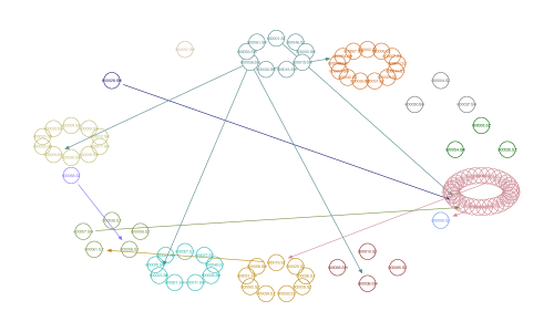
Figure 5.1: Visualization of the network structure given by the known $w$ observed in 2019, where the nodes represent the companies and the edges with direction indicate the links of cross ownership. The companies are clustered with different colors by sector classification.

It might be possible that $w_{j,k}=0$ while $h_{j,k}\neq 0$, if some shareholders of company $j$ are not revealed publicly. We set $w_{j,j}=h_{j,j}=0$. Without loss of generality, we assume that the misspecification error only occurs if the actual link is nonzero, i.e., the case that $w_{j,k}\neq 0$ while $h_{j,k}=0$ is ruled out. We aim at estimating the network effect $\rho$ and the misspecification errors $\delta_{j,k}=h_{j,k}-w_{j,k}$ by GDS using our proposed approach. In the end, we would like to recover the latent linkages $h_{j,k}$ based on the inference results on the deviations $h_{j,k}-w_{j,k}$.

In particular, the two-step DRGMM estimation procedure described in Section 2.3 is implemented, where the lags $r_{t-1},r_{t-2}$ are chosen as the IVs. We get $\hat{\rho}=0.2244$ and $\hat{\gamma}=0.0017$. To further justify the prediction performance of our proposed method, we define the prediction error by the root-mean-square deviation: $\sqrt{\sum_{j=1}^{p}\sum_{t=1}^{n}(\hat{r}_{j,t}-r_{j,t})^{2}}$, where the predicted returns are given by $\hat{r}_{j,t}=\hat{\rho}w_{j}^{\top}r_{t}+\hat{\rho}\hat{\delta}_{j}^{\top}r_{t}+\hat{\gamma}X_{j,t}$. In particular, we compare the prediction errors with two alternatives: spatial autoregressive (SAR) model solely based on the observed network structure $w$, and one-step GDS without debiasing. We consider the same moment conditions (i.e., same IVs) for all these competitors. We find that taking the possible misspecification into account and estimating the error via regularization would improve the cross-sectional prediction accuracy in the spatial network of stock returns by 3%. The two regularized approaches give comparable prediction performance.

Furthermore, it is of interest to carry out testing on the latent network structure, and the inference theory based on DRGMM enables us to do that formally. Following the discussion in Section 3.2, we perform individual inference on $H_{0}^{(j,k)}:\delta_{j,k}=0$ if $w_{j,k}$ is observed to be zero. The recovered network structure after hypothesis testings is shown in Figure 5.2, where a link from $k$ to $j$ indicates $\delta_{j,k}$ is significantly nonzero, i.e., $h_{j,k}$ is nonzero. We discover that the network accounting for latent link structure is sufficiently different from the pre-specified one. The results demonstrate the necessity of accounting for misidentification of the network links when analyzing the risk channels and financial stability within a financial system.

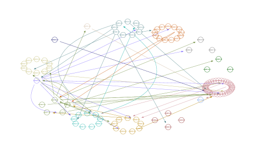
Figure 5.2: Visualization of the recovered network structure by DRGMM and individual testing using the data sample observed in 2019.

Appendix

Appendix A Detailed Proofs

A.1 Some Useful Lemmas

LEMMA A.1 (Weyls’ inequality for singular values).

Let $H$ ($m\times n$) be the exact matrix and $P$($m\times n$) be a perturbation matrix that represents the uncertainty. Consider the matrix $M=H+P$. If any two of $M$, $H$ and $P$ are $m$ by $n$ real matrices, where $M$ has singular values

$$\mu_{1}\geq\cdots\geq\mu_{\min{(m,n)}},$$

$H$ has singular values

$$\nu_{1}\geq\cdots\geq\nu_{\min{(m,n)}},$$

and $P$ has singular values

$$\rho_{1}\geq\cdots\geq\rho_{\min{(m,n)}}.$$

Then the following inequalities hold for $i=1,\ldots,\min(m,n)$, $1\leq k\leq\min(m,n)$,

$$\max_{0\leq i\leq\min(m,n)-k}\{\nu_{k+i}-\rho_{i+1},-\nu_{i+1}+\rho_{i+k},0\}\leq\mu_{k}\leq\min_{1\leq i\leq k}(\nu_{i}+\rho_{k-i+1}).$$

Proof.

The results is a direct consequence of Theorem 2 of Queiró and Sá, (1995) with completion of the $m\times n$ matrix to square matrix by letting the zero entries and the nonzero singular values stay the same. ∎

LEMMA A.2 (Corollary 3.3 of Lu and Pearce, (2000)).

Suppose that $B$ and $A$ are $m\times l$ and $l\times n$ matrices respectively, and let $p=\max\{m,n,l\}$ and $q=\min\{m,n,l\}$. Then for each $k=1,\cdots q$,

$$\sigma_{k}(BA)\leq\min_{1\leq i\leq k}\sigma_{i}(B)\sigma_{k+1-i}(A).$$

If $p<2q$, then for each $k=1,\ldots,2q-p$,

$$\max_{k+p-q\leq i\leq q}\sigma_{i}(B)\sigma_{p+k-i}(A)\leq\sigma_{k}(BA).$$

LEMMA A.3 (Theorem 6.2 of Zhang and Wu, (2017) Tail probabilities for high dimensional partial sums).

For a mean zero $p$-dimensional random variable $X_{t}\in R^{p}$ ($p>1$), let $S_{n}=\sum^{n}_{t=1}X_{t}$ and assume that $\||X_{\cdot}|_{\infty}\|_{q,\varsigma}<\infty,$ where $q>2$ and $\varsigma\geq 0$, and $\Phi_{2,\varsigma}=\max_{1\leq j\leq p}\|X_{j,\cdot}\|_{2,\varsigma}<\infty$. i) If $\varsigma>1/2-1/q$, then for $x\gtrsim\sqrt{n\log p}\Phi_{2,\varsigma}+n^{1/q}(\log p)^{3/2}\||X_{\cdot}|_{\infty}\|_{q,\varsigma}$,

$$\mathrm{P}(|S_{n}|_{\infty}\geq x)\leq\frac{C_{q,\varsigma}n(\log p)^{q/2}\||X_{\cdot}|_{\infty}\|^{q}_{q,\varsigma}}{x^{q}}+C_{q,\varsigma}\operatorname{exp}\bigg{(}\frac{-C_{q,\varsigma}x^{2}}{n\Phi^{2}_{2,\varsigma}}\bigg{)}.$$

ii) If $0<\varsigma<1/2-1/q$, then for $x\gtrsim\sqrt{n\log p}\Phi_{2,\varsigma}+n^{1/2-\varsigma}(\log p)^{3/2}\||X_{\cdot}|_{\infty}\|_{q,\varsigma}$,

$$\mathrm{P}(|S_{n}|_{\infty}\geq x)\leq\frac{C_{q,\varsigma}n^{q/2-\varsigma q}(\log p)^{q/2}\||X_{\cdot}|_{\infty}\|^{q}_{q,\varsigma}}{x^{q}}+C_{q,\varsigma}\operatorname{exp}\bigg{(}\frac{-C_{q,\varsigma}x^{2}}{n\Phi^{2}_{2,\varsigma}}\bigg{)}.$$

LEMMA A.4 (Tail probabilities for high dimensional partial sums with strong tail assumptions).

For a mean zero $p$-dimensional random variable $X_{t}\in R^{p}$ ($p>1$), let $S_{n}=\sum^{n}_{t=1}X_{t}$ and assume that $\Phi_{\psi_{\nu},\varsigma}=\max_{1\leq j\leq p}\sup_{q\geq 2}q^{-\nu}\|X_{j,\cdot}\|_{q,\varsigma}<\infty$ for some $\nu\geq 0$, and let $\gamma=2/(1+2\nu)$. Then for all $x>0$, we have

$$\mathrm{P}(|S_{n}|_{\infty}\geq x)\lesssim p\operatorname{exp}\{-C_{\gamma}x^{\gamma}/(\sqrt{n}\Phi_{\psi_{\nu},0})^{\gamma}\},$$

where $C_{\gamma}$ is a constant only depends on $\gamma$.

Lemma A.4 follows from Theorem 3 of Wu and Wu, (2016) and applying the Bonferroni inequality. In particular, $\nu=1$ corresponds to the sub-exponential case, and $\nu=1/2$ corresponds to the sub-Gaussian case.

LEMMA A.5 (Freedman’s inequality).

Let $\{\xi_{a,t}\}_{t=1}^{n}$ be a martingale difference sequence with respect to the filtration $\{\mathcal{F}_{t}\}_{t=1}^{n}$. Let $V_{a}=\sum^{n}_{t=1}\mathop{\mbox{\sf E}}(\xi^{2}_{a,t}|\mathcal{F}_{t-1})$ and $M_{a}=\sum^{n}_{t=1}\xi_{a,t}$. Then, for $x,u,v>0$, we have

$$\mathrm{P}(\max_{a\in\mathcal{A}}|M_{a}|\geq x)\leq\sum^{n}_{t=1}\mathrm{P}(\max_{a\in\mathcal{A}}\xi_{a,t}\geq u)+2\mathrm{P}(\max_{a\in\mathcal{A}}V_{a}\geq v)+2|\mathcal{A}|e^{-x^{2}/(2xu+2v)},$$

where $\mathcal{A}$ is an index set with $|\mathcal{A}|<\infty$.

Lemma A.5 is a maximal form of Freedman’s inequality (Freedman, , 1975).

LEMMA A.6 (Maximal inequality based on Freedman’s inequality).

Let $\{\xi_{a,t}\}_{t=1}^{n}$ be a martingale difference sequence with respect to the filtration $\{\mathcal{F}_{t}\}_{t=1}^{n}$, where $a\in\mathcal{A}$, $\mathcal{A}$ is an index set with $|\mathcal{A}|<\infty$. Suppose there exists $a^{\ast}\in\mathcal{A}$ such that $\max\limits_{a\in\mathcal{A}}|\sum_{t=1}^{n}\xi_{a,t}|\leq\sum_{t=1}^{n}|\xi_{a^{\ast},t}|$ and $\max\limits_{1\leq t\leq n}|\xi_{a^{\ast},t}|\leq F$, with $\|F\|_{2}$ is bounded. Let $V_{a}=\sum^{n}_{t=1}\mathop{\mbox{\sf E}}(\xi^{2}_{a,t}|\mathcal{F}_{t-1})$ and $M_{a}=\sum^{n}_{t=1}\xi_{a,t}$. Define the event $\mathcal{G}\stackrel{{\scriptstyle\mathrm{def}}}{{=}}\Big{\{}\max\limits_{a\in\mathcal{A},1\leq t\leq n}\xi_{a,t}\leq A,\max\limits_{a\in\mathcal{A}}V_{a}\leq B\Big{\}}$, where $A,B$ are constants. Given $\sqrt{n}\mathrm{P}(\mathcal{G}^{c})\lesssim A\log(1+|\mathcal{A}|)+\sqrt{B}\sqrt{\log(1+|\mathcal{A}|)}$, we have

$$\mathop{\mbox{\sf E}}\Big{[}\max_{a\in\mathcal{A}}|M_{a}|\Big{]}\lesssim A\log(1+|\mathcal{A}|)+\sqrt{B}\sqrt{\log(1+|\mathcal{A}|)}.$$

Proof.

Observe that

$$\mathop{\mbox{\sf E}}\Big{[}\max_{a\in\mathcal{A}}|M_{a}|\Big{]}=\mathop{\mbox{\sf E}}\Big{[}\max_{a\in\mathcal{A}}|M_{a}|\bm{1}(\mathcal{G})\Big{]}+\mathop{\mbox{\sf E}}\Big{[}\max_{a\in\mathcal{A}}|M_{a}|\bm{1}(\mathcal{G}^{c})\Big{]}.$$

The bound of the first part follows from a trivial modification of Lemma 19.33 in van der Vaart, (2000) based on Lemma A.5. The second part is bounded by Cauchy-Schwarz inequality and Burkholder inequality (Burkholder, , 1988)

$$\mathop{\mbox{\sf E}}\Big{[}\max_{a\in\mathcal{A}}|M_{a}|\bm{1}(\mathcal{G}^{c})\Big{]}\leq\sqrt{n}\{\mathop{\mbox{\sf E}}(F^{2})\}^{1/2}\{\mathrm{P}(\mathcal{G}^{c})\}^{1/2}.$$

Then the result follows from the assumption $\sqrt{n}\mathrm{P}(\mathcal{G}^{c})\lesssim A\log(1+|\mathcal{A}|)+\sqrt{B}\sqrt{\log(1+|\mathcal{A}|)}$.

∎

LEMMA A.7.

Consider a $p\times p$ positive semi-definite random matrix $H_{1}$ and a $p\times p$ deterministic positive definite matrix $H_{2}$. Assume that $|H_{1}-H_{2}|_{2}=\mathcal{O}_{\mathrm{P}}(c_{n})$, $c_{n}\to 0$. Then, we have

$$\lambda_{\min}(H_{1})=\lambda_{\min}(H_{2})-\mathcal{O}_{\mathrm{P}}(c_{n}).$$

Proof.

The results are implied by

$$\lambda_{\min}(H_{1})=\min_{v\in\mathbb{R}^{p},|v|_{2}=1}v^{\top}H_{1}v \geq\min_{v\in\mathbb{R}^{p},|v|_{2}=1}v^{\top}H_{2}v-\max_{v\in\mathbb{R}^{p},|v|_{2}=1}v^{\top}(H_{1}-H_{2})v$$

$$=\min_{v\in\mathbb{R}^{p},|v|_{2}=1}v^{\top}H_{2}v-|H_{1}-H_{2}|_{2}$$

$$\geq\lambda_{\min}(H_{2})-\mathcal{O}_{\mathrm{P}}(c_{n}).$$

∎

A.2 Identification for the Simple Model

As discussed in Section 2.1, we shall estimate $\beta^{0}$ in (2) by regularization. For instance, given $|\beta^{0}|_{0}=\mbox{\tiny$\mathcal{O}$}(n)$, a Dantzig selector estimator is defined as the solution to the following program:

$$\min_{\beta}|\beta|_{1}\quad\text{subject to}\quad|B^{\top}X^{\top}(y-XB\beta)|_{\infty}\leq\lambda,$$ (A.1)

where $\lambda>0$ is the tuning parameter.

Now the question is what condition we need to impose on $X$ such that a restricted isometry property (RIP) or restricted eigenvalue (RE) condition is ensured on the design matrix $XB$. Also, it may be helpful to understand the format of $B$ as well. For example, when $p=4$, $B^{\top}$ can take the form $\begin{pmatrix}1/4&1/4&1/4&1/4\\ 1&0&0&0\\ 0&1&0&0\\ 0&0&1&0\\ 0&0&0&1\end{pmatrix}$.

REMARK A.1 (Restriction on $B$ (for fixed design)).

We notice that for the full rank matrix $X$, if there exists a full rank matrix $A_{p\times(p-n)}$ ($\mathop{\rm{rank}}(A)=p-n$), such that $XA=0$ (i.e., the columns of $A$ form the null space of $X$), then for each $\xi\neq\xi^{0}$ ($\xi,\xi_{0}\in\mathbb{R}^{p}$), we can find a nonzero vector $\eta\in\mathbb{R}^{p-n}$ such that $\xi=A\eta+\xi_{0}$, if we have $X\xi=X\xi_{0}$. Thus, we shall restrict the columns of $B$ such that they do not belong to the space spanned by the columns of $A$, namely there does not exist a column of $B$, $B_{i}$, such that $B_{i}=A\eta$.

The RIP for $XB$ in the case that $X$ is deterministic is discussed in the following lemma.

LEMMA A.8.

Let $B_{I}$ denote the sub-matrix of $B$ with columns indexed by the set $I$ and the cardinality $|I|$ given by $s$ ($s\leq n$). Let $\mathcal{V}_{B_{I}}\stackrel{{\scriptstyle\mathrm{def}}}{{=}}\{\delta\in\mathbb{R}^{p}:\xi=B_{I}\xi_{I},\xi_{I}\in\mathcal{S}^{s-1}\}$, where $\mathcal{S}^{s-1}$ denotes the unit Euclidean sphere, i.e., $\xi_{I}$ is a unit vector with $|\xi_{I}|_{2}=1$. If $B_{I}$ is of rank $s$ for any $I$, and $c\leq\tilde{\lambda}_{s,B}\leq\lambda_{1}(X^{\top}X)\leq C$, $\tilde{\lambda}_{s,B}\stackrel{{\scriptstyle\mathrm{def}}}{{=}}\underset{I:|I|=s}{\min}\,\underset{\xi\in\mathcal{V}_{B_{I}}}{\min}\frac{\xi^{\top}X^{\top}X\xi}{\xi^{\top}\xi}$, then we have the RIP for $XB$.

Proof of Lemma A.8.

Note that to prove the RIP of $XB$ is equivalent to show that $c^{\prime}\leq\sigma_{s}(XB_{I})\leq\sigma_{1}(XB_{I})\leq C^{\prime}$.

Let $\mathcal{V}:\dim(\mathcal{V})=i$ be a subspace of $\mathbb{R}^{s}$ of dimension $i$, $i=1,\ldots,s$. Due to the Min-max theorem for singular values, we have

$$\lambda_{s}(B_{I}^{\top}X^{\top}XB_{I})=\sigma^{2}_{s}(XB_{I}) =\max\limits_{\mathcal{V}:\dim(\mathcal{V})=s}\,\min\limits_{\begin{subarray}{c}\xi_{I}\in\mathcal{V},\\ \xi_{I}^{\top}\xi_{I}=1\end{subarray}}\,\xi_{I}^{\top}B_{I}^{\top}X^{\top}XB_{I}\xi_{I}$$

$$=\min\limits_{\mathcal{V}:\dim(\mathcal{V})=1}\,\max\limits_{\begin{subarray}{c}\xi_{I}\in\mathcal{V},\\ \xi_{I}^{\top}\xi_{I}=1\end{subarray}}\,\xi_{I}^{\top}B_{I}^{\top}X^{\top}XB_{I}\xi_{I}.$$

For any fixed $\mathcal{V}:\dim(\mathcal{V})=s$, we have

$$\min\limits_{\begin{subarray}{c}\xi_{I}\in\mathcal{V},\\ \xi_{I}^{\top}\xi_{I}=1\end{subarray}}\frac{\xi_{I}^{\top}B_{I}^{\top}X^{\top}XB_{I}\xi_{I}}{\xi_{I}^{\top}\xi_{I}}$$

$$= \min\limits_{\begin{subarray}{c}\xi_{I}\in\mathcal{V},\\ \xi_{I}^{\top}\xi_{I}=1\end{subarray}}\frac{\xi_{I}^{\top}B_{I}^{\top}X^{\top}XB_{I}\xi_{I}}{\xi_{I}^{\top}B_{I}^{\top}B_{I}\xi_{I}}\frac{\xi_{I}^{\top}B_{I}^{\top}B_{I}\xi_{I}}{\xi_{I}^{\top}\xi_{I}}$$

$$\geq \min_{\xi\in\mathcal{V}_{B_{I}}}\frac{\xi^{\top}X^{\top}X\xi}{\xi^{\top}\xi}\lambda_{s}(B_{I}^{\top}B_{I})$$

$$\geq \tilde{\lambda}_{s,B}\lambda_{s}(B_{I}^{\top}B_{I}),$$

where the last inequality is due to the definition of $\tilde{\lambda}_{s,B}$ and the full rank property of $B_{I}^{\top}B_{I}$, which implies $\lambda_{\min}(B_{I}^{\top}B_{I})=\lambda_{s}(B_{I}^{\top}B_{I})$ is positive. As the above inequality holds for any subspace $\mathcal{V}$ of dimension $s$, thus we have $\lambda_{s}(B_{I}^{\top}X^{\top}XB_{I})\geq\tilde{\lambda}_{s,B}\lambda_{s}(B_{I}^{\top}B_{I})$. Similarly, we have $\lambda_{1}(B_{I}^{\top}X^{\top}XB_{I})\leq\lambda_{1}(X^{\top}X)\lambda_{1}(B_{I}^{\top}B_{I})$.

Given $\lambda_{s}(B_{I}^{\top}X^{\top}XB_{I})=\sigma_{s}^{2}(XB_{I})$, we have proved that if $B_{I}$ is of rank $s$ for any $I$, and $c\leq\tilde{\lambda}_{s,B}\leq\lambda_{1}(X^{\top}X)\leq C$, then the RIP for $XB$ follows. ∎

Next, we provide another Lemma for the random design $X$ with i.i.d. sub-Gaussian entries. We define $\|Z\|_{\psi_{1}}=\inf\{t<0:\mathop{\mbox{\sf E}}\operatorname{exp}(|Z|/t)\leq 2\}$ and $\|Z\|_{\psi_{2}}=\inf\{t<0:\mathop{\mbox{\sf E}}\operatorname{exp}(|Z|^{2}/t^{2})\leq 2\}$ as the sub-exponential norm and sub-Gaussian norm of the random variable $Z$.

LEMMA A.9.

Let $X$ be an $n\times p$ matrix whose rows $X_{i}$ are independent mean-zero sub-Gaussian isotropic random vectors in $\mathbb{R}^{p}$. Suppose $c\leq\sigma_{s}(B_{I})\leq\sigma_{1}(B_{I})\leq C$ and $n\gg s\log(pe/s)$. Then we have

$$c_{K}\sqrt{n}\leq\sigma_{s}(X^{\top}B_{I})\leq\sigma_{1}(X^{\top}B_{I})\leq C_{K}\sqrt{n},$$

with probability approaching one, where $c_{K},C_{K}$ are positive constants related to $K=\max_{i}\|X_{i}\|_{\psi_{2}}$.

Proof of Lemma A.9.

Step 1: For $\xi\in\mathcal{S}^{s-1}$, where $\mathcal{S}^{s-1}$ denotes the unit Euclidean sphere, i.e. $|\xi|_{2}=1$, we first show that $\xi^{\top}B_{I}^{\top}X_{i}X_{i}^{\top}B_{I}\xi$ is concentrated around its mean $\xi^{\top}B_{I}^{\top}B_{I}\xi$. Let $U_{i}\stackrel{{\scriptstyle\mathrm{def}}}{{=}}\xi^{\top}B_{I}^{\top}X_{i}X_{i}^{\top}B_{I}\xi-\xi^{\top}B_{i}^{\top}B_{i}\xi$. By Bernstein inequality, we have

$$\mathrm{P}\Big{(}\Big{|}n^{-1}\sum_{t=1}^{n}U_{i}\Big{|}\geq{\varepsilon}/2\Big{)} \leq 2\,\operatorname{exp}\Big{(}-c\min\Big{(}\frac{{\varepsilon}^{2}n^{2}}{\sum_{t=1}^{n}\|U_{i}\|_{\psi_{1}}^{2}},\frac{{\varepsilon}n}{\max\limits_{1\leq i\leq n}\|U_{i}\|_{\psi_{1}}}\Big{)}\Big{)}.$$

By utilizing the properties of sub-Gaussian and sub-exponential random variables, we have

$$\|U_{i}\|_{\psi_{1}}\leq C_{1}\|(\xi^{\top}B_{I}^{\top}X_{i})^{2}\|_{\psi_{1}} = C_{1}\|\xi^{\top}B_{I}^{\top}X_{i}\|_{\psi_{2}}^{2}$$

$$\leq C_{1}\Big{\|}\sum_{j=1}^{s}\xi_{j}B_{I,j}^{\top}X_{i}\Big{\|}^{2}_{\psi_{2}}$$

$$\leq C_{1}\sum_{j=1}^{s}\xi_{j}^{2}\|B_{I,j}^{\top}X_{i}\|^{2}_{\psi_{2}}$$

$$\leq C_{1}\max_{1\leq j\leq s}\|B_{I,j}^{\top}X_{i}\|_{\psi_{2}}^{2}\leq C_{2}\lambda_{\max}(B_{I}^{\top}B_{I})=:K,$$

where $B_{I,j},j=1,\ldots,s$ is the $j$-th column vector of $B_{I}$ and the last inequality follows given $\max\limits_{1\leq j\leq s}\|B_{I,j}^{\top}X_{i}\|^{2}_{\psi_{2}}\leq\max\limits_{1\leq j\leq s}|B_{I,j}|_{2}^{2}\max\limits_{1\leq k\leq p}\|X_{i,k}\|_{\psi_{2}}^{2}\leq C\lambda_{\max}(B_{I}^{\top}B_{I})$. It follows that

$$\mathrm{P}\Big{(}\Big{|}n^{-1}\sum_{t=1}^{n}U_{i}\Big{|}\geq{\varepsilon}/2\Big{)} \leq 2\,\operatorname{exp}\Big{(}-c\min\Big{(}\frac{{\varepsilon}^{2}}{K^{2}},\frac{{\varepsilon}}{K}n\Big{)}\Big{)}.$$

Step 2: Let $\overline{\sigma}\stackrel{{\scriptstyle\mathrm{def}}}{{=}}\sigma_{1}(B_{I})$, and $\underline{\sigma}=\sigma_{s}(B_{I})$, which are bounded positive constants.

Note that

$$|n^{-1}B_{I}^{\top}X^{\top}XB_{I}-B_{I}^{\top}B_{I}|_{2}=\sup_{\xi\in\mathcal{S}^{s-1}}|{n}^{-1}\xi^{\top}B_{I}^{\top}X^{\top}XB_{I}\xi-\xi^{\top}B_{I}^{\top}B_{I}\xi|.$$

Moreover, for any $\xi\in\mathcal{S}^{s-1}$, we have

$$\big{|}n^{-1}|\xi^{\top}B_{I}^{\top}X^{\top}|_{2}^{2}-|\xi^{\top}B_{I}^{\top}|_{2}^{2}\big{|}$$

$$= \big{|}1/\sqrt{n}|\xi^{\top}B_{I}^{\top}X^{\top}|_{2}-|\xi^{\top}B_{I}|_{2}\big{|}\big{(}1/\sqrt{n}|\xi^{\top}B_{I}^{\top}X^{\top}|_{2}+|\xi^{\top}B_{I}|_{2}\big{)}$$

$$\geq |\xi^{\top}B_{I}^{\top}|_{2}\big{|}1/\sqrt{n}|\xi^{\top}B_{I}^{\top}X^{\top}|_{2}-|\xi^{\top}B_{I}^{\top}|_{2}|\big{|}\geq\underline{\sigma}\big{|}1/\sqrt{n}|\xi^{\top}B_{I}^{\top}X^{\top}|_{2}-|\xi^{\top}B_{I}^{\top}|_{2}|\big{|}.$$

Therefore, we have shown that $|n^{-1}B_{I}^{\top}X^{\top}XB_{I}-B_{I}^{\top}B_{I}|_{2}\leq{\varepsilon}$ holds with high probability implies ${\varepsilon}{\sqrt{n}}(\underline{\sigma}-{\varepsilon}/\underline{\sigma})\leq\sigma_{s}(XB_{I})\leq\sigma_{1}(XB_{I})\leq{\varepsilon}{\sqrt{n}}(\overline{\sigma}+{\varepsilon}/\underline{\sigma})$ holds with the same probability.

Step 3: By applying the Corollary 4.2.13 of Vershynin, (2019), we can find a $1/4$-net $\mathcal{N}$ of the unit sphere $\mathcal{S}^{s-1}$ with cardinality $|\mathcal{N}|\leq 9^{s}$. By the discretized property of the net, we have

$$|n^{-1}B_{I}^{\top}X^{\top}XB_{I}-B_{I}^{\top}B_{I}|_{2} = \sup_{\xi\in\mathcal{S}^{s-1}}|{n}^{-1}\xi^{\top}B_{I}^{\top}X^{\top}XB_{I}\xi-\xi^{\top}B_{I}^{\top}B_{I}\xi|$$

$$\leq 2\sup_{\xi\in\mathcal{N}}|{n}^{-1}\xi^{\top}B_{I}^{\top}X^{\top}XB_{I}\xi-\xi^{\top}B_{I}^{\top}B_{I}\xi|.$$

Using the union bounds, we obtain

$$\mathrm{P}\Big{(}\sup_{\xi\in\mathcal{N}}|{n}^{-1}\xi^{\top}B_{I}^{\top}X^{\top}XB_{I}\xi-\xi^{\top}B_{I}^{\top}B_{I}\xi|\geq{\varepsilon}/2\Big{)}\leq 2\cdot 9^{s}\operatorname{exp}\big{(}-c\min({\varepsilon}^{2}/K^{2},{\varepsilon}/K)n\big{)}.$$

We have proved that the pointwise concentration in Step 1 implies that $|n^{-1}B_{I}^{\top}X^{\top}XB_{I}-B_{I}^{\top}B_{I}|_{2}\leq{\varepsilon}$ holds with high probability.

Step 4: By Step 2 and 3 we know that provided $n\min({\varepsilon}^{2}/K^{2},{\varepsilon}/K)\gg s\log 9$ we can get

$${\varepsilon}{\sqrt{n}}(\underline{\sigma}-{\varepsilon}/\underline{\sigma})\leq\sigma_{s}(XB_{I})\leq\sigma_{1}(XB_{I})\leq{\varepsilon}{\sqrt{n}}(\overline{\sigma}+{\varepsilon}/\underline{\sigma})$$

holds with probability $2\operatorname{exp}\big{(}-c^{\prime}\min({\varepsilon}^{2}/K^{2},{\varepsilon}/K)n\big{)}$. In addition, we know that there are $p\choose s$ ($\leq(pe/s)^{s}$) set of $I$ among the $p$ dimensional covariates. Thus, by the union bounds, we can bound the probability by

$$1-2\operatorname{exp}\big{(}-c^{\prime}\min({\varepsilon}^{2}/K^{2},{\varepsilon}/K)n+s\log(pe/s)\big{)}.$$

∎

We have shown in a simple high-dimensional linear regression case that our framework goes through with a modified design matrix. The identification issues under the general model are discussed in Section 3.1.2.

A.3 Proofs of Section 3.1

Proof of Lemma 3.2.

Similarly to the proof of Lemma A.8, we observe that

$$\sigma^{2}_{\min}(\Sigma^{xz}_{H}B_{I}) =\lambda_{\min}(B_{I}^{\top}{\Sigma_{H}^{xz}}^{\top}\Sigma^{xz}_{H}B_{I})\geq\min_{\xi\in\mathcal{V}_{B_{I}}}\frac{\xi^{\top}{\Sigma_{H}^{xz}}^{\top}\Sigma^{xz}_{H}\xi}{\xi^{\top}\xi}\lambda_{\min}(B_{I}^{\top}B_{I}),$$

$$\sigma^{2}_{\max}(\Sigma^{xz}_{H}B_{I}) =\lambda_{\max}(B_{I}^{\top}{\Sigma_{H}^{xz}}^{\top}\Sigma^{xz}_{H}B_{I})\leq\lambda_{\max}(B_{I}^{\top}B_{I})\lambda_{\max}({\Sigma_{H}^{xz}}^{\top}\Sigma_{H}^{xz}).$$

Consequently, we have

$$\min_{|I|\leq m}\max_{|H|\leq m}\sigma^{2}_{\min}(\Sigma^{xz}_{H}B_{I}) \geq\sigma_{\min,B}(m,\Sigma^{xz}_{H})\min_{|I|\leq m}\lambda_{\min}(B_{I}^{\top}B_{I}),$$

$$\max_{|I|\leq m}\max_{|H|\leq m}\sigma^{2}_{\max}(\Sigma^{xz}_{H}B_{I}) \leq\max_{|I|\leq m}\lambda_{\max}(B_{I}^{\top}B_{I})\max_{|H|\leq m}\lambda_{\max}({\Sigma_{H}^{xz}}^{\top}\Sigma_{H}^{xz}).$$

It follows that for some constants $c^{\prime},C^{\prime}>0$, we have $\sigma_{\min}(m,G)>c^{\prime}$ and $\sigma_{\max}(m,G)<C^{\prime}$. ∎

Proof of Lemma 3.3.

The proof follows that of Corollary 2 of Belloni et al., (2017) with the concentration inequality therein replaced by applying Lemma A.3 on the matrix $G$.

According to the triangle inequality, we have

$$|\hat{G}\theta|_{\infty}/|\theta|_{a}\geq-|(\hat{G}-G)\theta|_{\infty}/\|\theta\|_{a}+|G\theta|_{\infty}/\|\theta\|_{a}=:-T_{n,1}+T_{n,2}.$$

$T_{n,1}$ is handled by applying the concentration inequality in Lemma A.3. In particular, $|(\hat{G}-G)\theta|_{\infty}/|\theta|_{a}\leq|\hat{G}-G|_{\max}|\theta|_{1}/|\theta|_{a}$. Note that if $a=1$, $|\theta|_{1}/|\theta|_{a}=1$, and if $a=2$, $|\theta|_{1}/|\theta|_{a}\leq(1+u)s^{1/2}$. As we have shown in Section 3.1.1, $|\hat{G}-G|_{\max}\lesssim_{\mathrm{P}}b_{n}$, thus we have $-T_{n,1}\lesssim_{\mathrm{P}}b_{n}(1+u)s^{1-1/a}$.

The rest of the proof follows from Theorem 1 and Corollary 2 of Belloni et al., (2017). Provided $\sigma_{\min}(m,G)>c^{\prime}$ and $\sigma_{\max}(m,G)<C^{\prime}$, we can obtain the conclusion that $\kappa^{\hat{G}}_{a}(s,u)\geq s^{-1/a}C(u)$ with $a\in\{1,2\}$, given $b_{n}(1+u)s\lesssim C(u)$ holds for sufficiently large $n$ and $C(u)=\tilde{c}/(1+u)^{2}$. ∎

Proof of Theorem 3.1.

Lemma 3.3 implies that (A2) is satisfied with $\rho(\epsilon_{n}+\lambda_{n},\theta^{0},a)\asymp(\epsilon_{n}+\lambda_{n})\kappa_{a}^{\hat{G}}(s,u)^{-1}\lesssim(\epsilon_{n}+\lambda_{n})s^{1/a}C(u)^{-1}$. Combining the results in Lemma 3.1 leads to the conclusions. ∎

A.4 Convergence Rates of the Approximate Inverse Matrices

Define the class of matrices

$$\mathcal{U}\stackrel{{\scriptstyle\mathrm{def}}}{{=}}\mathcal{U}(b,s_{0}(q))=\Big{\{}\Upsilon:\Upsilon\succ 0,|\Upsilon|_{1}\leq M,\max_{1\leq i\leq q}\sum^{q}_{j=1}|\Upsilon_{ij}|^{b}\leq s_{0}(q)\Big{\}}$$

for $0\leq b<1$, where $\Upsilon=(\Upsilon_{ij})$ and the notation $\Upsilon\succ 0$ indicates that $\Upsilon$ is positive definite.

LEMMA A.10.

Assume that $\Upsilon^{0}=\Omega^{-1}\in\mathcal{U}(b,s_{0}(q))$. Select $\ell^{\Upsilon}_{n}$ such that $|\hat{\Omega}-\Omega|_{\max}M\leq\ell_{n}^{\Upsilon}$ with probability approaching $1$ (the detailed rate of $\ell^{\Upsilon}_{n}$ is specified in Lemma A.13). Then, we have

$$|\hat{\Upsilon}-\Upsilon^{0}|_{\max}\leq 4M\ell^{\Upsilon}_{n}=:\rho_{n}^{\Upsilon}$$

holds with probability approaching $1$, Moreover, with probability approaching $1$, we have

$$|\hat{\Upsilon}-\Upsilon^{0}|_{2}\leq C_{b}(4M\ell^{\Upsilon}_{n})^{1-r}s_{0}(q)=:\rho_{n,2}^{\Upsilon},$$

where $C_{b}$ is a positive constant only depends on $b$.

Proof.

Recall that $\hat{\Upsilon}^{1}$ is the solution of (7). We first observe that

$$|\hat{\Upsilon}^{1}-\Upsilon^{0}|_{\max} \leq |\Upsilon^{0}\Omega(\hat{\Upsilon}^{1}-\Upsilon^{0})|_{\max}$$

$$\leq |\Omega(\hat{\Upsilon}^{1}-\Upsilon^{0})|_{\max}|\Upsilon^{0}|_{1}$$

$$|\Omega(\hat{\Upsilon}^{1}-\Upsilon^{0})|_{\max} \leq |(\Omega-\hat{\Omega})(\hat{\Upsilon}^{1}-\Upsilon^{0})|_{\max}+|\hat{\Omega}(\hat{\Upsilon}^{1}-\Upsilon^{0})|_{\max}=:R_{n,1}+R_{n,2}.$$

In particular, we have $R_{n,1}\leq 2|\Omega-\hat{\Omega}|_{\max}M\leq 2\ell^{\Upsilon}_{n}$ holds with probability tending $1$, and $R_{n,2}\leq|\hat{\Omega}\Upsilon^{0}-\mathbf{I}_{q}|_{\max}+|\hat{\Omega}\hat{\Upsilon}^{1}-\mathbf{I}_{q}|_{\max}\lesssim_{\mathrm{P}}2\ell_{n}^{\Upsilon}$. According to the definition given by (8), it follows that $|\hat{\Upsilon}-\Upsilon^{0}|_{\max}\leq 4M\ell^{\Upsilon}_{n}$ with probability approaching $1$. The rate of $\ell^{\Upsilon}_{n}$ will depend on the concentration inequalities we use.

Moreover, with probability approaching $1$, we have

$$|\hat{\Upsilon}-\Upsilon^{0}|_{2}\leq\sqrt{|\hat{\Upsilon}-\Upsilon^{0}|_{1}|\hat{\Upsilon}-\Upsilon^{0}|_{\infty}}=|\hat{\Upsilon}-\Upsilon^{0}|_{1}\leq C_{b}(4M\ell^{\Upsilon}_{n})^{1-b}s_{0}(q),$$

where $C_{b}$ is a positive constant only depends on $b$. The rate of $|\hat{\Upsilon}-\Upsilon^{0}|_{1}$ follows from the proof of Theorem 6 in Cai et al., (2011). ∎

Similarly, we define the class of matrices

$$\widetilde{\mathcal{U}}\stackrel{{\scriptstyle\mathrm{def}}}{{=}}\widetilde{\mathcal{U}}(b,s_{0}(K^{(1)}))=\Big{\{}\Pi:\Pi\succ 0,|\Pi|_{1}\leq M,\max_{1\leq i\leq K^{(1)}}\sum^{K^{(1)}}_{j=1}|\Pi_{ij}|^{b}\leq s_{0}(K^{(1)})\Big{\}}$$

for $0\leq b<1$, where $\Pi=(\Pi_{ij})$. The lemma below follows.

LEMMA A.11.

Assume that $\Pi^{0}=(G_{1}^{\top}\Upsilon^{0}G_{1})^{-1}\in\widetilde{\mathcal{U}}(b,s_{0}(K^{(1)}))$. Select $\ell_{n}^{\Pi}$ such that $|G_{1}^{\top}\Upsilon^{0}G_{1}-\hat{G}_{1}^{\top}\hat{\Upsilon}\hat{G}_{1}|_{\max}M\leq\ell_{n}^{\Pi}$ with probability approaching $1$ (see Lemma A.15 for the specific rate of $\ell_{n}^{\Pi}$). Then, we have

$$|\hat{\Pi}-\Pi^{0}|_{\max}\leq 4M\ell_{n}^{\Pi}=:\rho_{n}^{\Pi}$$

and

$$|\hat{\Pi}-\Pi^{0}|_{2}\leq C_{b}(4M\ell_{n}^{\Pi})^{1-b}s_{0}(K^{(1)})=:\rho_{n,2}^{\Pi}$$

hold with probability approaching $1$, respectively.

Proof.

The proof is similar to that of Lemma A.10 and thus is omitted. ∎

Recall that $D\stackrel{{\scriptstyle\mathrm{def}}}{{=}}G_{1}^{\top}\Upsilon^{0}G_{1}=(\Pi^{0})^{-1}$ and $F\stackrel{{\scriptstyle\mathrm{def}}}{{=}}G_{1}^{\top}\Upsilon^{0}G_{2}\Xi^{0}G_{2}^{\top}\Upsilon^{0}G_{1}$. Next, we show the rate of the estimator of $B=({D}+{F})^{-1}=((\Pi^{0})^{-1}+F)^{-1}$ given by $\hat{B}=\hat{\Pi}-\hat{\Pi}(\mathbf{I}_{q}+\hat{F}\hat{\Pi})^{-1}\hat{F}\hat{\Pi}$. Denote by $\rho_{n,2}^{F}$ the rate such that $|\hat{F}-F|_{2}\lesssim_{\mathrm{P}}\rho_{n,2}^{F}$. We shall discuss the conditions on this rate in Lemma A.15.

LEMMA A.12.

Under the conditions of Lemma A.11, suppose that there exist constants $c_{1},c_{2},c_{3}$ such that $c_{1}\leq\sigma_{\min}(F\Pi^{0})\leq\sigma_{\max}(F\Pi^{0})\leq c_{2}$ and $\sigma_{\max}(F)\vee\sigma_{\max}(\Pi^{0})\leq c_{3}$. Assume that there exists a constant $C>0$ such that $|(\mathbf{I}-F\Pi^{0})^{-1}|_{2}\leq C$ and $|(\mathbf{I}-\hat{F}\hat{\Pi})^{-1}|_{2}\leq C$. Then, we have

$$|\hat{B}-B|_{\max}\lesssim_{\mathrm{P}}(\rho_{n}^{\Pi}\vee\rho_{n,2}^{\Pi}\vee\rho_{n,2}^{F})=:\rho_{n}^{B}.$$

Proof.

We first observe that

$$|\hat{B}-B|_{\max} \leq|\hat{\Pi}-\Pi^{0}|_{\max}+|(\hat{\Pi}-\Pi^{0})(\mathbf{I}-{F}\Pi^{0})^{-1}{F}\Pi^{0}|_{\max}$$

$$\quad+|\hat{\Pi}\{(\mathbf{I}-\hat{F}\hat{\Pi})^{-1}-(\mathbf{I}-{F}\Pi^{0})^{-1}\}{F}\Pi^{0}\}|_{\max}+|\hat{\Pi}(\mathbf{I}-\hat{F}\hat{\Pi})^{-1}(\hat{F}\hat{\Pi}-F\Pi^{0})|_{\max}$$

$$\lesssim_{\mathrm{P}}\rho_{n}^{\Pi}+|\hat{\Pi}-\Pi^{0}|_{2}|(\mathbf{I}-{F}\Pi^{0})^{-1}|_{2}|{F}\Pi^{0}|_{2}$$

$$\quad+|\hat{\Pi}|_{2}|(\mathbf{I}-\hat{F}\hat{\Pi})^{-1}-(\mathbf{I}-{F}\Pi^{0})^{-1}|_{2}|{F}\Pi^{0}|_{2}+|\hat{\Pi}|_{2}|(\mathbf{I}-\hat{F}\hat{\Pi})^{-1}|_{2}|\hat{F}\hat{\Pi}-F\Pi^{0}|_{2}.$$

By applying Lemma A.11, we obtain that

$$|\hat{\Pi}|_{2}\leq|\hat{\Pi}-\Pi^{0}|_{2}+|\Pi^{0}|_{2}\lesssim_{\mathrm{P}}\rho_{n,2}^{\Pi}+c_{3}$$

Besides, we have

$$|\hat{F}\hat{\Pi}-F\Pi^{0}|_{2}\leq|\hat{F}-F|_{2}|\hat{\Pi}|_{2}+|\hat{\Pi}-\Pi^{0}|_{2}|F|_{2}\lesssim_{\mathrm{P}}\rho_{n,2}^{F}c_{3}+\rho_{n,2}^{\Pi}c_{3}\lesssim\rho_{n,2}^{F}\vee\rho_{n,2}^{\Pi},$$

and

$$|(\mathbf{I}-\hat{F}\hat{\Pi})^{-1}-(\mathbf{I}-{F}\Pi^{0})^{-1}|_{2}\leq|(\mathbf{I}-F\Pi^{0})^{-1}|_{2}|(\mathbf{I}-\hat{F}\hat{\Pi})^{-1}|_{2}|\hat{F}\hat{\Pi}-F\Pi^{0}|_{2}\lesssim_{\mathrm{P}}\rho_{n,2}^{F}\vee\rho_{n,2}^{\Pi}.$$

Finally, the desired conclusion follows by collecting all the results above.

∎

In this Lemma we assume that $|(\mathbf{I}-F\Pi^{0})^{-1}|_{2}\leq C$, which can be implied by the condition $\sigma_{\min}(F\Pi^{0})>1$ or $\sigma_{\max}(F\Pi^{0})<1$. For example, given $1<c_{1}\leq\sigma_{\min}(F\Pi^{0})$, we have

$$|(\mathbf{I}-F\Pi^{0})^{-1}|_{2}\leq(\sigma_{\min}(\mathbf{I}-F\Pi^{0}))^{-1}\leq(\sigma_{\min}(F\Pi^{0})-1)^{-1}\leq(c_{1}-1)^{-1},\,c_{1}>1,$$

where the first inequality is implied by Lemma A.2, and the second one is due to Lemma A.1. Additionally, based on Lemma A.7, on the event $\{\sigma_{\min}(\hat{F}\hat{\Pi})>1\}$, which holds with probability approaching 1, it follows that

$$|(\mathbf{I}-\hat{F}\hat{\Pi})^{-1}|_{2} \leq(\sigma_{\min}(\mathbf{I}-\hat{F}\hat{\Pi}))^{-1}$$

$$\leq(\sigma_{\min}(\hat{F}\hat{\Pi})-1)^{-1}$$

$$\leq(\lambda_{\min}(\hat{F})\lambda_{\min}(\hat{\Pi})-1)^{-1}$$

$$\lesssim_{\mathrm{P}}\{(\lambda_{\min}(F)-\rho_{n,2}^{F})(\lambda_{\min}(\Pi^{0})-\rho_{n,2}^{\Pi})-1\}^{-1}\lesssim C.$$

REMARK A.2.

The rate of $|\hat{B}-B|_{\infty}$ shall follow similarly once we have dealt with the rate of $|\hat{V}-V|_{\infty}$, where $V\stackrel{{\scriptstyle\mathrm{def}}}{{=}}(\mathbf{I}-F\Pi^{0})^{-1}$ and $\hat{V}\stackrel{{\scriptstyle\mathrm{def}}}{{=}}(\mathbf{I}-\hat{F}\hat{\Pi})^{-1}$. In particular, provided $|\hat{V}-V|_{\max}\lesssim_{\mathrm{P}}\rho_{n}^{V}=\mbox{\tiny$\mathcal{O}$}(1)$, analogue to Lemma A.14, we have $|\hat{V}-V|_{\infty}\lesssim_{\mathrm{P}}\rho_{n,2}^{V}$, with $\rho_{n,2}^{V}=s(V)\rho_{n}^{V}$ if we assume $|V|_{0}=s(V)$ while $\rho_{n,2}^{V}=\nu(\rho_{n}^{V})^{1-l}$ in the case of $(|V|_{\infty,l}\vee|V|_{\infty})\leq\nu$ for some $0\leq l<1$. Finally, given $\max\{|\Pi^{0}|_{\infty},|F|_{\infty},|V|_{\infty}\}\leq\nu$, applying the results in Lemma A.11 shows that $|\hat{B}-B|_{\infty}\lesssim_{\mathrm{P}}\nu^{3}(\rho_{n,2}^{F}\vee\rho_{n,2}^{\Pi})=:\rho_{n,2}^{B}$, provided that $\rho_{n,2}^{\Pi},\rho_{n,2}^{V}\to 0$ as $n\to\infty$.

A.5 Proofs of Section 3.2 and Detailed Rate of $|r_{n}|_{\infty}$ for Linear Case

Proof of Theorem 3.2.

According to Lemma A.12 and A.15, we have $|\hat{A}\hat{G}_{1}-AG_{1}|_{\max}\lesssim_{\mathrm{P}}\ell_{n}^{\Pi}/M+\rho_{n,2}^{F}$ and $|\hat{B}-B|_{\max}\lesssim_{\mathrm{P}}\rho_{n}^{B}=\rho_{n}^{\Pi}\vee\rho_{n,2}^{\Pi}\vee\rho_{n,2}^{F}$. Based on the Gaussian approximation results as discussed in Section 3.2.2, we have $|\hat{g}(\theta^{0})|_{\infty}\lesssim_{\mathrm{P}}n^{-1/2}(\log q)^{1/2}$. On the event $\{|\hat{A}\hat{G}_{1}|_{1}\lesssim\omega_{1}^{3/2}\}$, which holds with probability approaching 1, applying the results in (10) as well as Remarks A.2 and A.8, we obtain

$$|r_{n,1}|_{\infty} \lesssim_{\mathrm{P}}\vartheta(\ell_{n}^{\Pi}/M+\rho_{n,2}^{F})d_{n,1}+\rho_{n}^{B}\omega_{1}d_{n,1}=:\varrho_{n,1},$$

$$|r_{n,3}|_{\infty} \lesssim_{\mathrm{P}}\{\rho_{n,2}^{B}\iota+(\vartheta+\rho_{n,2}^{B})\rho_{n,2}^{A}\}n^{-1/2}(\log q)^{1/2}=:\varrho_{n,3}.$$ (A.2)

We note that $r_{n,2}=0$ in linear moment models. ∎

We shall discuss the detailed rates of $\ell_{n}^{\Upsilon},\ell_{n}^{\Pi},\rho_{n,2}^{F}$ which are involved in the rate of $|r_{n}|_{\infty}$ in the following. And a concluding remark on the rate of $|r_{n}|_{\infty}$ is provided in Remark A.9.

Recall that in the case of linear moment models, the score functions are given by $g_{j}(D_{j,t},\theta)=z_{j,t}{\varepsilon}_{j}(D_{j,t},\theta)$, where ${\varepsilon}_{j}(D_{j,t},\theta)=y_{j,t}-\tilde{x}_{j,t}^{\top}\beta_{j}$. To simplify the notations, we shall denote $g_{jm,t}\stackrel{{\scriptstyle\mathrm{def}}}{{=}}z_{jm,t}{\varepsilon}_{j}(D_{j,t},\theta^{0})$ and $\hat{g}_{jm,t}\stackrel{{\scriptstyle\mathrm{def}}}{{=}}z_{jm,t}{\varepsilon}_{j}(D_{j,t},\hat{\theta})$, for all $j=1,\ldots,p$, and $m=1,\ldots,q_{j}$. We note that when the time series is non-stationary and the mean varies with respect to $t$, we can replace $\mathop{\mbox{\sf E}}(g_{il,t}g_{jm,t})$ by $\mathop{\mbox{\sf E}}_{n}\mathop{\mbox{\sf E}}(g_{il,t}g_{jm,t})$.

Let $C_{xz}$ and $C_{xz{\varepsilon}}$ be constants such that $\max_{i,j,l,m}|\mathop{\mbox{\sf E}}(\tilde{x}_{i,t}\tilde{x}_{j,t}^{\top}z_{il,t}z_{jm,t})|_{\max}\leq C_{xz}$ and $\max_{i,j,l,m}|\mathop{\mbox{\sf E}}(\tilde{x}_{i,t}z_{jm,t}z_{il,t}{\varepsilon}_{i,t}))|_{\infty}\leq C_{xz{\varepsilon}}$, respectively.

LEMMA A.13 (Rate of $\ell_{n}^{\Upsilon}$).

Under conditions in Lemma 3.1 and 3.3, we have

$$|\hat{\Omega}-{\Omega}|_{\max}\lesssim_{\mathrm{P}}\ell_{n}^{\Upsilon}/M,$$

given $d_{n,1}^{2}(C_{xz}+\gamma_{n})+d_{n,1}(C_{xz{\varepsilon}}+\gamma^{\prime}_{n})+\gamma_{n,1}+\gamma_{n,2}\lesssim\ell_{n}^{\Upsilon}/M$, where $d_{n,1}$ is defined in (10), $\gamma_{n},\gamma^{\prime}_{n},\gamma_{n,1},\gamma_{n,2}$ are specified in (A.3), (A.4) and (A.5).

Proof.

We first observe that

$$|\hat{\Omega}-{\Omega}|_{max} = \max_{i,j,l,m}|{\mathop{\mbox{\sf E}}}_{n}(\hat{g}_{il,t}\hat{g}_{jm,t})-\mathop{\mbox{\sf E}}(g_{il,t}g_{jm,t})|$$

$$\leq \max_{i,j,l,m}|{\mathop{\mbox{\sf E}}}_{n}\{(\hat{g}_{il,t}-g_{il,t})(\hat{g}_{jm,t}-g_{jm,t})\}|+2\max_{i,j,l,m}|{\mathop{\mbox{\sf E}}}_{n}\{g_{il,t}(\hat{g}_{jm,t}-g_{jm,t})\}|$$

$$+\max_{i,j,l,m}|{\mathop{\mbox{\sf E}}}_{n}(g_{il,t}g_{jm,t})-\mathop{\mbox{\sf E}}(g_{il,t}g_{jm,t})|$$

$$=: I_{n,1}+I_{n,2}+I_{n,3}$$

For $I_{n,1}$, it can be seen that

$$I_{n,1} \leq \max_{i,j,l,m}|\hat{\beta}_{i}-\beta_{i}^{0}|_{1}|\hat{\beta}_{j}-\beta_{j}^{0}|_{1}|{\mathop{\mbox{\sf E}}}_{n}(\tilde{x}_{i,t}\tilde{x}_{j,t}^{\top}z_{il,t}z_{jm,t})|_{\max}$$

$$\leq |\hat{\theta}-\theta^{0}|_{1}^{2}\{C_{xz}+|{\mathop{\mbox{\sf E}}}_{n}(\tilde{x}_{i,t}\tilde{x}_{j,t}^{\top}z_{il,t}z_{jm,t})-\mathop{\mbox{\sf E}}(\tilde{x}_{i,t}\tilde{x}_{j,t}^{\top}z_{il,t}z_{jm,t})|_{\max}\}.$$

Let $\chi_{t}^{ijlm}\stackrel{{\scriptstyle\mathrm{def}}}{{=}}\operatorname{vec}(\tilde{x}_{i,t}\tilde{x}_{j,t}^{\top}z_{il,t}z_{jm,t})=(\chi_{k,t}^{ijlm})_{k=1}^{K_{i}*K_{j}}$ and define

$$\gamma_{n}\stackrel{{\scriptstyle\mathrm{def}}}{{=}}cn^{-1/2}(\log P_{n})^{1/2}\max_{i,j,l,m,k}\|\chi_{k,\cdot}^{ijlm}\|_{2,\varsigma}+cn^{-1}c_{n,\varsigma}(\log P_{n})^{3/2}\|\max_{i,j,l,m}|\chi_{\cdot}|_{\infty}\|_{r,\varsigma},$$ (A.3)

with $P_{n}=(q\vee n\vee e)$, $c_{n,\varsigma}=n^{1/r}$ for $\varsigma>1/2-1/r$ and $c_{n,\varsigma}=n^{1/2-\varsigma}$ for $0<\varsigma<1/2-1/r$. By applying Lemma A.3 and the results in (10), we have $I_{n,1}\lesssim_{\mathrm{P}}d_{n,1}^{2}(C_{xz}+\gamma_{n})$, for sufficiently large $c$.

Similarly,

$$I_{n,2} \leq 2\max_{i,j,l,m}|\hat{\beta}_{j}-\beta_{j}^{0}|_{1}{\mathop{\mbox{\sf E}}}_{n}(\tilde{x}_{i,t}z_{jm,t}z_{il,t}{\varepsilon}_{i,t})|_{\infty}$$

$$\leq 2|\hat{\theta}-\theta^{0}|_{1}\{C_{xz{\varepsilon}}+|{\mathop{\mbox{\sf E}}}_{n}(\tilde{x}_{i,t}z_{jm,t}z_{il,t}{\varepsilon}_{i,t})-\mathop{\mbox{\sf E}}(\tilde{x}_{i,t}z_{jm,t}z_{il,t}{\varepsilon}_{i,t})|_{\infty}\}.$$

Let $\zeta_{t}^{ijlm}\stackrel{{\scriptstyle\mathrm{def}}}{{=}}\tilde{x}_{i,t}z_{jm,t}z_{il,t}{\varepsilon}_{i,t}=(\zeta_{k,t}^{ijlm})_{k=1}^{K_{j}}$ and define

$$\gamma^{\prime}_{n}\stackrel{{\scriptstyle\mathrm{def}}}{{=}}cn^{-1/2}(\log P_{n})^{1/2}\max_{i,j,l,m,k}\|\zeta_{k,\cdot}^{ijlm}\|_{2,\varsigma}+cn^{-1}c_{n,\varsigma}(\log P_{n})^{3/2}\|\max_{i,j,l,m}|\zeta_{\cdot}|_{\infty}\|_{r,\varsigma}.$$ (A.4)

It follows that $I_{n,2}\lesssim_{\mathrm{P}}d_{n,1}(C_{xz{\varepsilon}}+\gamma^{\prime}_{n})$, for sufficiently large $c$.

Lastly, $I_{n,3}$ is handled by pointwise concentration for two parts as

$$I_{n,3}\leq\max_{i\neq j\text{ or }l\neq m}|{\mathop{\mbox{\sf E}}}_{n}(g_{il,t}g_{jm,t})-\mathop{\mbox{\sf E}}(g_{il,t}g_{jm,t})|+\max_{j,m}|{\mathop{\mbox{\sf E}}}_{n}g_{jm,t}^{2}-\mathop{\mbox{\sf E}}g_{jm,t}^{2}|,$$

where Hölder’s inequality is applied when dealing with the first part.

Let

$$\gamma_{n,1} \stackrel{{\scriptstyle\mathrm{def}}}{{=}}cn^{-1/2}(\log P_{n})^{1/2}(\Phi_{4,\varsigma}^{{\varepsilon}z})^{2}+cn^{-1}c_{n,\varsigma}(\log P_{n})^{3/2}\|\max_{j}|{\varepsilon}_{j,\cdot}z_{j,\cdot}|_{\infty}\|_{2r,\varsigma}^{2},$$

$$\gamma_{n,2} \stackrel{{\scriptstyle\mathrm{def}}}{{=}}cn^{-1/2}(\log P_{n})^{1/2}\max_{j,m}\|{\varepsilon}_{j,\cdot}^{2}z_{jm,\cdot}^{2}\|_{2,\varsigma}+cn^{-1}c_{n,\varsigma}(\log P_{n})^{3/2}\|\max_{j,m}|{\varepsilon}^{2}_{j,\cdot}z^{2}_{jm,\cdot}|\|_{r,\varsigma}.$$ (A.5)

Then, we have $I_{n,3}\lesssim_{\mathrm{P}}\gamma_{n,1}+\gamma_{n,2}$ for sufficiently large $c$.

By collecting all the results above, we can claim that $|\hat{\Omega}-{\Omega}|_{\max}\lesssim_{\mathrm{P}}\ell_{n}^{\Upsilon}/M$ by selecting $\ell_{n}^{\Upsilon}$ such that $d_{n,1}^{2}(C_{xz}+\gamma_{n})+d_{n,1}(C_{xz{\varepsilon}}+\gamma^{\prime}_{n})+\gamma_{n,1}+\gamma_{n,2}\lesssim\ell_{n}^{\Upsilon}/M$. ∎

REMARK A.3 (Admissible rate of $\ell_{n}^{\Upsilon}$).

Suppose that $M\lesssim s$ and assume all the dependence adjusted norms involved in $\gamma_{n},\gamma^{\prime}_{n},\gamma_{n,1},\gamma_{n,2},d_{n,1}$ are bounded by constants. For the weak dependence case where $\varsigma>1/2-1/r$, if $n^{-1/2+1/r}(\log P_{n})=\mathcal{O}(1)$ for sufficiently large $r$, we have $\gamma_{n},\gamma^{\prime}_{n},\gamma_{n,1},\gamma_{n,2}\lesssim n^{-1/2}(\log P_{n})^{1/2}$. Moreover, according to Remark 3.4, we know that $d_{n,1}\lesssim(s+2)sn^{-1/2}(\log P_{n})^{1/2}$. Therefore, an admissible rate of $\ell_{n}^{\Upsilon}$ is given by $sn^{-1/2}(\log P_{n})^{1/2}$, provided that $d_{n,1}\to 0$ as $n\to\infty$.

By applying Lemma A.10, under this rate we have $\rho_{n}^{\Upsilon}\lesssim s^{2}n^{-1/2}(\log P_{n})^{1/2}$ and $\rho_{n,2}^{\Upsilon}\lesssim s^{3-2b}(n^{-1}\log P_{n})^{(1-b)/2}$ for some $0\leq b<1$ and $s_{0}(q)\lesssim s$ such that $\Upsilon^{0}\in\mathcal{U}(b,s_{0}(q))$.

Next we analyze the rate $\ell_{n}^{\Pi}$. For this purpose, we introduce the following definitions.

Let the subset $\mathcal{P}^{(1)}\subseteq\{1,\ldots,p\}$ be the equation index space related to $\theta_{2}^{0}$. And for each $j\in\mathcal{P}^{(1)}$, the subset $\mathcal{K}_{j}^{(1)}\subseteq\{1,\ldots,K_{j}\}$ is the parameter index space related to $\theta_{2}^{0}$ in the $j$-th equation. Let

$$\rho_{n}^{G_{1}}\stackrel{{\scriptstyle\mathrm{def}}}{{=}}cn^{-1/2}(\log P_{n})^{1/2}\Phi_{2,\varsigma}^{xz}+cn^{-1}c_{n,\varsigma}(\log P_{n})^{3/2}\|\max\nolimits_{j\in\mathcal{P}^{(1)},k\in\mathcal{K}_{j}^{(1)}}|\tilde{x}_{jk,\cdot}z_{j,\cdot}|_{\infty}\|_{r,\varsigma}.$$

Define the matrix norms $|G_{1}|_{1,l}=\max_{j}\sum_{i}|{G}_{1,ij}|^{l}$, $|G_{1}|_{\infty,l}=\max_{i}\sum_{j}|{G}_{1,ij}|^{l}$, and $|G_{1}|_{0}$ is the number of nonzero components in $G_{1}$.

LEMMA A.14.

Assume that $|\hat{G}_{1}-G_{1}|_{\max}\lesssim_{\mathrm{P}}\rho_{n}^{G_{1}}$. Then, we have

$$|\hat{G}_{1}-G_{1}|_{1}\lesssim_{\mathrm{P}}\rho_{n,2}^{G_{1}},\quad|\hat{G}_{1}-G_{1}|_{2}\lesssim_{\mathrm{P}}\rho_{n,2}^{G_{1}},$$

where $\rho_{n,2}^{G_{1}}=s(G_{1})\rho_{n}^{G_{1}}$ in the sparse case with $|G_{1}|_{0}=s(G_{1})$ and $\rho_{n,2}^{G_{1}}=L(\rho_{n}^{G_{1}})^{1-l}$ in the dense case with $\max\{|G_{1}|_{1,l},|G_{1}|_{\infty,l},|G_{1}|_{1},|G_{1}|_{\infty}\}\leq L$ for some $0\leq l<1$.

Proof.

Recall that $\hat{G}_{1}=(\hat{G}_{1,ij})$ is a thresholding estimator with $\hat{G}_{1,ij}=\hat{G}^{1}_{1,ij}\bm{1}\{|\hat{G}^{1}_{1,ij}|>T\}$, $\hat{G}^{1}_{1}=(\hat{G}^{1}_{1,ij})=\partial_{\theta_{1}^{\top}}\hat{g}(\theta_{1},\hat{\theta}_{2})|_{\theta_{1}=\hat{\theta}_{1}}$. Consider the event $\mathcal{A}$ defined by

$$\mathcal{A}\stackrel{{\scriptstyle\mathrm{def}}}{{=}}\{G_{1,ij}-\rho_{n}^{G_{1}}\leq\hat{G}^{1}_{1,ij}\leq G_{1,ij}+\rho_{n}^{G_{1}},\,\text{ for all }i,j\}.$$

Let $T\geq\rho_{n}^{G_{1}}$. On the event $\mathcal{A}$, which holds with probability approaching one, we have

$$\max_{j}\sum_{i}|\hat{G}_{1,ij}-G_{1,ij}|$$

$$\leq \max_{j}\sum_{i}|\hat{G}^{1}_{1,ij}-G_{1,ij}|\bm{1}\{|\hat{G}^{1}_{1,ij}|>T\}+\max_{j}\sum_{i}|G_{1,ij}|\bm{1}\{|\hat{G}^{1}_{ij}|\leq T\}$$

$$\leq \max_{j}\sum_{i}|\hat{G}^{1}_{1,ij}-G_{1,ij}|\bm{1}\{|G_{1,ij}|>T+\rho_{n}^{G_{1}}\}+\max_{j}\sum_{i}|G_{1,ij}|\bm{1}\{|G_{1,ij}|\leq T-\rho_{n}^{G_{1}}\}$$

$$\lesssim_{\mathrm{P}} s(G_{1})\rho_{n}^{G_{1}}+(T-\rho_{n}^{G_{1}})s(G_{1}),$$

in the sparse case. By picking $T=2\rho_{n}^{G_{1}}$, we obtain that $|\hat{G}_{1}-G_{1}|_{1}\lesssim_{\mathrm{P}}\rho_{n,2}^{G_{1}}=s(G_{1})\rho_{n}^{G_{1}}$. Similarly, we can prove that $|\hat{G}_{1}-G_{1}|_{\infty}\lesssim_{\mathrm{P}}\rho_{n,2}^{G_{1}}$ and it follows that $|\hat{G}_{1}-G_{1}|_{2}\lesssim_{\mathrm{P}}\rho_{n,2}^{G_{1}}$ by Hölder’s inequality.

Likewise, for the dense case, on the event $\mathcal{A}$, we have

$$\max_{j}\sum_{i}|\hat{G}_{1,ij}-G_{1,ij}|$$

$$\leq \max_{j}\sum_{i}|\hat{G}^{1}_{1,ij}-G_{1,ij}||G^{l}_{1,ij}/(T+\rho_{n}^{G_{1}})^{l}|\bm{1}\{|G_{1,ij}|>T+\rho_{n}^{G_{1}}\}+L(T-\rho_{n}^{G_{1}})$$

$$\lesssim_{\mathrm{P}} L\rho_{n}^{G_{1}}/|T+\rho_{n}^{G_{1}}|^{l}+L(T-\rho_{n}^{G_{1}}).$$

It follows that $\rho_{n,2}^{G_{1}}=L(\rho_{n}^{G_{1}})^{1-l}$ in this case, if we select $T=2\rho_{n}^{G_{1}}$. ∎

REMARK A.4 (Discussion of the rates of $\rho_{n}^{G_{1}}$ and $\rho_{n,2}^{G_{1}}$).

Consider again the special case discussed in Remark A.3, here we have $\rho_{n}^{G_{1}}\lesssim n^{-1/2}(\log P_{n})^{1/2}$. Assume that $L\lesssim s$ and $s(G_{1})\lesssim s$. It follows that $\rho_{n,2}^{G_{1}}\lesssim s(n^{-1}\log P_{n})^{(1-l)/2}$ ($l=0$ for the sparse case).

We denote $U\stackrel{{\scriptstyle\mathrm{def}}}{{=}}G_{2}P(\Omega,G_{2})$. Note that $|U|_{2}=1$ as it is an idempotent matrix. When $K^{(1)}$ is of high dimension potentially larger than $n$, we need to consider a regularized estimator given by $\hat{U}=\hat{G}_{2}\hat{\Xi}\hat{G}_{2}^{\top}\hat{\Upsilon}$. Denote by $\rho_{n,2}^{U}$ the rate such that $|\hat{U}-U|_{2}\lesssim_{\mathrm{P}}\rho_{n,2}^{U}$. To further discuss the conditions on this rate, we assume that $|G_{2}|_{2}^{2}\leq\omega_{2}$, $\sigma_{\min}(G_{2})\geq\omega_{2}^{-1/2}$, and there exists constants $c$ and $C$ such that $0<c\leq\sigma_{\min}(\Upsilon^{0})$ and $|\Upsilon^{0}|_{2}\leq C$. It is not hard to see that

$$|\hat{U}-U|_{2}$$

$$\leq |\hat{G}_{2}-G_{2}|_{2}(|\hat{\Xi}\hat{G}_{2}^{\top}\hat{\Upsilon}-\Xi^{0}G_{2}^{\top}\Upsilon^{0}|_{2}+\omega_{2}^{3/2})+\omega_{1}^{1/2}|\hat{\Xi}\hat{G}_{2}^{\top}\hat{\Upsilon}-\Xi^{0}G_{2}^{\top}\Upsilon^{0}|_{2}$$

$$|\hat{\Xi}\hat{G}_{2}^{\top}\hat{\Upsilon}-\Xi^{0}G_{2}^{\top}\Upsilon^{0}|_{2}$$

$$\leq |\hat{\Xi}-\Xi^{0}|_{2}(|\hat{G}_{2}^{\top}\hat{\Upsilon}-G_{2}^{\top}\Upsilon^{0}|_{2}+\omega_{2}^{1/2})+\omega_{2}|\hat{G}_{2}^{\top}\hat{\Upsilon}-G_{2}^{\top}\Upsilon^{0}|_{2}$$

$$|\hat{G}_{2}^{\top}\hat{\Upsilon}-G_{2}^{\top}\Upsilon^{0}|_{2}$$

$$\leq |\hat{G}_{2}-G_{2}|_{2}+\rho_{n,2}^{\Upsilon}(|\hat{G}_{2}-G_{2}|_{2}+\omega_{2}^{1/2}),$$

where we have applied the results in Lemma A.10 (where the rate of $\rho_{n,2}^{\Upsilon}$ is defined) in the last inequality. In particular, the rates of $|\hat{G}_{2}-G_{2}|_{2}\lesssim_{\mathrm{P}}\rho_{n,2}^{G_{2}}$ and $|(\hat{\Xi}-\Xi^{0})|_{2}\lesssim_{\mathrm{P}}\rho_{n,2}^{\Xi}$ can be derived similarly as in Lemma A.14 and A.11, with the same assumptions with respect to $G_{2}$ instead of $G_{1}$.

REMARK A.5.

[Discussion of the rate of $\rho_{n,2}^{U}$] Consider a similar special case as specified in Remark A.4 and A.6, we have $\rho_{n,2}^{G_{2}}\lesssim s(n^{-1}\log P_{n})^{(1-l)/2}$ ($l=0$ for the sparse case), and $\rho_{n,2}^{\Xi}\lesssim s^{6-5b}(n^{-1}\log P_{n})^{(1-b)/2}$. Suppose $\omega_{2}$ is given by a constant, it follows that $\rho_{n,2}^{U}\lesssim s^{6-5b}(n^{-1}\log P_{n})^{(1-b)/2}$, given $\rho_{n,2}^{G_{2}},\rho_{n,2}^{\Upsilon},\rho_{n,2}^{\Xi}\to 0$ as $n\to\infty$.

LEMMA A.15 (Rates of $\ell_{n}^{\Pi}$ and $\rho_{n,2}^{F}$).

Under the conditions of Lemma A.10 and A.14, assume that there exists a constant $C>0$ such that $|\Upsilon^{0}|_{2}\leq C$. In addition, suppose that $|G_{1}|_{1}\vee|G_{1}|_{\infty}\leq\mu$, $|G_{1}|_{\max}\leq\bar{\mu}$, and $|G_{1}|_{2}^{2}\leq\omega_{1}$. Then, we have

$$|\hat{G}_{1}\Upsilon\hat{G}_{1}-G_{1}^{\top}\Upsilon^{0}G_{1}|_{\max}\lesssim_{\mathrm{P}}\ell_{n}^{\Pi}/M,$$

given $\rho_{n}^{G_{1}}(\rho_{n}^{\Upsilon}+M)(\rho_{n,2}^{G_{1}}+\mu)+\mu\rho_{n}^{\Upsilon}(\bar{\mu}+\rho_{n}^{G_{1}})+\mu M\rho_{n}^{G_{1}}\leq\ell_{n}^{\Pi}/M$. Moreover, we have

$$|\hat{F}-F|_{2}\lesssim_{\mathrm{P}}\rho_{n,2}^{F},$$

provided $(\rho_{n,2}^{G_{1}}+\omega_{1}^{1/2})^{2}\rho_{n,2}^{U}+(\rho_{n,2}^{G_{1}}+\omega_{1}^{1/2})^{2}\rho_{n,2}^{\Upsilon}\rho_{n,2}^{U}+\omega_{1}^{1/2}\rho_{n,2}^{G_{1}}\leq\rho_{n,2}^{F}$.

Proof.

By applying the results in Lemma A.10 and A.14, we have

$$|\hat{G}_{1}\hat{\Upsilon}\hat{G}_{1}-G_{1}^{\top}\Upsilon^{0}G_{1}|_{\max}$$

$$\leq |\hat{G}_{1}-G_{1}|_{\max}(|\hat{\Upsilon}-\Upsilon^{0}|_{1}+|\Upsilon^{0}|_{1})(\hat{G}_{1}-G_{1}|_{1}+|G_{1}|_{1})$$

$$+|G_{1}|_{\infty}(|\hat{\Upsilon}-\Upsilon^{0}|_{\infty}(|G_{1}|_{\max}+|\hat{G}_{1}-G_{1}|_{\max})+|G_{1}|_{\infty}|\Upsilon^{0}|_{\infty}|\hat{G}_{1}-G_{1}|_{\max}$$

$$\lesssim_{\mathrm{P}} \rho_{n}^{G_{1}}(\rho_{n}^{\Upsilon}+M)(\rho_{n,2}^{G_{1}}+\mu)+\mu\rho_{n}^{\Upsilon}(\bar{\mu}+\rho_{n}^{G_{1}})+\mu M\rho_{n}^{G_{1}}$$

$$\leq \ell_{n}^{\Pi}/M.$$

Finally, recall that $F=G_{1}^{\top}\Upsilon^{0}G_{2}\Xi^{0}G_{2}^{\top}\Upsilon^{0}G_{1}=G_{1}^{\top}\Upsilon^{0}UG_{1}$ and a regularized estimator is given by $\hat{F}=\hat{G}_{1}^{\top}\hat{\Upsilon}\hat{U}\hat{G}_{1}$. Again, applying the results in Lemma A.10 and A.14 yields that

$$|\hat{F}-F|_{2}$$

$$= |\hat{G}_{1}^{\top}\hat{\Upsilon}\hat{U}\hat{G}_{1}-G_{1}^{\top}\Upsilon^{0}UG_{1}|_{2}$$

$$\leq |\hat{G}_{1}^{\top}\hat{\Upsilon}-G_{1}^{\top}\Upsilon^{0}|_{2}|\hat{U}-U|_{2}(|\hat{G}_{1}-G_{1}|_{2}+|G_{1}|_{2})$$

$$+|G_{1}^{\top}\Upsilon^{0}|_{2}|\hat{U}-U|_{2}|(|\hat{G}_{1}-G_{1}|_{2}+|G_{1}|_{2})+|G_{1}^{\top}\Upsilon^{0}U|_{2}|\hat{G}_{1}-G_{1}|_{2}$$

$$\leq \{|\hat{G}_{1}-G_{1}|_{2}|\Upsilon^{0}|_{2}+(|\hat{G}_{1}-G_{1}|_{2}+|G_{1}|_{2})|\hat{\Upsilon}-\Upsilon^{0}|_{2}\}|\hat{U}-U|_{2}(|\hat{G}_{1}-G_{1}|_{2}+|G_{1}|_{2})$$

$$+|G_{1}^{\top}\Upsilon^{0}|_{2}|\hat{U}-U|_{2}|(|\hat{G}_{1}-G_{1}|_{2}+|G_{1}|_{2})+|G_{1}^{\top}\Upsilon^{0}|_{2}|\hat{G}_{1}-G_{1}|_{2}$$

$$\lesssim_{\mathrm{P}} (\rho_{n,2}^{G_{1}}+\omega_{1}^{1/2})^{2}\rho_{n,2}^{U}+(\rho_{n,2}^{G_{1}}+\omega_{1}^{1/2})^{2}\rho_{n,2}^{\Upsilon}\rho_{n,2}^{U}+\omega_{1}^{1/2}\rho_{n,2}^{G_{1}}.$$

∎

REMARK A.6 (Admissible rate of $\ell_{n}^{\Pi}$).

Assume that $\mu\lesssim s$ and $\bar{\mu}$ is bounded by a constant. As a continuation of Remark A.3, an admissible rate $\ell_{n}^{\Pi}$ is provided by $s^{4}n^{-1/2}(\log P_{n})^{1/2}$, given $\rho_{n,2}^{G_{1}},\rho_{n}^{\Upsilon}\to 0$ as $n\to\infty$.

Thus, applying Lemma A.11 yields $\rho_{n}^{\Pi}\lesssim s^{5}n^{-1/2}(\log P_{n})^{1/2}$ and $\rho_{n,2}^{\Pi}\lesssim s^{6-5b}(n^{-1}\log P_{n})^{(1-b)/2}$, for some $0\leq b<1$ and $s_{0}(K^{(1)})\lesssim s$ such that $\Pi^{0}\in\widetilde{\mathcal{U}}(b,s_{0}(K^{(1)}))$.

REMARK A.7 (Discussion of the rate of $\rho_{n,2}^{F}$).

Suppose $\omega_{1}$ is given by a constant. As a continuation of Remark A.4 and A.5, here we have $\rho_{n,2}^{F}\lesssim s(n^{-1}\log P_{n})^{(1-l)/2}$ ($l=0$ for the sparse case), given $\rho_{n,2}^{G_{1}},\rho_{n,2}^{\Upsilon},\rho_{n,2}^{U}\to 0$ as $n\to\infty$.

REMARK A.8.

Recall that $A={G}_{1}^{\top}{\Omega}^{-1}(\mathbf{I}-{G}_{2}P({\Omega},{G}_{2}))=G_{1}^{\top}\Upsilon^{0}(\mathbf{I}-U)$ and we consider the regularized estimator $\hat{A}=\hat{G}_{1}^{\top}\hat{\Upsilon}(\mathbf{I}-\hat{U})$. Given $|\Upsilon^{0}|_{2}\leq C$ and $|G_{1}|_{2}^{2}\leq\omega_{1}$, by applying the results in Lemma A.10, we obtain

$$|\hat{A}-A|_{\max} \leq |\hat{G}_{1}^{\top}\hat{\Upsilon}(\mathbf{I}-\hat{U})-G_{1}^{\top}\Upsilon^{0}(\mathbf{I}-U)|_{2}$$

$$\leq |\hat{G}_{1}^{\top}\hat{\Upsilon}-{G}_{1}^{\top}\Upsilon^{0}|_{2}+|\hat{U}-U|_{2}|G_{1}^{\top}\Upsilon^{0}|_{2}+|\hat{G}_{1}^{\top}\hat{\Upsilon}-{G}_{1}^{\top}\Upsilon^{0}|_{2}(|\hat{U}-U|_{2}+1)$$

$$\leq |\hat{G}_{1}-G_{1}|_{2}|\Upsilon^{0}|_{2}+(|\hat{G}_{1}-G_{1}|_{2}+|G_{1}|_{2})|\hat{\Upsilon}-\Upsilon^{0}|_{2}+|\hat{U}-U|_{2}|G_{1}^{\top}\Upsilon^{0}|_{2}$$

$$+\{|\hat{G}_{1}-G_{1}|_{2}|\Upsilon^{0}|_{2}+(|\hat{G}_{1}-G_{1}|_{2}+|G_{1}|_{2})|\hat{\Upsilon}-\Upsilon^{0}|_{2}\}(|\hat{U}-U|_{2}+1)$$

$$\lesssim_{\mathrm{P}} \{\rho_{n,2}^{G_{1}}+(\rho_{n,2}^{G_{1}}+\omega_{1}^{1/2})\rho_{n,2}^{\Upsilon}\}(\rho_{n,2}^{U}+2)+\omega_{1}^{1/2}\rho_{n,2}^{U}=:\rho_{n}^{A}.$$

Analogue to Lemma A.14, we have $|\hat{A}-A|_{\infty}\lesssim_{\mathrm{P}}\rho_{n,2}^{A}$, with $\rho_{n,2}^{A}=s(A)\rho_{n}^{A}$ if we assume $|A|_{0}=s(A)$; while $\rho_{n,2}^{A}=\iota(\rho_{n}^{A})^{1-l}$ in the case of $(|A|_{\infty,l}\vee|A|_{\infty})\leq\iota$ for some $0\leq l<1$.

REMARK A.9 (Discussion of the rate of $|r_{n}|_{\infty}$).

Continuing to Remarks 3.3 and 3.4, we set up a special case with all the dependence adjusted norms involved bounded by constants and specifically discuss the relevant rates of $\ell_{n}^{\Upsilon},\ell_{n}^{\Pi},\rho_{n}^{G_{1}},\rho_{n,2}^{G_{1}},\rho_{n,2}^{U},\rho_{n,2}^{F}$ in Remarks A.3-A.7. Summarizing all the results, we have $\rho_{n,2}^{B}\lesssim s^{5}n^{-1/2}(\log P_{n})^{1/2}+s^{6-5b}(n^{-1}\log P_{n})^{(1-b)/2}$, which implies that $\varrho_{n,1}\lesssim(s^{5}n^{-1/2}(\log P_{n})^{1/2}+s^{6-5b}(n^{-1}\log P_{n})^{(1-b)/2})(s+2)sn^{-1/2}(\log P_{n})^{1/2}$, for some $0\leq b<1$.

Additionally, suppose that $(\nu\vee\iota)\lesssim s$. By Remark A.2, it follows that $\rho_{n,2}^{B}=\nu^{3}(\rho_{n,2}^{F}\vee\rho_{n,2}^{\Pi})\lesssim s^{9-5b}(n^{-1}\log P_{n})^{(1-b)/2}$, given $\rho_{n,2}^{\Pi},\rho_{n,2}^{V}\to 0$ as $n\to\infty$. Moreover, according to Remark A.8, we can obtain $\rho_{n}^{A}\lesssim\rho_{n,2}^{G_{1}}+\omega_{1}^{1/2}\rho_{n,2}^{\Upsilon}+\omega_{1}^{1/2}\rho_{n,2}^{U}\lesssim s^{6-5b}(n^{-1}\log P_{n})^{(1-b)/2}$ and $\rho_{n,2}^{A}\lesssim s^{7-5b}(n^{-1}\log P_{n})^{(1-b)/2}$ (in the sparse case where $s(A)\lesssim s$), provided that $\rho_{n,2}^{G_{1}},\rho_{n,2}^{U}\to 0$ as $n\to\infty$. Finally, we get $\varrho_{n,3}\lesssim s^{10-5b}(n^{-1}\log P_{n})^{(1-b)/2}$, given $\rho_{n,2}^{B}\to 0$ as $n\to\infty$.

Proof of Theorem 3.3.

The proof is similar to that of Theorem 5.8 of Chernozhukov et al., (2021), which is proved by applying Theorem 5.1 of Zhang and Wu, (2017). Thus is omitted. ∎

A.6 Proofs and Technical Details of Section 4

REMARK A.10 (Verification of Assumption 4.2 under empirical norm).

Define $\omega_{n}(\tilde{h}_{j},\tilde{h}^{\prime}_{j})=[\mathop{\mbox{\sf E}}_{n}\{h_{j}(D_{t},W_{u(j)}(D_{t})^{\top}\vartheta_{u(j)})-\tilde{h}^{\prime}_{j}(D_{t},W_{u(j)}(D_{t})^{\top}\vartheta^{\prime}_{u(j)})\}^{2}]^{1/2}$. The $\delta$-covering number of the function class $\widetilde{\mathcal{H}}_{j,M}$ with respect to the $\omega_{n}(\cdot,\cdot)$ metric is denoted as $\mathcal{N}(\delta,\widetilde{\mathcal{H}}_{j,M},\omega_{n}(\cdot,\cdot))$. Moreover, let $\operatorname{ent}_{n,2}(\delta,\widetilde{\mathcal{H}}_{j,M})=\log\mathcal{N}(\delta|\widetilde{H}_{j,M}|_{n,2},\widetilde{\mathcal{H}}_{j,M},\omega_{n}(\cdot,\cdot))$ with $\widetilde{H}_{j,M}=\sup_{h\in\widetilde{\mathcal{H}}_{j,M}}|h|$ (the envelope) and $|\widetilde{H}_{j,M}|_{n,2}=[\mathop{\mbox{\sf E}}_{n}\{\widetilde{H}_{j,M}(D_{t})\}^{2}]^{1/2}$ denote the entropy number.

On the event $\mathcal{A}_{M}$, for any $\vartheta_{u(j)}$ belonging to $\varTheta_{j}=\{\vartheta_{u(j)}:|\vartheta_{u(j)}-\vartheta^{0}_{u(j)}|_{1}\leq 1\}$, there exists a $\vartheta^{\prime}_{u(j)}$ in the $\delta$-nets of $\varTheta_{j}$ with respect to $|\cdot|_{1}$, such that

$$\omega_{n}(\tilde{h}_{j},\tilde{h}^{\prime}_{j}) \leq \max_{t}|\widetilde{H}^{1}(D_{t})|[\mathop{\mbox{\sf E}}{{}_{n}}\{W_{u(j)}(D_{t})^{\top}\vartheta_{u(j)}-W_{u(j)}(D_{t})^{\top}\vartheta^{\prime}_{u(j)}\}^{2}]^{1/2}$$

$$\leq M\max_{t}|W_{u(j)}(D_{t})|_{\infty}|\vartheta_{u(j)}-\vartheta^{\prime}_{u(j)}|_{1}$$

$$\leq M^{2}|\vartheta_{u(j)}-\vartheta^{\prime}_{u(j)}|_{1}\leq M^{2}\delta.$$

It follows that

$$\mathcal{N}(\delta,\widetilde{\mathcal{H}}_{j,M},\omega_{n}(\cdot,\cdot)) \lesssim_{\mathrm{P}}\mathcal{N}(\delta/M^{2},\varTheta_{j},|\cdot|_{1})$$

$$\leq{K^{u(j)}\choose s_{j}}(1+2M^{2}/\delta)^{s_{j}}$$

$$\lesssim(eK^{u(j)}/s_{j})^{s_{j}}(1+2M^{2}/\delta)^{s_{j}},$$

where the last inequality is implied by the Stirling formula. Consider the case with $|\widetilde{H}_{j,M}|_{n,2}=\mathcal{O}_{\mathrm{P}}(1)$, the entropy number of the function class $\widetilde{\mathcal{H}}_{j,M}$ with respect to the $\omega_{n}(\cdot,\cdot)$ metric is bounded as follows:

$$\operatorname{ent}_{n,2}(\delta,\widetilde{\mathcal{H}}_{j,M})=\log\mathcal{N}(\delta|\widetilde{H}_{j,M}|_{n,2},\widetilde{\mathcal{H}}_{j,M},\omega_{n}(\cdot,\cdot))\lesssim_{\mathrm{P}}s_{j}\{\log(K^{u(j)})+\log(2M^{2}/\delta+1)\}.$$

By choosing $M=\delta n^{1/2}$, we have $\operatorname{ent}_{n,2}(\delta,\widetilde{\mathcal{H}}_{M})\leq\sum_{j=1}^{q}\operatorname{ent}_{n,2}(\delta,\widetilde{\mathcal{H}}_{j,M})\lesssim_{\mathrm{P}}s\log(P_{n}/\delta)$, with $P_{n}=q\vee{n}\vee e$.

REMARK A.11 (Alternative function class).

The function class $\widetilde{\mathcal{H}}_{j}$ can be replaced by $\widetilde{\mathcal{H}}^{\prime}_{j}=\big{\{}d\mapsto\tilde{h}_{j}(d,W_{u(j)}(d)^{\top}\vartheta_{u(j)}):\max_{t}|\tilde{h}_{j}(D_{t},W_{u(j)}(D_{t})^{\top}\vartheta_{u(j)})-\tilde{h}_{j}^{0}(D_{t},W_{u(j)}(D_{t})^{\top}\vartheta^{0}_{u(j)})|\leq 1\big{\}}$, where $\tilde{h}_{j}^{0}$ is associated with $\vartheta_{u(j)}^{0}$. In this case, additional conditions similar to the conclusions in Lemma 3.3 would be required for identification. To be more specifically, we shall adopt the following assumption.

Assumption A.1.

Let $\tilde{g}(\theta)=[\mathop{\mbox{\sf E}}_{n}\{\tilde{h}_{j}(D_{t},W_{u(j)}(D_{t})^{\top}\vartheta_{u(j)})\}]_{j=1}^{q}$ and $G(\theta^{0})=\partial_{\theta^{\top}}\tilde{g}(\theta)|_{\theta=\theta^{0}}$. Assume that

$$\min_{|I|\leq s}\min_{\xi\in C_{I}(u)}|G(\theta^{0})\xi|_{\infty}\geq|\xi|_{1}s^{-1}c(u),$$

for some $c(u)>0$. Moreover, assume there exists a positive constant $C$ such that

$$\max_{|I|\leq s}\max_{\xi\in C_{I}(u)}|G(\theta^{0})\xi|_{\infty}\leq|\xi|_{1}C.$$

Let $\widetilde{\mathcal{H}}_{j}(c)$ be the function class of $\tilde{h}_{j}$ with $|\vartheta_{u(j)}-\vartheta^{0}_{u(j)}|_{1}\leq c$ and $\widetilde{\mathcal{H}}^{\prime}_{j}(c)$ be that with $\max_{t}|\tilde{h}_{j}(D_{t},W_{u(j)}(D_{t})^{\top}\vartheta_{u(j)})-\tilde{h}_{j}^{0}(D_{t},W_{u(j)}(D_{t})^{\top}\vartheta^{0}_{u(j)})|\leq c$. Then, we have $\widetilde{\mathcal{H}}_{j}(c/C)\subseteq\widetilde{\mathcal{H}}^{\prime}_{j}(c)\subseteq\widetilde{\mathcal{H}}_{j}(cs/c(u))$. We can use this relationship to switch between the function classes. In particular, we have

$$\sup_{\tilde{h}_{j}\in\widetilde{\mathcal{H}}^{\prime}_{j}(c)}\big{|}\mathop{\mbox{\sf E}}{{}_{n}}\tilde{h}_{j}(D_{t},v_{j,t})\big{|}\leq\sup_{\tilde{h}_{j}\in\widetilde{\mathcal{H}}_{j}(cs/c(u))}\big{|}\mathop{\mbox{\sf E}}{{}_{n}}\tilde{h}_{j}(D_{t},v_{j,t})\big{|}.$$

Proof of Theorem 4.1.

Define the set $\varTheta=\{\vartheta_{u(j)}:|\vartheta_{u(j)}-\vartheta^{0}_{u(j)}|_{1}\leq 1,j=1,\ldots,q\}$. Given $\delta>0$, we pick $\kappa=\min k:2^{-k}\delta<\epsilon$, for a small constant $\epsilon>0$. Let $\widetilde{\mathcal{H}}(\delta_{k})$ denote the space of the functions $\tilde{h}_{j}\in\widetilde{\mathcal{H}}_{M}$ corresponding to the $\delta_{k}$-nets ($\delta_{k}\stackrel{{\scriptstyle\mathrm{def}}}{{=}}2^{-k}\delta$) of $\varTheta$ with respect to the $|\cdot|_{1}$-metric (denoted by $\varTheta(\delta_{k})$), such that $\tilde{h}^{0}_{j}\in\widetilde{\mathcal{H}}(\delta_{0})\subseteq\widetilde{\mathcal{H}}(\delta_{1})\subseteq\cdots\subseteq\widetilde{\mathcal{H}}(\delta_{\kappa})\subseteq\widetilde{\mathcal{H}}_{M}$. To simplify the notations, we let $\tilde{h}_{j,t}\stackrel{{\scriptstyle\mathrm{def}}}{{=}}\tilde{h}_{j}(D_{t},v_{j,t})$ and $\tilde{h}^{0}_{j,t}\stackrel{{\scriptstyle\mathrm{def}}}{{=}}\tilde{h}^{0}_{j}(D_{t},v_{j,t})$. It can be observed that

$$\sup_{\tilde{h}_{j}\in\widetilde{\mathcal{H}}_{M}}\big{|}{\mathop{\mbox{\sf E}}}_{n}\tilde{h}_{j}(D_{t},v_{j,t})\big{|} \leq \sup_{\tilde{h}_{j}\in\widetilde{\mathcal{H}}}\inf_{\tilde{h}^{\prime}_{j}\in\widetilde{\mathcal{H}}(\delta_{\kappa})}\big{|}{\mathop{\mbox{\sf E}}}_{n}(\tilde{h}_{j,t}-\tilde{h}^{\prime}_{j,t})\big{|}$$

$$+\,\sum_{k=1}^{\kappa}\sup_{\tilde{h}_{j}\in\widetilde{\mathcal{H}}(\delta_{k})}\inf_{\tilde{h}^{\prime}_{j}\in\widetilde{\mathcal{H}}(\delta_{k-1})}\big{|}{\mathop{\mbox{\sf E}}}_{n}(\tilde{h}_{j,t}-\tilde{h}^{\prime}_{j,t})\big{|}+\sup_{\tilde{h}_{j}\in\widetilde{\mathcal{H}}(\delta_{0})}\big{|}{\mathop{\mbox{\sf E}}}_{n}\tilde{h}_{j,t}\big{|}$$

$$\leq 2M^{2}\epsilon+\sum_{k=1}^{\kappa}\sup_{\tilde{h}_{j}\in\widetilde{\mathcal{H}}(\delta_{k})}\inf_{\tilde{h}^{\prime}_{j}\in\widetilde{\mathcal{H}}(\delta_{k-1})}\big{|}{\mathop{\mbox{\sf E}}}_{n}(\tilde{h}_{j,t}-\tilde{h}^{\prime}_{j,t})\big{|}+\sup_{\tilde{h}_{j}\in\widetilde{\mathcal{H}}(\delta_{0})}\big{|}{\mathop{\mbox{\sf E}}}_{n}\tilde{h}_{j,t}\big{|},$$

where the last inequality is due to the definition of $\kappa$. By breaking the above inequality with $\sum^{\kappa}_{k=0}\zeta_{k}=1$, we have

$$\mathrm{P}\Big{(}\sup_{\tilde{h}_{j}\in\widetilde{\mathcal{H}}_{M}}\big{|}{\mathop{\mbox{\sf E}}}_{n}\tilde{h}_{j}(D_{t},v_{j,t})\big{|}\geq u\Big{)} \leq \sum_{k=1}^{\kappa}\mathrm{P}\Big{(}\sup_{\tilde{h}_{j}\in\widetilde{\mathcal{H}}(\delta_{k})}\inf_{\tilde{h}^{\prime}_{j}\in\widetilde{\mathcal{H}}(\delta_{k-1})}\big{|}{\mathop{\mbox{\sf E}}}_{n}(\tilde{h}_{j,t}-\tilde{h}^{\prime}_{j,t})\big{|}\geq(u-2M^{2}\epsilon)\zeta_{k}\Big{)}$$ (A.6)

$$+\,\,\mathrm{P}\Big{(}\sup_{\tilde{h}_{j}\in\widetilde{\mathcal{H}}(\delta_{0})}\big{|}{\mathop{\mbox{\sf E}}}_{n}\tilde{h}_{j,t}\big{|}\geq(u-2M^{2}\epsilon)\zeta_{0}\Big{)}$$

$$\leq \sum_{k=1}^{\kappa}N_{k}\sup_{\tilde{h}_{j}\in\widetilde{\mathcal{H}}(\delta_{k})}\inf_{\tilde{h}^{\prime}_{j}\in\widetilde{\mathcal{H}}(\delta_{k-1})}\mathrm{P}\big{(}\big{|}{\mathop{\mbox{\sf E}}}_{n}(\tilde{h}_{j,t}-\tilde{h}^{\prime}_{j,t})\big{|}\geq(u-2M^{2}\epsilon)\zeta_{k}\big{)}$$

$$+\,\,N_{0}\sup_{\tilde{h}_{j}\in\widetilde{\mathcal{H}}(\delta_{0})}\mathrm{P}\big{(}\big{|}{\mathop{\mbox{\sf E}}}_{n}\tilde{h}_{j,t}\big{|}\geq(u-2M^{2}\epsilon)\zeta_{0}\big{)},$$

where $N_{k}\stackrel{{\scriptstyle\mathrm{def}}}{{=}}\mathcal{N}(\delta_{k},\varTheta,|\cdot|_{1})$. Note that $\tilde{h}_{j,t},\tilde{h}^{\prime}_{j,t}$ are associated with $\vartheta_{u(j)},\vartheta^{\prime}_{u(j)}$, respectively. Similarly to Definition 3.1, let $\tilde{h}_{j,t}^{\ast}$ denote $\tilde{h}_{j,t}$ with the innovations $\xi_{0},\eta_{0}$ replaced by $\xi_{0}^{\ast},\eta_{0}^{\ast}$ (likewise for $\tilde{h}^{\prime\ast}_{j,t}$ and $\tilde{h}^{0\ast}_{j,t}$). For any $j$ and $t$, we have

$$\Big{\|}\sup_{\tilde{h}_{j}\in\widetilde{\mathcal{H}}(\delta_{k})}\inf_{\tilde{h}^{\prime}_{j}\in\widetilde{\mathcal{H}}(\delta_{k-1})}|\tilde{h}_{j,t}-\tilde{h}^{\prime}_{j,t}-(\tilde{h}_{j,t}^{\ast}-\tilde{h}_{j,t}^{\prime\ast})|\Big{\|}_{r}$$

$$\leq \Big{\|}\sup_{\tilde{h}_{j}\in\widetilde{\mathcal{H}}(\delta_{k})}|\tilde{h}_{j,t}-\tilde{h}_{j,t}^{0}-(\tilde{h}_{j,t}^{\ast}-\tilde{h}_{j,t}^{0\ast})|\Big{\|}_{r}+\Big{\|}\sup_{\tilde{h}^{\prime}_{j}\in\widetilde{\mathcal{H}}(\delta_{k-1})}|\tilde{h}^{\prime}_{j,t}-\tilde{h}_{jt}^{0}-(\tilde{h}^{\prime\ast}_{jt}-\tilde{h}_{j,t}^{0\ast})|\Big{\|}_{r}$$

$$\lesssim \Big{\|}\sup_{\vartheta_{u(j)}\in\varTheta(\delta_{k})}|(\partial\tilde{h}_{j,t}^{0}/\partial\vartheta_{u(j)}-\partial\tilde{h}_{j,t}^{0\ast}/\partial\vartheta_{u(j)})^{\top}(\vartheta_{u(j)}-\vartheta_{u(j)}^{0})|\Big{\|}_{r}$$

$$+\,\,\Big{\|}\sup_{\vartheta^{\prime}_{u(j)}\in\varTheta(\delta_{k-1})}|(\partial\tilde{h}_{j,t}^{0}/\partial\vartheta_{u(j)}-\partial\tilde{h}_{j,t}^{0\ast}/\partial\vartheta_{u(j)})^{\top}(\vartheta^{\prime}_{u(j)}-\vartheta_{u(j)}^{0})|\Big{\|}_{r}$$

$$\leq \||\partial\tilde{h}_{j,t}^{0}/\partial\vartheta_{u(j)}-\partial\tilde{h}_{j,t}^{0\ast}/\partial\vartheta_{u(j)}|_{\infty}\|_{r}\sup_{\vartheta_{u(j)}\in\varTheta(\delta_{k})}|\vartheta_{u(j)}-\vartheta_{u(j)}^{0}|_{1}$$

$$+\,\,\||\partial\tilde{h}_{j,t}^{0}/\partial\vartheta_{u(j)}-\partial\tilde{h}_{j,t}^{0\ast}/\partial\vartheta_{u(j)}|_{\infty}\|_{r}\sup_{\vartheta^{\prime}_{u(j)}\in\varTheta(\delta_{k-1})}|\vartheta^{\prime}_{u(j)}-\vartheta_{u(j)}^{0}|_{1}$$

$$\leq 3\delta_{k}\||\partial\tilde{h}_{j,t}^{0}/\partial\vartheta_{u(j)}-\partial\tilde{h}_{j,t}^{0\ast}/\partial\vartheta_{u(j)}|_{\infty}\|_{r}.$$

It follows that the dependence adjusted norm of $|\tilde{h}_{j,t}-\tilde{h}^{\prime}_{j,t}|$ is bounded by $3\delta_{k}\Psi_{j,\nu,\varsigma}^{\tilde{h}}$, where $\Psi_{j,\nu,\varsigma}=\||\partial\tilde{h}_{j,\cdot}^{0}/\partial\vartheta_{u(j)}|_{\infty}\|_{\psi_{\nu},\varsigma}$.

Combining (A.6) and Lemma A.4, we have the following concentration inequality

$$\mathrm{P}\Big{(}\max_{1\leq j\leq q}\sup_{\tilde{h}_{j}\in\widetilde{\mathcal{H}}_{j,M}}\big{|}{\mathop{\mbox{\sf E}}}_{n}\tilde{h}_{j}(D_{t},v_{j,t})\big{|}\geq u\Big{)}$$ (A.7)

$$\leq \mathrm{P}\Big{(}\sup_{\tilde{h}_{j}\in\widetilde{\mathcal{H}}_{M}}\big{|}{\mathop{\mbox{\sf E}}}_{n}\tilde{h}_{j}(D_{t},v_{j,t})\big{|}\geq u\Big{)}$$

$$\lesssim \sum^{\kappa}_{k=0}\operatorname{exp}\big{(}\log N_{k}+\log q-C_{\gamma}\{\sqrt{n}(u-2M^{2}\epsilon)\zeta_{k}\}^{\gamma}/\big{(}3\delta_{k}\max_{1\leq j\leq q}\Psi_{j,\nu,0}\big{)}^{\gamma}\big{)},$$

where $\gamma=\nu/(1+2\nu)$, and we need to pick up $\zeta_{k}$’s such that the right hand side tends to zero as $n\to\infty$.

Define $\varphi_{n}\stackrel{{\scriptstyle\mathrm{def}}}{{=}}\sqrt{n}(u-2M^{2}\epsilon)\big{/}\max\limits_{1\leq j\leq q}\Psi_{j,\nu,0}$ and consider $\zeta_{k}=3(C^{\prime})^{1/\gamma}2^{-k}\delta(\log N_{k}\vee\log q)^{1/\gamma}\varphi_{n}^{-1}$. Then we have the term involved in (A.7) is given by

$$C_{\gamma}\zeta_{k}^{\gamma}\varphi_{n}^{\gamma}(3\delta_{k})^{-\gamma}=C_{\gamma}C^{\prime}(\log N_{k}\vee\log q)\geq\log N_{k}\vee\log q,$$

for sufficient large constant $C^{\prime}$. It is left to justify that $\sum_{k=0}^{\kappa}\zeta_{k}\leq 1$, with properly chosen $u-2M^{2}\epsilon$. Observe that $\sum_{k=0}^{\kappa}\zeta_{k}\lesssim\sum^{\kappa}_{k=0}2^{-k}\delta(\log N_{k}\vee\log q)^{1/\gamma}\varphi_{n}^{-1}$, which means we could have $\sum_{k=0}^{\kappa}\zeta_{k}$ is bounded by a constant, provided $\sum^{\kappa}_{k=0}2^{-k}\delta(\log N_{k}\vee\log q)^{1/\gamma}\lesssim\varphi_{n}$. Thus, it suffices to verify that

$$\int_{\epsilon}^{\delta}\big{(}\log\mathcal{N}(x,\varTheta,|\cdot|_{1})\big{)}^{1/\gamma}dx\vee(\delta-\epsilon)(\log q)^{1/\gamma}\lesssim\sqrt{n}(u-2M^{2}\epsilon)\big{/}\max_{1\leq j\leq q}\Psi_{j,\nu,0}.$$

We set $\delta$ to be a constant. By letting $\epsilon\lesssim{n}^{-3/2}$, for $\gamma=1,2/3$, we have

$$\int_{\epsilon}^{\delta}\big{(}\log\mathcal{N}(x,\varTheta,|\cdot|_{1})\big{)}^{1/\gamma}dx\vee(\delta-\epsilon)(\log q)^{1/\gamma}\lesssim(s\log P_{n})^{1/\gamma}.$$

Moreover, by letting $u=\mathcal{O}\big{(}n^{-1/2}(s\log P_{n})^{1/\gamma}\max\limits_{1\leq j\leq q}\Psi_{j,\nu,0}\big{)}$ and choosing $M$ such that $M\lesssim n^{1/2}\delta$ and $2M^{2}\epsilon\lesssim n^{-1/2}$, we could achieve $n^{-1/2}(s\log P_{n})^{1/\gamma}\max\limits_{1\leq j\leq q}\Psi_{j,\nu,0}\lesssim(u-2M^{2}\epsilon)$.

Based on the discuss above, we shall pick $\zeta_{k}\geq\delta(2^{k}/3)^{-1}k^{1/2}$. It can be shown that $\sum_{k=0}^{\kappa}\delta(2^{k}/3)^{-1}k^{1/2}\lesssim\int_{0}^{\infty}2^{-x}x^{1/2}dx=\sqrt{\pi}/\{2(\log 2)^{3/2}\}$.

So far, we have analyzed the right hand side of (A.7), which is of the order as follows

$$\sum_{k=0}^{\kappa}\operatorname{exp}\big{(}\log N_{k}+\log q-C_{\gamma}\zeta_{k}^{\gamma}\varphi_{n}^{\gamma}(3\delta_{k})^{-\gamma}\big{)} \leq\sum_{k=0}^{\kappa}\operatorname{exp}(\log N_{k}+\log q-C_{\gamma}k\varphi_{n}^{\gamma})$$

$$\lesssim\operatorname{exp}(-\varphi_{n}^{\gamma})\lesssim\operatorname{exp}(-s\log P_{n}).$$

Recognize that

$$\mathrm{P}\Big{(}\max_{1\leq j\leq q}\sup_{\tilde{h}_{j}\in\widetilde{\mathcal{H}}_{j}}\big{|}\mathop{\mbox{\sf E}}{{}_{n}}\tilde{h}_{j}(D_{t},v_{j,t})\big{|}\geq u\Big{)}$$

$$\leq \mathrm{P}\Big{(}\sup_{\tilde{h}_{j}\in\widetilde{\mathcal{H}}_{M}}\big{|}\mathop{\mbox{\sf E}}{{}_{n}}\tilde{h}_{j}(D_{t},v_{j,t})\bm{1}(\mathcal{A}_{M})\big{|}\geq u/2\Big{)}+\mathrm{P}\Big{(}\max_{1\leq j\leq q}\sup_{\tilde{h}_{j}\in\widetilde{\mathcal{H}}_{j}}\big{|}\mathop{\mbox{\sf E}}{{}_{n}}\tilde{h}_{j}(D_{t},v_{j,t})\bm{1}(\mathcal{A}_{M}^{c})\big{|}\geq u/2\Big{)}$$

$$\leq \mathrm{P}\Big{(}\sup_{\tilde{h}_{j}\in\widetilde{\mathcal{H}}_{M}}\big{|}\mathop{\mbox{\sf E}}{{}_{n}}\tilde{h}_{j}(D_{t},v_{j,t})\bm{1}(\mathcal{A}_{M})\big{|}\geq u/2\Big{)}+\mathrm{P}\big{(}\big{|}\mathop{\mbox{\sf E}}{{}_{n}}H(D_{t})\bm{1}(\mathcal{A}_{M}^{c})\big{|}\geq u/2\big{)}$$

$$\leq \mathrm{P}\Big{(}\sup_{\tilde{h}_{j}\in\widetilde{\mathcal{H}}_{M}}\big{|}\mathop{\mbox{\sf E}}{{}_{n}}\tilde{h}_{j}(D_{t},v_{j,t})\bm{1}(\mathcal{A}_{M})\big{|}\geq u/2\Big{)}+\mathrm{P}(\mathcal{A}_{M}^{c}),$$

where $\mathcal{A}_{M}^{c}$ is denoted as the complement of event $\mathcal{A}_{M}$. The last step is to bound the probability of $\mathcal{A}_{M}^{c}$. By Markov inequality, we have

$$\mathrm{P}(\mathcal{A}_{M}^{c}) \leq \sum_{t=1}^{n}\mathrm{P}(|\widetilde{H}(D_{t})|\geq M)+\sum_{t=1}^{n}\mathrm{P}(|\widetilde{H}^{1}(D_{t})|\geq M)+\sum_{t=1}^{n}\mathrm{P}\big{(}\max_{1\leq j\leq q}|W_{u(j)}(D_{t})|_{\infty}\geq M\big{)}$$

$$\leq n^{-r/2+1}c_{r},$$

where $c_{r}\stackrel{{\scriptstyle\mathrm{def}}}{{=}}\mathop{\mbox{\sf E}}|\widetilde{H}(D_{t})|^{r}\vee\mathop{\mbox{\sf E}}|\widetilde{H}^{1}(D_{t})|^{r}\vee\mathop{\mbox{\sf E}}(\max_{j}|W_{u(j)}(D_{t})|_{\infty}^{r})$. By letting $M=n^{1/2}\delta$, $u=n^{-1/2}(s\log P_{n})^{1/\gamma}\max\limits_{1\leq j\leq q}\Psi_{j,\nu,0}$, we obtain the desired probability inequality. ∎

Proof of Theorem 4.2.

Recall the definition of the truncated function

$$\bar{h}_{j}^{c}(\cdot)=\bar{h}_{j}(\cdot)\bm{1}(|\bar{h}_{j}(\cdot)|\leq c)-\mathop{\mbox{\sf E}}\{\bar{h}_{j}(\cdot)\bm{1}(|\bar{h}_{j}(\cdot)|\leq c)|\mathcal{F}_{t-1}\}.$$

Applying a truncation argument for $\mathop{\mbox{\sf E}}_{n}\bar{h}_{j,t}$ gives us

$$\big{|}\mathop{\mbox{\sf E}}{{}_{n}}\bar{h}_{j,t}\big{|} \leq \big{|}\mathop{\mbox{\sf E}}{{}_{n}}\{\bar{h}_{j,t}\bm{1}(|\bar{h}_{j,t}|\leq c)\}-\mathop{\mbox{\sf E}}{{}_{n}}\mathop{\mbox{\sf E}}\{\bar{h}_{j,t}\bm{1}(|\bar{h}_{j,t}|\leq c)|\mathcal{F}_{t-1}\}\big{|}$$

$$+\big{|}\mathop{\mbox{\sf E}}{{}_{n}}\{\bar{h}_{j,t}\bm{1}(|\bar{h}_{j,t}|>c)\}-\mathop{\mbox{\sf E}}{{}_{n}}\mathop{\mbox{\sf E}}\{\bar{h}_{j,t}\bm{1}(|\bar{h}_{j,t}|>c)|\mathcal{F}_{t-1}\}\big{|}.$$

In particular, the second part has the following bound:

$$\big{|}\mathop{\mbox{\sf E}}{{}_{n}}\{\bar{h}_{j,t}\bm{1}(|\bar{h}_{j,t}|\leq c)\}-\mathop{\mbox{\sf E}}{{}_{n}}\mathop{\mbox{\sf E}}\{\bar{h}_{j,t}\bm{1}(|\bar{h}_{j,t}|\leq c)|\mathcal{F}_{t-1}\}\big{|}$$

$$\leq \mathop{\mbox{\sf E}}{{}_{n}}\{|\overline{H}_{t}|\bm{1}(|\overline{H}_{t}|>c)\}+\mathop{\mbox{\sf E}}{{}_{n}}\mathop{\mbox{\sf E}}\{|\overline{H}_{t}|\bm{1}(|\overline{H}_{t}|>c)|\mathcal{F}_{t-1}\},$$

where $\overline{H}(\cdot)$ is the envelope of $\overline{\mathcal{H}}$ and $\overline{H}_{t}\stackrel{{\scriptstyle\mathrm{def}}}{{=}}\overline{H}(D_{t})$. It follows that

$$\mathop{\mbox{\sf E}}\Big{(}\max_{1\leq j\leq q}\sup_{\bar{h}_{j}\in\overline{\mathcal{H}}_{j}}\big{|}n\mathop{\mbox{\sf E}}{{}_{n}}\bar{h}_{j,t}\big{|}\Big{)} \leq \mathop{\mbox{\sf E}}\Big{(}\sup_{\bar{h}_{j}\in\overline{\mathcal{H}}}\big{|}n\mathop{\mbox{\sf E}}{{}_{n}}\bar{h}_{j,t}\big{|}\Big{)}$$

$$\leq \mathop{\mbox{\sf E}}\Big{(}\sup_{\bar{h}^{c}_{j}\in\overline{\mathcal{H}}_{c}}\big{|}n\mathop{\mbox{\sf E}}{{}_{n}}\bar{h}^{c}_{j,t}\big{|}\Big{)}+2n\mathop{\mbox{\sf E}}\{|\overline{H}_{t}|\bm{1}(|\overline{H}_{t}|>c)\}$$

$$=: I_{n}+II_{n}.$$

According to Assumption 4.3 i), we shall choose $c=\sqrt{n}\delta$. For any $\bar{h}_{j}^{c},\bar{h}_{j}^{\prime c}\in\overline{\mathcal{H}}_{c}$, we pick $\tau_{n}=\max_{1\leq k\leq n}:\tilde{\omega}_{k}(\bar{h}_{j}^{c},\bar{h}^{\prime c}_{j})\leq L\omega_{n}(\bar{h}_{j}^{c},\bar{h}^{\prime c}_{j})$ as the stopping time. Then we have $I_{n}$ is bounded by

$$I_{n}\leq\mathop{\mbox{\sf E}}\Big{\{}\sup_{\bar{h}^{c}_{j}\in\overline{\mathcal{H}}_{c}}\big{|}n\mathop{\mbox{\sf E}}{{}_{n}}\bar{h}^{c}_{j,t}\big{|}\bm{1}(\tau_{n}=n)\Big{\}}+2cn\mathop{\mbox{\sf E}}\{\bm{1}(\tau_{n}\neq n)\}.$$

Given Assumption 4.4 i), for any $\bar{h}^{c}_{j},\bar{h}_{j}^{\prime c}\in\overline{\mathcal{H}}_{c}$, as $n\to\infty$, with probability approaching 1, we have $\tilde{\omega}_{n}(\bar{h}^{c}_{j},\bar{h}^{\prime c}_{j})\leq L\omega_{n}(\bar{h}_{j}^{c},\bar{h}^{\prime c}_{j})$, which implies that $\mathop{\mbox{\sf E}}\{\bm{1}(\tau_{n}\neq n)\}\to 0$.

Let $\mathcal{B}^{c}_{k}$ denote the $2^{-k}\delta$-covering set of $\overline{\mathcal{H}}_{c}$ with respect to the metric $\omega_{n}(\cdot,\cdot)$, for $k=0,1,\ldots,\overline{K}$, where $\overline{K}$ satisfies $2^{-\bar{K}}=\mathcal{O}(n^{-1/2})$ and $\overline{K}=\mathcal{O}(\log n)$. Let $\bar{h}_{j}^{\ast c}=\arg\sup\limits_{\bar{h}^{c}_{j}\in\overline{\mathcal{H}}_{c}}\big{|}\mathop{\mbox{\sf E}}_{n}\bar{h}^{c}_{j,t}\big{|}$, and $\bar{h}_{j}^{(k)c}=\arg\inf\limits_{\bar{h}_{j}^{c}\in\mathcal{B}^{c}_{k}}\omega_{n}(\bar{h}^{c}_{j},\bar{h}^{\ast c}_{j})$ for $k=1,\ldots,\overline{K}$. Note that by these definitions we have $\omega_{n}(\bar{h}^{(k)c}_{j},\bar{h}^{\ast c}_{j})\leq 2^{-k}\delta$ holds for all $k$, which implies that

$$\omega_{n}(\bar{h}^{(k-1)c}_{j},\bar{h}^{(k)c}_{j})\leq\omega_{n}(\bar{h}^{(k-1)c}_{j},\bar{h}^{\ast c}_{j})+\omega_{n}(\bar{h}^{(k)c}_{j},\bar{h}^{\ast c}_{j})\leq 3\cdot 2^{-k}\delta.$$

In addition, we let $\bar{h}^{(0)c}_{j}(\cdot)\equiv 0$ and assume that $\omega_{n}(\bar{h}^{(0)c}_{j},\bar{h}^{\ast c}_{j})\leq\delta$.

Analogue to the definition of $\bar{h}_{j}^{c}$, for $c_{k}=2^{-k}c$, we define $\bar{h}_{j}^{[c_{k},c_{k-1}]}(\cdot)=\bar{h}_{j}(\cdot)\bm{1}(c_{k}\leq|\bar{h}_{j}(\cdot)|\leq c_{k-1})-\mathop{\mbox{\sf E}}\{\bar{h}_{j}(\cdot)\bm{1}(c_{k}\leq|\bar{h}_{j}(\cdot)|\leq c_{k-1})|\mathcal{F}_{t-1}\}$. Accordingly, we define $\bar{h}_{j}^{\ast[c_{k},c_{k-1}]}$, which is similar to the definition of $\bar{h}_{j}^{\ast c}$. By a standard chaining argument, we can express any partial sum of $\bar{h}_{j,t}^{c}$ by a telescope sum:

$$\Big{|}\sum^{\tau_{n}}_{t=1}\bar{h}^{c}_{j,t}\Big{|} \leq \Big{|}\sum^{\tau_{n}}_{t=1}\bar{h}_{j,t}^{(0)c}\Big{|}+\Big{|}\sum^{\overline{K}}_{k=1}\sum^{\tau_{n}}_{t=1}(\bar{h}_{j,t}^{(k)c_{k-1}}-\bar{h}_{j,t}^{(k-1)c_{k-1}})\Big{|}+\Big{|}\sum^{\tau_{n}}_{t=1}(\bar{h}_{j,t}^{(\overline{K})c_{\overline{K}}}-\bar{h}_{j,t}^{\ast c_{\overline{K}}})\Big{|}$$

$$+\Big{|}\sum^{\overline{K}}_{k=1}\sum^{\tau_{n}}_{t=1}(\bar{h}_{j,t}^{\ast[c_{k},c_{k-1}]}-\bar{h}_{j,t}^{(k)[c_{k},c_{k-1}]})\Big{|}.$$

On the event $\{\tau_{n}=n\}$, it follows that

$$\mathop{\mbox{\sf E}}\Big{(}\sup_{\bar{h}^{c}_{j}\in\overline{\mathcal{H}}_{c}}\big{|}n\mathop{\mbox{\sf E}}{{}_{n}}\bar{h}^{c}_{j,t}\big{|}\Big{)}\lesssim\sum_{k=1}^{\overline{K}}\mathop{\mbox{\sf E}}\Bigg{(}\max_{\begin{subarray}{c}\bar{h}_{j}^{c_{k-1}}\in\mathcal{B}_{k}^{c_{k-1}},\bar{h}_{j}^{\prime c_{k-1}}\in\mathcal{B}_{k-1}^{c_{k-1}},\\ \omega_{n}(\bar{h}_{j}^{c_{k-1}},\bar{h}_{j}^{\prime c_{k-1}})\leq 3\cdot 2^{-k}\delta\end{subarray}}\big{|}\mathop{\mbox{\sf E}}{{}_{n}}(\bar{h}_{j,t}^{c_{k-1}}-\bar{h}_{j,t}^{\prime c_{k-1}})\big{|}\Bigg{)}+\mathcal{O}(n^{-1/2}).$$

To bound the $k$th component in the above inequality, we shall apply Lemma A.6. In particular, for a ball with $\omega_{n}(\bar{h}_{j}^{c_{k-1}},\bar{h}_{j}^{\prime c_{k-1}})\leq 3\cdot 2^{-k}\delta$, by Assumption 4.4 i), we have $\{\tilde{\omega}_{n}(\bar{h}_{j}^{c_{k-1}},\bar{h}_{j}^{\prime c_{k-1}})\}^{2}\leq L^{2}\{\omega_{n}(\bar{h}_{j}^{c_{k-1}},\bar{h}_{j}^{\prime c_{k-1}})\}^{2}\leq(3\cdot 2^{-k}\delta L)^{2}$ holds with probability approaching 1. We shall choose $A_{k}=2c_{k-1}/\sqrt{s\log(P_{n}/(2^{-k}\delta))}$, $B_{k}=2(3\cdot 2^{-k}\delta L)^{2}n=2(3c_{k}L)^{2}$ and verify the condition ”$\sqrt{n}\mathrm{P}(\mathcal{G}^{c})\lesssim A\log(1+|\mathcal{A}|)+\sqrt{B}\sqrt{\log(1+|\mathcal{A}|)}$” in Lemma A.6 for $k=\overline{K}$, and the other results shall follow similarly.

Provided Assumption 4.4 ii), we have $\mathrm{P}(|\bar{h}_{j,t}^{c_{\overline{K}-1}}-\bar{h}_{j,t}^{\prime c_{\overline{K}-1}}|>x)\leq C\operatorname{exp}\{-x^{2}/(2^{-\overline{K}}\delta b)^{2}\}$ for some $C,b>0$. It follows that

$$\mathrm{P}\Bigg{(}\max_{t}\max_{\begin{subarray}{c}\bar{h}_{j}^{c_{\overline{K}-1}}\in\mathcal{B}_{\overline{K}}^{c_{\overline{K}-1}},\bar{h}_{j}^{\prime c_{\overline{K}-1}}\in\mathcal{B}_{\overline{K}-1}^{c_{\overline{K}-1}},\\ \omega_{n}(\bar{h}_{j}^{c_{\overline{K}-1}},\bar{h}_{j}^{\prime c_{\overline{K}-1}})\leq 3\cdot 2^{-\overline{K}}\delta\end{subarray}}(\bar{h}_{j,t}^{c_{\overline{K}-1}}-\bar{h}_{j,t}^{\prime c_{\overline{K}-1}})\geq A_{\overline{K}}\Bigg{)}$$

$$\lesssim n\mathcal{N}^{2}(2^{-\overline{K}}\delta,\overline{\mathcal{H}}_{c_{\overline{K}-1}},\omega_{n}(\cdot,\cdot))\operatorname{exp}\{-A_{\overline{K}}^{2}/(2^{-2\overline{K}}\delta^{2})\}$$

$$\lesssim_{\mathrm{P}} n\sup_{\mathcal{Q}}\mathcal{N}^{2}(2^{-\overline{K}}\delta,\overline{\mathcal{H}}_{c_{\overline{K}-1}},\|\cdot\|_{\mathcal{Q},2})\operatorname{exp}\{-nc_{\overline{K}-1}^{2}/(s\log(P_{n}/(2^{-\overline{K}}\delta))\delta^{2})\}$$

$$\lesssim \operatorname{exp}\{2s\log(P_{n}/(2^{-\overline{K}}\delta))-nc_{\overline{K}-1}^{2}/(s\log(P_{n}/(2^{-\overline{K}}\delta))\delta^{2})\}.$$

We set $\delta$ to be a constant. Assumption 4.3 ii)) ensures that $2(s\log(P_{n}/(2^{-\overline{K}}\delta)))^{2}<nc_{\overline{K}-1}^{2}/\delta^{2}$, which makes the tail probability tends to zero.

By Lemma A.4, we obtain that

$$\mathrm{P}\Bigg{(}\max_{\begin{subarray}{c}\bar{h}_{j}^{c_{\overline{K}-1}}\in\mathcal{B}_{\overline{K}}^{c_{\overline{K}-1}},\bar{h}_{j}^{\prime c_{\overline{K}-1}}\in\mathcal{B}_{\overline{K}-1}^{c_{\overline{K}-1}},\\ \omega_{n}(\bar{h}_{j}^{c_{\overline{K}-1}},\bar{h}_{j}^{\prime c_{\overline{K}-1}})\leq 3\cdot 2^{-\overline{K}}\delta\end{subarray}}\big{|}n\mathop{\mbox{\sf E}}{{}_{n}}\mathop{\mbox{\sf E}}\{(\bar{h}_{j,t}^{c_{\overline{K}-1}}-\bar{h}_{j,t}^{\prime c_{\overline{K}-1}})^{2}|\mathcal{F}_{t-1}\}-n\mathop{\mbox{\sf E}}\{(\bar{h}_{j,t}^{c_{\overline{K}-1}}-\bar{h}_{j,t}^{\prime c_{\overline{K}-1}})^{2}\}\big{|}\geq B_{\overline{K}}\Bigg{)}$$

$$\lesssim \mathcal{N}^{2}(2^{-\overline{K}}\delta,\overline{\mathcal{H}}_{c_{\overline{K}-1}},\omega_{n}(\cdot,\cdot))\operatorname{exp}\big{\{}-C_{\gamma}B_{\overline{K}}^{\gamma}/\big{(}\sqrt{n}\max_{1\leq j\leq q}\Lambda_{j,\nu,0,c_{\overline{K}-1}}\big{)}^{\gamma}\big{\}}$$

$$\lesssim_{\mathrm{P}} \operatorname{exp}\big{\{}2s(\log(P_{n}/2^{-\overline{K}}\delta))-C_{\gamma}B_{\overline{K}}^{\gamma}/\big{(}\sqrt{n}\max_{1\leq j\leq q}\Lambda_{j,\nu,0,c_{\overline{K}-1}}\big{)}^{\gamma}\big{\}},$$

where $\Lambda_{j,\nu,\varsigma,c}$ is defined in Assumption 4.4 ii). Note that $\nu=1$ and $\gamma=2/3$ for the sug-Gaussian case. Since $n\mathop{\mbox{\sf E}}{{}_{n}}\mathop{\mbox{\sf E}}\{(\bar{h}_{j,t}^{c_{\overline{K}-1}}-\bar{h}_{j,t}^{\prime c_{\overline{K}-1}})^{2}|\mathcal{F}_{t-1}\}\lesssim_{\mathrm{P}}B_{\overline{K}}$, it can be inferred that $n\mathop{\mbox{\sf E}}\{(\bar{h}_{j,t}^{c_{\overline{K}-1}}-\bar{h}_{j,t}^{\prime c_{\overline{K}-1}})^{2}\}\lesssim B_{\overline{K}}$. Then, we have the tail probability approaching 0 as $2s(\log(P_{n}/2^{-\overline{K}}\delta))\leq C_{\gamma}B_{\overline{K}}^{\gamma}/\big{(}\sqrt{n}\max\limits_{1\leq j\leq q}\Lambda_{j,\nu,0,c_{\overline{K}-1}}\big{)}^{\gamma}\lesssim n^{\gamma/2}$ can be guaranteed by Assumption 4.3 ii).

Combing the two tail probability inequities above shows that the probability of the union of these two tail events decays exponentially, which means the required required condition in Lemma A.6 holds true. Thus, on the event $\{\exists L>0,\text{s.t. }\tilde{\omega}_{n}(\bar{h}_{j}^{c},\bar{h}^{\prime c}_{j})/\omega_{n}(\bar{h}_{j}^{c},\bar{h}^{\prime c}_{j})\leq L,\forall\bar{h}_{j}^{c},\bar{h}_{j}^{\prime c}\in\overline{\mathcal{H}}_{c}\}$ and $\{\tau_{n}=n\}$, we have

$$I_{n} \leq \mathop{\mbox{\sf E}}\Big{\{}\sup_{\bar{h}^{c}_{j}\in\overline{\mathcal{H}}_{c}}\big{|}n\mathop{\mbox{\sf E}}{{}_{n}}\bar{h}^{c}_{j,t}\big{|}\Big{\}}$$

$$\lesssim \sum^{\overline{K}}_{k=1}\big{\{}A_{k}\log(1+\mathcal{N}^{2}(2^{-k}\delta,\overline{\mathcal{H}}_{c},\omega_{n}(\cdot,\cdot)))+c_{k}L\sqrt{\log(1+\mathcal{N}^{2}(2^{-k}\delta,\mathcal{H}_{c},\omega_{n}(\cdot,\cdot)))}\big{\}}$$

$$\lesssim \sqrt{n}\int^{1}_{0}\delta\sqrt{\log\mathcal{N}(x\delta,\overline{\mathcal{H}}_{c},\omega_{n}(\cdot,\cdot))}dx$$

$$\lesssim_{\mathrm{P}} \sqrt{n}\int^{1}_{0}\delta\sqrt{\log\sup_{\mathcal{Q}}\mathcal{N}(x\delta,\overline{\mathcal{H}}_{c},\|\cdot\|_{\mathcal{Q},2})}dx$$

$$\lesssim \sqrt{n}\int^{\delta}_{0}\{s\log(P_{n}/x)\}^{1/2}dx$$

$$\lesssim \delta\sqrt{ns\log P_{n}}.$$

Moreover, by Assumption 4.3 i), we get

$$II_{n}/n = 2\mathop{\mbox{\sf E}}[|\overline{H}(D_{t})|\bm{1}\{|\overline{H}(D_{t})|>c\}]\to 0,\text{ as }n\to\infty.$$

Then the conclusion that $\mathop{\mbox{\sf E}}\Big{(}\max\limits_{1\leq j\leq q}\sup\limits_{\bar{h}_{j}\in\overline{\mathcal{H}}_{j}}\big{|}n\mathop{\mbox{\sf E}}{{}_{n}}\bar{h}_{j,t}\big{|}\Big{)}\leq\delta\sqrt{(s\log P_{n})/n}$ follows. ∎

Appendix B Connection to Semiparametric Efficiency

In this subsection we show the connection of our estimator to a semiparametric efficient estimator. Semiparametric efficiency has been thoroughly studied in Chapter 25 of van der Vaart, (2000); see also for example Newey, (1990) and Newey, (1994) for a practical guide. Concerning the semiparametric efficiency bound for time series models, we refer to Bickel and Kwon, (2001) as an example. Jankova and van de Geer, (2018) show the semiparametric efficiency bounds for high-dimensional models.

Within the context of this section, we assume the vector $\theta_{1}$ containing the parameters of interest is of low dimension (LD) $K^{(1)}\times 1$ ($K^{(1)}$ is fixed), and $\theta_{2}$ including the nuisance parameters is of high dimension (HD) $K^{(2)}\times 1$ $(K^{(2)}$ is diverging). Let $\Theta$ be a compact set in $\mathbb{R}^{K}$, and define $\Theta_{s}\stackrel{{\scriptstyle\mathrm{def}}}{{=}}\{\theta\in\Theta:|\theta|_{0}\leq s,|\theta|_{2}\leq c\}$, for a fixed positive constant $c$. The score function $g(D_{t},\theta):\mathbb{R}^{K+p+q}\times\mathbb{R}^{K}\to\mathbb{R}^{q}$ satisfies $\mathop{\mbox{\sf E}}g(D_{t},\theta^{0})=0$ and $\sup_{\theta\in\Theta_{s}}\mathop{\mbox{\sf E}}\{g(D_{t},\theta)^{\top}g(D_{t},\theta)\}<\infty$. Moreover, we assume it is twice continuously differentiable. Recall the definitions $\Omega=\mathop{\mbox{\sf E}}[g(D_{t},\theta^{0})g(D_{t},\theta^{0})^{\top}]$, $G_{1}=\partial_{\theta_{1}^{\top}}g(\theta_{1},\theta_{2}^{0})|_{\theta_{1}=\theta_{1}^{0}}$ and $G_{2}=\partial_{\theta_{2}^{\top}}g(\theta_{1}^{0},\theta_{2})|_{\theta_{2}=\theta_{2}^{0}}$. More generally, we define $\Omega(\theta)\stackrel{{\scriptstyle\mathrm{def}}}{{=}}\mathop{\mbox{\sf E}}[g(D_{t},\theta)g(D_{t},\theta)^{\top}]$, $G_{1}(\theta)\stackrel{{\scriptstyle\mathrm{def}}}{{=}}\partial_{\theta_{1}^{\top}}g(\theta_{1},\theta_{2})$ and $G_{2}(\theta)\stackrel{{\scriptstyle\mathrm{def}}}{{=}}\partial_{\theta_{2}^{\top}}g(\theta_{1},\theta_{2})$.

In Section B.1 we discuss the link of our estimator to the decorrelated score function, which is named by Ning and Liu, (2017) as a general framework for penalized $M$-estimators. Section B.2 concerns the formal theorems on the efficiency and the asymptotic variance of our proposed estimator. We look at the case that $\{D_{t}\}_{t=1}^{n}$ is stationary and follows the cumulative distribution function $\mathrm{P}_{\theta^{0}}(\cdot)$ and the probability density function $f_{\theta^{0}}(\cdot)$, characterized by $\theta^{0}$ respectively.

B.1 Link to the Decorrelated Score Function

For a vector $a\in\mathbb{R}^{K}$, we denote $a_{S}$ as a subvector of $a$ indexed by the subset $S\subseteq\{1,\cdots,K\}$, namely $a_{S}=(a_{j})_{j\in S}\in\mathbb{R}^{|S|}$. In addition, we let $a(S)=(a(S)_{j})_{j=1}^{K}\in\mathbb{R}^{K}$, where $a(S)_{j}=a_{j}$ if $j\in S$, $a(S)_{j}=0$ if $j\notin S$.

Assumption A.1.

For $a_{1}\in\mathbb{R}^{K^{(1)}},a_{2}\in\mathbb{R}^{K^{(2)}}$, $\|a_{1}^{\top}\{\partial_{\theta_{1}}\log f_{\theta^{0}}(D_{t})-G_{1}^{\top}\Omega^{-1}g(D_{t},\theta^{0})\}\|_{2}\to 0$, $\|a_{2}^{\top}\{\partial_{\theta_{2}}\log f_{\theta^{0}}(D_{t})-G_{2}^{\top}\Omega^{-1}g(D_{t},\theta^{0})\}\|_{2}\to 0$, as $q\to\infty$. Moreover, there exists a subset $S\subseteq\{1,\ldots,K^{(2)}\}$ with cardinality $|S|\leq s$, such that $\|a_{2,S}^{\top}\partial_{\theta_{2,S}}\log f_{\theta^{0}}(D_{t})-\alpha_{2}^{\top}G_{2}^{\top}\Omega^{-1}g(D_{t},\theta^{0})\|_{2}\to 0$, as $q\to\infty$, where $a_{2,S},\theta_{2,S}$ are the subvectors of $a_{2},\theta_{2}$ indexed by $S$ respectively.

Intuitively, we want to associate the score $G_{1}(\theta)^{\top}\Omega^{-1}(\theta)\mathop{\mbox{\sf E}}{{}_{n}}g(D_{t},\theta)$ for the parameters of interest $\theta_{1}$ with $G_{2}(\theta)^{\top}\Omega^{-1}(\theta)\mathop{\mbox{\sf E}}{{}_{n}}g(D_{t},\theta)$ for the nuisance parameters $\theta_{2}$. To explain the intuition of the projection, we define the Hilbert space spanned by the two score functions as follows:

$$\mathcal{T}_{q}=\{ \ell=a_{1}^{\top}G_{1}(\theta)^{\top}\Omega^{-1}(\theta)g(D_{t},\theta)-a_{2}^{\top}G_{2}(\theta)^{\top}\Omega^{-1}(\theta)g(D_{t},\theta):a_{1}\in\mathbb{R}^{K^{(1)}},a_{2}\in\mathbb{R}^{K^{(2)}},$$

$$\theta\in\Theta_{s},\|\ell\|_{2}<\infty\}.$$

Note that the space depends on $q$ as $g(D_{t},\theta)$ is a vector-valued function mapping to $\mathbb{R}^{q}$. The closure of $\mathcal{T}_{q}$ is defined as

$$\mathcal{T}=\{\ell:\|\ell-\ell_{q}\|_{2}\xrightarrow{q\to\infty}0,\ell_{q}\in\mathcal{T}_{q},\|\ell\|_{2}<\infty\}.$$

Define the Hilbert space spanned by the two score functions with respect to $S$ as follows:

$$\mathcal{T}_{q}(S)=\{ \ell=a_{1}^{\top}G_{1}(\theta)^{\top}\Omega^{-1}(\theta)g(D_{t},\theta)-a_{2}(S)^{\top}G_{2}(\theta)^{\top}\Omega^{-1}(\theta)g(D_{t},\theta):a_{1}\in\mathbb{R}^{K^{(1)}},a_{2}\in\mathbb{R}^{K^{(2)}},$$

$$\theta\in\Theta_{s},|a_{2}|_{0}\leq s,\|\ell\|_{2}<\infty\},$$

with the closure

$$\mathcal{T}(S)=\{\ell:\|\ell-\ell_{q}\|_{2}\xrightarrow{q\to\infty}0,\ell_{q}\in\mathcal{T}_{q}(S),\|\ell\|_{2}<\infty\}.$$

We also consider the space spanned by the nuisance score function:

$$\mathcal{T}_{q}^{N}=\{\ell=a_{2}^{\top}G_{2}(\theta)^{\top}\Omega^{-1}(\theta)g(D_{t},\theta):a_{2}\in\mathbb{R}^{K^{(2)}},\theta\in\Theta_{s},\|\ell\|_{2}<\infty\}.$$

The corresponding closure is defined as

$$\mathcal{T}^{N}=\{\ell:\|\ell-\ell_{q}\|_{2}\xrightarrow{q\to\infty}0,\ell_{q}\in\mathcal{T}_{q}^{N},\|\ell\|_{2}<\infty\},$$

and the orthogonal complement of $\mathcal{T}^{N}$ is given by

$$\mathcal{U}^{N}=\{g\in\mathcal{T}:\langle g,u\rangle=0,u\in\mathcal{T}^{N}\},$$

where $\langle g,s\rangle=\mathop{\mbox{\sf E}}(g^{\top}s)$ denotes the inner product. Similarly to $\mathcal{T}(S)$, we can define $\mathcal{T}^{N}(S)$ for the nuisance score function with respect to the subset $S$. In particular, $\mathcal{T}^{N}(S)$ is a low-dimensional subspace (indexed by the subset $S$) of the high-dimensional space $\mathcal{T}^{N}$, given the cardinality $|S|$ is small compared to $K^{(2)}$ ($|S|\ll K^{(2)}$).

Note that both $\mathcal{T}_{N}$ and $\mathcal{U}_{N}$ are closed space. Thus, the projection is well defined and an efficient score function can be constructed involving a matrix given by $\varPi(\theta)=G_{1}(\theta)^{\top}\Omega^{-1}(\theta)G_{2}(\theta)\big{(}G_{2}(\theta)^{\top}\Omega^{-1}(\theta)G_{2}(\theta)\big{)}^{-1}$. It can be shown that our debiased estimator proposed in Section 2.3 is induced by a decorrelated score function for $\theta_{1}$ which is orthogonal to $\mathcal{T}^{N}(S)$. The specific form of the decorrelated score function is given by

$$\psi_{1}(D_{t},\theta)=\psi_{1}(D_{t},\theta_{1},\theta_{2}) = {G}_{1}(\theta)^{\top}{\Omega}^{-1}(\theta)\big{\{}\mathbf{I}_{q}-{G}_{2}(\theta)P\big{(}{\Omega(\theta)},{G}_{2}(\theta)\big{)}\big{\}}g(D_{t},\theta)$$

$$= {G}_{1}(\theta)^{\top}{\Omega}^{-1}(\theta){g}(D_{t},\theta)-\varPi(\theta){G}_{2}(\theta)^{\top}{\Omega}^{-1}(\theta){g}(D_{t},\theta),$$

where $P\big{(}{\Omega(\theta)},{G}_{2}(\theta)\big{)}=\big{(}G_{2}(\theta)^{\top}\Omega^{-1}(\theta)G_{2}(\theta)\big{)}^{-1}G_{2}(\theta)^{\top}\Omega^{-1}(\theta)$. Let $\hat{\psi}_{1}(\theta)=\hat{\psi}_{1}(\theta_{1},\theta_{2})$ be the empirical analogue of $\mathop{\mbox{\sf E}}\psi_{1}(D_{t},\theta_{1},\theta_{2})$.

One can estimate ${\theta}_{1}$ by solving $\hat{\psi}_{1}(\theta_{1},\hat{\theta}_{2})=0$ with a preliminary estimator $\hat{\theta}_{2}$. Furthermore, we can also consider a one-step estimator. We define the following quantities to simplify the notations:

$$F_{11}(\theta)=G_{1}(\theta)^{\top}\Omega^{-1}(\theta)G_{1}(\theta),\,F_{22}(\theta)=G_{2}(\theta)^{\top}\Omega^{-1}(\theta)G_{2}(\theta),$$

$$F_{12}(\theta)=G_{1}(\theta)^{\top}\Omega^{-1}(\theta)G_{2}(\theta),\,F_{21}(\theta)=G_{2}(\theta)^{\top}\Omega^{-1}(\theta)G_{1}(\theta),$$

$$F_{1|2}(\theta)=F_{11}(\theta)-F_{12}(\theta)F^{-1}_{22}(\theta)F_{21}(\theta).$$

We observe that the estimator in the form of (6) is same as the one-step estimator related to the decorrelated score function, namely the solution to

$$\hat{\psi}_{1}(\hat{\theta})+\hat{F}_{1|2}(\hat{\theta})(\theta_{1}-\hat{\theta}_{1})=0.$$

That is

$$\check{\theta}^{\operatorname{OS}}_{1}=\hat{\theta}_{1}-\hat{F}_{1|2}^{-1}(\hat{\theta})\hat{\psi}_{1}(\hat{\theta}).$$

In particular, the estimator of $\varPi(\theta)=F_{12}(\theta)F_{22}^{-1}(\theta)$, denoted by $\hat{\varPi}(\theta)$, can be attained by solving

$$\min_{A\in\mathbb{R}^{K^{(1)}\times K^{(2)}}}\sum_{i=1}^{K^{(1)}}\sum_{j=1}^{K^{(2)}}|A_{ij}|:\quad|\hat{F}_{12}(\theta)-A\hat{F}_{22}(\theta)|_{\max}\leq\lambda_{n}.$$

When $\theta_{1}$ is of fixed dimension, we can obtain $\hat{F}_{1|2}^{-1}(\hat{\theta})$ from $\hat{F}_{1|2}(\hat{\theta})=\hat{F}_{11}(\hat{\theta})-\hat{\varPi}(\hat{\theta})\hat{F}_{21}(\hat{\theta})$ directly. The rate of $|\hat{\varPi}(\hat{\theta})-\varPi(\theta^{0})|_{\max}$ is discussed in following remark and the rest of the rate analysis remains unchanged as we have shown in Section 3.2.1.

REMARK B.1 (The rate of $|\hat{\varPi}(\hat{\theta})-\varPi(\theta^{0})|_{\max}$).

We observe that

$$|\hat{\varPi}(\hat{\theta})-\varPi(\theta^{0})|_{\max} = |F_{22}^{-1}(\theta^{0})F_{22}(\theta^{0})(\hat{\varPi}(\hat{\theta})-\varPi(\theta^{0}))|_{\max}$$

$$\leq |F_{22}^{-1}(\theta^{0})|_{\max}|F_{22}(\theta^{0})(\hat{\varPi}(\hat{\theta})-\varPi(\theta^{0}))+F_{12}(\theta^{0})-F_{12}(\theta^{0})|_{\max}$$

$$= |F_{22}^{-1}(\theta^{0})|_{\max}|F_{22}(\theta^{0})\hat{\varPi}(\hat{\theta})-F_{12}(\theta^{0})|_{\max}$$

$$\leq |F_{22}^{-1}(\theta^{0})|_{\max}|F_{22}(\theta^{0})\hat{\varPi}(\hat{\theta})-\hat{F}_{22}(\hat{\theta})\hat{\varPi}(\hat{\theta})|_{\max}$$

$$+|F_{22}^{-1}(\theta^{0})|_{\max}|\hat{F}_{22}(\hat{\theta})\hat{\varPi}(\hat{\theta})-\hat{F}_{12}(\hat{\theta})|_{\max}+|F_{22}^{-1}(\theta^{0})|_{\max}|\hat{F}_{12}(\hat{\theta})-F_{12}(\theta^{0})|_{\max}.$$

Consider the case with $|F_{22}^{-1}(\theta^{0})|_{\max}=\mathcal{O}(1)$ and let $|\hat{F}_{22}(\hat{\theta})-F_{22}(\theta^{0})|_{\max}\lesssim_{\mathrm{P}}\delta_{n,22}^{F}$, $|\hat{F}_{12}(\hat{\theta})-{F}_{12}({\theta}^{0})|_{\max}\lesssim_{\mathrm{P}}\delta_{n,12}^{F}$. The inequality above can be further bounded by

$$|\hat{\varPi}(\hat{\theta})-\varPi(\theta^{0})|_{\max}\lesssim_{\mathrm{P}}\delta_{n,22}^{F}|\hat{\varPi}(\hat{\theta})|_{\max}+\lambda_{n}+\delta_{n,12}^{F}.$$

Given $|\varPi(\theta^{0})|_{\max}=|F_{12}(\theta^{0})F_{22}^{-1}(\theta^{0})|_{\max}=\mathcal{O}(1)$ and $\delta_{n,22}^{F}\to 0$ as $n\to\infty$, it follows that

$$|\hat{\varPi}(\hat{\theta})-\varPi(\theta^{0})|_{\max}\lesssim_{\mathrm{P}}\lambda_{n}+\delta_{n,12}^{F}.$$

Recall that $\{D_{t}\}_{t=1}^{n}$ follows the cumulative distribution function $\mathrm{P}_{\theta^{0}}(\cdot)=\mathrm{P}_{\theta_{1}^{0},\theta_{2}^{0}}(\cdot)$. It is required to estimate the value of $\theta_{1}(\mathrm{P}_{\theta})$ of a functional $\theta_{1}:\{\mathrm{P}_{\theta}:\theta\in\Theta_{s}\}\mapsto\mathbb{R}^{K^{(1)}}$. We assume that $\theta_{1}(\cdot)$ differentiable at the true distribution $\mathrm{P}_{\theta_{1}^{0},\theta_{2}^{0}}$ . To characterize the efficiency of the estimator, we consider a neighborhood around the true value $\theta_{1}^{0}$, namely $\{b(\tau):|b(\tau)-\theta^{0}_{1}-\tau a_{1}|_{2}=\mbox{\tiny$\mathcal{O}$}(\tau),0<\tau<\epsilon,a_{1}\in\mathbb{R}^{K^{(1)}}\}\subseteq\Theta_{1}$, where $\Theta_{1}$ is the parameter space of $\theta_{1}$. The derivative of $\theta_{1}\big{(}\mathrm{P}_{\theta_{1}^{0}+\tau a_{1},\theta_{2}^{0}+\tau a_{2}(S)}\big{)}$ with respect to $\tau$ (valued at $\tau=0$) is given by

$$\frac{\partial\theta_{1}\big{(}\mathrm{P}_{\theta_{1}^{0}+\tau a_{1},\theta_{2}^{0}+\tau a_{2}(S)}\big{)}}{\partial\tau}\Big{|}_{\tau=0}=\langle\tilde{\psi}_{1}(D_{t},\theta^{0})^{\top},a_{1}^{\top}\partial_{\theta_{1}}\log f_{\theta^{0}}+a_{2}(S)^{\top}\partial_{\theta_{2}}\log f_{\theta_{1}^{0},\theta_{2}}\rangle_{\mathrm{P}_{\theta^{0}}},$$

where $\tilde{\psi}_{1}(\theta^{0})$ is orthogonal to $\mathcal{T}^{N}(S)$ and the inner product on the right hand side is defined under $\mathrm{P}_{\theta^{0}}$.

In particular, by setting $\frac{\partial\theta_{1}\big{(}\mathrm{P}_{\theta_{1}^{0}+\tau a_{1},\theta_{2}^{0}+\tau a_{2}(S)}\big{)}}{\partial\tau}\Big{|}_{\tau=0}=a_{1}=0$, we obtain

$$\langle\tilde{\psi}_{1}(D_{t},\theta^{0})^{\top},a_{2}(S)^{\top}\partial_{\theta_{2}}\log f_{\theta_{1}^{0},\theta_{2}}\rangle_{\mathrm{P}_{\theta^{0}}}=0.$$

As a result, we have the influence function $\tilde{\psi}_{1}(D_{t},\theta^{0})=F_{1|2}^{-1}(\theta^{0})\psi_{1}(D_{t},\theta^{0})$ belongs to $\mathcal{U}^{N}$, which is orthogonal to $\mathcal{T}^{N}$ and thus to $\mathcal{T}^{N}(S)$ (under Assumption A.2 iii)). It is not hard to see that our decorrelated score function $\psi_{1}(D_{t},\theta)$ satisfies this property.

B.2 Efficiency of the Estimator

In this section, we provide the theoretical results on the efficiency of our debiased estimator $\check{\theta}_{1}$ and its asymptotic normality.

Assumption A.2.

1. For any $a_{1}\in\mathbb{R}^{K^{(1)}},a_{2}\in\mathbb{R}^{K^{(2)}}$, there exists a path $\tau>0$ such that

   $$\int\Big{[}\frac{d\mathrm{P}^{1/2}_{\theta_{1}+\tau a_{1},\theta_{2}+\tau a_{2}(S)}-d\mathrm{P}^{1/2}_{\theta_{1},\theta_{2}}}{\tau}-\frac{1}{2}\{a_{1}^{\top}\partial_{\theta_{1}}\log f_{\theta}+a_{2}(S)^{\top}\partial_{\theta_{2}}\log f_{\theta}\}d\mathrm{P}_{\theta_{1},\theta_{2}}^{1/2}\Big{]}^{2}\to 0.$$

2. $F_{11}(\theta),F_{22}(\theta),F_{21}(\theta)F^{-1}_{11}(\theta)F_{12}(\theta),F_{12}(\theta)F^{-1}_{22}(\theta)F_{21}(\theta)$ are nonsingular for any $\theta\in\Theta_{s}$.

3. There exists $S\subseteq\{1,\ldots,K^{(2)}\}$ with $|S|\leq s$, such that the projection of $a_{1}^{\top}\partial_{\theta_{1}}\log f_{\theta^{0}}$ onto the lower-dimensional subspace $\mathcal{T}(S)$ is the same as onto the space $\mathcal{T}$.

THEOREM B.1.

Under Assumptions A.1-A.2, with a regular estimator sequence, the influence function $\tilde{\psi}_{1}(D_{t},\theta)$ is efficient for $\theta_{1}(\mathrm{P}_{\theta})$, which is differentiable with respect to the tangent space $\mathcal{T}$ at $\mathrm{P}_{\theta^{0}}$ .

Proof of Theorem B.1.

Let $\mathcal{A}(\theta)$ be a $K\times q$ matrix and define $\mathcal{J}(\theta)\stackrel{{\scriptstyle\mathrm{def}}}{{=}}\mathcal{A}(\theta)G(\theta)$. Consider the moment condition $\mathcal{A}(\theta)\mathop{\mbox{\sf E}}g(D_{t},\theta)=0$. Differentiating the identity with respect to $\theta$ yields

$$\frac{\partial\theta(\mathrm{P}_{\theta})}{\partial\theta}\Big{|}_{\theta=\theta^{0}}=\langle[\mathcal{J}^{-1}(\theta^{0})\mathcal{A}(\theta^{0})g(D_{t},\theta^{0})]^{\top},\partial_{\theta}\log f_{\theta^{0}}\rangle_{\mathrm{P}_{\theta^{0}}}.$$

According to the proof of Theorem 1 of Chen et al., (2008), we know the optimal weights which lead to the efficient score is in the form of $\mathcal{A}(\theta)=G(\theta)^{\top}\Omega^{-1}(\theta)$, with $G(\theta)=\begin{bmatrix}G_{1}(\theta)&G_{2}(\theta)\end{bmatrix}$. Then, $\mathcal{J}(\theta)$ is given by

$$\mathcal{J\text{($\theta$)}}=\begin{bmatrix}G_{1}(\theta)^{\top}\Omega^{-1}(\theta)G_{1}(\theta)&G_{1}(\theta)^{\top}\Omega^{-1}(\theta)G_{2}(\theta)\\ G_{2}(\theta)^{\top}\Omega^{-1}(\theta)G_{1}(\theta)&G_{2}(\theta)^{\top}\Omega^{-1}(\theta)G_{2}(\theta)\end{bmatrix}=\begin{bmatrix}F_{11}(\theta)&F_{12}(\theta)\\ F_{21}(\theta)&F_{22}\text{($\theta$)}\end{bmatrix}.$$

It follows that

$$\mathcal{J}^{-1}(\theta)=\begin{bmatrix}F_{11}(\theta)&F_{12}(\theta)\\ F_{21}(\theta)&F_{22}(\theta)\end{bmatrix}^{-1}=\begin{bmatrix}F_{1|2}^{-1}(\theta)&-F_{1|2}^{-1}(\theta)F_{12}(\theta)F_{22}^{-1}(\theta)\\ -F_{2|1}^{-1}(\theta)F_{21}(\theta)F_{11}^{-1}(\theta)&F_{2|1}^{-1}(\theta)\end{bmatrix},$$

where $F_{1|2}(\theta)=F_{11}(\theta)-F_{12}(\theta)F^{-1}_{22}(\theta)F_{21}(\theta)$, $F_{2|1}(\theta)=F_{22}(\theta)-F_{21}(\theta)F^{-1}_{11}(\theta)F_{12}(\theta)$. Thus the efficient influence function has the following form:

$$\mathcal{J}^{-1}(\theta)G(\theta)^{\top}\Omega^{-1}(\theta)g(D_{t},\theta)$$

$$= \begin{bmatrix}F_{1|2}^{-1}(\theta)&-F_{1|2}^{-1}(\theta)F_{12}(\theta)F_{22}^{-1}(\theta)\\ -F_{2|1}^{-1}(\theta)F_{21}(\theta^{0})F_{11}^{-1}(\theta^{0})&F_{2|1}^{-1}(\theta)\end{bmatrix}\begin{bmatrix}G_{1}(\theta)^{\top}\Omega^{-1}(\theta)g(D_{t},\theta)\\ G_{2}(\theta)^{\top}\Omega^{-1}(\theta)g(D_{t},\theta)\end{bmatrix}$$

$$= \begin{bmatrix}F_{1|2}^{-1}(\theta)G_{1}(\theta)^{\top}\Omega^{-1}(\theta)g(D_{t},\theta)-F_{1|2}^{-1}(\theta)F_{12}(\theta)F_{22}^{-1}(\theta)G_{2}(\theta)^{\top}\Omega^{-1}(\theta)g(D_{t},\theta)\\ F_{2|1}^{-1}(\theta)G_{2}(\theta)^{\top}\Omega^{-1}(\theta)g(D_{t},\theta)-F_{2|1}^{-1}(\theta)F_{21}(\theta)F_{11}^{-1}(\theta)G_{1}(\theta)^{\top}\Omega^{-1}(\theta)g(D_{t},\theta)\end{bmatrix}.$$

It can be seen that the efficient influence function for $\theta_{1}$ coincides with the one constructed by our decorrelated score, namely $\tilde{\psi}_{1}(D_{t},\theta)=F_{1|2}^{-1}(\theta)\psi_{1}(D_{t},\theta)$. In particular, $\tilde{\psi}_{1}(D_{t},\theta^{0})$ is orthogonal to $\mathcal{T}^{N}(S)$ and thus $\mathcal{T}^{N}$, i.e., lying within $\mathcal{U}^{N}$.

∎

Assumption A.3.

Let $A(\theta)=G_{1}(\theta)^{\top}\Omega^{-1}(\theta)-\varPi(\theta)G_{2}(\theta)^{\top}\Omega^{-1}(\theta)$ and $\hat{A}(\theta)$ is the estimator of $A(\theta)$. Assume that $|\hat{A}(\tilde{\theta}_{1},\theta_{2}^{0})\partial_{\theta_{1}}\hat{g}(\tilde{\theta}_{1},\theta_{2}^{0})-A(\theta^{0}_{1},\theta^{0}_{2})G_{1}|_{\infty}=\mbox{\tiny$\mathcal{O}$}_{\mathrm{P}}(1)$, where $\tilde{\theta}_{1}$ is on the line segment connecting $\check{\theta}_{1}$ and $\theta^{0}_{1}$. Moreover, suppose the score function $\hat{\psi}_{1}(\theta^{0})$ satisfies $\sqrt{n}\hat{\psi}_{1}(\theta^{0})\stackrel{{\scriptstyle\mathcal{L}}}{{\rightarrow}}\mathop{\mbox{\sf N}}\big{(}0,F_{1|2}(\theta^{0})\big{)}$ and $\sqrt{n}\{\hat{\psi}_{1}(\theta_{1}^{0},\hat{\theta}_{2})-\hat{\psi}_{1}(\theta^{0}_{1},\theta^{0}_{2})\}=\mbox{\tiny$\mathcal{O}$}_{\mathrm{P}}(1)$ for a preliminary estimator $\hat{\theta}_{2}$.

THEOREM B.2.

Under Assumption A.3 and given $|F_{1|2}^{-1}(\theta^{0})|_{\infty}=\mathcal{O}(1)$, we have

$$\sqrt{n}(\check{\theta}_{1}-{\theta_{1}^{0}})\stackrel{{\scriptstyle\mathcal{L}}}{{\rightarrow}}\mathop{\mbox{\sf N}}\big{(}0,F_{1|2}^{-1}(\theta^{0})\big{)}.$$

Proof of Theorem B.2.

By the definition of $\check{\theta}_{1}$ and the mean value theorem, we have

$$0=\hat{\psi}_{1}(\check{\theta}_{1},\hat{\theta}_{2})=\frac{\partial\hat{\psi}_{1}(\tilde{\theta}_{1},\hat{\theta}_{2})}{\partial\theta_{1}^{\top}}(\check{\theta}_{1}-\theta_{1}^{0})+\hat{\psi}_{1}(\theta_{1}^{0},\hat{\theta}_{2}),$$

where $\tilde{\theta}_{1}$ is on the line segment connecting $\check{\theta}_{1}$ and $\theta_{1}^{0}$, and $\hat{\theta}_{2}$ is a preliminary estimator of $\theta_{2}^{0}$. It follows that

$$\sqrt{n}(\check{\theta}_{1}-\theta_{1}^{0}) = \sqrt{n}F_{1|2}^{-1}(\theta^{0})\Big{\{}F_{1|2}(\theta^{0})-\frac{\partial\hat{\psi}_{1}(\tilde{\theta}_{1},\hat{\theta}_{2})}{\partial\theta_{1}^{\top}}\Big{\}}(\check{\theta}_{1}-\theta_{1}^{0})$$

$$-\sqrt{n}F_{1|2}^{-1}(\theta^{0})\{\hat{\psi}_{1}(\theta_{1}^{0},\hat{\theta}_{2})-\hat{\psi}_{1}(\theta_{1}^{0},\theta_{2}^{0})\}-\sqrt{n}F_{1|2}^{-1}(\theta^{0})\hat{\psi}_{1}(\theta_{1}^{0},\theta_{2}^{0}).$$

Recall that $\hat{\psi}_{1}(\theta)=\hat{A}(\theta)\hat{g}(\theta)$ and $F_{1|2}(\theta^{0})=A(\theta^{0})G_{1}$. Then, we have

$$\check{\theta}_{1}-\theta_{1}^{0} = F_{1|2}^{-1}(\theta^{0})\{A(\theta^{0})G_{1}-\hat{A}(\tilde{\theta}_{1},\theta_{2}^{0})\partial_{\theta_{1}}\hat{g}(\tilde{\theta}_{1},\theta_{2}^{0})\}(\check{\theta}_{1}-\theta_{1}^{0})$$

$$-F_{1|2}^{-1}(\theta^{0})\{\hat{\psi}_{1}(\theta_{1}^{0},\hat{\theta}_{2})-\hat{\psi}_{1}(\theta_{1}^{0},\theta_{2}^{0})\}-F_{1|2}^{-1}(\theta^{0})\hat{\psi}_{1}(\theta^{0})+\mbox{\tiny$\mathcal{O}$}_{\mathrm{P}}(1),$$

where the terms that involve $\partial_{\theta_{1}}\hat{A}(\tilde{\theta}_{1},\theta_{2}^{0})$ are asymptotically negligible as they are multiplied by $\hat{g}(\tilde{\theta}_{1},\theta_{2}^{0})$. Then the asymptotic normality results follow by the assumptions given in the theorem. ∎

Appendix C Supplementary Examples and Remarks

Example C.1 (Multiple regression with autoregressive lags).

Consider $x_{j,t}=y_{t-1}=(y_{j,t-1})_{j=1}^{p}\in\mathbb{R}^{p}$ and suppose we have a prefixed lagged network structure $w_{j}^{\top}y_{t-1}$ with $w_{j}=(w_{j,k})_{k=1}^{p}$, for all $j=1,\ldots,p$. The regression model is given by

$$y_{j,t}=\rho_{j}y_{t-1}^{\top}w_{j}+y_{t-1}^{\top}\delta_{j}+{\varepsilon}_{j,t},\quad j=1,\ldots,p,$$

where $\delta_{j}=(\delta_{j,k})_{k=1}^{p}$ reflects the misspecification error. Suppose it is known that $\delta_{j,j}=0$ while $w_{j,j}\neq 0$, for all $j$. Then we have a linear model in the form of (3), given by

$$y_{j,t}=y_{t-1}^{\top}B_{j}\beta_{j}^{0}+{\varepsilon}_{j,t},\quad j=1,\ldots,p.$$

In this case, $B_{j}=(w_{j},\mathbf{I}_{p,-j})$ is a $p\times p$ matrix and $\beta_{j}^{0}=(\rho_{j},\delta_{j,-j}^{\top})^{\top}$ is a $p\times 1$ vector.

Let ${\varepsilon}_{t}=({\varepsilon}_{j,t})_{j=1}^{p}\in\mathbb{R}^{p}$, $\bm{X}_{t}=[e_{j}^{\top}\otimes y_{t-1}^{\top}]_{j=1}^{p}$, where $e_{j}$ is the $p\times 1$ unit vector with the $j$-th element is equal to $1$. The model can be expressed as

$$y_{t}=\bm{X}_{t}\bm{B}\bm{\beta}^{0}+{\varepsilon}_{t},$$

where $\bm{B}$ is a block diagonal matrix whose $j$-th block is given by the $p\times p$ matrix $B_{j}$ for $j=1,\ldots,p$, and $\bm{\beta}^{0}=[\beta_{j}^{0}]_{j=1}^{p}\in\mathbb{R}^{p^{2}}$. Again, in this multiple regression model, $\bm{X}_{t}$ and $\bm{X}_{t}\bm{B}$ are the original and transformed covariates, respectively.

REMARK C.1 (Common parameters across equations).

In some cases, part of the parameters of interest are commonly shared across equations. We propose to add a third step to achieve a “$\sqrt{np}$” rate on the estimators. In this case, the exogeneity assumption can be specified as $\mathop{\mbox{\sf E}}({\varepsilon}_{j_{1},t}|z_{j_{2},t})=0$ for all $j_{1},j_{2}=1,\ldots,p$. To be more specific, we show the estimation with a previous example.

Example C.2 (Spatial network (Example 2, continued)).

We extend the spatial network model in Example 2 by including a set of equation-specific exogenous variables $X_{j,t}$, which is of a fixed dimension $L$, for $j=1,\ldots,p$. The model then becomes

$$y_{j,t}=\rho w_{j}^{\top}y_{t}+\delta_{j}^{\top}y_{t}+\gamma^{\top}X_{j,t}+{\varepsilon}_{j,t},\quad j=1,\ldots,p.$$

In the first step, the target moment equations in the linear case are given by $g_{j}(\theta^{0}_{1},\theta^{0}_{2})=\mathop{\mbox{\sf E}}\{(y_{j,t}-\rho w_{j}^{\top}y_{t}-\delta_{j}^{\top}y_{t}-\gamma^{\top}X_{j,t})z_{j,t}\}=0$. As in Example 2, we assume there exist $j,k$ ($k\neq j$) such that $w_{j,k}\neq 0$ and $\delta_{j,k}\neq 0$. Here $\theta_{1}^{0}$ is $[\delta_{j}]_{j=1}^{p}$ with ($jp+k$)-th element eliminated and $\theta_{2}^{0}=(\rho,\gamma^{\top})^{\top}$. Let $\tilde{G}_{1}$ be a block diagonal matrix whose $j$-th block is given by $-\mathop{\mbox{\sf E}}(z_{j,t}y_{j,t})$ for $j=1,\ldots,p$. In this model the gradients $G_{1}$ are just $\tilde{G}_{1}$ with the ($jp+k$)-th column eliminated, and $G_{2}=-[\mathop{\mbox{\sf E}}\{z_{j,t}(X_{j,t}^{\top},w_{j}^{\top}y_{t})\}]_{j=1}^{p}$.

Once we finish the two-step estimation and obtain the debiased estimator $\check{\theta}_{1}$, we need to re-estimate the common parameters here incorporating the misspecification error. We introduce another set of IVs $\tilde{z}_{j,t}$, which is of dimension no less than $K^{(2)}=L+1$, for $j=1,\ldots,p$. And then we implement the third step as follows.

• Plug in the debiased estimator $\check{\theta}_{1}$ and re-estimate the common parameters by

  $$\check{\theta}_{2}= \Big{\{}\Big{(}\sum_{i,j}\tilde{X}_{j,t}\tilde{z}_{j,t}^{\top}\Big{)}\Big{(}\sum_{i,j}\tilde{z}_{j,t}\tilde{z}_{j,t}^{\top}\Big{)}^{-1}\Big{(}\sum_{i,j}\tilde{z}_{j,t}\tilde{X}_{j,t}^{\top}\Big{)}\Big{\}}^{-1}$$

  $$\times\Big{(}\sum_{i,j}\tilde{X}_{j,t}\tilde{z}_{j,t}^{\top}\Big{)}\Big{(}\sum_{i,j}\tilde{z}_{j,t}\tilde{z}_{j,t}^{\top}\Big{)}^{-1}\Big{(}\sum_{i,j}\tilde{z}_{j,t}\tilde{y}_{j,t}\Big{)},$$

  where $\tilde{X}_{j,t}=(w_{j}^{\top}y_{t},X_{j,t}^{\top})^{\top}$ and $\tilde{y}_{j,t}=y_{j,t}-\check{\delta}_{j}^{\top}y_{t}$, with $\check{\delta}_{j}$ achieved as part of $\check{\theta}_{1}$ from step 2.

REMARK C.2 (Generalization on the dependency of the error term).

We note the assumption (A5) can be generalized with unobserved heterogeneity and factor structure.

1. Suppose that the error term ${\varepsilon}_{j,t}$ contains an unobserved component $\alpha_{j}$, ${\varepsilon}_{j,t}=\alpha_{j}+u_{j,t}$, where the idiosyncratic error $u_{j,t}$ is assumed to be uncorrelated with $\alpha_{j}$ for all $j$ and $t$. It is known that the standard estimation of $\beta^{0}_{j}$ will render inconsistent estimators if $\mathop{\mbox{\sf E}}(\alpha_{j}|x_{j,t})\neq 0$. We can use the first difference technique to address the issue. We note that the assumption (A6) will remain true under such transformation. In particular, if the dependence adjusted norm (defined in Definition 3.1) of $x_{j,t}$ has a decay dependence rate, we can preserve this property after taking difference.

   Moreover, in some cases, estimating $\alpha_{j}$ in terms of $x_{j,t}$ is of special interest, e.g. in the correlated random effects models. One can follow the method of Chamberlain, (1982) by considering the specification:

   $$\mathop{\mbox{\sf E}}(\alpha_{j}|x_{j,1},\ldots,x_{j,n},\pi_{j,0},\ldots,\pi_{j,L},\nu_{j})$$

   $$= \sum^{L}_{\ell=0}\pi_{j,\ell}^{\top}x_{j,t-\ell}+\nu_{j},\quad\mathop{\mbox{\sf E}}(\nu_{j}|x_{j,\cdot})=0,\quad t=L+1,\ldots,n.$$

2. Suppose some known factors are involved in the error term ${\varepsilon}_{j,t}$. We note that if the factors are not correlated with the instrumental variables, the steps remain the same as in Section 2.3. Alternatively, we can partial out the known factors as follows.

   As an example, we extend the spatial network model in Example 2 by including common factor $f_{t}$, which is of dimension $L\times 1$. Denote $\mathbb{Y}_{p\times n}\stackrel{{\scriptstyle\mathrm{def}}}{{=}}(y_{1},\cdots,y_{n})$, $\bm{\varepsilon}_{p\times n}\stackrel{{\scriptstyle\mathrm{def}}}{{=}}(\varepsilon_{1},\cdots,\varepsilon_{n})$, $\mathbb{F}_{L\times n}\stackrel{{\scriptstyle\mathrm{def}}}{{=}}(f_{1},\cdots,f_{n})$. The model then becomes

   $$\mathbb{Y}=\rho W\mathbb{Y}+\Delta\mathbb{Y}+\Gamma\mathbb{F}+\bm{{\varepsilon}},$$

   where $\Gamma_{p\times L}=\iota_{p}\otimes\gamma^{\top}$ contains the factor loadings, with $\iota_{p}$ as a $p\times 1$ vector of ones. Denote the projection matrix

   $$P_{F}=\mathbf{I}_{n}-\mathbb{F}^{\top}(\mathbb{F}\mathbb{F}^{\top})^{-1}\mathbb{F}.$$

   Then, to partial out $\mathbb{F}$, we transform the model by

   $$\mathbb{Y}P_{F}=\rho W\mathbb{Y}P_{F}+\Delta\mathbb{Y}P_{F}+\Gamma\mathbb{F}P_{F}+\bm{{\varepsilon}}P_{F},$$

   where we have $\mathbb{F}P_{F}=0$.

   A recent work by Higgins and Martellosio, (2023) has considered unobserved factor structure in the errors, which might represent a low rank deviation in the network structure. That brings an alternative way to address the specification error, other than the sparse deviation as we propose.

The main focus of the present work is the estimation and uniform inference on the entire spatial weight matrix. Incorporating unobserved heterogeneity and factor structure in the error term is viewed as a potentially interesting future research direction.

Appendix D Simulation Study

In this section, we illustrate the finite sample properties of our proposed methodology under different simulation scenarios. Section D.1 concerns the results in a single equation setting, and Section D.2 addresses some multiple equation cases.

D.1 Single Equation Model

Consider a single equation model given by

$$Y_{t}=\rho h^{\top}X_{t}+{\varepsilon}_{t},\quad X_{t}\in\mathbb{R}^{p},\,t=1,\ldots,n,\,p\gg n,$$

where $|\rho|<1$ and $h$ is referred to as the actual, unobserved effect of $X$ on $Y$. Our goal is to estimate $\rho$ and recover the unobserved $h$. In practice, $h$ might be misspecified as $w$, with $w_{i}\in\{0,1\}$ for $i=1,\ldots,p$. The model can be rewritten as

$$Y_{t}=\rho w^{\top}X_{t}+\rho(h^{\top}-w^{\top})X_{t}+{\varepsilon}_{t}.$$

We assume the error $(h-w)$ is a sparse vector to be estimated via regularization, while $h$ and $w$ might not be sparse. In particular, we generate each element of $h$ by independent Bernoulli random variables with probability 0.8 of equaling one. And we let the misspecification (nonzero elements of $h-w$) occur randomly with probability $P$. The multicollinearity can be ruled out if $P$ is relatively small.

In our setting, we allow $X_{t}$ to be endogenous and generated by

$$X_{t}=\pi^{\top}Z_{t}+v_{t},$$

where the instruments $Z_{t}\sim\mbox{i.i.d.}\mathop{\mbox{\sf N}}_{q}(0,\Sigma)$, with $\Sigma_{i,j}=\rho_{z}^{|i-j|}$ and $\rho_{z}=0.5$. We choose the $q\times p$ matrix $\pi=[2+2\rho_{z}^{q/2}]^{-1/2}(\iota_{2}\otimes\mathbf{I}_{q/2})$ (in this case $p=q/2$), where $\iota_{2}$ is a $2\times 1$ vector of ones. The errors ${\varepsilon}_{t}$ and $v_{t}$ are generated as follows:

$${\varepsilon}_{t}=\sqrt{\kappa}u_{1t}+\sqrt{1-\kappa}u_{2t},\quad v_{t}=\sqrt{\kappa}u_{1t}\iota_{p}+\sqrt{1-\kappa}u_{3t},$$

where $u_{t}=(u_{1t},u_{2t},u_{3t}^{\top})^{\top}\sim\mbox{i.i.d.}\mathop{\mbox{\sf N}}_{p+2}(0,\mathbf{I}_{p+2})$ ($u_{1t}$ and $u_{2t}$ are scalars and $u_{3t}$ is a $p\times 1$ vector), $\kappa=0.25$. The endogeneity of $X_{t}$ is due to the share of $u_{1t}$ in $\varepsilon_{t}$ and $v_{t}$.

We take $n=100$ and repeat the designs for 100 times. We consider the cases of $p=100,120$ (accordingly $q=200,240$), $P=0.2$ and $\rho=0.7,0.9$. Suppose $\rho$ and the first 50 elements in $(h-w)$ are the parameters of interest and denote $\delta\stackrel{{\scriptstyle\mathrm{def}}}{{=}}[h_{j}-w_{j}]_{j=1}^{50}$. We compare the results with/without implementing the debiasing step (i.e., GDS/DRGMM) on the estimation of $\rho$ and $\delta$ respectively. The estimation performance is evaluated by calculating the mean square error (MSE) of $\hat{\rho}$ and the average (mean and median) of $|\hat{\delta}-\delta|_{2}$ over replications. See the results presented in Table D.1. In the last panel, we also report the MSE of the 2SLS estimate of $\rho$ obtained by regressing $Y_{t}$ on $w^{\top}X_{t}$ using $Z_{1,t}$ as an IV.

	$p=100,q=200$			$p=120,q=240$
	$\rho=0.7$	$\rho=0.9$		$\rho=0.7$	$\rho=0.9$
	2SLS
MSE of $\hat{\rho}$	0.0758	0.5902		0.0669	0.2115
	GDS
MSE of $\hat{\rho}$	0.0040	0.0026		0.0016	0.0026
Mean of $|\hat{\delta}-\delta|_{2}$	1.1700	1.6481		1.1543	1.1360
Median of $|\hat{\delta}-\delta|_{2}$	1.1612	1.6862		1.1611	1.1445
	DRGMM
MSE of $\hat{\rho}$	0.0043	0.0027		0.0016	0.0025
Mean of $|\hat{\delta}-\delta|_{2}$	1.0780	1.4753		1.0898	1.0693
Median of $|\hat{\delta}-\delta|_{2}$	1.0724	1.4822		1.0829	1.0508

Table D.1: Estimation performance of $\rho$ and $\delta$ using different approaches. Results are computed over 100 replications.

Moreover, we examine the inference results by computing the empirical powers and size using the confidence intervals constructed by the asymptotic distribution theory shown in Section 3.2. Denote $\beta\stackrel{{\scriptstyle\mathrm{def}}}{{=}}(\rho,\delta^{\top})^{\top}$. In particular, the average rejection rate of $H_{0}^{j}:\beta_{j}=0$ over $j\in\{j:\beta_{j}=0\}$ reflects the size performance, while for $j\in\{j:\beta_{j}\neq 0\}$, the power is illustrated. In Table D.2, we display the results of individual inference under different settings of $p,q$ and $\rho$. As a comparison, the average false positive rate for $\beta_{j}=0$, $j\in\{j:\beta_{j}=0\}$ under the one-step GDS selection (Dantzig without debiasing) is also reported. The rejection rates are computed over 100 simulation samples.

	$p=100,q=200$			$p=120,q=240$
	$\rho=0.7$	$\rho=0.9$		$\rho=0.7$	$\rho=0.9$
	Size (false positive rate)
DRGMM	0.0159	0.0608		0.0595	0.0521
GDS	0.1768	0.1942		0.2455	0.2266
	Power
DRGMM	0.7244	0.8792		0.8870	0.9833

Table D.2: Average rejection rate of $H_{0}^{j}:\beta_{j}=0$ over $j\in\{j:\beta_{j}=0\}$ (size) and $j\in\{j:\beta_{j}\neq 0\}$ (power) for the individual inference with DRGMM (given the significance level = 0.05), and the average false positive rate for $\beta_{j}=0,j\in\{j:\beta_{j}=0\}$ with GDS.

To incorporate the spatial temporal dependence, we let $Z_{t}$ follow a linear process such that $Z_{t}=\sum_{\ell=0}^{\infty}A_{\ell}\xi_{t-\ell}$, with $A_{\ell}=(\ell+1)^{-\tau-1}M_{\ell}$, where $M_{\ell}$ are independently drawn from Ginibre matrices, i.e., all the entries of $M_{\ell}$ are i.i.d. $\operatorname{N}(0,1)$, and in practice the sum is truncated to $\sum_{\ell=0}^{1000}A_{\ell}\xi_{t-\ell}$. We set $\tau$ to be 1.0 for the weaker dependence and 0.1 for the stronger dependence cases, respectively. Let $\xi_{k,t}=e_{k,t}(0.8e_{k,t-1}^{2}+0.2)^{1/2}$ where $e_{k,t}$ are i.i.d. distributed as $t(d)/\sqrt{d/(d-2)}$ and $t(d)$ is the Student’s $t$ with degree of freedom $d$ (take $d=8$ for example). The errors are still generated by samples over $t$ independently.

	$p=100,q=200$			$p=120,q=240$
	$\rho=0.7$	$\rho=0.9$		$\rho=0.7$	$\rho=0.9$
	$\tau=1$ (weaker dependency)
MSE of $\hat{\rho}$ - 2SLS	0.1068	0.1224		0.0688	0.0949
MSE of $\hat{\rho}$ - GDS	0.0020	0.0028		0.0026	0.0013
MSE of $\hat{\rho}$ - DRGMM	0.0020	0.0031		0.0027	0.0013
Mean of $|\hat{\delta}-\delta|_{2}$ - GDS	1.6837	1.4838		0.8177	0.8819
Median of $|\hat{\delta}-\delta|_{2}$ - GDS	1.6779	1.4880		0.7808	0.8549
Mean of $|\hat{\delta}-\delta|_{2}$ - DRGMM	1.5325	1.3378		0.7913	0.8533
Median of $|\hat{\delta}-\delta|_{2}$ - DRGMM	1.5234	1.2994		0.7386	0.8260
Size of DRGMM	0.0586	0.0382		0.0365	0.0429
False positive rate of GDS	0.2631	0.2482		0.2535	0.2515
Power of DRGMM	0.7120	0.8833		0.9570	0.9922
	$\tau=0.1$ (stronger dependency)
MSE of $\hat{\rho}$ - 2SLS	0.0710	0.0498		0.0297	0.2521
MSE of $\hat{\rho}$ - GDS	0.0045	0.0009		0.0008	0.0019
MSE of $\hat{\rho}$ - DRGMM	0.0046	0.0010		0.0008	0.0018
Mean of $|\hat{\delta}-\delta|_{2}$ - GDS	1.3298	1.2800		0.8152	0.8383
Median of $|\hat{\delta}-\delta|_{2}$ - GDS	1.3555	1.2673		0.7727	0.8453
Mean of $|\hat{\delta}-\delta|_{2}$ - DRGMM	1.2121	1.1416		0.7802	0.8106
Median of $|\hat{\delta}-\delta|_{2}$ - DRGMM	1.2349	1.1245		0.7381	0.7941
Size of DRGMM	0.0337	0.0292		0.0383	0.0480
False positive rate of GDS	0.2263	0.1885		0.2322	0.2310
Power of DRGMM	0.8500	0.9636		0.9722	0.9978

Table D.3: Estimation and inference results under temporal-dependent data setting.

It is evident that ignoring the misspecification error in $w$ causes a non-negligible estimation error of $\rho$, especially when a stronger effect is observed in $\rho$. We find that shrinking $\delta$ towards zero with regularization improves the accuracy in estimating $\rho$ markedly. In particular, debiased regularization outperforms one-step GDS in terms of recovering the true $h$. Moreover, inference with DRGMM provides a closer size control to the nominal level and reduces the false positive rate in Dantzig selection obviously. Overall, we observe that the results are robust over different settings under either independent or dependent (stronger or weaker) cases.

D.2 Multiple Equation Model

In this section we show the simulation results for cases with multiple equations. Consider a linear network model:

$$Y_{j,t}=\rho h_{j}^{\top}D_{t}+\gamma^{\top}X_{j,t}+{\varepsilon}_{j,t},\quad j=1,\ldots,p,t=1,\ldots,n,\,D_{t}\in\mathbb{R}^{p},X_{j,t}\in\mathbb{R}^{m},$$ (D.1)

where $|\rho|<1$ and $h_{j,k}$ ($k\neq j$) are referred to as the actual, unobserved spillover effect of $k$ on $j$.

We aim at estimating the joint network effect $\rho$ given the fact that the spillover effects $h_{j}$ might be misspecified as $w_{j}$ practically, where $w_{j,k}\in\{0,1\}$, for $k=1,\ldots,p$. We randomly generate the actual links by independent Bernoulli random variables with probability 0.5 of equaling one. And we assume the misspecification occurs randomly with probability 0.2 if the actual link is nonzero. Again, we allow $X_{j,t}$ to be endogenous. The method of generating $X_{j,t}$ and ${\varepsilon}_{j,t}$ is the same as in the setting above.

In addition, we also consider the spatial model given by

$$Y_{j,t}=\rho h_{j}^{\top}Y_{t}+\gamma^{\top}X_{j,t}+{\varepsilon}_{j,t}.$$ (D.2)

In this case, $h_{j,k}$ ($k\neq j$) reflects the peer effect of $k$ on $j$, and normalization on $h_{j}$ for each $j$ is performed. Similarly to the single equation model, (D.1) and (D.2) can be rewritten as

$$Y_{j,t}=\rho w_{j}^{\top}D_{t}+\rho(h_{j}^{\top}-w_{j}^{\top})D_{t}+\gamma^{\top}X_{j,t}+{\varepsilon}_{j,t},$$

$$Y_{j,t}=\rho w_{j}^{\top}Y_{t}+\rho(h_{j}^{\top}-w_{j}^{\top})Y_{t}+\gamma^{\top}X_{j,t}+{\varepsilon}_{j,t}.$$

We shall estimate $\delta\stackrel{{\scriptstyle\mathrm{def}}}{{=}}[\delta_{j}]_{j=1}^{p}$, $\delta_{j}\stackrel{{\scriptstyle\mathrm{def}}}{{=}}(h_{j}-w_{j})$, and $\gamma$ by regularization.

Let $n=100$, $p=10$, $m=100$, $q_{j}=200$, $\gamma=(1,1,1,1,1,0.5,0.5,0.5,0.1,0.1,0_{m-10}^{\top})^{\top}$, and $\rho=0.5,0.7$. In Table D.4, we focus on comparing the estimation accuracy of $\rho$, $\gamma$ and $\delta$ with/without debiasing. The results clearly show that debiasing indeed reduces the estimation errors for all the parameter components under either of the two network formations.

	$\rho=0.5$			$\rho=0.7$
	GDS	DRGMM		GDS	DRGMM
	DGP (D.1)
MSE of $\hat{\rho}$	0.2351	0.1137		0.4603	0.2326
Mean of $|\hat{\gamma}-\gamma|_{2}$	1.5708	0.6828		1.4631	0.6777
Median of $|\hat{\gamma}-\gamma|_{2}$	1.5301	0.6781		1.4680	0.6708
Mean of $|\hat{\delta}-\delta|_{2}$	1.5000	0.9827		2.3216	1.2860
Median of $|\hat{\delta}-\delta|_{2}$	1.5000	0.9716		2.3216	1.2682
	DGP (D.2)
MSE of $\hat{\rho}$	0.0838	0.0377		0.0246	0.0194
Mean of $|\hat{\gamma}-\gamma|_{2}$	1.2974	0.6071		1.1878	0.6385
Median of $|\hat{\gamma}-\gamma|_{2}$	1.3020	0.5994		0.1373	0.6215
Mean of $|\hat{\delta}-\delta|_{2}$	0.4049	0.1877		0.4094	0.2052
Median of $|\hat{\delta}-\delta|_{2}$	0.3991	0.1832		0.4129	0.2028

Table D.4: Estimation performance of $\rho$, $\gamma$ and $\delta$ using GDS or DRGMM. Results are computed over 100 replications.

Given the assumption that misspecification only occurs if the actual link is nonzero (i.e., $h_{j,k}\neq 0$ while $w_{j,k}=0$) , we evaluate the inference performance of our proposed approach on the null hypotheses $H_{0}^{(j,k)}:\delta_{j,k}=0$ over the group $\{(j,k):w_{j,k}=0\}$. In particular, the average rejection rates over $\{(j,k):w_{j,k}=0,h_{j,k}\neq 0\}$ correspond to the empirical power while the size performance can be examined for $\{(j,k):w_{j,k}=0,h_{j,k}=0\}$. Table D.5 shows the results for individual inference given the significance level = 0.05. The rejection rates are averaged over 100 simulation replications.

	$\rho=0.5$			$\rho=0.7$
	DGP (D.1)	DGP (D.2)		DGP (D.1)	DGP (D.2)
Size	0.0464	0.0538		0.0678	0.0365
Power	0.6944	0.8422		0.8936	0.8833

Table D.5: Inference performance of DRGMM on the misspecification errors $\delta$ in the spillover and spatial network structures, i.e., DGPs in (D.1) and (D.2), respectively.

From Table D.5, it is apparent that our proposed method delivers a precise size control to the nominal level and powerful empirical rejection probabilities in most of the cases. The sizes correspond to the nominal level for many cases. It seems to be somewhat conservative when the network effect is moderate. Nevertheless, it is effective for avoiding too many false positives that might occur in the one-step regularized selection.

References

- Ata et al., (2023) Ata, B., Belloni, A., and Candogan, O. (2023). Latent agents in networks: Estimation and targeting. Operations Research, forthcoming.
- Belloni et al., (2018) Belloni, A., Chernozhukov, V., Chetverikov, D., Hansen, C., and Kato, K. (2018). High-dimensional econometrics and regularized GMM. arXiv preprint arXiv:1806.01888.
- Belloni et al., (2014) Belloni, A., Chernozhukov, V., and Hansen, C. (2014). Inference on treatment effects after selection among high-dimensional controls. Review of Economic Studies, 81(2):608–650.
- Belloni et al., (2017) Belloni, A., Chernozhukov, V., Hansen, C., and Newey, W. (2017). Simultaneous confidence intervals for high-dimensional linear models with many endogenous variables. arXiv preprint arXiv:1712.08102.
- Belloni et al., (2015) Belloni, A., Chernozhukov, V., and Kato, K. (2015). Uniform post selection inference for least absolute deviation regression and other -estimation problems. Biometrika, 102(1):77–94.
- Bickel and Kwon, (2001) Bickel, P. J. and Kwon, J. (2001). Inference for semiparametric models: some questions and an answer. Statistica Sinica, 11(4):863–886.
- Blume et al., (2015) Blume, L. E., Brock, W. A., Durlauf, S. N., and Jayaraman, R. (2015). Linear social interactions models. Journal of Political Economy, 123(2):444–496.
- Bramoullé et al., (2009) Bramoullé, Y., Djebbari, H., and Fortin, B. (2009). Identification of peer effects through social networks. Journal of Econometrics, 150(1):41–55.
- Burkholder, (1988) Burkholder, D. L. (1988). Sharp inequalities for martingales and stochastic integrals. Astérisque, (157-158):75–94.
- Cai et al., (2011) Cai, T., Liu, W., and Luo, X. (2011). A constrained minimization approach to sparse precision matrix estimation. Journal of the American Statistical Association, 106(494):594–607.
- Caner and Kock, (2018) Caner, M. and Kock, A. B. (2018). High dimensional linear GMM. arXiv preprint arXiv:1811.08779.
- Chamberlain, (1982) Chamberlain, G. (1982). Multivariate regression models for panel data. Journal of Econometrics, 18(1):5–46.
- Chen et al., (2008) Chen, X., Hong, H., and Tarozzi, A. (2008). Semiparametric efficiency in GMM models with auxiliary data. The Annals of Statistics, 36(2):808–843.
- Chernozhukov et al., (2018) Chernozhukov, V., Chetverikov, D., Demirer, M., Duflo, E., Hansen, C., Newey, W., and Robins, J. (2018). Double/debiased machine learning for treatment and structural parameters. The Econometrics Journal, 21(1):C1–C68.
- Chernozhukov et al., (2021) Chernozhukov, V., Härdle, W., Huang, C., and Wang, W. (2021). Lasso-driven inference in time and space. The Annals of Statistics, 49(3):1702–1735.
- de Paula et al., (2019) de Paula, A., Rasul, I., and Souza, P. (2019). Identifying network ties from panel data: Theory and an application to tax competition. arXiv preprint arXiv:1910.074522.
- Freedman, (1975) Freedman, D. A. (1975). On tail probabilities for martingales. the Annals of Probability, pages 100–118.
- Gold et al., (2020) Gold, D., Lederer, J., and Tao, J. (2020). Inference for high-dimensional instrumental variables regression. Journal of Econometrics, 217(1):79–111.
- Higgins and Martellosio, (2023) Higgins, A. and Martellosio, F. (2023). Shrinkage estimation of network spillovers with factor structured errors. Journal of Econometrics, 233(1):66–87.
- Jankova and van de Geer, (2018) Jankova, J. and van de Geer, S. (2018). Semiparametric efficiency bounds for high-dimensional models. Annals of Statistics, 46(5):2336–2359.
- Kuersteiner and Prucha, (2020) Kuersteiner, G. M. and Prucha, I. R. (2020). Dynamic spatial panel models: Networks, common shocks, and sequential exogeneity. Econometrica, 88(5):2109–2146.
- Lam and Souza, (2020) Lam, C. and Souza, P. C. (2020). Estimation and selection of spatial weight matrix in a spatial lag model. Journal of Business & Economic Statistics, 38(3):693–710.
- Lee, (2007) Lee, L.-F. (2007). Identification and estimation of econometric models with group interactions, contextual factors and fixed effects. Journal of Econometrics, 140(2):333–374.
- Lee et al., (2010) Lee, L.-f., Liu, X., and Lin, X. (2010). Specification and estimation of social interaction models with network structures. The Econometrics Journal, 13(2):145–176.
- (25) Lewbel, A., Qu, X., and Tang, X. (2023a). Estimating social network models with missing links. Working Paper.
- (26) Lewbel, A., Qu, X., and Tang, X. (2023b). Ignoring measurement errors in social networks. Working Paper.
- (27) Lewbel, A., Qu, X., and Tang, X. (2023c). Social networks with unobserved links. Journal of Political Economy, 131(4):898–946.
- Lounici, (2008) Lounici, K. (2008). High-dimensional stochastic optimization with the generalized dantzig estimator. arXiv preprint arXiv:0811.2281.
- Lu and Pearce, (2000) Lu, L.-Z. and Pearce, C. E. M. (2000). Some new bounds for singular values and eigenvalues of matrix products. Annals of Operations Research, 98(1-4):141–148.
- Manresa, (2016) Manresa, E. (2016). Estimating the structure of social interactions using panel data. Working Paper.
- Newey, (1990) Newey, W. K. (1990). Semiparametric efficiency bounds. Journal of Applied Econometrics, 5(2):99–135.
- Newey, (1994) Newey, W. K. (1994). The asymptotic variance of semiparametric estimators. Econometrica, 62(6):1349–1382.
- Ning and Liu, (2017) Ning, Y. and Liu, H. (2017). A general theory of hypothesis tests and confidence regions for sparse high dimensional models. Annals of Statistics, 45(1):158–195.
- Queiró and Sá, (1995) Queiró, J. F. and Sá, E. M. (1995). Singular values and invariant factors of matrix sums and products. Linear Algebra and its Applications, 225:43–56.
- van der Vaart, (2000) van der Vaart, A. W. (2000). Asymptotic statistics, volume 3. Cambridge university press.
- Vershynin, (2019) Vershynin, R. (2019). High-dimensional probability. Cambridge, UK: Cambridge University Press.
- Wu and Wu, (2016) Wu, W.-B. and Wu, Y. N. (2016). Performance bounds for parameter estimates of high-dimensional linear models with correlated errors. Electronic Journal of Statistics, 10(1):352–379.
- Yang and Lee, (2017) Yang, K. and Lee, L.-f. (2017). Identification and qml estimation of multivariate and simultaneous equations spatial autoregressive models. Journal of Econometrics, 196(1):196–214.
- Zhang and Zhang, (2014) Zhang, C.-H. and Zhang, S. S. (2014). Confidence intervals for low dimensional parameters in high dimensional linear models. Journal of the Royal Statistical Society: Series B (Statistical Methodology), 76(1):217–242.
- Zhang and Wu, (2017) Zhang, D. and Wu, W. B. (2017). Gaussian approximation for high dimensional time series. Annals of Statistics, 45(5):1895–1919.
- Zhu et al., (2020) Zhu, X., Huang, D., Pan, R., and Wang, H. (2020). Multivariate spatial autoregressive model for large scale social networks. Journal of Econometrics, 215(2):591–606.
- Zhu et al., (2019) Zhu, X., Wang, W., Wang, H., and Härdle, W. K. (2019). Network quantile autoregression. Journal of Econometrics, 212(1):345–358.