General order adjusted Edgeworth expansions for generalized $t$-tests

Abstract.

We develop generalized approach to obtaining Edgeworth expansions for $t$-statistics of an arbitrary order using computer algebra and combinatorial algorithms. To incorporate various versions of mean-based statistics, we introduce Adjusted Edgeworth expansions that allow polynomials in the terms to depend on a sample size in a specific way and prove their validity. Provided results up to 5th order include one and two-sample ordinary $t$-statistics with biased and unbiased variance estimators, Welch $t$-test, and moderated $t$-statistics based on empirical Bayes method, as well as general results for any statistic with available moments of the sampling distribution. These results are included in a software package that aims to reach a broad community of researchers and serve to improve inference in a wide variety of analytical procedures; practical considerations of using such expansions are discussed.

¹Division of Biostatistics, University of California, Berkeley
²EPPIcenter, University of California, San Francisco

1. Introduction

Higher-order asymptotics, and especially developments based on Edgeworth expansions (EE), played an important role in statistical inference for over a century - in particular as a means to obtain more accurate approximation to the distribution of interest, to gain understanding and establish properties of methods like bootstrap, and to compare different statistical procedures. While interest to asymptotic expansions has been sustained throughout much of this time, some advances in statistical theory and methodology brought renewed attention to EE - such as fundamental theoretical results of Bhattacharya and Ghosh [1, 2] and introduction of bootstrap [3]. More recently, proliferation of massive amounts of data, often with complicated structure, introduced specific challenges where higher-order inference procedures could be very beneficial - for example, small sample size and high-dimensional data analysis that requires probability estimation in far tail regions as a consequence of some multiple testing procedure. For these challenges, EE might offer a promising direction and become a widely used practical tool.

Tremendous amount of research has been conducted on validity and derivation of EE for many tests, classes of estimators, and test statistics. Among them, to name just a few, are Hotelling $T^{2}$ test [4, 5], linear and non-linear regression models [6, 7], Cox regression model [8], linear rank statistics [9, 10, 11, 12], M-estimators [7], and U-statistics [13, 14, 15]. Expansions have been used for Bayesian methods (e.g. posterior densities) [16], random trees [17], permutation tests [18], and sampling procedures [19]. They have been developed for various dependent data structures: Markov chains [20], martingales [21], autoregression and ARMA processes [22, 23, 24]. Some papers focus specifically on multivariate analysis [11, 5, 7, 25]. Applications of EE range from physics, astronomy, and signal processing to finance, differential privacy, design optimization, and survey sampling.

Research establishing validity and theoretical properties of asymptotic expansions, starting with Cramer [26], has been the basis for developing EE. Classical Edgeworth expansion theory regarded a sum of independent identically distributed variables - standardized sample mean (i.e. scaled by its known standard deviation). This was followed by work of Petrov [27] that proved the results for sums of independent but not necessarily identically distributed random variables; later research extended EE to sums of independent and somewhat dependent random variables, e.g. [11]. However, in order to use EE as an inferential tool, expansions for studentized, not standardized, statistics are needed as the variance is not normally known in practice and needs to be estimated - with $t$-statistic being the most important and commonly used one. First expansions for a studentized mean were derived by Chung [28] and included a fourth order (3-term) expansion. Groundbreaking research by Bhattacharya and Ghosh [1] proved the validity of EE for any multivariate asymptotically linear estimator in a general case. Their moment conditions for studentized mean required finite $2(k+2)$ moments for a $k$-term expansion. Next important development for $t$-statistic happened in 1987 when P. Hall introduced a special streamlined way of deriving EE specifically for an ordinary $t$-statistic, obtaining an explicit 2-term expansion [29, 30]. He proved the validity of a $k$-term EE for minimal moment conditions: $k+2$ finite moments, which is exactly the number of moments needed for the expansion, with a non-singularity condition on an original distribution. Work that followed was concerned with less resrictive (and later optimal) smoothness conditions in various cases as well as results on Cramer condition [31, 32, 33] and different dependence conditions (most generally in [34]).

For many statistics and more general classes/groups of estimators, EE are presented in a general form, often in terms of cumulants of the distribution of the estimator or some intermediate statistics. As such, they are not immediately adaptable for practical implementation, which would require additional steps. These steps can include further analytical processing, numerical methods such as numerical differentiation, or estimation of the cumulants of sampling distribution with the help of resampling methods such as jackknife [35] and Monte Carlo simulation [36]. Conversely, expansions for $t$-statistic presented by P. Hall [29] are expressed in terms of cumulants of the original distribution (equal to standardized cumulants since unit variance is assumed) and standard normal p.d.f. This is the classical form of EE for the sum/mean; as exact algebraic expressions, such ready-to-use expansions can be incorporated into statistical analysis directly.

In statistical inference, variance estimation is crucial, which makes it a focus of various methods designed for specific assumptions and data structures. By generalizing this part of studentized mean-based statistics, we can provide higher-order inference to many data analysis scenarios. Some common examples are naïve biased and efficient unbiased estimators, multi-sample estimators with and without equality assumption, and shrinkage estimators. When sample size $n$ is small or moderate, the difference between unbiased $s^{2}_{unb}=(n-1)^{-1}\sum_{i=1}^{n}{\left(X_{i}-\bar{X}\right)}^{2}$ and biased $s_{b}^{2}=n^{-1}\sum_{i=1}^{n}{\left(X_{i}-\bar{X}\right)}^{2}$ variance estimates is not negligible. Historically, most expansions for $t$-statistics were developed for the biased estimator; Chung [28] mentions the unbiased version before switching to the biased one “for brevity”, Hendriks at al [37] consider $s_{unb}^{2}$ and suggest an approximated correction for it based on Taylor expansion. With generalized one- and two-sample EE, we are able to incorporate all of these variants including pooled variance for a two-sample $t$-statistic and posterior variance used in moderated $t$ based on empirical Bayes method [38], which provides more stable inference in high-dimensional data analysis, especially when the sample size is small.

To incorporate various estimators into a generalized framework and to simplify results and make them readily available for practical use, we propose adjusted Edgeworth expansions (AEE) that allow certain sample size dependent coefficients to stay unexpanded throughout the process of derivation and carry through to the results - and prove AEE’s validity as asymptotic expansions. We derive closed form general order expressions for moments of sampling distribution; using these expressions, software algorithms, and computer algebra, arbitrary order expansions can be generated and used for practical applications. Throughout the paper, we adopt the terminology of ($k+1$)’th order or $k$-term expansion, where normal approximation is a zero term. In most of the literature, expansions are derived up to the second or third order (Chung presents $3$-term or fourth order expansion for an ordinary one-sample $t$-statistic). With small samples and distributions that are far enough from Gaussian, especially highly skewed distributions, closer approximations and terms beyond second or third order might be desirable. Other benefits of having subsequent terms include insights into the error of the approximation or comparisons between different procedures based on lower order approximations [39]. For a general order EE for standardized mean, which is the original classical case for EE (sum of independent random variables), Blinnikov et al [40] proposed a software algorithm and calculated $12$ terms; such expansions also fit into our generalized version as a special case. We provide results up to fifth order for one- and two-sample $t$-tests (Supplementary materials and R package edgee [41]); $4$-term AEE for the simplest case of one-sample ordinary $t$-statistic is presented in the main text.

This paper is organized as follows: section 2 outlines a roadmap to derive the expansions and introduces AEE; it is followed by one- and two-sample expressions for general order moments of sampling distributions (first step in the roadmap). Section 4 establishes validity of AEE; in section 5, we provide general results along with examples of specific cases including ordinary one- and two-sample $t$-statistics, Welch $t$-test, and moderated $t$-statistics calculated with posterior variance in high-demensional data analysis. Illustrations for higher-order approximations based on expansions of different orders are provided in section 6. We conclude with a discussion on specific features of AEE for studentized means and considerations for their practical applications.

2. Adjusted Edgeworth Expansions

With the goal of generating an arbitrary order explicit expansions expressed in terms of cumulants or central moments of the data generating distribution for a generalized mean-based statistic, we review and modify the steps of the roadmap for obtaining EE. In general, for some test statistic $\hat{\theta}$, these steps include Taylor expansion of $\hat{\theta}$’s characteristic function, collecting the terms according to the powers of sample size $n$, truncating the expression to the desired order, and using Hermite polynomials to get EE through inverse Fourier transform. Two steps in particular are the focus of our approach: 1. the first step in the process, deriving cumulants of the sampling distribution, which is the part tailored to the specific test statistic, and 2. collecting the terms by the powers of $n$ with subsequent truncation. Since the ultimate goal of this work is producing higher-order expansions suitable for practical applications in a wide class of statistical tests, considerations of manageability of results and feasibility of derivations play an important role in this approach.

Coefficients in EE get progressively longer and harder to obtain with each additional term. Prior to the use of computer algebra, expansions of very limited orders have been derived in their explicit form - even for a basic statistic such as sample average. Computer algebra and software algorithms allow one to handle long calculations and generate expressions for high orders that were previously challenging and prone to human errors. Moreover, generated results can be used in data analysis directly as source code, further automating the process. Most of the steps following the initial derivation of cumulants of the sampling distribution are straightforward; the step with collecting and truncating terms with respect to sample size $n$, however, deserves special attention and will be addressed separately.

Let $X_{1},\dotsc,X_{n}$ be a sample of $n$ i.i.d. random variables with central moments $\mu_{j}$ and let $\hat{\theta}$ be some normalized test statistic with c.d.f. $F_{\hat{\theta}}(\cdot)$. Consider a $K$-term Edgeworth expansion $F_{n,K}$ of $F_{\hat{\theta}}$:

$$F_{n,K}(x)=\Phi(x)+n^{-\frac{1}{2}}q_{1}(x)\phi(x)+n^{-1}q_{2}(x)\phi(x)+\dotsb+n^{-\frac{K}{2}}q_{K}(x)\phi(x),$$

where polynomials $q_{i}(x)$ are written in terms of $\mu_{j}$ or standardized cumulants $\lambda_{j}$ and do not depend on $n$; $\Phi(\cdot)$ and $\phi(\cdot)$ denote standard normal c.d.f. and p.d.f. respectively. For a two-sample or multiple-sample test statistic, this expression should either be modified to incorporate sample sizes $n_{1},n_{2},\dotsc$, or some summary measure $n$ can be used to conform to the above representation.

Sample size $n$ is a key component in all variance estimators; viewed as a function of $n$, each estimator has a different functional form. In order to obtain EE for a generalized $t$-statistic, we need to come up with a form that would encompass many of the useful estimators. This approach, however, would become an obstacle for creating a power series in $n^{-1/2}$ - a “collecting” step, which calls for arranging the terms based on powers of $n$. On the other hand, if we were to attempt obtaining EE for each individual case (without generalization), all the versions except the naïve biased variance estimator $s_{b}^{2}=n^{-1}\sum_{i=1}^{n}(X_{i}-\bar{X})^{2}$ would yield such prohibitively complicated coefficients in this power series that both derivation and use would become unfeasible after the first few orders.

To address the challenges posed above, we introduce adjusted Edgeworth expansions (AEE) that would simplify the results and allow a generalized solution for different kinds of $t$-tests (or other types of studentized statistic). For a generalized variance estimator, consider a set of coefficients that depend on $n$ and satisfy certain order conditions (e.g. $C=\sum_{i=0}^{\infty}c_{i}\,n^{-i}$) but whose functional form is specific to the estimator. In AEE, the collecting and truncating steps will leave these coefficients intact, carrying them over to the results, which thus remain generalized. Leaving the coefficients unexpanded (as functions of $n$) leads to their presence in the characteristic function and therefore requires a subsequent adjustment to the inverse Fourier transform step. In that step, the term $(it)^{2}/2$ that in classic EE becomes a standard normal c.d.f. in expansion’s zero term (recall that $\hat{\theta}$ is a normalized statistic) now aquires another factor, which means that a normal c.d.f. in zero term is no longer standard - and that its variance depends on $n$. Let $r^{2}$ denote this factor and call it variance adjustment; $r^{2}\to 1$ as $n\to\infty$. Then for a term $k$ we get

$$(-it)^{k}e^{-\frac{1}{2}t^{2}r^{2}}=\frac{1}{r^{k}}\int_{-\infty}^{\infty}e^{itx}\phi^{(k)}\left(\frac{x}{r}\right)dx=(-1)^{k}\,\frac{1}{r^{k}}\int_{-\infty}^{\infty}e^{itx}\,He_{k}\left(\frac{x}{r}\right)\phi\left(\frac{x}{r}\right)dx,$$

where $\phi^{(k)}\!\left(\frac{x}{r}\right)=\frac{d^{k}}{dy^{k}}\,\phi(y)\Big{|}_{y=\frac{x}{r}}$ and $He_{k}(x)=(-1)^{k}\,e^{\frac{x^{2}}{2}}\dfrac{d^{k}}{dx^{k}}\,e^{-\frac{x^{2}}{2}}$ are Hermite polynomials. Therefore in inverse Fourier transform $r^{-k}\,He_{k-1}\left(\frac{x}{r}\right)$ will be substituted for $(it)^{k}$.

It follows that AEE can themselves be viewed as a generalization on EE, with coefficients for classic EE being constants (not depending on $n$). Let

(1) $$\tilde{F}_{n,K}(x)=\Phi\left(\frac{x}{r}\right)+n^{-\frac{1}{2}}\,q_{1}(x;r)\,\phi\left(\frac{x}{r}\right)+\dotsb+n^{-\frac{K}{2}}\,q_{K}(x;r)\,\phi\left(\frac{x}{r}\right)$$

be a $K$-term AEE of $F_{\hat{\theta}}(x)$. When $r^{2}=1$, it is a classic EE; that is the case with one-sample $t$-statistic with variance estimator $s_{b}^{2}$ and two-sample statistic for a Welch $t$-test with naïve biased estimators for both samples. Asymptotic expansion property of general case EE has been long established ([1]): $F_{\hat{\theta}}(x)-F_{n,K}(x)=o\left(n^{K/2}\right)$ but it does not apply to AEE in general. With specific order conditions that are satisfied by most mean-based test statistics, we extend this result and establish validity of AEE for $t$-tests (section 4).

3. Moments of Sampling Distribution

The first step in the roadmap - deriving general order closed form expressions for non-central moments of the sampling distribution, from which the cumulants are easily obtained. For a $K$-term EE, only a limited number of terms in cumulants of a sampling distribution is used; terms that correspond to orders of $n^{-(K+1)/2}$ or higher are truncated. An important consideration for generating these cumulants is computational efficiency and feasibility of algebraic manipulation of long expressions - this consideration motivates the form for the moments that we present, which avoids generating unnecessary terms in the first place. The framework that generalizes $t$-tests of various kinds introduces variables $A$ and $B$ that depend on $n$ in a certain way and are specific to the variance estimators.

Let $X$ be a random variable with $E(X)=0$ (we can consider a mean-zero random variable without any loss of generality), variance $\sigma^{2}=\mathcal{O}(1)$, central moments $\mu_{j}$, and standardized cumulants $\lambda_{j}=\kappa_{j}/\sigma^{j}$, where $\kappa_{j}$ is a $j$’th cumulant; let $X_{1},\dotsc,X_{n}$ be a random sample as in section 2. We also use the following notation: $\bar{X}=n^{-1}\sum_{i=1}^{n}X_{i}=\mathcal{O}\left(n^{-1/2}\right)$, $\overline{X^{2}}=n^{-1}\sum_{i=1}^{n}X_{i}^{2}=\mathcal{O}(1)$, and $\bar{X}_{s}=n^{-1}\sum_{i=1}^{n}\big{(}X_{i}^{2}-\sigma^{2}\big{)}=\overline{X^{2}}-\sigma^{2}=\mathcal{O}\left(n^{-1/2}\right)$. Let $s^{2}$ be some estimator of $Var(X)$ that can be written as $s^{2}=A+B(\bar{X}_{s}-\bar{X}^{2})$, where $A>0$, $B>0$; a corresponding estimator of $Var(\bar{X})$ is then $s^{2}_{\bar{X}}=s^{2}/n$. Consider a statistic of the form

(2) $$\hat{\theta}=\frac{\bar{X}}{s_{\bar{X}}}=\frac{\sqrt{n}\,\bar{X}}{s}=n^{\frac{1}{2}}\bar{X}\left[A+B\left(\bar{X}_{s}-\bar{X}^{2}\right)\right]^{-\frac{1}{2}}$$

Proposition 3.1.

$m$’th order moments of sampling distribution of $\hat{\theta}$ defined in (2) are given by

$$\mu_{\hat{\theta},m}=E\left[\hat{\theta}^{m}\right]=n^{\frac{m}{2}}A^{-\frac{m}{2}}\Bigg{[}\rho(m,0)+\sum_{k=1}^{K} \sum_{i=0}^{\left\lfloor\frac{k}{2}\right\rfloor}a_{m,k-i}(-1)^{i}{k-i\choose i}\bigg{(}\frac{B}{A}\bigg{)}^{k-i}$$

$$\;\times\rho(m+2i,k-2i)\Bigg{]}+\mathcal{O}\left(n^{-\frac{K+1}{2}}\right),$$

where

(3) $$a_{m,k}=\frac{1}{k!\,2^{k}}(-1)^{k}\prod_{j=0}^{k-1}(m+2\,j)$$

and $\rho(i,j)=E\left(\bar{X}^{i}\,\bar{X}_{s}^{j}\right)$.

The proof of this Proposition is provided in Appendix A.

Let

$$\nu(k,l)=E\left[\bar{X}^{k}\left(\overline{X^{2}}\right)^{l}\right]=\frac{1}{n^{k+l}}\sum_{i_{1}=1}^{n}\dotsm\sum_{i_{k}=1}^{n}\sum_{j_{1}=1}^{n}\dotsm\sum_{j_{l}=1}^{n}E(X_{i_{1}}\dotsm X_{i_{k}}X_{j_{1}}^{2}\dotsm X_{j_{l}}^{2});$$

then

$$\rho(i,j)=\sum_{k=0}^{j}(-1)^{k}{j\choose k}\sigma^{2k}\nu(i,j-k).$$

$\nu_{k,l}$ is a special case of expectation $E\big{(}\overline{X^{\phantom{.}}}^{j_{1}}\overline{X^{2}}^{j_{2}}\dotsm\overline{X^{m}}^{j_{m}}\big{)}$ for an arbitrary $m$, expression for which in terms of $\mu_{j}$ and $n$ can be generated using a combinatorial algorithm described in [42] with an R package Umoments [43].

For a $K$-term EE for mean-based statistics, we need to find $E(\hat{\theta}^{m})$, $m=1,\dots,M$, where $M=K+2$. For other statistics, that might involve a different number of moments of the original distribution - for example, $K$-term expansion for a sample variance will require $2(K+2)$ moments/cumulants. Figure 1 shows which $\nu(k,l)$ are needed for different orders of Edgeworth expansions. For straightforward calculation of $\hat{\theta}^{m}$ that is based on equation (2), we would expand $\left[1+B/A\,(\bar{X}_{s}-\bar{X}^{2})\right]^{-\frac{m}{2}}$ and subsequently substitute $K$ for $\infty$ in the sum limit (see also (7)); the set $\{(k,l)\}$ required for this approach would be represented by a rectangle. By rearranging the terms and grouping them with respect to $n$, we have cut out the area in the bottom right corner; even though the number of expressions in that corner is comparatively small, these expressions are much longer than the ones in the rest of the rectange. For example, excluding these expressions reduces the time to generate a set of $\nu(k,l)$ (shaded area vs rectangular grid) by factors of $100$ for $K=4$, $900$ for $K=5$, and $6000$ for $K=6$.

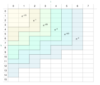
Figure 1. The grid showing which $\nu(k,l)$ need to be caculated for various terms of Edgeworth expansion for a $t$-statistic, with terms indicated as powers of $n$. Combinations of $k$ (rows) and $l$ (columns) needed for a particular term also include all the combinations needed for previous terms as well.

For a generalized two-sample $t$-test, consider mean-zero random variables $X$ and $Y$ with variances $\sigma_{x}^{2}$ and $\sigma_{y}^{2}$ respectively, central moments $\mu_{x,j}$, $\mu_{y,j}$, and a random sample $X_{1},\dotsc,X_{n_{x}},Y_{1},\dotsc,Y_{n_{y}}$. Similarly to the one-sample case, define $\bar{X}=n_{x}^{-1}\sum_{i=1}^{n_{x}}X_{i}$, $\bar{Y}=n_{y}^{-1}\sum_{i=1}^{n_{y}}Y_{i}$, $\bar{X}_{s}=n_{x}^{-1}\sum_{i=1}^{n_{x}}(X_{i}^{2}-\sigma_{x}^{2})$, and $\bar{Y}_{s}=n_{y}^{-1}\sum_{i=1}^{n_{y}}(Y_{i}^{2}-\sigma_{y}^{2})$. As mentioned in section 2, to have a single summary measure representing sample size and to eliminate $n_{x}$ and $n_{y}$ (assuming they are comparable), we introduce $n=(n_{x}+n_{y})/2$, $b_{x}=n/n_{x}$, and $b_{y}=n/n_{y}$. Let $s^{2}=A+B_{x}(\bar{X}_{s}-\bar{X}^{2})+B_{y}(\bar{Y}_{s}-\bar{Y}^{2})$ and let $s^{2}_{\bar{X}-\bar{Y}}=s^{2}/n$ be some estimator of $Var(\bar{X}-\bar{Y})$. In this case there is no immediate interpretation for $s^{2}$ but it is a useful construct that is analogous to the one-sample case. Consider a statistic of the form

(4) $$\hat{\theta}=\frac{\bar{X}-\bar{Y}}{s_{\bar{X}-\bar{Y}}}=\frac{\sqrt{n}(\bar{X}-\bar{Y})}{s}=n^{\frac{1}{2}}(\bar{X}-\bar{Y})\left[A+B_{x}(\bar{X}_{s}-\bar{X}^{2})+B_{y}(\bar{Y}_{s}-\bar{Y}^{2})\right]^{-\frac{1}{2}}$$

Proposition 3.2.

The moments of sampling distribution of $\hat{\theta}$ defined in (4) are given by

$$E\left(\hat{\theta}^{m}\right)= \,n^{\frac{m}{2}}A^{-\frac{m}{2}}\sum_{j=0}^{m}(-1)^{j}{m\choose j}\bigg{[}\rho(m-j,0)\,\tau(j,0)$$

$$\,+\sum_{k=1}^{K}\sum_{i=0}^{\left\lfloor\frac{k}{2}\right\rfloor}(-1)^{i}a_{m,k-i}{k-i\choose i}A^{i-k}\sum_{u=0}^{k-2i}\sum_{v=0}^{i} \!{k-2i\choose u}\!{i\choose v}B_{x}^{(k-i)-(u+v)}B_{y}^{u+v}$$

$$\mkern-15.0mu\times\rho\big{(}m-j+2(i-v),k-2i-u\big{)}\,\tau(j+2v,u)\bigg{]}$$

$$\,+\mathcal{O}\left(n^{-\frac{K+1}{2}}\right),$$

where $a_{m,k}$ is the same as in (3), $\rho(i,j)=E(\bar{X}^{i}\bar{X}_{s}^{j})$, and $\tau(i,j)=E(\bar{Y}^{i}\bar{Y}_{s}^{j})$.

The proof of this Proposition is in Appendix A.

4. Validity of AEE

Let $X$ be a random variable with known moments and cumulants $\kappa_{j}$; set $\kappa_{1}=0$, $\kappa_{2}=1$ without loss of generality. Let $X_{1},\dotsc,X_{n}$ be an i.i.d. sample. First, consider a test statistic as in (2) with a constraint that $A$ and $B$ do not depend on $n$. The function $g(x,y)=n^{\frac{1}{2}}x[A+B(y-x^{2})]^{-\frac{1}{2}}$ is infinitely differentiable in $x$ and $y$, so by the fundamental result of Bhattacharia and Gosh [1] and Hall [30], if $X$ has sufficient number of finite moments, there exists EE of the form

(5) $$P\left(\hat{\theta}<x\right)=F_{\hat{\theta}}(x)=\Phi_{A^{-1}}(x)+\sum_{k=1}^{K}n^{-\frac{k}{2}}q_{k}(x;A,B)\phi_{A^{-1}}(x)+o\left(n^{-\frac{K}{2}}\right),$$

where $q_{k}(x;A,B)$ are some polynomials in $x$ whose coefficients do not depend on $n$ and are expressed in terms of $A$ and $B$. $\Phi_{A^{-1}}(\cdot)$ and $\phi_{A^{-1}}(\cdot)$ denote normal $N(0,A^{-1})$ c.d.f. and p.d.f. In AEE, however, we consider test statistics of the same form but with $A$ and $B$ replaced by $A_{n}$ and $B_{n}$, which do depend on $n$.

Theorem 4.1.

Let $A_{n}=\sum_{j=0}^{\infty}n^{-j}\tilde{a}_{j}$ and $B_{n}=\sum_{j=0}^{\infty}n^{-j}\tilde{b}_{j}$, where $\tilde{a}_{j},\tilde{b}_{j}$ are constants and the series are absolutely convergent. Then, for a test statistic

$$\hat{\theta}_{n}=n^{\frac{1}{2}}\bar{X}\left[A_{n}+B_{n}\left(\bar{X}_{s}-\bar{X}^{2}\right)\right]^{-\frac{1}{2}},$$

there exists AEE of the form

(6) $$P\left(\hat{\theta}_{n}<x\right)=F_{\hat{\theta}_{n}}(x)=\Phi_{A_{n}^{-1}}(x)+\sum_{k=1}^{K}n^{-\frac{k}{2}}q_{k}(x;\,A_{n},B_{n})\phi_{A_{n}^{-1}}(x)+o\left(n^{-\frac{K}{2}}\right).$$

Note that expressions for polynomials $q_{k}(x;\,A_{n},B_{n})$ are the same as those for $q_{k}(x;\,A,B)$ in (5) apart from $A_{n}$, $B_{n}$ replacing $A$, $B$.

The proof (provided in Appendix B) derives the order of finite-term difference between two series that represent cumulants of $\hat{\theta}_{n}$: one that can be used for classic EE and the other - for AEE. Consequently, using the difference $F_{n,K}(x)-\tilde{F}_{n,K}(x)$ and validity of classic EE, we establish the order of $F_{\hat{\theta}_{n}}(x)-\tilde{F}_{n,K}(x)$.

To explicitly relate (6) to the original expression for AEE (1), consider the case where $Var(X)=\sigma^{2}$ and let $r^{2}=\sigma^{2}/A_{n}$. Then, substituting $x^{\prime}=x/\sigma$ for $x$ in (6), we get $\Phi_{A_{n}^{-1}}(x^{\prime})=\Phi(x^{\prime}\sqrt{A_{n}})=\Phi(x^{\prime}/r)$ and $\phi_{A_{n}^{-1}}(x)=\phi(x^{\prime}/r)$.

For a two-sample $t$-test, as previously, we consider a sample $X_{1},\dotsc,X_{n_{x}},Y_{1},\dotsc,Y_{n_{y}}$ and set $n=(n_{x}+n_{y})/2$.

Theorem 4.2.

Let $A_{n}=\sum_{i=0}^{\infty}\left(\tilde{a}_{xi}/n_{x}^{i}+\tilde{a}_{yi}/n_{y}^{i}\right)$, $B_{xn}=\sum_{i=0}^{\infty}\tilde{b}_{xi}/n_{x}^{i}$, and $B_{yn}=\sum_{i=0}^{\infty}\tilde{b}_{yi}/n_{y}^{i}$, where $\tilde{a}_{xi}$, $\tilde{a}_{yi}$, $\tilde{b}_{xi}$, and $\tilde{b}_{yi}$ do not depend on $n_{x}$, $n_{y}$, and the series are absolutely convergent. Then, for a test statistic

$$\hat{\theta}_{n}=n^{\frac{1}{2}}(\bar{X}-\bar{Y})\left[A_{n}+B_{xn}(\bar{X}_{s}-\bar{X}^{2})+B_{yn}(\bar{Y}_{s}-\bar{Y}^{2})\right]^{-\frac{1}{2}}$$

there exists AEE of the form

$$P\left(\hat{\theta}_{n}<x\right)=F_{\hat{\theta}_{n}}(x)=\Phi_{A_{n}^{-1}}(x)+\sum_{k=1}^{K}n^{-\frac{k}{2}}q_{k}(x;\,A_{n},B_{xn},B_{yn})\phi_{A_{n}^{-1}}(x)+o\left(n^{-\frac{K}{2}}\right).$$

The proof of this Theorem is in Appendix B.

5. Results

In this section, we provide expressions for AEE at different levels of generalization. Recall that in the process of obtaining EE, cumulants $\kappa_{\hat{\theta},j}$ of sampling distribution are expressed as power series in $n^{-1/2}$. As seen in, for example, [30], [39]:

$$\kappa_{\hat{\theta},j}=n^{-\frac{j-2}{2}}\left(k_{j,1}+n^{-1}k_{j,2}+n^{-2}k_{j,3}+\dotsb\right),\qquad j\geqslant 1.$$

Once $k_{j,l}$ are obtained, they can be used to calculate polynomials $q_{k}(x;r)$ in (1), together with Hermite polynomials. Expressions for $q_{k}$ as functions of $k_{j,l}$ can be used for AEE of any test statistic. Next, for one- and two-sample generalized $t$-statistics, we look at $k_{j,l}$ as functions of $\mu_{j}$, $A_{n}$, and $B_{n}$ (going forward, we omit the subscript $n$ for brevity). Finally, we provide $A$, $B$, and $r^{2}$ for some commonly used versions of these statistics as well as for moderated $t$-statistics based on empirical Bayes methods [38]). In addition, for the simplest special case of an ordinary one-sample $t$-statistic with naïve biased and unbiased variance estimators, this nested chain of expressions reduces to a nice short form where $q_{k}(x;r)$ are given in terms of standardized cumulants $\lambda_{j}$ (provided here for the 4-term AEE). For these particular statistics, such form is useful for calculations and also allows for an illuminating comparison with known expressions for standardized mean. 2-term EE of this kind is found in [29, 30].

5.1. General case

For a given test statistic, first few polynomials $q_{k}(x;r)$ of AEE (1) are given by

$$q_{1}(x;r) =-\frac{1}{6\,r^{3}}\,k_{3,1}\,He_{2}\left(\frac{x}{r}\right)-\frac{1}{r}\,k_{1,2}$$

$$q_{2}(x;r)= -\frac{1}{72\,r^{6}}\,k_{3,1}^{2}\,He_{5}\left(\frac{x}{r}\right)-\frac{1}{24\,r^{4}}\,{\left(4\,k_{1,2}k_{3,1}+k_{4,1}\right)}\,{He}_{3}\left(\frac{x}{r}\right)$$

$$-\frac{1}{2\,r^{2}}\,{\left(k_{1,2}^{2}+k_{2,2}\right)}\,{He}_{1}\left(\frac{x}{r}\right),$$

where $He_{j}(x)$ are probabilists’ Hermite polynomials. Since $k_{j,l}$’s do not depend on $x$, this approach is especially useful if $\tilde{F}_{n,K}(x)$ needs to be calculated for many values of $x$.

For generalized one- and two-sample $t$-statistics, we show some lower order $k_{j,l}$’s in this paper; all $k_{j,l}$’s needed for fifth order AEE, as well as remaining general case $q_{k}(x;r)$, can be found in the Sage notebook and edgee R package [41]. Note that $k_{2,1}=r^{2}$.

For the one-sample $t$-statistic:

$$k_{1,2}=-\frac{B\mu_{3}}{2A^{\frac{3}{2}}}$$

$$k_{1,3}=-\frac{6(8\mu_{2}\mu_{3}-\mu_{5})AB^{2}-15(\mu_{2}^{2}\mu_{3}-\mu_{3}\mu_{4})B^{3}-8A^{2}B\mu_{3}}{16A^{\frac{7}{2}}}$$

$$k_{2,1}=\frac{\mu_{2}}{A}$$

$$k_{2,2}=\frac{4(4\mu_{2}^{2}-\mu_{4})AB-(4\mu_{2}^{3}-7\mu_{3}^{2}-4\mu_{2}\mu_{4})B^{2}}{4A^{3}}$$

$$k_{3,1}=-\frac{(3B\mu_{2}-A)\mu_{3}}{A^{\frac{5}{2}}}$$

$$k_{4,1}=-\frac{(3\mu_{2}^{2}-\mu_{4})A^{2}-6(3\mu_{2}^{3}-\mu_{3}^{2}-\mu_{2}\mu_{4})AB+3(\mu_{2}^{4}-6\mu_{2}\mu_{3}^{2}-\mu_{2}^{2}\mu_{4})B^{2}}{A^{4}}$$

The two-sample $t$-statistic:

$$k_{1,2}=-\frac{B_{x}b_{x}\mu_{x,3}-B_{y}b_{y}\mu_{y,3}}{2A^{\frac{3}{2}}}$$

$$k_{2,1}=\frac{b_{x}\mu_{x,2}+b_{y}\mu_{y,2}}{A}$$

$$k_{2,2}= -\frac{4B_{x}^{2}b_{x}^{2}\mu_{x,2}^{3}+4B_{y}^{2}b_{x}b_{y}\mu_{x,2}\mu_{y,2}^{2}+4B_{y}^{2}b_{y}^{2}\mu_{y,2}^{3}-4B_{x}^{2}b_{x}^{2}\mu_{x,2}\mu_{x,4}}{4A^{3}}$$

$$+\frac{14B_{x}B_{y}b_{x}b_{y}\mu_{x,3}\mu_{y,3}-7B_{x}^{2}b_{x}^{2}\mu_{x,3}^{2}-7B_{y}^{2}b_{y}^{2}\mu_{y,3}^{2}}{4A^{3}}$$

$$-\frac{4A(B_{x}b_{x}^{2}(4\mu_{x,2}^{2}-\mu_{x,4})+B_{y}b_{y}^{2}(4\mu_{y,2}^{2}-\mu_{y,4})+(B_{x}b_{x}b_{y}+B_{y}b_{x}b_{y})\mu_{x,2}\mu_{y,2})}{4A^{3}}$$

$$+\frac{4(B_{x}^{2}b_{x}b_{y}\mu_{x,2}^{2}-B_{x}^{2}b_{x}b_{y}\mu_{x,4})\mu_{y,2}-4(B_{y}^{2}b_{x}b_{y}\mu_{x,2}+B_{y}^{2}b_{y}^{2}\mu_{y,2})\mu_{y,4}}{4A^{3}}$$

$$k_{3,1}= -\frac{(3B_{x}b_{x}^{2}\mu_{x,2}+3B_{x}b_{x}b_{y}\mu_{y,2}-Ab_{x}^{2})\mu_{x,3}-(3B_{y}b_{x}b_{y}\mu_{x,2}+3B_{y}b_{y}^{2}\mu_{y,2}-Ab_{y}^{2})\mu_{y,3}}{A^{\frac{5}{2}}}$$

Thus $r^{2}=\sigma^{2}/A$ for a one-sample $t$-statistic and $r^{2}=(b_{x}\sigma_{x}^{2}+b_{y}\sigma_{y}^{2})/A$ for a two-sample $t$-statistic.

5.2. Examples of specific $t$-tests

Statistics we consider here are a set of commonly used ordinary $t$-statistics as well as moderated statistics that incorporate more complex variance estimators [38]. For the first set, we look at one-sample $t$-statistics with naïve biased and unbiased variance estimators (with Bessel’s correction), two-sample $t$-statistic that assumes equal variances between two groups and uses pooled (unbiased) variance estimator, and Welch $t$-tests that do not assume equal variances - with both naïve biased and unbiased variance estimators. For a higher-order approach to two-sample equal variance test, we also assume equality of higher moments of distributions of $X$ and $Y$. Note that these assumptions allow for a more efficient estimator, so there is an advantage to using pooled variance if the equality assumption is reasonable.

Moderated $t$-statistic, which uses empirical Bayes approach, became a great practical tool widely used in high-dimensional data analysis. In this case, the normalizing factor is a posterior variance for a feature $g$ (e.g. a gene) that incorporates prior information. The method uses a hierarchical model, in which two hyperparameters $s_{0}^{2}$ and $d_{0}$ are estimated from the data that has many features. Estimators for these parameters have a closed form and are sufficiently stable due to the fact that high dimensionality provides extensive information from which only two hyperparameters are estimated - even when the number of replicates (sample size) is small. This allows us to treat $s_{0}^{2}$ and $d_{0}$ as constants in deriving AEE. Posterior variance $\tilde{s}_{g}^{2}$ for a feature $g$ is a linear combination of $s_{0}^{2}$ and a sample/residual variance $s_{g}^{2}$: $\displaystyle{\tilde{s}_{g}^{2}=\frac{d_{0}s_{0}^{2}+d_{g}{s_{g}^{2}}}{d_{0}+d_{g}}}$, where $d_{0}$ and $d_{g}$ are prior and residual degrees of freedom. Because of that, moderated $t$-statistic can also be viewed as a generalization for any scaled mean-based statistic as it can be reduced to either standardized ($d_{g}=0$) or studentized ($d_{0}=0$) version. If data are distributed normally, moderated $t$-statistic follows a $t$-distribution with augmented ($d_{g}+d_{0}$) degrees of freedom.

Let $C=\frac{n}{n-1}$ for one-sample tests and $C_{x}=\frac{n_{x}}{n_{x}-1}$, $C_{y}=\frac{n_{y}}{n_{y}-1}$, and $C_{xy}=\frac{n_{x}+n_{y}}{n_{x}+n_{y}-2}=\frac{n}{n-1}$ for two-sample tests (recall that $n=\frac{n_{x}+n_{y}}{2}$, $b_{x}=\frac{n}{n_{x}}$, and $b_{y}=\frac{n}{n_{y}}$). Generalized expressions for variance estimators $s^{2}=A+B(\bar{X}_{s}-\bar{X}^{2})$ (one-sample) and $s^{2}=A+B_{x}(\bar{X}_{s}-\bar{X}^{2})+B_{y}(\bar{Y}_{s}-\bar{Y}^{2})$ (two-sample) allow us to easily extract $A$ and $B$ for each particular case. Note that for moderated $t$-statistics $d_{g}=n-1$ for one-sample and $d_{g}=n_{x}+n_{y}-2$ for two-sample tests (and thus $C_{xy}d_{g}=n_{x}+n_{y}=2n$).

Table 1 provides expressions for $A$, $B$, and $r^{2}$ for various one-sample $t$-statistics, $\hat{\theta}=\sqrt{n}\bar{X}/s$. For two-sample versions, $\hat{\theta}=\sqrt{n}(\bar{X}-\bar{Y})/s$, we introduce some short-hand notations: let $s_{x}^{2}=n^{-1}\sum_{i=1}^{n_{x}}(X_{i}-\bar{X})^{2}$, $s_{y}^{2}=n^{-1}\sum_{i=1}^{n_{y}}(Y_{i}-\bar{Y})^{2}$, and $s_{xy}^{2}=(n_{x}+n_{y})^{-1}\big{(}\sum_{i=1}^{n_{x}}(X_{i}-\bar{X})^{2}+\sum_{i=1}^{n_{y}}(Y_{i}-\bar{Y})^{2}\big{)}$ be naïve biased estimators of $\sigma_{x}^{2}$, $\sigma_{y}^{2}$, and $\sigma^{2}=\sigma_{x}^{2}=\sigma_{y}^{2}$ respectively. Table 2 shows expressions for $A$, $B_{x}$, $B_{y}$, and $r^{2}$ for several two-sample $t$-tests.

type	variance estimator	$s^{2}$	$A$	$B$	$r^{2}$
ordinary	biased	$\displaystyle{\frac{1}{n}\sum_{i=1}^{n}(X_{i}-\bar{X})^{2}}$	$\sigma^{2}$	$1$	$1$
ordinary	unbiased	$\displaystyle{\frac{1}{n-1}\sum_{i=1}^{n}(X_{i}-\bar{X})^{2}}$	$C\sigma^{2}$	$C$	$\displaystyle{\frac{1}{C}}$
moderated	posterior	$\displaystyle{\frac{d_{0}s_{0}^{2}+\sum_{i=1}^{n}(X_{i}-\bar{X})^{2}}{d_{0}+n-1}}$	$\displaystyle{\frac{d_{0}s_{0}^{2}+n\sigma^{2}}{d_{0}+n-1}}$	$\displaystyle{\frac{n}{d_{0}+n-1}}$	$\displaystyle{\frac{d_{0}+n-1}{d_{0}s_{0}^{2}/\sigma^{2}+n}}$

Table 1. One-sample statistics

type	variance estimator	$s^{2}$	$A$	$B_{x}$	$B_{y}$	$r^{2}$
Welch	biased	$b_{x}s_{x}^{2}+b_{y}s_{y}^{2}$	$b_{x}\sigma_{x}^{2}+b_{y}\sigma_{y}^{2}$	$b_{x}$	$b_{y}$	$1$
Welch	unbiased	$C_{x}b_{x}s_{x}^{2}+C_{y}b_{y}s_{y}^{2}$	$C_{x}b_{x}\sigma_{x}^{2}+C_{y}b_{y}\sigma_{y}^{2}$	$C_{x}b_{x}$	$C_{y}b_{y}$	$\displaystyle{\frac{b_{x}\sigma_{x}^{2}+b_{y}\sigma_{y}^{2}}{C_{x}b_{x}\sigma_{x}^{2}+C_{y}b_{y}\sigma_{y}^{2}}}$
ordinary	pooled unbiased	$C_{xy}(b_{x}+b_{y})s_{xy}^{2}$	$C_{xy}(b_{x}+b_{y})\sigma^{2}$	$C_{xy}b_{y}$	$C_{xy}b_{x}$	$\displaystyle{\frac{1}{C_{xy}}}$
moderated	posterior	$\displaystyle{\frac{(b_{x}+b_{y})(d_{0}s_{0}^{2}+C_{xy}d_{g}s_{xy}^{2})}{d_{0}+d_{g}}}$	$\displaystyle{\frac{(b_{x}+b_{y})(d_{0}s_{0}^{2}+C_{xy}d_{g}\sigma^{2})}{d_{0}+d_{g}}}$	$\displaystyle{\frac{C_{xy}d_{g}b_{y}}{d_{0}+d_{g}}}$	$\displaystyle{\frac{C_{xy}d_{g}b_{x}}{d_{0}+d_{g}}}$	$\displaystyle{\frac{d_{0}+d_{g}}{d_{0}s_{0}^{2}/\sigma^{2}+C_{xy}d_{g}}}$

Table 2. Two-sample statistics

5.3. Special case: one-sample ordinary $t$

When the scaling factor is naïve biased variance estimator $s_{b}^{2}$, classic EE coincide with AEE ($r^{2}=1$). Polynomials representing a $4$-term expansion are written in terms of $\lambda_{j}=\kappa_{j}/\sigma^{j}$, which allows for a comparison with traditional expressions for standardized mean.

$$q_{1}(x;1) =\,\frac{1}{6}\,\lambda_{3}\,{\left(2\,x^{2}+1\right)}$$

$$q_{2}(x;1) =\,\frac{1}{12}\,\lambda_{4}\,{\left(x^{3}-3\,x\right)}-\frac{1}{18}\,\lambda_{3}^{2}\,{\left(x^{5}+2\,x^{3}-3\,x\right)}-\frac{1}{4}\,{\left(x^{3}+3\,x\right)}$$

$$q_{3}(x;1)= \,-\frac{1}{40}\,\lambda_{5}\,{\left(2\,x^{4}+8\,x^{2}+1\right)}-\frac{1}{144}\,\lambda_{3}\lambda_{4}\,{\left(4\,x^{6}-30\,x^{4}-90\,x^{2}-15\right)}$$

$$\,+\frac{1}{1296}\,\lambda_{3}^{3}\,{\left(8\,x^{8}+28\,x^{6}-210\,x^{4}-525\,x^{2}-105\right)}$$

$$\,+\frac{1}{24}\,\lambda_{3}\,{\left(2\,x^{6}-3\,x^{4}-6\,x^{2}\right)}$$

$$q_{4}(x;1)=\, -\frac{1}{90}\,\lambda_{6}\,{\left(2\,x^{5}-5\,x^{3}-15\,x\right)}+\frac{1}{60}\,\lambda_{3}\lambda_{5}\,{\left(x^{7}+8\,x^{5}-5\,x^{3}-30\,x\right)}$$

$$-\frac{1}{288}\,\lambda_{4}^{2}\,{\left(x^{7}-21\,x^{5}+33\,x^{3}+111\,x\right)}$$

$$+\frac{1}{216}\,\lambda_{3}^{2}\lambda_{4}\,{\left(x^{9}-12\,x^{7}-90\,x^{5}+36\,x^{3}+261\,x\right)}$$

$$-\frac{1}{1944}\,\lambda_{3}^{4}\,{\left(x^{11}+5\,x^{9}-90\,x^{7}-450\,x^{5}+45\,x^{3}+945\,x\right)}$$

$$+\frac{1}{48}\,\lambda_{4}\,{\left(x^{7}-7\,x^{5}+9\,x^{3}+21\,x\right)}-\frac{1}{72}\,\lambda_{3}^{2}\,{\left(x^{9}-6\,x^{7}-12\,x^{5}-18\,x^{3}-9\,x\right)}$$

$$-\frac{1}{96}\,{\left(3\,x^{7}+5\,x^{5}+7\,x^{3}+21\,x\right)}$$

These expressions can be also used for the most common $t$-statistic with unbiased variance estimator (if $X$ is distributed normally, this statistic has Student’s $t$-distribution). In that particular case, $q_{k}(x;r)=q_{k}(x/r;1)=q_{k}(\sqrt{\frac{n}{n-1}}\,x;1)$.

6. Illustration of Higher-Order Approximations

To provide an illustration for higher-order approximations to the distribution of a $t$-statistic, we consider an example with a small sample ($n=10$) of i.i.d. centered gamma distributed random variables with shape parameter $k=3$: $X\sim\Gamma(3,1)-3$ and two versions of an ordinary $t$-statistic - with biased $s_{b}^{2}$ and unbiased $s_{unb}^{2}$ variance estimators: $t_{1}=n^{1/2}\bar{X}/s_{b}$ and $t_{2}=n^{1/2}\bar{X}/s_{unb}$. Figure 2 displays AEE of up to fifth order ($0-4$-term expansions) for $t_{1}$ and $t_{2}$ along with their respective true sampling distributions; known values of $\lambda_{j}$ are used for the expansions.

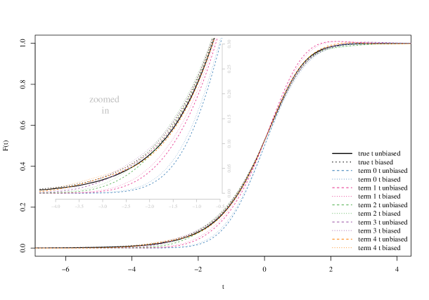
Figure 2. Sampling distributions of an ordinary $t$-statistic with biased and unbiased variance estimators and their AEE approximations. $X\sim\Gamma(3,1)-3$, $n=10$.

Edgeworth expansions are not probability functions and do not have their properties - they are not necessarily monotonic everywhere and might not be bounded by $0$ and $1$. This irregular behavior is usually localized in the thinner tail of the distribution and therefore EE are not very helpful there; it is clearly seen in the second order approximation (term $1$) in the graph. We focus on the thicker left tail where inference based on the first order approximation would be anti-conservative (discussed in more detail in Section 7). The difference between the normal approximation (term $0$) and the true distribution is quite striking; subsequent orders improve approximation considerably. It appears that the third order is already fairly close to the truth; however, as we move away from the center and into the far tail, this approximation gets further from the distribution and higher order terms come into play proving the value of Edgeworth expansions of the orders beyond the second and even third. This indicates how AEE can be used to adjust inference for detected departures from normality in the tails of a sampling distribution.

7. Discussion

Generalized results for one- and two-sample $t$-statistics offer a possibility of using AEE in a variety of data analysis scenarios and statistical procedures. As Figure 2 demonstrates, first order approximation may result in anti-conservative inference and consequently lack of error rate control [44]. These issues arise when the tails of a sampling distribution are thick, which is where EE behave nicely providing increasingly closer approximations. Conversely, non-monotoniciy and values beyond $[0,1]$ discussed in Section 6 can occur in the thinner tails where traditional first order approximation provides conservative inference and thus can be reliably used. For practical applications, this EE tail behavior means that some kind of “tail diagnostic” would need to be performed in order to determine a usable order of approximation for each side. In fact, the “irregularity” can be approached with “it’s not a bug, it’s a feature” attitude: if the sample is representative, AEE tail diagnostic can provide information about sampling distribution, specifically on symmetry and tail thickness. Then, each subsequent order can be guaranteed to be more conservative than the previous one - for example, in the context of hypothesis testing, the null hypothesis would be rejected with more certainty as the order increases. Another issue to be considered when adapting AEE to data analysis is that since the true central moments of the data generating distribution are not known, they would be substituted with estimates. As higher moments are more sensitive to the choice of estimators (e.g. naïve biased vs unbiased), estimators’ behavior and its effect on the performance of higher-order inference would need to be explored.

AEE for ordinary one-sample $t$-statistics (Section 5.3) and their comparison with EE for a standardized mean capture some key differences between standardized and studentized statistics and underline important features of $t$-statistic’s distribution. To get some insight into these differences, we can turn to the Student’s $t$-distribution with $n-1$ degrees of freedom, which was derived as a distribution of a $t$-statistic for a sample of $n$ i.i.d. normally distributed random variables. Its derivation relies on a specific property unique to Gaussian distribution: independence of sample mean and sample variance. Without normality, this is no longer the case, which can be easily seen with asymmetric distributions. Consider a distribution of $X$ that is skewed to the right, with the thin left and thick right tails. While the distribution of standardized mean (scaled by a constant) is also skewed to the right, the distribution of studentized mean (scaled by a random variable) is, in contrast, skewed to the left (Fig 3(a)). The reason for the “flip” stems from the fact that observations that contribute to a greater sample average, coming from the thicker tail, have greater dispersion as well, thus resulting in a smaller value for $t$-statistic. Moreover, as can be seen in Fig 3(b), the difference between thicker and thinner tails appears to be even more pronounced than that of a ratio with assumed indepence (obtained with permutation/random pairings of averages and standard errors from different samples). EE for studentized mean do not assume independence of sample mean and sample variance; truncated series approach the correct shape of the distribution (as seen in Figure 2).

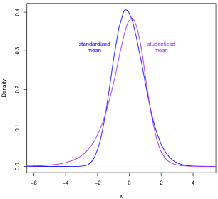
(a) Standardized mean $\bar{X}/s$ vs
studentized $\bar{X}/\sigma$

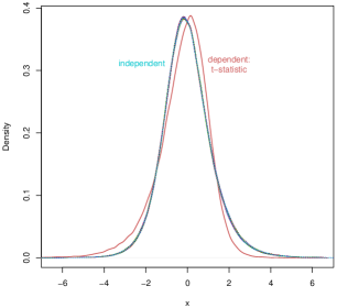
(b) $t$-statistic (dependent) vs
$\bar{X}/s$: $\bar{X}\perp s$

Figure 3. Distribution of scaled means, $X\sim\Gamma(3,1)-3$, $n=10$.

Another feature of these expansions in contrast with the ones for standardized statistics is the cumulant order “inconsistency” inside the polynomials for expansion terms. To see that, first consider a standardized mean $\hat{\theta}=\sqrt{n}(\bar{X}-E(X))/\sigma$. For cumulants $\kappa_{\hat{\theta},j}$ of sampling distribution and $\kappa_{j}$ of distribution of $X$, $\kappa_{\hat{\theta},j}=n^{-\frac{j-2}{2}}\kappa_{j}$ since $\varphi_{\hat{\theta}}(t)=\big{[}\varphi(t/\sqrt{n})\big{]}^{n}$, where $\varphi_{\hat{\theta}}$ and $\varphi$ are characteristic functions of $\hat{\theta}$ and $X$ respectively [30]. The consequence of that is that standardized cumulants $\lambda_{j}$ are associated with $n^{-\frac{j-2}{2}}$ and all the terms of EE polynomials respect that order - e.g. factors of the third term polynomial $q_{3}$ are $\lambda_{5}$, $\lambda_{3}\lambda_{4}$, and $\lambda_{3}^{3}$. That cumulant relation is not true for a studentized mean, which is reflected in EE. Again, reference to normal distribution might provide some intuition for the effect of this difference. Consider $X\sim N(\mu,\sigma^{2})$ and $\hat{\theta}=\sqrt{n}(\bar{X}-\mu)/s\sim t_{n-1}$. Then $\lambda_{j}=0$, $j=3,\dotsc$ and $q_{1}=q_{3}=\dotsb=0$. Even term polynomials ($q_{2},q_{4},\dotsc$) have remaining non-zero terms that make the tails thicker, consistent with the fact that Student’s $t$-distribution has non-unit variance and thicker tails than normal. For non-normal distributions, polynomial terms that contain cumulants but are not of a “regular” order are likely to also contribute to thickness of the tails though it is harder to assess.

Student’s $t$, while not a sampling distribution for any random variable but normal (and not a limit distribution), can be useful in exploring far tails of distributions of studentized mean-based statistics and an effect of sample size on associated critical values [44] in, for example, high-dimensional data analysis with multiple comparisons. In fact, it is routinely used in practice, with stated but not always warranted normality assumption to justify its use; it can be argued that it still provides useful approximation to sampling distribution for large deviations and small sample size ([45]). Combining higher-order inference approach of AEE with $t$-distribution for challenging extreme tail estimation could be another fruitful direction for achieving more reliable inference.

Appendix A Proofs of Propositions

Proof of Proposition 3.1.

(7) $$\hat{\theta}^{m}=n^{\frac{m}{2}}A^{-\frac{m}{2}}\bar{X}^{m}\,(1+\gamma_{1}-\gamma_{2})^{-\frac{m}{2}}=n^{\frac{m}{2}}A^{-\frac{m}{2}}\bar{X}^{m}\left[1+\sum_{k=1}^{\infty}a_{m,k}(\gamma_{1}-\gamma_{2})^{k}\right],$$

where $\gamma_{1}=A^{-1}B\bar{X}_{s}=\mathcal{O}\left(n^{-1/2}\right)$, $\gamma_{2}=A^{-1}B\bar{X}^{2}=\mathcal{O}\left(n^{-1}\right)$, and $a_{m,k}$ as defined in (3).

From Taylor expansion of $(1+\gamma_{1}-\gamma_{2})^{-\frac{m}{2}}$ and, subsequently, from $(\gamma_{1}-\gamma_{2})^{k}$ (7) we only need the terms with factors up to $n^{-\frac{K}{2}}$. Knowing the orders of $\gamma_{1}$ and $\gamma_{2}$ does not only allow us to use Taylor expansion in the first place, it also provides a tool to keep only the relevant terms of the expansion.

Start with grouping the terms by orders (powers of $n^{-\frac{1}{2}}$):

$${\left(1+\gamma_{1}-\gamma_{2}\right)}^{-\frac{m}{2}} = \,1+\sum_{k=1}^{\infty}a_{m,k}\sum_{i=0}^{k}{k\choose i}(-1)^{i}\,\gamma_{1}^{k-i}\,\gamma_{2}^{i}$$

$$= \,\Bigg{(}1+\sum_{k=1}^{\infty}\Bigg{[}a_{m,k}{k\choose 0}\gamma_{1}^{k}\,\gamma_{2}^{0}-a_{m,k-1}{k-1\choose 1}\gamma_{1}^{k-2}\,\gamma_{2}^{1}+a_{m,k-2}{k-2\choose 2}\gamma_{1}^{k-4}\,\gamma_{2}^{2}$$

$$\;\;\;\;-\dotsb+\begin{cases}\,a_{m,\frac{k}{2}}(-1)^{\frac{k}{2}}\,\displaystyle{{\frac{k}{2}\choose\frac{k}{2}}}\gamma_{1}^{0}\,\gamma_{2}^{\frac{k}{2}}\,\Bigg{]}\Bigg{)}&\text{ - for even }k\\[15.00002pt] \,a_{m,\frac{k+1}{2}}(-1)^{\frac{k-1}{2}}\displaystyle{{\frac{k+1}{2}\choose\frac{k-1}{2}}}\gamma_{1}^{1}\,\gamma_{2}^{\frac{k-1}{2}}\,\Bigg{]}\Bigg{)}&\text{ - for odd }k\end{cases}$$

$$= \,1+\sum_{k=1}^{\infty}\sum_{i=0}^{\left\lfloor\frac{k}{2}\right\rfloor}a_{m,k-i}(-1)^{i}{k-i\choose i}\gamma_{1}^{k-2i}\,\gamma_{2}^{i}$$

From this, we can pick $K$ terms and get

$$\hat{\theta}^{m} =\,n^{\frac{m}{2}}A^{-\frac{m}{2}}\bar{X}^{m}\left[\,1+\sum_{k=1}^{K}\sum_{i=0}^{\left\lfloor\frac{k}{2}\right\rfloor}a_{m,k-i}(-1)^{i}{k-i\choose i}\gamma_{1}^{k-2i}\,\gamma_{2}^{i}\,\right]+\mathcal{O}\left(n^{-\frac{K+1}{2}}\right)$$

Then

$$E\left(\hat{\theta}^{m}\right)=n^{\frac{m}{2}}A^{-\frac{m}{2}}\Bigg{[}\,\rho(m,0)+\sum_{k=1}^{K}\sum_{i=0}^{\left\lfloor\frac{k}{2}\right\rfloor}a_{m,k-i}(-1)^{i}{k-i\choose i}\,\frac{B^{k-i}}{A^{k-i}}\,\rho(m+2i,k-2i)\,\Bigg{]}+\mathcal{O}\left(n^{-\frac{K+1}{2}}\right)$$

∎

Proof of Proposition 3.2.

Applying the same argument for truncation and leaving only terms of relevant orders as in the one-sample case, we get the expression:

(8) $$\hat{\theta}^{m}=n^{\frac{m}{2}}A^{-\frac{m}{2}}(\bar{X}-\bar{Y})^{m}\left[1+\sum_{k=1}^{K}\sum_{i=0}^{\left\lfloor\frac{k}{2}\right\rfloor}(-1)^{i}a_{m,k-i}{k-i\choose i}\gamma_{1}^{k-2i}\,\gamma_{2}^{i}\right]+\mathcal{O}\left(n^{-\frac{K+1}{2}}\right)$$

where $\gamma_{1}=A^{-1}(B_{x}\bar{X}_{s}+B_{y}\bar{Y}_{s})$, $\gamma_{2}=A^{-1}(B_{x}\bar{X}^{2}+B_{y}\bar{Y}^{2})$, and $a_{m,k}$ is the same as in (3). It is straightforward to show that $\gamma_{1}=\mathcal{O}(n^{-\frac{1}{2}})$ and $\gamma_{2}=\mathcal{O}(n^{-1})$.

For the expectation, we need to expand $\gamma_{1}^{k}\,\gamma_{2}^{l}$:

$$\gamma_{1}^{k}\,\gamma_{2}^{l}=\frac{1}{A^{k+l}}\sum_{i=0}^{k}\sum_{j=0}^{l}{k\choose i}{l\choose j}B_{x}^{(k+l)-(i+j)}B_{y}^{i+j}\bar{X}^{2(l-j)}\bar{X}_{s}^{k-i}\,\bar{Y}^{2j}\,\bar{Y}_{s}^{i}.$$

$$E\left(\hat{\theta}^{m}\right)= \,n^{\frac{m}{2}}A^{-\frac{m}{2}}\sum_{j=0}^{m}(-1)^{j}{m\choose j}\bigg{[}\rho(m-j,0)\,\tau(j,0)+\sum_{k=1}^{K}\sum_{i=0}^{\left\lfloor\frac{k}{2}\right\rfloor}(-1)^{i}a_{m,k-i}{k-i\choose i}A^{i-k}$$

$$\phantom{+}\;\times\sum_{u=0}^{k-2i}\sum_{v=0}^{i}{k-2i\choose u}\!{i\choose v}B_{x}^{(k-i)-(u+v)}B_{y}^{u+v}\rho\big{(}m-j+2(i-v),k-2i-u\big{)}\,\tau(j+2v,u)\bigg{]}$$

$$+\mathcal{O}\left(n^{-\frac{K+1}{2}}\right)$$

∎

Appendix B Proofs of Theorems

Proof of Theorem 4.1.

We can write $\hat{\theta}_{n}$ in the following way:

$$\hat{\theta}_{n}=n^{\frac{1}{2}}\bar{X}\,A^{-\frac{1}{2}}\,(1+b\gamma)^{-\frac{1}{2}},\text{ where}$$

$b=B/A$, $\gamma=\bar{X}_{s}-\bar{X}^{2}$, $\bar{X}=n^{-1}\sum_{i=1}^{n}X_{i}$, and $\bar{X}_{s}=n^{-1}\sum_{i=1}^{n}X_{i}^{2}-\mu_{2}$.

$$\hat{\theta}_{n}^{m}=n^{\frac{m}{2}}\bar{X}^{m}A^{-\frac{m}{2}}(1+b\gamma)^{-\frac{m}{2}}=n^{\frac{m}{2}}A^{-\frac{m}{2}}\sum_{k=0}^{\infty}b^{k}a_{m,k}\sum_{i=0}^{k}{k\choose i}(-1)^{i}\bar{X}_{s}^{k-i}\bar{X}^{2i+m},$$

where $a_{m,k}$ is the same as in (3). Taking expectation, we obtain

$$\mu_{\hat{\theta},m}=E\left(\hat{\theta}_{n}^{m}\right)=n^{\frac{m}{2}}A^{-\frac{m}{2}}\sum_{k=0}^{\infty}b^{k}a_{m,k}\sum_{i=0}^{k}{k\choose i}(-1)^{i}\rho(2i+m,k-i).$$

It can be shown that $\rho(u,w)=\sum_{v=\left\lceil\frac{u+w}{2}\right\rceil}^{u+w-1}\frac{1}{n^{v}}\beta(u,w,v)$, where $\beta(u,w,v)$ does not depend on $n$ and only depends on moments of $X$. Then

$$\mu_{\hat{\theta},m}=n^{\frac{m}{2}}A^{-\frac{m}{2}}\sum_{k=0}^{\infty}b^{k}a_{m,k}\sum_{i=0}^{k}{k\choose i}(-1)^{i}\sum_{v=\left\lceil\frac{m+k+i}{2}\right\rceil}^{m+k+i-1}\frac{1}{n^{v}}\beta(2i+m,k-i,v).$$

Switch the order of summation, summing over $v$ first and over $k$ second:

$$\mu_{\hat{\theta},m}=A^{-\frac{m}{2}}n^{-\frac{1}{2}\delta(m)}\sum_{v=0}^{\infty}\frac{1}{n^{v}}\sum_{k=k_{1}}^{k_{2}}b^{k}\tilde{g}(k,v;\,m),$$

where $\delta(m)=m\mod 2$, $k_{1}=max\left(0,\left\lceil\frac{1}{2}\left(v-\left\lfloor\frac{m}{2}\right\rfloor+1\right)\right\rceil\right)$, $k_{2}=2v+\delta(m)$, $\tilde{g}(k,v;\,m)=a_{m,k}\sum_{i=i_{1}}^{i_{2}}{k\choose i}(-1)^{i}\beta\big{(}2i+m,k-i,v+\left\lceil\frac{m}{2}\right\rceil\big{)}$ with $i_{1}=max\big{(}0,v-\left\lfloor\frac{m}{2}\right\rfloor+1-k\big{)}$ and $i_{2}=min(k,2v+\delta(m)-k)$; $\tilde{g}(k,v;\,m)$ does not depend on $n$. If $k_{1}>0$, we can sum over $k$ starting from $k=0$ and set $\tilde{g}(k,v;\,m)=0$ if $0\leqslant k<k_{1}$.

As we only need a finite number of terms for the expansions, we consider the finite sum in the moments as well:

$$\mu_{\hat{\theta},m}=A^{-\frac{m}{2}}n^{-\frac{1}{2}\delta(m)}\left[\sum_{v=0}^{V}\frac{1}{n^{v}}\sum_{k=0}^{2v+\delta(m)}b^{k}\,\tilde{g}(k,v;\,m)+\mathcal{O}\left(n^{-(V+1)}\right)\right].$$

Next we look at the moment products. Using an induction-like argument, we can show that

$$\mu_{\hat{\theta},m_{1}}^{l_{1}}\mu_{\hat{\theta},m_{2}}^{l_{2}}\dotsm\mu_{\hat{\theta},m_{d}}^{l_{d}}= \,A^{-\frac{1}{2}\sum_{i=1}^{d}l_{i}m_{i}}n^{-\frac{1}{2}\sum_{i=1}^{d}l_{i}\delta(m_{i})}$$

(9) $$\times\left[\sum_{v=0}^{V}\frac{1}{n^{v}}\sum_{k=0}^{2v+\sum_{i=1}^{d}l_{i}\delta(m_{i})}b^{k}g(k,v;\,\boldsymbol{m},\boldsymbol{l})+\mathcal{O}\left(n^{-(V+1)}\right)\right],$$

where $\boldsymbol{m}=(m_{1},\dotsc,m_{d})$, $\boldsymbol{l}=(l_{1},\dotsc,l_{d})$, and $g(k,v;\,\boldsymbol{m},\boldsymbol{l})$ does not depend on $n$. Indeed, the base case is $\boldsymbol{m}=(m)$, $\boldsymbol{l}=(1)$; then $g(k,v;\,\boldsymbol{m},\boldsymbol{l})=\tilde{g}(k,v;\,m)$ does not depend on $n$. Next, consider $\boldsymbol{m}=(m_{1},\dotsc,m_{d})$, $\boldsymbol{l}=(l_{1},\dotsc,l_{d})$, $\boldsymbol{k}=(k_{1},\dotsc,k_{g})$, $\boldsymbol{j}=(j_{1},\dotsc,j_{g})$, and $g(k,v;\,\boldsymbol{m},\boldsymbol{l})$, $g(k,v;\,\boldsymbol{k},\boldsymbol{j})$ that do not depend on $n$ and find $\mu_{\hat{\theta},m_{1}}^{l_{1}}\dotsm\mu_{\hat{\theta},m_{d}}^{l_{d}}\mu_{\hat{\theta},k_{1}}^{j_{1}}\dotsm\mu_{\hat{\theta},k_{g}}^{j_{g}}$. By simple multiplication, gathering the terms by powers of $1/n$, and adding a finite number of resulting higher-order terms to $\mathcal{O}\left(n^{-(V+1)}\right)$, we get

$$\mu_{\hat{\theta},m_{1}}^{l_{1}}\dotsm\mu_{\hat{\theta},m_{d}}^{l_{d}}\mu_{\hat{\theta},k_{1}}^{j_{1}}\dotsm\mu_{\hat{\theta},k_{g}}^{j_{g}}= \,A^{-\frac{1}{2}\left(\sum_{i=1}^{d}l_{i}m_{i}+\sum_{i=1}^{g}j_{i}k_{i}\right)}n^{-\frac{1}{2}\left(\sum_{i=1}^{d}l_{i}\delta(m_{i})+\sum_{i=1}^{g}j_{i}\delta(k_{i})\right)}$$

$$\times\left[\sum_{v=0}^{V}\frac{1}{n^{v}}\sum_{k=0}^{2v+\sum_{i=1}^{d}l_{i}\delta(m_{i})+\sum_{i=1}^{g}j_{i}\delta(k_{i})}b^{k}g(k,v;\,\boldsymbol{m_{s}},\boldsymbol{l_{s}})+\mathcal{O}\left(n^{-(V+1)}\right)\right],$$

where $\boldsymbol{m_{s}}=(m_{1},\dotsc,m_{d},k_{1},\dotsc,k_{g})$, $\boldsymbol{l_{s}}=(l_{1},\dotsc,l_{d},j_{1},\dotsc,j_{g})$, and

$$g(k,v;\,\boldsymbol{m_{s}},\boldsymbol{l_{s}})=\sum_{u=0}^{v}\sum_{l=0}^{min\left[k,2u+\sum_{i=1}^{d}l_{i}\delta(m_{i})\right]}g(l,u;\,\boldsymbol{m},\boldsymbol{l})g(k-l,v-u;\,\boldsymbol{k},\boldsymbol{j}).$$

Thus $g(k,v;\,\boldsymbol{m_{s}},\boldsymbol{l_{s}})$ does not depend on $n$ and equation (B) is true.

The next step is obtaining expressions for cumulants. Let $M$ be the cumulant’s order. The cumulant $\kappa_{\hat{\theta},M}$ is written as a sum of moment products with their respective coefficients:

$$\kappa_{\hat{\theta},M}=\sum_{j=1}^{J_{M}}C(M,j)\mu_{\hat{\theta},1}^{l(M,j,1)}\mu_{\hat{\theta},2}^{l(M,j,2)}\dotsm\mu_{\hat{\theta},M}^{l(M,j,M)}$$

with a condition $\sum_{m=1}^{M}m\,l(M,j,m)=M$ for all $j$; $l(M,j,m)$ are non-negative integers. Plugging in the expressions for products of moments, we get

$$\kappa_{\hat{\theta},M}= \sum_{j=1}^{J_{M}}C(M,j)A^{-\frac{1}{2}\sum_{m=1}^{M}m\,l(M,j,m)}n^{-\frac{1}{2}\sum_{m=1}^{M}\delta(m)l(M,j,m)}$$

$$\times\left[\sum_{v=0}^{V}\frac{1}{n^{v}}\sum_{k=0}^{2v+\sum_{m=1}^{M}\delta(m)l(M,j,m)}b^{k}g(k,v;\,\boldsymbol{m},\boldsymbol{l})+\mathcal{O}\left(n^{-(V+1)}\right)\right],$$

where $\boldsymbol{m}=(1,\dotsc,M)$ and $\boldsymbol{l}=(l(M,j,1),\dotsc,l(M,j,M))$. It can be shown that $\sum_{m=1}^{M}\delta(m)\,l(M,j,m)$ can be expressed as $\delta(M)+2L_{1}(M,j)$, where $L_{1}(M,j)$ is a non-negative integer. Then

$$\kappa_{\hat{\theta},M}= \sum_{j=1}^{J_{M}}C(M,j)A^{-\frac{M}{2}}n^{-\frac{1}{2}\delta(M)}$$

(10) $$\times\left[\sum_{v=0}^{V}\frac{1}{n^{v+L_{1}(M,j)}}\sum_{k=0}^{2v+2L_{1}(M,j)+\delta(M)}b^{k}g(k,v;\,\boldsymbol{m},\boldsymbol{l})+\mathcal{O}\left(n^{-(V+1)}\right)\right].$$

Let $w=v+L_{1}(M,j)$. Then we can write:

$$\kappa_{\hat{\theta},M}= \sum_{j=1}^{J_{M}}C(M,j)A^{-\frac{M}{2}}n^{-\frac{1}{2}\delta(M)}$$

(11) $$\times\left[\sum_{w=0}^{V}\frac{1}{n^{w}}\sum_{k=0}^{2w+\delta(M)}b^{k}g(k,w-L_{1}(M,j);\,\boldsymbol{m},\boldsymbol{l})+\mathcal{O}\left(n^{-(V+1)}\right)\right].$$

Note that if $v+L_{1}(M,j)>V$, some terms $v+L_{1}(M,j)$ are included in $\mathcal{O}\left(n^{-(V+1)}\right)$ in equation (B), and therefore $\mathcal{O}\left(n^{-(V+1)}\right)$ in (B) has additional terms compared to that of equation (B).

Now, changing the order of summation,

$$\kappa_{\hat{\theta},M}= A^{-\frac{M}{2}}\,n^{-\frac{1}{2}\delta(M)}$$

$$\times\left[\sum_{w=0}^{V}\frac{1}{n^{w}}\sum_{k=0}^{2w+\delta(M)}b^{k}\sum_{j=1}^{J_{M}}C(M,j)g(k,w-L_{1}(M,j);\,\boldsymbol{m},\boldsymbol{l})+\mathcal{O}\left(n^{-(V+1)}\right)\right].$$

Let $G(M,k,w)$ denote $\sum_{j=1}^{J_{M}}C(M,j)g(k,w-L_{1}(M,j);\,\boldsymbol{m},\boldsymbol{l}\Big{)}$, which does not depend on $n$. Then

(12) $$\kappa_{\hat{\theta},M}=n^{-\frac{1}{2}\delta(M)}\left[\sum_{w=\left\lfloor\frac{M}{2}\right\rfloor-1}^{V}\frac{1}{n^{w}}\sum_{k=0}^{2w+\delta(M)}A^{-\frac{M}{2}}b^{k}\,G(M,k,w)+\mathcal{O}\left(n^{-(V+1)}\right)\right].$$

Note that summation over $w$ starts with $w=\left\lfloor\frac{M}{2}\right\rfloor-1$ and not with $w=0$ (see [30] Theorem 2.1).

Now we turn to the case where $A$ and $b$ depend on $n$. Let $b^{k}\,A^{-\frac{M}{2}}=\sum_{i=0}^{\infty}\frac{1}{n^{i}}\,t(M,k,i)=\sum_{i=0}^{V}\frac{1}{n^{i}}\,t(M,k,i)+\mathcal{O}\left(n^{-(V+1)}\right)$, where $t(M,k,i)$ is of the order $\mathcal{O}(1)$ and does not depend on $n$.

$$\sum_{k=0}^{2w+\delta(M)}A^{-\frac{M}{2}}\,b^{k}\,G(M,k,w)=\sum_{i=0}^{V}\frac{1}{n^{i}}\sum_{k=0}^{2w+\delta(M)}G(M,k,w)\,t(M,k,i)+\mathcal{O}\left(n^{-(V+1)}\right)$$

Then

$$\kappa_{\hat{\theta},M}=n^{-\frac{1}{2}\delta(M)}\left[\sum_{u=\left\lfloor\frac{M}{2}\right\rfloor-1}^{V}\frac{1}{n^{u}}\,\tilde{t}(M,u)+\mathcal{O}\left(n^{-(V+1)}\right)\right],$$

where $\tilde{t}(M,u)=\sum_{i=0}^{u-\left\lfloor\frac{M}{2}\right\rfloor+1}\sum_{k=0}^{2u-2i+\delta(M)}G(M,k,u-i)\,t(M,k,i)$ does not depend on $n$.

Thus,

(13) $$\kappa_{\hat{\theta},M}=n^{-\frac{M-2}{2}}\sum_{u=0}^{V-\left\lfloor\frac{M}{2}\right\rfloor+1}\frac{1}{n^{u}}\,\tilde{t}\Big{(}M,u+\left\lfloor\frac{M}{2}\right\rfloor-1\Big{)}+\mathcal{O}\left(n^{-\big{(}V+1+\frac{1}{2}\delta(M)\big{)}}\right)$$

This expression corresponds to the equation $(2.20)$, Chapter $2.2$ in [30]:

$$\kappa_{\hat{\theta},M}=n^{-\frac{M-2}{2}}\Big{(}k_{M,0}+\frac{1}{n}k_{M,1}+\frac{1}{n^{2}}k_{M,2}+\dotsb\Big{)},$$

where it is shown that in this case Edgeworth expansion is valid.

Finite-term difference between representations of $\kappa_{\hat{\theta},M}$ in equations (12) and (13) is $\mathcal{O}\left(n^{-(V+1)-\frac{1}{2}\delta(M)}\right)$; it is easy to see that $V=\left\lfloor\frac{K}{2}\right\rfloor$ and $V+\frac{1}{2}\delta(K)=\frac{K}{2}$. The difference of $\mathcal{O}\big{(}n^{-(\frac{K}{2}+1)}\big{)}$ in cumulants translates into the difference of $\mathcal{O}\big{(}n^{-\frac{K+1}{2}}\big{)}$ between corresponding K-term Edgeworth expansions, and thus the expansion is also valid when $A$ and $b$ depend on $n$.
∎

Proof of Theorem 4.2.

Comparing equations (7) and (8) from the proofs of Propositions 1 and 2, we can see that the general moment structures of generalized one- and two-sample $t$-statistics are similar, including the order of $\gamma_{1}$ and $\gamma_{2}$. Therefore the proof of Theorem 2 follows the same steps as the proof of Theorem 1. ∎

References

• [1] R. N. Bhattacharya and J. K. Ghosh, “On the validity of the formal Edgeworth expansion,” The Annals of Statistics, pp. 434–451, 1978.
• [2] R. N. Bhattacharya and R. R. Rao, Normal approximation and asymptotic expansions, vol. 64. SIAM, 1986.
• [3] B. Efron, “Bootstrap methods: Another look at the jackknife,” The Annals of Statistics, vol. 7, pp. 1–26, 1979.
• [4] Y. Kano, “An asymptotic expansion of the distribution of Hotelling’s $T^{2}$-statistic under general distributions,” American Journal of Mathematical and Management Sciences, vol. 15, no. 3-4, pp. 317–341, 1995.
• [5] Y. Fujikoshi, “An asymptotic expansion for the distribution of Hotelling’s $T^{2}$-statistic under nonnormality,” Journal of Multivariate Analysis, vol. 61, no. 2, pp. 187–193, 1997.
• [6] M. B. Qumsiyeh, “Edgeworth expansion in regression models,” Journal of Multivariate Analysis, vol. 35, no. 1, pp. 86–101, 1990.
• [7] S. N. Lahiri, “On Edgeworth expansion and moving block bootstrap for studentizedm-estimators in multiple linear regression models,” Journal of Multivariate Analysis, vol. 56, no. 1, pp. 42–59, 1996.
• [8] M. Gu, “On the Edgeworth expansion and bootstrap approximation for the Cox regression model under random censorship,” Canadian Journal of Statistics, vol. 20, no. 4, pp. 399–414, 1992.
• [9] W. Albers, P. J. Bickel, and W. R. van Zwet, “Asymptotic expansions for the power of distribution free tests in the one-sample problem,” The Annals of Statistics, pp. 108–156, 1976.
• [10] P. Bickel and W. van Zwet, “Asymptotic expansions for the power of distribution free tests in the two-sample problem,” The Annals of Statistics, vol. 6, no. 5, pp. 937–1004, 1978.
• [11] I. M. Skovgaard, “On multivariate Edgeworth expansions,” International Statistical Review/Revue Internationale de Statistique, pp. 169–186, 1986.
• [12] W. C. M. Kallenberg, “Interpretation and manipulation of Edgeworth expansions,” Annals of the Institute of Statistical Mathematics, vol. 45, no. 2, pp. 341–351, 1993.
• [13] P. Bickel, F. Götze, and W. Van Zwet, “The Edgeworth expansion for U-statistics of degree two,” The Annals of Statistics, pp. 1463–1484, 1986.
• [14] H. Callaert, P. Janssen, and N. Veraverbeke, “An Edgeworth expansion for U-statistics,” The Annals of Statistics, pp. 299–312, 1980.
• [15] R. Helmers, “On the Edgeworth expansion and the bootstrap approximation for a Studentized U-statistic,” The Annals of Statistics, pp. 470–484, 1991.
• [16] J. E. Kolassa and T. A. Kuffner, “On the validity of the formal Edgeworth expansion for posterior densities,” The Annals of Statistics, vol. 48, no. 4, pp. 1940–1958, 2020.
• [17] Z. Kabluchko, A. Marynych, and H. Sulzbach, “General Edgeworth expansions with applications to profiles of random trees,” The Annals of Applied Probability, vol. 27, no. 6, pp. 3478–3524, 2017.
• [18] J. J. Yang, E. M. Trucco, and A. Buu, “A hybrid method of the sequential Monte Carlo and the Edgeworth expansion for computation of very small p-values in permutation tests,” Statistical methods in medical research, vol. 28, no. 10-11, pp. 2937–2951, 2019.
• [19] A. S. Yousef, “Constructing a three-stage asymptotic coverage probability for the mean using Edgeworth second-order approximation,” in International Conference on Mathematical Sciences and Statistics 2013, pp. 53–67, Springer, 2014.
• [20] P. Bertail and S. Clémençon, “Edgeworth expansions of suitably normalized sample mean statistics for atomic Markov chains,” Probability theory and related fields, vol. 130, no. 3, pp. 388–414, 2004.
• [21] P. A. Mykland, “Asymptotic expansions for martingales,” The Annals of Probability, pp. 800–818, 1993.
• [22] M. Taniguchi, “Validity of Edgeworth expansions of minimum contrast estimators for Gaussian ARMA processes,” Journal of Multivariate Analysis, vol. 21, no. 1, pp. 1–28, 1987.
• [23] Y. Kakizawa, “Valid Edgeworth expansions of some estimators and bootstrap confidence intervals in first-order autoregression,” Journal of Time Series Analysis, vol. 20, no. 3, pp. 343–359, 1999.
• [24] A. Mikusheva, “Second order expansion of the t-statistic in AR (1) models,” Econometric Theory, pp. 426–448, 2015.
• [25] N. H. Anderson, P. Hall, and D. Titterington, “Edgeworth expansions in very-high-dimensional problems,” Journal of statistical planning and inference, vol. 70, no. 1, pp. 1–18, 1998.
• [26] H. Cramér, “On the composition of elementary errors: First paper: Mathematical deductions,” Scandinavian Actuarial Journal, vol. 1928, no. 1, pp. 13–74, 1928.
• [27] V. Petrov, Sums of independent random variables, vol. 82. Springer Science & Business Media, 2012.
• [28] K.-L. Chung, “The approximate distribution of Student’s statistic,” The Annals of Mathematical Statistics, pp. 447–465, 1946.
• [29] P. Hall, “Edgeworth expansion for Student’s $t$ statistic under minimal moment conditions,” The Annals of Probability, vol. 15, no. 3, pp. 920–931, 1987.
• [30] P. Hall, The bootstrap and Edgeworth expansion. Springer Science & Business Media, 2013.
• [31] M. Bloznelis and H. Putter, “One term Edgeworth expansion for Student’s t statistic,” in Probability Theory and Mathematical Statistics: Proceedings of the Seventh Vilnius Conference, pp. 81–98, Vilnius, Utrecht: VSP/TEV, 1999.
• [32] Z. Bai and C. R. Rao, “Edgeworth expansion of a function of sample means,” The Annals of Statistics, pp. 1295–1315, 1991.
• [33] G. J. Babu and Z. Bai, “Edgeworth expansions of a function of sample means under minimal moment conditions and partial Cramér’s condition,” Sankhyā: The Indian Journal of Statistics, Series A, pp. 244–258, 1993.
• [34] S. Lahiri, “Edgeworth expansions for studentized statistics under weak dependence,” The Annals of Statistics, vol. 38, no. 1, pp. 388–434, 2010.
• [35] H. Putter and W. R. van Zwet, “Empirical Edgeworth expansions for symmetric statistics,” The Annals of Statistics, vol. 26, no. 4, pp. 1540–1569, 1998.
• [36] P. Hall, M. A. Martin, and S. Sun, “Monte Carlo approximation to Edgeworth expansions,” The Canadian Journal of Statistics/La Revue Canadienne de Statistique, pp. 579–584, 1999.
• [37] H. Hendriks, P. C. Ijzerman-Boon, and C. A. Klaassen, “Student’s t-statistic under unimodal densities,” Austrian Journal of Statistics, vol. 35, no. 2&3, pp. 131–141, 2006.
• [38] G. Smyth, “Linear models and empirical Bayes methods for assessing differential expression in microarray experiments,” Statistical Applications in Genetics and Molecular Biology, vol. 3, no. 1, pp. 1–25, 2004.
• [39] P. Bickel, “Edgeworth expansions in nonparametric statistics,” The Annals of Statistics, pp. 1–20, 1974.
• [40] S. Blinnikov and R. Moessner, “Expansions for nearly Gaussian distributions,” Astronomy and Astrophysics Supplement Series, vol. 130, no. 1, pp. 193–205, 1998.
• [41] I. Gerlovina and A. E. Hubbard, edgee: Edgeworth expansions and high-dimensional data analysis, 2017. R package version 0.1.0.
• [42] I. Gerlovina and A. E. Hubbard, “Computer algebra and algorithms for unbiased moment estimation of arbitrary order,” Cogent Mathematics & Statistics, vol. 6, no. 1, p. 1701917, 2019.
• [43] I. Gerlovina and A. E. Hubbard, Umoments: Unbiased Central Moment Estimates, 2019. R package version 0.1.1.
• [44] I. Gerlovina, M. J. van der Laan, and A. E. Hubbard, “Big data, small sample: Edgeworth expansions provide a cautionary tale,” The International Journal of Biostatistics, vol. 13, no. 1, 2017.
• [45] D. Zholud, “Tail approximations for the Student $t$-, $F$-, and Welch statistics for non-normal and not necessarily i.i.d. random variables,” Bernoulli, vol. 20, no. 4, pp. 2102–2130, 2014.