A Variational Inequality Model for the Construction of Signals from Inconsistent Nonlinear Equations

Abstract

Building up on classical linear formulations, we posit that a broad class of problems in signal synthesis and in signal recovery are reducible to the basic task of finding a point in a closed convex subset of a Hilbert space that satisfies a number of nonlinear equations involving firmly nonexpansive operators. We investigate this formalism in the case when, due to inaccurate modeling or perturbations, the nonlinear equations are inconsistent. A relaxed formulation of the original problem is proposed in the form of a variational inequality. The properties of the relaxed problem are investigated and a provenly convergent block-iterative algorithm, whereby only blocks of the underlying firmly nonexpansive operators are activated at a given iteration, is devised to solve it. Numerical experiments illustrate robust recoveries in several signal and image processing applications.

1 Introduction

Signal construction encompasses forward problems such as image synthesis, holography, filter design, time-frequency distribution synthesis, and radiation therapy planning, as well as inverse problems such as density estimation, signal denoising, image interpolation, signal extrapolation, audio declipping, image reconstruction, or deconvolution; see, e.g., [4, 16, 19, 29, 31, 32, 45, 47, 48, 51, 58]. Essential components in the mathematical modeling of signal construction problems are equations tying the ideal solution $\overline{x}$ in a space ${\mathcal{H}}$ to given prescriptions in a space ${\mathcal{G}}$, say $W\overline{x}=p$, where $W$ is an operator mapping ${\mathcal{H}}$ to ${\mathcal{G}}$. The prescription $p$ can be a design specification in forward problems, or an observation in inverse problems.

In 1978, Youla [60] elegantly brought to light the simple geometry that underlies many classical problems in signal construction by reducing them to the following formulation: given closed vector subspaces $C$ and $D$ in a real Hilbert space ${\mathcal{H}}$, and a point $p\in D$,

$$\text{find}\;\;x\in C\>\;\text{such that}\>\;\text{\rm proj}_{D}x=p,$$ (1.1)

where $\text{\rm proj}_{D}$ denotes the projection operator onto $D$. In the context of signal recovery, the original signal of interest $\overline{x}$ is known to lie in $C$ and some observation $p$ of it is available in the form of its projection onto $D$. A natural nonlinear extension of this setting is obtained by considering nonempty closed convex sets $C$ in ${\mathcal{H}}$ and $D$ in a real Hilbert space ${\mathcal{G}}$, a bounded linear operator $L\colon{\mathcal{H}}\to{\mathcal{G}}$, a point $p\in D$, and setting as an objective to

$$\text{find}\;\;x\in C\>\;\text{such that}\>\;\text{\rm proj}_{D}(Lx)=p.$$ (1.2)

An early instance of this model appears in [1], where $C$ is a set of bandlimited signals and $p$ is an observation of $N$ clipped samples of the original signal. Thus, $L\colon{\mathcal{H}}\to\mathbb{R}^{N}$ is the sampling operator and $D=\big{\{}{y\in\mathbb{R}^{N}}~{}|~{}{\|y\|_{\infty}\leqslant\rho}\big{\}}$ for some $\rho\in\left]0,+\infty\right[$. A key property of projectors onto closed convex sets is their firm nonexpansiveness. Recall that an operator $F\colon{\mathcal{G}}\to{\mathcal{G}}$ is firmly nonexpansive if [6]

$$(\forall x\in{\mathcal{G}})(\forall y\in{\mathcal{G}})\quad{\langle{{x-y}\mid{Fx-Fy}}\rangle}\geqslant\|Fx-Fy\|^{2}.$$ (1.3)

In [26, 27], it was shown that many nonlinear observation processes found in signal processing, machine learning, and inference problems can be represented through such operators. This prompts us to consider the following formulation, whereby the prescriptions are modeled via Wiener systems (see Figure 1).

Figure 1: Illustration of Problem 1.1 with $m$ prescriptions $(p_{i})_{1\leqslant i\leqslant m}$. The $i$th prescription $p_{i}$ is the output produced when the ideal signal $\overline{x}$ is input to a Wiener system $W_{i}=F_{i}\circ L_{i}$, i.e., the concatenation of a linear system $L_{i}$ and a nonlinear system $F_{i}$ [49]. In the proposed model, $F_{i}$ is a firmly nonexpansive operator.

Problem 1.1

Let $I$ be a nonempty finite set and let $C$ be a nonempty closed convex subset of a real Hilbert space ${\mathcal{H}}$. For every $i\in I$, let ${\mathcal{G}}_{i}$ be a real Hilbert space, let $p_{i}\in{\mathcal{G}}_{i}$, let $L_{i}\colon{\mathcal{H}}\to{\mathcal{G}}_{i}$ be a nonzero bounded linear operator, and let $F_{i}\colon{\mathcal{G}}_{i}\to{\mathcal{G}}_{i}$ be a firmly nonexpansive operator. The task is to

$$\text{find}\>\;x\in C\>\;\text{such that}\>\;(\forall i\in I)\>\;F_{i}(L_{i}x)=p_{i}.$$ (1.4)

The work of [26, 27] assumes that the prescription equations in Problem 1.1 are exact and hence that a solution exists. In many instances, however, the prescription operators may be imperfectly known or the model may be corrupted by perturbations, so that Problem 1.1 may not have solutions, e.g., [17, 18, 31]. A dramatic consequence of this lack of feasibility is that the algorithms proposed [26, 27] are known to diverge in such situations. To deal robustly with possibly inconsistent equations, one must therefore come up with an appropriate relaxed formulation of Problem 1.1, i.e., one that seeks a point in $C$ that satisfies the nonlinear equations in an approximate sense, and coincides with the original problem (1.4) if it happens to be consistent. To guide our design of a relaxed problem, let us consider a classical instantiation of Problem 1.1.

Example 1.2

Specialize Problem 1.1 by setting, for every $i\in I$,

$$p_{i}=0\;\;\text{and}\;\;F_{i}=\text{\rm Id}-\text{\rm proj}_{D_{i}},\;\;\text{where $D_{i}$ is a nonempty closed convex subset of ${\mathcal{G}}_{i}$},$$ (1.5)

and note that the operators $(F_{i})_{i\in I}$ are firmly nonexpansive [6, Corollary 4.18]. In this context, (1.4) reduces to the convex feasibility problem [15, 19, 62]

$$\text{find}\>\;x\in C\>\;\text{such that}\>\;(\forall i\in I)\>\;L_{i}x\in D_{i}.$$ (1.6)

Let $(\omega_{i})_{i\in I}$ be real numbers in $\left]0,1\right]$ such that $\sum_{i\in I}\omega_{i}=1$ and, for every $i\in I$, let $d_{D_{i}}$ be the distance function to $D_{i}$. As seen in [23] (see also [16, 17, 18, 22, 32, 61] for special cases), a relaxation of (1.6) when it may be inconsistent is the least-squares problem

$$\underset{\begin{subarray}{c}{x\in C}\end{subarray}}{\text{\rm minimize}}\;\;f(x),\quad\text{where}\quad f\colon x\mapsto\frac{1}{2}\sum_{i\in I}\,\omega_{i}d_{D_{i}}^{2}(L_{i}x)=\frac{1}{2}\sum_{i\in I}\,\omega_{i}\|L_{i}x-\text{\rm proj}_{D_{i}}(L_{i}x)\|^{2}.$$ (1.7)

An important property of this formulation is that $f$ is a smooth convex function since [6, Corollary 12.31] asserts that

$$(\forall i\in I)\quad\nabla\dfrac{d_{D_{i}}^{2}\circ L_{i}}{2}=L_{i}^{*}\circ(\text{\rm Id}-\text{\rm proj}_{D_{i}})\circ L_{i}=L_{i}^{*}\circ F_{i}\circ L_{i}-L_{i}^{*}p_{i}.$$ (1.8)

It can therefore be solved by the projection-gradient algorithm [6, Corollary 28.10]. Let us also note that (1.7) is a valid relaxation of (1.6). Indeed, if the latter has solutions, then $f$ vanishes on $C$ at those points only, and (1.7) is therefore equivalent to (1.6). Historically, the first instance of the above relaxation process seems to be Legendre’s least-squares methods [37]. There, ${\mathcal{H}}=\mathbb{R}^{N}=C$ and, for every $i\in I$, ${\mathcal{G}}_{i}=\mathbb{R}$, $D_{i}=\{\beta_{i}\}$, and $L_{i}={\langle{{\cdot}\mid{a_{i}}}\rangle}$, where $\beta_{i}\in\mathbb{R}$ and $0\neq a_{i}\in\mathbb{R}^{N}$. Set $b=(\beta_{i})_{i\in I}$, let $A$ be the matrix with rows $(a_{i})_{i\in I}$, and let $(\forall i\in I)$ $\omega_{i}=1/\text{\rm card}\,I$. Then (1.6) consists of solving the linear system $Ax=b$ and (1.7) of minimizing the function $x\mapsto\|Ax-b\|^{2}$.

In general, there is no suitable relaxation of Problem 1.1 in the form of a tractable convex minimization problem such as (1.7). For instance, in Example 1.2, we can rewrite (1.7) as

$$\underset{\begin{subarray}{c}{x\in C}\end{subarray}}{\text{\rm minimize}}\;\;f(x),\quad\text{where}\quad f\colon x\mapsto\frac{1}{2}\sum_{i\in I}\,\omega_{i}\|F_{i}(L_{i}x)-p_{i}\|^{2}.$$ (1.9)

However, beyond the special case (1.5), $f$ is typically a nonconvex and nondifferentiable function [4, 43, 64], which makes it impossible to guarantee the construction of solutions. Another plausible formulation that captures (1.7) would be to introduce in Problem 1.1 the closed convex sets $(\forall i\in I)$ $D_{i}=\big{\{}{y\in{\mathcal{G}}_{i}}~{}|~{}{F_{i}y_{i}=p_{i}}\big{\}}$. However the resulting minimization problem (1.7) is intractable because we typically do not know how to evaluate the operators $(\text{\rm proj}_{D_{i}})_{i\in I}$, and therefore cannot evaluate $f$ and its gradient.

Our strategy to relax (1.4) is to forego the optimization approach in favor of the broader framework of variational inequalities. To motivate this approach, let us go back to Example 1.2. Then it follows from Lemma 2.4 below and (1.8) that (1.7) equivalent to finding $x\in C$ such that $(\forall y\in C)$ $\sum_{i\in I}\omega_{i}{\langle{{L_{i}(y-x)}\mid{F_{i}(L_{i}x)-p_{i}}}\rangle}\geqslant 0$. We shall show that this variational inequality constitutes an appropriate relaxed formulation of Problem 1.1 in the presence of general firmly nonexpansive operators $(F_{i})_{i\in I}$, and that it can be solved iteratively through an efficient block-iterative fixed point algorithm. Here is a precise formulation of our relaxed problem.

Problem 1.3

Let $I$ be a nonempty finite set, let $(\omega_{i})_{i\in I}$ be real numbers in $\left]0,1\right]$ such that $\sum_{i\in I}\omega_{i}=1$, and let $C$ be a nonempty closed convex subset of a real Hilbert space ${\mathcal{H}}$. For every $i\in I$, let ${\mathcal{G}}_{i}$ be a real Hilbert space, let $p_{i}\in{\mathcal{G}}_{i}$, let $L_{i}\colon{\mathcal{H}}\to{\mathcal{G}}_{i}$ be a nonzero bounded linear operator, and let $F_{i}\colon{\mathcal{G}}_{i}\to{\mathcal{G}}_{i}$ be a firmly nonexpansive operator. The task is to

$$\text{find}\>\;x\in C\>\;\text{such that}\>\;(\forall y\in C)\;\>\sum_{i\in I}\omega_{i}{\langle{{L_{i}(y-x)}\mid{F_{i}(L_{i}x)-p_{i}}}\rangle}\geqslant 0.$$ (1.10)

The paper is organized as follows. Section 2 provides the notation and the necessary background, as well as preliminary results. It covers in particular the basics of monotone operator theory, which will play an essential role in the paper. In Section 3, we illustrate the flexibility and the breadth the proposed firmly nonexpansive Wiener model. In Section 4, we analyze various properties of Problem 1.3, in particular as a relaxation of Problem 1.1. We also provide in that section a block-iterative algorithm to solve Problem 1.3. Section 5 is devoted to numerical experiments in the area of signal and image processing.

2 Notation, background, and preliminary results

2.1 Notation

Our notation follows [6], to which one can refer for background on monotone operators and convex analysis. Let ${\mathcal{H}}$ be a real Hilbert space with scalar product ${\langle{{\cdot}\mid{\cdot}}\rangle}$, associated norm $\|\cdot\|$, and identity operator Id. The family of all subsets of ${\mathcal{H}}$ is denoted by $2^{{\mathcal{H}}}$. The Hilbert direct sum of a family of real Hilbert spaces $({\mathcal{H}}_{i})_{i\in I}$ is denoted by $\bigoplus_{i\in I}{\mathcal{H}}_{i}$.

Let $T\colon{\mathcal{H}}\to{\mathcal{H}}$. Then $T$ is cocoercive if there exists $\beta\in\left]0,+\infty\right[$ such that

$$(\forall x\in{\mathcal{H}})(\forall y\in{\mathcal{H}})\quad{\langle{{x-y}\mid{Tx-Ty}}\rangle}\geqslant\beta\|Tx-Ty\|^{2},$$ (2.1)

and firmly nonexpansive if $\beta=1$ above. The set of fixed points of $T$ is $\text{\rm Fix}\,T=\big{\{}{x\in{\mathcal{H}}}~{}|~{}{Tx=x}\big{\}}$.

Let $A\colon{\mathcal{H}}\to 2^{{\mathcal{H}}}$. The graph of $A$ is $\text{\rm gra}\,A=\big{\{}{(x,x^{*})\in{\mathcal{H}}\times{\mathcal{H}}}~{}|~{}{x^{*}\in Ax}\big{\}}$, the domain of $A$ is $\text{\rm dom}\,A=\big{\{}{x\in{\mathcal{H}}}~{}|~{}{Ax\neq{\varnothing}}\big{\}}$, the range of $A$ is $\text{\rm ran}\,A=\big{\{}{x^{*}\in{\mathcal{H}}}~{}|~{}{(\exists\,x\in{\mathcal{H}})\;x^{*}\in Ax}\big{\}}$, the set of zeros of $A$ is $\text{\rm zer}\,A=\big{\{}{x\in{\mathcal{H}}}~{}|~{}{0\in Ax}\big{\}}$, the inverse of $A$ is $A^{-1}\colon{\mathcal{H}}\to 2^{{\mathcal{H}}}\colon x^{*}\mapsto\big{\{}{x\in{\mathcal{H}}}~{}|~{}{x^{*}\in Ax}\big{\}}$, and the resolvent of $A$ is $J_{A}=(\text{\rm Id}+A)^{-1}$. Further, $A$ is monotone if

$$\big{(}\forall(x,x^{*})\in\text{\rm gra}\,A\big{)}\big{(}\forall(y,y^{*})\in\text{\rm gra}\,A\big{)}\quad{\langle{{x-y}\mid{x^{*}-y^{*}}}\rangle}\geqslant 0,$$ (2.2)

and maximally monotone if, for every $(x,x^{*})\in{\mathcal{H}}\times{\mathcal{H}}$,

$$(x,x^{*})\in\text{\rm gra}\,A\quad\Leftrightarrow\quad\big{(}\forall(y,y^{*})\in\text{\rm gra}\,A\big{)}\;\;{\langle{{x-y}\mid{x^{*}-y^{*}}}\rangle}\geqslant 0.$$ (2.3)

If $A$ is maximally monotone, then $J_{A}$ is a single-valued firmly nonexpansive operator defined on ${\mathcal{H}}$. If $A$ is monotone and satisfies

$$(\forall(x,x^{*})\in\text{\rm dom}\,A\times\text{\rm ran}\,A)\;\;\sup\big{\{}{{\langle{{x-y}\mid{y^{*}-x^{*}}}\rangle}}~{}|~{}{(y,y^{*})\in\text{\rm gra}\,A}\big{\}}<{+\infty},$$ (2.4)

then it is $3^{*}$ monotone.

$\Gamma_{0}({\mathcal{H}})$ is the class of all lower semicontinuous convex functions from ${\mathcal{H}}$ to $\left]-\infty,+\infty\right]$ which are proper in the sense that they are not identically ${+\infty}$. Let $f\in\Gamma_{0}({\mathcal{H}})$. The domain of $f$ is $\text{\rm dom}\,f=\big{\{}{x\in{\mathcal{H}}}~{}|~{}{f(x)<{+\infty}}\big{\}}$, the conjugate of $f$ is the function

$$\Gamma_{0}({\mathcal{H}})\ni f^{*}\colon x^{*}\mapsto\sup_{x\in{\mathcal{H}}}\big{(}{\langle{{x}\mid{x^{*}}}\rangle}-f(x)\big{)},$$ (2.5)

and the subdifferential of $f$ is the maximally monotone operator

$$\partial f\colon{\mathcal{H}}\to 2^{{\mathcal{H}}}\colon x\mapsto\big{\{}{x^{*}\in{\mathcal{H}}}~{}|~{}{(\forall y\in{\mathcal{H}})\;{\langle{{y-x}\mid{x^{*}}}\rangle}+f(x)\leqslant f(y)}\big{\}}.$$ (2.6)

The Moreau envelope of $f$ is

$$\widetilde{f}\colon{\mathcal{H}}\to\mathbb{R}\colon x\mapsto\inf_{y\in{\mathcal{H}}}\bigg{(}f(y)+\dfrac{\|x-y\|^{2}}{2}\bigg{)}.$$ (2.7)

For every $x\in{\mathcal{H}}$, the infimum in (2.7) is achieved at a unique point, which is denoted by $\text{\rm prox}_{f}x$. This defines the proximity operator $\text{\rm prox}_{f}=J_{\partial f}$ of $f$.

Let $C$ be a nonempty closed and convex subset of ${\mathcal{H}}$. The distance from $x\in{\mathcal{H}}$ to $C$ is $d_{C}(x)=\inf_{y\in C}\|x-y\|$, the indicator function of $C$ is

$$\iota_{C}\colon{\mathcal{H}}\to\left]-\infty,+\infty\right]\colon x\mapsto\begin{cases}0,&\text{if}\;\>x\in C;\\ {+\infty},&\text{if}\;\>x\notin C,\end{cases}$$ (2.8)

the normal cone to $C$ at $x\in{\mathcal{H}}$ is

$$N_{C}x=\partial\iota_{C}(x)=\begin{cases}\big{\{}{x^{*}\in{\mathcal{H}}}~{}|~{}{(\forall y\in C)\;\;{\langle{{y-x}\mid{x^{*}}}\rangle}\leqslant 0}\big{\}},&\text{if}\;\;x\in C;\\ {\varnothing},&\text{otherwise,}\end{cases}$$ (2.9)

and the projection operator onto $C$ is $\text{\rm proj}_{C}=\text{\rm prox}_{\iota_{C}}=J_{N_{C}}$.

The following facts will also come into play.

Lemma 2.1

Let $A\colon{\mathcal{H}}\to 2^{\mathcal{H}}$ be maximally monotone, let $\mu\in\left]0,+\infty\right[$, and let $\gamma\in\left]0,1/\mu\right[$. Set $B=A-\mu\text{\rm Id}$ and $\beta=1-\gamma\mu$. Then $J_{\gamma B}\colon{\mathcal{H}}\to{\mathcal{H}}$ is $\beta$-cocoercive. Furthermore, $J_{\gamma B}=J_{\beta^{-1}\gamma A}\circ(\beta^{-1}\text{\rm Id})$.

Proof. Let $x$ and $q$ be in ${\mathcal{H}}$. Since $\beta^{-1}\gamma A$ is maximally monotone, its resolvent is single-valued with domain ${\mathcal{H}}$. Therefore,

$$q\in J_{\gamma B}x \Leftrightarrow x-q\in\gamma Bq$$

$$\Leftrightarrow x-\beta q\in\gamma Aq$$

$$\Leftrightarrow\beta^{-1}x-q\in\beta^{-1}\gamma Aq$$

$$\Leftrightarrow q=J_{\beta^{-1}\gamma A}\big{(}\beta^{-1}x\big{)},$$ (2.10)

which shows that $J_{\gamma B}=J_{\beta^{-1}\gamma A}\circ(\beta^{-1}\text{\rm Id})$ is single-valued with domain ${\mathcal{H}}$. Finally, since $M=\beta\gamma A$ is maximally monotone, it follows from [6, Corollary 23.26] that $J_{\gamma B}=J_{\beta^{-2}M}\circ(\beta^{-1}\text{\rm Id})$ is $\beta$-cocoercive.      

Lemma 2.2 ([6, Proposition 24.68])

Let ${\mathcal{H}}$ be the real Hilbert space of $N\times M$ matrices under the Frobenius norm, and set $s=\min\{N,M\}$. Denote the singular value decomposition of $x\in{\mathcal{H}}$ by $x=U_{x}\>\text{\rm diag}\,(\sigma_{1}(x),\ldots,\sigma_{s}(x))V_{x}^{\top}$. Let $\phi\in\Gamma_{0}(\mathbb{R})$ be even, and set

$$F\colon{\mathcal{H}}\to{\mathcal{H}}\colon x\mapsto U_{x}\>\text{\rm diag}\,\Big{(}\text{\rm prox}_{\phi}\big{(}\sigma_{1}(x)\big{)},\ldots,\text{\rm prox}_{\phi}\big{(}\sigma_{s}(x)\big{)}\Big{)}V_{x}^{\top}.$$ (2.11)

Then $F$ is firmly nonexpansive.

2.2 Variational inequalities

The following notion of a variational inequality was formulated in [12] (see Figure 2).

Definition 2.3

Let $C$ be a nonempty closed convex set of ${\mathcal{H}}$ and let $B\colon{\mathcal{H}}\to{\mathcal{H}}$ be a monotone operator. The associated variational inequality problem is to

$$\text{find}\;\;x\in C\>\;\text{such that}\>\;(\forall y\in C)\>\;{\langle{{y-x}\mid{Bx}}\rangle}\geqslant 0.$$ (2.12)

Figure 2: Illustration of the variational inequality principle. The point $x$ solves (2.12) because it lies in $C$ and, for every $y\in C$, the angle between $y-x$ and $Bx$ is acute.

Variational inequalities are used in various areas of mathematics and its applications [8, 30, 35, 65]. They are also central in constrained minimization problems.

Lemma 2.4

[6, Proposition 27.8] Let $f\colon{\mathcal{H}}\to\mathbb{R}$ be a differentiable convex function, let $C$ be a nonempty closed convex subset of ${\mathcal{H}}$, and let $x\in{\mathcal{H}}$. Then $x$ minimizes $f$ over $C$ if and only if it satisfies the variational inequality

$$x\in C\>\;\text{and}\>\;(\forall y\in C)\>\;{\langle{{y-x}\mid{\nabla f(x)}}\rangle}\geqslant 0.$$ (2.13)

2.3 Composite sums of monotone operators

We shall require the following Brézis–Haraux-type theorem, which remains valid in general reflexive Banach spaces (see [10, Théorème 3] for the special case of the sum of two monotone operators).

Lemma 2.5

Let ${\mathcal{H}}$ be a real Hilbert space and let $({\mathcal{G}}_{i})_{i\in I}$ be a finite family of real Hilbert spaces. Let $A\colon{\mathcal{H}}\to 2^{{\mathcal{H}}}$ be a $3^{*}$ monotone operator and, for every $i\in I$, let $B_{i}\colon{\mathcal{G}}_{i}\to 2^{{\mathcal{G}}_{i}}$ be a $3^{*}$ monotone operator and let $L_{i}\colon{\mathcal{H}}\to{\mathcal{G}}_{i}$ be a bounded linear operator. Suppose that $A+\sum_{i\in I}L_{i}^{*}\circ B_{i}\circ L_{i}$ is maximally monotone. Then

$$\begin{cases}\text{\rm int}\,\big{(}\text{\rm ran}\,A+\sum_{i\in I}L_{i}^{*}(\text{\rm ran}\,B_{i})\big{)}=\text{\rm int}\,\text{\rm ran}\,\big{(}A+\sum_{i\in I}L_{i}^{*}\circ B_{i}\circ L_{i}\big{)}\\[8.53581pt] \overline{\text{\rm ran}\,A+\sum_{i\in I}L_{i}^{*}(\text{\rm ran}\,B_{i})}=\overline{\text{\rm ran}}\,\big{(}A+\sum_{i\in I}L_{i}^{*}\circ B_{i}\circ L_{i}\big{)}.\end{cases}$$ (2.14)

Proof. Clearly, $\text{\rm ran}\,(A+\sum_{i\in I}L_{i}^{*}\circ B_{i}\circ L_{i})\subset(\text{\rm ran}\,A+\sum_{i\in I}L_{i}^{*}(\text{\rm ran}\,B_{i}))$. It is therefore enough to show that

$$\begin{cases}\text{\rm int}\,\big{(}\text{\rm ran}\,A+\sum_{i\in I}L_{i}^{*}(\text{\rm ran}\,B_{i})\big{)}\subset\text{\rm ran}\,\big{(}A+\sum_{i\in I}L_{i}^{*}\circ B_{i}\circ L_{i}\big{)}\\ \text{\rm ran}\,A+\sum_{i\in I}L_{i}^{*}(\text{\rm ran}\,B_{i})\subset\overline{\text{\rm ran}}\,\big{(}A+\sum_{i\in I}L_{i}^{*}\circ B_{i}\circ L_{i}\big{)}.\end{cases}$$ (2.15)

Without loss of generality, set $I=\{1,\ldots,m\}$ and introduce the Hilbert direct sum $\boldsymbol{\mathcal{H}}={\mathcal{H}}\oplus{\mathcal{G}}_{1}\oplus\cdots\oplus{\mathcal{G}}_{m}$. Furthermore, introduce the bounded linear operator $\boldsymbol{L}\colon{\mathcal{H}}\to\boldsymbol{\mathcal{H}}\colon x\mapsto(x,L_{1}x,\ldots,L_{m}x)$ and the operator $\boldsymbol{M}\colon\boldsymbol{\mathcal{H}}\to 2^{\boldsymbol{\mathcal{H}}}\colon(x,y_{1},\ldots,y_{m})\mapsto Ax\times B_{1}y_{1}\times\cdots\times B_{m}y_{m}$, which is $3^{*}$ monotone since $A$ and $(B_{i})_{i\in I}$ are. Note also that, since $\boldsymbol{L}^{*}\colon\boldsymbol{\mathcal{H}}\to{\mathcal{H}}\colon(x,y_{1},\ldots,y_{m})\mapsto x+\sum_{i\in I}L_{i}^{*}y_{i}$, the operator

$$\boldsymbol{L}^{*}\circ\boldsymbol{M}\circ\boldsymbol{L}=A+\sum_{i\in I}L_{i}^{*}\circ B_{i}\circ L_{i}$$ (2.16)

is maximally monotone. We can therefore apply [42, Theorem 5] to obtain

$$\begin{cases}\text{\rm int}\,\boldsymbol{L}^{*}(\text{\rm ran}\,\boldsymbol{M})\subset\text{\rm ran}\,(\boldsymbol{L}^{*}\circ\boldsymbol{M}\circ\boldsymbol{L})\\ \boldsymbol{L}^{*}(\text{\rm ran}\,\boldsymbol{M})\subset\overline{\text{\rm ran}}\,(\boldsymbol{L}^{*}\circ\boldsymbol{M}\circ\boldsymbol{L}),\end{cases}$$ (2.17)

which is precisely (2.15).      

We consider below a monotone inclusion problem involving several operators.

Problem 2.6

Let $(\omega_{i})_{i\in I}$ be a finite family of real numbers in $\left]0,1\right]$ such that $\sum_{i\in I}\omega_{i}=1$, let $A_{0}\colon{\mathcal{H}}\to 2^{{\mathcal{H}}}$ be maximally monotone and, for every $i\in I$, let $\beta_{i}\in\left]0,+\infty\right[$ and let $A_{i}\colon{\mathcal{H}}\to{\mathcal{H}}$ be $\beta_{i}$-cocoercive. The task is to find $x\in{\mathcal{H}}$ such that $0\in A_{0}x+\sum_{i\in I}\omega_{i}A_{i}x$.

Proposition 2.7

[24, Proposition 4.9] Consider the setting of Problem 2.6 under the assumption that it has a solution. Let $K$ be a strictly positive integer and let $(I_{n})_{n\in\mathbb{N}}$ be a sequence of nonempty subsets of $I$ such that $(\forall n\in\mathbb{N})$ $\bigcup_{k=0}^{K-1}I_{n+k}=I$. Let $\gamma\in\left]0,2\min_{1\leqslant i\leqslant m}\beta_{i}\right[$, let $x_{0}\in{\mathcal{H}}$, and let $(\forall i\in I)$ $t_{i,-1}\in{\mathcal{H}}$. Iterate

$$\begin{array}[]{l}\text{for}\;n=0,1,\ldots\\ \left\lfloor\begin{array}[]{l}\text{for every}\;i\in I_{n}\\ \left\lfloor\begin{array}[]{l}t_{i,n}=x_{n}-\gamma A_{i}x_{n}\\ \end{array}\right.\\ \text{for every}\;i\in I\smallsetminus I_{n}\\ \left\lfloor\begin{array}[]{l}t_{i,n}=t_{i,n-1}\\ \end{array}\right.\\[2.84526pt] x_{n+1}=J_{\gamma A_{0}}\Bigg{(}\displaystyle\sum_{i\in I}\omega_{i}t_{i,n}\Bigg{)}.\end{array}\right.\\ \end{array}$$ (2.18)

Then $(x_{n})_{n\in\mathbb{N}}$ converges weakly to a solution to Problem 2.6.

3 Firmly nonexpansive Wiener models

The proposed Wiener model (see Figure 1) involves a linear operator followed by a firmly nonexpansive operator acting on a real Hilbert space ${\mathcal{G}}$. Typical examples of linear transformations in the context of signal construction include the Fourier transform, the Radon transform, wavelet decompositions, frame decompositions, audio effects, or blurring operators. We show that firmly nonexpansive operators model many useful nonlinearities in this context. Key examples based on those of [27] are recalled and new ones are proposed. Following [27], we call $p\in{\mathcal{G}}$ a proximal point of $y\in{\mathcal{G}}$ relative to a firmly nonexpansive operator $F\colon{\mathcal{G}}\to{\mathcal{G}}$ if $Fy=p$.

3.1 Projection operators

As seen in Section 2.1, the projection operator onto a nonempty closed convex set is firmly nonexpansive.

Example 3.1

For every $j\in\{1,\ldots,m\}$, let $\mathsf{G}_{j}$ be a real Hilbert space and let $\mathsf{D}_{j}\subset\mathsf{G}_{j}$ be nonempty closed and convex. Suppose that ${\mathcal{G}}=\bigoplus_{1\leqslant j\leqslant m}\mathsf{G}_{j}$. The operator

$$F\colon(\mathsf{y}_{j})_{1\leqslant j\leqslant m}\mapsto(\text{\rm proj}_{\mathsf{D}_{j}}\mathsf{y}_{j})_{1\leqslant j\leqslant m},$$ (3.1)

which is also the projection onto the closed convex set $D=\bigtimes_{1\leqslant j\leqslant m}\mathsf{D}_{j}$, is the hard clipper of [27, Example 2.11]. If we specialize to the case when, for every $j\in\{1,\ldots,m\}$, $\mathsf{G}_{j}=\mathbb{R}$, we obtain the standard hard clipping operators of [1, 31, 55].

Example 3.2

Let $K\subset{\mathcal{G}}$ be a nonempty closed convex cone. The operator $F=\text{\rm proj}_{K}$ is used as a distortion model when $K$ is the positive orthant [53, Section 10.4.1]. Another instance of a conic projection operator arises in isotonic regression [5], where $K=\big{\{}{(\xi_{i})_{1\leqslant i\leqslant N}\in\mathbb{R}^{N}}~{}|~{}{\xi_{1}\leqslant\cdots\leqslant\xi_{N}}\big{\}}$.

Example 3.3

Compression schemes such as downsampling project a high-dimensional object of interest onto a closed convex subset of a low-dimensional subspace of ${\mathcal{G}}$ [41].

3.2 Proximity operators

As seen in Section 2.1, the proximity operator of a function in $\Gamma_{0}({\mathcal{G}})$ is firmly nonexpansive. The following construction will be particularly useful.

Example 3.4

For every $j\in\{1,\ldots,m\}$, let $\mathsf{G}_{j}$ be a real Hilbert space and let $\mathsf{g}_{j}\in\Gamma_{0}(\mathsf{G}_{j})$. Suppose that ${\mathcal{G}}=\bigoplus_{1\leqslant j\leqslant m}\mathsf{G}_{j}$ and set $F\colon{\mathcal{G}}\to{\mathcal{G}}\colon(\mathsf{y}_{j})_{1\leqslant j\leqslant m}\mapsto(\text{\rm prox}_{\mathsf{g}_{i}}\mathsf{y}_{j})_{1\leqslant j\leqslant m}$. Then [6, Proposition 24.11] asserts that

$$F=\text{\rm prox}_{g},\quad\text{where}\quad g\colon{\mathcal{G}}\to\left]-\infty,+\infty\right]\colon(\mathsf{y}_{j})_{1\leqslant j\leqslant m}\mapsto\sum_{j=1}^{m}\mathsf{g}_{j}(\mathsf{y}_{j}).$$ (3.2)

Example 3.5

In Example 3.4 suppose that, for every $j\in\{1,\ldots,m\}$, $\mathsf{g}_{j}=\phi_{j}\circ\|\cdot\|$, where $\phi_{j}$ is an even function in $\Gamma_{0}(\mathbb{R})$ such that $\phi_{j}(0)=0$ and $\phi_{j}\neq\iota_{\{0\}}$. Set $(\forall j\in\{1,\ldots,m\})$ $\rho_{j}=\text{\rm max}\,\partial\phi_{j}(0)$. Then we derive from [11, Proposition 2.1] that

$$F\colon{\mathcal{G}}\to{\mathcal{G}}\colon(\mathsf{y}_{j})_{1\leqslant j\leqslant m}\mapsto\Big{(}\big{(}\text{\rm prox}_{\phi_{j}}\|\mathsf{y}_{j}\|\big{)}\lfloor\mathsf{y}_{j}\rfloor_{\rho_{j}}\Big{)}_{1\leqslant j\leqslant m},\\ \text{where}\quad\lfloor\mathsf{y}_{j}\rfloor_{\rho_{j}}=\begin{cases}{\mathsf{y}}_{j}/\|{\mathsf{y}}_{j}\|,&\text{if}\;\;\|\mathsf{y}_{j}\|>\rho_{j};\\ \mathsf{0},&\text{if}\;\;\|\mathsf{y}_{j}\|\leqslant\rho_{j}.\end{cases}$$ (3.3)

Example 3.6

Consider the special case of Example 3.5 in which, for some $j\in\{1,\ldots,m\}$, $\phi_{j}$ is not differentiable at the origin, which implies that $\rho_{j}>0$. Then $\text{\rm prox}_{\mathsf{g}_{j}}$ acts as a thresholder with respect to the $j$th variable in the sense that, if $\|\mathsf{y}_{j}\|\leqslant\rho_{j}$, then the $j$th coordinate of $Fy$ is zero. For instance, suppose that, for every $j\in\{1,\ldots,m\}$, $\phi_{j}=\rho_{j}|\cdot|$, hence $\partial\phi_{j}(0)=[-\rho_{j},\rho_{j}]$ and $\mathsf{g}_{j}=\rho_{j}\|\cdot\|$. Then $Fy=p$ is acquired though the group-shrinkage operation [63]

$$p=\bigg{(}\bigg{(}1-\frac{\rho_{j}}{\max\{\|\mathsf{y}_{j}\|,\rho_{j}\}}\bigg{)}\mathsf{y}_{j}\bigg{)}_{1\leqslant j\leqslant m}.$$ (3.4)

Example 3.7

In contrast to the hard clipping operations of Example 3.1, soft clipping operators are not projection operators in general, but many turn out to be proximity operators [27] (see Figure 3). For instance, consider the setting of Example 3.5 with

$$(\forall j\in\{1,\ldots,m\})\quad\phi_{j}\colon\eta\mapsto\begin{cases}-|\eta|-\ln(1-|\eta|)-\dfrac{\eta^{2}}{2},&\text{if}\;\;|\eta|<1;\\ {+\infty},&\text{if}\;\;|\eta|\geqslant 1.\end{cases}$$ (3.5)

Then we obtain the soft clipping operator

$$F\colon(\mathsf{y}_{j})_{1\leqslant j\leqslant m}\mapsto\bigg{(}\dfrac{\mathsf{y}_{j}}{1+\|\mathsf{y}_{j}\|}\bigg{)}_{1\leqslant j\leqslant m}$$ (3.6)

used in [39]. Soft clipping operators model sensors in signal processing [4, 39, 53] and activation functions in neural networks [25].

Figure 3: Proximal soft clipping operators on $\mathbb{R}$ with saturation at $\pm 1$: $\eta\mapsto\,\text{\rm sign}(\eta)(1-\exp(-|\eta|))$ [53, Section 10.6.3] (blue), $\eta\mapsto 2\arctan(\eta)/\pi$ [25] (red), and $\eta\mapsto\eta/(1+|\eta|)$ [39] (green).

3.3 General firmly nonexpansive operators

Not all firmly nonexpansive operators are proximity operators [21].

Example 3.8

Let $(R_{j})_{1\leqslant j\leqslant m}$ be nonexpansive operators on ${\mathcal{G}}$. Then the operator

$$F=\dfrac{\text{\rm Id}+R_{1}\circ\cdots\circ R_{m}}{2}$$ (3.7)

is firmly nonexpansive [6, Proposition 4.4] but it is not a proximity operator [21, Example 3.5]. A concrete instance of (3.7) is found in audio signal processing. Consider a distortion $p\in{\mathcal{G}}$ of a linearly degraded audio signal $L\overline{x}\in{\mathcal{G}}$ modeled by

$$F(L\overline{x})=p,$$ (3.8)

where $L$ produces effects such as echo or reverberation [53, Chapter 11], and $F$ comprises several simpler operations $(R_{j})_{1\leqslant j\leqslant m}$ which are actually firmly nonexpansive (see, e.g., Example 3.2, [27], and [53, Section 10.6.2]). These simpler distortion operators are then used in series and blended with a proportion of the input signal [53, Section 10.9], so that the overall process is described by (3.7) (see Figure 4). More generally $F$ remains firmly nonexpansive when $R_{1}\circ\cdots\circ R_{m}$ is replaced by any nonexpansive operator.

Figure 4: The distortion operator $F$ in Example 3.8 for $m=2$.

3.4 Proxification

In some instances, a prescription $q\in{\mathcal{G}}$ may be given by an equation of the form $Qy=q$, where $Q\colon{\mathcal{G}}\to{\mathcal{G}}$ is not firmly nonexpansive. In this section, we provide constructive examples of proxification, by which we mean the replacement of the equality $Qy=q$ with an equivalent equality $Fy=p$, where $p\in{\mathcal{G}}$ and $F\colon{\mathcal{G}}\to{\mathcal{G}}$ is firmly nonexpansive.

Definition 3.9

Let $Q\colon{\mathcal{G}}\to{\mathcal{G}}$ and let $q\in\text{\rm ran}\,Q$. Then $(Q,q)$ is proxifiable if there exists a firmly nonexpansive operator $F\colon{\mathcal{G}}\to{\mathcal{G}}$ and $p\in\text{\rm ran}\,F$ such that $(\forall y\in{\mathcal{G}})$ $Qy=q$ $\Leftrightarrow$ $Fy=p$. In this case $(F,p)$ is a proxification of $(Q,q)$.

We begin with a necessary condition describing when this technique is possible.

Proposition 3.10

Let $Q\colon{\mathcal{G}}\to{\mathcal{G}}$ and $q\in\text{\rm ran}\,Q$ be such that $(Q,q)$ is proxifiable. Then

$$Q^{-1}\big{(}\{q\}\big{)}=\big{\{}{y\in{\mathcal{G}}}~{}|~{}{Qy=q}\big{\}}\;\;\text{is closed and convex}.$$ (3.9)

Proof. The proxification assumption means that there exists a firmly nonexpansive operator $F\colon{\mathcal{G}}\to{\mathcal{G}}$ and $p\in\text{\rm ran}\,F$ such that $Q^{-1}(\{q\})=F^{-1}(\{p\})$. Now set $T=\text{\rm Id}-F+p$. Then it follows from [6, Proposition 4.4] that $T$ is firmly nonexpansive, and therefore from [6, Corollary 4.24] that $Q^{-1}(\{q\})=F^{-1}(\{p\})=\text{\rm Fix}\,T$ is closed and convex.      

Interestingly, condition (3.9) is also assumed in various nonlinear recovery problems [45, 46, 56]. However, the solution techniques of these papers require the ability to project onto $Q^{-1}(\{q\})$ – a capability which rarely occurs when $\dim{\mathcal{G}}>1$. The numerical approach proposed in Section 4 will circumvent this requirement and lead to provenly-convergent algorithms which instead rely on evaluating the associated firmly nonexpansive operator $F\colon{\mathcal{G}}\to{\mathcal{G}}$.

Example 3.11 ([27, Proposition 2.14])

For every $j\in\{1,\ldots,m\}$, let $\mathsf{G}_{j}$ be a real Hilbert space, let $\mathsf{D}_{j}$ be a nonempty closed convex subset of $\mathsf{G}_{j}$, let $\gamma_{j}\in\left]0,+\infty\right[$, and set

$$\mathsf{Q}_{j}\colon\mathsf{G}_{j}\to\mathsf{G}_{j}\colon\mathsf{y}_{j}\mapsto\begin{cases}\mathsf{y}_{j},&\text{if}\;\;d_{\mathsf{D}_{j}}(\mathsf{y}_{j})>\gamma_{j};\\ \text{\rm proj}_{\mathsf{D}_{j}}\mathsf{y}_{j},&\text{if}\;\;d_{\mathsf{D}_{j}}(\mathsf{y}_{j})\leqslant\gamma_{j}\end{cases}$$ (3.10)

and

$$\mathsf{S}_{j}\colon\mathsf{G}_{j}\to\mathsf{G}_{j}\colon\mathsf{y}_{j}\mapsto\begin{cases}\mathsf{y}_{j}+\dfrac{\gamma_{j}}{d_{\mathsf{D}_{j}}(\mathsf{y}_{j})}(\text{\rm proj}_{\mathsf{D}_{j}}\mathsf{y}_{j}-\mathsf{y}_{j}),&\text{if}\;\>\mathsf{y}_{j}\not\in\mathsf{D}_{j};\\ \mathsf{y}_{j},&\text{if}\;\>\mathsf{y}_{j}\in\mathsf{D}_{j}.\end{cases}$$ (3.11)

Suppose that ${\mathcal{G}}=\bigoplus_{1\leqslant j\leqslant m}\mathsf{G}_{j}$, set $Q\colon{\mathcal{G}}\to{\mathcal{G}}\colon(\mathsf{y}_{j})_{1\leqslant j\leqslant m}\mapsto(\mathsf{Q}_{j}\mathsf{y}_{j})_{1\leqslant j\leqslant m}$, and let $q\in\text{\rm ran}\,Q$. Even though $Q$ is discontinuous, $(Q,q)$ is proxifiable. Indeed, set $S\colon{\mathcal{G}}\to{\mathcal{G}}\colon(\mathsf{y}_{j})_{1\leqslant j\leqslant m}\mapsto(\mathsf{S}_{j}\mathsf{y}_{j})_{1\leqslant j\leqslant m}$, $F\colon{\mathcal{G}}\to{\mathcal{G}}\colon(\mathsf{y}_{j})_{1\leqslant j\leqslant m}\mapsto(\mathsf{S}_{j}(\mathsf{Q}_{j}\mathsf{y}_{j}))_{1\leqslant j\leqslant m}$, and $p=Sq$. Then $(F,p)$ is a proxification of $(Q,q)$. In particular if, for every $j\in\{1,\ldots,m\}$, $\mathsf{D}_{j}=\{0\}$, then $Q$ is the block thresholding estimation operator of [34, Section 2.3].

Example 3.12

Consider Example 3.11 with, for every $j\in\{1,\ldots,m\}$, $\mathsf{G}_{j}=\mathbb{R}$, $\mathsf{D}_{j}=\{0\}$, and $\gamma_{j}=\gamma\in\left]0,+\infty\right[$. Then each operator $\mathsf{Q}_{j}$ in (3.10) reduces to the hard thresholder

$${\>\text{\rm hard}}_{{\gamma}}\,\colon\eta\mapsto\begin{cases}\eta,&\text{if}\;\;|\eta|>\gamma;\\ 0,&\text{if}\;\;|\eta|\leqslant\gamma,\end{cases}$$ (3.12)

$\mathsf{S}_{j}\colon\eta\mapsto\eta-\gamma\,\text{\rm sign}(\eta)$, and

$$\mathsf{S}_{j}\circ{\>\text{\rm hard}}_{{\gamma}}\,={\>\text{\rm soft}}_{{\gamma}}\,\colon\eta\mapsto\,\text{\rm sign}(\eta)\max\{|\eta|-\gamma,0\}$$ (3.13)

is the soft thresholder on $[-\gamma,\gamma]$. Furthermore, it follows from Example 3.11 that $(F,p)$ is a proxification of $(Q,q)$. The resulting transformation $Q$ is used for signal compression in [28, 54], and as a sensing model in [9].

Next, we combine Example 3.12 with Lemma 2.2 to address low rank matrix approximation. Note the properties of $\phi$ in Lemma 2.2 imply that $\text{\rm prox}_{\phi}0=0$. Therefore, operators of the form (2.11) cannot increase the rank of a matrix.

Example 3.13

Let ${\mathcal{G}}$ be the real Hilbert space of $N\times M$ matrices under the Frobenius norm, set $s=\min\{N,M\}$, and let us denote the singular value decomposition of $y\in{\mathcal{G}}$ by $y=U_{y}\>\text{\rm diag}\,(\sigma_{1}(y),\ldots,\sigma_{s}(y))V_{y}^{\top}$. Let $\rho\in\left]0,+\infty\right[$, let ${\>\text{\rm hard}}_{{\rho}}\,$ be given by (3.12), set $\mathsf{S}\colon\mathbb{R}\to\mathbb{R}\colon\eta\mapsto\eta-\rho\,\text{\rm sign}(\eta)$, and set

$$\begin{cases}Q\colon{\mathcal{G}}\to{\mathcal{G}}\colon y\mapsto U_{y}\>\text{\rm diag}\,\Big{(}{\>\text{\rm hard}}_{{\rho}}\,\big{(}\sigma_{1}(y)\big{)},\ldots,{\>\text{\rm hard}}_{{\rho}}\,\big{(}\sigma_{s}(y)\big{)}\Big{)}V_{y}^{\top}\\[5.69054pt] S\colon{\mathcal{G}}\to{\mathcal{G}}\colon y\mapsto U_{y}\>\text{\rm diag}\,\Big{(}\mathsf{S}\big{(}\sigma_{1}(y)\big{)},\ldots,\mathsf{S}\big{(}\sigma_{s}(y)\big{)}\Big{)}V_{y}^{\top}.\end{cases}$$ (3.14)

Let $q\in\text{\rm ran}\,Q$, and set $F=S\circ Q$ and $p=Sq$. Since ${\>\text{\rm soft}}_{{\rho}}\,=\text{\rm prox}_{\rho|\,\cdot\,|}$ and $\rho|\cdot|$ is even, it follows from Example 3.12 and Lemma 2.2 that $(F,p)$ is a proxification of $(Q,q)$. The operator $Q$ is used in image compression to produce low rank approximations [3, 36, 44, 59], and the associated firmly nonexpansive operator $F$ soft-thresholds singular values at level $\rho$.

Remark 3.14

In the setting of Example 3.13, consider the compression technique performed by the nonconvex projection operator $R\colon{\mathcal{G}}\to{\mathcal{G}}$ [13] which truncates singular values at a given rank $r\in\{1,\ldots,s-1\}$, i.e., $R\colon y\mapsto U_{y}\>\text{\rm diag}\,\big{(}\sigma_{1}(y),\ldots,\sigma_{r}(y),0,\ldots,0\big{)}V_{y}^{\top}$. Let $y\in{\mathcal{G}}$ and set $q=Ry$. Then, for every $\rho\in\left]\sigma_{r+1}(y),\sigma_{r}(y)\right[$, $Qy=q$. Therefore, knowledge of the low rank approximation $q$ to $y$ can be exploited in our framework by proxifying $(Q,q)$ using Example 3.13. Note that $\rho$ can be estimated from $q$ since one has access to $\sigma_{r}(q)=\sigma_{r}(y)$.

Our last example illustrates how proxification can be used to handle a prescription arising from an extension of the notion of a proximity operator for nonconvex functions.

Example 3.15

Let $\mu\in\left]0,+\infty\right[$, let $\gamma\in\left]0,1/\mu\right[$, set $\beta=1-\gamma\mu$, and let $g\colon{\mathcal{G}}\to\left]-\infty,+\infty\right]$ be proper, lower semicontinuous, and $\mu$-weakly convex in the sense that $g+{\mu}\|\cdot\|^{2}/{2}$ is convex. For every $y\in{\mathcal{G}}$, $g+\|y-\cdot\|^{2}/(2\gamma)$ is a strongly convex function in $\Gamma_{0}({\mathcal{G}})$ and, by [6, Corollary 11.17], it therefore admits a unique minimizer $Q_{\gamma g}y$, which defines the operator $Q_{\gamma g}\colon{\mathcal{G}}\to{\mathcal{G}}$. Now let $q\in\text{\rm ran}\,Q_{\gamma g}$ and set $A=\partial(g+\mu\|\cdot\|^{2}/2)$, $B=A-\mu\text{\rm Id}$, $F=\beta Q_{\gamma g}$, and $p=\beta q$. Then $A$ is maximally monotone but in general, since $g$ is not convex, $Q_{\gamma g}$ is not firmly nonexpansive. However,

$$\big{(}\forall(y,p)\in{\mathcal{G}}\times{\mathcal{G}}\big{)}\quad Q_{\gamma g}y=p \Leftrightarrow p\in\text{\rm zer}\,\Big{(}\partial\Big{(}\gamma g+\dfrac{\gamma\mu}{2}\|\cdot\|^{2}-\dfrac{\gamma\mu}{2}\|\cdot\|^{2}+\dfrac{1}{2}\|y-\cdot\|^{2}\Big{)}\Big{)}$$

$$\Leftrightarrow p\in\text{\rm zer}\,(\gamma A+\beta\text{\rm Id}-y)=\text{\rm zer}\,(\text{\rm Id}+\gamma B-y)$$

$$\Leftrightarrow J_{\gamma B}y=p,$$ (3.15)

so Lemma 2.1 implies that $Q_{\gamma g}=J_{\gamma B}$ is $\beta$-cocoercive. Thus, $(F,p)$ is a proxification of $(Q_{\gamma g},q)$. Operators of the form $Q_{\gamma g}$ are used for shrinkage in [7, 38, 50] in the same spirit as in Example 3.6. For instance, for ${\mathcal{G}}=\mathbb{R}$ and $\rho\in\left]0,+\infty\right[$, the penalty $g=\ln(\rho+|\,\cdot\,|)$ of [38, 50] is $\rho^{-2}$-weakly convex and yields

$$Q_{\gamma g}\colon y\mapsto\begin{cases}\dfrac{1}{2}\big{(}y-\rho+\sqrt{|y+\rho|^{2}-4\gamma}\,\big{)},&\text{if}\;\;y>\dfrac{\gamma}{\rho};\\[8.53581pt] 0,&\text{if}\;\;|y|\leqslant\dfrac{\gamma}{\rho};\\[5.69054pt] \dfrac{1}{2}\big{(}y+\rho-\sqrt{|y-\rho|^{2}-4\gamma}\,\big{)},&\text{if}\;\;y<-\dfrac{\gamma}{\rho}.\end{cases}$$ (3.16)

3.5 Operators arising from monotone equilibria

The property that the object of interest is a zero of the sum of two monotone operators can be modeled in our framework as follows.

Example 3.16

Let $A\colon{\mathcal{G}}\to 2^{\mathcal{G}}$ be maximally monotone, let $\beta\in\left]0,+\infty\right[$, and let $B\colon{\mathcal{G}}\to{\mathcal{G}}$ be $\beta$-cocoercive. Let $\gamma\in\left]0,2\beta\right[$ and set

$$F=\bigg{(}1-\frac{\gamma}{4\beta}\bigg{)}\big{(}\text{\rm Id}-J_{\gamma A}\circ(\text{\rm Id}-\gamma B)\big{)}\quad\text{and}\quad p=0.$$ (3.17)

Then $F$ is firmly nonexpansive and, for every $y\in{\mathcal{G}}$, $Fy=p\Leftrightarrow y\in\text{\rm zer}\,(A+B)$. Indeed, set $R=J_{\gamma A}\circ(\text{\rm Id}-\gamma B)$. By [6, Proposition 26.1(iv)], $R$ is $(2-\gamma/2\beta)^{-1}$-averaged and $\text{\rm zer}\,F=\text{\rm Fix}\,R=\text{\rm zer}\,(A+B)$. It follows from [6, Proposition 4.39] that $\text{\rm Id}-R$ is $(1-\gamma/(4\beta))$-cocoercive, which makes $F$ firmly nonexpansive.

Example 3.17

Let $f\in\Gamma_{0}({\mathcal{G}})$, let $\beta\in\left]0,+\infty\right[$, and let $g\colon{\mathcal{G}}\to\mathbb{R}$ be a convex and differentiable function such that $\nabla g$ is $\beta^{-1}$-Lipschitzian. Consider the task of enforcing the property

$$y\in{\text{\rm Argmin}\,}(f+g).$$ (3.18)

Set $A=\partial f$ and $B=\nabla g$. Then $B$ is $\beta$-cocoercive [6, Corollary 18.17], and (3.18) holds if and only if $y\in\text{\rm zer}\,(A+B)$. Therefore, Example 3.16 yields a proximal point representation $(F,p)$ of (3.18).

4 Analysis and numerical solution of Problem 1.3

We first show that Problem 1.3 is an appropriate relaxation of Problem 1.1.

Proposition 4.1

Suppose that the set of solutions to Problem 1.1 is nonempty. Then it coincides with that of solutions to Problem 1.3.

Proof. Let $\overline{x}$ be a solution to Problem 1.1. Then it is clear that $\overline{x}$ solves Problem 1.3. Now let $x$ be a solution to Problem 1.3. Then $x\in C$ and

$$(\forall y\in C)\quad\sum_{i\in I}\omega_{i}{\langle{{L_{i}(x-y)}\mid{F_{i}(L_{i}x)-p_{i}}}\rangle}\leqslant 0.$$ (4.1)

Therefore, since $\overline{x}\in C$ and, for every $i\in I$, $F_{i}(L_{i}\overline{x})=p_{i}$, we obtain

$$\sum_{i\in I}\omega_{i}{\langle{{L_{i}x-L_{i}\overline{x}}\mid{F_{i}(L_{i}x)-F_{i}(L_{i}\overline{x})}}\rangle}\leqslant 0$$ (4.2)

and, by firm nonexpansiveness of the operators $(F_{i})_{i\in I}$,

$$\sum_{i\in I}\omega_{i}\|F_{i}(L_{i}x)-F_{i}(L_{i}\overline{x})\|^{2}\leqslant\sum_{i\in I}\omega_{i}{\langle{{L_{i}x-L_{i}\overline{x}}\mid{F_{i}(L_{i}x)-F_{i}(L_{i}\overline{x})}}\rangle}\leqslant 0.$$ (4.3)

We conclude that $(\forall i\in I)$ $F_{i}(L_{i}x)=F_{i}(L_{i}\overline{x})=p_{i}$.      

Remark 4.2

Consider the setting of Problem 1.3 and set ${\boldsymbol{\mathcal{G}}}=\bigoplus_{i\in I}{\mathcal{G}}_{i}$, $\boldsymbol{L}\colon{\mathcal{H}}\to\colon{\boldsymbol{\mathcal{G}}}\colon x\mapsto(L_{i}x)_{i\in I}$, $\boldsymbol{F}\colon{\boldsymbol{\mathcal{G}}}\to{\boldsymbol{\mathcal{G}}}\colon(y_{i})_{i\in I}\mapsto(F_{i}y_{i})_{i\in I}$, and $\boldsymbol{p}=(p_{i})_{i\in I}$. Note that

$$\text{Problem~{}\ref{prob:1} admits a solution if and only if}\>\>\boldsymbol{p}\in\boldsymbol{F}\big{(}\boldsymbol{L}(C)\big{)}.$$ (4.4)

Thus, the quantity $d_{\boldsymbol{F}(\boldsymbol{L}(C))}(\boldsymbol{p})$ provides a measure of inconsistency of Problem 1.1. We can actually use a solution to Problem 1.3 to estimate it. Indeed, suppose that $\overline{x}_{1}$ and $\overline{x}_{2}$ are solutions to (1.10). Then (1.3) yields

$$\sum_{i\in I}\omega_{i}\|F_{i}(L_{i}\overline{x}_{1})-F_{i}(L_{i}\overline{x}_{2})\|^{2} \leqslant\sum_{i\in I}\omega_{i}{\langle{{L_{i}\overline{x}_{1}-L_{i}\overline{x}_{2}}\mid{F_{i}(L_{i}\overline{x}_{1})-F_{i}(L_{i}\overline{x}_{2})}}\rangle}$$

$$=\sum_{i\in I}\omega_{i}{\langle{{L_{i}(\overline{x}_{1}-\overline{x}_{2})}\mid{F_{i}(L_{i}\overline{x}_{1})-p_{i}}}\rangle}$$

$$\quad+\sum_{i\in I}\omega_{i}{\langle{{L_{i}(\overline{x}_{2}-\overline{x}_{1})}\mid{F_{i}(L_{i}\overline{x}_{2})-p_{i}}}\rangle}$$

$$\leqslant 0.$$ (4.5)

Hence, for every $i\in I$, there exists a unique $\overline{p}_{i}\in{\mathcal{G}}_{i}$ such that every solution $\overline{x}$ to Problem 1.3 satisfies

$$F_{i}(L_{i}\overline{x})=\overline{p}_{i}.$$ (4.6)

In turn, if $\overline{x}$ is any solution to Problem 1.3, then

$$d_{\boldsymbol{F}(\boldsymbol{L}(C))}(\boldsymbol{p})=\inf_{x\in C}\|\boldsymbol{p}-\boldsymbol{F}(\boldsymbol{L}x)\|\leqslant\|\boldsymbol{p}-\boldsymbol{F}(\boldsymbol{L}\overline{x})\|=\|\boldsymbol{p}-\overline{\boldsymbol{p}}\|=\sqrt{\sum_{i\in I}\|p_{i}-\overline{p}_{i}\|^{2}}.$$ (4.7)

Next, we turn to the existence of solutions.

Proposition 4.3

Problem 1.3 admits a solution in each of the following instances.

1. $\sum_{i\in I}\omega_{i}L_{i}^{*}p_{i}\in\text{\rm ran}\,(N_{C}+\sum_{i\in I}\omega_{i}L_{i}^{*}\circ F_{i}\circ L_{i})$.

2. $C$ is bounded.

3. $\text{\rm ran}\,N_{C}+\sum_{i\in I}\omega_{i}L_{i}^{*}(\text{\rm ran}\,F_{i})={\mathcal{H}}$.

4. For some $i\in I$, $L_{i}^{*}$ is surjective and one of the following holds:

   1. $L_{i}^{*}(\text{\rm ran}\,F_{i})={\mathcal{H}}$.

   2. $F_{i}$ is surjective.

   3. $\|F_{i}(y)\|\to{+\infty}$ as $\|y\|\to{+\infty}$.

   4. $\text{\rm ran}\,(\text{\rm Id}-F_{i})$ is bounded.

   5. There exists a continuous convex function $g_{i}\colon{\mathcal{G}}_{i}\to\mathbb{R}$ such that $F_{i}=\text{\rm prox}_{g_{i}}$.

Proof. Set $A=N_{C}$ and $(\forall i\in I)$ $B_{i}=\omega_{i}F_{i}$. Then the operators $(B_{i})_{i\in I}$ are cocoercive. Now define

$$M=A+\sum_{i\in I}L_{i}^{*}\circ B_{i}\circ L_{i}.$$ (4.8)

It follows from [6, Proposition 4.12] that $B=\sum_{i\in I}L_{i}^{*}\circ B_{i}\circ L_{i}$ is cocoercive and hence maximally monotone by [6, Example 20.31], with $\text{\rm dom}\,B={\mathcal{H}}$. On the other hand, [6, Example 20.26] asserts that $A$ is maximally monotone. We therefore derive from [6, Corollary 25.5(i)] that

$$M\;\text{is maximally monotone}.$$ (4.9)

(i): Let $x\in{\mathcal{H}}$. In view of (2.9), $x$ solves Problem 1.3 if and only if

$$-\sum_{i\in I}\omega_{i}L_{i}^{*}\big{(}F_{i}(L_{i}x)-p_{i}\big{)}\in N_{C}x,$$ (4.10)

that is, $\sum_{i\in I}\omega_{i}L_{i}^{*}p_{i}\in Mx$.

(ii): Since $\text{\rm dom}\,M=\text{\rm dom}\,A=C$ is bounded, it follows from (4.9) and [6, Corollary 21.25] that $M$ is surjective, so (i) holds.

(iii): It follows from [6, Example 25.14] that $A$ is $3^{*}$ monotone and from [6, Example 25.20(i)] that the operators $(B_{i})_{i\in I}$ are likewise. Hence, in view of (4.9) we invoke Lemma 2.5 to get

$$\text{\rm int}\,\text{\rm ran}\,M=\text{\rm int}\,\text{\rm ran}\,\bigg{(}A+\sum_{i\in I}L_{i}^{*}\circ B_{i}\circ L_{i}\bigg{)}=\text{\rm int}\,\bigg{(}\text{\rm ran}\,A+\sum_{i\in I}L_{i}^{*}(\text{\rm ran}\,B_{i})\bigg{)}={\mathcal{H}}.$$ (4.11)

So $M$ is surjective and (i) holds.

(iv)(b)$\Rightarrow$(iv)(a)$\Rightarrow$(iii): Clear.

(iv)(c)$\Rightarrow$(iv)(b): Since $F_{i}$ is maximally monotone by [6, Example 20.30], this follows from [6, Corollary 21.24].

(iv)(d)$\Rightarrow$(iv)(c): Set $\rho=\sup_{y\in{\mathcal{G}}_{i}}\|y-F_{i}y\|$. Then $\|F_{i}y\|\geqslant\|y\|-\|y-F_{i}y\|\geqslant\|y\|-\rho\to{+\infty}$ as $\|y\|\to{+\infty}$.

(iv)(e)$\Rightarrow$(iv)(b): We derive from [6, Proposition 16.27] that ${\mathcal{G}}_{i}=\text{int\,dom}\,g_{i}\subset\text{\rm dom}\,\partial g_{i}=\text{\rm dom}\,(\text{\rm Id}+\partial g_{i})=\text{\rm ran}\,(\text{\rm Id}+\partial g_{i})^{-1}=\text{\rm ran}\,\text{\rm prox}_{g_{i}}$.      

Example 4.4

A simple instance when Problem 1.1 has no solution, while the relaxed Problem 1.3 does, is the following. Take disjoint nonempty closed convex subsets $C$ and $D$ of ${\mathcal{H}}$ such that $C$ is bounded, and let $I={1}$, ${\mathcal{G}}_{1}={\mathcal{H}}$, $L_{1}=\text{\rm Id}$, $F_{1}=\text{\rm Id}-\text{\rm proj}_{D}$, and $p_{1}=0$. Then the solution set of Problem 1.1 is $C\cap D={\varnothing}$, while that of Problem 1.3 is $\text{\rm Fix}\,(\text{\rm proj}_{C}\circ\text{\rm proj}_{D})\neq{\varnothing}$ [33].

We have described in Example 1.2 an instance of the relaxed Problem 1.3 which is in fact a minimization problem. The next proposition describes a general setting in which a minimization problem underlies Problem 1.3. It involves the Moreau envelope of (2.7).

Proposition 4.5

Consider the setting of Problem 1.3 and suppose that, for every $i\in I$, there exists $g_{i}\in\Gamma_{0}({\mathcal{G}}_{i})$ such that $F_{i}=\text{\rm prox}_{g_{i}}$. Then the objective of Problem 1.3 is to

$$\underset{\begin{subarray}{c}{x\in C}\end{subarray}}{\text{\rm minimize}}\;\;f(x),\quad\text{where}\quad f\colon x\mapsto\frac{1}{2}\sum_{i\in I}\,\omega_{i}\Big{(}\widetilde{g_{i}^{*}}(L_{i}x)-{\langle{{L_{i}x}\mid{p_{i}}}\rangle}\Big{)}.$$ (4.12)

Proof. We derive from [6, Proposition 24.4] that $(\forall i\in I)$ $\nabla\widetilde{g_{i}^{*}}=\text{\rm prox}_{g_{i}}$. In turn, $f$ is differentiable and

$$(\forall x\in{\mathcal{H}})\quad\nabla f(x)=\sum_{i\in I}\,\omega_{i}L_{i}^{*}\big{(}\text{\rm prox}_{g_{i}}(L_{i}x)-p_{i}\big{)}=\sum_{i\in I}\,\omega_{i}L_{i}^{*}\big{(}F_{i}(L_{i}x)-p_{i}\big{)}.$$ (4.13)

Consequently, (1.10) is equivalent to finding a solution to (2.13), i.e., by Lemma 2.4, to minimizing $f$ over $C$.      

Next, we present a block-iterative algorithm for solving Problem 1.3.

Proposition 4.6

Consider the setting of Problem 1.3 under the assumption that it has a solution. Let $K$ be a strictly positive integer and let $(I_{n})_{n\in\mathbb{N}}$ be a sequence of nonempty subsets of $I$ such that

$$(\forall n\in\mathbb{N})\quad\bigcup_{k=0}^{K-1}I_{n+k}=I.$$ (4.14)

Let $x_{0}\in{\mathcal{H}}$, let $\gamma\in\left]0,2\right[$, and, for every $i\in I$, let $t_{i,-1}\in{\mathcal{H}}$ and set $\gamma_{i}=\gamma/\|L_{i}\|^{2}$. Iterate

$$\begin{array}[]{l}\text{for}\;n=0,1,\ldots\\ \left\lfloor\begin{array}[]{l}\text{for every}\;i\in I_{n}\\ \left\lfloor\begin{array}[]{l}t_{i,n}=x_{n}-\gamma_{i}L_{i}^{*}\big{(}F_{i}(L_{i}x_{n})-p_{i}\big{)}\\ \end{array}\right.\\ \text{for every}\;i\in I\smallsetminus I_{n}\\ \left\lfloor\begin{array}[]{l}t_{i,n}=t_{i,n-1}\\ \end{array}\right.\\[2.84526pt] x_{n+1}=\text{\rm proj}_{C}\Bigg{(}\displaystyle\sum_{i=1}^{m}\omega_{i}t_{i,n}\Bigg{)}.\end{array}\right.\\ \end{array}$$ (4.15)

Then $(x_{n})_{n\in\mathbb{N}}$ converges weakly to a solution to Problem 1.3.

Proof. Set $A_{0}=N_{C}$ and $(\forall i\in I)$ $A_{i}=\|L_{i}\|^{-2}(L_{i}^{*}\circ F_{i}\circ L_{i}-L_{i}^{*}p_{i})$. For every $i\in I$, since $F_{i}$ is firmly nonexpansive, it follows from [6, Proposition 4.12] that $A_{i}$ is firmly nonexpansive, i.e., cocoercive with $\beta_{i}=1$. Thus, (4.15) is a special case of (2.18), and the conclusion follows from Proposition 2.7.      

An attractive feature of (4.15) is its ability to activate only a subblock of operators $(F_{i})_{i\in I_{n}}$ at iteration $n$, as opposed to all of them as in classical algorithms dealing with inconsistent common fixed point problems [16, 17, 18, 20]. This flexibility is of the utmost relevance for very large-scale applications. It will also be seen in Section 5 to lead to more efficient implementations. Condition (4.14) regulates the frequency of activation of the operators. Since $K$ can be chosen arbitrarily, it is actually quite mild.

5 Numerical experiments

In this section, we illustrate the ability of the proposed framework to efficiently model and solve various signal and image recovery problems with inconsistent nonlinear prescriptions. Each instance will use the block-iterative algorithm (4.15) which was shown in Proposition 4.6 to produce an exact solution of Problem 1.3 from any initial point in ${\mathcal{H}}$. Here, we implement it with $x_{0}=0$.

Remark 5.1

In the modeling of signal construction problems as minimization problems, it is common practice to add a function $g$ to the objective in order to promote desirable properties in the solutions. Several functions are thus averaged and contribute collectively to defining solutions. A prominent example is the promotion of sparsity through the addition of a penalty such as the $\ell^{1}$ norm in $\mathbb{R}^{N}$ [14, 57]. In the more general variational inequality setting of Problem 1.3, this template can be mimicked by adding the prescription $Fy=0$, where $F=\text{\rm Id}-\text{\rm prox}_{g}$, i.e., by Moreau’s decomposition, $F=\text{\rm prox}_{g^{*}}$ [6, Remark 14.4]. Note that exact satisfaction of the equality $Fy=0$ would just mean that one minimizes $g$ since $\text{\rm Fix}\,\text{\rm prox}_{g}={\text{\rm Argmin}\,}g$. In general, when incorporated to Problem 1.3, the pair $(F,p)=(\text{\rm Id}-\text{\rm prox}_{g},0)$ is intended to promote the properties $g$ would in a standard minimization problem. We investigate in Sections 5.3 and 5.4 this technique to encourage sparsity in $\mathbb{R}^{N}$ through the incorporation of the operator $F=\text{\rm proj}_{B_{\infty}(0;\rho)}=\text{\rm Id}-\text{\rm prox}_{\rho\|\cdot\|_{1}}$, where $B_{\infty}(0;\rho)$ is the $\ell^{\infty}$ ball of $\mathbb{R}^{N}$ centered at the origin and with radius $\rho\in\left]0,+\infty\right[$.

5.1 Image recovery

The goal is to recover the original image $\overline{x}\in{\mathcal{H}}=\mathbb{R}^{N}$ ($N=256^{2}$) shown in Figure 5(a) from the following.

• Bounds on pixel values: $\overline{x}\in C=[0,255]^{N}$.

• The degraded image $p_{1}\in{\mathcal{G}}_{1}={\mathcal{H}}$ shown in Figure 5(b), which is modeled as follows. The image $\overline{x}$ is blurred by $L_{1}\colon{\mathcal{H}}\to{\mathcal{G}}_{1}$, which performs discrete convolution with a $15\times 15$ Gaussian kernel with standard deviation of $3.5$, then corrupted by an additive noise $w_{1}\in{\mathcal{G}}_{1}$. The blurred image-to-noise ratio is $20\log_{10}(\|L_{1}\overline{x}\|/\|w_{1}\|)=24.0$ dB. Pixel values beyond $60$ are then clipped. Altogether, $p_{1}=\text{\rm proj}_{D_{1}}(L_{1}\overline{x}+w_{1})$, where $D_{1}=[0,60]^{N}$. This process models a low-quality image acquired by a device which cannot detect photon counts beyond a certain threshold. We therefore use $F_{1}=\text{\rm proj}_{D_{1}}$ in (1.10).

• An approximation of the mean pixel value $\rho_{2}=138$ of $\overline{x}$. To enforce this information, following Example 1.2, we set ${\mathcal{G}}_{2}={\mathcal{H}}$, $L_{2}=\text{\rm Id}$, $p_{2}=0$, and

  $$F_{2}\colon(\eta_{k})_{1\leqslant k\leqslant N}\mapsto x-\bigg{(}\dfrac{\sum_{k=1}^{N}\eta_{k}}{N}-\rho_{2}\bigg{)}\boldsymbol{1}.$$ (5.1)

• The phase $\theta\in[-\pi,\pi]^{N}$ of the 2-D discrete Fourier transform of a noise-corrupted version of $\overline{x}$, i.e., $\theta=\angle\text{\rm DFT}\,(\overline{x}+w_{3})$, where $w_{3}\in{\mathcal{H}}$ yields an image-to-noise ratio $20\log_{10}(\|\overline{x}\|/\|w_{3}\|)=49.0$ dB. To model this information, we set ${\mathcal{G}}_{3}={\mathcal{H}}$, $L_{3}=\text{\rm Id}$, $p_{3}=0$, and

  $$F_{3}\colon y\mapsto y-\text{\rm IDFT}\,\bigg{(}\big{|}\text{\rm DFT}\,{y}\big{|}\max\Big{\{}\cos\big{(}\angle(\text{\rm DFT}\,{y})-\theta\big{)},0\Big{\}}\exp(i\theta)\bigg{)}.$$ (5.2)

Due to the noise present in $p_{1}$ and $\theta$, and the inexact estimation of $\rho_{2}$, this instance of Problem 1.1 ($I=\{1,2,3\}$) is inconsistent. We thus arrive at the relaxed Problem 1.3 by setting $\omega_{1}=\omega_{2}=\omega_{3}=1/3$. By Proposition 4.3(ii), since $C$ is bounded, Problem 1.3 is guaranteed to possess a solution. The solution shown in Figure 5(c) is computed using algorithm (4.15) with $\gamma=1.9$ and $(\forall n\in\mathbb{N})$ $I_{n}=I$. This experiment illustrates a nonlinear recovery scenario with inconsistent measurements which nonetheless produces realistic solutions obtained by exploiting all available information.

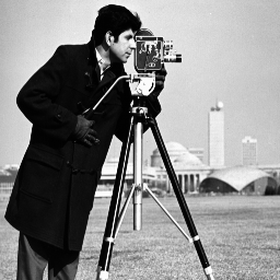
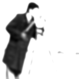
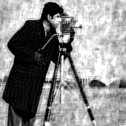
(a)	(b)	(c)

Figure 5: Experiment of Section 5.1: (a) Original image $\overline{x}$. (b) Degraded image $p_{1}$. (c) Recovered image.

5.2 Signal recovery

The goal is to recover the original signal $\overline{x}\in{\mathcal{H}}=C=\mathbb{R}^{N}$ ($N=1024$) shown in Figure 6(a) from the following.

• A piecewise constant approximation $p_{1}$ of $\overline{x}$, given by $p_{1}=\text{\rm proj}_{D_{1}}(\overline{x}+w_{1})$, where $w_{1}\in{\mathcal{G}}_{1}$ represents noise and $D_{1}$ is the subspace of signals in ${\mathcal{G}}_{1}={\mathcal{H}}$ which are constant by blocks along each of the $16$ sets of $64$ consecutive indices in $\{1,\ldots,N\}$ (see Figure 6(b)). The signal-to-noise ratio is $20\log_{10}(\|\overline{x}\|/\|w_{1}\|)=-2.3$ dB. We model this observation by setting $L_{1}=\text{\rm Id}$ and $F_{1}=\text{\rm proj}_{D_{1}}$.

• A bound $\rho_{2}=0.025$ on the magnitude of the finite differences of $\overline{x}$. To enforce this information, following Example 1.2, we set ${\mathcal{G}}_{2}=\mathbb{R}^{N-1}$, $L_{2}\colon{\mathcal{H}}\to{\mathcal{G}}_{2}\colon(\xi_{i})_{1\leqslant i\leqslant N}\mapsto(\xi_{i+1}-\xi_{i})_{1\leqslant i\leqslant N-1}$, $p_{2}=0$, and $F_{2}=\text{\rm Id}-\text{\rm proj}_{D_{2}}$, where $D_{2}=\big{\{}{y\in{\mathcal{G}}_{2}}~{}|~{}{\|y\|_{\infty}\leqslant\rho_{2}}\big{\}}$, that is, using (3.13),

  $$F_{2}\colon(\eta_{k})_{1\leqslant k\leqslant N-1}\mapsto\big{(}{\>\text{\rm soft}}_{{\gamma}}\,(\eta_{k})\big{)}_{1\leqslant k\leqslant N-1}.$$ (5.3)

• A collection of $m=1200$ noisy thresholded scalar observations $r_{3}=(\chi_{j})_{j\in J}\in\mathbb{R}^{m}$ of $\overline{x}$, where $J=\{3,\ldots,m+2\}$. The true data formation model is

  $$(\forall j\in J)\quad\chi_{j}=R({\langle{{\overline{x}}\mid{e_{j}}}\rangle})+\nu_{j},$$ (5.4)

  where $(e_{j})_{j\in J}$ is a dictionary of random vectors in $\mathbb{R}^{N}$ with zero-mean i.i.d. entries, the noise vector $w_{3}=(\nu_{j})_{j\in J}$ yields a signal-to-noise ratio of $20\log_{10}(\|r_{3}\|/\|w_{3}\|)=17.8$ dB, and $R$ is the thresholding operator of the type found in [2, 52] ($\rho=0.05$), namely

  $$R\colon\mathbb{R}\to\mathbb{R}\colon\eta\mapsto\begin{cases}\,\text{\rm sign}(\eta)\sqrt[4]{\eta^{4}-\rho^{4}},&\text{if}\;\;|\eta|>\rho;\\ 0,&\text{if}\;\;|\eta|\leqslant\rho.\end{cases}$$ (5.5)

  We assume that $R$ is misspecified and that the presence of noise is unknown, so that the data acquisition process is incorrectly modeled as

  $$(\forall j\in J)\quad\chi_{j}=Q({\langle{{\overline{x}}\mid{e_{j}}}\rangle}),$$ (5.6)

  where

  $$Q\colon\mathbb{R}\to\mathbb{R}\colon\eta\mapsto\begin{cases}\,\text{\rm sign}(\eta)\sqrt{\eta^{2}-\rho^{2}},&\text{if}\;\;|\eta|>\rho;\\ 0,&\text{if}\;\;|\eta|\leqslant\rho.\end{cases}$$ (5.7)

  Note that $Q$ is not Lipschitzian. Nonetheless, with

  $$S\colon\mathbb{R}\to\mathbb{R}\colon\eta\mapsto\,\text{\rm sign}(\eta)\left(\sqrt{\eta^{2}+\rho^{2}}-\rho\right),$$ (5.8)

  it is straightforward to verify that $S\circ Q={\>\text{\rm soft}}_{{\rho}}\,$ and that, for every $j\in J$, $(F_{j},p_{j})=({\>\text{\rm soft}}_{{\rho}}\,,S\chi_{j})$ is a proxification of $(Q,\chi_{j})$. Also, for every $j\in J$, set ${\mathcal{G}}_{j}=\mathbb{R}$ and $L_{j}={\langle{{\cdot}\mid{e_{j}}}\rangle}$.

We thus obtain an instantiation of Problem 1.3 with $I=\{1,2\}\cup J$ and, for every $i\in I$, $\omega_{i}=1/(\text{\rm card}\,\,I)$. Since $(e_{j})_{j\in J}$ is overcomplete and, for every $j\in J$, $F_{j}$ is surjective, it follows that ${\mathcal{H}}=\big{\{}{\sum_{j\in J}\omega_{j}\eta_{j}e_{j}}~{}|~{}{\eta_{j}\in\text{\rm ran}\,F_{j}}\big{\}}=\sum_{j\in J}\omega_{j}L_{j}^{*}(\text{\rm ran}\,F_{j})\subset\sum_{i\in I}\omega_{i}L_{i}^{*}(\text{\rm ran}\,F_{i})$, so Problem 1.3 is guaranteed to possess a solution by Proposition 4.3(iii). Algorithm (4.15) produces the signal shown in Figure 6(c) with $\gamma=1.9$ and the following activation strategy. At every iteration, $F_{1}$ and $F_{2}$ are activated, while we partition $J$ into four blocks of $300$ elements and cyclically activate one block per iteration, i.e.,

$$(\forall n\in\mathbb{N})(\forall j\in\{0,1,2,3\})\quad I_{4n+j}=\{1,2,3+300j,\ldots,2+300(j+1)\},$$ (5.9)

which satisfies condition (4.14) with $K=4$. This shows that, even when the data is noisy and poorly modeled, Problem 1.3 produces quite robust recoveries. The execution time savings resulting from the use of (5.9) compared to the full activation strategy (i.e., $I_{n}=I$ for every $n\in\mathbb{N}$) are displayed in Figure 7. Note that in very large-scale scenarios in which all data cannot be simultaneously loaded into memory, activation strategies such as (5.9) make algorithm (4.15) implementable.

(a)

(b)

(c)

Figure 6: Experiment of Section 5.2: (a): Original signal $\overline{x}$. (b): Piecewise constant approximation $p_{1}$. (c): Recovered signal.

Figure 7: Experiment of Section 5.2: Relative error $20\log_{10}(\|x_{n}-x_{\infty}\|/\|x_{0}-x_{\infty}\|)$ (dB) versus execution time (seconds) for full activation (red) and cyclic activation (5.9) (green).

5.3 Sparse image recovery

The goal is to recover the original image $\overline{x}\in{\mathcal{H}}=\mathbb{R}^{N}$ ($N=256^{2}$) shown in Figure 8(a) from the following.

• Bounds on pixel values: $x\in C=[0,255]^{N}$.

• The low rank approximation $q_{1}\in{\mathcal{G}}_{1}={\mathcal{H}}$ displayed in Figure 8(b) of a blurred noisy version of $\overline{x}$ modeled as follows. The blurring operator $L_{1}\colon{\mathcal{H}}\to{\mathcal{G}}_{1}$ applies a discrete convolution with a uniform $7\times 7$ kernel, and the operators $Q$ and $S$ are as in Example 3.13, with threshold $\rho=500$. Then $q_{1}=Q(L_{1}\overline{x}+w_{1})$ is a rank-$85$ compression, where $w_{1}\in{\mathcal{G}}_{1}$ induces a blurred image-to-noise ratio of $20\log_{10}(\|L_{1}\overline{x}\|/\|w_{1}\|)=17.6$ dB. By Example 3.13, we obtain a proxification of $(Q,q_{1})$ with $(F_{1},p_{1})=(S\circ Q,Sq_{1})$.

• $\overline{x}$ is sparse. To promote this property in the solutions to (1.10), following Remark 5.1, we set ${\mathcal{G}}_{2}={\mathcal{H}}$, $L_{2}=\text{\rm Id}$, $p_{2}=0$, $\rho_{2}=1.5$, and $F_{2}=\text{\rm proj}_{B_{\infty}(0;\rho_{2})}$.

We therefore arrive at an instance of Problem 1.3 with $I=\{1,2\}$ and $\omega_{1}=\omega_{2}=1/2$. Since $C$ is bounded, Proposition 4.3(ii) guarantees that a solution exists. Algorithm (4.15) with $\gamma=1$ yields the recovery in Figure 8(c). Even though computing $F_{1}$ requires only one singular value decomposition (not two, as (3.14) may suggest), it is the most numerically expensive operator in this problem. Therefore, we choose to activate $F_{1}$ only every $5$ iterations, i.e.,

$$I_{n}=\begin{cases}I\smallsetminus\{1\},&\text{if}\;\;n\not\equiv 0\mod 5;\\ I,&\text{if}\;\;n\equiv 0\mod 5.\end{cases}$$ (5.10)

Figure 10 displays the time savings resulting from the use of (5.10) compared to full activation (both activation strategies yield visually indistinguishable recoveries). Notice that, while the observation in Figure 8(b) is virtually illegible, many of the words in the recovery of Figure 8(c) can be discerned.

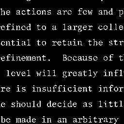
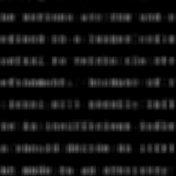
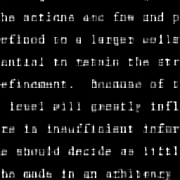
(a)	(b)	(c)

Figure 8: Experiment of Section 5.3: (a) Original image $\overline{x}$. (b) Degraded image $q_{1}$. (c) Recovered image.

Finally, we examine the use of the non firmly nonexpansive sparsity-promoting operator of Example 3.15. Specifically, $Q_{\gamma g}$ is given by (3.16), which is induced by the logarithmic penalty with parameters $\rho=\rho_{2}$ and $\gamma=0.05/\rho_{2}^{2}$. This implies that $0.95Q_{\gamma g}$ is firmly nonexpansive and hence that $\text{\rm Id}-0.95Q_{\gamma g}$ is likewise. Figure 9 displays the result when $F_{2}$ is replaced by componentwise applications of $\text{\rm Id}-0.95Q_{\gamma g}$. In this experiment, the $\ell^{1}$ penalty-based operator $F_{2}$ yields a sharper recovery in Figure 8(c) than the recovery in Figure 9, which is induced by the logarithmic penalty.

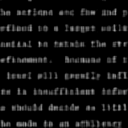
Figure 9: Experiment of Section 5.3: Recovered image with logarithmic thresholding instead of soft thresholding.

Figure 10: Experiment of Section 5.3: Relative error $20\log_{10}(\|x_{n}-x_{\infty}\|/\|x_{0}-x_{\infty}\|)$ (dB) versus execution time (seconds) for full-activation (red) and block activation (5.10) (green).

5.4 Source separation

This experiment incorporates nonlinear compression to a problem in astronomy, which seeks to separate a background image $\overline{x}_{1}\in\mathbb{R}^{N}$ ($N=600^{2}$) of stars from a galaxy image $\overline{x}_{2}\in\mathbb{R}^{N}$ [40]. The goal is to construct the image pair $(\overline{x}_{1},\overline{x}_{2})\in{\mathcal{H}}=\mathbb{R}^{N}\times\mathbb{R}^{N}$ given the following.

• Bounds on pixel values: $(\overline{x}_{1},\overline{x}_{2})\in C=[0,255]^{N}\times[0,255]^{N}$.

• The low rank approximation $q_{1}\in{\mathcal{G}}_{1}=\mathbb{R}^{N}$ shown in Figure 11(b) of the original superposition $\overline{x}_{1}+\overline{x}_{2}$ shown in Figure 11(a), which is modeled as follows. Set $L_{1}\colon{\mathcal{H}}\to{\mathcal{G}}_{1}\colon(x_{1},x_{2})\mapsto x_{1}+x_{2}$, and let $Q$ and $S$ be as in Example 3.13 with $\rho=1500$. The resulting rank-$22$ approximation of $\overline{x}_{1}+\overline{x}_{2}$ is given by $q_{1}=Q(L_{1}(\overline{x}_{1},\overline{x}_{2}))$. It follows from Example 3.13 that $(F_{1},p_{1})=(S\circ Q,Sq_{1})$ is a proxification of $(Q,q_{1})$.

• $\overline{x}_{1}$ is sparse, and $\overline{x}_{2}$ admits a sparse representation relative to the $2$-D discrete cosine transform $L\colon\mathbb{R}^{N}\to\mathbb{R}^{N}$ [40]. To encourage these properties, as discussed in Remark 5.1, we set ${\mathcal{G}}_{2}={\mathcal{H}}$, $L_{2}\colon(x_{1},x_{2})\mapsto(x_{1},Lx_{2})$, $p_{2}=0$, and $F_{2}\colon(y_{1},y_{2})\mapsto(\text{\rm proj}_{B_{\infty}(0;10)}y_{1},\text{\rm proj}_{B_{\infty}(0;45)}y_{2})$. In view of Example 3.1, $F_{2}$ is firmly nonexpansive.

Thus, we arrive at an instance of Problem 1.3 with $I=\{1,2\}$ and $\omega_{1}=\omega_{2}=1/2$. By Proposition 4.3(ii) this problem is guaranteed to possess a solution, since $C$ is bounded. Algorithm (4.15) with $\gamma=1$ provides the solution shown in Figure 11(c)–(d). To improve algorithmic performance, we adopt the activation strategy (5.10); see Figure 12 for time savings compared to the full activation strategy. As can be seen from Figure 11, this approach produces effective recoveries. Even though this problem involves a discontinuous observation process, we can nonetheless solve it with algorithm (4.15), which exploits all of the information at hand.

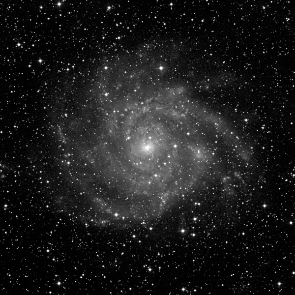
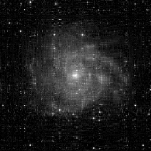
(a)	(b)
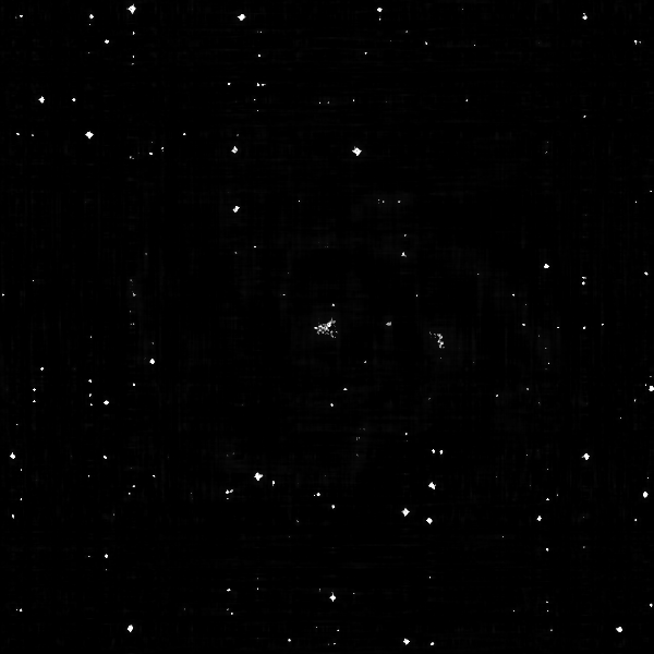
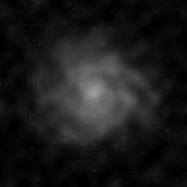
(c)	(d)

Figure 11: Experiment of Section 5.4: (a) Original image $\overline{x}_{1}+\overline{x}_{2}$. (b) Low-rank compression of $\overline{x}_{1}+\overline{x}_{2}$. (c) Recovered background (stars). (d) Recovered foreground (galaxy).

Figure 12: Experiment of Section 5.4: Relative error $20\log_{10}(\|x_{n}-x_{\infty}\|/\|x_{0}-x_{\infty}\|)$ (dB) versus execution time (seconds) for full-activation (red) and block activation (5.10) (green).

References

- [1] J. S. Abel and J. O. Smith, Restoring a clipped signal, Proc. Int. Conf. Acoust. Speech Signal Process., vol. 3, pp. 1745–1748, 1991.
- [2] F. Abramovich, T. Sapatinas, and B. W. Silverman, Wavelet thresholding via a Bayesian approach, J. R. Stat. Soc. Ser. B Stat. Methodol., vol. 60, pp. 725–749, 1998.
- [3] H. Andrews and C. Patterson, Singular value decomposition (SVD) image decoding, IEEE Trans. Commun., vol. 24, pp. 425–432, 1976.
- [4] F. R. Ávila, M. P. Tcheou, and L. W. P. Biscainho, Audio soft declipping based on constrained weighted least squares, IEEE Signal Process. Lett., vol. 24, pp. 1348–1352, 2017.
- [5] R. E. Barlow and H. D. Brunk, The isotonic regression problem and its dual, J. Amer. Stat. Assoc., vol. 67, pp. 140–147, 1972,
- [6] H. H. Bauschke and P. L. Combettes, Convex Analysis and Monotone Operator Theory in Hilbert Spaces, 2nd ed. Springer, New York, 2017.
- [7] I. Bayram and S. Bulek, A penalty function promoting sparsity within and across groups, IEEE Trans. Signal Process., vol. 65, pp. 4238–4251, 2017.
- [8] A. Bensoussan and J.-L. Lions, Applications des Inéquations Variationnelles en Contrôle Stochastique. Bordas, Paris, 1978. English translation: Applications of Variational Inequalities in Stochastic Control. North Holland, New York, 1982.
- [9] H. Boche, M. Guillemard, G. Kutyniok, and F. Philipp, Signal recovery from thresholded frame measurements, Proc. 15th SPIE Wavelets Sparsity Conf., vol. 8858, pp. 80–86, 2013.
- [10] H. Brézis and A. Haraux, Image d’une somme d’opérateurs monotones et applications, Israel J. Math., vol. 23, pp. 165–186, 1976.
- [11] L. M. Briceño-Arias and P. L. Combettes, Convex variational formulation with smooth coupling for multicomponent signal decomposition and recovery, Numer. Math. Theory Methods Appl., vol. 2, pp. 485–508, 2009.
- [12] F. E. Browder, Nonlinear monotone operators and convex sets in Banach spaces, Bull. Amer. Math. Soc., vol. 71, pp. 780–785, 1965.
- [13] J. A. Cadzow, Signal enhancement – A composite property mapping algorithm, IEEE Trans. Acoust., Speech, Signal Process., vol. 36, pp. 49–62, 1988.
- [14] E. Candès and T. Tao, Near-optimal signal recovery from random projections: Universal encoding strategies? IEEE Trans. Inform. Theory, vol. 52, pp. 5406–5425, 2006.
- [15] Y. Censor and T. Elfving, A multiprojection algorithm using Bregman projections in a product space, Numer. Algorithms, vol. 8, pp. 221–239, 1994.
- [16] Y. Censor, T. Elfving, N. Kopf, and T. Bortfeld, The multiple-sets split feasibility problem and its applications for inverse problems, Inverse Problems, vol. 21, pp. 2071–2084, 2005.
- [17] Y. Censor and M. Zaknoon, Algorithms and convergence results of projection methods for inconsistent feasibility problems: A review, Pure Appl. Funct. Anal., vol. 3, pp. 565–586, 2018.
- [18] P. L. Combettes, Inconsistent signal feasibility problems: Least-squares solutions in a product space, IEEE Trans. Signal Process., vol. 42, pp. 2955–2966, 1994.
- [19] P. L. Combettes, The convex feasibility problem in image recovery, in: Advances in Imaging and Electron Physics, (P. Hawkes, ed.), vol. 95, pp. 155–270. Academic Press, New York, 1996.
- [20] P. L. Combettes, Systems of structured monotone inclusions: Duality, algorithms, and applications, SIAM J. Optim., vol. 23, pp. 2420–2447, 2013.
- [21] P. L. Combettes, Monotone operator theory in convex optimization, Math. Program., vol. B170, pp. 177–206, 2018.
- [22] P. L. Combettes and P. Bondon, Hard-constrained inconsistent signal feasibility problems, IEEE Trans. Signal Process., vol. 47, pp. 2460–2468, 1999.
- [23] P. L. Combettes and L. E. Glaudin, Proximal activation of smooth functions in splitting algorithms for convex image recovery, SIAM J. Imaging Sci., vol. 12, pp. 1905–1935, 2019.
- [24] P. L. Combettes and L. E. Glaudin, Solving composite fixed point problems with block updates, Adv. Nonlinear Anal., vol. 10, pp. 1154–1177, 2021.
- [25] P. L. Combettes and J.-C. Pesquet, Deep neural network structures solving variational inequalities, Set-Valued Var. Anal., vol. 28, pp. 491–518, 2020.
- [26] P. L. Combettes and Z. C. Woodstock, A fixed point framework for recovering signals from nonlinear transformations, Proc. Europ. Signal Process. Conf., pp. 2120–2124, 2020.
- [27] P. L. Combettes and Z. C. Woodstock, Reconstruction of functions from prescribed proximal points, 2021. http://arxiv.org/abs/2101.04074
- [28] S. J. Dilworth, N. J. Kalton, D. Kutzarova, and V. N. Temlyakov, The thresholding greedy algorithm, greedy bases, and duality, Constr. Approx., vol. 19, pp. 575–597, 2003.
- [29] M. Ehrgott, Ç. Güler, H. M. Hamacher, and L. Shao, Mathematical optimization in intensity modulated radiation therapy, Ann. Oper. Res., vol. 175, pp. 309–365, 2010.
- [30] F. Facchinei F and J.-S. Pang, Finite-Dimensional Variational Inequalities and Complementarity Problems. Springer, New York, 2003.
- [31] S. Foucart and J. Li, Sparse recovery from inaccurate saturated measurements, Acta Appl. Math., vol. 158, pp. 49–66, 2018.
- [32] M. Goldburg and R. J. Marks II, Signal synthesis in the presence of an inconsistent set of constraints, IEEE Trans. Circuits Syst., vol. 32, pp. 647–663, 1985.
- [33] L. G. Gubin, B. T. Polyak, and E. V. Raik, The method of projections for finding the common point of convex sets, Comput. Math. Math. Phys., vol. 7, pp. 1–24, 1967.
- [34] P. Hall, G. Kerkyacharian, and D. Picard, Block threshold rules for curve estimation using kernel and wavelet methods, Ann. Statist., vol. 26, pp. 922–942, 1998.
- [35] D. Kinderlehrer and G. Stampacchia, An Introduction to Variational Inequalities and Their Applications. Academic Press, New York, 1980.
- [36] L. Knockaert, B. De Backer and D. De Zutter, SVD compression, unitary transforms, and computational complexity, IEEE Trans. Signal Process., vol. 47, pp. 2724–2729, 1999.
- [37] A. M. Legendre, Nouvelles Méthodes pour la Détermination des Orbites des Comètes. Firmin Didot, Paris, 1805.
- [38] D. Malioutov and A. Aravkin, Iterative log thresholding, Proc. Int. Conf. Acoust., Speech, Signal Process., pp. 7198–7202, 2014.
- [39] A. Marmin, A. Jezierska, M. Castella, and J.-C. Pesquet, Global optimization for recovery of clipped signals corrupted with Poisson-Gaussian noise, IEEE Signal Process. Lett., vol. 27, pp. 970–974, 2020.
- [40] M. B. McCoy, V. Cevher, Q. T. Dinh, A. Asaei, and L. Baldassarre, Convexity in source separation: Models, geometry, and algorithms, IEEE Signal Process. Mag., vol. 31, pp. 87–95, 2014.
- [41] K. Nasrollahi and T. B. Moeslund, Super-resolution: A comprehensive survey, Mach. Vis. Appl., vol. 25, pp. 1423–1468, 2014.
- [42] T. Pennanen, On the range of monotone composite mappings, J. Nonlinear Convex Anal., vol. 2, pp. 193–202, 2001.
- [43] B. Peters, B. R. Smithyman, and F. J. Herrmann, Projection methods and applications for seismic nonlinear inverse problems with multiple constraints, Geophys., vol. 84, pp. R251–R269, 2019.
- [44] A. Ranade, S. S. Mahabalarao, and S. Kale, A variation on SVD based image compression, Image Vis. Comput., vol. 25, pp. 771–777, 2007.
- [45] L. Rencker, F. Bach, W. Wang, and M. D. Plumbley, Sparse recovery and dictionary learning from nonlinear compressive measurements, IEEE Trans. Signal Process., vol. 67, pp. 5659–5670, 2019.
- [46] D. Rzepka, M. Miśkowicz, D. Kościelnik, and N. T. Thao, Reconstruction of signals from level-crossing samples using implicit information, IEEE Access, vol. 6, pp. 35001–35011, 2018.
- [47] B. E. A. Saleh, Image synthesis: Discovery instead of recovery, in: H. Stark (ed.) Image Recovery: Theory and Application, pp. 463–498. Academic Press, San Diego, CA, 1987.
- [48] R. J. Samworth, Recent progress in log-concave density estimation, Statist. Sci., vol. 33, pp. 493–509, 2018.
- [49] M. Schetzen, Nonlinear system modeling based on the Wiener theory, Proc. IEEE, vol. 69, pp. 1557–1573, 1981.
- [50] I. Selesnick and M. Farshchian, Sparse signal approximation via nonseparable regularization, IEEE Trans. Signal Process., vol. 65, pp. 2561–2575, 2017.
- [51] N. T. Shaked and J. Rosen, Multiple-viewpoint projection holograms synthesized by spatially incoherent correlation with broadband functions, J. Opt. Soc. Amer. A, vol. 25, pp. 2129–2138, 2008.
- [52] T. Tao and B. Vidakovic, Almost everywhere behavior of general wavelet shrinkage operators, Appl. Comput. Harmon. Anal., vol. 9, pp. 72–82, 2000.
- [53] E. Tarr, Hack Audio. Routledge, New York, 2019.
- [54] V. N. Temlyakov, The best -term approximation and greedy algorithms, Adv. Comput. Math., vol. 8, pp. 249–265, 1998.
- [55] T. Teshima, M. Xu, I. Sato, and M. Sugiyama, Clipped matrix completion: A remedy for ceiling effects, Proc. AAAI Conf. Artif. Intell., pp. 5151–5158, 2019.
- [56] N. T. Thao and M. Vetterli, Deterministic analysis of oversampled A/D conversion and decoding improvement based on consistent estimates, IEEE Trans. Signal Process., vol. 42, pp. 519–531, 1994.
- [57] R. Tibshirani, Regression shrinkage and selection via the lasso: A retrospective, J. R. Statist. Soc. B, vol. 73, pp. 273–282, 2011.
- [58] L. B. White, The wide-band ambiguity function and Altes’ -distribution: Constrained synthesis and time-scale filtering, IEEE Trans. Inform. Theory, vol. 38, pp. 886–892, 1992.
- [59] J.-F. Yang and C.-L. Lu, Combined techniques of singular value decomposition and vector quantization for image coding, IEEE Trans. Image Process., vol. 4, pp. 1141–1146, 1995.
- [60] D. C. Youla, Generalized image restoration by the method of alternating orthogonal projections, IEEE Trans. Circuits Syst., vol. 25, pp. 694–702, 1978.
- [61] D. C. Youla and V. Velasco, Extensions of a result on the synthesis of signals in the presence of inconsistent constraints, IEEE Trans. Circuits Syst., vol. 33, pp. 465–468, 1986.
- [62] D. C. Youla and H. Webb, Image restoration by the method of convex projections: Part 1 – theory, IEEE Trans. Med. Imaging, vol. 1, pp. 81–94, 1982.
- [63] M. Yuan and Y. Lin, Model selection and estimation in regression with grouped variables, J. R. Stat. Soc. Ser. B Stat. Methodol., vol. 68, pp. 49–67, 2006.
- [64] C. A. Zarzer, On Tikhonov regularization with non-convex sparsity constraints, Inverse Problems, vol. 15, art. 025006, 2009.
- [65] E. Zeidler, Nonlinear Functional Analysis and Its Applications II/B: Nonlinear Monotone Operators. Springer, New York, 1990.