Time-dependent conformal transformations
and the propagator for
quadratic systems

Abstract

The method proposed by Inomata and his collaborators allows us to transform a damped Caldiroli-Kanai oscillator with time-dependent frequency to one with constant frequency and no friction by redefining the time variable, obtained by solving a Ermakov-Milne-Pinney equation. Their mapping “Eisenhart-Duval” lifts as a conformal transformation between two appropriate Bargmann spaces. The quantum propagator is calculated also by bringing the quadratic system to free form by another time-dependent Bargmann-conformal transformation which generalizes the one introduced before by Niederer and is related to the mapping proposed by Arnold. Our approach allows us to extend the Maslov phase correction to arbitrary time-dependent frequency. The method is illustrated by the Mathieu profile.
Symmetry 2021 13, 1866. https://doi.org/10.3390/sym13101866

I Introduction

Let us consider a non-relativistic quantum particle with unit mass in $d+1$ space-time dimensions with coordinates $x,t$, given by the natural Lagrangian $L=\hbox{$\textstyle\frac{1}{2}$}{\dot{x}}^{2}-V(x,t)$. The wave function is expressed in terms of the propagator,

$$\psi(x^{\prime\prime},t^{\prime\prime})=\int K(x^{\prime\prime},t^{\prime\prime}|x^{\prime},t^{\prime})\psi(x^{\prime},t^{\prime})dx^{\prime}$$ (I.1)

which, following Feynman’s intuitive proposal FeynmanHibbs , is obtained as,

$$K(x^{\prime\prime},t^{\prime\prime}|x^{\prime},t^{\prime})=\int\exp\big{[}\frac{i}{\hbar}{\cal A}(\gamma)\big{]}{\cal D\gamma}\,,$$ (I.2)

where the (symbolic) integration is over all paths $\gamma(t)=\big{(}x(t),t\big{)}$ which link the space-time point $(x^{\prime},t^{\prime})$ to $(x^{\prime\prime},t^{\prime\prime})$, and where

$${\cal A}(\gamma)=\int_{t^{\prime}}^{t^{\prime\prime}}\!\!\!L\big{(}\gamma(t),\dot{\gamma}(t),t\big{)}dt$$ (I.3)

is the classical action calculated along $\gamma(t)$ FeynmanHibbs ; Schulman ; KLBbook .

The rigourous definition and calculation of (I.2) is beyond our scope here. However the semiclassical approximation leads to the van Vleck-Pauli formula Schulman ; KLBbook ; semiclassic ,

$$K(x^{\prime\prime},t^{\prime\prime}|x^{\prime},t^{\prime})=\left[\frac{i}{2\pi\hbar}\frac{{\partial}^{2}\bar{{\cal A}}}{{\partial}x^{\prime}{\partial}x^{\prime\prime}}\right]^{1/2}\!\exp\left[\frac{i}{\hbar}\bar{{\cal A}}(x^{\prime\prime},t^{\prime\prime}|x^{\prime},t^{\prime})\right]\,,$$ (I.4)

where $\bar{{\cal A}}(x^{\prime\prime},t^{\prime\prime}|x^{\prime},t^{\prime})\!=\!\displaystyle\int_{t^{\prime}}^{t^{\prime\prime}}\!\!\!L(\bar{\gamma}(t),\dot{\bar{\gamma}}(t),t)dt$ is the classical action calculated along the (supposedly unique) classical path $\bar{\gamma}(\tau)$ from $(x^{\prime},t^{\prime})$ and $(x^{\prime\prime},t^{\prime\prime})$. This expression involves data of the classical motion only. We note here also the van Vleck determinant $\frac{{\partial}^{2}\bar{{\cal A}}}{{\partial}x^{\prime}{\partial}x^{\prime\prime}}\,$ in the prefactor semiclassic .

Eqn. (I.4) is exact for a quadratic-in-the-position potentials in $1+1$ dimension $V(x,t)=\hbox{$\textstyle\frac{1}{2}$}\omega^{2}(t)\,x^{2}$ that we consider henceforth.

For $\omega\equiv 0$, i.e., for a free non-relativistic particle of unit mass in 1+1 dimensions with coordinates $X$ and $T$, the result is FeynmanHibbs ; Schulman ; KLBbook ,

$$K_{free}(X^{\prime\prime},T^{\prime\prime}|X^{\prime},T^{\prime})=\left[\frac{1}{2\pi{i}\hbar(T^{\prime\prime}-T^{\prime})}\right]^{1/2}\!\!\exp\left\{\frac{i}{\hbar}\frac{(X^{\prime\prime}-X^{\prime})^{2}}{2(T^{\prime\prime}-T^{\prime})}\right\}\,.$$ (I.5)

An harmonic oscillator with dissipation is in turn described by the Caldirola-Kanai (CK) Lagrangian and equation of motion, respectively Caldirola . For constant damping and harmonic frequency we have,

$$L_{CK}=\frac{1}{2}e^{\lambda_{0}{t}}\Big{(}\big{(}\frac{dx}{dt}\big{)}^{2}-\omega_{0}^{2}x^{2}\Big{)}\,,$$ (I.6a)

$$\frac{d^{2}x}{dt^{2}}+\lambda_{0}\frac{dx}{dt}+\omega_{0}^{2}\,x=0\,$$ (I.6b)

with $\lambda_{0}=\mathop{\rm const.}\nolimits>0$ and $\omega_{0}=\mathop{\rm const.}\nolimits$. A lengthy calculation then yields the exact propagator Schulman ; KLBbook ; Dekker ; Khandekar ; Um02

$$K_{CK}(x^{\prime\prime},t^{\prime\prime}|x^{\prime},t^{\prime})=\left[\frac{\Omega_{0}\,e^{\frac{\lambda_{0}}{2}(t^{\prime\prime}+t^{\prime})}}{2\pi i\hbar\,\sin\big{[}\Omega_{0}(t^{\prime\prime}-t^{\prime})\big{]}}\right]^{\frac{1}{2}}\quad\times$$ (I.7a)

$$\qquad\exp\left\{\frac{i{\Omega_{0}}}{2\hbar\,\sin\big{[}{\Omega_{0}}(t^{\prime\prime}-t^{\prime})\big{]}}\left[(x^{\prime\prime 2}e^{\lambda_{0}t^{\prime\prime}}+x^{\prime 2}e^{\lambda_{0}t^{\prime}})\cos\big{[}{\Omega_{0}}(t^{\prime\prime}-t^{\prime})\big{]}-2x^{\prime\prime}x^{\prime}e^{\lambda_{0}\frac{t^{\prime\prime}+t^{\prime}}{2}}\right]\right\},$$

$${\Omega}_{0}^{2}=\omega_{0}^{2}-\hbox{$\textstyle\frac{1}{4}$}\lambda_{0}^{2}\,,$$ (I.7b)

where an irrelevant phase factor was dropped.

Inomata and his collaborators JunkerInomata ; Cai82 ; Cai generalized (I.7) to time-dependent frequency by redefining time, $t\to\tau$, which allowed them to transform the time-dependent problem to one with constant frequency (see sec.II). Then they follow by what they call a “time-dependent conformal transformation” $(x,t)\to(X,T)$ such that

$$x=f(T)\,X(T)\exp\left[\hbox{$\textstyle\frac{1}{2}$}\lambda_{0}T\right],\;\;\;t=\,g(T)\,,{\quad\text{where}\quad}f^{2}(T)=\,\frac{dg}{dT}\,,$$ (I.8)

which allows them to derive the propagator from the free expression (I.5). When spelled out, (I.8) boils down to a generalized version, (II.11), of the correspondence found by Niederer Niederer73 .

It is legitimate to wonder : in what sense are these transformations “conformal” ? In sec.III we explain that in fact both mappings can be interpreted in the Eisenhart-Duval (E-D) framework as conformal transformations between two appropriate Bargmann spaces Eisenhart ; DBKP ; BurdetOsci ; DGH91 ; dissip . Moreover, the change of variables $x,t\to X,T$ is a special case of the one put forward by Arnold Arnold , and will be shown to be convenient to study explicitly time-dependent systems.

A bonus is the extension to arbitrary time-dependent frequency $\omega(t)$ of the Maslov phase correction Maslov ; Arnold67 ; SMaslov ; Burdet78 ; Schulman ; semiclassic ; HFeynman ; BurdetOsci ; RezendeJMP even when no explicit solutions are available (see sec.IV).

In sec.V.2 we illustrate our theory by the time-dependent Mathieu profile $\omega^{2}(t)=a-2q\cos 2t\,,\,a,b\mathop{\rm const.}\nolimits$ whose direct analytic treatment is complicated.

II The Junker-Inomata derivation of the propagator

Starting with a general quadratic Lagrangian in 1+1 spacetime dimensions with coordinates $\tilde{x}$ and $t$, Junker and Inomata derive the equation of motion JunkerInomata

$$\ddot{\tilde{x}}+\dot{\lambda}(t)\dot{\tilde{x}}+\omega^{2}(t)\tilde{x}=F(t)\,,$$ (II.1)

which describes a non-relativistic particle of unit mass with dissipation $\lambda(t)$. The driving force $F(t)$ can be eliminated by subtracting a particular solution $h(t)$ of (II.1), $x(t)=\tilde{x}(t)-h(t),$ in terms of which (II.1) becomes homogeneous,

$$\ddot{x}+\dot{\lambda}(t)\dot{x}+\omega^{2}(t)x=0\,.$$ (II.2)

This equation can be obtained from the time-dependent generalization of (I.6a),

$$L_{CK}=\frac{1}{2}e^{\lambda(t)}[\dot{x}^{2}-\omega^{2}(t)x^{2}]\,.$$ (II.3)

The friction can be eliminated by setting $x(t)=y(t)\,e^{-\lambda(t)/2}$ which yields an harmonic oscillator with no friction but with shifted frequency Aldaya ,

$$\ddot{y}+\Omega^{2}(t)y=0\;{\quad\text{where}\quad}\;\Omega^{2}(t)=\omega^{2}(t)-\frac{\dot{\lambda}^{2}(t)}{4}-\frac{\ddot{\lambda}(t)}{2}\,.$$ (II.4)

For $\lambda(t)=\lambda_{0}t$ and $\omega=\omega_{0}=\mathop{\rm const.}\nolimits$, for example, we get a usual harmonic oscillator with constant shifted frequency, $\Omega^{2}=\omega_{0}^{2}-{\lambda_{0}^{2}}/{4}=\mathop{\rm const.}\nolimits$

The frequency is in general time-dependent, though, $\Omega=\Omega(t)$, therefore (II.4) is a Sturm-Liouville equation that can be solved analytically only in exceptional cases.

Junker and Inomata JunkerInomata follow another, more subtle path. Eqn. (II.2) is a linear equation with time-dependent coefficients whose solution can be searched for within the Ansatz

$$\;\;\displaystyle{x(t)=\rho(t)\Big{(}Ae^{i{\bar{\omega}}\tau(t)}+Be^{-i{\bar{\omega}}\tau(t)}\Big{)}\,,}\;\;$$ (II.5)

where $A$, $B$ and ${\bar{\omega}}$ are constants and $\rho(t)$ and $\tau(t)$ functions to be found. Inserting (II.5) into (II.2), putting the coefficients of the exponentials to zero, separating real and imaginary parts and absorbing a new integration constant into $A,\,B$ provides us with the coupled system for $\rho(t)$ and $\tau(t)$,

$$\ddot{\rho}+\dot{\lambda}\dot{\rho}+(\omega^{2}(t)-{\bar{\omega}}^{2}\dot{\tau}^{2})\rho=0,$$ (II.6a)

$$\dot{\tau}(t)\,\rho^{2}(t)\,e^{\lambda(t)}=1\,.$$ (II.6b)

Manifestly $\dot{\tau}>0$. Inserting ${\dot{\tau}}$ into (II.6a) then yields the Ermakov-Milne-Pinney (EMP) equation EMP with time-dependent coefficients,

$$\ddot{\rho}+\dot{\lambda}\dot{\rho}+\omega^{2}(t)\rho=\frac{e^{-2\lambda(t)}\bar{\omega}^{2}}{\rho^{3}}\,.$$ (II.7)

We note for later use that eliminating $\rho$ would yield instead

$$\bar{\omega}^{2}=\frac{1}{\dot{\tau}^{2}}\left(\omega^{2}(t)-\frac{1}{2}\frac{\dddot{\tau}}{\dot{\tau}}+\frac{3}{4}\left(\frac{\ddot{\tau}}{\dot{\tau}}\right)^{2}-\frac{\ddot{\lambda}}{2}-\frac{\dot{\lambda}^{2}}{4}\right)\,.$$ (II.8)

Conversely, the constancy of the r.h.s. here can be verified using the eqns (II.6). Equivalently, starting with the Junker-Inomata condition (I.8),

$$\omega^{2}(t)=\frac{\ddot{f}}{f}-2\frac{\dot{f}^{2}}{f^{2}}+\frac{\dot{\lambda}^{2}}{4}+\frac{\ddot{\lambda}}{2}\,.$$ (II.9)

To sum up, the strategy we follow is JunkerInomata ; Galajinsky  :

1. to solve first the EMP equation (II.7) for $\rho$,

2. to integrate (II.6b),

   $$\tau(t)=\int^{t}\!\frac{e^{-\lambda(u)}}{\rho^{2}(u)}\,du\,.$$ (II.10)

Then the trajectory is given by (II.5).

Junker and Inomata show, moreover, that substituting into (II.3) the new coordinates

$$\;\;\displaystyle{T=\frac{\tan{[{\bar{\omega}}\,\tau(t)]}}{{\bar{\omega}}}\,,\qquad X=x\,e^{\frac{\lambda(t)}{2}}\dot{\tau}(t)^{\frac{1}{2}}\sec{[{\bar{\omega}}\,\tau(t)]},}\;\;$$ (II.11)

allows us to present the Caldirola-Kanai action as ,

$${\cal A}_{CK}=\displaystyle\int_{t^{\prime}}^{t^{\prime\prime}}\!\!L_{CK}dt=\int_{T^{\prime}}^{T^{\prime\prime}}\!\frac{1}{2}\big{(}\frac{dX}{dT}\big{)}^{2}dT\,,$$ (II.12)

where we recognize the action of a free particle of unit mass. One checks also directly that $X,T$ satisfy the free equation as they should. The conditions (I.8) are readily verified.

The coordinates $X$ and $T$ describe a free particle, therefore the propagator is (I.5) (as anticipated by our notation). The clue of Junker and Inomata JunkerInomata is that, conversely, trading $X$ and $T$ in (I.5) for $x$ and $t$ allows to derive the propagator for the CK oscillator (see also Um02 , sec.5.1), ,

$$K_{osc}(x^{\prime\prime},t^{\prime\prime}|x^{\prime},t^{\prime})=\left[\frac{{\bar{\omega}}e^{\frac{\lambda^{\prime\prime}+\lambda^{\prime}}{2}}(\dot{\tau}^{\prime\prime}\dot{\tau}^{\prime})^{\frac{1}{2}}}{2\pi i\hbar\,\sin[{\bar{\omega}}(\tau^{\prime\prime}-\tau^{\prime})]}\right]^{\frac{1}{2}}\;\times$$ (II.13)

$$\quad\exp\left\{\frac{i{\bar{\omega}}}{2\hbar\,\sin[{\bar{\omega}}(\tau^{\prime\prime}-\tau^{\prime})]}\left[(x^{\prime\prime 2}e^{\lambda^{\prime\prime}}\dot{\tau}^{\prime\prime}+x^{\prime 2}e^{\lambda^{\prime}}\dot{\tau}^{\prime})\cos[{\bar{\omega}}(\tau^{\prime\prime}-\tau^{\prime})]-2x^{\prime\prime}x^{\prime}e^{\frac{\lambda^{\prime\prime}+\lambda^{\prime}}{2}}(\dot{\tau}^{\prime\prime}\dot{\tau}^{\prime})^{\frac{1}{2}}\right]\right\},\quad$$

where we used the shorthands $\lambda^{\prime\prime}=\lambda(t^{\prime\prime}),\,\tau^{\prime\prime}=\tau(t^{\prime\prime})$, etc.

This remarkable formula says that in terms of “redefined time”, $\tau$, the problem is essentially one with constant frequency. Eqn. (II.13) is still implicit, though, as it requires to solve first the coupled system (II.6) that we can do only in particular cases.

• When $\lambda(t)=\lambda_{0}t$ where $\lambda_{0}=\mathop{\rm const.}\nolimits\geq 0$ eqn (II.2) describes a time-dependent oscillator with constant friction,

  $$\ddot{x}+\lambda_{0}\,\dot{x}+\omega^{2}(t)x=0.$$ (II.14)

  Then setting $R(t)=\rho(t)\,e^{\lambda_{0}t/2}$ eqns (II.6) provide us with the EMP equation for $R$, cf. (II.7),

  $$\ddot{R}+\Omega^{2}(t)R-\frac{\bar{\omega}^{2}}{R^{3}}=0,{\quad\text{where}\quad}\Omega^{2}(t)=\omega^{2}(t)-\frac{\lambda_{0}^{2}}{4}\,.$$ (II.15)

• If, in addition, the frequency is constant $\omega(t)=\omega_{0}=\mathop{\rm const.}\nolimits,$ then eqn (II.15) is solved algebraically by

  $$\bar{\omega}^{2}=\omega_{0}^{2}-\lambda_{0}^{2}/4,\quad R=1{\quad\Rightarrow\quad}\rho(t)=e^{-\lambda_{0}t/2},\quad\tau(t)=t.$$ (II.16)

  Thus $x(t)$ is a linear combination of $e^{-\hbox{$\textstyle\frac{1}{2}$}\lambda_{0}t}\sin\bar{\omega}t$ and $e^{-\hbox{$\textstyle\frac{1}{2}$}\lambda_{0}t}\cos\bar{\omega}t.$ The space-time coordinate transformation of $(x,t)\to(X,T)$ in (II.11) simplifies to the friction-generalized form of that of Niederer Niederer73 ,

  $$T=\frac{\tan(\bar{\omega}{t})}{\bar{\omega}}\,,\quad X=x\exp\left(\frac{1}{2}\lambda_{0}t\right)\sec(\bar{\omega}{t}),$$ (II.17)

  for which the general expression (II.13) reduces to (I.7) when $\lambda_{0}=0$.

• When the oscillator is turned off, $\omega_{0}=0$ but $\lambda_{0}>0$, we have motion in a dissipative medium. The coordinate transformation propagator (II.11) and (II.13) become

  $$X=\frac{2x}{1+\exp\left(-\lambda_{0}t\right)}\,,\qquad T=\frac{2}{\lambda_{0}}\frac{1-\exp(-\lambda_{0}t)}{1+\exp(-\lambda_{0}t)}\,$$ (II.18)

  and

  $$\begin{array}[]{lll}K_{diss}(x^{\prime\prime},t^{\prime\prime}|x^{\prime},t^{\prime})&=&\left[\displaystyle\frac{\lambda_{0}}{2\pi i\hbar[\exp(-\lambda_{0}t^{\prime})-\exp(-\lambda_{0}t^{\prime\prime})]}\right]^{\frac{1}{2}}\\[14.0pt] &&\times\exp\left\{\displaystyle\frac{i\lambda_{0}}{2\hbar}\frac{(x^{\prime\prime}-x^{\prime})^{2}}{\exp(-\lambda_{0}t^{\prime})-\exp(-\lambda_{0}t^{\prime\prime})}\right\}\,,\end{array}$$ (II.19)

  respectively. A driving force $F_{0}$ (e.g. terrestrial gravitation) could be added and then removed by $x\to x+({F_{0}}/{\lambda_{0}})t$.

Further examples can be found in Cai82 ; Cai . An explicitly time-dependent example will be presented in sec. V.2.

III The Eisenhart-Duval lift

Further insight can be gained by “Eisenhart-Duval (E-D) lifting” the system to one higher dimension to what is called a “Bargmann space” Eisenhart ; DBKP ; BurdetOsci ; DGH91 ; dissip . The latter is a $d+1+1$ dimensional manifold endowed with a Lorentz metric whose general form is

$$g_{\mu\nu}dx^{\mu}dx^{\nu}=g_{ij}(x,t)dx^{i}dx^{j}+2dtds-2V(x,t)dt^{2}\,,$$ (III.1)

which carries a covariantly constant null Killing vector ${\partial}_{s}$. Then :

Theorem 1 DBKP ; DGH91  : Factoring out the foliation generated by ${\partial}_{s}$ yields a non-relativistic space-time in $d+1$ dimensions. Moreover, the null geodesics of the Bargmann metric $g_{\mu\nu}$ project to ordinary space-time consistently with Newton’s equations. Conversely, if $(\gamma(t),t)$ is a solution of the non-relativistic equations of motion, then its null lifts to Bargmann space are

$$\big{(}\gamma(t),t,s(t)\big{)},\quad s(t)=s_{0}-{\cal A}(\gamma)=s_{0}-\int^{t}\!\!L(\gamma(r),r)dr$$ (III.2)

where $s_{0}$ is an arbitrary initial value.

Let us consider, for example, a particle of unit mass with the Lagrangian of

$$L=\displaystyle\frac{1}{2\alpha(t)}g_{ij}(x^{k})\dot{x}^{i}\dot{x}^{j}-\beta(t)V(x^{i},t),$$ (III.3)

where $g_{ij}(x^{k})dx^{i}dx^{j}$ is a positive metric on a curved configuration space $Q$ with local coordinates $x^{i}$, $i=1,\ldots,d$. The coefficients $\alpha(t)$ and $\beta(t)$ may depend on time $t$ and $V(x^{i},t)$ is some (possibly time-dependent) scalar potential. The associated equations of motion are

$$\frac{d^{2}x^{i}}{dt^{2}}+\Gamma^{i}_{jk}\frac{dx^{j}}{dt}\frac{dx^{k}}{dt}-\frac{\dot{\alpha}}{\alpha}\frac{dx^{i}}{dt}=-\alpha\beta g^{ij}{\partial}_{j}V\,,$$ (III.4)

where the $\Gamma^{i}_{jk}$ are the Christoffel symbols of the metric $g_{ij}$. For $d=1$, $g_{ij}=\delta_{ij}$ and $V=\hbox{$\textstyle\frac{1}{2}$}\omega^{2}(t)x^{2}$ for $\alpha=\beta=1$ resp. for $\alpha=\beta^{-1}=e^{-\lambda(t)}$ we get a (possible time-dependent) 1d oscillator without resp. with friction, eqn. (I.6), Caldirola ; Dekker ; Aldaya .

Equation (III.4) can also be obtained by projecting a null-geodesic of $d+1+1$ dimensional Bargmann spacetime with coordinates $(x^{\mu})=({x}^{i},t,s)$, whose metric is

$$g_{\mu\nu}dx^{\mu}dx^{\nu}=\frac{1}{\alpha}g_{ij}dx^{i}dx^{j}+2dtds-2\beta Vdt^{2}.$$ (III.5)

For $\alpha=\beta^{-1}=e^{-\lambda(t)}$ we recover (II.2).

Choosing $\lambda(t)=\ln m(t)$ would describe motion with a time-dependent mass $m(t)$. The friction can be removed by the conformal rescaling $x\to y=\sqrt{m}\,x$ and the null geodesics of the rescaled metric describe, consistently with (II.4), an oscillator with no friction but with time-dependent frequency, $\Omega^{2}=\omega^{2}-\frac{\ddot{m}}{2m}+\big{(}\frac{\dot{m}}{2m})^{2}$ Cheng85 .

The friction term $-(\dot{\alpha}/\alpha)\dot{x}^{i}$ in (III.4) can be removed also by introducing a new time-parameter $\tilde{t}$, defined by $d\tilde{t}=\alpha\,dt$ dissip . For $\lambda(t)=\lambda_{0}t$, for example, putting ${\tilde{t}}=-e^{-\lambda_{0}t}/\lambda_{0}$ and eliminates the friction – but it does it at the price of getting manifestly time-dependent frequency Ilderton ; Conf4GW

$$\frac{d^{2}x}{d\tilde{t}^{2}}+\tilde{\Omega}^{2}(\tilde{t})x=0\,,\qquad\tilde{\Omega}^{2}(\tilde{t})=\frac{\omega^{2}}{\tilde{t}^{2}\lambda_{0}^{2}}\,.$$ (III.6)

III.1 The Junker-Inomata Ansatz as a conformal transformation

The approach outlined in sec.II admits a Bargmannian interpretation. For simplicity we only consider the frictionless case $\lambda=0$.

Theorem 2 : The Junker-Inomata method of converting the time-dependent system into one with constant frequency by switching from “real” to “fake time”,

$$t\to\tau(t),\qquad\xi=\sqrt{\dot{\tau}}\,{x}\,$$ (III.7)

induces a conformal transformation between the Bargmann metrics

$$dx^{2}+2dtds-\omega^{2}(t)x^{2}dt^{2} \omega^{2}(t)$$ frequency (III.8a)

$$d\xi^{2}+2d\tau d\sigma-\bar{\omega}^{2}\xi^{2}d\tau^{2}\,, \bar{\omega}=\mathop{\rm const.}\nolimits$$ frequency (III.8b)

$$\;\;\displaystyle{d\xi^{2}+2d\tau d\sigma-\bar{\omega}^{2}\xi^{2}d\tau^{2}=\dot{\tau}(t)\Big{(}dx^{2}+2dtds-\omega^{2}(t)x^{2}dt^{2}\Big{)}\,.}\;\;$$ (III.9)

Proof : Putting $\mu=\ln\dot{\tau}$ allows us to present the constant-frequency $\bar{\omega}$ (II.8) as

$$\bar{\omega}^{2}=\dot{\tau}^{-2}\big{(}\omega^{2}(t)-\hbox{$\textstyle\frac{1}{2}$}\ddot{\mu}+\hbox{$\textstyle\frac{1}{4}$}\dot{\mu}^{2}\big{)}.$$ (III.10)

Then with the notation $\stackrel{{\scriptstyle{\raise 0.5pt\hbox{$\scriptstyle\circ$}}}}{{\xi}}={d\xi}/{d\tau}$ we find,

$$\stackrel{{\scriptstyle{\raise 0.5pt\hbox{$\scriptstyle\circ$}}}}{{\xi}}{}^{2}=\dot{\tau}^{-1}\left[\dot{x}^{2}+\frac{1}{4}\dot{\mu}^{2}x^{2}-\frac{1}{2}\ddot{\mu}x^{2}+\frac{d}{dt}\left(\frac{1}{2}\dot{\mu}x^{2}\right)\right]\,.$$

Let us now recall that the null lift to Bargmann space of a space-time curve is obtained by subtracting the classical action as vertical coordinate,

$$d\sigma=-L(\xi,\stackrel{{\scriptstyle{\raise 0.5pt\hbox{$\scriptstyle\circ$}}}}{{\xi}},\tau)d\tau=-\hbox{$\textstyle\frac{1}{2}$}\big{(}\stackrel{{\scriptstyle{\raise 0.5pt\hbox{$\scriptstyle\circ$}}}}{{\xi}}{}^{2}-\bar{\omega}^{2}\xi^{2}\big{)}d\tau\,.$$ (III.11)

Setting here $\xi={}\dot{\tau}^{1/2}\,x$ and dropping surface terms yields, using the same procedure for the time-dependent-frequency case,

$$d\sigma=ds=-\hbox{$\textstyle\frac{1}{2}$}\big{(}\dot{x}^{2}-\omega^{2}(t)x^{2}\big{)}dt$$ (III.12)

up to surface terms. Then inserting all our formulae into (III.8a) and (III.8b) yields (III.9), as stated. In Junker-Inomata language (I.8), $f(t)=\dot{\tau}^{1/2}\sec(\bar{\omega}\tau),\,g(t)=(\bar{\omega})^{-1}\tan(\bar{\omega}\tau)$ .

Our investigation have so far concerned classical aspects. Now we consider what happens quantum mechanically. Restricting our attention at $d=1$ space dimensions as before we posit that the E-D lift $\widetilde{\psi}$ of a wave function $\psi$ be equivariant,

$$\widetilde{\psi}(x,t,s)=e^{\frac{i}{\hbar}s}\psi(x,t){\quad\Rightarrow\quad}{\partial}_{s}\widetilde{\psi}=\frac{i}{\hbar}\widetilde{\psi}\,.$$ (III.13)

Then the massless Klein-Gordon equation for $\widetilde{\psi}$ associated with the $1+1+1=3$ d Barmann- metric implies the Schrödinger equation in 1+1 d,

$$\Delta_{g}\,\widetilde{\psi}=0{\quad\Rightarrow\quad}i{\partial}_{t}\psi=\big{[}-\frac{\hbar^{2}}{2}\Delta_{x}+V(x,t)\big{]}\psi\,$$ (III.14)

where $\Delta_{g}$ is the Laplace-Beltrami operator associated with the metric. In $d=1$ it is of course $\Delta_{x}={\partial}_{x}^{2}$ .

A conformal diffeomorphism $(X,T,S)\to\tilde{f}(X,T,S)=(x,t,s)$ with conformal factor $\sigma^{2}_{f}$, $\tilde{f}^{*}g_{\mu\nu}=\sigma^{2}_{f}{\,}g_{\mu\nu},$ projects to a space-time transformation $(X,T)\to{f}(X,T)=(x,t)$. It is implemented on a wave function lifted to Bargmann space as

$$\widetilde{\psi}(x,t,s)=\sigma_{f}^{-1/2}\widetilde{\psi}(X,T,S)$$ (III.15)

In secs.IV.2 these formulae will be applied to the Niederer map (IV.12).

III.2 The Arnold map

The general damped harmonic oscillator with time-dependent driving force $F(t)$ in 1+1 dimensions, (II.1),

$$\ddot{x}+\dot{\lambda}\dot{x}+\omega^{2}\left(t\right)x=F(t)\,,$$ (III.16)

can be solved by an Arnold transformation Arnold which “straightens the trajectories” Aldaya ; LopezRuiz ; dissip . To this end one introduces new coordinates,

$$T=\frac{u_{1}}{u_{2}}\,,\quad X=\frac{x-u_{p}}{u_{2}}\,,$$ (III.17)

where $u_{1}$ and $u_{2}$ are solutions of the associated homogeneous equation (III.16) with $F\equiv 0$ and $u_{p}$ is a particular solution of the full equation (III.16). It is worth noting that (III.17) allows to check, independently, the Junker-Inomata criterion in (I.8). The initial conditions are chosen as,

$$u_{1}\left(t_{0}\right)=\dot{u}_{2}\left(t_{0}\right)=0,\ \ \dot{u}_{1}\left(t_{0}\right)=u_{2}\left(t_{0}\right)=1,\ \ u_{p}\left(t_{0}\right)=\dot{u}_{p}\left(t_{0}\right)=0.$$ (III.18)

Then in the new coordinates the motion becomes free Arnold ,

$$X(T)=aT+b\,,\qquad a,b=\mathop{\rm const.}\nolimits$$ (III.19)

Eqn (III.16) can be obtained by projecting a null geodesic of the Bargmann metric

$${g}_{\mu\nu}d{x}^{\mu}d{x}^{\nu}=e^{\lambda(t)}dx^{2}+2dtds-2e^{\lambda(t)}\left(\frac{1}{2}\omega(t)^{2}x^{2}-F(t)x\right)dt^{2}\,.$$ (III.20)

Completing (III.17) by

$$S=s+e^{\lambda}u_{2}^{-1}\left(\frac{1}{2}\dot{u}_{2}x^{2}+\dot{u}_{p}x\right)+g\left(t\right){\quad\text{where}\quad}\dot{g}=\frac{1}{2}e^{\lambda}\left(\dot{u}_{p}^{2}-\omega^{2}u_{p}^{2}+2Fu_{p}\right)\,$$ (III.21)

lifts the Arnold map to Bargmann spaces, $(x,t,s)\to(X,T,S)$ ,

$${g}_{\mu\nu}d{x}^{\mu}d{x}^{\nu}=e^{\lambda(t)}u_{2}^{2}(t)\big{(}dX^{2}+2dTdS\big{)}\,.$$ (III.22)

The oscillator metric (III.20) is thus carried conformally to the free one, generalizing earlier results DBKP ; BurdetOsci ; DHP2 . For the damped harmonic oscillator with $\lambda(t)=\lambda_{0}t$ and $F(t)\equiv 0$, $u_{p}\equiv 0$ is a particular solution. When $\omega=\omega_{0}=\mathop{\rm const.}\nolimits$, for example,

$$u_{1}=e^{-{\lambda_{0}}t/2}\frac{\sin\Omega_{0}t}{\Omega_{0}},\;u_{2}=e^{-{\lambda_{0}}t/2}\big{(}\cos\Omega_{0}t+\frac{\lambda_{0}}{2\Omega_{0}}\sin\Omega_{0}t\big{)}\,,\quad\Omega_{0}^{2}=\omega_{0}^{2}-{\lambda_{0}^{2}}/{4}\;$$ (III.23)

are two independent solutions of the homogeneous equation with initial conditions (III.18) and provide us with

$$T =\frac{\sin\Omega_{0}t}{\Omega_{0}(\cos\Omega_{0}t+\frac{\lambda_{0}}{2\Omega_{0}}\sin\Omega_{0}t)},$$ (III.24a)

$$X =\frac{e^{{\lambda_{0}}t/2}\,x}{\cos\Omega_{0}t+\frac{\lambda_{0}}{2\Omega_{0}}\sin\Omega_{0}t},$$ (III.24b)

$$S =s-{\hbox{$\textstyle\frac{1}{2}$}}e^{{\lambda_{0}}t}x^{2}\,\big{(}\frac{\omega_{0}^{2}}{\Omega_{0}}\big{)}\,\frac{\sin\Omega_{0}t}{\cos\Omega_{0}t+\frac{\lambda_{0}}{2\Omega_{0}}\sin\Omega_{0}t}\,.$$ (III.24c)

In the undamped case $\lambda_{0}=0$ thus $\Omega_{0}=\omega_{0}$, and (III.24) reduces to that of Niederer Niederer73 lifted to Bargmann space BurdetOsci ; DGH91 ,

$$T=\frac{\tan\omega_{0}t}{\omega_{0}},\qquad X=\frac{x}{\cos\omega_{0}t},\qquad S=s-{\hbox{$\textstyle\frac{1}{2}$}}x^{2}\omega_{0}\tan\omega_{0}t.$$ (III.25)

The Junker-Inomata construction in sec.II can be viewed as a particular case of the Arnold transformation. We choose $u_{p}\equiv 0$ and the two independent solutions

$$u_{1}=e^{-\lambda/2}\,\dot{\tau}^{-1/2}\,\frac{\sin\bar{\omega}\tau}{\bar{\omega}},\qquad u_{2}=e^{-\lambda/2}\,\dot{\tau}^{-1/2}\,\cos\bar{\omega}\tau\,.$$ (III.26)

The initial conditions (III.18) at $t_{0}=0$ imply $\tau(0)=\dot{\rho}(0)=0,\,\rho(0)=\dot{\tau}(0)=1.$ Then spelling out (III.21),

$$S=s-\frac{1}{2}e^{\lambda}\left(\bar{\omega}\dot{\tau}\tan\bar{\omega}\tau+\frac{1}{2}\dot{\lambda}+\frac{1}{2}\frac{\ddot{\tau}}{\dot{\tau}}\right)x^{2}$$ (III.27)

completes the lift of (II.11) to Bargmann spaces. In conclusion, the one-dimensional damped harmonic oscillator is described by the conformally flat Bargmann metric,

$$\;\;\displaystyle{{g}_{\mu\nu}d{x}^{\mu}d{x}^{\nu}=\frac{\cos^{2}\bar{\omega}\tau}{\dot{\tau}}\big{(}dX^{2}+2dTdS\big{)}.}\;\;$$ (III.28)

The metric (III.28) is manifestly conformally flat, therefore its geodesics are those of the free metric, $X(T)=aT+b$. Then using (III.17) with (III.26) yields

$$\;\;\displaystyle{x(t)=e^{-\lambda(t)/2}\,\dot{\tau}^{-1/2}(t)\left(a\frac{\sin[\bar{\omega}\tau(t)]}{\bar{\omega}}+b\,\cos[\bar{\omega}\tau(t)]\,\right).}\;\;$$ (III.29)

The bracketed quantity here describes a constant-frequency oscillator with “time” $\tau(t)$. The original position, $x$, gets a time-dependent “conformal” scale factor.

IV The Maslov correction

As mentioned before, the semiclassical formula (I.7) is correct only in the first oscillator half-period, $0<t^{\prime\prime}-t^{\prime}<\pi/\Omega_{0}$. Its extension for all $t$ involves the Maslov correction. In the constant-frequency case with no friction, for example, assuming that $\Omega_{0}(t^{\prime\prime}-t^{\prime\prime})/\pi$ is not an integer, we have Schulman ; KLBbook ; HFeynman ,

$$K^{ext}(x^{\prime\prime},t^{\prime\prime}|x^{\prime},t^{\prime}) = \left[\frac{\Omega_{0}}{2\pi\hbar\,\big{|}\sin\Omega_{0}(t^{\prime\prime}-t^{\prime})\big{|}}\right]^{\frac{1}{2}}\times\,e^{-i\frac{\pi}{4}(1+2\ell)}$$

$$\exp\left\{\frac{i\Omega_{0}}{2\hbar\,\sin\Omega_{0}(t^{\prime\prime}-t^{\prime})}\left[({x^{\prime\prime}}^{2}+{x^{\prime}}^{2})\cos\Omega_{0}(t^{\prime\prime}-t^{\prime})-2x^{\prime\prime}x^{\prime}\right]\right\}\,,\quad$$

where the integer

$$\ell={\rm Ent}\big{[}\frac{\Omega_{0}(t^{\prime\prime}-t^{\prime})}{\pi}\big{]}\,$$ (IV.2)

is called as the Maslov index (where ${\rm Ent}[x]$ is the integer part of $x$). $\ell$ counts the completed half-periods, and is related also to the Morse index which counts the negative modes of ${\partial}^{2}{\cal A}/{\partial}x^{\prime}{\partial}x^{\prime\prime}$ semiclassic .

Now we generalize (IV) to time-dependent frequency :

Theorem 4 : In terms of $\bar{\omega}$ and $\tau$ introduced in sec.II,

• Outside caustics, i.e., for $\bar{\omega}(\tau^{\prime\prime}-\tau^{\prime})\neq\pi\ell$, the propagator for the harmonic oscillator with time-dependent frequency and friction is

  $$\hskip-14.22636ptK^{ext}(x^{\prime\prime},t^{\prime\prime}|x^{\prime},t^{\prime})=\left[\frac{\bar{\omega}e^{\frac{\lambda^{\prime\prime}+\lambda^{\prime}}{2}}(\dot{\tau}^{\prime\prime}\dot{\tau}^{\prime})^{\frac{1}{2}}}{2\pi\hbar|\sin\bar{\omega}(\tau^{\prime\prime}-\tau^{\prime})|}\right]^{1/2}\exp\left\{-\frac{i\pi}{2}\left(\frac{1}{2}+{\rm Ent}\big{[}\frac{\bar{\omega}(\tau^{\prime\prime}-\tau^{\prime})}{\pi}\big{]}\right)\right\}$$ (IV.3)

  $$\times\exp\left\{\frac{i\bar{\omega}}{2\hbar\sin\bar{\omega}(\tau^{\prime\prime}-\tau^{\prime})}[(x^{\prime\prime 2}e^{\lambda^{\prime\prime}}\dot{\tau}^{\prime\prime}+x^{\prime 2}e^{\lambda^{\prime}}\dot{\tau}^{\prime})\cos[\bar{\omega}(\tau^{\prime\prime}-\tau^{\prime})]-2x^{\prime\prime}x^{\prime}e^{\frac{\lambda^{\prime\prime}+\lambda^{\prime}}{2}}(\dot{\tau}^{\prime\prime}\dot{\tau}^{\prime})^{\frac{1}{2}}]\right\}\,\quad\;$$

• At caustics, i.e., for

  $$\;\;\displaystyle{\bar{\omega}(\tau^{\prime\prime}-\tau^{\prime})=\pi\,\ell,\quad\ell=0,\pm 1,\dots\,}\;\;$$ (IV.4)

  we have instead HFeynman ; KLBbook ,

  $$K^{ext}\Big{(}x^{\prime\prime},x^{\prime},|\tau^{\prime\prime}-\tau^{\prime}=\frac{\pi}{\bar{\omega}}\ell\Big{)}=\big{[}e^{\frac{\lambda^{\prime\prime}+\lambda^{\prime}}{2}}(\dot{\tau}^{\prime\prime}\dot{\tau}^{\prime})^{\frac{1}{2}}\big{]}^{1/2}$$ (IV.5)

  $$\qquad\times\exp\left(-\frac{i\pi\ell}{2}\right)\delta\Big{(}x^{\prime}\exp(\lambda^{\prime}/2)\dot{\tau}^{\prime 1/2}-(-1)^{k}x^{\prime\prime}\exp(\lambda^{\prime\prime}/2)\dot{\tau}^{\prime\prime 1/2}\Big{)}\,.$$

Proof : In terms of the redefined coordinates

$$\tau=\tau(t){\quad\text{and}\quad}\xi=x\exp\left[\frac{\lambda(t)}{2}\right]\dot{\tau}^{1/2}(t),$$ (IV.6)

cf. (III.7) and using the notation $\stackrel{{\scriptstyle{\raise 0.5pt\hbox{$\scriptstyle\circ$}}}}{{\{\,\cdot\,\}}}=d/d\tau$, the time-dependent oscillator equation (II.2) is taken into

$$\stackrel{{\scriptstyle{\raise 0.5pt\hbox{$\scriptstyle\circ$}}{\raise 0.5pt\hbox{$\scriptstyle\circ$}}}}{{\xi}}+\,\bar{\omega}^{2}\xi=0\,,{\quad\text{where}\quad}\bar{\omega}^{2}=\frac{1}{\dot{\tau}^{2}}\left(\omega^{2}(t)-\frac{1}{2}\frac{\dddot{\tau}}{\dot{\tau}}+\frac{3}{4}\left(\frac{\ddot{\tau}}{\dot{\tau}}\right)^{2}-\frac{\ddot{\lambda}}{2}-\frac{\dot{\lambda}^{2}}{4}\right)\,.$$ (IV.7)

Thus the problem is reduced to one with time independent frequency, $\bar{\omega}$ in (II.8) .

Let us now recall the formula #(19) of Junker and Inomata in JunkerInomata which tells us how propagators behave under the coordinate transformation $(\xi,\tau)\longleftrightarrow(x,t)$  :

$$K_{2}(x^{\prime\prime},t^{\prime\prime}|x^{\prime},t^{\prime})=\left[\left(\frac{\partial\xi^{\prime}}{\partial x^{\prime}}\right)\left(\frac{\partial\xi^{\prime\prime}}{\partial x^{\prime\prime}}\right)\right]^{\frac{1}{2}}K_{1}(\xi^{\prime\prime},\tau^{\prime\prime}|\xi^{\prime},\tau^{\prime})\,.$$ (IV.9)

Here $K_{2}=K^{ext}$ is the propagator of an oscillator with time-dependent frequency and friction, $\omega(t)$ and $\lambda(t)$, respectively — the one we are trying to find. $K_{1}$ is in turn the Maslov-extended propagator of an oscillator with no friction and constant frequency, as in (IV). Then the propagator for the harmonic oscillator with time-dependent frequency and friction, eqn. (IV.3), is obtained using (IV.6).

Notice that (IV.3) is regular at the points $r_{k}\in J_{k}$ where $\sin=\pm 1$. However at caustics, $\tau^{\prime\prime}-\tau^{\prime}=(\pi/\bar{\omega})\ell$, $K^{ext}$ diverges and we have instead (IV.5).

Henceforth we limit our investigations to $\lambda=0$.

IV.1 Properties of the Niederer map

More insight is gained from the perspective of the generalized Niederer map (II.11). We first study their properties in some detail. For simplicity we choose, in the rest of this section, $x^{\prime}=t^{\prime}=0$ and $x^{\prime\prime}\equiv x$ and $t^{\prime\prime}\equiv t$.

We start with the observation that the Niederer map (II.11) becomes singular where the cosine vanishes, i.e., where

$$\cos[\bar{\omega}\tau(r_{k})]=0,\quad\text{i.e.}\quad\tau(r_{k})=(k+\hbox{$\textstyle\frac{1}{2}$})\frac{\pi}{\bar{\omega}},\quad k=0\,,\pm 1,\dots$$ (IV.10)

$r_{k}<r_{k+1}$ because $\tau(t)$ is an increasing function by (II.10). Moreover, each interval

$$I_{k}=\big{[}r_{k},r_{k+1}\big{]},\quad k=0,\pm 1,\dots\,$$ (IV.11)

is mapped by (II.11) onto the full range $-\infty<T<\infty$. Therefore the inverse mapping is multivalued, labeled by integers $k$,

$$N_{k}~{}:T\to t=\frac{\arctan_{k}\bar{\omega}{T}}{\bar{\omega}}\,,\quad X\to x=\frac{X}{\sqrt{1+\bar{\omega}^{2}T^{2}}}\,,$$ (IV.12)

where $\arctan_{k}(\,\cdot\,)=\arctan_{0}(\,\cdot\,)+k\pi$ with $\arctan_{0}(\,\cdot\,)$ the principal determination i.e. in $(-\pi/2,\pi/2)$.

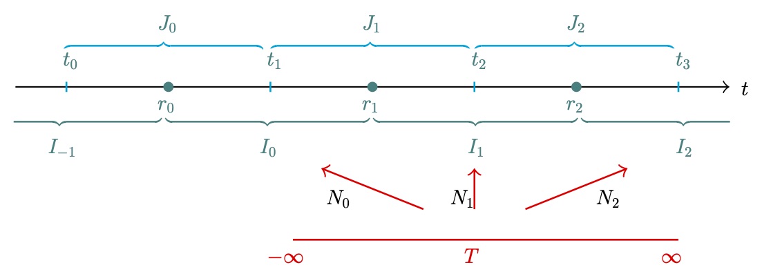
Figure 1: The generelized Niederer map (II.11) maps each interval ${\bf I_{k}=(r_{k},r_{k+1})}$ onto the entire real line $-\infty<T<\infty$. Its inverse mapping is therefore multivalued, labeled by an integer $k$. The classical motions and the propagator are both regular at the separation points ${\bf r_{k}}$. All classical trajectories are focused at the caustic points ${\bf t_{\ell}}$, where the propagator diverges.

Then $\lim_{t\to r_{k}-}\tan{t}=\infty$ and $\lim_{t\to r_{k}+}\tan{t}=-\infty$ imply that

$$\lim_{T\to\infty}{N_{k}}(T)=\;r_{k+1}\;=\lim_{T\to-\infty}N_{k+1}(T)\,.$$ (IV.13)

Therefore the intervals $I_{k}$ and $I_{k+1}$ are joined at $r_{k+1}$ and the $I_{k}$ form a partition the time axis, $\big{\{}-\infty<t<\infty\big{\}}={\cup}_{k}I_{k}\,.$

Returning to (IV.3) (which is (IV) with $\Omega_{0}\Rightarrow\bar{\omega},\,t\Rightarrow\tau$) we then observe that whereas the propagator is regular at $r_{k}$, it diverges at caustics,

$$\sin[\bar{\omega}\tau(t_{\ell})]=0\quad\text{i.e.}\quad\tau(t_{\ell})=\frac{\pi}{\bar{\omega}}\,\ell,\quad{\ell}=0,\,\pm 1,\dots\,,$$ (IV.14)

cf. (IV.4). Thus $t_{\ell}\leq t_{\ell+1}$, and

$$N_{k}(-\infty)=r_{k},\quad N_{k}(T=0)=t_{k+1},\quad N_{k}(+\infty)=r_{k+1}\,.$$ (IV.15)

Thus $N_{k}$ maps the full $T$-line into $I_{k}$ with $t_{k}$ an internal point. Conversely, $r_{k}$ is an internal point of $J_{k}$. The intervals $J_{\ell}=\big{[}t_{\ell},t_{\ell+1}\big{]}$ cover again the time axis, $\displaystyle\cup_{\ell}J_{\ell}=\big{\{}-\infty<t<\infty\big{\}}\,.$

By (III.29) the classical trajectories are regular at $t=r_{k}$. Moreover, for arbitrary initial velocities,

$$\sqrt{\dot{\tau}(t_{\ell+1})}{\,}x(t_{\ell+1})=-\sqrt{\dot{\tau}(t_{\ell})}{\,}x(t_{\ell})\,$$ (IV.16)

implying that after a half-period $\bar{\omega}\tau\to\bar{\omega}\tau+\pi$ all classical motions are focused at the same point. The two entangled sets of intervals are shown in fig.1.

The Niederer map (III.25) “E-D lifts” to Bargmann space.

Theorem 3. The E-D lift of the inverse of the Niederer map (III.25) we shall denote by $\widetilde{N}_{k}:(X,T,S)\to(x,t,s)$ ($t\in I_{k}$) is

$$t=\frac{\arctan_{k}\bar{\omega}T}{\bar{\omega}}\,,\quad x=\frac{X}{\sqrt{1+\bar{\omega}^{2}T^{2}}}\,,\quad s=S+\frac{X^{2}}{2}\frac{\bar{\omega}^{2}T}{1+\bar{\omega}^{2}T^{2}}\,.$$ (IV.17)

Note that $t$ depends on $k$, $t=N_{k}(T)$, but $x$ and $s$ do not.

Proof : These formulæ follow at once by inverting (III.25) at once with the cast $\omega_{0}\Rightarrow\bar{\omega},\,t\Rightarrow\tau$. Alternatively, it could also be proven as for of Theorem 2.

For each integer $k$ (IV.17) maps the real line $-\infty<T<\infty$ into the “open strip” BurdetOsci $\big{[}r_{k},r_{k+1}\big{]}\times{\mathbb{R}}^{2}\equiv I_{k}\times{\mathbb{R}}^{2}$ with $r_{k}$ defined in (IV.10). Their union covers the entire Bargmann manifold of the oscillator.

Now we pull back the free dynamics by the multivalued inverse (IV.17). We put $\bar{\omega}=1$ for simplicity. The free motion with initial condition $X(0)=0$,

$$X(T)=aT,\quad S(T)=S_{0}-\frac{a^{2}}{2}T\,,$$ (IV.18)

E-D lifts by (IV.17) to

$$x(t)=a\sin t\qquad s(t)=S_{0}-\frac{a^{2}}{4}\sin 2t\,,$$ (IV.19)

consistently with $s(t)=s_{0}-\bar{\cal A}_{osc}$, as it can be checked directly. Note that the $s$ coordinate oscillates with doubled frequency.

• At $t=r_{k}=(\hbox{$\textstyle\frac{1}{2}$}+k)\pi$ (where the Niederer maps are joined), we have, $\lim_{t\to r_{k}}x(t)=(-1)^{k+1}a\,,\;\lim_{t\to r_{k}}s(t)=S_{0}.$ Thus the pull-backs of the Bargmann-lifts of free motions are glued to smooth curves.

• Similarly at t caustics $t=t_{\ell}=\pi\ell$ we infer from (IV.19) that for all initial velocity $a$ and for all $\ell$ $\lim_{t\to t_{\ell}}x(t)=0,\,\lim_{t\to t_{\ell}}s(t)=S_{0}\,.$ Thus the lifts are again smooth at $t_{\ell}$ and after each half-period all motions are focused above the initial position $(x(0)=0,s(0)=S_{0})$.

IV.2 The propagator by the Niederer map

Now we turn at the quantum dynamics. Our starting point is the free propagator (I.5) which (as mentioned before) is valid only for $0<T^{\prime\prime}-T^{\prime}$. Its extension to all $T$ involves the sign of $(T^{\prime\prime}-T^{\prime})$ BurdetOsci .

Let us explain this subtle point in some detail. First of all, we notice that the usual expression (I.5) involves a square root which is double-valued, obliging us to choose one of its branches. Which one do we choose is irrelevant – it is a mere gauge choice. However once we do choose one, we must stick to our choice. Take, for example, the one for which $\sqrt{-i}=e^{-i\pi/4}$ — then the prefactor in (I.5) is

$$\left[\frac{1}{2\pi{i}\hbar(T^{\prime\prime}-T^{\prime})}\right]^{1/2}=e^{-i\pi/4}\left[\frac{1}{2\pi\hbar\big{|}T^{\prime\prime}-T^{\prime}\big{|}}\right]^{1/2}.$$

Let us now consider what happens when $T^{\prime\prime}-T^{\prime}$ changes sign. Then the prefactor gets multiplied by $\sqrt{-1}\,$ so it becomes, for the same choice of the square root,

$$e^{i\pi/2\,}e^{-i\pi/4}\left[\frac{1}{2\pi\hbar\big{|}T^{\prime\prime}-T^{\prime}\big{|}}\right]^{1/2}=e^{+i\pi/4}\left[\frac{1}{2\pi\hbar\big{|}T^{\prime\prime}-T^{\prime}\big{|}}\right]^{1/2}.$$ (IV.20)

In conclusion, the formula valid for all $T$ is,

$$K_{free}(X^{\prime\prime},T^{\prime\prime}|X^{\prime},T^{\prime})=e^{-{i}\hbox{$\textstyle\frac{\pi}{4}$}\,{\rm sign}(T^{\prime\prime}-T^{\prime})}\left[\displaystyle\frac{1}{2\pi\hbar|T^{\prime\prime}-T^{\prime}|}\right]^{1/2}\!\!\exp\left\{\displaystyle\frac{i}{\hbar}\bar{\cal A}_{free}\right\}\,,$$ (IV.21)

where

$$\bar{\cal A}_{free}=\frac{(X^{\prime\prime}-X^{\prime})^{2}}{2(T^{\prime\prime}-T^{\prime})}\,$$ (IV.22)

is the free action calculated along the classical trajectory. Let us underline that (IV.21) already involves a “Maslov jump” $e^{-i\pi/2\,}$ – which, for a free particle, happens at $T=0$. For $T^{\prime\prime}-T^{\prime}=0$ we have $K_{free}=\delta(X^{\prime\prime}-X^{\prime})$.

Accordingly, the wave function $\Psi\equiv\Psi_{free}$ of a free particle is, by (I.1),

$$\Psi\left(X^{\prime\prime},T^{\prime\prime}\right)\!=\!e^{-i\frac{\pi}{4}\!\mathrm{sign}\left(T^{\prime\prime}-T^{\prime}\right)}\left[\frac{1}{2\pi\hbar|T^{\prime\prime}-T^{\prime}|}\right]^{1/2}\!\!\int_{{\mathbb{R}}}\exp\left\{\frac{i}{\hbar}\bar{\cal A}_{free}\right\}\Psi\left(X^{\prime},T^{\prime}\right)dX^{\prime}\,.\quad$$ (IV.23)

Now we pull back the free dynamics using the multivalued inverse Niederer map. It is sufficient to consider the constant-frequency case $\bar{\omega}=\mathop{\rm const.}\nolimits$ and denote time by $t$. Let $t$ belong to the range of $N_{k}$ in (IV.12), $t\in I_{k}=[r_{k},r_{k+1}]=N_{k}\big{(}\{-\infty<T<\infty\}\big{)}.$ Then applying the general formulae in sec.III.1 yields BurdetOsci ,

$$\begin{array}[]{lll}\widetilde{\psi}(x^{\prime\prime},t^{\prime\prime},s^{\prime\prime})&=&\cos^{-1/2}[\bar{\omega}(t^{\prime\prime}-t^{\prime})]\widetilde{\Psi}(X^{\prime\prime},T^{\prime\prime},S^{\prime\prime})=e^{-\frac{i\pi}{4}\mathrm{sign}\left(\frac{\tan\bar{\omega}(t^{\prime\prime}-t^{\prime\prime})}{\bar{\omega}}\right)}\times\\[8.0pt] &&\cos^{-1/2}\left[\bar{\omega}(t^{\prime\prime}-t^{\prime})\right]\exp\left(\frac{i}{\hbar}s^{\prime\prime}\right)\exp\left(-\frac{i}{\hbar}(\frac{1}{2}\bar{\omega}{x^{\prime\prime}}^{2}\tan[\bar{\omega}(t^{\prime\prime}-t^{\prime\prime})]\right)\\[8.0pt] &&\quad\sqrt{\displaystyle\frac{|\bar{\omega}|}{2\pi\hbar|\tan[\bar{\omega}(t^{\prime\prime}-t^{\prime})]|}}\displaystyle\int_{{\mathbb{R}}}\!\exp\left\{\frac{i}{\hbar}\frac{{\bar{\omega}}|\frac{{x^{\prime\prime}}}{\cos[\bar{\omega}(t^{\prime\prime}-t^{\prime})]}-x^{\prime}|^{2}}{2\tan[\bar{\omega}(t^{\prime\prime}-t^{\prime})]}\right\}\psi(x^{\prime},t^{\prime})dx^{\prime}\,.\end{array}$$

However the second exponential in the middle line combines with the integrand in the braces in the last line to yield the action calculated along the classical oscillator trajectory,

$$\bar{\cal A}_{osc}=\frac{\bar{\omega}}{2\sin\bar{\omega}(t^{\prime\prime}-t^{\prime})}\big{(}({x^{\prime\prime}}^{2}+{x^{\prime}}^{2})\cos\bar{\omega}(t^{\prime\prime}-t^{\prime})-2x^{\prime\prime}x^{\prime}\big{)}\,.$$ (IV.24)

Thus using the equivariance we end up with,

$$\psi_{osc}\left(x^{\prime\prime},t^{\prime\prime}\right) = \cos^{-1/2}[\bar{\omega}(t^{\prime\prime}-t^{\prime})]\,\exp\left[-\frac{i\pi}{4}\mathrm{sign}\left(\frac{\tan[\bar{\omega}(t^{\prime\prime}-t^{\prime})]}{\bar{\omega}}\right)\right]\times\quad$$

$$\sqrt{\frac{|\bar{\omega}|}{2\pi\hbar|{\tan[\bar{\omega}(t^{\prime\prime}-t^{\prime})]}|}}\int_{{\mathbb{R}}}\exp\left\{\frac{i}{\hbar}\bar{\cal A}_{osc}\right\}\psi_{osc}\left(x^{\prime},t^{\prime}\right)dx\,.$$

Now we recover the Maslov jump which comes from the first line here. For simplicity we consider again $t^{\prime}=0,\,x^{\prime}=0$ and denote $t^{\prime\prime}=t,\,x^{\prime\prime}=x$.

Firstly, we observe that the conformal factor $\cos\bar{\omega}t$ has constant sign in the domain $I_{k}$ and changes sign at the end points. In fact,

$$\cos\bar{\omega}t=\left(-1\right)^{k+1}|\cos\bar{\omega}t|{\quad\Rightarrow\quad}\cos^{-1/2}\left(\bar{\omega}t\right)=e^{-i\hbox{$\textstyle\frac{\pi}{2}$}(k+1)}|\cos\bar{\omega}t|^{-1/2}.$$ (IV.26)

The cosine enters into the van Vleck factor while the phase combines with $\exp\left[-\frac{i\pi}{4}\,\mathrm{sign}(\frac{\tan\bar{\omega}t}{\bar{\omega}})\right]$. Recall now that $t_{k+1}=N_{k}\big{(}{T=0}\big{)}\,$ divides $I_{k}$ into two pieces, $I_{k}=[r_{k},t_{k+1}]\cup[t_{k+1},r_{k+1}],$ cf. fig.1. But $t_{k+1}$ is precisely where the tangent changes sign : this term contributes to the phase in $[r_{k},t_{k+1}]$ $-\pi/4$, and $+\pi/4$ in $[t_{k+1},r_{k+1}]$. Combining the two shifts, we end up with the phase

$$\;\;\displaystyle{\begin{array}[]{cll}-\frac{\pi}{4}\big{(}1+2\ell\big{)}&\text{\small for}&\;r_{k}\;\;<t<t_{k+1}\\[6.0pt] -\frac{\pi}{4}\big{(}1+2(\ell+1)\big{)}&\text{\small for}&t_{k+1}<t<r_{k+1}\end{array}\;\;{\quad\text{where}\quad}\ell={\rm Ent}\left[\frac{\bar{\omega}\tau}{\pi}\right]=k+1\,}\;\;$$ (IV.27)

which is the Maslov jump at $t_{\ell}$.

Intuitively, that the multivalued $N_{k}$ “exports” to the oscillator at $t_{\ell+1}$ the phase jump of the free propagator at $T=0$. Crossing from $J_{\ell}$ to $J_{\ell+1}$ shifts the index $\ell$ by one.

V Probability density and phase of the propagator: a picturial view

V.1 For constant frequency

We assume first that the frequency is constant. We split the propagator $K(x,t)\equiv K(x,t|0,0)$ in (IV) as,

$$K(x,t)=|K(x,t)|\,P(t),\qquad P(t)=e^{i(phase)}.$$ (V.1)

The probability density,

$$|K(x,t)|^{2}=\frac{\Omega_{0}}{2\pi\hbar\,\big{|}\sin\Omega_{0}t\big{|}}$$ (V.2)

viewed as a surface above the $x-t$ plane, diverges at $t=t_{\ell}=\pi\ell$, $\ell=0,\pm 1,\dots$.

Representing the phase of the propagator would require $4$ dimensions, though. However, recall that that the dominant contribution to the path integral should come from where the phase is stationary FeynmanHibbs , i.e., from the neighborhood of classical paths $\bar{x}(t)$, distinguished by the vanishing of the first variation, $\delta{{\cal A}}_{\bar{x}}=0$. Therefore we shall study the evolution of the phase along classical paths $\bar{x}(t)$ for which (III.29) yields, for $\hbar=\bar{\omega}=1$ and $a\in{\mathbb{R}},\,b=0$,

$$\bar{x}_{a}(t)=a\sin t{\quad\text{and}\quad}P_{a}(t)=\exp\left\{-\frac{i\pi}{4}\big{[}1-\frac{a^{2}}{\pi}\sin 2t\big{]}-\frac{i\pi}{2}\ell\right\}\,,$$ (V.3)

depicted in Fig.2.

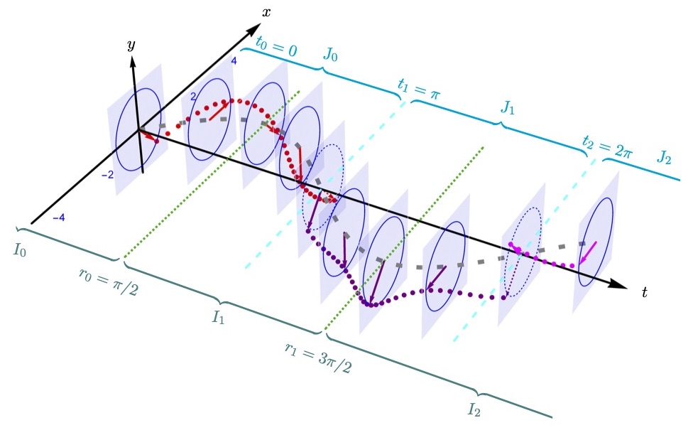
Figure 2: The phase factor ${\bf P}(t)$ of the propagator in (V.1) lies on the unit circle of the complex plane plotted vertically along a classical path $\bar{\gamma}(t)$. The orentation is positive if it is clockwise when seen from $t=+\infty$. In the time interval $J_{\ell}$ labeled by the Maslov index $\ell={\rm Ent}[t/\pi]$, the factor ${\bf P}(t)$ precesses around ${\bf P}_{\ell}=\exp[-i\frac{\pi}{4}(1+2\ell)]$ with double frequency w.r.t. the classical path, $\bar{\gamma}(t)$. Arriving at a caustic the phase jumps by $(-\pi/2)$ (red becoming purple) and then continues until the next caustic when it jumps again (and becomes magenta), and so on.

An intuitive understanding comes by noting that when $t\neq\pi\ell=t_{\ell}$, then different initial velocities $a$ yield classical paths $\bar{x}_{a}(t)$s with different end points, and thus contribute to different propagators. However approaching from the left $\ell$-times a half period, $t\to(\pi\,\ell)-\,,$ all classical paths get focused at the same end-point ($x=0$ for our choice) and for all $a$,

$$P_{a}(t\to\pi\ell-)=e^{-i\frac{\pi}{4}(1+{2}\ell)}\equiv P_{\ell}\,.$$ (V.4)

which is precisely the Maslov phase. Thus all classical paths contribute equally, by $P_{\ell}$, and to the same propagator. Comparing with the right-limit,

$$P_{a}(t\to\pi\ell+)=e^{-i\frac{\pi}{4}(1+{2}(\ell+1)}=P_{\ell+1}=e^{-\frac{i\pi}{2}}P_{\ell}.$$ (V.5)

the Maslov jump is recovered. Choosing instead $y\neq 0$ there will be no classical path from $(0,0)$ to $(y,\pi\ell)$ and thus no contribution to the path integral.

To conclude this section we just mention with that the extended Feynman method HFeynman with the cast $\bar{\omega}$ = constant frequency and $\tau$ = “fake time” would lead also to (IV.3) and (IV.5) with the integer $\ell$ counting the number of negative eigenvalues (Morse index) of the Hessian Schulman ; semiclassic ; Maslov .

V.2 A time-dependent example: the Mathieu equation

The combined Junker-Inomata - Arnold method allows us to go beyond the constant-frequency case, as illustrated here for no friction or driving force, $\lambda=F\equiv 0$, but with explicitly time-dependent frequency. For $\Omega^{2}(t)=a-2q\cos 2t$, for example, (II.4) becomes the Mathieu equation,

$$\ddot{x}+(a-2q\cos 2t)x=0\,.$$ (V.6)

This equation can be solved either analytically using Mathieu functions Mathieuf , or numerically, providing us for $a=2$ and $q=1$ (for which odd Mathieu functions are real) with the dotted curve (in red), shown in Fig.3.

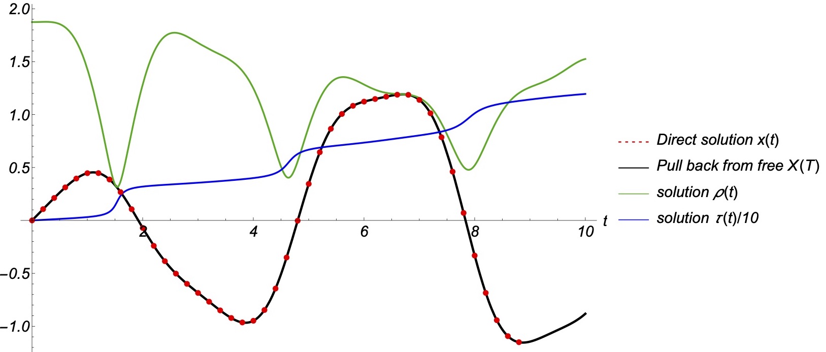
Figure 3: The analytic solution of the Mathieu equation with $a=2,q=1$ for $x(t)$ (dotted in red), lies on the black curve got by (II.5) from combining the numerically obtained $\rho(t)$ (in green) and $\tau(t)$ (in blue), which are solutions of the pair (II.7)-(II.10). The black curve is also obtained by pulling back the free solution (III.19) by the inverse Niederer map (IV.12).

Alternatively, we can use the Junker-Inomata – Arnold transformation (III.17) LopezRuiz ; Arnold . We first achieve $\bar{\omega}=1$ by a redefinition, $\tau\to\tau^{\prime}=\bar{\omega}\tau$. Inserting the Ansatz (II.5) into (V.6) yields the pair of coupled equations (II.6a)-(II.6b). We choose $u_{p}=0$ and two independent solutions $u_{1}(t)$ and $u_{2}(t)$, (III.26), with initial conditions (III.18) with $t_{0}=0$ i.e., $\tau(0)=\dot{\rho}(0)=0,\,\rho(0)=\dot{\tau}(0)=1\,,$ which fix the integration constant, $C=\rho^{2}\left({0}\right)\dot{\tau}({0})=1.$ Then, consistently with the general theory outlined above, the Arnold map (III.17) lifted to Bargmann space becomes (II.11), completed with (III.27) with $\lambda=0$.

Eqn (II.6) is solved by following the strategy outlined in sec.II. Carrying out those steps numerically provides us with Fig.3.

From the general formula (II.13) we deduce, for our choice $x^{\prime\prime}=x,t^{\prime\prime}=t,x^{\prime}=t^{\prime}=0$, the probability density

$$|K(x,t)|^{2}=\frac{\sqrt{\dot{\tau}}}{2\pi\hbar|\sin\tau(t)|}\,,$$ (V.7)

happens not depend on the position, and can therefore be plotted as in Fig.4.

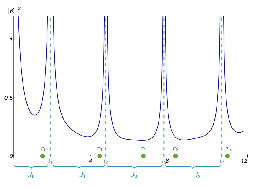
Figure 4: The probability density $|K(x,t)|^{2}$ (V.7) does not depend on $x$ and is regular in each interval ${\color[rgb]{0,1,1}{\bf J}_{\ell}}$ between the adjacent points ${\color[rgb]{0,1,1}\bf t_{\ell}}$ (IV.14), where it diverges. The ${\color[rgb]{0,0.5,0}\bf r_{k}}$ which determine the domains ${\color[rgb]{0,0.5,0}{\bf I}_{k}}$ of the generalized Niederer map (II.11) lie between the ${\color[rgb]{0,1,1}\bf t_{\ell}}$ and conversely.

The propagator $K$ and hence the probability density (V.7) diverge at ${\color[rgb]{0,1,1}\bf t_{\ell}}$, which are roughly $t_{1}\approx 1.92,\,t_{2}\approx 4.80,\,t_{3}\approx 7.83\,.$ The classical motions are regular at the caustics, $\bar{x}(t_{\ell})\propto\rho(t_{\ell})\approx 0,$ see sec. IV. The domains ${\bf I_{k}}=[r_{k-1},r_{k}]$ of the inverse Niederer map are shown in fig.4. Approximately, $r_{1}\approx 1.52,\,r_{2}\approx 4.49,\,r_{3}\approx 6.75,\,r_{4}\approx 8.44\,.$ The evolution of the phase factor along the classical path is depicted in fig.5.

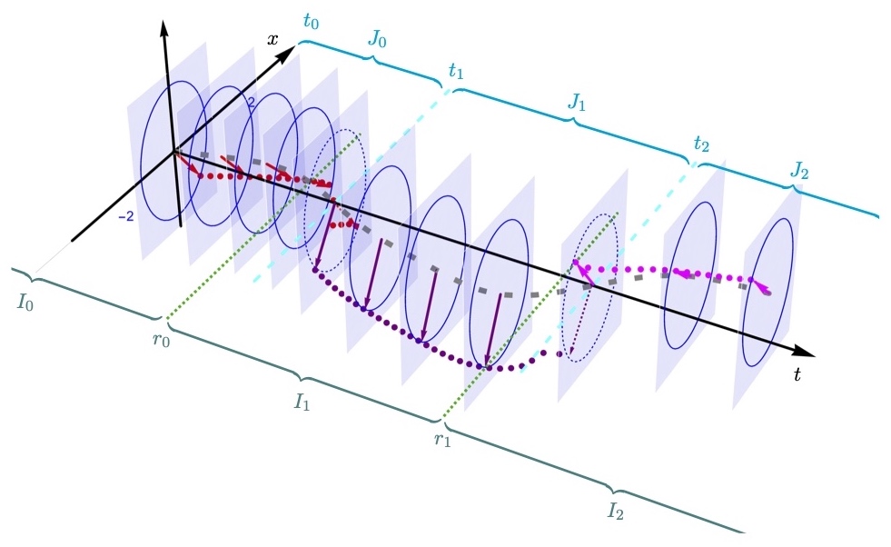
Figure 5: For $0<t<t_{1}$ the Mathieu phase factor ${\bf P}(t)$ plotted along a classical path $\bar{\gamma}(t)=(\bar{x}(t),t)$ precesses around $e^{-i\pi/4}$. Arriving at the caustic point $\tau(t_{1})=\pi$ its phase jumps by $(-\pi/2)$, then oscillates around $e^{-3i\pi/4}$ until $\tau(t_{2})=2\pi$, then jumps again, and so on.

VI Conclusion

The Junker-Inomata – Arnold approach yields (in principle) the exact propagator for any quadratic system by switching from time-dependent to constant frequency and redefined time,

$$\omega(t)\;\to\;\bar{\omega}=\mathop{\rm const.}\nolimits{\quad\text{and}\quad}t\;\to\;\text{``fake time''}\;\;\tau\,.$$ (VI.1)

The propagator (IV.3)-(IV.5) is then derived from the result known for constant frequency. A straightforward consequence is the Maslov jump for arbitrary time-dependent frequency $\omega(t)$ : everything depends only on the product $\bar{\omega}\,\tau$.

By switching from $t$ to $\tau$ the Sturm-Liouville-type difficulty is not eliminated, though, only transferred to that of finding $\tau=\tau(t)$ following the prcedure outlined in sec.II. We have to solve first solve EMP equation (II.7) for $\rho(t)$ (which is non-linear and has time-dependent coefficients), and then integrate $\rho^{-2}$, see (II.10). Although this is as difficult to solve as solving the Sturm-Liouville equation, however it provides us with theoretical insights.

When no analytic solution is available, we can resort to numerical calculations.

The Junker-Inomata approach of sec.II is interpreted as a Bargmann-conformal transformation between time-dependent and constant frequency metrics, see eqn (III.9).

Alternatively, the damped oscillator can be converted to a free system by the generalized Niederer map (II.11), whose Eisenhart-Duval lift (III.17)-(III.21) carries the conformally flat oscillator metric (III.28) to flat Minkowski space.

Two sets of points play a distinguished rôle in our investigations : the $r_{k}$ in (IV.10) and the $t_{\ell}$ in (IV.14). The $r_{k}$ divide the time axis into domains $I_{k}$ of the (generalized) Niederer map (II.11). Both classical motions and quantum propagators are regular at $r_{k}$ where these intervals are joined. The $t_{\ell}$ are in turn the caustic points where all classical trajectories are focused and the quantum propagator becomes singular.

While the “Maslov phase jump” at caustics is well established when the frequency is constant, $\omega=\omega_{0}=\mathop{\rm const.}\nolimits$, its extension to the time-dependent case $\omega=\omega(t)$ is more subtle. In fact, the proofs we are aware of Arnold67 ; SMaslov ; Burdet78 ; RezendeJMP use sophisticated mathematics, or a lengthy direct calculation of the propgagator Cheng87 . A bonus from the Junker-Inomata transcription (I.8) we follow here is to provide us with a straightforward extension valid to an arbitrary $\omega(t)$. Caustics arise when (IV.4) holds, and then the phase jump is given by (IV.27).

The subtle point mentioned above comes from the standard (but somewhat sloppy) expression (I.5) which requires to choose a branch of the double-valued square root function. Once this is done, the sign change of $T^{\prime\prime}-T^{\prime}$ induces a phase jump $\pi/2$. Our “innocently-looking” factor is in fact the Maslov jump for a free particle at $T=0$ (obscured when one considers the propagator for $T>0$ only). Moreover, it then becomes the key tool for the ocillator : intuitively, the multivalued inverse Niederer map repeates, all over again and again, the same jump. Details are discussed in sec.IV.

The transformation (I.8) is related to the non-relativistic “Schrödinger” conformal symmetries of a free non-relativistic particle Jackiw72 ; Niederer72 ; Hagen72 later extended to the oscillator Niederer73 and an inverse-square potential Fubini . These results can in fact be derived using a time-dependent conformal transformation of the type (I.8) BurdetOsci ; GWG_Schwarz .

The above results are readily generalized to higher dimensions. For example, the oscillator frequency can be time-dependent, uniform electric and magnetic fields and a curl-free “Aharonov-Bohm” potential (a vortex line Jackiw90 ) can also be added DHP2 . Further generalization involves a Dirac monopole Jackiw80 .

Alternative ways to relate free and harmonically trapped motions are studied, e.g., in Andr18 ; Inzunza ; Dhasmana . Motions with Mathieu profile are considered also in Guha21 .

- (1) R. P. Feynman and A. R. Hibbs, Quantum Mechanics and path integrals, (McGraw-Hill, N. Y. 1965)
- (2) L. Schulman, Techniques and applications of path integration, (Wiley, N.Y. 1981)
- (3) D. C. Khandekar, S. V. Lawande and K. V. Bhagwat, Path-Integral Methods and Their Applications. 1st edition. World Scientific. Singapore, (1993)
- (4) C. DeWitt-Morette, “The Semiclassical Expansion,” Annals Phys. 97 (1976), 367-399 [erratum: Annals Phys. 101 (1976), 682] doi:10.1016/0003-4916(76)90041-5 S. Levit and U. Smilansky, “A New Approach to Gaussian Path Integrals and the Evaluation of the Semiclassical Propagator,” Annals Phys. 103 (1977), 198 doi:10.1016/0003-4916(77)90269-X
- (5) P. Caldirola, “Forze non-conservative nella meccanica quantistica,” Nuovo Cimento, 18, 393 (1941). E. Kanai, “On the Quantization of the Dissipative Systems” Prog. Theor. Phys., 3, 440 (1948).
- (6) P. A. Horvathy, “Extended Feynman Formula for Harmonic Oscillator,” Int. J. Theor. Phys. 18 (1979), 245 doi:10.1007/BF00671761
- (7) H. Dekker, “Classical and quantum mechanics of the damped harmonic oscillator,” Phys. Rept. 80, 1-112 (1981)
- (8) D. C. Khandekar and S. V. Lawande, “Feynman Path Integrals: Some Exact Results and Applications,” Phys. Rept. 137 (1986), 115-229 doi:10.1016/0370-1573(86)90029-3
- (9) C. I. Um, K. H. Yeon and T. F. George, “The Quantum damped harmonic oscillator,” Phys. Rept. 362 (2002), 63-192 doi:10.1016/S0370-1573(01)00077-1
- (10) G. Junker and A. Inomata, “Transformation of the free propagator to the quadratic propagator,” Phys. Lett. A 110 (1985) 195-198
- (11) P. Y. Cai, A. Inomata and P. Wang, “JACKIW TRANSFORMATION IN PATH INTEGRALS,” Phys. Lett. A 91 (1982), 331-334 doi:10.1016/0375-9601(82)90425-X
- (12) P. Y. Cai, J. M. Cai, & A. Inomata, “A time-dependent conformal transformation in Feynman’s path integral.” In Path integrals from meV to MeV, Bangkok (1989). Virulh Sa-yakanit et al (eds). World Scientific p.279-290. A. Inomata, “Time-dependent conformal transformation in quantum mechanics,” Proc. ISATQP-Shanxi 1992 Ed. J.Q. Liang, M/L. Wang, S.N. Qiao, D.C. Su. Science press (1993) pp. 75-82.
- (13) U. Niederer, “The maximal kinematical invariance group of the harmonic oscillator,” Helv. Phys. Acta 46 (1973), 191-200 PRINT-72-4208.
- (14) L. P. Eisenhart, “Dynamical trajectories and geodesics”, Annals. Math. 30 591-606 (1928).
- (15) C. Duval, G. Burdet, H. P. Kunzle and M. Perrin, “Bargmann Structures and Newton-cartan Theory,” Phys. Rev. D 31 (1985), 1841-1853 doi:10.1103/PhysRevD.31.1841
- (16) G. Burdet, C. Duval; and M. Perrin, “Time Dependent Quantum Systems and Chronoprojective Geometry,” Lett. Math. Phys. 10 (1985), 255-262 doi:10.1007/BF00420564.
- (17) C. Duval, G. W. Gibbons and P. Horvathy, “Celestial mechanics, conformal structures and gravitational waves,” Phys. Rev. D 43 (1991), 3907-3922 doi:10.1103/PhysRevD.43.3907 [arXiv:hep-th/0512188 [hep-th]].
- (18) M. Cariglia, C. Duval, G. W. Gibbons and P. A. Horvathy, “Eisenhart lifts and symmetries of time-dependent systems,” Annals Phys. 373 (2016), 631-654 doi:10.1016/j.aop.2016.07.033 [arXiv:1605.01932 [hep-th]].
- (19) V. I. Arnold, Supplementary Chapters to the Theory of Ordinary Differential Equations (Nauka, Moscow, 1978); Geometrical Methods in the Theory of Ordinary Differential Equations (Springer-Verlag, New York, Berlin, 1983), in English.
- (20) V. P. Maslov, V.C. Bouslaev, V.I. Arnol’d, Théorie des perturbations et méthodes asymptotiques. Dunod, Paris (1972).
- (21) V. I. Arnold, “Characteristic class entering in quantization conditions,” Funktsional’nyi Analiz i Ego Prilozheniya, 1967, 1,1, 1-14, doi:10.1007/BF01075861.
- (22) J. M. Souriau, “Construction explicite de l’indice de Maslov. Applications,” Lect. Notes Phys. 50 (1976), 117-148 doi:10.1007/3-540-07789-8_13
- (23) G. Burdet, M. Perrin, and M. Perroud, “Generating functions for the affine symplectic group,” Comm. Math. Phys. 58 241-254 (1978).
- (24) J. Rezende, “Quantum systems with time dependent harmonic part and the Morse index,”J. Math. Phys. 25 (1984), 32643269 doi:10.1063/1.526073
- (25) V. Aldaya, F. Cossío, J. Guerrero and F.F. López-Ruiz, “The quantum Arnold transformation,” J. Phys. A, 44, 065302 (2011). arXiv:1010.5521 “Symmetries of the quantum damped harmonic oscillator,” J. Phys. A. arXiv:1210.4058 [math-ph]. “Unfolding the quantum Arnold transformation,” Int. J. Geom. Meth. Mod. Phys. 09 (2012) 02, 1260011.
- (26) V. P. Ermakov, “Second order differential equations. Conditions of complete integrability,” Univ. Izv. Kiev, Series III 9 (1880) 1 (English translation: A. O. Harin, under redaction by P. G. L. Leach, Appl. Anal. Discrete Math. 2 (2008) 123, doi:10.2298/AADM0802123E). W. E. Milne, “The numerical determination of characteristic numbers,” Phys. Rev. 35 (1930) 863. E. Pinney, “The nonlinear differential equation ,” Proc. Amer. Math. Soc. 1 (1959) 68.
- (27) A. Galajinsky, “Geometry of the isotropic oscillator driven by the conformal mode,” Eur. Phys. J. C 78 (2018) no.1, 72 doi:10.1140/epjc/s10052-018-5568-8 [arXiv:1712.00742 [hep-th]]. M. Cariglia, A. Galajinsky, G. W. Gibbons and P. A. Horvathy, “Cosmological aspects of the Eisenhart–Duval lift,” Eur. Phys. J. C 78 (2018) no.4, 314 doi:10.1140/epjc/s10052-018-5789-x [arXiv:1802.03370 [gr-qc]].
- (28) B. Cheng, “Exact propagator for the harmonic oscillator with time dependent mass,” Phys. Lett. A 113 (1985), 293 doi:10.1016/0375-9601(85)90166-5
- (29) A. Ilderton, “Screw-symmetric gravitational waves: a double copy of the vortex,” Phys. Lett. B 782 (2018), 22-27 doi:10.1016/j.physletb.2018.04.069 [arXiv:1804.07290 [gr-qc]].
- (30) P. M. Zhang, M. Cariglia, M. Elbistan and P. A. Horvathy, “Scaling and conformal symmetries for plane gravitational waves,” J. Math. Phys. 61 (2020) no.2, 022502 doi:10.1063/1.5136078 [arXiv:1905.08661 [gr-qc]].
- (31) F. F. López-Ruiz and J. Guerrero, “Generalizations of the Ermakov system through the Quantum Arnold Transformation,” J. Phys. Conf. Ser. 538 (2014), 012015 doi:10.1088/1742-6596/538/1/012015
- (32) C. Duval, P. A. Horváthy and L. Palla, “Conformal properties of Chern-Simons vortices in external fields,” Phys. Rev. D50, 6658 (1994). [hep-ph/9405229, hep-th/9404047]
- (33) G. W. Gibbons, “Dark Energy and the Schwarzian Derivative,” [arXiv:1403.5431 [hep-th]].
- (34) Weisstein, E. W. (2003). Mathieu function. https://mathworld. wolfram. com/.
- (35) B. Cheng, “Exact propagator for the one-dimensional time-dependent quadratic Lagrangian,” Lett. Math. Phys. 14 (1987), 7-13 doi:10.1007/BF00403464
- (36) R. Jackiw, “Introducing scale symmetry,” Phys. Today 25N1 (1972), 23-27 doi:10.1063/1.3070673
- (37) U. Niederer, “The maximal kinematical invariance group of the free Schrodinger equation,” Helv. Phys. Acta 45 (1972), 802-810 doi:10.5169/seals-114417
- (38) C. R. Hagen, “Scale and conformal transformations in galilean-covariant field theory,” Phys. Rev. D 5 (1972), 377-388 doi:10.1103/PhysRevD.5.377
- (39) V. de Alfaro, S. Fubini and G. Furlan, “Conformal Invariance in Quantum Mechanics,” Nuovo Cim. A 34 (1976), 569 doi:10.1007/BF02785666
- (40) R. Jackiw, “Dynamical Symmetry of the Magnetic Vortex,” Annals Phys. 201 (1990), 83-116 doi:10.1016/0003-4916(90)90354-Q
- (41) R. Jackiw, “Dynamical Symmetry of the Magnetic Monopole,” Annals Phys. 129 (1980), 183 doi:10.1016/0003-4916(80)90295-X
- (42) K. Andrzejewski and S. Prencel, “Memory effect, conformal symmetry and gravitational plane waves,” Phys. Lett. B 782 (2018), 421-426 doi:10.1016/j.physletb.2018.05.072 [arXiv:1804.10979 [gr-qc]]. “Niederer’s transformation, time-dependent oscillators and polarized gravitational waves,” doi:10.1088/1361-6382/ab2394 [arXiv:1810.06541 [gr-qc]].
- (43) L. Inzunza, M. S. Plyushchay and A. Wipf, “Conformal bridge between asymptotic freedom and confinement,” Phys. Rev. D 101 (2020) no.10, 105019 doi:10.1103/PhysRevD.101.105019 [arXiv:1912.11752 [hep-th]].
- (44) S. Dhasmana, A. Sen and Z. K. Silagadze, “Equivalence of a harmonic oscillator to a free particle and Eisenhart lift,” [arXiv:2106.09523 [quant-ph]].
- (45) P. Guha and S. Garai, “Integrable modulation, curl forces and parametric Kapitza equation with trapping and escaping,” [arXiv:2104.06319 [math-ph]].