An accelerated expectation-maximization algorithm for multi-reference alignment

Abstract

The multi-reference alignment (MRA) problem entails estimating an image from multiple noisy and rotated copies of itself. If the noise level is low, one can reconstruct the image by estimating the missing rotations, aligning the images, and averaging out the noise. While accurate rotation estimation is impossible if the noise level is high, the rotations can still be approximated, and thus can provide indispensable information. In particular, learning the approximation error can be harnessed for efficient image estimation. In this paper, we propose a new computational framework, called Synch-EM, that consists of angular synchronization followed by expectation-maximization (EM). The synchronization step results in a concentrated distribution of rotations; this distribution is learned and then incorporated into the EM as a Bayesian prior. The learned distribution also dramatically reduces the search space, and thus the computational load of the EM iterations. We show by extensive numerical experiments that the proposed framework can significantly accelerate EM for MRA in high noise levels, occasionally by a few orders of magnitude, without degrading the reconstruction quality.

I Introduction

Multi-reference alignment (MRA) is an abstract mathematical model inspired by the problem of constituting a 3-D molecular structure using cryo-electron microscopy (cryo-EM). The MRA problem entails estimating an image from multiple noisy and rotated copies of itself. The computational and statistical properties of the MRA problem have been analyzed thoroughly in recent years, see [7, 6, 20, 4, 2, 19, 13, 5, 3, 23, 1, 11, 16, 9, 18].

This paper focuses on the 2-D MRA model. Let $I$ be an image of size $L\times L$ that we wish to estimate. Let $R_{\theta}$ be a rotation operator which rotates an image counter-clockwise by an angle $\theta$. The observations are i.i.d. random samples drawn from the model:

$$Y=R_{\theta}I+\varepsilon,$$ (1)

where the rotations are drawn from a distribution $\theta\sim\rho$, and $\varepsilon$ is a noise matrix whose entries are i.i.d. Gaussian variables with zero mean and variance $\sigma^{2}$. The variables $\theta$ and $\varepsilon$ are independent. Inspired by cryo-EM, we assume that $\theta$ is distributed uniformly over $\left[0,2\pi\right)$ [8]. The task is to estimate the unknown image $I$ from a set of noisy images $Y_{1},...,Y_{N}$, while the rotations $\theta_{1},...,\theta_{N}$ are unknown. We note that model (1) suffers from an unavoidable ambiguity of rotation, and therefore, naturally, a solution is defined up to a rotation.

Following [19, 30], we assume that the image can be represented in a steerable basis with finitely many coefficients, namely,

$$I(r,\theta)=\sum_{k=-L}^{L}\sum_{q=1}^{p_{k}}{a_{k,q}u^{k,q}(r,\theta)},$$ (2)

where $u^{k,q}(r,\theta)=f^{k,q}(r)e^{\iota k\theta}$ is a steerable basis function in polar coordinates, $f^{k,q}(r)$ is a real valued radial function, $\iota=\sqrt{-1}$, and $p_{k}$ denotes the number of components according to a sampling criterion described in Appendix A. The expansion coefficients are denoted by $a_{k,q}$, where $k,q$ are the angular and radial indices, respectively. Since $u$ is a steerable basis, rotating the image by an angle $\phi$ corresponds to an addition of a linear phase in the coefficients:

$$I(r,\theta-\phi) =\sum_{k=-L}^{L}\sum_{q=1}^{p_{k}}{a_{k,q}u^{k,q}(r,\theta-\phi)}$$ (3)

$$=\sum_{k=-L}^{L}\sum_{q=1}^{p_{k}}{a_{k,q}e^{-\iota k\phi}u^{k,q}(r,\theta)}.$$

As we consider real images, the coefficients satisfy a symmetry, $a_{k,q}=\overline{a_{-k,q}}$, and therefore coefficients with $k\geq 0$ suffice to represent the images. In particular, we use the steerable PCA (sPCA) basis [30], which results in a data driven, steerable, basis to represent the images. In this case, the relation (2) approximately holds; see Appendix A.

Based on our image formation model (2), we reformulate the 2-D MRA problem as follows. Each 2-D MRA observation can be described as:

$$v_{i}=a\circ e^{-\iota\bar{k}\theta_{i}}+\varepsilon^{c}_{i},\quad i=1,\ldots,N,$$ (4)

where $\circ$ denotes entry-wise product, $a$ is the sPCA coefficients vector of the unknown image $I$, $v_{i}$ is the sPCA coefficients vector of the $i$-th observation, $\theta_{i}\in\left[0,2\pi\right)$ is the unknown corresponding rotation, and $\varepsilon_{i}^{c}$ denotes a complex Gaussian vector with i.i.d. entries with zero mean and variance $\sigma^{2}$. We treat the sPCA coefficients $\{v_{k,q}\}$ as a vector $v\in\mathbb{C}^{M}$ such that $v[j]=v_{\bar{k}[j],\bar{q}[j]},\quad j=1,...,M$, where $(\bar{k},\bar{q})\in\mathbb{Z}^{M}$ specify the angular and radial indices at each entry, and $M$ is the number of sPCA coefficients used in the representation. Therefore, given a set of noisy sPCA coefficient vectors $v_{1},...,v_{N},$ corresponding to the noisy images $Y_{1},...,Y_{N}$, we wish to estimate the sPCA coefficients vector $a$ of the unknown image $I$, up to a global rotation. Once the sPCA coefficients vector is estimated, the image can be reconstructed using the sPCA basis.

Previous works on the MRA model focused on two signal to noise (SNR) regimes: high SNR (small $\sigma$) and extremely low SNR ($\sigma\to\infty$). In the sequel, we define $\text{SNR}=\frac{\|I\|_{\text{F}}^{2}}{L^{2}\sigma^{2}}$. In the high SNR regime, one can estimate the unknown rotations using the angular synchronization framework [28, 12, 21, 5]. Then, the observations can be aligned (i.e., undo the rotations) and averaged; see Section II-A for details. However, in very low SNR, accurate rotation estimation is impossible, and thus methods that circumvent rotation estimation were developed and analyzed. In particular, this paper studies expectation-maximization (EM) [14], the most successful methodology for MRA and cryo-EM [24, 27], which is outlined in Section II-B.

In practice, the SNR of cryo-EM data (the main motivation of this work) is not high enough for accurate estimation of rotations, but also not extremely low. A typical SNR ranges between 1/100 to 1/10; this regime is exemplified in Figure 1. In this low (but not extremely low) SNR, synchronization provides indispensable information about the rotations that was neglected by previous works. In particular, while we cannot estimate the rotations accurately, we can estimate the distribution of rotations after synchronization.

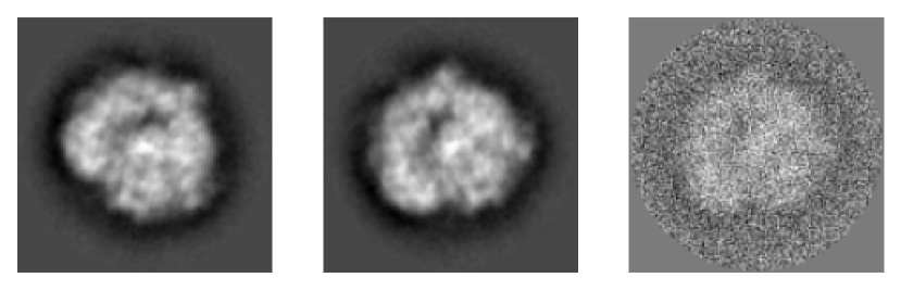
Figure 1: From left to right: The original clean image of a projection image of the E. coli 70S ribosome volume [25], a rotated clean image, and a noisy image with SNR=1/10.

In this paper, we present the Synch-EM framework (see Section III), in which synchronization is incorporated into EM in order to accelerate the reconstruction process. Synchronization helps accelerating EM in three different ways. First, it allows us to find a good initialization point, which is important since the MRA problem (1) is non-convex; similar ideas are also described in the cryo-EM literature [17, 5]. Second, we can establish a meaningful prior information on the distribution of rotations after synchronization. The prior is comprised of a similarity function between the estimated distribution and the expected distribution of rotations, which is learned; see Section III-B for details. Third, if we have confidence that the distribution of rotations is concentrated (depending on the SNR), then we can reduce the search space (occasionally, dramatically), and thus reduce the computational burden; see Section III-C. To mitigate statistical dependencies (discussed in Section III-A1) and to process massive datasets, we also suggest a new synchronization framework, called Synchronize and Match (see Section III-A).

II Image Recovery in High and Low SNR Regimes

This paper focuses on image recovery in the low, but not extremely low, SNR regime. Before presenting the proposed framework, we introduce the classical methods in high and low SNRs and their shortcomings.

II-A High SNR

In high SNR, one can reliably estimate the missing rotations $\theta_{1},...,\theta_{N}$, undo the rotations, and recover the image by averaging. Given any two observations $Y_{i},Y_{j}$ drawn from (1), their relative rotation $\theta_{i,j}$ can be estimated by

$$\hat{\theta}_{i,j}=\arg\min_{\theta\in[0,2\pi)}{\|Y_{i}-R_{-\theta}Y_{j}\|^{2}}.$$ (5)

This can be written in terms of the sPCA coefficients of the images $v^{i}_{k,q}$, $v^{j}_{k,q}$:

$$\hat{\theta}_{i,j}=\arg{\min_{\theta\in[0,2\pi)}{\sum_{k,q}{|v^{i}_{k,q}-e^{\iota k\theta}v^{j}_{k,q}|^{2}}}}.$$ (6)

We now present two methods to estimate rotations.

II-A1 Template matching

A simple, albeit not robust to noise, method to estimate rotations is by template matching. In this method, all observations are aligned with respect to a single reference image. The computational complexity of template matching is $O(NLM)$, where $N$ is the number of observations, $L$ is the number of possible angles (discretization of the unit circle $\left[0,2\pi\right)$), and $M$ is the number of sPCA coefficients. The template matching estimator works well only in high SNR scenarios and tends to be biased; see for example [26], which shows that a reference image (e.g., a portrait of Einstein) can be extracted from pure random noise images.

II-A2 Angular Synchronization

The angular synchronization framework provides a more robust computational paradigm as it considers the ratios between all pairs of images. If the estimated rotations between all pairs are arranged in a matrix $H\in\mathbb{C}^{N\times N}$ such that $H_{i,j}=e^{\iota\hat{\theta}_{i,j}}$, the angular synchronization problem can be associated with the maximum likelihood estimation problem:

$$\max_{z\in\mathbb{C}_{1}^{N}}{z^{*}Hz},$$ (7)

where $\mathbb{C}_{1}^{N}:=\{z\in\mathbb{C}^{N}:|z_{1}|=...=|z_{N}|=1\}$. This is a smooth, non-convex optimization problem on the manifold of product of circles. To solve (7), we follow [12] and apply the projected power method (PPM), which is an iterative algorithms whose $(t+1)$ iteration reads:

$$z^{(t+1)}=\text{phase}(Hz^{(t)}),$$ (8)

where $\text{phase}(z)_{i}=z_{i}/|z_{i}|$. The estimated rotations are then:

$$\hat{\theta}_{i}=\arg{z_{i}}\quad{\color[rgb]{0,0,0}{i=1,...,N}},$$ (9)

where $\arg()$ is the argument of a complex number. The computational complexity of this method is governed by the computation of the relative rotations of all pairs. Since we have $N(N-1)/2$ distinct pairs, the overall complexity is $O(N^{2}LM)$, an order of $N$ higher than template matching. The dependency on $N^{2}$ implies that the computational burden becomes prohibitive for large $N$. Therefore, a modification of the synchronization algorithm must be made in order to process big datasets in a reasonable time.

Once the rotations are estimated (either by template matching or PPM), each image can be easily aligned using the steerability property, $\hat{v}^{i}_{k,q}=e^{\iota k\hat{\theta}_{i}}v^{i}_{k,q}$. Thus, the sPCA coefficients of the image are estimated by averaging the aligned coefficients:

$$\hat{a}_{k,q}=\frac{1}{N}\sum_{i=1}^{N}{e^{\iota k\hat{\theta}_{i}}v^{i}_{k,q}}.$$ (10)

From the estimated sPCA coefficients, one can reconstruct the image using the sPCA basis.

II-B Expectation-maximization

When the SNR is sufficiently low, accurate rotation estimation is impossible. Therefore, in this regime, techniques that estimate the signal directly are used. A popular approach is to maximize the posterior distribution after marginalizing over the rotations:

$$a^{*},\rho^{*}=\arg\max_{a,\rho}p(a,\rho|\boldsymbol{v}),$$ (11)

where $a,\rho$ are, respectively, the unknown image coefficients and the distribution of rotations, and $\boldsymbol{v}=(v_{1},...,v_{N})\in\mathbb{C}^{M\times N}$ is the observation matrix whose $i$-th column corresponds to the sPCA coefficients of the $i$-th observation (4). Recall that (now without marginalizing out the rotations), the posterior distribution is proportional to the likelihood times the prior:

$$p(a,\rho|\boldsymbol{v},\boldsymbol{\theta})\propto p(\boldsymbol{v},\boldsymbol{\theta}|a,\rho)p(a)p(\rho),$$ (12)

where $p(a)$ is the prior on the image coefficients $a$, and $p(\rho)$ is the prior on the distribution of rotations $\rho$, assuming $a$ and $\rho$ are independent. In particular, the likelihood function of 2-D MRA, in terms of sPCA coefficients (4), is given by:

$$p(\boldsymbol{v},\boldsymbol{\theta}|a,\rho)=\prod_{j=1}^{N}\rho[\theta_{j}]\frac{1}{\pi^{M}\sigma^{2M}}e^{-\frac{1}{\sigma^{2}}\|a\circ e^{-\iota{\color[rgb]{0,0,0}{\bar{k}}}\theta_{j}}-v_{j}\|_{2}^{2}}{\color[rgb]{0,0,0}{.}}$$ (13)

Importantly, up to now, the prior on the distribution of rotations $p(\rho)$ was overlooked by previous works in the MRA and cryo-EM literature [24, 7, 2, 19, 10, 27].

The EM algorithm aims to iteratively maximize the marginalized posterior distribution as follows [15]. First, we fix a range of $L$ possible rotations $[0,\frac{2\pi}{L},...,\frac{2\pi(L-1)}{L}]$, according to a required resolution. Then, given a current estimate of the image coefficients $a_{t}$ and distribution $\rho_{t}$, consider the expected value of the log posterior function, with respect to the conditional distribution of $\theta$ given $\boldsymbol{v}$, $a_{t}$ and $\rho_{t}$:

$$Q(a,\rho|a_{t},\rho_{t}) ={\color[rgb]{0,0,0}{\mathbb{E}}}_{\theta|\boldsymbol{v},a_{t},\rho_{t}}\{\log{p(a,\rho|\boldsymbol{v},\boldsymbol{\theta})}\}$$ (14)

$$=\sum_{j=1}^{N}{\sum_{l=0}^{L-1}{w_{t}^{l,j}\{\log\rho[l]-\frac{1}{\sigma^{2}}\|a\circ e^{-\iota\frac{2\pi l}{L}\bar{k}}-v_{j}\|^{2}\}}}$$

$$+\log p(a)+\log p(\rho).$$

The weight $w_{t}^{l,j}$ is the probability that the rotation $\theta_{j}$ of observation $j$ is equal to $\frac{2\pi l}{L}$, given $\boldsymbol{v}$ and assuming $a=a_{t},\rho=\rho_{t}$, and is proportional to:

$$w_{t}^{l,j}\propto e^{-\frac{1}{\sigma^{2}}\|a_{t}\circ e^{-\iota\frac{2\pi l}{L}\bar{k}}-v_{j}\|^{2}}\rho_{t}[l].$$ (15)

Then, $a$ and $\rho$ are updated by:

$$(a_{t+1},\rho_{t+1})=\arg{\max_{a,\rho}{Q(a,\rho|a_{t},\rho_{t})}}.$$ (16)

The EM algorithm iterates between the expectation (14) and the maximization (16) steps until convergence. We assume throughout that the image coefficients were drawn from a complex Gaussian distribution with zero mean and covariance $\Gamma_{a}$ such that $p(a)={1/\left(\pi^{M}\det{(\Gamma_{a})}\right)}\exp(-a^{H}\Gamma_{a}^{-1}a)$, where $(\cdot)^{H}$ denotes the conjugate transpose operator. In this case, the maximizer over the coefficients reads:

$$a_{t+1}=\left(NI+\sigma^{2}\Gamma_{a}^{-1}\right)^{-1}\sum_{j=1}^{N}{\sum_{l=0}^{L-1}{w_{t}^{l,j}e^{\iota\frac{2\pi l}{L}\bar{k}}\circ v_{j}}}.$$ (17)

When there is no prior on the distribution of rotations, the update rule of the distribution reads:

$$\rho_{t+1}[l]=\frac{W_{t}[l]}{\sum_{l=0}^{L-1}{W_{t}[l]}},$$ (18)

where $W_{t}[l]=\sum_{j=1}^{N}{w_{t}^{l,j}}$. The derivations of (17) and (18) are given in Appendix C. The computational complexity of EM is $O(TNLM)$, where $T$ is the number of EM iterations, which tends to increase as the SNR decreases.

Figure 2 shows the relative error as a function of the SNR of EM, template matching, and MRA with known rotations (which is equivalent to averaging i.i.d. Gaussian variables). To account for the rotation symmetry, the relative error between an estimated image $\hat{I}$ and the true image $I$ is defined as:

$$\text{relative error}=\min_{\theta\in[0,2\pi)}\frac{\|R_{\theta}\hat{I}-I\|_{\text{F}}}{\|I\|_{\text{F}}}.$$ (19)

In this experiment, we use projection images of the E. coli 70S ribosome volume taken from [25]. Each image is of size $129\times 129$ pixels. For each SNR value, we ran 10 trials with different projection images and $N=5000$ observations. The rotations were drawn uniformly from a set of 360 possible angles $\frac{2\pi}{360}[1,...,360]$, rather than a continuous range over $\left[0,2\pi\right)$. This allows us to avoid an error floor in high SNR when setting $L=360$. We computed the sPCA coefficients according to [30], in which the number of sPCA coefficients is automatically chosen as a function of the SNR. We ran the EM without a prior on the image coefficients. As can be seen, in the high SNR regime, accurate rotation estimation is possible: the performances of template matching and EM are competitive to the case of known rotations. However, low SNR hampers accurate rotation estimation. In this regime, EM that directly estimates the image outperforms template matching by a large margin.

III Accelarated EM using synchronization

The Synch-EM framework consists of three main ingredients. The first step involves synchronizing the observations. However, synchronization algorithms induce correlations between the signal and the noise terms of the aligned images, which in turn leads to poor performance of the EM (which assumes model (1)). To mitigate this effect, we propose a new synchronization paradigm, called Synchronize and Match (Section III-A). Secondly, the expected distribution of rotations after synchronization is learned (Section III-B1). Finally, an EM algorithm, which takes the learned prior into account, is applied to the synchronized observations. The learned distribution is also used to narrow the search space (Section III-C), leading to a notable acceleration. The framework is outlined in Algorithm 1.

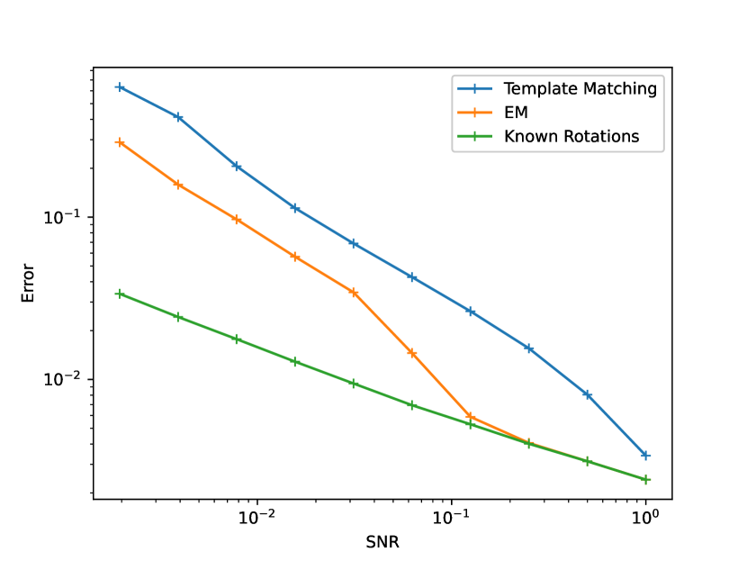
Figure 2: The relative error of template matching, EM and the case of known rotations, in different SNRs, with $N=5000$ samples of 2-D MRA with projection images of the E. coli 70S ribosome.

Algorithm 1 Synch-EM Algorithm

0:  

• $v_{1},...,v_{N}$ - A set of observations drawn from (4)

• $L$ - Number of rotations

• $\overline{\rho}$ - Expected rotation distribution after synchronization learned by Algorithm 3

• $BW$ - Search space bandwidth

• $\gamma$ - Prior weight term

• $\Gamma_{a}$ - The covariance of the image prior

• $tol$ - Tolerance for stopping criteria

• $T$ - Maximum number of iterations

0:  $\hat{I}$ - image estimate

1:  Align the coefficients according to Algorithm 2, resulting in a new set of coefficients $\{{\tilde{v}}_{i}\}_{i=1}^{N}$

2:  Initialize $a_{0}=\frac{1}{N}\sum_{i=1}^{N}{\tilde{v}_{i}}$, $\rho_{0}=\overline{\rho}$

3:  for $t=0$ to $T-1$ do

4:     Compute $w_{t}^{l,j}=\exp{\left(-\frac{1}{\sigma^{2}}\|a_{t}\circ e^{-\iota\frac{2\pi l}{L}\bar{k}}-\tilde{v}_{j}\|^{2}\right)}\rho_{t}[l]$ $\forall l\in[-BW/2,BW/2]$, $\forall j\in[1,...,N]$

5:     Normalize $w_{t}^{l,j}\leftarrow\frac{w_{t}^{l,j}}{{\color[rgb]{0,0,0}{\sum_{l=-BW/2}^{BW/2}}}{w_{t}^{l,j}}}$

6:     Compute $W_{t}[l]=\sum_{j=1}^{N}{w_{t}^{l,j}}$

7:     Update the coefficients

$$a_{t+1}=$$

$$\left(NI+\sigma^{2}\Gamma_{a}^{-1}\right)^{-1}\sum_{j=1}^{N}{{\color[rgb]{0,0,0}{\sum_{l=-BW/2}^{BW/2}}}{w_{t}^{l,j}e^{\iota\frac{2\pi l}{L}\bar{k}}\circ\tilde{v}_{j}}}$$

8:     Update the distribution $\rho_{t+1}[l]=\frac{W_{t}[l]+\gamma\bar{\rho}[l]}{{\color[rgb]{0,0,0}{\sum_{l=-BW/2}^{BW/2}}}{(W_{t}[l]+\gamma\bar{\rho}[l])}}$

9:     if $\min_{l\in[0,L-1]}\|a_{t+1}-e^{-\frac{2\pi\iota\bar{k}l}{L}}\circ a_{t}\|^{2}<tol$ then

10:        break

11:     end if

12:  end for

13:  Reconstruct the estimated image $\hat{I}$ from the estimated sPCA coefficients $a$ and the sPCA basis.

III-A Synchronize and Match

In the first part of this section, we describe how applying synchronization to the data affects the statistical model of the problem. Simulations show that the effect is substantial and leads to poor performance if disregarded. In the second part, we introduce the Synchronize and Match algorithm that was designed to mitigate statistical dependencies induced by synchronization. In addition, it can be applied efficiently to large datasets.

III-A1 Statistical dependencies induced by synchronization

A synchronization algorithm receives a set of observations $Y_{1},...,Y_{n}$ and outputs estimates of their corresponding rotations $\hat{\theta}_{1},...,\hat{\theta}_{N}$ (up to a global rotation). Then, the observations are aligned:

$$\tilde{{\color[rgb]{0,0,0}{Y}}}_{i}=R_{-\hat{\theta_{i}}}(R_{\theta_{i}}{\color[rgb]{0,0,0}{I}}+\varepsilon_{i})=R_{\Delta\theta_{i}}{\color[rgb]{0,0,0}{I}}+\tilde{\varepsilon}_{i},$$ (20)

where $\Delta\theta_{i}=\theta_{i}-\hat{\theta}_{i}$ and $\tilde{\varepsilon}_{i}=R_{-\hat{\theta_{i}}}\varepsilon_{i}$ are the synchronization error and the noise term after alignment, respectively. The distribution of the synchronization error is concentrated (later, in Section III-B1, we explain how this distribution can be learned).

Crucially, since $\hat{\theta}_{i}$ is a function of the unknown rotations, the unknown signal and the noise realizations, the noise term $\tilde{\varepsilon}_{i}$ is not necessarily distributed as $\mathcal{N}(0,\sigma^{2}I)$, and is not necessarily uncorrelated with the signal. To demonstrate that synchronization induces correlation between the noise and the shifted signals, we use the notion of Pearson correlation coefficients. Given a set of pairs of samples $\{(a_{1},b_{1}),...,(a_{N},b_{N})\}$, the Pearson correlation coefficient between $a$ and $b$ is computed by

$$r_{ab}=\frac{\sum_{i=1}^{N}{(a_{i}-\bar{a})(b_{i}-\bar{b})}}{\sqrt{\sum_{i=1}^{N}{(a_{i}-\bar{a})^{2}}\sum_{i=1}^{N}{(b_{i}-\bar{b})^{2}}}},$$ (21)

where $\bar{a}$ and $\bar{b}$ are, respectively, the sample mean of $a$ and $b$. Under the assumption that $a$ and $b$ are drawn independently from normal distributions, the variable $t=r\sqrt{\frac{N-2}{1-r^{2}}}$ follows a Student’s t-distribution with $N-2$ degrees of freedom. This also holds approximately for other distributions with large enough sample size. This allows us to check whether $a$ and $b$ are independent variables with some prescribed significance level (say, $\alpha=0.05$).

For this demonstration, and to avoid the effects of change of basis, we use the 1-D discrete version of (1). In this case, the sought signal is a 1-D discrete vector $x\in\mathbb{R}^{L}$, and $R_{\theta}$ is a circular shift operator where the shifts are uniformly distributed over $[0,...,L-1]$. Here we use a signal of length $L=21$, whose entries were drawn independently from a normal distribution with zero mean and unit variance. We set $\sigma=2$ and $N=1000$. For each MRA trial, we computed the Pearson coefficient between each entry of the shifted signal and the noise before synchronization: $r_{R_{s}x[i],\varepsilon[j]}$, $\forall i,j\in[0,L-1]$. We repeated the experiment for 20 trials. As expected, we measured a fraction of 0.048 of Pearson coefficients whose p-values are smaller than 0.05. This verifies that the shifted signal and the noise entries, before synchronization, are indeed uncorrelated. Then, we repeated the same experiment with the shifted signal and the noise after angular synchronization, using PPM. As can be seen in Figure 3, more entries have large Peasron coefficients, indicating that they are unlikely to be uncorrelated. We measured a fraction of 0.205 of Pearson coefficients whose p-values are smaller than 0.05. Therefore, we conclude that the shifted signal and noise are correlated after synchronization.

To remedy the correlation problem, this paper suggests a new synchronization method, introduced in the following section, called Synchronize and Match. Conducting the same experiment with this method alleviates the induced correlation: we measured a fraction of 0.102 Pearson coefficients whose p-values are smaller than 0.05.

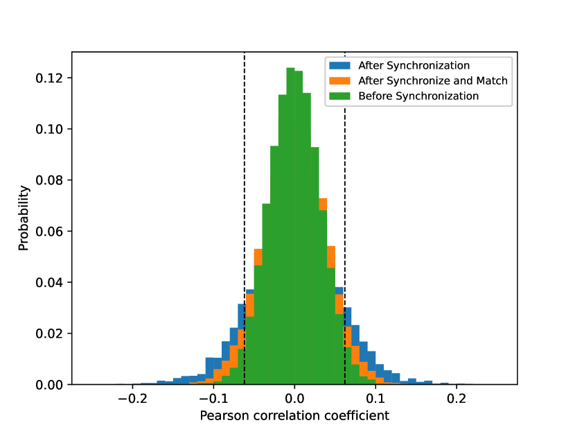
Figure 3: Correlation can be detected using the Pearson correlation test. The panel shows normalized histograms of the Pearson correlation coefficients between the shifted signal and noise, before and after synchronization. The dashed vertical lines correspond to a significance level of $\alpha=0.05$ according to the Student’s t-distribution. The experiment confirms that while the shifted signal and noise before synchronization are uncorrelated, synchronization introduces a significant amount of correlation between them. Synchronize and Match (Algorithm 1) alleviates this problem.

Figure 4 shows the relative error as a function of SNR of EM, template matching followed by EM, and angular synchronization using PPM followed by EM. In this 1-D MRA experiment, we used a signal of length $L=21$ whose entries were drawn independently from a normal distribution with zero mean and unit variance. For each SNR, we ran 10 trials with $N=500$. Notice how the correlation induced by synchronization degrades the performance of EM (which assumes the model (1)).

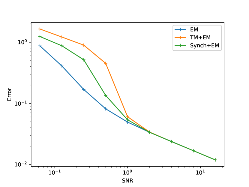
Figure 4: Degraded performance of EM after alignment, due to correlations induced by synchronization. In blue, standard EM; in orange, template matching followed by EM (TM+EM); and in green, angular synchronization using PPM followed by EM (Synch+EM).

III-A2 Synchronize and Match

Synchronization induces correlation between the shifted signal and the noise because each rotation estimation depends on the measurement’s specific noise realization. To weaken the correlation, the key idea of the Synchronize and Match algorithm is partitioning the data into two subsets of size $P$ and $N-P$, with $P\ll N$. Let us denote these sets by $S_{P}$ and $S_{N-P}$. Synchronization is applied only to $S_{P}$ (the small subset), resulting in $P$ rotation estimations. Next, we assign to each image in $S_{N-P}$ the rotation assigned to its closest neighbor in $S_{P}$ (whose rotation was estimated in the previous step). Finally, in order to break the dependency between the estimated rotations and the noise within $S_{P}$, each image in $S_{P}$ is assigned with the rotation corresponding to its closest image in $S_{P}$, excluding itself. The algorithm is outlined in Algorithm 2.

Algorithm 2 Synchronize and Match

0:  A set of observed sPCA coefficients $v_{1},...,v_{N}$ corresponding to $Y_{1},...,Y_{N}$ and partition size $P\ll N$

0:  $\hat{\theta}_{i}\quad\forall i\in[1,N]$

1:  Partition the data into two subsets, $S_{P}=\{{\color[rgb]{0,0,0}{v}}_{i}\}_{i=1}^{P}$ and $S_{N-P}=\{{\color[rgb]{0,0,0}{v}}_{i}\}_{i=P+1}^{N}$.

2:  Apply synchronization to $S_{P}$ using the projected power method (see Section II-A2), resulting in a set of rotation estimates $\hat{\phi}_{1},,...,\hat{\phi}_{P},$ corresponding to ${\color[rgb]{0,0,0}{v}}_{1},,...,{\color[rgb]{0,0,0}{v}}_{P}$.

3:  for $i=P+1$ to $N$ do

4:     $\hat{\theta}_{i}=\hat{\phi}_{\arg\min_{n\in[1,P]}{\|{\color[rgb]{0,0,0}{v}}_{i}-{\color[rgb]{0,0,0}{v}}_{n}\|_{2}^{2}}}$

5:  end for

6:  for $i=1$ to $P$ do

7:     $\hat{\theta}_{i}=\hat{\phi}_{\arg\min_{n\in[1,P],n\neq i}\|v_{i}-v_{n}\|_{2}^{2}}$

8:  end for

The synchronization of the small set has a complexity of $O(P^{2}LM)$, while the complexity of assigning rotations to the second set is $O((N-P)PM)$. Thus, for $N\gg PL$ the complexity is dominated by $O(PMN)$. The parameter P controls a trade-off between runtime and accuracy. $P$ should be chosen to be large enough such that the distribution of rotations will be concentrated, but should be kept low such that the runtime of Synchronize and Match will be negligible compared to the EM.

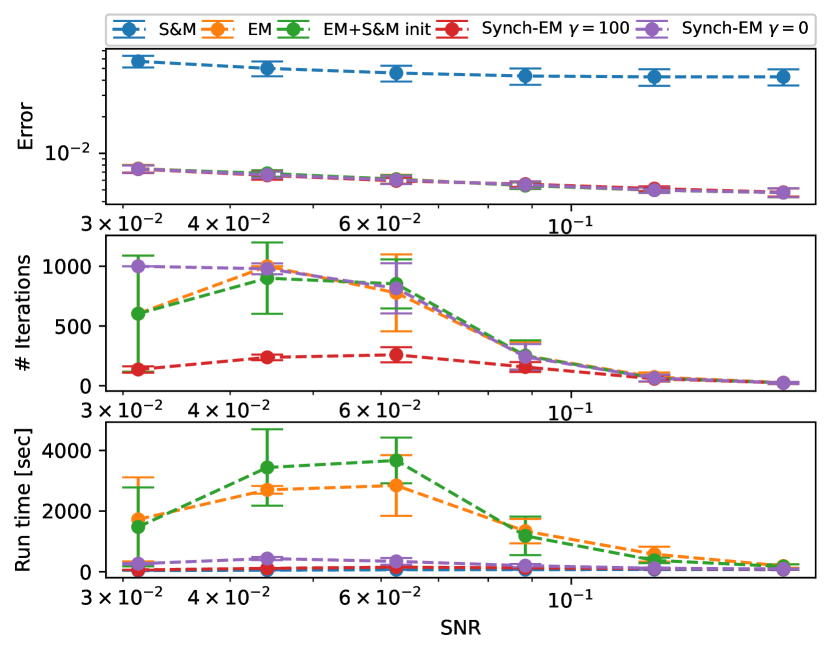
Figure 10: Performance of Synchronize and Match (S&M), standard EM with random initialization (EM), standard EM initialized from the average of the aligned coefficients after S&M (EM+S&M init), and Synch-EM with different distribution prior weighting (Synch-EM $\gamma=100$ and $\gamma=0$), as a function of the SNR, with $N=5000$ and a signal prior, averaged over 10 trials.

The synchronization step allows us to initialize the EM from the average of the aligned coefficients $a_{0}=\frac{1}{N}\sum_{i=1}^{N}{{v}_{i}}$, rather than a random guess. This initialization is required for the reduced search space to function properly. Even though EM in general is sensitive to initialization, the initialization by itself does not contribute to the speed up of the EM process. This is demonstrated in Figures 6, 7, 8, 9 and 10, in which standard EM with an initial guess equals to the averaged aligned coefficients (denoted as EM+S&M init) is compared against standard EM with a random guess.

III-B Establishing prior on the distribution of rotations

We are now turning our attention to learning the expected distribution of rotations after synchronization. This will allow us to incorporate this essential information into the EM iterations as a prior, and to narrow down the search space. It is important to note that the expected distribution depends on the specific synchronization method that is being used (in our case, Synchronize and Match), the SNR, and the unknown image. Since it seems to be out of reach to compute this distribution analytically, we introduce a learning methodology to learn the expected distribution of rotations. In Appendix B, we provide an approximation for the expected distribution of 1-D MRA using template matching as a synchronization method with a known reference signal. Once the expected distribution is learned, we show how to incorporate it into the EM iterations as a prior in the Bayesian sense.

III-B1 Learning methodology

Since synchronization estimates rotations up to some global rotation $\theta_{c}$, we are interested in the expected distribution of the centered rotation error $\Delta\bar{\theta}=\hat{\theta}-\theta-\theta_{c}$, which can be formulated as:

$$p_{\Delta\bar{\theta}}[l]=\mathbb{E}_{\boldsymbol{\theta},\boldsymbol{\varepsilon},x}\left[\frac{1}{N}\sum_{j=1}^{N}\mathcal{I}_{\left\lfloor\frac{\Delta\bar{\theta}_{j}L}{2\pi}\right\rfloor=l}\right],$$ (22)

where $\theta\sim\mathcal{U}\left[0,2\pi\right)$, $\varepsilon\sim\mathcal{N}(0,\sigma^{2}I)$, $x\sim p(x)$, and $\mathcal{I}$ is the indicator function. The suggested algorithm approximates (22) using Monte-Carlo simulations by computing the sample mean of the measured centered distribution of rotations after synchronization of different trials, for a given noise variance $\sigma^{2}$ and number of observations $N$. The process is detailed in Algorithm 3.

Algorithm 3 Algorithm for learning rotation distribution

0:   • $p(x)$ - signal prior • $\sigma^{2}$ - noise variance • $N$ - number of observations • $f$ - synchronization method • $L$ - number of possible rotations • $R$ - number of repetitions

0:  Estimated expected centered distribution of rotations after synchronization $\bar{\rho}[l],l\in[0,L-1]$

1:  for $r=1$ to $R$ do

2:     Draw $x$ from $p(x)$

3:     Generate $Y_{1},...,Y_{N}$ according to (1), with $\theta_{1},...,\theta_{N}$ distributed uniformly over $\left[0,2\pi\right)$

4:     Estimate $\hat{\theta}_{1},...,\hat{\theta}_{N}$ using synchronization $\hat{\boldsymbol{\theta}}=f(y_{1},...,y_{N})$

5:     Compute the global rotation between the estimated rotations and the signal $\theta_{c}=\arg\min_{\theta}\|R_{\theta}\{\frac{1}{N}\sum_{j=1}^{N}R_{-\hat{\theta}_{j}}Y_{j}\}-x\|^{2}$

6:     Compute the rotation error $\Delta\bar{\theta}_{i}=\hat{\theta_{i}}-\theta_{i}-\theta_{c}\quad i=0,\ldots,N-1$

7:     Compute $\hat{\rho}_{r}[l]=\frac{1}{N}\sum_{i=0}^{N-1}{\mathcal{I}_{\left\lfloor\frac{\Delta\bar{\theta}_{j}L}{2\pi}\right\rfloor=l}},\quad l=0,\ldots,L-1$

8:  end for

9:  $\bar{\rho}[l]=\frac{1}{R}\sum_{r=1}^{R}{\hat{\rho}_{r}[l]},\quad l=0,\ldots,L-1$

Figure 5 shows an example of the learned distribution of rotations after synchronization, using the Synchronize and Match algorithm, with $N=500$, $L=360$, with $R=50$ repetitions, and $x$ is drawn from a set of 10 projection images of the E. coli 70S ribosome volume taken from [25]. Evidently. the learned distribution becomes more concentrated as the SNR increases. This allows us to narrow down the search space of the following EM iterations, thus reducing its computational load.

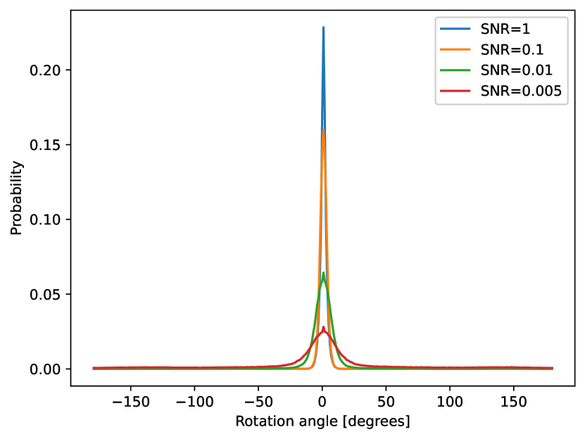
Figure 5: Learned distribution of rotations using Algorithm 3 in different SNRs.

III-B2 Prior on the distribution of rotations

The prior reflects how we model the distribution of rotations around the expected distribution, which was learned using Algorithm 3. Specifically, once the expected distribution of rotations after synchronization $\bar{\rho}$ is learned, we assume that the probability of a measured distribution of rotations $\rho$ is:

$$p(\rho)\propto e^{-\gamma{\color[rgb]{0,0,0}{D_{KL}(\bar{\rho},\rho)}}},$$ (23)

where $\gamma$ is a regularizer term and

$$D_{KL}(\bar{\rho},\rho)=\sum_{l=0}^{L-1}{\bar{\rho}[l]\log{\frac{\bar{\rho}[l]}{\rho[l]}}}.$$ (24)

In Appendix C we derive the update rule of the estimated distribution in the EM iterations (16) using this prior, that is used in Algorithm 1.

III-C Reduced search space

As demonstrated in Figure 5, even in rather low SNR values, the range of likely rotations remains small. This allows us to reduce the search space from all possible rotations (because of the uniform distribution of rotations in (1)) to a much narrower space of likely rotations after synchronization.

Suppose that we consider L equally spaced possible rotations. Namely, the EM iterations search over the angles $\left[0,{\color[rgb]{0,0,0}{\frac{2\pi}{L}}},...,\frac{2\pi(L-1)}{L}\right]$. If the expected distribution is indeed narrow, it allows us to consider a smaller set of angles $\left[-\frac{\pi BW}{L},-\frac{\pi BW+2\pi}{L},...,\frac{\pi BW}{L}\right]$ for $BW\leq L$. $BW$ should be chosen according to the SNR and the learned distribution. For example, in the experiment of Figure 5 with SNR=1/100, one can set $BW=36$ with only negligible loss of information. Similarly, one can retain the same computational load while increasing resolution by sampling the range of likely rotations more densely $\left[-\frac{\pi BW}{L},-\frac{\pi(L-1)BW}{L^{2}},...,\frac{\pi(L-1)BW}{L^{2}},\frac{\pi BW}{L}\right]$, with the appropriate modification of the EM.

IV Numerical Experiments

In this section, we compare Algorithm 1 to standard EM applied to the statistical model (1) (see, for example, [7]) in different scenarios. We use projection images of the E. coli 70S ribosome volume taken from [25]. Each image is of size $129\times 129$ pixels. The code to reproduce all experiments (including those presented in previous sections) is publicly available at https://github.com/noamjanco/synch-em.

IV-A Performance without signal prior

We first examine the Synch-EM algorithm without taking into account the signal prior $p(a)$ within the EM iterations. Figures 6, 7 and 8 compare the relative error, number of iterations and runtime of Synchronize and Match, standard EM with random initialization, standard EM initialized from the average of the aligned coefficients after Synchronize and Match, and Synch-EM with different distribution prior weighting, as a function of the SNR, for $N=1000$, $N=5000$ and $N=10000$, respectively. For each SNR, the results were averaged over 10 trials. We used $L=360$, $P=100$, $\gamma=100$, a fixed $BW=36$, $T=1000$, and $tol=10^{-5}$. The runtime of Synch-EM includes Synchronize and Match. Table I also presents a runtime comparison for $N=10000$ for the SNRs of interest. There is a clear and significant improvement in runtime of Synch-EM compared to standard EM in all scenarios, which gets more significant as $N$ increases. The improvement in runtime results from two compounding affects: the computational burden of each EM iteration is reduced due to the narrower search space after synchronization, and the reduced number of EM iterations (for $N=5000$ and $N=10000$) in the low SNRs (lower than 1/10). We see that as $N$ increases, the reduction in the number of iterations is more significant. For example, for $N=10000$ (Figure 8) and $\text{SNR}=1/16$, the average number of iterations using standard EM was 699, compared to 221 using Synch-EM. The average running time using standard EM was 7064 seconds, compared to 166 seconds using Synch-EM. We also see that the choice of $BW=36$ has a negligible effect on the accuracy, unless the SNR is below 1/100.

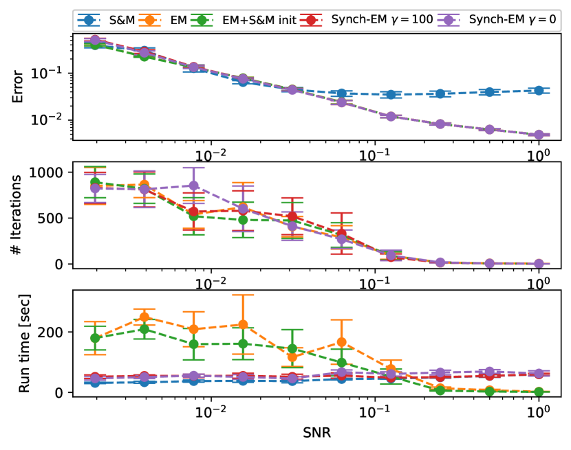
Figure 6: Performance of Synchronize and Match (S&M), standard EM with random initialization (EM), standard EM initialized from the average of the aligned coefficients after S&M (EM+S&M init), and Synch-EM with different distribution prior weighting (Synch-EM $\gamma=100$ and $\gamma=0$), as a function of the SNR, with $N=1000$, averaged over 10 trials.

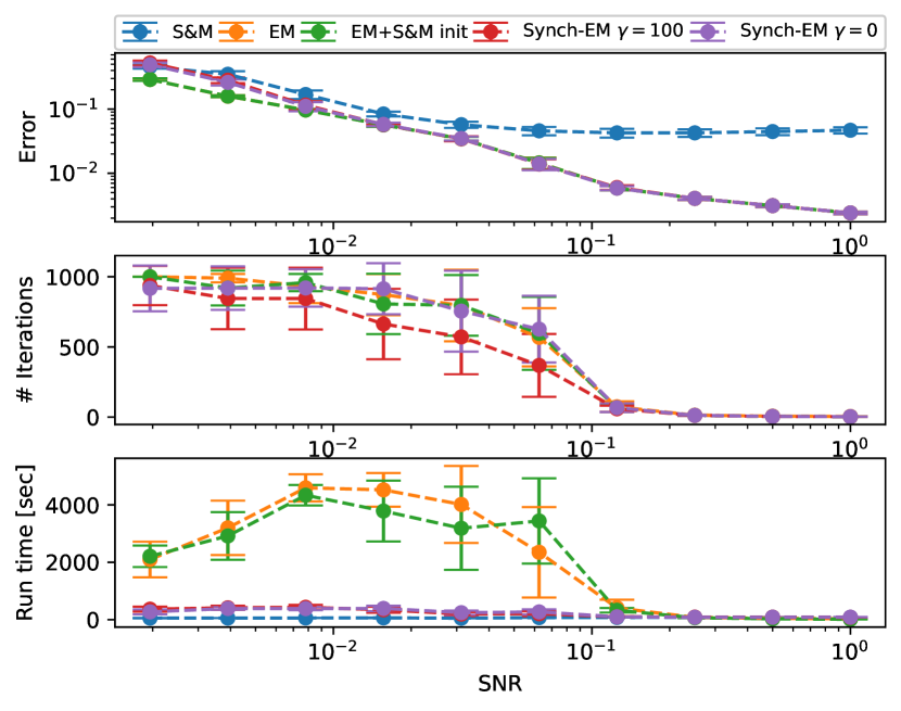
Figure 7: Performance of Synchronize and Match (S&M), standard EM with random initialization (EM), standard EM initialized from the average of the aligned coefficients after S&M (EM+S&M init), and Synch-EM with different distribution prior weighting (Synch-EM $\gamma=100$ and $\gamma=0$), as a function of the SNR, with $N=5000$, averaged over 10 trials.

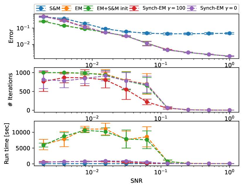
Figure 8: Performance of Synchronize and Match (S&M), standard EM with random initialization (EM), standard EM initialized from the average of the aligned coefficients after S&M (EM+S&M init), and Synch-EM with different distribution prior weighting (Synch-EM $\gamma=100$ and $\gamma=0$), as a function of the SNR, with $N=10000$, averaged over 10 trials.

SNR	$1/8$	$1/16$	$1/32$	$1/64$
Synchronize and Match	93	85	74	73
EM	746	8564	7681	11031
EM + S&M init	776	7624	7865	10179
Synch-EM $\gamma=100$	133	205	552	759
Synch-EM $\gamma=0$	127	534	844	913

TABLE I: Runtime in seconds comparison of Synchronize and Match, standard EM with random initialization (EM), standard EM initialized from the average of the aligned coefficients after S&M (EM+S&M init), and Synch-EM with different distribution prior weighting (Synch-EM $\gamma=100$ and $\gamma=0$), as a function of the SNR, with $N=10000$.

IV-B Performance with signal prior

We repeated the same experiment with an explicit signal prior $p(a)$ incorporated into the EM iterations, in both standard EM and Synch-EM. The signal prior assumes that $a\sim\mathcal{CN}(0,\Gamma_{a})$, where $\Gamma_{a}$ is a diagonal covariance matrix whose entries decay exponentially with the angular frequency of the sPCA coefficient: $\Gamma_{a}=\text{diag}((4e^{-\bar{k}/8})^{2})$. The decay parameters were empirically fitted based on 20 clean projection images of the E. coli 70S ribosome volume taken from [25]. Figures 9 and 10 present the relative error, number of iterations and runtime of standard EM, Synchronize and Match, and Synch-EM, for $N=1000$ and $N=5000$, respectively. Table II also presents a runtime comparison for $N=5000$ for the SNRs of interest. We notice that the signal prior improves the relative error of both standard EM and Synch-EM, which outperform synchronization (compare, for example, SNR=0.03 in Figure 6 and Figure 9). The error of both algorithms remains quite low in low SNRs. Again, we see a significant improvement in runtime due to the reduced number of iterations and the narrow search space in the SNRs of interest (below 1/10).

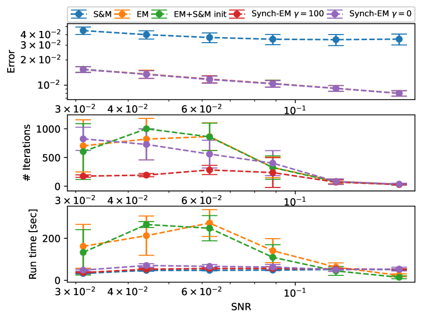
Figure 9: Performance of Synchronize and Match (S&M), standard EM with random initialization (EM), standard EM initialized from the average of the aligned coefficients after S&M (EM+S&M init), and Synch-EM with different distribution prior weighting (Synch-EM $\gamma=100$ and $\gamma=0$), as a function of the SNR, with $N=1000$ and a signal prior, averaged over 10 trials.

SNR	$0.125$	$0.0883$	$0.0625$	$0.0441$
Synchronize and Match	74	69	65	51
EM	579	1339	2844	2699
EM + S&M init	375	1183	3669	3437
Synch-EM $\gamma=100$	102	128	151	112
Synch-EM $\gamma=0$	115	200	342	435

TABLE II: Runtime in seconds comparison of Synchronize and Match, standard EM with random initialization (EM), standard EM initialized from the average of the aligned coefficients after S&M (EM+S&M init), and Synch-EM with different distribution prior weighting (Synch-EM $\gamma=100$ and $\gamma=0$), as a function of the SNR, with $N=5000$ and a signal prior.

The choice of the explicit signal prior affects both standard EM and Synch-EM. In the following experiment, we evaluated the relative error, number of iterations and runtime of standard EM and Synch-EM, for different choices of the decay parameter $\beta$ in the assumed signal coefficient’s covariance $\Gamma_{a}=\text{diag}((4e^{-\bar{k}/\beta})^{2})$. Figure 11 shows the results of the experiment, with $N=5000$ observations and 10 trials for each SNR level. The experiment verifies our choice of $\beta=8$, and also shows that the choice of the signal prior has a similar effect on the relative error performance of both the standard EM and the Synch-EM.

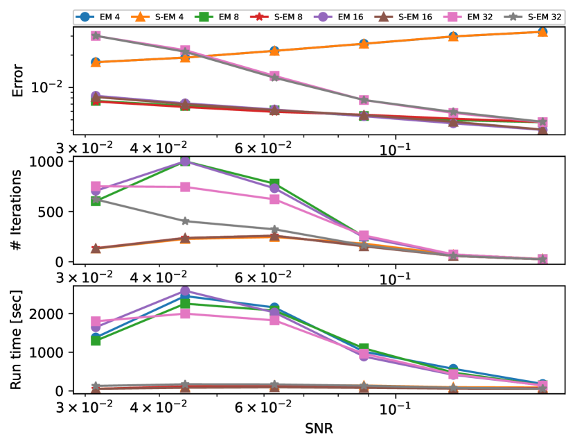
Figure 11: Performance comparison between standard EM (EM) and Synch-EM (S-EM) over different choices of signal prior. The label describes the decay parameter $\beta$ in the assumed covariance of signal’s coefficients $\Gamma_{a}=\text{diag}((4e^{-\bar{k}/\beta})^{2})$, with $N=5000$ observations. For example, EM 4 refers to standard EM with $\beta=4$ and S-EM 4 refers to Synch-EM with $\beta=4$, averaged over 10 trials.

IV-C Prior weighting

In this experiment, we demonstrate how different values of $\gamma$, the weight of the prior on the distribution of rotations after synchronization, affect the EM. In this experiment we used $L=360$, $P=100$, $BW=36$, $T=1000$, $tol=10^{-5}$, $N=5000$, and no explicit signal prior. Figure 12 shows the relative error and number iterations of Synch-EM as a function of SNR, for $\gamma=0,1,10,100$. For each SNR, the results were averaged over 10 trials. The case of $\gamma=0$ corresponds to having no prior on the distribution of rotations after synchronization (besides the reduced search space). As can be seen, the prior reduces the number of EM iterations for values greater than 0, for low SNR values, without increasing the relative error.

Figure 12: Performance of Synch-EM with different values of $\gamma$: the weight of the prior on the distribution of rotations. We see that non-zero weight reduces the number of iterations in low SNR.

IV-D Performance with different BW

In the last experiment we tested different choices of BW on the relative error performance. Figure 13 shows the relative error as a function of different $BW$ values with $N=10000$ samples, with signal prior, for different SNR levels. The experiment indicates that the error does not decrease for BW greater than 32. Another interesting phenomena is that for specific working regimes (for example $\text{SNR}=0.0884$, $BW=16$) we get a slight improvement in the relative error. This improvement can be explained by fact that the reduced search space acts as a smoothing prior since it does not allow rotations far from the initial guess.

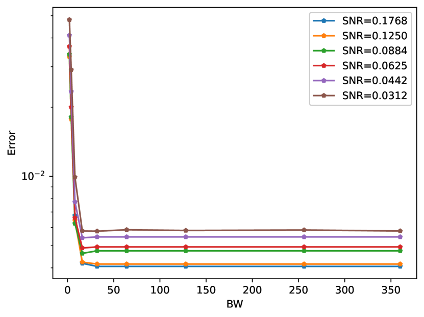
Figure 13: Error as a function of the parameter $BW$ with signal prior for different SNR levels.

V Conclusions and potential implications to cryo-EM

In this paper, we have presented the Synch-EM framework, where a modified synchronization algorithm is incorporated into EM. This framework introduces three features that provide significant runtime acceleration. First, the synchronization algorithm approximates the image, and this approximation can be used to initialize the EM. Second, it allows establishing a prior on the distribution of rotations after synchronization. Third, since the distribution of rotations after synchronization tends to be concentrated (unless the SNR is very low), the search space can be narrowed down, thus reducing the computational burden. In the SNR range between 1/100 to 1/10, we achieve a significant improvement in runtime, without compromising accuracy.

The recent interest in the MRA model, and this paper in specific, is mainly motivated by the emerging technology of cryo-EM to reconstruct 3-D molecular structures [8]. We now outline how the Sync-EM framework can be extended, in principle, to cryo-EM datasets. Under some simplifying assumptions, a cryo-EM experiment results in a series of images, modeled as

$$I_{i}={h}\ast T_{t_{i}}PR_{\omega_{i}}\phi+\varepsilon_{i},\quad i=1,...,N{\color[rgb]{0,0,0}{,}}$$ (25)

where $\phi:\mathbb{R}^{3}\to\mathbb{R}$ is a representation of the 3-D structure to be recovered, $R_{\omega}$ is a 3-D rotation by $\omega\in\text{SO}(3)$, P is a fixed tomographic projection, $T_{t}$ is a 2-D shift by $t\in\mathbb{R}^{2}$, $h$ is the point spread function of the microscope, and $\varepsilon\sim\ \mathcal{N}(0,\sigma^{2}I)$ is an additive noise. To estimate $\phi$ from the images $I_{1},\ldots,I_{N}$, popular software packages implement the EM algorithm [24, 22]. Notably, all packages in the field assume a uniform prior over the distribution of 3-D rotations.

Similarly to the 2-D MRA model (1), there is an established technique to estimate the 3-D rotations from cryo-EM images [29]. However, since it is impossible to estimate rotations accurately in low SNR (the SNR in cryo-EM datasets can be as low as 1/100), it is used only to construct low-resolution ab initio models [17, 5]. A modified version of Algorithm 1 can be designed to learn the expected distribution after synchronization, and to narrow down the search space. Importantly, since EM for cryo-EM samples the group of 3-D rotations SO(3) (rather than SO(2) in (1)), restricting the search space might lead to dramatic acceleration, far exceeding the acceleration factor presented in this paper. In addition, Sync-EM can be combined with other techniques which are currently used to narrow the search space along the EM iterations [24, 22].

Appendix A Fourier-Bessel Basis and Steerable PCA

Before applying steerable PCA (sPCA), we expand all observable images $Y_{1},...,Y_{N}$ in Fourier-Bessel basis, which is a steerable basis. The Fourier-Bessel basis on a disk with radius $c$ is defined as:

$$u^{k,q}(r,\theta)=\begin{cases}N_{k,q}J_{k}(R_{k,q}\frac{r}{c})e^{\iota k\theta},&r\leq c\\ 0,&r>c\end{cases},$$ (26)

where $J_{k}$ is the Bessel function of the first kind, $R_{k,q}$ is the $q^{th}$ root of $J_{k}$ and $N_{k,q}=(c\sqrt{\pi}|J_{k+1}(R_{k,q})|)^{-1}$ is a normalization factor [19], [30]. We take $c$ to be $(L-1)/2$ according to the support of the images.

We assume that the true image can be represented accurately using these components:

$$I(r,\theta)=\sum_{k=-L}^{L}\sum_{q=1}^{p_{k}}{a_{k,q}u^{k,q}(r,\theta)},$$ (27)

where $p_{k}$ denotes the number of components, determined by a sampling criterion (the analog of Nyquist sampling Theorem) that dictates $R_{k,q}\leq\pi L/2$ [31].

The process of computing the Fourier-Bessel coefficients [30] is done first by sampling the continuous Fourier-Bessel basis per pixel within the circle of radius $L/2$ from the center of the image:

$$U^{k,q}(x,y)=u^{k,q}(r(x,y),\theta(x,y)).$$ (28)

The matrix $U^{k,q}$ per pixel is rearranged as a vector, and each vector per pixel is placed as a row in a matrix $\Psi^{\prime}\in\mathbb{C}^{N\times M^{\prime}}$, where $N$ is the number of pixels within the circle, and $M^{\prime}$ is the number of pairs of angular and radial frequencies used in the representation. Given an image in the pixel space $I$ and using (2), the Fourier Bessel coefficients are computed as the least square solution: $\alpha^{*}=\min_{\alpha}{\|\Psi^{\prime}\alpha-I\|_{2}^{2}}=(\Psi^{\prime*}\Psi^{\prime})^{-1}\Psi^{\prime*}I$. Note that $\Psi^{\prime\dagger}=(\Psi^{\prime*}\Psi^{\prime})^{-1}\Psi^{\prime*}$ can be computed once and then applied to the observations (in parallel). We also note that although the Fourier-Bessel functions are orthogonal as continuous functions, their discrete sampled versions on Cartesian grid are not necessarily orthogonal. However, they approach orthogonality as $L\to\infty$ [31]. Numerical observations suggest that for moderate values of $L$ this approximation holds. This means that the white noise remains approximately white after the transformation, which allows us to reformulate the problem as in (4).

Then, to reduce the dimensionality of the representation and to denoise the image, sPCA is applied [30]. The sPCA results in a new data driven basis $\Psi\in\mathbb{C}^{N\times M}$ to represent the images, while preserving the steerability property. The number of sPCA coefficients being used $M<M^{\prime}$ is automatically chosen as a function of the SNR [30]. Finally, all observable images $Y_{1},...,Y_{N}$ are expanded in the sPCA basis, which results in a set of observable coefficients $v_{1},...,v_{N}$, where $v_{i}\in\mathbb{C}^{M}$.

Appendix B An approximation of the Distribution of Shifts in a toy problem

We are interested in the error distribution of the estimated shifts in 1-D MRA, where the shift estimation is performed using template matching with the true signal as the reference signal. We assume $x\in\mathbb{R}^{L}$ drawn from $\mathcal{N}(0,I)$. To ease notation, we consider the case where the MRA observations have zero shift. We wish to estimate the probability mass function $p_{\theta}[m]=p(\theta=m)$ of the discrete random variable $\theta$, defined by:

$$\theta=\arg\max_{l\in[0,L-1]}R_{xy}[l],$$ (29)

where $R_{xy}[l]={\sum_{n=0}^{L-1}{x[n]y[(n+l)\bmod L]}}$. Assuming zero shift, $y\sim\mathcal{N}(x,\sigma^{2}I)$, and $R_{xy}[l]=R_{xx}[l]+\sum_{n=0}^{L-1}x[n]\varepsilon_{i}[(n+l)\bmod{L}]$. Thus, $R_{xy}\sim\mathcal{N}(R_{xx},\Sigma)$, and

$$\Sigma_{i,j}=\sigma^{2}\sum_{l=0}^{L-1}x[l]x[l+j-i\bmod L],$$ (30)

with diagonal entries $\Sigma_{i,i}=\sigma^{2}\|x\|^{2}:=\sigma_{c}^{2}$. The probability of estimating a shift $m$ is the probability of the event in which the correlation between $x$ and $y$ at entry $m$ was greater than all other entries. In other words, the PMF of the estimated shifts is:

$$p(m)=\text{Prob}\left(R_{xy}[m]>\max_{\begin{subarray}{c}n\\ n\neq m\end{subarray}}R_{xy}[n]\right).$$ (31)

In general, $\Sigma$ is not a diagonal matrix. However, since $x\sim\mathcal{N}(0,I)$, we can approximate $\Sigma$ (for large L) by $\Sigma\approx\sigma_{c}^{2}I$. Under this approximation, it follows that the elements of $R_{xy}$ are independent, with $R_{xy}[j]\sim\ \mathcal{N}(R_{xx}[j],\sigma_{c}^{2})$. Let us denote $A_{m}=R_{xy}[m]$ and $B_{m}=\max_{\begin{subarray}{c}n\\ n\neq m\end{subarray}}A_{n}$. Thus, the probability density function of $A_{m}$ is:

$$f_{A_{m}}(u)=\frac{1}{\sqrt{2\pi\sigma_{c}^{2}}}e^{-\frac{(u-R_{xx}[m])^{2}}{2\sigma_{c}^{2}}},$$ (32)

and the cumulative distribution function is

$$F_{A_{m}}(u)=\frac{1}{2}+\frac{1}{2}erf\left({\frac{u-R_{xx}[m]}{\sqrt{2\sigma_{c}^{2}}}}\right).$$ (33)

Since we assumed that the random variables $A_{0},...,A_{L-1}$ are independent, the cumulative distribution function of $B_{m}$, their maximum excluding $A_{m}$, is given by:

$$F_{B_{m}}(u)=P\left(B_{m}<u\right)=\prod_{\begin{subarray}{c}n=0\\ n\neq m\end{subarray}}^{L-1}{F_{A_{n}}(u)}.$$ (34)

Since $A_{m}$ and $B_{m}$ are independent, $f_{A_{m},B_{m}}(u,v)=f_{A_{m}}(u)f_{B_{m}}(v)$, and thus

$$P\left(A_{m}>B_{m}\right)=\int_{-\infty}^{\infty}f_{A_{m}}(u)\int_{-\infty}^{u}{f_{B_{m}}(v)dv}du.$$ (35)

Using the cumulative distribution function, we can also write:

$$\begin{aligned} P\left(A_{m}>B_{m}\right)=\int_{-\infty}^{\infty}{f_{A_{m}}(u)F_{B_{m}}(u)du}\end{aligned}.$$ (36)

Substituting (32), (33) and (34) into (36) yields:

$$\begin{aligned} p_{\theta}[m]\approx\int_{-\infty}^{\infty}{\frac{1}{\sqrt{2\pi\sigma_{c}^{2}}}e^{-\frac{(u-R_{xx}[m])^{2}}{2\sigma_{c}^{2}}}}\times\\ {\prod_{\begin{subarray}{c}l=0\\ l\neq m\end{subarray}}^{L-1}{\left(\frac{1}{2}+\frac{1}{2}erf\left({\frac{u-R_{xx}[l]}{\sqrt{2\sigma_{c}^{2}}}}\right)\right)}du}\end{aligned}.$$ (37)

Figure 14 shows the approximated distribution and the empirical distribution for a single realization of $x$, with $L=21$ and $\sigma=3$. The empirical distribution was computed using $100,000$ samples.

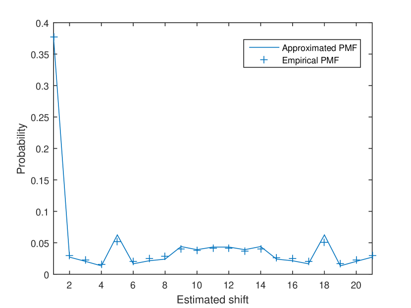
Figure 14: Approximated distribution (computed analytically according to (37)) for a single known realization of $x$, with $L=21$ and $\sigma=3$, compared against the empirical distribution.

Figure 15 shows the mean squared error between the empirical distribution (computed over 100,000 samples) and the approximated distribution (computed analytically according to (37)), averaged over 10 different signal realizations, as a function of $L$ for $\sigma=3$. The average is taken across the different shifts and realizations. As can be seen, the approximation gets better as $L$ increases.

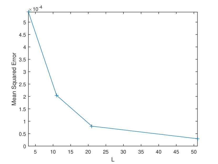
Figure 15: Mean squared error between the approximated distribution (computed analytically according to (37)) and the empirical distribution.

Appendix C M-Step for MAP-EM with prior on the distribution

In this section, we derive the maximization step $(a_{t+1},\rho_{t+1})=\arg{\max_{a,\rho}{Q(a,\rho|a_{t},\rho_{t})}}$, where $Q$ is given by (14). By substituting the prior on the distribution of rotations given in Section III-B2, the Lagrangian is given by:

$$\mathcal{L}(\rho,\lambda)=$$ (38)

$$\sum_{l=0}^{L-1}{W_{t}[l]\log{\rho[l]}}-\gamma\sum_{l=0}^{L-1}{\bar{\rho}[l]\log{\frac{\bar{\rho}[l]}{\rho[l]}}}-\lambda\left(\sum_{l=0}^{L-1}{\rho[l]}-1\right).$$

Setting the derivatives to zero yields

$$\frac{\partial\mathcal{L}(\rho,\lambda)}{\partial\rho[l]}=\frac{W_{t}[l]}{\rho[l]}+\gamma\frac{\bar{\rho}[l]}{\rho[l]}-\lambda=0.$$ (39)

Solving for $\rho$:

$$\rho[l]=\frac{1}{\lambda}(W_{t}[l]+\gamma\overline{\rho}[l]).$$ (40)

Differentiating by $\lambda$ and equating to zero:

$$\frac{\partial\mathcal{L}(\rho,\lambda)}{\partial\lambda}=\sum_{l=0}^{L-1}{\rho[l]}-1=0,$$ (41)

which enforces that $\rho$ is normalized to one. By substituting (40) into (41), we get $\lambda=\sum_{l=0}^{L-1}{(W_{t}[l]+\gamma\bar{\rho}[l])}$, which results in:

$$\rho_{t+1}[l]=\frac{W_{t}[l]+\gamma\bar{\rho}[l]}{\sum_{l=0}^{L-1}{(W_{t}[l]+\gamma\bar{\rho}[l])}}.$$ (42)

Maximizing over $a$ with $a\sim\ \mathcal{CN}(0,\Gamma_{a})$ results in:

$$a_{t+1}=\arg\min_{a}\sigma^{2}a^{H}\Gamma_{a}^{-1}a+\sum_{j=1}^{N}{\sum_{l=0}^{L-1}w_{t}^{l,j}\|a\circ e^{-\iota\frac{2\pi l}{L}\bar{k}}-v_{j}\|^{2}}.$$ (43)

Setting the derivative to zero and solving for $a$ yields:

$$a_{t+1}=\left(NI+\sigma^{2}\Gamma_{a}^{-1}\right)^{-1}\sum_{j=1}^{N}{\sum_{l=0}^{L-1}{w_{t}^{l,j}e^{\iota\frac{2\pi l}{L}\bar{k}}\circ v_{j}}}.$$ (44)

References

- [1] Asaf Abas, Tamir Bendory, and Nir Sharon. The generalized method of moments for multi-reference alignment. IEEE Transactions on Signal Processing, 2022.
- [2] E. Abbe, T. Bendory, W. Leeb, J. M. Pereira, N. Sharon, and A. Singer. Multireference alignment is easier with an aperiodic translation distribution. IEEE Transactions on Information Theory, 65(6):3565–3584, 2019.
- [3] Afonso S Bandeira, Ben Blum-Smith, Joe Kileel, Amelia Perry, Jonathan Weed, and Alexander S Wein. Estimation under group actions: recovering orbits from invariants. arXiv preprint arXiv:1712.10163, 2017.
- [4] Afonso S Bandeira, Moses Charikar, Amit Singer, and Andy Zhu. Multireference alignment using semidefinite programming. In Proceedings of the 5th conference on Innovations in theoretical computer science, pages 459–470, 2014.
- [5] Afonso S Bandeira, Yutong Chen, Roy R Lederman, and Amit Singer. Non-unique games over compact groups and orientation estimation in cryo-EM. Inverse Problems, 36(6):064002, 2020.
- [6] Afonso S Bandeira, Jonathan Niles-Weed, and Philippe Rigollet. Optimal rates of estimation for multi-reference alignment. Mathematical Statistics and Learning, 2(1):25–75, 2020.
- [7] T. Bendory, N. Boumal, C. Ma, Z. Zhao, and A. Singer. Bispectrum inversion with application to multireference alignment. IEEE Transactions on Signal Processing, 66:1037–1050, 2018.
- [8] Tamir Bendory, Alberto Bartesaghi, and Amit Singer. Single-particle cryo-electron microscopy: Mathematical theory, computational challenges, and opportunities. IEEE Signal Processing Magazine, 37(2):58–76, 2020.
- [9] Tamir Bendory, Dan Edidin, William Leeb, and Nir Sharon. Dihedral multi-reference alignment. IEEE Transactions on Information Theory, 2022.
- [10] Tamir Bendory, Ariel Jaffe, William Leeb, Nir Sharon, and Amit Singer. Super-resolution multi-reference alignment. Information and Inference: A Journal of the IMA, 2021.
- [11] Tamir Bendory, Oscar Mickelin, and Amit Singer. Sparse multi-reference alignment: sample complexity and computational hardness. arXiv preprint arXiv:2109.11656, 2021.
- [12] Nicolas Boumal. Nonconvex phase synchronization. SIAM Journal on Optimization, 26(4):2355–2377, 2016.
- [13] Nicolas Boumal, Tamir Bendory, Roy R Lederman, and Amit Singer. Heterogeneous multireference alignment: A single pass approach. In 2018 52nd Annual Conference on Information Sciences and Systems (CISS), pages 1–6. IEEE, 2018.
- [14] A. P. Dempster, N. M. Laird, and D. B. Rubin. Maximum likelihood from incomplete data via the EM algorithm. Journal of the Royal Statistical Society. Series B (Methodological), 39:1–38, 1977.
- [15] Arthur P Dempster, Nan M Laird, and Donald B Rubin. Maximum likelihood from incomplete data via the em algorithm. Journal of the Royal Statistical Society: Series B (Methodological), 39(1):1–22, 1977.
- [16] Subhro Ghosh and Philippe Rigollet. Multi-reference alignment for sparse signals, uniform uncertainty principles and the beltway problem. arXiv preprint arXiv:2106.12996, 2021.
- [17] Ido Greenberg and Yoel Shkolnisky. Common lines modeling for reference free ab-initio reconstruction in cryo-EM. Journal of structural biology, 200(2):106–117, 2017.
- [18] Allen Liu and Ankur Moitra. How to decompose a tensor with group structure. arXiv preprint arXiv:2106.02680, 2021.
- [19] C. Ma, T. Bendory, N. Boumal, F. Sigworth, and A. Singer. Heterogeneous multireference alignment for images with application to 2-D classification in single particle reconstruction. IEEE Transactions on Image Processing, 29:1699–1710, 2020.
- [20] Amelia Perry, Jonathan Weed, Afonso S Bandeira, Philippe Rigollet, and Amit Singer. The sample complexity of multireference alignment. SIAM Journal on Mathematics of Data Science, 1(3):497–517, 2019.
- [21] Amelia Perry, Alexander S. Wein, Afonso S. Bandeira, and Ankur Moitra. Message-passing algorithms for synchronization problems over compact groups. Communications on Pure and Applied Mathematics, 71(11):2275–2322, Apr 2018.
- [22] Ali Punjani, John L Rubinstein, David J Fleet, and Marcus A Brubaker. cryoSPARC: algorithms for rapid unsupervised cryo-EM structure determination. Nature methods, 14(3):290–296, 2017.
- [23] Elad Romanov, Tamir Bendory, and Or Ordentlich. Multi-reference alignment in high dimensions: sample complexity and phase transition. SIAM Journal on Mathematics of Data Science, 3(2):494–523, 2021.
- [24] Sjors HW Scheres. RELION: implementation of a Bayesian approach to cryo-EM structure determination. Journal of structural biology, 180(3):519–530, 2012.
- [25] Tanvir R Shaikh, Haixiao Gao, William T Baxter, Francisco J Asturias, Nicolas Boisset, Ardean Leith, and Joachim Frank. SPIDER image processing for single-particle reconstruction of biological macromolecules from electron micrographs. Nature Protocols, 3(12):1941–1974, October 2008.
- [26] Maxim Shatsky, Richard J. Hall, Steven E. Brenner, and Robert M. Glaeser. A method for the alignment of heterogeneous macromolecules from electron microscopy. Journal of Structural Biology, 166(1):67–78, April 2009.
- [27] Fred J Sigworth. A maximum-likelihood approach to single-particle image refinement. Journal of structural biology, 122(3):328–339, 1998.
- [28] Amit Singer. Angular synchronization by eigenvectors and semidefinite programming. Applied and computational harmonic analysis, 30(1):20–36, 2011.
- [29] Amit Singer and Yoel Shkolnisky. Three-dimensional structure determination from common lines in cryo-EM by eigenvectors and semidefinite programming. SIAM journal on imaging sciences, 4(2):543–572, 2011.
- [30] Zhizhen Zhao, Yoel Shkolnisky, and Amit Singer. Fast steerable principal component analysis. IEEE Transactions on Computational Imaging, 2(1):1–12, 2016.
- [31] Zhizhen Zhao and Amit Singer. Fourier–Bessel rotational invariant eigenimages. JOSA A, 30(5):871–877, 2013.