Ambiguity Rate of Hidden Markov Processes

Abstract

The $\epsilon$-machine is a stochastic process’ optimal model—maximally predictive and minimal in size. It often happens that to optimally predict even simply-defined processes, probabilistic models—including the $\epsilon$-machine—must employ an uncountably-infinite set of features. To constructively work with these infinite sets we map the $\epsilon$-machine to a place-dependent iterated function system (IFS)—a stochastic dynamical system. We then introduce the ambiguity rate that, in conjunction with a process’ Shannon entropy rate, determines the rate at which this set of predictive features must grow to maintain maximal predictive power. We demonstrate, as a ancillary technical result which stands on its own, that the ambiguity rate is the (until now missing) correction to the Lyapunov dimension of an IFS’s attractor. For a broad class of complex processes and for the first time, this then allows calculating their statistical complexity dimension—the information dimension of the minimal set of predictive features.

I Introduction

An abiding challenge to scientific inquiry is the nature of complex systems—those that create intricate and delicate patterns through their internal interplay of stochasticity and determinism. These systems are often identified by the presence intrinsic instabilities, collectively-interacting subsystems, and visually-striking emergent structures.

Integrating Turing’s computation theory [1, 2, 3], Shannon’s information theory [4], and Kolmogorov’s dynamical systems theory [5, 6, 7, 8, 9], computational mechanics [10] introduced a suite of tools to analyze complex systems in terms of their informational architecture. The $\epsilon$-machine—its most basic statistic—is a system’s maximally predictive, minimal, and unique model. It captures a system’s generation, storage, and transmission of information. Quantitatively, the information stored in the $\epsilon$-machine’s causal states—the minimal set of maximally-predictive features—is a process’ statistical complexity $C_{\mu}$, a measure of the memory resources a system employs to generate its behavior and organization.

An optimally predictive model can be imagined as a minimally noisy channel communicating the system’s future into the past. The student of information theory will recall that Shannon, in his analysis of information transmission through channels, introduced two mechanisms: equivocation, in which the same input may lead to distinct outputs, and ambiguity, in which two different inputs may lead to the same output; see Fig. 1. When our channel is taken to be the $\epsilon$-machine, the equivocation rate of the channel is the entropy rate $h_{\mu}$ of the underlying system—the rate at which the system generates future information. This is guaranteed by the predictive optimality of the $\epsilon$-machine—the only noise in the channel is due to the intrinsic randomness of our complex system.

In the following, we introduce the parallel quantity, the ambiguity rate $h_{a}$. The ambiguity rate tracks the rate at which the system discards past information by introducing uncertainty over the infinite past. Explicitly, if a process can be optimally modeled with a finite set of predictive features, its $\epsilon$-machine must forget information at the same rate at which the system generates it: $h_{\mu}=h_{a}$. However, this is atypical, as our predecessor works demonstrated [11, 12]. In point of fact, for many complex systems, the predictive-feature set is uncountably infinite and the statistical complexity $C_{\mu}$ diverges, requiring the development of new tools to characterize the complexity of these systems.

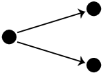
(a)        (b)

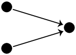
Figure 1: (a) Equivocation: Same input sequence leads to different outputs. (b) Ambiguity: Two different inputs lead to same output. The strategy underlying Shannon’s proof of his second coding theorem is to find channel inputs that are least ambiguous given the channel’s distortion properties, which include equivocation.

The recent work introduced a suite of tools to capture this state of affairs for a broad class of stochastic processes—those used not only in the study of complex systems [10], but also in coding theory [13], stochastic processes [14], stochastic thermodynamics [15], speech recognition [16], computational biology [17, 18], epidemiology [19], and finance [20].

The key realization was identifying a process’ $\epsilon$-machine as the attractor of a hidden Markov-Driven Iterated Function System (DIFS) [11]. First, we showed that this gave efficient and accurate calculation of a process’ Shannon entropy rate $h_{\mu}$. Second, we introduced a new measure of structural complexity—the statistical complexity dimension $d_{\mu}$—that tracks $C_{\mu}$’s divergence and gives the information dimension of the distribution of predictive features [12].

Previously, accurate calculation of $d_{\mu}$ was contingent on the DIFS meeting restrictive technical conditions. Introducing ambiguity rate $h_{a}$ reframes these constraints information-theoretically, effectively lifting them. The result is a new method to accurately calculate $d_{\mu}$ for a broad class of complex processes. More abstractly, we propose $h_{a}$ as a new intrinsic complexity measure of a stochastic process—the growth rate of the information stored in a process’ optimally predictive features. When $h_{\mu}=h_{a}$, this growth rate vanishes and the associated $\epsilon$-machine’s internal causal-state process is stationary. However, when $h_{\mu}>h_{a}$, the latter process is nonstationary and any optimal predictor must accumulate new information over time to sustain accurate predictions.

Our development below introduces and motivates the ambiguity rate $h_{a}$. Sections II and III review stochastic processes and information theory, respectively, and may be skipped by the familiar reader. Section IV introduces hidden Markov-driven iterated function systems. Section V then discusses the statistical complexity dimension $d_{\mu}$ and the overlap problem—a long-standing issue in the dimension theory of iterated function systems. Section VI introduces $h_{a}$ from an information-theoretic perspective, motivating it as a solution to and a measure of the overlap problem. Various interpretations are explored, including an historical note on Shannon’s original dimension rate from 1948. Finally, to illustrate our algorithm’s effectiveness and the challenges for very complex processes, Section VII works through multiple example processes, including those generated by stationary and nonstationary $\epsilon$-machines.

II Processes

A stochastic process $\mathcal{P}$ is a probability measure over a bi-infinite chain $\ldots\,{X}_{t-2}\,{X}_{t-1}\,{X}_{t}\,{X}_{t+1}\,{X}_{t+2}\ldots$ of random variables, each ${X}_{t}$ denoted by a capital letter. A particular realization $\ldots\,{x}_{t-2}\,{x}_{t-1}\,{x}_{t}\,{x}_{t+1}\,{x}_{t+2}\ldots$ is denoted via lowercase. We assume values ${x}_{t}$ belong to a discrete alphabet $\mathcal{A}$. We work with blocks ${X}_{t:t^{\prime}}$, where the first index is inclusive and the second exclusive: ${X}_{t:t^{\prime}}={X}_{t}\ldots{X}_{t^{\prime}-1}$. $\mathcal{P}$’s measure is defined via the collection of distributions over blocks: $\{\Pr({X}_{t:t^{\prime}}):t<t^{\prime},t,t^{\prime}\in\mathbb{Z}\}$.

To simplify, we restrict to stationary, ergodic processes: those for which $\Pr({X}_{t:t+\ell})=\Pr({X}_{0:\ell})$ for all $t\in\mathbb{Z}$, $\ell\in\mathbb{Z}^{+}$, and for which individual realizations obey all of those statistics. In such cases, we only need to consider a process’s length-$\ell$ word distributions $\Pr({X}_{0:\ell})$.

A Markov process is one for which $\Pr({X}_{t}|{X}_{-\infty:t})=\Pr({X}_{t}|{X}_{t-1})$. A hidden Markov process is the output of a memoryless channel [21] whose input is a Markov process [14].

III Information Theory

Beyond its vast technological applications to communication systems [21], Shannon’s information theory [4] is a widely-used foundational framework that provides tools to describe how stochastic processes generate, store, and transmit information. In particular, we use information theory to study complex systems as it makes minimal assumptions as to the nature of correlations between random variables and handles multi-way, nonlinear correlations that are common in complex processes. Here, we now briefly recall several concepts needed in the following.

Information theory’s most basic measure is the Shannon entropy. Intuitively, it is the amount of information that one gains when observing a sample of a random variable. Equivalently modulo sign, it is also the amount of uncertainty one faces when predicting the sample. The entropy $H[{X}]$ of the random variable ${X}$ is:

$$H[{X}]=-\sum_{{x}\in\mathcal{A}}\Pr({X}={x})\log_{2}\Pr({X}={x})~{}.$$ (1)

We can probe the relationship between two jointly-distributed random variables, say, ${X}$ and $Y$. There is the joint entropy $H[{X},Y]$, of the same functional form but applied to the joint distribution $\Pr({X},Y)$. And, there is conditional entropy that gives the amount of information learned from observation of one random variable given another:

$$H[{X}|Y]=H[{X},Y]-H[Y]~{}.$$ (2)

Conditional entropy can be generalized to describe processes in terms of the intrinsic randomness—the amount of information one learns upon observing the next emitted symbol $X_{0}$, given complete knowledge of the infinite past. This is the Shannon entropy rate:

$$h_{\mu}=\lim_{\ell\to\infty}H[{X}_{0}|{X}_{-\ell:0}]~{},$$ (3)

the irreducible amount of information gained in each time step.

The fundamental measure of correlation between random variables is the mutual information. It can be written in terms of Shannon entropies:

$$I[{X};Y]=H[{X},Y]-H[{X}|Y]-H[Y|{X}]~{}.$$ (4)

As should be clear by inspection, the mutual information between two variables is symmetric. When ${X}$ and $Y$ are independent, the mutual information between them vanishes. As with entropy, we may condition the mutual information on another random variable, giving the conditional mutual information:

$$I[{X};Y|Z]=H[{X}|Z]+H[Y|Z]-H[{X},Y|Z]~{}.$$ (5)

The conditional mutual information is the amount of information shared by ${X}$ and $Y$, given we know a third, $Z$. Note that ${X}$ and $Y$ can share mutual information, but be conditionally independent. Moreover, conditioning on a third variable $Z$ can either increase or decrease mutual information [21]. That is, two variables can appear more or less dependent, given additional data.

IV driven iterated function system

Our main objects of study are hidden Markov processes. The following introduces driven iterated function system as a class of predictive models for them. A given hidden Markov process can have many alternative models, each is referred to as a presentation. Driven iterated functions systems are one class of presentations.

Definition 1.

An $N$-dimensional hidden Markov-driven iterated function system (DIFS) $\left(\mathcal{A},\mathcal{V},\bm{\mathcal{R}},\{T^{({x})}\},\{p^{({x})}\},\{f^{({x})}\}:{x}\in\mathcal{A}\right)$ consists of:

1. a finite alphabet $\mathcal{A}$ of $k$ symbols $x\in\mathcal{A}$,

2. a set $\mathcal{V}$ of $N$ presentation states,

3. a set of states $\bm{\mathcal{R}}\subset\Delta^{(N-1)}$, over $N$-dimensional presentation-state distributions $\eta\in\bm{\mathcal{R}}$,

4. a finite set of $N$ by $N$ symbol-labeled substochastic matrices $T^{({x})}$, ${x}\in\mathcal{A}$,

5. a set of $k$ symbol-labeled probability functions $p^{({x})}=\langle\eta|T^{({x})}{\mathbf{1}}\rangle$, and

6. a set of $k$ symbol-labeled mapping functions $f^{({x})}=\langle\eta|T^{({x})}{\mathbf{1}}\rangle/p^{({x})}(\eta)$.

The (N-1)-simplex $\Delta^{N-1}$ is the set of presentation-state probability distributions such that:

$$\{\eta\in\mathbb{R}^{N}:\langle\eta\ket{{\mathbf{1}}}=1,\langle\eta\ket{\delta_{i}}\geq 0,i=1,\dots,N\}~{},$$

where $\bra{\delta_{i}}=\begin{pmatrix}0&0&\dots&1&\dots&0\end{pmatrix}$—that is, $\bra{\delta_{i}}_{i}=1$, otherwise $0$—and $\ket{{\mathbf{1}}}=\begin{pmatrix}1&1&\dots&1\end{pmatrix}$. We use this notation for components of the presentation-state vector $\eta$ to avoid confusion with temporal indexing.

Figure 2: How a hidden Markov-driven iterated function system (DIFS) generates a hidden Markov process: An initial state $\eta$—a distribution over three states: $(0,0,1)$, $(0,1,0)$, and $(1,0,0)$—in the $2$-simplex is associated with a transition probability distribution $p^{x}(\eta)$ over the alphabet ${x}\in\mathcal{A}=\{\square,\triangle\}$. If the emitted symbol selected from this distribution is $\square$, the next state is generated according to the associated mapping function $f^{(\square)}(\eta)$ and the probability distribution is updated accordingly. The same steps are followed if the symbol is $\triangle$ using $f^{(\triangle)}(\eta)$, resulting in an emitted process $\mathcal{P}$ over symbols $\mathcal{A}$.

The set of substochastic matrices must sum to the nonnegative, row-stochastic matrix $T=\sum_{{x}\in\mathcal{A}}T^{({x})}$—the transition matrix for the presentation-state Markov chain. This ensures that $\sum_{{x}\in\mathcal{A}}p^{({x})}(\eta)=1$ for all $\eta\in\Delta^{(N-1)}$.

Figure 2 shows how a DIFS generates a hidden Markov process: Given an initial state $\eta_{0}\in\Delta^{N-1}$, the probability distribution $\{p^{({x})}(\eta_{0}):{x}=1,\dots,k\}$ is sampled. According to the realization ${x}_{0}$, apply the mapping function to map $\eta_{0}$ to the next state $\eta_{1}=f^{({x}_{0})}(\eta_{0})$. According to the new probability distribution defined by $\eta_{1}$, draw ${x}_{1}$ and repeat. This action generates our emitted process $\mathcal{P}$: ${x}_{0},{x}_{1},{x}_{2},\ldots$.

This describes the random dynamical system—the DIFS—that generates the hidden state sequence $\eta_{0},\eta_{1},\eta_{2},\ldots$. As we previously showed, the attractor of this dynamical system is the invariant set of states $\bm{\mathcal{R}}$ and their evolution is ergodic [11, 22]. Additionally, the attractor has a unique, attracting, invariant measure known as the Blackwell measure $\mu_{B}(\bm{\mathcal{R}})$ [23]. Although $\bm{\mathcal{R}}$ may be countable, as for the DIFS depicted in Fig. 3, in general, $\bm{\mathcal{R}}$ will be uncountably infinite and fractal in nature, as in the examples in Fig. 4.

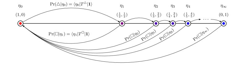
Figure 3: The states and transitions of a hidden Markov-driven iterated function system (DIFS) discussed in Section VII.1 embedded in the 1-simplex. In this case, the set of states $\bm{\mathcal{R}}$ is countable, which each subsequent application of $f^{(\triangle)}$ bringing $\eta$ nearer to $(0,1)$, which is reached only after observing infinitely many $\triangle$s. The countable nature of the state set arises from the the fact that one of the mapping functions is a constant: $f^{(\square)}=(1,0)$.

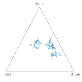
(a) Set of states generated by the “delta” DIFS.

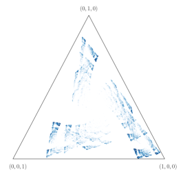
(b) Set of states generated by the “Nemo” DIFS.

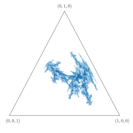
(c) Set of states generated by the “gamma” DIFS.

Figure 4: Hidden Markov driven iterated function system (DIFS) may generate state sets with a wide variety of structures, many fractal in nature. Each subplot displays $10^{5}$ states of a different DIFS. The DIFSs themselves are specified in Appendix A.

DIFS states are predictive in the sense that they are functions of the prior sequences of observables (pasts) and lead to the correct future distribution conditioned on the pasts. Consider an infinitely-long past that, in the present, has induced some state $\eta$. It is not guaranteed that this infinitely-long past induce a unique state, but it is the case that any state induced by this past must have the same conditional future distribution. Indeed, for task of prediction, knowing the previous state is as good as knowing the infinite past: $\Pr({X}_{0:\ell}|\mathcal{R}_{0}=\eta)=\Pr({X}_{0:\ell}|{X}_{-\infty:0})$ for all $\ell\in\mathbf{N}^{+}$.

Therefore, the DIFS is a predictive model of the given process $\mathcal{P}$. Contrast this to it being merely a generative model that produces all and only the sequences in a process, but whose states need not be predictive. Note that predictive models are generative.

Borrowing from the language of automata theory, we refer to the set of states $\bm{\mathcal{R}}$ plus its transition dynamic—$\Pr({x}_{t}|\eta_{t})$ and $\Pr(\eta_{t+1}|\eta_{t},{x}_{t})$—as a state machine or, simply machine that optimally predicts $\mathcal{P}$. When we force each infinitely long past to induce a unique state, we produce a canonical predictive model that is unique: a process’ $\epsilon$-machine [10].

Definition 2.

An $\epsilon$-machine is a DIFS with probabilistically distinct states: For each pair of distinct states $\eta,\zeta\in\bm{\mathcal{R}}$ there exists a finite word $w={x}_{0:\ell-1}$ such that:

$$\Pr({X}_{0:\ell}=w|\mathcal{R}_{0}=\eta)\not=\Pr({X}_{0:\ell}=w|\mathcal{R}_{0}=\zeta)~{}.$$

A process’ $\epsilon$-machine is its optimally-predictive, minimal model, in the sense that the set $\bm{\mathcal{R}}$ of predictive states is minimal compared to all its other predictive models. By capturing a process’ structure and not merely being predictive, an $\epsilon$-machine’s states are called causal states. Unless otherwise noted, we assume that all DIFS discussed here are $\epsilon$-machines.

Calculating the Shannon entropy rate for a process generated by an DIFS was the focus of our first analysis of DIFSs [11]. Due to the associated process’ ergodicity, shown there, $h_{\mu}$ may be written:

$$\widehat{h_{\mu}}^{B}=-\lim_{\ell\to\infty}\frac{1}{\ell}\sum_{t=0}^{\ell}\sum_{{x}\in\mathcal{A}}\Pr({x}|\eta_{\ell})\log_{2}\Pr({x}|\eta_{\ell})~{}.$$ (6)

This tracks the uncertainty in the next symbol ${x}$ given our current causal state $\eta_{t}$, averaged over the Blackwell measure; hence the superscript $B$. It quantifies the intrinsic randomness of the process $\mathcal{P}$.

V Statistical Complexity Dimension

Images of the self-similar DIFSs state sets $\bm{\mathcal{R}}$ (as in Fig. 4) are evocative and lead naturally to questions about how $\bm{\mathcal{R}}$’s geometric properties relate to intrinsic properties of the underlying process $\mathcal{P}$. To answer this, we say that a process’ memory is the information required to specify its $\epsilon$-machine states, i.e., the minimal amount of information needed to predict $\mathcal{P}$. This may be measured either in terms of the cardinality $|\bm{\mathcal{R}}|$ of causal states or the amount of historical Shannon entropy they store—that is, the statistical complexity $C_{\mu}$.

Definition 3.

A process’ statistical complexity is the Shannon entropy stored in its $\epsilon$-machine’s causal states:

$$C_{\mu}= \operatorname{H}[\Pr(\bm{\mathcal{R}})]$$

$$= -\sum_{\eta\in\bm{\mathcal{R}}}p(\eta)\log_{2}p(\eta)~{}.$$ (7)

From the definitions above, a process’ $\epsilon$-machine is its smallest predictive model, in the sense that both |$\bm{\mathcal{R}}|$ and $C_{\mu}$ are minimized by a process’ $\epsilon$-machine, compared to all other predictive models. Due to the $\epsilon$-machine’s unique minimality, we identify the $\epsilon$-machine’s $C_{\mu}$ as the process’ memory.

However, when the set of causal states $\bm{\mathcal{R}}$ is infinite, the statistical complexity may diverge. In this case, $C_{\mu}$ is no longer an appropriate complexity measure to distinguish processes. Despite this, a need remains: It is clear that processes with infinite state sets differ significantly in internal structure, as shown in Fig. 4. In this case, we turn to the statistical complexity dimension, defined as the rate of divergence of the statistical complexity, to serve as a measure of structural complexity. This leaves us with an abiding question, though, What does it mean that a finitely-specified process’ state information (memory) diverges?

V.1 Dimension and Causal State Divergence

A set’s dimension, construed most broadly, gives the rate at which a chosen size-metric diverges with the scale at which the set is observed [24, 25, 26, 27, 28]. Fractional dimensions, in particular, are useful to probe the “size” of sets when cardinality alone is not informative. “Fractal dimension”, said in isolation, is often taken to refer to the box-counting or Minkowski-Bouligand dimension. The following, though, determines the information dimension—a dimension that accounts for the scaling of a measure on a fractional dimension set. In this case, our measure of interest is the Blackwell measure $\mu_{B}$ over our causal states $\bm{\mathcal{R}}$.

Consider the state set $\bm{\mathcal{R}}$ on the $(N-1)$-simplex for an DIFS that generates a process $\mathcal{P}$. Coarse-grain the $N$-simplex with evenly-spaced subsimplex cells of side length $\epsilon$. Let $\mathcal{F}(\epsilon)$ be the set of cells that encompass at least one state. Now, let each cell in $\mathcal{F}(\epsilon)$ itself be a (coarse-grained) state and approximate the $\epsilon$-machine dynamic by grouping all transitions to and from states encompassed by the same cell. This results in a finite-state Markov chain that generates an approximation of the original process $\mathcal{P}$ and has a stationary distribution $\mu(\mathcal{F}(\epsilon))$. Then $\mu_{B}(\bm{\mathcal{R}})$’s information dimension is:

$$d_{1}(\mu_{B}(\bm{\mathcal{R}})) =\lim_{\epsilon\to 0}\frac{H_{\mu}[\mathcal{F}(\epsilon)]}{\log\epsilon}~{},$$ (8)

where $H_{\mu}[\mathcal{F}(\epsilon)]=-\sum_{C_{i}\in\mathcal{F}(\epsilon)}\mu(C_{i})\log\mu(C_{i})$ is the Shannon entropy over the set $\mathcal{F}(\epsilon)$ of cells that cover attractor $\bm{\mathcal{R}}$ with respect to $\mu$.

Rearranging Eq. 8 shows that the state entropy of the finite-state approximation scales logarithmically with $\bm{\mathcal{R}}$’s information dimension with respect to the Blackwell measure:

$$H_{\mu}[\mathcal{F}]\sim d_{1}(\mu_{B})\cdot\log\epsilon~{}.$$ (9)

Applied to a process $\mathcal{P}$’s $\epsilon$-machine, $d_{1}$ describes the divergence rate of statistical complexity $C_{\mu}$:

$$C_{\mu}(\epsilon)\sim d_{\mu}\cdot\log\epsilon~{}.$$ (10)

In this way, we refer to the $\epsilon$-machine’s information dimension $d_{1}(\mu_{B})$ as $\mathcal{P}$’s statistical complexity dimension $d_{\mu}$.

V.2 Determining Statistical Complexity Dimension

Directly calculating the statistical complexity dimension using Eq. 8 is nontrivial, as it often requires estimating a fractal measure. Fortunately, as two previous works discussed and as we now show, the intractability can be circumvented by leveraging the process’s associated generating dynamical system—the DIFS—to calculate $d_{\mu}$ [11, 12].

For a dynamical system, the spectrum of Lyapunov characteristic exponents $\Gamma=\{\lambda_{1},\ldots,\lambda_{N}:\lambda_{i}\geq\lambda_{i+1}\}$ [29, 30] measures expansion and contraction as the average local growth or decay rate, respectively, of orbit perturbations. The result is a list of rates that indicate long-term orbit instability ($\lambda_{i}>0)$ and orbit stability ($\lambda_{i}<0)$ in complementary directions.

Consider covering an attractor generated by a dynamical system $f$ with hypercubes of side length $\epsilon$. After applying $f$ to a hypercube $k$ times, the side lengths are approximately $\epsilon e^{\lambda_{1}k},\epsilon e^{\lambda_{2}k},\dots$, assuming that the hypercube orientation is chosen appropriately. This property allows combining the $\Gamma$ into a expression approximating the growth rate of hypercubes needed to cover the attractor, as $\epsilon\to 0$. In turn, this implies a natural relationship between the $\Gamma$ and dimensional quantities, such as Eq. 8. In point of fact, the Lyapunov dimension [31] has been conjectured to be equivalent to the information dimension for “typical systems” $f$.

Our previous work showed how to calculate $\Gamma$ for DIFSs [12]. However, since DIFSs are random dynamical systems, additional orbit expansion arises from the stochastic selection of the maps $f^{({x})}$. Indeed, for DIFSs, since the maps are contractive all expansion arises from this stochastic choice, which is measured by the Shannon entropy rate $h_{\mu}$ of the generated process $\mathcal{P}$. That is to say, for DIFSs, $\lambda_{i}<0$ for all $i$ while $h_{\mu}$ monitors the expansive exponent.

(a)

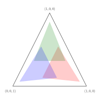
(b)

Figure 5: Overlap problem on the $2$-simplex $\Delta^{2}$: Two distinct DIFSs (given in Appendix A) are considered, each with three mapping functions. Images of the mapping functions over the entire simplex are depicted as regions in red, blue, and green. (a) Images of the mapping functions $f^{(\triangle)}$,$f^{(\square)}$, and $f^{(\circ)}$ do not overlap—every possible state has a unique pre-image. (b) Images of the mapping functions coincide: there exist $\eta_{1},\eta_{2}\in\Delta^{2}$ such that $f^{{}^{\prime}(\triangle)}(\eta_{1})=f^{{}^{\prime}(\square)}(\eta_{2})=\eta_{3}$. This case is an overlapping DIFS.

With this in mind, we adapt the Lyapunov dimension expression to DIFSs as follows:

$$\widetilde{d_{\Gamma}}=\left\{\begin{aligned} &k+\frac{\Lambda(k)+h_{\mu}}{|\lambda_{k+1}|},&-\Lambda(N)>h_{\mu}\\ &N~{},&-\Lambda(N)\leq h_{\mu}\end{aligned}\right.~{},$$ (11)

where we introduce the Lyapunov spectrum partial sum $\Lambda(m)=\sum_{i=1}^{m}\lambda_{i}$ and $k=0,1,2,\ldots,N-1$ is the largest index for which $-\Lambda(k)<h_{\mu}$. Note $\Lambda(m)<0,m=1,2,\ldots,N$ and we take $\Lambda(0)=0$. Readers familiar with the Lyapunov dimension should take care as we have re-indexed from the traditional presentation of $d_{\Gamma}$ for readability.

Under specific technical conditions, $d_{\Gamma}$ is exactly the information dimension of the DIFS’s attractor: $d_{\Gamma}=d_{\mu}$ [32]. Generally, relaxing the conditions, $\widetilde{d_{\Gamma}}$ only upper bounds the statistical complexity dimension:

$$\widetilde{d_{\Gamma}}\geq d_{\mu}~{}.$$ (12)

The extent to which the bound is not saturated is in large part determined by the open set condition, which we now discuss. We, then, turn to solve the associated “overlap problem”. This leads to an exact expression for DIFS attractor information dimension $d_{\mu}$.

Figure 6: Sources of ambiguity rate depicted in state machines: (A) $H[{X}_{0}|\mathcal{R}_{0},\mathcal{R}_{1}]>0$—Previous state $\mathcal{R}_{0}$ is mapped to the next state $\mathcal{R}_{1}$ by two distinct symbols. This occurs when two symbols have identical mapping functions. (B) $I[{X}_{0};\mathcal{R}_{0}|\mathcal{R}_{1}]>0$—Two distinct previous states $\mathcal{R}_{0}$ map to the same next state by distinct symbols, due to overlapping mapping functions. (C) $H[\mathcal{R}_{0}|{X}_{0},\mathcal{R}_{1}]>0$—Two distinct previous states $\mathcal{R}_{0}$ map to the same next state by the same symbol. This occurs when a mapping function is noninvertible.

V.3 The Overlap Problem

The overlap problem is a long-standing concern for iterated function systems that arises from coinciding ranges of the symbol-labeled mapping functions $f^{({x})}$. Figure 5 illustrates the issue and Ref. [12] characterized it. Specifically, to quantitatively count system orbits we must properly monitor orbit divergence and convergence. This then requires distinguishing between iterated function systems that meet the open set condition (OSC) and those that do not.

Definition 4.

An iterated function system with mapping functions $f^{({x})}:\Delta^{N}\to\Delta^{N}$ satisfies the open set condition (OSC) if there exists an open set $U\in\Delta^{N}$ such that for all $\eta,\zeta\in\Delta^{N}$:

$$f^{\eta}(U)\cap f^{\zeta}(U)=\emptyset~{},$$

where $\eta\neq\zeta$. IFSs that meet the OSC are nonoverlapping.

When the OSC is not met, the inequality in the $d_{\mu}$ bound Eq. 12 becomes strict. This is a consequence of using $h_{\mu}$ as our measure of state space expansion in Eq. 11. The Shannon entropy rate tracks the uncertainty in the next symbol ${x}$ given our current causal state $\eta_{t}$, averaged over the Blackwell measure. From a dynamical systems point of view, we identify this as the typical growth rate of orbits (words) in symbol space.

When the OSC is met, the Shannon entropy rate also measures the typical growth rate of orbits in the $(N-1)$-simplex. Observing ${x}$, current state $\eta_{t}$ transitions to the next state $\eta_{t+1}$ via application of the mapping function $\eta_{t+1}=f^{({x})}(\eta_{t})$. By the OSC, this is guaranteed to be a distinct new state—thus state sequences grow at the same rate as words do. Then, we may use $h_{\mu}$ to measure expansion of the state space.

However, when the OSC is not met, it is possible for two distinct states $\eta_{t},\zeta_{t}\in\Delta$ to map to the same next state on different symbols, by occupying the “overlapping region”, as depicted in Fig. 5. In this case, $\eta_{t+1}=\zeta_{t+1}$ has no unique pre-image. This introduces ambiguity about the past, given knowledge of the current state. As a consequence, the Shannon entropy rate, which tracks uncertainty in symbol space, implies a larger expansion in state space than is actually occurring. This indicates the need to correct $h_{\mu}$, when determining $d_{\mu}$.

VI ambiguity rate

The following introduces the ambiguity rate to correct $\widetilde{d_{\Gamma}}$ of Eq. 11 from overcounting orbits. Since the problem at hand is an overestimation in uncertainty in our state space, we must identify and quantify mechanisms of state uncertainty reduction when the OSC is not met. Consider that when the OSC is met, every state $\eta_{t}$ has a unique pre-image $\eta_{t-1}$ that can only be reached via a single, specific observed symbol. When the OSC is not met, for a subset of $\eta\in\bm{\mathcal{R}}$ there is uncertainty about the previous state, the previous symbol, or both. Quantifying this ambiguity about the past is the goal in constructing the ambiguity rate $h_{a}$.

Intuitively, it would seem that generating uncertainty in reverse time is equivalent to reduction of uncertainty in forward time. The following shows that this is the case and that the ambiguity rate is the necessary correction to the DIFS dimension formula Eq. 11.

VI.1 Sources of State Uncertainty Reduction

For $\epsilon$-machines represented as DIFSs, there are three distinct mechanisms that contribute to the ambiguity rate, as depicted in Fig. 6.

The first is identical mapping functions, depicted in Fig. 6 (a). When for ${x},{x}^{\prime}\in\mathcal{A}$, $f^{({x})}(\eta)=f^{({x}^{\prime})}(\eta)$ for all $\eta\in\bm{\mathcal{R}}$, we say that ${x}$ and ${x}^{\prime}$ have identical mapping functions. In this case, the distinction between ${x}$ and ${x}^{\prime}$ is not reflected in state sequences and produces ambiguity in the symbol sequence. We quantify this as the Shannon entropy $H[{X}_{t}|\mathcal{R}_{t},\mathcal{R}_{t+1}]$ in our current symbol, conditioned on the previous state and the next state.

The second is overlapping mapping functions, which motivated this investigation and already have been defined. Their impact on the state machine is shown in Fig. 6 (b). In this case, two distinct symbols ${x},{x}^{\prime}\in\mathcal{A}$ map two distinct states $\eta,\zeta\in\bm{\mathcal{R}}$ to the same next state. Although the previous state affects the probability distribution over the observed symbol, the next state “forgets” that distinction. This is quantified by the mutual information $I[{X}_{t};\mathcal{R}_{t}|\mathcal{R}_{t+1}]$ shared by the current symbol and the previous state, conditioned on the next state.

Finally, there is noninvertibility in the mapping functions. If a single function maps distinct states $\eta,\zeta\in\bm{\mathcal{R}}$ to the same next state, the pasts that led to $\eta$ and $\zeta$ can no longer be distinguished. Figure 6 (c) shows this in general. However, it may also be observed in $f^{(\square)}$ from Fig. 3, which maps every state to $\eta_{0}=(1,0)$. The reduction via this mechanism is measured by the Shannon entropy $H[\mathcal{R}_{t}|{X}_{t},\mathcal{R}_{t+1}]$ in the previous state, given our next state and current symbol.

Combining these three sources of uncertainty reduction defines the ambiguity rate:

$$h_{a}= \>H[{X}_{t}|\mathcal{R}_{t},\mathcal{R}_{t+1}]+I[{X}_{t};\mathcal{R}_{t}|\mathcal{R}_{t+1}]$$

$$\>\>\>\>+H[\mathcal{R}_{t}|{X}_{t},\mathcal{R}_{t+1}]$$

$$= \>H[{X}_{t},\mathcal{R}_{t}|\mathcal{R}_{t+1}]~{}.$$ (13)

This can be rewritten as a integral over $\bm{\mathcal{R}}$:

$$h_{a}=-\int_{\eta\in\bm{\mathcal{R}}}\!\!\!\text{d}\mu_{B}(\eta)\!\!\!\!\!\!\!\!\!\sum_{\begin{subarray}{c}{x}\in\mathcal{A},\\ \zeta\in(f^{({x})})^{-1}(\eta)\end{subarray}}\!\!\!\!\!\!\!\!\!\Pr({x},\zeta|\eta)\log_{2}\Pr({x},\zeta|\eta).$$ (14)

In this, we must be careful about the pre-images of $\eta$, due to the possibility of noninvertible mapping functions. The probability distribution inside the summation is given by the relationship:

$$\Pr({X}_{0}={x},\mathcal{R}_{0}=\zeta |\mathcal{R}_{1}=\eta)=$$

$$\frac{\mu_{B}(\mathcal{R}_{0}=\zeta)}{\mu_{B}(\mathcal{R}_{1}=\eta)} \times\Pr({X}_{0}={x}|\mathcal{R}_{0}=\zeta)~{}.$$ (15)

Calculating this distribution requires calculating or estimating the Blackwell measure, which may be nontrivial. Section VII discusses this in greater depth.

VI.2 Correcting $d_{\mu}$

The information-theoretic decomposition of ambiguity rate facilitates combining $h_{a}$ and $h_{\mu}$. Recall that for prediction, the states of a predictive model are equivalent to knowledge of the infinite past. Due to this, the Shannon entropy rate may be written $H[{X}_{t}|\mathcal{R}_{t}]$. Combining this with the ambiguity rate gives:

$$h_{\mu}-h_{a} =H[{X}_{t}|\mathcal{R}_{t}]-H[{X}_{t},\mathcal{R}_{t}|\mathcal{R}_{t+1}]$$

$$=H[\mathcal{R}_{t+1}|\mathcal{R}_{t},{X}_{t}]+H[\mathcal{R}_{t+1}]-H[\mathcal{R}_{t}]$$

$$=\Delta H[\mathcal{R}_{t}]~{}.$$

Moving to the third line—that is, noting that the first term vanishes—called on the fact that the symbol and state transitions are defined by functions. So, the difference between the Shannon entropy rate and the ambiguity rate is the growth rate of the causal state set $\mathcal{R}$.

Recall that the information dimension, as defined in Eq. 8, compares the average growth of occupied cells $\mathcal{F}$—taking into account the measure over those cells—as the cell size $\epsilon$ shrinks. To adhere to the main development, here we will not walk through the heuristic for how a dimensional quantity is determined from the $\Gamma$. (Though, this is briefly discussed in Section V.2.) Nonetheless, we will show how the relationship between $d_{1}$, $h_{\mu}-h_{a}$, and $\Gamma$ is intuitive for DIFSs in one dimension.

When the DIFS states lie in the 1-simplex, $\Gamma$ consists of only one exponent $\lambda_{1}<0$, which is the weighted average of the Lyapunov exponents of each map:

$$\lambda_{1}=\int\sum_{{x}}p^{({x})}(\eta)\log\left|\frac{df^{({x})}(\eta)}{d\eta}\right|d\mu~{},$$

where $\mu$ is the Blackwell measure.

Now, consider a line segment in $\Delta^{1}$ of length $\epsilon$. Mapping this line forward $k$ times by the DIFS produces, averaging over several iterations of this action, $2^{(h_{\mu}-h_{a})k}$ new lines of length $\epsilon e^{\lambda_{1}k}<\epsilon$. (Note that the use of base-two for Shannon entropy rather than base $e$ follows convention; retained here for familiarity. When numerically estimating $d_{\mu}$, we recommend a consistent base be chosen for $h_{\mu}$, $h_{a}$, and the $\Gamma$.) The logarithmic ratio of the growth rate of lines (as averaged over the Blackwell measure) compared to the shrinking of these lines is the simple ratio:

$$d_{\mu} =-\frac{h_{\mu}-h_{a}}{\lambda_{1}}~{}.$$

This, of course, is exactly the definition of the information dimension Eq. 8 and is, assuming the DIFS is an $\epsilon$-machine, the statistical complexity dimension $d_{\mu}$.

For higher-dimensional DIFSs, we conjecture that the ambiguity rate is the adjustment to the IFS Lyapunov dimension formula that gives the information dimension:

$$\widetilde{d_{\mu}}=\left\{\begin{aligned} &k+\frac{\Lambda(k)+h_{\mu}-h_{a}}{|\lambda_{k+1}|},&-\Lambda(N)>h_{\mu}-h_{a}\\ &N~{},&-\Lambda(N)\leq h_{\mu}-h_{a}\end{aligned}\right.,$$ (16)

where as in Eq. 11, $\Lambda(m)$ is the Lyapunov spectrum partial sum $\Lambda(m)=\sum_{i=1}^{m}\lambda_{i}$ and $k=0,1,2,\ldots,N-1$ is the largest index for which $-\Lambda(k)<h_{\mu}-h_{a}$.

VI.3 Interpreting Ambiguity Rate

Up to this point, we motivated ambiguity rate as correcting over counting in the DIFS statistical complexity dimension $d_{\mu}$. It is worth discussing the quantity in more depth.

On the one hand, note that when $h_{\mu}-h_{a}=0$, the causal-state process is stationary and $C_{\mu}$ time-independent: $\Delta H[\mathcal{R}_{t}]=0$. This occurs for finite-state DIFSs, as well as many with countably-infinite states; see Section VII.1. When this occurs, applying Eq. 16 returns a vanishing statistical complexity dimension $d_{\mu}=0$, as expected.

On the other hand, when ambiguity rate vanishes, $C_{\mu}$ grows at the Shannon entropy rate: $\Delta H[\mathcal{R}_{t}]=h_{\mu}$. This occurs when there are no identical maps, no overlap, and no noninvertibility in the mapping functions. In short, $h_{a}=0$ when the causal-state process is “perfectly self-similar” and every new observed symbol produces a new, distinct state.

With this in mind, we can use the ambiguity rate, and specifically $h_{\mu}-h_{a}$, to describe the stationarity of the model’s internal state process. The state set is time independent. When $h_{a}>0$, however, to optimally predict the process $\mathcal{P}$ requires a nonstationary model (temporally-growing state set $\bm{\mathcal{R}}$), even though $\mathcal{P}$ is itself stationary. This is a consequence of modeling “out of class”. That is, predicting a perfectly self-similar $\mathcal{P}$ requires differentiating every possible infinite past. This is only possible with a DIFS by storing new states at the rate new pasts are being created. (Moving to a more powerful model class by, say, imbuing our states with counters or stacks, may make it possible to model $\mathcal{P}$ with a stationary model.)

This perspective naturally leads to another that probes the efficacy of the causal-state mapping. Considering the space of all possible infinite pasts $\overleftarrow{{X}}$, the causal-state mapping $f_{\epsilon}(\overleftarrow{{X}})\rightarrowtail\bm{\mathcal{R}}$ is defined such that:

$$f_{\epsilon}(\overleftarrow{{X}}=\overleftarrow{{x}})=f_{\epsilon}(\overleftarrow{{X}}=\overleftarrow{{x}^{\prime}})=\eta_{i}~{},$$

if $\Pr({X}_{0:\ell}|\overleftarrow{{X}}=\overleftarrow{{x}})=\Pr({X}_{0:\ell}|\overleftarrow{{X}}=\overleftarrow{{x}^{\prime}})$ for all $\ell\in\mathbf{N}^{+}$. When the process is perfectly self-similar, the causal-state mapping is one-to-one and $h_{a}=0$. In this case, storing the causal states is no better for prediction than simply tracking the space of all pasts. (Although the causal-state set $\bm{\mathcal{R}}$ is still informative in characterizing how we might approximate the process with a finite state machine [33].) The number of pasts each state “contains” is stationary and given by $2^{h_{a}}=1$.

In general, for a stationary process $\mathcal{P}$, the average number of pasts contained by a given causal state grows at the rate $2^{h_{a}}$. When the process has a stationary state set, the number of pasts each state contains must necessarily grow at the rate new pasts are being generated, and so $2^{h_{\mu}}=2^{h_{a}}$.

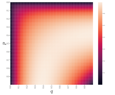
Figure 7: The entropy rate $h_{\mu}$, which in this case is equivalent to the ambiguity rate $h_{a}$, is plotted for the DIFS depicted in Fig. 3 for $p,q,\in(0,1)$.

Finally, let’s close with a short historical perspective. The development of $d_{\mu}$ was partially inspired by Shannon’s definition in the 1940s of dimension rate [4]:

$$\lambda=\lim_{\delta\to 0}\lim_{\epsilon\to 0}\lim_{T\to\infty}\frac{N(\epsilon,\delta,T)}{T\log\epsilon}~{},$$

where $N(\epsilon,\delta,T)$ is the smallest number of elements that may be chosen such that all elements of a trajectory ensemble generated over time $T$, apart from a set of measure $\delta$, are within the distance $\epsilon$ of at least one chosen trajectory. This is the minimal “number of dimensions” required to specify a member of a trajectory (or message) ensemble. Unfortunately, Shannon devotes barely a paragraph to the concept, leaving it largely unmotivated and uninterpreted.

Therefore, it appears the first modern discussion of a dimensional quantity of this nature for stochastic processes motivated the development using resource theory [33], noting that the $d_{1}$ of the causal-state set Eq. 8 characterizes the distortion rate when coarse-graining an uncountably-infinite state set. Starting from the dimensional quantity, the relationship to statistical complexity was then forged.

In this light, developing ambiguity rate and calling out its easy mathematical connection to $\Delta H[\bm{\mathcal{R}}_{t}]$ flips this motivation. The quantity $h_{\mu}-h_{a}$ can be defined purely in terms of $\mathcal{P}$ and has an intuitive relationship to the causal-state mapping. The dimensional quantity $d_{\mu}$ naturally falls out when we compare this rate of model-state growth to the dynamics of the causal states in the mixed-state simplex. Therefore, we may motivate $d_{\mu}$ not as only a resource-theoretic tool for finitizing infinitely-complex state machines, but also as an intrinsic measurement of a process’ structural complexity.

VII Examples

We now consider two examples. The first is a parametrized discrete-time renewal process that has a countably-infinite state space for all parameters. This allows us to explicitly write down the Blackwell measure and calculate ambiguity rate exactly using Eq. 14. The second is a parametrized machine with three maps, which has an uncountably-infinite state space for nearly all parameters. Calculating the ambiguity rate in this case requires us to approximate the Blackwell measure using Ulam’s method.

Figure 8: One-dimensional attractor for DIFS given in Section VII.2 with $x=0.25$ and horizontally varying $\alpha\in(0,1)$. State set $\eta\in\bm{\mathcal{R}}$ plotted (red, blue, green) on top of the images of the mapping functions $\left\{f^{(\triangle)},f^{(\square)},f^{(\circ)}\right\}$ applied to $\bm{\mathcal{R}}$. For $\alpha\in(0.07,0.78)$, there is overlap in the images of the maps.

VII.1 Example: Discrete-Time Renewal Process

The DIFS depicted in Fig. 3 has the alphabet $\mathcal{A}=\{\triangle,\square\}$ and the substochastic matrices:

$$T^{\triangle}=\begin{pmatrix}1-q&q\\ 0&1-p\end{pmatrix}~{}\text{and}~{}T^{\square}=\begin{pmatrix}0&0\\ p&0\end{pmatrix}~{},$$ (17)

where $p=q=\frac{1}{2}$. For the general case where $p,q\in(0,1)$ are left unspecified, we have the probability function set:

$$p^{(\triangle)}(\eta) =1-\langle\eta|\delta_{2}\rangle p~{},$$

$$p^{(\square)}(\eta) =\langle\eta|\delta_{2}\rangle p~{},$$

and the mapping function set:

$$f^{(\triangle)}(\eta) =\left(\frac{\langle\eta|\delta_{1}\rangle(1-q)}{1-\langle\eta|\delta_{2}\rangle p},\frac{\langle\eta|\delta_{1}\rangle q+\langle\eta|\delta_{2}\rangle(1-p)}{1-\langle\eta|\delta_{2}\rangle p}\right)~{},$$

$$f^{(\square)}(\eta) =\left(1,0\right)~{}.$$

Since $\bm{\mathcal{R}}$ is countable, we may write down the state set $\bm{\mathcal{R}}$ as a sequence:

$$\eta_{n}=\left[\frac{(p-q)(1-q)^{n}}{p(1-q)^{n}-q(1-p)^{n}},\frac{q(1-q)^{n}-q(1-p)^{n}}{p(1-q)^{n}-q(1-p)^{n}}\right]~{},$$

where $n$ is the number of $\triangle$s seen since the last $\square$ and $p\neq q$. This simple structure allows us to give the Blackwell measure explicitly:

$$\mu_{B}(n)=\frac{p(1-q)^{n}-q(1-p)^{n}}{p-q}\times\frac{pq}{p+q}~{},$$

where $\mu_{B}(n)$ is the asymptotic invariant measure over the state induced after seeing $n$ $\triangle$s since the last $\square$.

With the Blackwell measure in hand, the entropy rate can be explicitly calculated as the infinite sum:

$$h_{\mu}= \>\sum_{n=1}^{\infty}\mu_{n}H[{X}_{n}|\mathcal{R}_{n}=\eta_{n}]$$

$$= \>-\sum_{n=1}^{\infty}\mu_{n}\Big{(}p^{(\triangle)}(\eta_{n})\log_{2}p^{(\triangle)}(\eta_{n})$$

$$\qquad\qquad\quad+p^{(\square)}(\eta_{n})\log_{2}p^{(\square)}(\eta_{n})\Big{)}~{}.$$

Figure 7 plots $h_{\mu}$ for $p,q\in(0,1)$. In calculating $h_{\mu}$, there is a contribution from every state except the first—$\eta_{0}$—since the first state transitions to the second with probability one and there is no branching uncertainty. Every other state transitions on a coin flip of a determined bias between $(\triangle,\square)$, generating uncertainty with each transition.

In contrast to how $h_{\mu}$ averages over all mixed states, ambiguity rate accumulates in only one state—$\eta_{0}$. From Fig. 3, we see that $H[{x}_{n},\eta_{n}|\eta_{n+1}]=0$ for all $n$ other than $n=0$. That is, each state $\eta_{n}$ is only accessed via the prior state $\eta_{n-1}$, except for $\eta_{0}$, which may be accessed from every other state. So, ambiguity in the past can only be introduced by visiting $\eta_{0}$. Since these transitions only occur on a $\square$, we must find the probability distribution $\Pr({X}_{0}=\square,\mathcal{R}_{0}=\eta_{n}|\mathcal{R}_{1}=\eta_{0})$.

Applying Eq. 14 and Eq. 15, we explicitly write down the ambiguity rate as:

$$h_{a}=\mu_{0}\sum_{n=1}^{\infty}\left(\frac{\mu_{n}}{\mu_{0}}p^{(\square)}(\eta_{n})\right)\log_{2}\left(\frac{\mu_{n}}{\mu_{0}}p^{(\square)}(\eta_{n})\right)~{}.$$

Both $h_{\mu}$ and $h_{a}$ are infinite summations, but when calculating the ambiguity rate, the sum refers to calculating a single Shannon entropy over the infinite, discrete distribution representing the probability distribution over prior states when arriving in $\eta_{0}$.

Since the state space does not grow—$\Delta H[\bm{\mathcal{R}}_{t}]=0$—the entropy rate $h_{\mu}=h_{a}$ as $n\to\infty$. Therefore, $d_{\mu}$ vanishes for all values of $p$ and $q$. This will always be the case for finite-state DIFSs and, in general, for those with countable state spaces.

Figure 9: Calculating entropies and dimensions for the DIFS given in Section VII.2 with $\alpha\in(0,1)$, and $x=0.25$: (Top) The entropy rate $h_{\mu}$, the ambiguity rate $h_{a}$, and $h_{\mu}-h_{a}$. (Bottom) Comparing $h_{\mu}/\lambda_{1}$ to $d_{\mu}=(h_{\mu}-h_{a})/\lambda_{1}$: The latter smoothly departs from the former and is approximately $1$ for much of the overlap region, except where it discontinuously jumps to zero at $\alpha=1/3$.

VII.2 Example: 1-D Ambiguity Rate

Now, let’s turn to the more general case, those DIFSs with uncountably-infinite state spaces. For the moment we restrict to one-dimensional DIFSs, so that the states lie in the $1$-simplex. Consider a DIFS with the alphabet $\mathcal{A}=\left\{\triangle,\square,\circ\right\}$ and the associated substochastic matrices:

$$T^{\triangle} =\begin{pmatrix}\alpha y&\beta x\\ \alpha x&\beta y\end{pmatrix},~{}T^{\square}=\begin{pmatrix}\beta y&\beta x\\ \beta x&\beta y\end{pmatrix},~{}\text{and}$$

$$T^{\circ} =\begin{pmatrix}\beta y&\alpha x\\ \beta x&\alpha y\end{pmatrix}~{},$$ (18)

with $\alpha=1-2\beta,\alpha\in(0,1)$, and $x=1-y,x\in(0,1)$.

Figure 8 depicts all of the DIFSs for the slice of the parameter space where $x=0.25$. The vertical axis is the $1$-simplex and each vertical slice plots the state space $\bm{\mathcal{R}}(\alpha)$ at the appropriate value of $\alpha$, given on the horizontal axis. Additionally, the images of the functions $\left\{f^{(\triangle)}(\bm{\mathcal{R}}),f^{(\square)}(\bm{\mathcal{R}}),f^{(\circ)}(\bm{\mathcal{R}})\right\}$ are shaded in red, blue, and green, respectively.

At $\alpha=1/3$, the mixed state set $\bm{\mathcal{R}}$ contracts to a finite set, and $h_{\mu}$ must equal to $h_{a}$, making $d_{\mu}=0$. At this point in parameter space, the state set consists of only one state; $\bm{\mathcal{R}}(\alpha=1/3)=\{(1/2,1/2)\}$. At every other value of $\alpha$, $h_{a}<h_{\mu}$. There is overlap in the images of the maps for, approximately, $\alpha\in(0.07,0.78)$. In this regime, $h_{a}>0$.

To calculate the ambiguity rate and therefore the statistical complexity dimension $d_{\mu}$ we use a modified Ulam’s method to approximate the Blackwell measure and then approximate the integral equation Eq. 14. This method is not the only way to find the ambiguity rate, but does have several advantages, including speed and the ability to control the accuracy of our approximation. This method is discussed in depth in Appendix B.

The top plot in Fig. 9 gives the entropy rate, ambiguity rate, and $h_{\mu}-h_{a}$ for the DIFSs pictured in Fig. 8. As $\alpha$ is increased, $h_{a}$ smoothly increases from zero as overlap begins to occur. It approaches $\approx 0.6$ around $\alpha=1/3$, but is discontinuously equal to zero at this point. The reason for this is an instantaneous equality in the fixed points of the mapping functions, causing the state space to collapse. As $\alpha$ increases to $1$, $h_{a}$ smoothly decreases back to zero. The roughness seen in the plot is due to numerical precision, as explained in Appendix B.

For a large portion of the overlap region, $d_{\Gamma}$ saturates at 1.0. The bottom plot in Fig. 9 instead depicts $h_{\mu}/\lambda_{1}$ to show how this quantity smoothly changes across parameter space, reaching a maximum around $\alpha\approx 1.6$. By way of comparison, $d_{\mu}=(h_{\mu}-h_{a})/\lambda_{1}$ smoothly departs from the Lyapunov dimension when overlap begins and, instead, asymptotes from below to the $\dim=1.0$ line for much of the overlap region. Again, at $\alpha=1/3$ there is the discontinuous drop to $d_{\mu}=0$, followed by $d_{\mu}$ smoothly rejoining with the Lyapunov dimension as the overlap region ends.

Unsurprisingly, calculating the ambiguity rate in higher dimensions is more challenging. Although, in principle, Ulam’s method still applies and we may in principle follow the algorithm laid out in Appendix B, higher-dimensional mapping functions introduce additional error sources in the approximation. Developing an algorithm to efficiently and accurately calculate the ambiguity rate in higher dimensions is of great interest. We leave this task to future work, however, having achieved our goal of introducing a method to estimate the statistical complexity dimension.

VIII Conclusion

Stepping back from developing ambiguity rate and statistical complexity dimension, let us position the new results here in the context of our prior two works in this series [11, 12]. In the first, motivated by needing a general solution to the Shannon entropy rate for processes generated by finite-state hidden Markov chains, we showed how an optimal predictor can be constructed for any such process, at the cost of a potentially uncountably-infinite state space. To address the resulting challenge, we introduced hidden Markov-driven iterated function systems and showed that the attractor of a properly-defined DIFS is equivalent to the $\epsilon$-machine for the process generated by its substochastic matrices.

The result gave benefits beyond a finite-dimensional description of an infinite-state model. The identification allowed us to adopt several rigorous results on IFSs, including an ergodic theorem that allows us to sample the DIFS to accurately and efficiently calculate the Shannon entropy rate of the underlying process. With this, our original goal was completed.

However, identifying these $\epsilon$-machines as IFSs allowed us to show that the dimension of the mixed state set, a quantity well studied for IFSs, is a structural complexity measure for stochastic processes. The second prequel Ref. [12] then introduced the statistical complexity dimension—the DIFS attractor information dimension. A long-standing conjecture in dynamical systems theory states that the Lyapunov dimension, a dimensional quantity calculated using a system’s Lyapunov spectrum, is equivalent to the information dimension. We showed that for many DIFSs this is indeed the case, connecting the information dimension of the $\epsilon$-machine’s state space to the $\epsilon$-machine’s statistical complexity dimension—the rate of divergence of the statistical complexity. This related a DIFS’s dynamics to the information-theoretic properties of the underlying process. Additionally, it gave a new and meaningful measure of structural complexity—one that differentiates between stochastic processes with divergent state spaces.

That was not the end of the story, since calculating $d_{\mu}$ is difficult due to long-standing challenges in the field of IFS dimension theory. In particular, the overlap problem posed a significant hurdle—restricting the preceding results to only nonoverlapping IFSs. This limited analyses to the class of stochastic processes with one-to-one past-to-causal state mappings. In one sense, these processes are the most complex but exhibit structure that is the least interesting. That is, for processes generated by these DIFSs one simply stores every past to build an optimally-predictive model.

This state of affairs led directly to the present development and to introducing the ambiguity rate. The latter allows smoothly varying between $\epsilon$-machines with countable state spaces ($h_{a}=h_{\mu}$ and $\Delta H[\bm{\mathcal{R}}]=0$) and those with perfectly self-similar state spaces ($h_{a}=0$ and $\Delta H[\bm{\mathcal{R}}]=h_{\mu}$), including all those lying in between, with $h_{\mu}>h_{a}>0$ and $\Delta H[\bm{\mathcal{R}}]=h_{\mu}-h_{a}$. This model class is much more general, generating an exponentially larger family of stochastic processes. As such, we anticipate that this class will be of great interest and likely to lead to significant further progress in analyzing the randomness and structure generated by hidden Markov chains.

To close, we note that the structural tools and the entropy-rate method introduced by this trilogy were put to practical application in two other previous works. One diagnosed the origin of randomness and structural complexity in quantum measurement [34]. The other exactly determined the thermodynamic functioning of Maxwellian information engines [35], when there had been no previous method for this kind of detailed and accurate classification. The lesson from these applications of finite-state-generated processes is that the resulting effectively-infinite state processes are very likely generic. That said, for now we must leave to the future investigating infinite-state machines and developing the required algorithmic tools.

Supplementary Materials
Ambiguity Rate of
Hidden Markov Processes
Alexandra Jurgens and James P. Crutchfield
arXiv:2002.XXXXX

The Supplementary Materials to follow give a suite of example hidden Markov chains and discuss numerically estimating the ambiguity rate.

Appendix A Hidden Markov-Driven Iterated Function System Examples

We reproduce here the hidden Markov-driven iterated function systems (DIFS) used to create Fig. 4.

First, the delta DIFS, from Fig. 4a, is given by a three-symbol alphabet and the substochastic symbol-labeled matrices:

$$T^{\square} =\begin{pmatrix}0.112&0.355&3.901\times 10^{-2}\\ 0.434&7.685\times 10^{-2}&2.333\times 10^{-2}\\ 0.215&2.518\times 10^{-2}&0.220\end{pmatrix},$$ (S1)

$$T^{\triangle} =\begin{pmatrix}1.778\times 10^{-2}&0.113&0.220\\ 6.465\times 10^{-2}&0.272&2.413\times 10^{-2}\\ 0.400&8.697\times 10^{-3}&9.892\times 10^{-3}\end{pmatrix},~{}\text{and}~{}$$

$$T^{\circ} =\begin{pmatrix}8.312\times 10^{-2}&2.867\times 10^{-2}&3.096\times 10^{-2}\\ 4.690\times 10^{-2}&5.625\times 10^{-2}&1.807\times 10^{-3}\\ 0.114&1.095\times 10^{-3}&7.522\times 10^{-4}\end{pmatrix}~{},$$

Second, the Nemo DIFS, from Fig. 4b, is given by a two-symbol alphabet and the substochastic symbol-labeled matrices:

$$T^{\square} =\begin{pmatrix}0.409&0.0&0.091\\ 0.5&0.0&0.0\\ 0.0&0.182&0.0\end{pmatrix},~{}\text{and}~{}$$ (S2)

$$T^{\triangle} =\begin{pmatrix}0.091&0.0&0.409\\ 0.5&0.0&0.0\\ 0.0&0.818&0.0\end{pmatrix}~{},$$

Finally, the gamma DIFS, from Fig. 4c, is given by a three-symbol alphabet and the substochastic symbol-labeled matrices:

$$T^{\square} =\begin{pmatrix}2.479\times 10^{-2}&0.355&1.745\times 10^{-2}\\ 0.410&1.878\times 10^{-2}&2.388\times 10^{-4}\\ 0.204&2.472\times 10^{-3}&0.215\end{pmatrix},$$ (S3)

$$T^{\triangle} =\begin{pmatrix}1.672\times 10^{-3}&0.133&0.235\\ 3.377\times 10^{-2}&0.272&8.277\times 10^{-2}\\ 0.426&1.498\times 10^{-2}&4.286\times 10^{-3}\end{pmatrix},~{}\text{and}~{}$$

$$T^{\circ} =\begin{pmatrix}8.870\times 10^{-2}&3.059\times 10^{-2}&0.114\\ 6.918\times 10^{-2}&0.112&1.804\times 10^{-3}\\ 0.131&1.165\times 10^{-3}&8.005\times 10^{-4}\end{pmatrix}~{},$$

Due to finite numerical accuracy, reproducing the attractors using these specifications may differ slightly from Fig. 4.

The mapping images shown in Fig. 5 are produced by the following three-symbol DIFS:

$$T^{\square} =\begin{pmatrix}\alpha y&\beta x&\beta x\\ \alpha x&\beta y&\beta x\\ \alpha x&\beta x&\beta y\end{pmatrix},~{}T^{\triangle}=\begin{pmatrix}\beta y&\alpha x&\beta x\\ \beta x&\alpha y&\beta x\\ \beta x&\alpha x&\beta y\end{pmatrix},~{}\text{and}$$

$$T^{\circ} =\begin{pmatrix}\beta y&\beta x&\alpha x\\ \beta x&\beta y&\alpha x\\ \beta x&\beta x&\alpha y\end{pmatrix}~{},$$ (S4)

with $\alpha=0.63$ and $x=0.2$ for the overlapping example in Fig. 5a and $\alpha=0.6$ and $x=0.15$ for the nonoverlapping example in Fig. 5b.

Figure S1: DIFS for $x=0.25$ and $\alpha=0.5$: (Top) Blackwell Measure $\mu_{B}$ approximated by Ulam’s method with $k=400$. The two overlapping regions are overlaid and may be compared with Fig. 8. (Middle) Probability of each prior map is plotted. In nonoverlapping regions, only one prior map is possible. In the overlapping regions, there are complicated, fractal-like distributions over multiple prior maps. (Bottom) Shannon entropy over the prior map: Nonzero only in the overlapping regions.

Appendix B Numerical Approximation of Ambiguity Rate

To estimate the ambiguity rate for a DIFS lying in the $1$-simplex, we may use Ulam’s method to approximate the Blackwell measure, then compute Eq. 14. Given a partition $\{A_{1},\dots A_{k}\}$ of the simplex, define:

$$P_{ij}^{({x})}=\frac{m(f^{({x})}(A_{i})\cap A_{j})}{m(f^{({x})}(A_{i}))}\times p^{({x})}\left(\overline{A_{i}}\right)~{},$$

where $m$ is the Lebesgue measure over $\Delta$ and $\overline{A_{i}}$ is the center of a partition element. Let $P=\sum P^{({x})}$ and find the left eigenvalue $p=pP$. Then, the invariant-measure approximation is:

$$\mu_{n}(A)=\sum_{i}p_{i}\frac{m(A\cap A_{i})}{m(A_{i})}~{}.$$

For this example, let’s walk through estimating the ambiguity rate for one DIFS—setting $x=0.25$ and $\alpha=0.5$. The partition $\{A_{1},\dots A_{k}\}$ is created by dividing the $1$-simplex into $k$ boxes of equal length. The approximated Blackwell measure $\widehat{\mu_{B}}$ for the DIFS, using $k=400$, is shown in the top plot of Fig. S1. The overlay indicates the region (green) of the state space that exhibits overlap. Compare the two regions depicted in Fig. S1 to the overlap shown in Fig. 8, for the vertical slice at $\alpha=0.5$.

Note that the partition may be defined as desired. We have found that defining the partition by calculating the set of fixed points of the mapping functions $\left\{p^{{x}}:f^{({x})}(p^{{x}})=p^{{x}}\right\}$. Then, as many times as is desired, find all possible iterates of each fixed point, constructing a new set $\left\{f^{(w)}(p^{{x}}):{x}\in\mathcal{A},w\in\bigcup_{n=0}^{N}\mathcal{A}^{n}\right\}$, where $N\in\mathbb{Z}^{+}$. Removing duplicates and ordering the set gives a list of endpoints for a partition of the $1$-simplex. Increasing $N$ produces increasingly fine partitions. This method of defining partitions has advantages when calculating $h_{a}$ across parameter space as we have in Section VII.2, since the position of the fixed point iterates in the simplex are smooth functions of $\alpha$.

Regardless, once the partition is selected and $\widehat{\mu_{B}}$ is determined, we again use the partition. For each cell $A_{i}$, we find the probability distribution over the maps that could have transitioned into $A_{i}$. By applying Eq. 15 and assuming invertibility of the mapping functions gives:

$$\Pr({X}_{0}={x}|\mathcal{R}\in A_{i})= \>\frac{\widehat{\mu_{B}}\left(\left(f^{({x})}\right)^{-1}(A_{i})\right)}{\widehat{\mu_{B}}(A_{i})}~{}p^{{x}}\left(\overline{\left(f^{({x})}\right)^{-1}(A_{i})}\right)~{}.$$

For our example DIFS, the probability of the previous map given current location in the simplex is plotted in the middle figure of Fig. S1. For parts of the simplex outside the overlapping regions, only one prior map is possible and it has probability one. Within the overlapping regions, the distribution over the possible prior maps may be very complicated. The Shannon entropy over the prior map distribution $H\left[{X}_{0}={x}|\mathcal{R}\in A_{i}\right]$ is shown in the third plot of Fig. S1. Once these entropies are calculated, the final step is to approximate the integral equation Eq. 14 with a summation over cells in the partition:

$$h_{a}=\sum_{i}\widehat{\mu_{B}}(A_{i})\sum_{{x}\in\mathcal{A}}H\left[{X}_{0}={x}|\mathcal{R}\in A_{i}\right]~{}.$$

In our example, the ambiguity rate is found to be $h_{a}=0.4499$. Since the DIFS entropy rate is $h_{\mu}=1.5596$, this gives an adjusted state space expansion rate of $h_{\mu}-h_{a}=1.1098$. Calculating the DIFS’s $\Gamma$ and applying Eq. 16 results in a statistical complexity dimension of $d_{\mu}=0.9815$.

The advantage of Ulam’s method is its relative simplicity and computational speed. Additionally, it is deterministic given the partition. And, we may may increase estimation accuracy simply by tuning our partition; although, increasingly-fine partitions increase computation time.

Additionally, when the set becomes highly rarefied, fluctuations will be observed in the $h_{a}$ estimates. This can be seen in our example DIFS at either end of the overlap region; although, it is worst when $\alpha\in(0.6,0.78)$. This may be understood when comparing Fig. 8 to Fig. 9. From $\alpha\in(0.6,0.78)$ there are bands of high density in the overlapping region that increase in probability as the overlapping region itself shrinks. Calculating $h_{a}$ accurately in this region requires increasingly-fine partitioning. An immediate improvement may be made by changing the method to use adaptive partitioning while sweeping parameter space. This adapts to the changing structure of the state set. The method may be applied to any DIFS in the $1$-simplex with overlaps.

References

- [1] A. Turing. On computable numbers, with an application to the Entschiedungsproblem. Proc. Lond. Math. Soc., 42, 43:230–265, 544–546, 1937.
- [2] C. E. Shannon. A universal Turing machine with two internal states. In C. E. Shannon and J. McCarthy, editors, Automata Studies, number 34 in Annals of Mathematical Studies, pages 157–165. Princeton University Press, Princeton, New Jersey, 1956.
- [3] M. Minsky. Computation: Finite and Infinite Machines. Prentice-Hall, Englewood Cliffs, New Jersey, 1967.
- [4] C. E. Shannon. A mathematical theory of communication. Bell Sys. Tech. J., 27:379–423, 623–656, 1948.
- [5] A. N. Kolmogorov. Foundations of the Theory of Probability. Chelsea Publishing Company, New York, second edition, 1956.
- [6] A. N. Kolmogorov. Three approaches to the concept of the amount of information. Prob. Info. Trans., 1:1, 1965.
- [7] A. N. Kolmogorov. Combinatorial foundations of information theory and the calculus of probabilities. Russ. Math. Surveys, 38:29–40, 1983.
- [8] A. N. Kolmogorov. Entropy per unit time as a metric invariant of automorphisms. Dokl. Akad. Nauk. SSSR, 124:754, 1959. (Russian) Math. Rev. vol. 21, no. 2035b.
- [9] Ja. G. Sinai. On the notion of entropy of a dynamical system. Dokl. Akad. Nauk. SSSR, 124:768, 1959.
- [10] J. P. Crutchfield. Between order and chaos. Nature Physics, 8(January):17–24, 2012.
- [11] A. Jurgens and J. P. Crutchfield. Shannon entropy rate of hidden Markov processes. J. Statistical Physics, to appear, 2020. arXiv.org:2008.12886.
- [12] A. Jurgens and J. P. Crutchfield. Divergent predictive states: The statistical complexity dimension of stationary, ergodic hidden Markov processes. arxiv.org:2102.10487, 2021.
- [13] B. Marcus, K. Petersen, and T. Weissman, editors. Entropy of Hidden Markov Process and Connections to Dynamical Systems, volume 385 of Lecture Notes Series. London Mathematical Society, 2011.
- [14] Y. Ephraim and N. Merhav. Hidden Markov processes. IEEE Trans. Info. Th., 48(6):1518–1569, 2002.
- [15] J. Bechhoefer. Hidden Markov models for stochastic thermodynamics. New. J. Phys., 17:075003, 2015.
- [16] L. R. Rabiner and B. H. Juang. An introduction to hidden Markov models. IEEE ASSP Magazine, January:4–16, 1986.
- [17] E. Birney. Hidden Markov models in biological sequence analysis. IBM J. Res. Dev.,, 45(3.4):449–454, 2001.
- [18] S. Eddy. What is a hidden Markov model? Nature Biotech., 22:1315–1316, Oct 2004.
- [19] C. Bretó, D. He, E. L. Ionides, and A. A. King. Time series analysis via mechanistic models. Ann. App. Statistics, 3(1):319–348, Mar 2009.
- [20] T. Rydén, T. Teräsvirta, and S. Åsbrink. Stylized facts of daily return series and the hidden Markov model. J. App. Econometrics, 13:217–244, 1998.
- [21] T. M. Cover and J. A. Thomas. Elements of Information Theory. Wiley-Interscience, New York, second edition, 2006.
- [22] J. H. Elton. An ergodic theorem for iterated maps. Ergod. Th. Dynam. Sys., 7:481–488, 1987.
- [23] D. Blackwell. The entropy of functions of finite-state Markov chains. In Transactions of the first Prague conference on information theory, Statistical decision functions, Random processes, volume 28, pages 13–20, Prague, Czechoslovakia, 1957. Publishing House of the Czechoslovak Academy of Sciences.
- [24] A. Renyi. On the dimension and entropy of probability distributions. Acta Math. Hung., 10:193, 1959.
- [25] B. B. Mandelbrot. The Fractal Geometry of Nature. W. H. Freeman and Company, San Francisco, California, 1982.
- [26] G. A. Edgar. Measure, Topology, and Fractal Geometry. Springer-Verlag, New York, 1990.
- [27] K. Falconer. Fractal geometry: mathematical foundations and applications. John Wiley, Chichester, 1990.
- [28] Ya. B. Pesin. Dimension Theory in Dynamical Systems: Contemporary Views and Applications. University of Chicago Press, 1997.
- [29] I. Shimada and T. Nagashima. A numerical approach to ergodic problem of dissipative dynamical systems. Prog. Theo. Phys., 61:1605, 1979.
- [30] G. Benettin, L. Galgani, A. Giorgilli, and J.-M. Strelcyn. Lyapunov characteristic exponents for smooth dynamical systems and for hamiltonian systems; a method for computing all of them. Meccanica, 15:9, 1980.
- [31] J. Kaplan and J. Yorke. Chaotic behavior of multidimensional difference equations. In Functional Differential Equations and Approximation of Fixed Points, volume 730 of Lecture Notes in Mathematics, pages 204–227. Springer, 1979.
- [32] B. Barany. On the Ledrappier-Young formula for self-affine measures. Math. Proc. Cambridge Phil. Soc., 159(3):405–432, 2015.
- [33] S. E. Marzen and J. P. Crutchfield. Nearly maximally predictive features and their dimensions. Phys. Rev. E, 95(5):051301(R), 2017.
- [34] A. Venegas-Li, A. Jurgens, and J. P. Crutchfield. Measurement-induced randomness and structure in controlled qubit processes. Physical Review E, 102(4):040102(R), 2020.
- [35] A. Jurgens and J. P. Crutchfield. Functional thermodynamics of Maxwellian ratchets: Constructing and deconstructing patterns, randomizing and derandomizing behaviors. Phys. Rev. Research, 2(3):033334, 2020.