A new mixed finite-element method for $H^{2}$ elliptic problems

Abstract

Fourth-order differential equations play an important role in many applications in science and engineering. In this paper, we present a three-field mixed finite-element formulation for fourth-order problems, with a focus on the effective treatment of the different boundary conditions that arise naturally in a variational formulation. Our formulation is based on introducing the gradient of the solution as an explicit variable, constrained using a Lagrange multiplier. The essential boundary conditions are enforced weakly, using Nitsche’s method where required. As a result, the problem is rewritten as a saddle-point system, requiring analysis of the resulting finite-element discretization and the construction of optimal linear solvers. Here, we discuss the analysis of the well-posedness and accuracy of the finite-element formulation. Moreover, we develop monolithic multigrid solvers for the resulting linear systems. Two and three-dimensional numerical results are presented to demonstrate the accuracy of the discretization and efficiency of the multigrid solvers proposed.

1 Introduction

Fourth-order differential operators often appear in mathematical models of thin films and plates [1, 2, 3], and pose significant challenges in numerical simulation in comparison to equations governed by more familiar second-order operators. A motivating example arises from modeling equilibrium states of smectic A liquid crystals (LCs), which correspond to minimizers of a given energy functional. For example, the Pevnyi, Selinger, and Sluckin energy functional for smectic A liquid crystals is given by [2]:

$$I(u,\vec{n})=\int_{\Omega}\frac{a}{2}u^{2}+\frac{b}{3}u^{3}+\frac{c}{4}u^{4}+B[(\partial_{i}\partial_{j}+q^{2}n_{i}n_{j})u]^{2}+\frac{K}{2}(\partial_{i}n_{j})^{2},$$ (1)

where $\Omega\subset\mathbb{R}^{d},\ d\in\{2,3\}$ is a bounded Lipschitz domain, $a,b,q,B$, and $K$ are positive real-valued constants determined by the experiment and material under consideration, $\vec{n}:\Omega\rightarrow\mathbb{R}^{d}$ is a unit vector field called the director, and $u:\Omega\rightarrow\mathbb{R}$ is the smectic order parameter representing the density variation of the LC. This energy is to be minimized subject to the constraint that $\vec{n}\cdot\vec{n}=1$ pointwise almost everywhere. When enforcing this constraint with a Lagrange multiplier, the Euler–Lagrange equations for (1) lead to a coupled system of PDEs, with a fourth-order operator applied to $u$, a second-order operator acting on $\vec{n}$, and an algebraic constraint.

Motivated by such examples, several families of finite-element methods have been developed to approximate solutions of PDEs with fourth-order terms. In this work, we consider the minimization of a simplified form of the energy (1) with suitable boundary conditions, given in variational form as

$$\min_{v\in H^{2}(\Omega)}\frac{1}{2}\int_{\Omega}(\Delta v)^{2}+c_{0}\nabla v\cdot\nabla v+c_{1}v^{2}-\int_{\Omega}fv,$$ (2)

with nonnegative constants $c_{0}$ and $c_{1}$. While the variational formulation in (1) is written in terms of the Hessian operator, here we consider the classical fourth-order biharmonic (Laplacian squared) and will consider the Hessian problem in future work. Sufficiently smooth extremizers of (2) must satisfy its Euler–Lagrange equations, which yield a fourth-order problem,

$$\Delta^{2}u-c_{0}\Delta u+c_{1}u=f.$$ (3)

We consider three-field mixed formulations for this fourth-order problem, with a particular focus on the treatment of the boundary conditions that arise naturally from the transition from the variational to strong forms. These formulations introduce the gradient of the solution as an explicit variable constrained using a Lagrange multiplier. Our approach is general in the sense that we are able to use elements of order $k,\ k+1,\ \text{and}\ k+1$ for the solution, its gradient, and the Lagrange multiplier respectively, where $k$ can be as large as the smoothness of the solution allows. The existence and uniqueness proofs are not complicated. A drawback here is that our formulation provides suboptimal convergence for some boundary conditions, as discussed below.

If $c_{0}=c_{1}=0$, then (2) represents the classical biharmonic equation. Many different types of finite-element methods have been considered in this context. Conforming methods, in which the finite-dimensional space is a subspace of the Sobolev space $H^{2}(\Omega)$, rely on the use of complicated basis functions. These require a high number of degrees of freedom per element, especially in three dimensions. Moreover, the elements are typically not affine equivalent; i.e. the basis functions cannot be mapped to each element using a reference element in the standard way, and more complicated approaches are needed [4, 5, 6]. In order to avoid the use of such $C^{1}$ elements, other types of finite elements can be used, leading to nonconforming methods in which the finite-element space is not a subspace of $H^{2}(\Omega)$, such as Morley and cubic Hermite elements [7, 8, 4]. While simple to define, these elements are generally difficult to implement in existing software, and also require analysis of the consistency error, which sometimes implies suboptimal convergence when the consistency error is larger than the interpolation error of the element [9].

$C^{0}$ interior penalty (C0IP) methods can also be used for fourth-order problems, where the continuity of the function derivatives are weakly enforced using stabilization terms on interior edges [10, 11, 12]. Brenner and Sung [10] solved the problem $\Delta^{2}u-\nabla\cdot(\beta(x)\nabla u)=f$, where $\beta(x)$ is a nonnegative $C^{1}$ function. Their approach is to find $u\in CG_{k}(\Omega,\tau_{h})$, $k\geq 2$, that satisfies the system

$$a_{h}(u,\phi)+b_{h}(u,\phi)+\gamma c_{h}(u,\phi)=\langle f,\phi\rangle,\ \forall\phi\in CG_{k}(\Omega,\tau_{h}),$$ (4)

where $\gamma>0$ is a penalty parameter, $CG_{k}(\Omega,\tau_{h})$ is the space of continuous Lagrange elements of degree $k$ on a triangulation $\tau_{h}$ of the domain $\Omega$, and

$$a_{h}(u,\phi) = \sum_{T\in\tau_{h}}\int_{T}\left(\nabla\nabla u:\nabla\nabla\phi+\beta(x)\nabla u\cdot\nabla\phi\right),$$ (5)

$$b_{h}(u,\phi) = \sum_{e\in\epsilon_{h}}\int_{e}\left\{\frac{\partial^{2}u}{\partial^{2}n}\right\}\left[\frac{\partial\phi}{\partial n}\right]+\sum_{e\in\epsilon_{h}}\int_{e}\left\{\frac{\partial^{2}\phi}{\partial^{2}n}\right\}\left[\frac{\partial u}{\partial n}\right],$$ (6)

$$c_{h}(u,\phi) = \sum_{e\in\epsilon_{h}}\frac{1}{|e|}\int_{e}\left[\frac{\partial u}{\partial n}\right]\left[\frac{\partial\phi}{\partial n}\right],$$ (7)

where $\left\{\frac{\partial u}{\partial n}\right\}$ and $\left[\frac{\partial\phi}{\partial n}\right]$ denote the standard average and jump on each edge. Here, $\tau_{h}$ is the set of cells in a mesh and $\epsilon_{h}$ is the set of edges. While C0IP methods have advantages, such as enabling the use of simple Lagrange elements and the ability to use arbitrarily high-order elements [10], they also have some disadvantages. The weak forms are more complicated than those used for classical conforming and nonconforming methods. Moreover, the need for the penalty parameter is also a drawback, as it is sometimes not trivial to decide how large this parameter must be to achieve stability, especially as parameters in the PDE are varied [13]. Similarly, discontinuous Galerkin approaches can also be applied to this problem [14, 15], augmenting the forms in (4) to account for basis functions that do not enforce $C^{0}$ continuity across elements. These share the disadvantages of C0IP methods, while requiring more degrees of freedom than $C^{0}$ approaches.

Another attractive option to avoid using $H^{2}$-conforming methods is mixed finite-element methods, in which the gradient or the Laplacian of the solution are approximated in addition to the solution itself [4, 16, 17, 18, 19, 20, 21, 22, 23, 24, 25]. A natural classification of such mixed finite-element methods is based on how many functions (fields) are directly approximated. Given clamped boundary conditions, where both $u$ and $\nabla u$ are prescribed on the boundary, two functions are approximated in [4, 17, 20, 23], both $u$ and either its gradient or its Laplacian/Hessian. In [4], the biharmonic problem is rewritten as a coupled system of Poisson equations, in which the unknown and its Laplacian are both directly approximated. In [20], the 2D biharmonic problem is approximated by minimizing

$$J(u,\vec{v})=\frac{1}{2}\|\nabla\vec{v}\|_{0}^{2}+\frac{1}{2\epsilon}\|\rho_{0}(\vec{v}-\nabla u)\|_{0}^{2}-\langle f,u\rangle,\quad\text{for}\ 0<\epsilon\leq ch^{2},$$

where $\rho_{0}$ is the orthogonal projection from $[L^{2}(\Omega)]^{2}$ to the space of piecewise constant functions, and the functions $u$ and $\vec{v}$ are approximated using bilinear elements on a rectangular mesh. An error analysis of this method requires the solution to be at least in $H^{4.73}(\Omega)$ [26]. A similar approach solves the $d$-dimensional biharmonic problem, replacing the $L^{2}$ projection onto piecewise constant functions with that onto the space of multilinear vector-valued functions whose $i^{th}$ component is independent of $x_{i}$ [17]. This approach requires less regularity on the solution, $u\in H^{4}(\Omega)$, than was required in [20]. These approaches only treat clamped boundary conditions.

A second class of mixed finite-element methods is that of four-field formulations, in which $u,\ \nabla u,\ \nabla^{2}u,\ \text{and}\ \nabla\cdot(\nabla^{2}u)$ are directly approximated. In [18], a mixed formulation approximating these fields and its stability in $H^{1}_{0}(\Omega)\times[{H}^{1}_{0}(\Omega)]^{2}\times\boldsymbol{L}^{2}_{\text{sym}}(\Omega)\times H^{-1}(\text{div},\Omega)$ is discussed for $\Omega\subset\mathbb{R}^{2}$, where $\boldsymbol{L}^{2}_{\text{sym}}(\Omega)$ is the space of $2\times 2$ symmetric tensors with components in $L^{2}(\Omega)$, and $H^{-1}(\text{\text{div}};\Omega)$ is the dual space of $H_{0}(\text{rot},\Omega)=\{\vec{\psi}\in[L^{2}(\Omega)]^{2}\ |\ \text{rot}\,\vec{\psi}\in L^{2}(\Omega),\ \vec{\psi}\cdot\vec{t}=0\ \text{on }\partial\Omega\}$, where $\vec{t}$ is the unit tangent vector to $\partial\Omega$. A similar approach with different function spaces is given in [19]. This approach, focused on the discrete level, finds $(u_{h},\vec{q}_{h},\ \bar{z}_{h},\ \vec{\sigma}_{h})\in DG_{k}(\Omega,\tau_{h})\times[{DG}_{k}(\Omega,\tau_{h})]^{2}\times\boldsymbol{RT}_{k+1}(\Omega,\tau_{h})\times RT_{k+1}(\Omega,\tau_{h})\subset L^{2}(\Omega)\times[{L}^{2}(\Omega)]^{2}\times\boldsymbol{H}(\text{div},\Omega)\times H(\text{div};\Omega)$, where $u_{h},\vec{q}_{h},\ \bar{z}_{h},\ \text{and}\ \vec{\sigma}_{h}$ are approximations of $u,\ \nabla u,\ \nabla^{2}u,\ \text{and}\ \nabla\cdot(\nabla^{2}u)$ respectively, and $\bar{y}\in\boldsymbol{H}(\text{div};\Omega))$ means that each row of the tensor $\bar{y}$ belongs to $H(\text{div};\Omega)$. As defined in Section 2, ${DG}_{k}(\Omega,\tau_{h})$ and $RT_{k}(\Omega,\tau_{h})$ denote the discontinuous Lagrange and Raviart–Thomas approximation spaces of order $k$ on mesh $\tau_{h}$, respectively, and $\boldsymbol{RT}_{k}(\Omega,\tau_{h})$ denotes the tensor-valued functions with rows in $RT_{k}(\Omega,\tau_{h})$. However, these four-field formulations lead to discretizations with large numbers of degrees of freedom, posing difficulties in the development of efficient linear solvers.

The third class of mixed finite-element methods is that of three-field formulations [16, 22, 24, 25]. In [22], Gallistl presents mixed finite-element methods for general polyharmonic problems. As a special case, a continuum three-field formulation for the biharmonic is proposed in [22, Section 4.1], based on decomposing the problem into two Poisson-type equations and a generalized Stokes problem. However, when discretized, this formulation requires a fourth field, due to the need for a Lagrange multiplier to enforce a rot-free condition on one of the three fields. These formulations are shown to be effective for both clamped and simply-supported boundary conditions. Another family of three-field mixed formulations is based on the Helmholtz decomposition of the space $H^{-1}(\text{div}\,\boldsymbol{\textbf{div}},\Omega)_{\text{sym}}=\left\{\mathscr{M}\in\boldsymbol{L}^{2}_{\text{sym}}(\Omega)|\ \text{div}\,\boldsymbol{\textbf{div}}\mathscr{M}\in H^{-1}(\Omega)\right\}$, introduced in [24]. Finally, [16] proposes a methodology where the unknowns are the function, its gradient, and a Lagrange multiplier. Assuming again homogeneous clamped boundary conditions, these lead to finding the saddle-point $(u,\vec{v},\vec{\alpha})\in H^{1}_{0}(\Omega)\times H_{0}(\text{div};\Omega)\times M$ of the Lagrangian functional

$$\mathcal{L}\big{(}(u,\vec{v}),\vec{\alpha}\big{)}=\frac{1}{2}\|\nabla\cdot\vec{v}\|_{0}^{2}+\int_{\Omega}\vec{\alpha}\cdot(\vec{v}-\nabla u)-\int_{\Omega}fu$$ (8)

where $M=\{\vec{\alpha}\in H_{0}(\text{div};\Omega)^{*}\ |\ \nabla\cdot\vec{\alpha}\in H^{-1}(\Omega)\}$. Here, $H_{0}(\text{div};\Omega)^{*}$ and $H^{-1}(\Omega)$ are the dual spaces of $H_{0}(\text{div};\Omega)$ and $H^{1}_{0}(\Omega)$ respectively, and $H_{0}(\text{div};\Omega):=\{\vec{v}\in H(\text{div};\Omega)\ |\ \vec{v}\cdot\vec{n}=0\text{ on }\partial\Omega\}$. At the discrete level, the method in [16] finds $(u_{h},\vec{v}_{h},\ \vec{\alpha}_{2h})\in CG_{1}(\Omega,\tau_{h})\times RT_{1}(\Omega,\tau_{h})\times DG_{0}(\Omega,\tau_{2h})$, where the Lagrange multiplier $\vec{\alpha}_{2h}$ is constructed in $\tau_{2h}$ to guarantee well-posedness at the discrete level and to achieve an optimal error estimate. This approach only treats clamped boundary conditions, and requires the use of different meshes in the discretization. Moreover, it is not mentioned if the discretization can be generalized to higher orders. Here, we propose a similar three-field formulation, but treating the generalized problem in (3) with more general boundary conditions, and using different discretization spaces of arbitrarily high degree. Unlike conforming methods, our approach works effectively in both two and three dimensions.

Strongly imposing essential boundary conditions with some finite-element basis functions is difficult [6]. In addition, it can, sometimes, negatively affect properties of the finite-element method, such as its stability and accuracy [27, 28]. Weakly imposing the boundary conditions via a penalty method [29, 30] may help. An attractive family of penalty methods are the Nitsche-type methods [31] for which optimal convergence can be achieved. Applications of Nitsche’s method to second-order PDEs can be found in [28, 32, 27]. Moreover, Nitsche-type penalty methods have been used to impose essential boundary conditions for some discretizations of the biharmonic and other fourth-order problems [33, 6, 34]. While we are able to impose a variety of boundary conditions directly in our variational formulation, we utilize Nitsche-type penalty methods for a particular case where strong enforcement of the boundary conditions leads to problems establishing inf-sup stability of the discretization.

At the discrete level, the resulting linear system of our three-field formulation is a saddle point system [35], of the form

$$\begin{bmatrix}A&B^{T}\\ B&0\end{bmatrix}\begin{bmatrix}U\\ {\alpha}\end{bmatrix}=\begin{bmatrix}f\\ g\end{bmatrix}$$

where $U$ represents discrete degrees of freedom associated with both $u$ and $\vec{v}$, while $\alpha$ represents discrete degrees of freedom associated with $\vec{\alpha}$, leading to matrices $A\in\mathbb{R}^{n\times n},\ B\in\mathbb{R}^{m\times n}$ and the zero matrix $0\in\mathbb{R}^{m\times m}$. In our formulation, $A$ will be symmetric and positive semi-definite. This kind of problem appears in many areas of computational science and engineering [35]. For discretized PDEs, the condition number of such systems usually grows like $h^{-k}$ for $k>0$, resulting in increasingly ill-conditioned systems as the mesh size, $h$, goes to zero. This growth of the condition number leads to slow convergence of unpreconditioned Krylov methods. Therefore, we employ preconditioning in order to develop a mesh-independent algorithm to solve these systems. Two common families of preconditioners are block factorization [36, 37, 38] and monolithic multigrid preconditioners [39, 40, 41, 42]. In this work, we propose an effective monolithic multigrid solvers for the arising saddle-point systems [41, 39, 43]. We note that efficient multigrid solvers have also been investigated for other discretization approaches, including C0IP methods [44, 45] and mixed methods using Hellan-Herrmann-Johnson elements [24, 46].

This paper is organized as follows. In Section 2, a brief summary is given of the Sobolev and finite-element spaces employed. The weak forms, uniqueness of solutions at the continuum and discrete levels, and an error analysis are presented in Sections 3 and 4. The monolithic multigrid preconditioner and the details of the linear solver are presented in Section 5. Finally, numerical experiments showing the accuracy of the finite-element method and the effectiveness of the linear solver are given in Section 6.

2 Background

Throughout this paper, we assume $\Omega\subset\mathbb{R}^{d}$, $d\in\{2,3\}$ to be an open, connected and bounded polytope with Lipschitz boundary. On a simplex $T\in\tau_{h}$, all degrees of freedom of the discontinuous Lagrange $DG_{k}(\Omega,\tau_{h})$ element, $k\geq 0$, are considered to be internal; i.e., no continuity is imposed by these elements [5]. In contrast, the continuous Lagrange $CG_{k}(\Omega,\tau_{h})$ elements, $k\geq 1$, possess full $C^{0}$ continuity across element edges. Here, we primarily make use of $DG_{k}(\Omega,\tau_{h})$ approximations of functions in $L^{2}(\Omega)$. We also consider the Raviart-Thomas $RT_{k}(\Omega,\tau_{h})$ element, $k\geq 1$, which is $H(\text{div})$-conforming, where the normal component is continuous across element faces, defining the function space $RT_{k}(\Omega,\tau_{h})|_{T}\in[P_{k-1}(T)]^{d}+\vec{x}P_{k-1}(T)$, $\forall T\in\tau_{h}$, where $P_{k-1}(T)$ is the space of multivariate polynomials of degree at most $k-1$ on simplex $T$. We point out that, while the lowest-order Raviart-Thomas element is sometimes denoted $RT_{0}(\Omega,\tau_{h})$, we follow the alternate notation (cf. [5]), where the lowest-order element is denoted $RT_{1}(\Omega,\tau_{h})$, with the property that $RT_{k}(\Omega,\tau_{h})\subset DG_{k}(\Omega,\tau_{h})$. Finally, we define $RT^{\Gamma}_{k}(\Omega,\tau_{h})=\left\{\vec{v}\in RT_{k}(\Omega,\tau_{h})\middle|\vec{v}\cdot\vec{n}=0\ \text{on}\ \Gamma\subset\partial\Omega\right\}$. A standard approximation result for these elements is stated next.

Theorem 1.

[47, 48, 5] Let $I^{k}_{h}:H^{k+1}(\Omega)\rightarrow DG_{k}(\Omega,\tau_{h})$, $\varPi^{k}_{h}:[H^{k+1}(\Omega)]^{d}\rightarrow RT_{k}(\Omega,\tau_{h})$, and $L^{k}_{h}:[H^{k+1}(\Omega)]^{d}\rightarrow[CG_{k}(\Omega,\tau_{h})]^{d}$ be the finite-element interpolation operators. Then there exist constants $\tilde{c}$, $c_{1}$, $c_{2}$, and $\hat{c}$, such that for any $u\in H^{k+1}(\Omega)$ and $\vec{v}\in\left[H^{k+1}(\Omega)\right]^{d}$,

$$\|u-I^{k}_{h}u\|_{0} \leq\tilde{c}h^{k+1}|u|_{k+1},\ \ \forall k\geq 0,$$ (9)

$$\|\vec{v}-\varPi^{k}_{h}\vec{v}\|_{0} \leq c_{1}h^{k}|\vec{v}|_{k},\ \ \forall k>0,$$ (10)

$$\|\nabla\cdot\left(\vec{v}-\varPi^{k}_{h}\vec{v}\right)\|_{0} \leq c_{2}h^{k}|\vec{v}|_{k+1},\ \ \forall k>0,$$ (11)

$$\|\vec{v}-L^{k}_{h}\vec{v}\|_{1} \leq\hat{c}h^{k}|\vec{v}|_{k+1},\ \ \forall k>0.$$ (12)

An important property of our discretization is that it benefits from the usual mimetic relationships between $RT_{k+1}(\Omega,\tau_{h})$ and $DG_{k}(\Omega,\tau_{h})$, summarized in the following results.

Lemma 2.

[49, 50] Assume $\Omega$ is simply-connected. Then the Helmholtz decomposition of $RT_{k+1}(\Omega,\tau_{h})$ is

$$RT_{k+1}(\Omega,\tau_{h})=\bigg{(}\nabla\times V_{h}\bigg{)}\oplus\bigg{(}\operatorname{grad}_{h}DG_{k}(\Omega,\tau_{h})\bigg{)},$$ (13)

where $\operatorname{grad}_{h}:DG_{k}(\Omega,\tau_{h})\rightarrow RT_{k+1}(\Omega,\tau_{h})$ is the discrete gradient operator, defined by

$$\int_{\Omega}\operatorname{grad}_{h}u\cdot\vec{v}=-\int_{\Omega}u\nabla\cdot\vec{v},\ \ \forall\vec{v}\in RT_{k+1}(\Omega,\tau_{h}).$$

For $d=2$, $\nabla\times=\begin{bmatrix}-\frac{\partial}{\partial y}\\ \frac{\partial}{\partial x}\\ \end{bmatrix}$ and $V_{h}=CG_{k+1}(\Omega,\tau_{h})$, while $V_{h}=N^{1}_{k+1}(\Omega,\tau_{h})$ for $d=3$, where $N^{1}_{k+1}(\Omega,\tau_{h})$ is the Nédélec element of the first kind of order $k+1$.

Remark 1.

[5, 47] $\forall\vec{v}\in RT_{k+1}(\Omega,\tau_{h})$, we have $\nabla\cdot\vec{v}\in DG_{k}(\Omega,\tau_{h})$.

While we largely make use of the standard Sobolev norms, we will also use the “strengthened” norm,

$$\|\vec{v}\|^{2}_{{\text{div},{\Gamma}}}=\|\vec{v}\|^{2}_{\text{div}}+h\|\nabla\cdot\vec{v}\|_{0,\Gamma}^{2}+\frac{1}{h}\|\vec{v}\cdot\vec{n}\|^{2}_{0,{\Gamma}}$$ (14)

where ${\Gamma}\subset\partial\Omega$ (to be specified later), and

$$\|\vec{v}\cdot\vec{n}\|^{2}_{0,{\Gamma}}=\int_{{\Gamma}}|\vec{v}\cdot\vec{n}|^{2},\ \ \ \|\nabla\cdot\vec{v}\|^{2}_{0,{\Gamma}}=\int_{{\Gamma}}|\nabla\cdot\vec{v}|^{2}.$$

For these norms, the inverse trace inequality below is a useful result.

Theorem 3.

[51, 52] Let $T\in\tau_{h}$ be a $d$-simplex of $\Omega\subset\mathbb{R}^{d}$, $d\in\{2,3\}$. Then, for all $u\in DG_{k}(T)$,

$$\|u\|_{0,\partial T}^{2}\leq\frac{(k+1)(k+d)\ \operatorname{Vol}_{d-1}(\partial T)}{d\ \operatorname{Vol}_{d}(T)}\|u\|_{0,T}^{2},$$ (15)

where $\|u\|_{0,\partial T}^{2}$ is defined as $\|u\|_{0,\partial T}^{2}=\int_{\partial T}u^{2}$, and $\operatorname{Vol}_{d}(T)$ and $\operatorname{Vol}_{d-1}(\partial T)$ are the Lebesgue measures of $T$ in $\mathbb{R}^{d}$ and $\partial T$ in $\mathbb{R}^{d-1}$, respectively.

Corollary 4.

Consider a triangulation $\tau_{h}$ of the domain $\Omega\subset\mathbb{R}^{d}$, and let $\partial\tau_{h}:=\left\{T\in\tau_{h}\ \middle|\ \partial T\cap\partial\Omega\neq\varnothing\right\}$. Then,

$$\forall u_{h}\in DG_{k}(\Omega,\tau_{h}),\|u_{h}\|_{0,\partial\Omega}^{2} \leq\gamma_{1}(k,\tau_{h})\|u_{h}\|_{0}^{2}$$

$$\forall\vec{v}_{h}\in RT_{k+1}(\Omega,\tau_{h}),\|\vec{v}_{h}\cdot\vec{n}\|^{2}_{0,\partial\Omega} \leq\gamma_{1}(k+1,\tau_{h})\|\vec{v}_{h}\|_{0}^{2},$$

where

$$\gamma_{1}(k,\tau_{h})=\max_{T\in\partial\tau_{h}}\frac{(k+1)(k+d)\ \operatorname{Vol}_{d-1}(\partial T)}{d\ \operatorname{Vol}_{d}(T)}.$$ (16)

While the ratio between $\operatorname{Vol}_{d-1}(\partial T)$ and $\operatorname{Vol}_{d}(T)$ can be arbitrarily large, $\gamma_{1}(k,\tau_{h})$ is readily bounded when we consider quasiuniform families of meshes [7, Definition 4.4.13], where $\operatorname{Vol}_{d-1}(\partial T)$ of each $d$-simplex $T$ is bounded above by $\mathcal{O}(h^{d-1})$ and $\operatorname{Vol}_{d}(T)$ is bounded below by $\mathcal{O}(h^{d})$. This naturally leads to an approximation property for the trace norm. These results will be useful in the analysis of the Nitsche boundary integrals.

Corollary 5.

Let $\{\tau_{h}\}$, $0<h\leq 1$ be a family of quasiuniform meshes of the domain $\Omega\subset\mathbb{R}^{d}$, $d\in\{2,3\}$. Then, there exists $C_{\Omega}>0$ such that for any $\tau_{h}$ in the family,

$$\forall u_{h}\in DG_{k}(\Omega,\tau_{h}),\|u_{h}\|_{0,\partial\Omega}^{2} \leq\frac{\gamma_{1}(k)}{h}\|u_{h}\|_{0}^{2},$$

$$\forall\vec{v}_{h}\in RT_{k+1}(\Omega,\tau_{h}),\|\vec{v}_{h}\cdot\vec{n}\|^{2}_{0,\partial\Omega} \leq\frac{\gamma_{1}(k+1)}{h}\|\vec{v}_{h}\|_{0}^{2},$$

where

$$\gamma_{1}(k)=C_{\Omega}(k+1)(k+d)\geq h\max_{T\in\partial\tau_{h}}\frac{(k+1)(k+d)\ \operatorname{Vol}_{d-1}(\partial T)}{d\ \operatorname{Vol}_{d}(T)},$$ (17)

for all $\tau_{h}$. The constant $C_{\Omega}$ is determined by the dimension, $d$, and the quasiuniformity parameter for the family.

Lemma 6.

Let $\{\tau_{h}\}$, $0<h\leq 1$ be a family of quasiuniform meshes of the domain $\Omega\subset\mathbb{R}^{d}$, $d\in\{2,3\}$, and $\vec{v}\in\left[H^{k+2}(\Omega)\right]^{d}$. Then, there exists a constant, $m_{1}$, such that

$$\left\|\left(\vec{v}-\Pi_{h}^{k+1}\vec{v}\right)\cdot\vec{n}\right\|_{0,\partial\Omega}\leq m_{1}h^{k+1/2}|\vec{v}|_{k+1},$$

where $\Pi^{k+1}_{h}$ is the natural Raviart-Thomas interpolation operator defined in Theorem 1.

Proof.

For any $T\in\tau_{h}$, we have $\vec{v}-\Pi^{k+1}_{h}\vec{v}\in[H^{k+2}(T)]^{d}$. By [53, Lemma 12.15], there exists a constant $C_{1}$, independent of $h$, such that the following inequality holds for every triangle, $T\in\tau_{h}$,

$$\left\|\left(\vec{v}-\Pi_{h}^{k+1}\vec{v}\right)\cdot\vec{n}\right\|^{2}_{0,\partial T}\leq C_{1}\left(h\|\nabla\left(\vec{v}-\Pi^{k+1}_{h}\vec{v}\right)\|_{0,T}^{2}+h^{-1}\|\left(\vec{v}-\Pi^{k+1}_{h}\vec{v}\right)\|_{0,T}^{2}\right).$$ (18)

Theorem 1 gives

$$h^{-1}\|\vec{v}-\Pi^{k+1}_{h}\vec{v}\|^{2}_{0,T}\leq c_{1}^{2}h^{2k+1}|\vec{v}|^{2}_{k+1,T},$$ (19)

where $c_{1}$ is the constant defined in Theorem 1. The error estimate in [47, Proposition 2.5.1] implies the existence of a constant $c_{3}$ such that

$$h\|\nabla\left(\vec{v}-\Pi^{k+1}_{h}\vec{v}\right)\|_{0,T}^{2}\leq c_{3}h^{2k+1}|\vec{v}|^{2}_{k+1,T}.$$ (20)

Summing (19) and (20) over all elements, $T$, with $\partial T\cap\partial\Omega\neq 0$ gives

$$\left\|\left(\vec{v}-\Pi_{h}^{k+1}\vec{v}\right)\cdot\vec{n}\right\|^{2}_{0,\partial\Omega}\leq\left\|\vec{v}-\Pi_{h}^{k+1}\vec{v}\right\|^{2}_{0,\partial\Omega}\leq C_{1}\left(c_{1}^{2}+c_{3}\right)h^{2k+1}|\vec{v}|^{2}_{k+1}.$$

Thus, we have

$$\left\|\left(\vec{v}-\Pi_{h}^{k+1}\vec{v}\right)\cdot\vec{n}\right\|_{0,\partial\Omega}\leq m_{1}h^{k+1/2}|\vec{v}|_{k+1},$$

where $m_{1}=\sqrt{C_{1}\left(c_{1}^{2}+c_{3}\right)}$. ∎

Lemma 7.

Let $\{\tau_{h}\}$, $0<h\leq 1$ be a family of quasiuniform meshes of $\Omega$, and $\vec{v}\in[H^{k+2}(\Omega)]^{d}$. Then, there exists a positive constant, $m_{2}$, such that

$$\|\nabla\cdot(\vec{v}-\Pi^{k+1}_{h}\vec{v})\|_{\partial\Omega}\leq m_{2}h^{k+1/2}|\vec{v}|_{k+2}.$$

where $\Pi^{k+1}_{h}$ is the Raviart-Thomas interpolation operator defined in Theorem 1.

Proof.

For any $T\in\tau_{h}$, we have $\nabla\cdot\left(\vec{v}-\Pi_{h}^{k+1}\vec{v}\right)\in H^{k+1}(T)$ and, similar to Inequality (18), we have a constant $C_{2}$, independent of $h$ such that the following inequality holds for every triangle $T\in\tau_{h}$,

$$\left\|\nabla\cdot\left(\vec{v}-\Pi_{h}^{k+1}\vec{v}\right)\right\|^{2}_{0,\partial T}\leq C_{2}\left(h\|\nabla\nabla\cdot\left(\vec{v}-\Pi^{k+1}_{h}\vec{v}\right)\|_{0,T}^{2}+h^{-1}\|\nabla\cdot\left(\vec{v}-\Pi^{k+1}_{h}\vec{v}\right)\|_{0,T}^{2}\right).$$

Using Theorem 1, we have the error estimate

$$h^{-1}\|\nabla\cdot\left(\vec{v}-\Pi^{k+1}_{h}\vec{v}\right)\|_{0,T}^{2}\leq c_{2}^{2}h^{2k+1}|\vec{v}|^{2}_{k+2,T},$$ (21)

where $c_{2}$ is defined in Theorem 1. By [47, Proposition 2.5.2] and [47, Equation 2.5.15], on a triangle $T$, we have $\nabla\cdot\Pi_{h}^{k+1}\vec{v}=\mathscr{I}^{k}_{h}\nabla\cdot\vec{v}$, where $\mathscr{I}^{k}_{h}$ is the $L^{2}$-projection on $P_{k}(T)$. Then, [53, Theorem 18.16] gives

$$h\|\nabla\nabla\cdot\left(\vec{v}-\Pi^{k+1}_{h}\vec{v}\right)\|_{0,T}^{2}=h\|\nabla\left(\nabla\cdot\vec{v}-\mathscr{I}_{h}^{k}\nabla\cdot\vec{v}\right)\|_{0,T}^{2}\leq c_{4}h^{2k+1}|\vec{v}|^{2}_{k+2,T},$$ (22)

where $c_{4}$ is a positive constant independent of $h$. Summing over all elements, $T$, with $\partial T\cap\partial\Omega\neq\emptyset$ and taking the square root gives

$$\|\nabla\cdot(\vec{v}-\Pi^{k+1}_{h}\vec{v})\|_{\partial\Omega}\leq m_{2}h^{k+1/2}|\vec{v}|_{k+2},$$

where $m_{2}=\sqrt{C_{2}\left(c_{2}^{2}+c_{4}\right)}$. ∎

3 Continuum Analysis

Consider the fourth-order problem (3) with suitable boundary conditions (discussed below),

$$\Delta^{2}u-c_{0}\Delta u+c_{1}u=f\quad\text{ in }\Omega,$$ (23)

where $\Omega\subset\mathbb{R}^{d}$, $d\in\{2,3\}$ is a bounded, Lipschitz, and connected domain with outward pointing normal $\vec{n}$, and $c_{0}$ and $c_{1}$ are nonnegative constants. Define $V=\{v\in H^{1}(\Omega)\ |\ \Delta v\in L^{2}(\Omega)\}$ with dual space $V^{*}$, and assume that $f\in V^{*}$. Multiplying by a test function, $v\in V$, integration by parts yields

$$\int_{\Omega}\Delta u\Delta v+c_{0}\nabla u\cdot\nabla v+c_{1}uv+\int_{\partial\Omega}v(\nabla\Delta u-c_{0}\nabla u)\cdot\vec{n}-\int_{\partial\Omega}\Delta u\nabla{v}\cdot\vec{n}=\int_{\Omega}fv.$$ (24)

Since (23) is a fourth-order problem, we require two boundary conditions on any segment of $\partial\Omega$. Here, we focus on the boundary conditions that arise naturally from (24):

$$u =0,\quad \Delta u =0,\quad \text{on}\ \Gamma_{0},$$ (25)

$$u =0, \frac{\partial u}{\partial n} =0, \text{on}\ \Gamma_{1},\$$ (26)

$$\frac{\partial(\Delta u-c_{0}u)}{\partial n} =0, \Delta u =0, \text{on}\ \Gamma_{2},$$ (27)

$$\frac{\partial(\Delta u-c_{0}u)}{\partial n} =0, \frac{\partial u}{\partial n} =0, \text{on}\ \Gamma_{3}.$$ (28)

Note that we consider homogeneous boundary conditions here, but the results hold true for nonhomogeneous boundary conditions if the traces of these quantities are smooth enough on $\partial\Omega$, using standard techniques (cf. [54]) to transform the inhomogeneous boundary conditions (25)-(28) into homogeneous ones. We note that the commonly-considered case of clamped boundary conditions corresponds to $\Gamma_{1}$ in this classification. Under suitable assumptions on $c_{0}$ and $c_{1}$, we can prove a variety of results on the well-posedness of the resulting variational problems in the standard Hilbert space setting.

Lemma 8.

Equip $V$ with the inner product

$$(u,v)_{V}=\int_{\Omega}uv+\nabla u\cdot\nabla v+\Delta u\Delta v.$$

The normed space $\left(V,\|.\|_{V}\right)$ is a Hilbert space.

Defining $V_{0}=\{v\in V\ |\ v=0\ \text{on}\ \Gamma_{0}\cup\Gamma_{1}\ \text{and}\ \frac{\partial v}{\partial n}=0\ \text{on}\ \Gamma_{1}\cup\Gamma_{3}\}$, we first consider the $H^{2}$-conforming weak form of (23), requiring $u\in V_{0}$ such that

$$a(u,v)=\int_{\Omega}fv,\quad\forall v\in V_{0},$$ (29)

where the bilinear form $a$ is defined as

$$a(u,v)=\int_{\Omega}\Delta u\Delta v+c_{0}\nabla u\cdot\nabla v+c_{1}uv.$$ (30)

Using standard tools, it is straightforward to show that the weak form in (29) is well-posed (i.e., that $a(u,v)$ is coercive and continuous on $V_{0}$) when $c_{0},c_{1}>0$, for any choice of boundary conditions. This can be extended to cover the case of $c_{0}=0$ if $\Gamma_{2}=\emptyset$, using the remaining boundary conditions to show that there is a constant, $C$, such that $\|\nabla u\|_{0}^{2}\leq C\left(\|u\|_{0}^{2}+\|\Delta u\|_{0}^{2}\right)$. If $c_{1}=0$ for $c_{0}>0$, then well-posedness requires that $\Gamma_{0}\cup\Gamma_{1}\neq\emptyset$, in order to be able to apply the standard Poincaré inequality. If both $c_{0}=c_{1}=0$, then both $\Gamma_{0}\cup\Gamma_{1}\neq\emptyset$ and $\Gamma_{2}=\emptyset$ are required to show well-posedness.

Remark 2.

When $\partial\Omega=\Gamma_{2}$ (the analogous case to full Neumann boundary conditions), if $c_{0}=0$, then $a(u,v)$ is not coercive on $V_{0}=V$. We illustrate this by considering the harmonic function $v=e^{-kx}\cos(ky)$, for which $a(v,v)=c_{1}\|v\|_{0}^{2}=\mathcal{O}({k^{-2}})$. On the other hand, $\|v\|^{2}_{V}=\mathcal{O}({k^{-2}})+\mathcal{O}(1)$. Thus, as $k$ gets larger, the implied bound on the coercivity constant goes to zero. Thus, in what follows, $c_{0}$ is restricted to be positive if $\Gamma_{2}\subseteq\partial\Omega$.

We now turn our attention to the mixed formulation at the continuum level. Letting $\vec{v}=\nabla u\ \text{and}\ \vec{\alpha}=\nabla\nabla\cdot\vec{v}-c_{0}\vec{v}$, (23) is equivalent to the following system of first- and second-order PDEs.

$$\nabla\cdot\vec{\alpha}+c_{1}u=f,$$ (31)

$$\vec{\alpha}-\nabla\nabla\cdot\vec{v}+c_{0}\vec{v}=0,$$ (32)

$$\vec{v}-\nabla u=0.$$ (33)

Considering the relevant spaces and applying the boundary conditions given in (25)-(28), the weak form of (31)-(33) is to find the triple $(u,\vec{v},\vec{\alpha})\in L^{2}(\Omega)\times H^{\Gamma_{1}\cup\Gamma_{3}}_{0}(\text{div};\Omega)\times H_{0}^{\Gamma_{2}\cup\Gamma_{3}}(\text{div};\Omega)$ such that

$$\int_{\Omega}\nabla\cdot\vec{\alpha}\phi+c_{1}u\phi = \int_{\Omega}f\phi,$$ (34)

$$\int_{\Omega}\vec{\alpha}\cdot\vec{\psi}+\nabla\cdot\vec{v}\,\nabla\cdot\vec{\psi}+c_{0}\int_{\Omega}\vec{v}\cdot\vec{\psi} = 0,$$ (35)

$$\int_{\Omega}\vec{\beta}\cdot\vec{v}+\int_{\Omega}u\nabla\cdot\vec{\beta} = 0,$$ (36)

$\forall(\phi,\vec{\psi},\vec{\beta})\in L^{2}(\Omega)\times H_{0}^{\Gamma_{1}\cup\Gamma_{3}}(\text{div};\Omega)\times H_{0}^{\Gamma_{2}\cup\Gamma_{3}}(\text{div};\Omega)$, where, for $\Gamma\subset\partial\Omega$,

$$H_{0}^{\Gamma}(\text{div};\Omega)=\left\{\vec{v}\in H(\text{div};\Omega)\ |\ \vec{v}\cdot\vec{n}=0\ \text{on}\ \Gamma\right\}.$$

We note that this formulation strongly imposes Dirichlet boundary conditions on $\vec{v}$ and $\alpha$, but weakly imposes those on $u$ and $\Delta u$.

This weak form is equivalent to the saddle-point problem of finding $(u,\vec{v},\vec{\alpha})\in L^{2}(\Omega)\times H_{0}^{\Gamma_{1}\cup\Gamma_{3}}(\text{div};\Omega)\times H_{0}^{\Gamma_{2}\cup\Gamma_{3}}(\text{div};\Omega)$ such that

$$a\big{(}(u,\vec{v}),(\phi,\vec{\psi})\big{)}+{b}\big{(}(\phi,\vec{\psi}),\vec{\alpha}\big{)} = F(\phi),$$ (37)

$${b}((u,\vec{v}),\vec{\beta}) = 0,$$ (38)

$\forall(\phi,\vec{\psi},\vec{\beta})\in L^{2}(\Omega)\times H_{0}^{\Gamma_{1}\cup\Gamma_{3}}(\text{div};\Omega)\times H_{0}^{\Gamma_{2}\cup\Gamma_{3}}(\text{div};\Omega)$, where the linear and bilinear forms $a,\ b,\ \text{and}\ F$ are given by

$$a\big{(}(u,\vec{v}),(\phi,\vec{\psi})\big{)} = c_{0}\int_{\Omega}\vec{v}\cdot\vec{\psi}+\int_{\Omega}\nabla\cdot\vec{v}\,\nabla\cdot\vec{\psi}+c_{1}\int_{\Omega}u\phi,$$ (39)

$$b\big{(}(u,\vec{v}),\vec{\beta}\big{)} = \int_{\Omega}\vec{\beta}\cdot\vec{v}+u\nabla\cdot\vec{\beta},$$ (40)

$$F(\phi) = \int_{\Omega}f\phi.$$ (41)

As noted above, the boundary conditions imposed can have significant effects on the well-posedness of the problem. In particular, we now show that the mixed-formulation is well-posed under combinations of assumptions on $c_{0},\ c_{1}$, and the boundary conditions.

Theorem 9.

Let $\partial\Omega=\Gamma_{0}\cup\Gamma_{3}$. The saddle-point problem (37)-(38) has a unique solution for any $c_{0}\geq 0\ \text{and}\ c_{1}>0$, and for $c_{1}\geq 0$ if $\Gamma_{0}$ is nonempty.

Proof.

We verify the standard Brezzi conditions for well-posedness [47]. Continuity of $a$, $b$, and $F$ in the product norm on $L^{2}(\Omega)\times H(\text{div};\Omega)\times H(\text{div};\Omega)$ is straightforward.

We next show that the bilinear form $a\big{(}(u,\vec{v}),(\phi,\vec{\psi})\big{)}$ is coercive on the set

$$\eta=\{(u,\vec{v})\in L^{2}(\Omega)\times H_{0}^{\Gamma_{3}}(\text{div};\Omega)\ |\ b\big{(}(u,\vec{v}),\vec{\alpha}\big{)}=0,\ \ \forall\vec{\alpha}\in H_{0}^{\Gamma_{3}}(\text{div};\Omega)\}.$$

Since $\vec{v}$ is also in $H_{0}^{\Gamma_{3}}(\text{div};\Omega)$, the kernel condition implies that $b\big{(}(u,\vec{v}),\vec{v}\big{)}=0$ for any $(u,\vec{v})$ in $\eta$, which implies that $\|\vec{v}\|_{0}^{2}=-\int_{\Omega}u\nabla\cdot\vec{v}\leq\frac{1}{2}\left(\|u\|_{0}^{2}+\|\nabla\cdot\vec{v}\|_{0}^{2}\right)$. Then

$$a\big{(}(u,\vec{v}),(u,\vec{v})\big{)} =c_{0}\|\vec{v}\|_{0}^{2}+\frac{1}{3}\big{(}\|\nabla\cdot\vec{v}\|_{0}^{2}+c_{1}\|u\|_{0}^{2}\big{)}+\frac{2}{3}\big{(}\|\nabla\cdot\vec{v}\|_{0}^{2}+c_{1}\|u\|_{0}^{2}\big{)}$$

$$\geq c_{0}\|\vec{v}\|_{0}^{2}+\frac{2\min{\{1,c_{1}\}}}{3}\|\vec{v}\|_{0}^{2}+\frac{2\min{\{1,c_{1}\}}}{3}\big{(}\|\nabla\cdot\vec{v}\|_{0}^{2}+\|u\|_{0}^{2}\big{)}$$

$$\geq\frac{2\min\{1,c_{1}\}}{3}\left(\|\vec{v}\|^{2}_{\text{div}}+\|u\|_{0}^{2}\right),$$

where $\|\vec{v}\|^{2}_{\text{div}}=\|\vec{v}\|^{2}_{0}+\|\nabla\cdot\vec{v}\|_{0}^{2}$.

If $\Gamma_{0}$ is nonempty and $c_{1}=0$, then for a given $(u,\vec{v})$, we choose $\vec{\alpha}=\mu\vec{v}+\vec{\alpha}_{m}$, where $\mu$ is a positive constant to be specified below, and $\vec{\alpha}_{m}\in H^{\Gamma_{3}}_{0}(\text{div};\Omega)$ is the solution of the standard mixed Poisson problem,

$$\int_{\Omega}\delta\nabla\cdot\vec{\alpha}_{m} = \int_{\Omega}u\delta,\ \ \forall\delta\in L^{2}(\Omega),$$ (42)

$$\int_{\Omega}\vec{\alpha}_{m}\cdot\vec{\beta}+\phi\nabla\cdot\vec{\beta} = 0,\ \ \forall\vec{\beta}\in H_{0}^{\Gamma_{3}}(\Omega;\text{div}),$$ (43)

which is well-posed with $\|\vec{\alpha}_{m}\|^{2}_{\text{div}}+\|\phi\|_{0}^{2}\leq\Lambda\|u\|_{0}^{2}$, where $\Lambda$ is a positive constant that depends on the coercivity and continuity constants and the inf-sup conditions for the mixed Poisson problem [55, 47]. Moreover, the choice of $\delta=u$ in Equation (42) implies that $\|u\|_{0}^{2}=\int_{\Omega}u\nabla\cdot\vec{\alpha}_{m}$. Thus, for every $(u,\vec{v})\in\eta$, we have

$$b((u,\vec{v}),\vec{\alpha})=\mu\|\vec{v}\|_{0}^{2}+\|u\|_{0}^{2}+\int_{\Omega}\vec{\alpha}_{m}\cdot\vec{v}+\mu\int_{\Omega}u\nabla\cdot\vec{v}=0.$$

Rearranging terms and using the Cauchy-Schwarz and Young’s inequalities, we get

$$\frac{\mu}{2}\left(\frac{2\mu}{k_{1}}\|u\|_{0}^{2}+\frac{k_{1}}{2\mu}\|\nabla\cdot\vec{v}\|_{0}^{2}\right)+\frac{1}{2}\left(\frac{2}{k_{2}}\|u\|_{0}^{2}+\frac{k_{2}\Lambda}{2}\|\vec{v}\|_{0}^{2}\right)\geq\mu\|\vec{v}\|_{0}^{2}+\|u\|^{2}_{0}$$

for arbitrary $k_{1}>0,k_{2}>0$, which can be further rearranged to yield

$$\frac{k_{1}}{4}\|\nabla\cdot\vec{v}\|_{0}^{2}\geq\left(\mu-\frac{k_{2}\Lambda}{4}\right)\|\vec{v}\|_{0}^{2}+\left(1-\frac{\mu^{2}}{k_{1}}-\frac{1}{k_{2}}\right)\|u\|_{0}^{2}.$$

Choosing the constants $k_{1}=4\mu^{2}$, $k_{2}=4$ and $\mu=\Lambda+\frac{1}{2}$ results in the coercivity condition that $a\left((u,\vec{v}),(u,\vec{v})\right)=\|\nabla\cdot\vec{v}\|_{0}^{2}\geq K\left(\|\vec{v}\|_{\text{div}}^{2}+\|u\|_{0}^{2}\right)$, where $K=\frac{1}{2\left(\Lambda+\frac{1}{2}\right)^{2}}$.

Finally, we establish the necessary inf-sup condition, that

$$\sup_{\begin{subarray}{c}(u,\vec{v})\in L^{2}(\Omega)\times H_{0}^{\Gamma_{3}}(\text{div};\Omega)\\ (u,\vec{v})\neq(0,\vec{0})\end{subarray}}\frac{b\big{(}(u,\vec{v}),\vec{\alpha}\big{)}}{\sqrt{\|u\|_{0}^{2}+\|\vec{v}\|^{2}_{{\text{div}}}}}\geq\frac{1}{\sqrt{2}}\|\vec{\alpha}\|_{{\text{div}}},\ \forall\vec{\alpha}\in H_{0}^{\Gamma_{3}}(\text{div};\Omega)$$

The choice $u=\nabla\cdot\vec{\alpha},\ \vec{v}=\vec{\alpha}$ completes the proof, noting this is compatible with $\partial\Omega=\Gamma_{0}\cup\Gamma_{3}$, since $u\in L^{2}(\Omega)$, without an essential boundary condition strongly imposed on it. ∎

Corollary 10.

Let $\partial\Omega=\Gamma_{0}\cup\Gamma_{2}\cup\Gamma_{3}$. The saddle-point problem (37)-(38) has a unique solution for any $c_{0}>0\ \text{and}\ c_{1}>0$.

Proof.

Under these assumptions, the bilinear form $a$ is coercive for $(u,\vec{v})\in L^{2}(\Omega)\times H_{0}^{\Gamma_{3}}(\text{div};\Omega)$ since

$$a\left((u,\vec{v}),(u,\vec{v})\right)=c_{0}\|\vec{v}\|_{0}^{2}+\|\nabla\cdot\vec{v}\|_{0}^{2}+c_{1}\|u\|_{0}^{2}\geq\min{\{1,c_{0},c_{1}\}}\left(\|\vec{v}\|_{\text{div}}^{2}+\|u\|_{0}^{2}\right).$$

Moreover, the inf-sup condition,

$$\sup_{\begin{subarray}{c}(u,\vec{v})\in L^{2}(\Omega)\times H_{0}^{\Gamma_{3}}(\text{div};\Omega)\\ (u,\vec{v})\neq(0,\vec{0})\end{subarray}}\frac{b\big{(}(u,\vec{v}),\vec{\alpha}\big{)}}{\sqrt{\|u\|_{0}^{2}+\|\vec{v}\|^{2}_{{\text{div}}}}}\geq\frac{1}{\sqrt{2}}\|\vec{\alpha}\|_{{\text{div}}},\ \forall\vec{\alpha}\in H_{0}^{\Gamma_{2}\cup\Gamma_{3}}(\text{div};\Omega),$$

is readily shown by choosing $u=\nabla\cdot\vec{\alpha},\ \vec{v}=\vec{\alpha}$, noting that this is allowable because $\vec{\alpha}\in H_{0}^{\Gamma_{2}\cup\Gamma_{3}}(\text{div};\Omega)\subset H_{0}^{\Gamma_{3}}(\text{div};\Omega)$, and $\nabla\cdot\vec{\alpha}\in L^{2}(\Omega)$. ∎

Solving (37)–(38) when essential boundary conditions on $\vec{v}$ are strongly imposed while $\vec{\alpha}$ is free on the boundary, i.e. $\partial\Omega=\Gamma_{1}$, leads to difficulties in proving the inf-sup condition. This difficulty can easily be understood from the proof of the inf-sup condition in Theorem 9, in which we take $\vec{v}=\vec{\alpha}$ to provide a concrete bound on the supremum. In this setting, we are able to prove uniqueness of the solution to the continuum mixed form of the problem under suitable regularity assumptions.

Corollary 11.

Let $\partial\Omega=\Gamma_{0}\cup\Gamma_{1}\cup\Gamma_{3}$ and $\bar{u}$ solve (29). The pair $(u,\vec{v})$ that solves the saddle-point problem (37)-(38) is unique for any $c_{0}\geq 0\ \text{and}\ c_{1}\geq 0$ with $(u,\vec{v})=\left(\bar{u},\nabla\bar{u}\right)$. Moreover, $\vec{\alpha}$ is unique if $\bar{u}\in H^{p}(\Omega)$, ${p}\geq 4$.

Proof.

As in the proof of Theorem 9, the bilinear form $a$ is coercive on the set

$$\eta=\{(u,\vec{v})\in L^{2}(\Omega)\times H_{0}^{\Gamma_{1}\cup\Gamma_{3}}(\text{div};\Omega)\ |\ b\big{(}(u,\vec{v}),\vec{\alpha}\big{)}=0,\ \ \forall\vec{\alpha}\in H_{0}^{\Gamma_{3}}(\text{div};\Omega)\}.$$

Therefore, the pair $(u,\vec{v})$ is uniquely determined [56, Remark 1.1]. As $(\bar{u},\nabla u)$ solves (38) for every $\vec{\beta}$, uniqueness of $(u,\vec{v})$ implies that $(u,\vec{v})=(\bar{u},\nabla\bar{u})$. If, additionally, $u=\bar{u}\in H^{p}(\Omega)$, ${p}\geq 4$, then we choose $(\phi,\vec{\psi})=\left(0,Q\left(\vec{\alpha}-\nabla\Delta u+c_{0}\nabla u\right)\right)$ in (37), for any $Q\in C^{{p}-3}(\Omega)\cap H^{1}_{0}(\Omega)$ that is positive in $\Omega$. Note that $\vec{\psi}\in H_{0}^{\Gamma_{1}\cup\Gamma_{3}}(\text{div};\Omega)$ since $u\in H^{p}(\Omega)$ for $p\geq 4$. Integration by parts on (37) then yields

$$\int_{\Omega}Q\left(\vec{\alpha}-\nabla\Delta u+c_{0}\nabla u\right)\cdot\left(\vec{\alpha}-\nabla\Delta u+c_{0}\nabla u\right)=0.$$

As $Q\left(\vec{\alpha}-\nabla\Delta u+c_{0}\nabla u\right)\cdot\left(\vec{\alpha}-\nabla\Delta u+c_{0}\nabla u\right)$ is non-negative in $\Omega$, this implies that $\vec{\alpha}=\nabla\Delta u-c_{0}\nabla u$. ∎

Remark 3.

In the case $d=2$, we can write $\partial\Omega=\displaystyle\left\{\cup_{i=1}^{M_{1}}\Gamma^{i}\right\}\cup\left\{\cup_{i=1}^{M_{2}}\tilde{\Gamma}^{i}\right\}$, where $\Gamma^{i}=(x,a_{i}x+b_{i})$ for $x_{i}^{0}<x<x_{i}^{1}$, and $\tilde{\Gamma}^{i}=(c_{i}y+d_{i},y)$ for $y_{i}^{0}<y<y_{i}^{1}$, with $M_{1}$ and $M_{2}$ positive integers. The function $Q$ in Corollary (11) can be chosen as

$$Q=\Pi_{i=1}^{M_{1}}\left(y-a_{i}x-b_{i}\right)^{2}\Pi_{i=1}^{M_{2}}\left(x-c_{i}y-d_{i}\right)^{2},$$

with $Q\in C^{{p}-3}(\Omega)\cap H^{1}_{0}(\Omega)$ and $Q$ positive in the interior of $\Omega$. Similarly, $Q$ can be constructed when $d=3$ by writing the boundary faces of $\Omega$ in sets that can be parametrized as planes in each pair of two Cartesian coordinates.

4 Discrete Analysis

For what follows, we consider a conforming discretization of the mixed form, with

$$(u_{h},\vec{v}_{h},\vec{\alpha}_{h})\in DG_{k}(\Omega,\tau_{h})\times RT^{\Gamma_{3}}_{k+1}(\Omega,\tau_{h})\times RT^{\Gamma_{2}\cup\Gamma_{3}}_{k+1}(\Omega,\tau_{h}),$$

for $k\geq 0$, where $RT^{\Gamma}_{k+1}(\Omega,\tau_{h})=\left\{\vec{v}_{h}\in RT_{k+1}(\Omega,\tau_{h})\ |\ \vec{v}_{h}\cdot\vec{n}=0\ \text{on}\ \Gamma\right\}$, noting that $DG_{k}(\Omega,\tau_{h})\subset L^{2}(\Omega)$ and $RT^{\Gamma}_{k+1}(\Omega,\tau_{h})\subset H_{0}^{\Gamma}(\text{div};\Omega)$. We examine the problem of finding $(u,\vec{v},\vec{\alpha})\in DG_{k}(\Omega,\tau_{h})\times RT_{k+1}^{\Gamma_{3}}(\Omega,\tau_{h})\times RT^{\Gamma_{2}\cup\Gamma_{3}}_{k+1}(\Omega,\tau_{h})$ such that

$${a}\big{(}(u_{h},\vec{v}_{h}),(\phi_{h},\vec{\psi}_{h})\big{)}+{b}\big{(}(\phi_{h},\vec{\psi}_{h}),\vec{\alpha}_{h}\big{)} = {F}\big{(}\phi_{h}),$$ (44)

$${b}\big{(}(u_{h},\vec{v}_{h}),\vec{\beta}_{h}\big{)} = 0,$$ (45)

$\forall(\phi_{h},\vec{\psi}_{h},\vec{\beta}_{h})\in DG_{k}(\Omega,\tau_{h})\times RT^{\Gamma_{3}}_{k+1}(\Omega,\tau_{h})\times RT^{\Gamma_{2}\cup\Gamma_{3}}_{k+1}(\Omega,\tau_{h})$, where $a$, $b$ and $F$ are defined in (39)-(41). Boundary conditions on $\Gamma_{1}$ will be enforced with Nitsche’s method. As in the continuum case, taking $\partial\Omega=\Gamma_{0}\cup\Gamma_{3}$ is the easiest case to consider.

Corollary 12.

Let $\partial\Omega=\Gamma_{0}\cup\Gamma_{3}$, $c_{0}\geq 0,c_{1}>0$, and $c_{1}\geq 0$ if $\Gamma_{0}$ is nonempty. Let $\{\tau_{h}\}$, $0<h\leq 1$ be a quasiuniform family of triangular meshes of $\Omega$. Then problem (44)-(45) has a unique solution for any $\tau_{h}$ in the family.

Proof.

Coercivity of the bilinear form $a\big{(}(u_{h},\vec{v}_{h}),(\phi,\vec{\psi}_{h})\big{)}$ on the set

$$\{(u_{h},\vec{v}_{h})\in DG_{k}(\Omega,\tau_{h})\times RT^{\Gamma_{3}}_{k+1}(\Omega,\tau_{h})\ |\ b\big{(}(u_{h},\vec{v}_{h}),\vec{\alpha}_{h}\big{)}=0,\ \ \forall\vec{\alpha}\in RT^{\Gamma_{3}}_{k+1}(\Omega,\tau_{h})\},$$

and the inf-sup condition of the form

$$\sup_{\begin{subarray}{c}(u_{h},\vec{v}_{h})\in DG_{k}(\Omega,\tau_{h})\times RT^{\Gamma_{3}}_{k+1}(\Omega,\tau_{h})\\ (u_{h},\vec{v}_{h})\neq(0,\vec{0})\end{subarray}}\frac{b\big{(}(u_{h},\vec{v}_{h}),\vec{\alpha}_{h}\big{)}}{\sqrt{\|u_{h}\|_{0}^{2}+\|\vec{v}_{h}\|^{2}_{{\text{div}}}}}\geq\frac{1}{\sqrt{2}}\|\vec{\alpha}_{h}\|_{{\text{div}}},\ \forall\vec{\alpha}_{h}\in RT^{\Gamma_{3}}_{k+1}(\Omega,\tau_{h}),$$

can be proven exactly as in the continuum. Note that this is compatible with the finite-element spaces. For example, when $c_{1}>0$, we can choose $\vec{\alpha}_{h}=\vec{v}_{h}\in RT^{\Gamma_{3}}_{k+1}(\tau_{h})$ in the kernel condition within the coercivity proof, and $\vec{v}_{h}=\vec{\alpha}_{h}\in RT^{\Gamma_{3}}_{k+1}(\tau_{h})$ and $u_{h}=\nabla\cdot\vec{\alpha}_{h}$ in the proof of the inf-sup condition. Such a $u_{h}$ is in $DG_{k}(\Omega,\tau_{h})$ by Remark 1. ∎

Corollary 13.

Let the assumptions of Corollary 12 hold, and let

$$(u,\vec{v},\vec{\alpha})\in H^{k+1}(\Omega)\times[H^{k+2}(\Omega)]^{d}\times[H^{k+2}(\Omega)]^{d}$$

be the solution of (37)-(38). Let

$$(u_{h},\vec{v}_{h},\vec{\alpha}_{h})\in DG_{k}(\Omega,\tau_{h})\times RT^{\Gamma_{3}}_{k+1}(\Omega,\tau_{h})\times RT^{\Gamma_{3}}_{k+1}(\Omega,\tau_{h})$$

be the solution of (44)-(45). Then, there exist constants $m_{1}$ and $m_{2}$ such that

$$\|(u,\vec{v})-(u_{h},\vec{v}_{h})\|_{0,\text{div}} \leq m_{1}h^{k+1}\bigg{(}|u|_{k+1}^{2}+|\vec{v}|_{k+1}^{2}+|\vec{v}|_{k+2}^{2}+|\vec{\alpha}|_{k+1}^{2}+|\vec{\alpha}|_{k+2}^{2}\bigg{)}^{1/2},$$ (46)

$$\|\vec{\alpha}-\vec{\alpha}_{h}\|_{\textrm{div}} \leq m_{2}h^{k+1}\bigg{(}|u|_{k+1}^{2}+|\vec{v}|_{k+1}^{2}+|\vec{v}|_{k+2}^{2}+|\vec{\alpha}|_{k+1}^{2}+|\vec{\alpha}|_{k+2}^{2}\bigg{)}^{1/2}.$$ (47)

Proof.

Because this is a conforming discretization, standard approximation theory for mixed finite elements (e.g. [47]) yields optimal approximation results in the product norm, $\|\left(u_{h},\vec{v}_{h}\right)\|_{0,\text{div}}^{2}=\|u_{h}\|_{0}^{2}+\|\vec{v}_{h}\|_{\text{div}}^{2}$. ∎

Corollary 14.

Problem (44)-(45), with $\partial\Omega=\Gamma_{0}\cup\Gamma_{2}\cup\Gamma_{3}$, has a unique solution for $c_{0},c_{1}>0$. If, further,

$$(u,\vec{v},\vec{\alpha})\in H^{k+1}(\Omega)\times[H^{k+2}(\Omega)]^{d}\times[H^{k+2}(\Omega)]^{d}$$

is the solution of (37)-(38) and

$$(u_{h},\vec{v}_{h},\vec{\alpha}_{h})\in DG_{k}(\Omega,\tau_{h})\times RT^{\Gamma_{3}}_{k+1}(\Omega,\tau_{h})\times RT^{\Gamma_{3}}_{k+1}(\Omega,\tau_{h})$$

is the solution of (44)-(45), then the error bounds in (46)–(47) also hold for this case.

Proof.

The proof follows exactly as those of Corollaries 10 and 13. The bilinear form $a$ is coercive for every pair $(u_{h},\vec{v}_{h})\in DG_{k}(\Omega,\tau_{h})\times RT^{\Gamma_{3}}_{k+1}(\Omega,\tau_{h})$. The finite-element approximation spaces allow the choice $u_{h}=\nabla\cdot\vec{\alpha}_{h}$ and $\vec{v}_{h}=\vec{\alpha}_{h}$ for the inf-sup condition. As this is a conforming discretization, standard theory yields optimal approximation results. ∎

As in the continuum case, solving (44)–(45) when essential boundary conditions on $\vec{v}$ are strongly imposed while $\vec{\alpha}$ is free on the boundary leads to difficulties in proving the inf-sup condition. When $\partial\Omega=\Gamma_{1}$, we cannot follow the proof technique used in Theorem 9 and Corollary 10, since $\vec{v}$ must satisfy the prescribed BC while $\vec{\alpha}$ is free on the boundary. In this case, the inf-sup condition has the form of finding $\tilde{c}>0$ such that

$$I=\sup_{\begin{subarray}{c}(u_{h},\vec{v}_{h})\neq\in DG_{k}(\Omega,\tau_{h})\times RT^{\Gamma_{1}}_{k+1}(\Omega,\tau_{h})\\ (u_{h},\vec{v}_{h})\neq(0,\vec{0})\end{subarray}} \frac{\int_{\Omega}\vec{\alpha}_{h}\cdot\vec{v}_{h}+\int_{\Omega}u_{h}\nabla\cdot\vec{\alpha}_{h}}{\sqrt{\|u_{h}\|_{0}^{2}+\|\vec{v}_{h}\|^{2}_{{\text{div}}}}}$$

$$>\tilde{c}\|\vec{\alpha}_{h}\|_{\text{div}},\ \forall\vec{\alpha}_{h}\in RT_{k+1}(\Omega,\tau_{h}).$$

To understand the challenge, we consider a simply-connected domain $\Omega$. Then the two-dimensional discrete Helmholtz decomposition from Lemma 2,

$$RT_{k+1}(\Omega,\tau_{h})=\bigg{(}\nabla\times CG_{k+1}(\Omega,\tau_{h})\bigg{)}\oplus\bigg{(}\operatorname{grad}_{h}DG_{k}(\Omega,\tau_{h})\bigg{)}.$$

For any $\vec{\alpha}_{h}=\operatorname{grad}_{h}z$ where $z\in DG_{k}(\Omega,\tau_{h})$, then the choice $\vec{v}_{h}=0$ and $u_{h}=\nabla\cdot\vec{\alpha}_{h}-z$ satisfies the inf-sup condition, as

$$I \geq\sup_{\begin{subarray}{c}u_{h}\in DG_{k}(\Omega,\tau_{h})\\ u_{h}\neq 0\end{subarray}}\frac{\int_{\Omega}u_{h}\nabla\cdot\vec{\alpha}_{h}}{\|u_{h}\|_{0}}\geq\frac{\|\nabla\cdot\vec{\alpha}_{h}\|_{0}^{2}-\int_{\Omega}z\nabla\cdot(\operatorname{grad}_{h}z)}{\|\nabla\cdot\vec{\alpha}_{h}\|_{0}+\|z\|_{0}}$$

$$\geq\frac{\|\nabla\cdot\vec{\alpha}_{h}\|^{2}_{0}+\|\operatorname{grad}_{h}z\|_{0}^{2}}{\|\nabla\cdot\vec{\alpha}_{h}\|_{0}+c\|\operatorname{grad}_{h}z\|_{0}}\geq\tilde{c}\left(\|\nabla\cdot\vec{\alpha}_{h}\|_{0}+\|\vec{\alpha}_{h}\|_{0}\right),$$

where the discrete Poincaré inequality [57], $\|z\|_{0}\leq c\|\operatorname{grad}_{h}z\|_{0}$, is used here. In contrast, for $\vec{\alpha}_{h}\in\nabla\times CG_{k+1}(\Omega,\tau_{h})$, we cannot establish a uniform inf-sup condition. As a simple example, take $\Omega=(0,1)^{2}$, with $\partial\Omega=\Gamma_{1}$, and consider $k=0$, so $\vec{\alpha}_{h}\in RT_{1}(\Omega,\tau_{h})$. Consider a mesh such that one triangle has vertices $(0,0),\ (h,0)$, and $(0,h)$. Take $\vec{\alpha}_{h}$ to be nonzero only in this triangle, with value

$$\vec{\alpha}_{h}=\nabla\times\left(1-\frac{x+y}{h}\right)=\frac{1}{h}\begin{bmatrix}-1\\ 1\\ \end{bmatrix}.$$ (48)

Clearly, $\nabla\cdot\vec{\alpha}_{h}=0$. Moreover, for any choice of $\vec{v}_{h}\in RT_{1}(\Omega,\tau_{h})$ with $\vec{v}_{h}\cdot\vec{n}=0$ on $\partial\Omega$ and $u_{h}\in DG_{0}(\Omega,\tau_{h})$, we have $\int_{\Omega}\vec{\alpha}_{h}\cdot\vec{v}_{h}+\int_{\Omega}u\nabla\cdot\vec{\alpha}_{h}=0$, which results in a zero inf-sup constant. Numerical experiments (not reported here) suggest that restricting the mesh so that no element has 3 vertices on the boundary yields an $\mathcal{O}(h)$ inf-sup constant.

We next show that weakly implementing the essential boundary condition on $\vec{v}$ yields a discretization with $\mathcal{O}(1)$ continuity and coercivity constants and $\mathcal{O}(h)$ inf-sup constant, without any mesh restrictions but in a modified norm. This is slightly disadvantageous, because the error estimate loses some convergence due to both the sub-optimal inf-sup constant and the error analysis in the modified norm; however, we view the lack of restrictions on the mesh construction to be preferable to possible further results in the direction considered above. To weakly impose the boundary condition, we will make use of a Nitsche-type penalty method. These approaches are based on adding three terms to the weak form, which are commonly denoted as the consistency, stability, and symmetry terms [31, 27]. Consider the case where $\partial\Omega=\Gamma_{0}\cup\Gamma_{1}\cup\Gamma_{3}$, and modify the bilinear form ${a}\big{(}(u,\vec{v}),(\phi,\vec{\psi})\big{)}$ from (39), to be

$$\hat{a}\big{(}(u_{h},\vec{v}_{h}),(\phi_{h},\vec{\psi}_{h})\big{)}+\, {b}\big{(}(\phi_{h},\vec{\psi}_{h}),\vec{\alpha}_{h}\big{)} ={F}(\phi_{h}),$$ (49)

$${b}\big{(}(u_{h},\vec{v}_{h}),\vec{\beta}_{h}\big{)} =0,$$ (50)

$\forall(\phi_{h},\vec{\psi}_{h},\vec{\beta}_{h})\in DG_{k}(\Omega,\tau_{h})\times RT^{\Gamma_{3}}_{k+1}(\Omega,\tau_{h})\times RT^{\Gamma_{3}}_{k+1}(\Omega,\tau_{h})$, where,

$$\hat{a}\big{(}(u_{h},\vec{v}_{h}),(\phi_{h},\vec{\psi}_{h})\big{)}= a\big{(}(u_{h},\vec{v}_{h}),(\phi_{h},\vec{\psi}_{h})\big{)}-\int_{\Gamma_{1}}\nabla\cdot\vec{v}_{h}\,\vec{\psi}_{h}\cdot\vec{n}$$

$$-\int_{\Gamma_{1}}\nabla\cdot\vec{\psi}_{h}\,\vec{v}_{h}\cdot\vec{n}+\frac{\lambda}{h}\int_{\Gamma_{1}}\vec{v}_{h}\cdot\vec{n}\,\vec{\psi}_{h}\cdot\vec{n}.$$ (51)

Here, we impose the condition that $\vec{v}_{h}\cdot\vec{n}=0$ on $\Gamma_{1}$ directly by adding $\frac{\lambda}{h}\int_{\Gamma_{1}}\vec{v}_{h}\cdot\vec{n}\,\vec{\psi}_{h}\cdot\vec{n}$ to $a$ as defined in (39) for penalty parameter $\lambda>0$. Consistent with the boundary condition, we add $-\int_{\Gamma_{1}}\nabla\cdot\vec{\psi}_{h}\,\vec{v}_{h}\cdot\vec{n}$ to the bilinear form. For symmetry, we add the term $-\int_{\Gamma_{1}}\nabla\cdot\vec{v}_{h}\,\vec{\psi}_{h}\cdot\vec{n}$ to the bilinear form. With these Nitsche terms, we now prove well-posedness of the weak form, but using a modified norm for $\vec{v}_{h}$, defined in (14), which we recall here:

$$\|\vec{v}_{h}\|^{2}_{\text{div},\Gamma_{1}}=\|\vec{v}_{h}\|^{2}_{\text{div}}+h\|\nabla\cdot\vec{v}_{h}\|_{0,\Gamma_{1}}^{2}+\frac{1}{h}\|\vec{v}_{h}\cdot\vec{n}\|_{0,\Gamma_{1}}^{2}.$$

Theorem 15.

Let $\Omega\subset\mathbb{R}^{d},\ d\in\{2,3\}$, with $\partial\Omega=\Gamma_{0}\cup\Gamma_{1}\cup\Gamma_{3}$. Let $\{\tau_{h}\}$, $0<h\leq 1$, be a quasiuniform family of meshes of $\Omega$, and let $\lambda>0$ be given. For sufficiently large $\lambda$, the weak form in (49)–(50) has a unique solution for $c_{0}\geq 0,\ \ c_{1}>0$, and for $c_{1}=0$ if $\Gamma_{0}\cup\Gamma_{1}$ is nonempty.

Proof.

As above, the existence and uniqueness of solutions follows from standard theory. We first show that the bilinear form $\hat{a}\big{(}(u_{h},\vec{v}_{h}),(\phi_{h},\vec{\psi}_{h})\big{)}$ is coercive for any pair $(u_{h},\vec{v}_{h})\in\eta_{h}$, where

$$\eta_{h}= \{(u_{h},\vec{v}_{h})\in DG_{k}(\Omega,\tau_{h})\times RT^{\Gamma_{3}}_{k+1}(\Omega,\tau_{h})|$$

$$\phantom{xxxxxxxxx}b\big{(}(u_{h},\vec{v}_{h}),\vec{\alpha}_{h}\big{)}=0,\ \ \forall\vec{\alpha}_{h}\in RT^{\Gamma_{3}}_{k+1}(\Omega,\tau_{h})\}.$$

Since the strongly imposed boundary conditions for $\vec{v}$ and $\vec{\alpha}$ are identical, the kernel condition implies that $b\big{(}(u_{h},\vec{v}_{h}),\vec{v}_{h}\big{)}=0$ for any pair $(u_{h},\vec{v}_{h})\in\eta_{h}$. Thus, any pair $(u_{h},\vec{v}_{h})\in\eta_{h}$ should satisfy $\|\vec{v}_{h}\|_{0}^{2}=-\int_{\Omega}u_{h}\nabla\cdot\vec{v}_{h}\leq\frac{1}{2}\left(\|u_{h}\|_{0}^{2}+\|\vec{v}_{h}\|_{0}^{2}\right)$. Employing the Cauchy-Schwarz inequality and letting $\gamma=\gamma_{1}(k)$ from Corollary 5, we then have

$$\hat{a}\big{(}(u_{h},\vec{v}_{h}),(u_{h},\vec{v}_{h})\big{)}= c_{0}\|\vec{v}_{h}\|_{0}^{2}+\|\nabla\cdot\vec{v}_{h}\|^{2}_{0}+c_{1}\|u_{h}\|^{2}_{0}-2\int_{\Gamma_{1}}\nabla\cdot\vec{v}_{h}\,\vec{v}_{h}\cdot\vec{n}+\frac{\lambda}{h}\|\vec{v}_{h}\cdot\vec{n}\|^{2}_{0,\Gamma_{1}}$$

$$\geq \|\nabla\cdot\vec{v}_{h}\|_{0}^{2}+c_{1}\|u_{h}\|_{0}^{2}-\frac{h}{3\gamma}\|\nabla\cdot\vec{v}_{h}\|^{2}_{0,\Gamma_{1}}+\frac{\lambda-3\gamma}{h}\|\vec{v}\cdot\vec{n}\|^{2}_{0,\Gamma_{1}}$$

$$\geq \frac{1}{3}\|\nabla\cdot\vec{v}_{h}\|_{0}^{2}+c_{1}\|u_{h}\|_{0}^{2}+\frac{h}{3\gamma}\|\nabla\cdot\vec{v}_{h}\|^{2}_{0,\Gamma_{1}}+\frac{\lambda-3\gamma}{h}\|\vec{v}\cdot\vec{n}\|^{2}_{0,\Gamma_{1}}$$

$$\geq \frac{2\min\{1/3,c_{1}\}}{3}\|\vec{v}_{h}\|_{0}^{2}+\frac{2\min\{1/3,c_{1}\}}{3}\big{(}\|\nabla\cdot\vec{v}_{h}\|^{2}_{0}+\|u\|^{2}_{0}\big{)}$$

$$+\frac{h}{3\gamma}\|\nabla\cdot\vec{v}_{h}\|_{0,\Gamma_{1}}^{2}+\frac{\lambda-3\gamma}{h}\|\vec{v}_{h}\cdot\vec{n}\|^{2}_{0,\Gamma_{1}}.$$ (52)

Clearly, any choice of $\lambda>3\gamma$ completes the proof. When $\Gamma_{0}\cup\Gamma_{1}$ is nonempty and $c_{0}=0$, the coercivity proof is similar to the one in Theorem 9.

Continuity of $\hat{a}$, $b$, and ${F}$, can be established using Cauchy-Schwarz inequality. The resulting inequalities are that

$$\hat{a}\left(\left(u_{h},\vec{v}_{h}\right),\left(\phi_{h},\vec{\psi}_{h}\right)\right) \leq\|\hat{a}\|\|(u_{h},\vec{v}_{h})\|_{0,\text{div},\Gamma_{1}}\|(\phi_{h},\vec{\psi}_{h})\|_{0,\text{div},\Gamma_{1}},$$

and

$$b\left(\left(u_{h},\vec{v}_{h}\right),\vec{\alpha}_{h}\right)\leq\|\left(u_{h},\vec{v}_{h}\right)\|_{0,\text{div},\Gamma_{1}}\|\vec{\alpha}_{h}\|_{\text{div}},$$

where $\|\hat{a}\|=3+c_{0}+c_{1}+\lambda,\ \text{and}\ \|\left(u_{h},\vec{v}_{h}\right)\|_{0,\text{div},\Gamma_{1}}^{2}=\|u_{h}\|_{0}^{2}+\|\vec{v}_{h}\|_{\text{div},\Gamma_{1}}^{2}$. Thus, the continuity constant of the bilinear form $\hat{a}$ is $\mathcal{O}(1)$.

Finally, we consider the inf-sup condition, that $\exists\theta>0$ such that

$$I= \sup_{\begin{subarray}{c}(u_{h},\vec{v}_{h})\neq\in DG_{k}(\Omega,\tau_{h})\times RT^{\Gamma_{3}}_{k+1}(\Omega,\tau_{h})\\ (u_{h},\vec{v}_{h})\neq(0,\vec{0})\end{subarray}}\frac{\int_{\Omega}\vec{\alpha}_{h}\cdot\vec{v}_{h}+\int_{\Omega}u_{h}\nabla\cdot\vec{\alpha}_{h}}{\sqrt{\|\vec{v}_{h}\|^{2}_{\text{div},\Gamma_{1}}+\|u_{h}\|^{2}_{0}}}$$

$$\geq\theta\|\vec{\alpha}_{h}\|_{\text{div}},\ \forall\vec{\alpha}_{h}\in RT^{\Gamma_{3}}_{k+1}(\Omega,\tau_{h}).$$

The choice $\vec{v}_{h}=\vec{\alpha}_{h}$ and $u_{h}=\nabla\cdot\vec{\alpha}_{h}$ and the inverse trace inequality from Corollary 5 implies that

$$I \geq\frac{\|\vec{\alpha}_{h}\|_{\text{div}}^{2}}{\sqrt{\|\vec{\alpha}_{h}\|_{\text{div}}^{2}+h\|\nabla\cdot\vec{\alpha}_{h}\|_{0,\Gamma_{1}}^{2}+\frac{1}{h}\|\vec{\alpha}_{h}\cdot\vec{n}\|_{0,\Gamma_{1}}^{2}+\|\nabla\cdot\vec{\alpha}_{h}\|_{0}^{2}}}$$

$$\geq\frac{\|\vec{\alpha}_{h}\|_{\text{div}}^{2}}{\sqrt{\left(1+\frac{\gamma_{1}(k+1)}{h^{2}}\right)\|\vec{\alpha}_{h}\|_{0}^{2}+\left(2+\gamma_{1}(k)\right)\|\nabla\cdot\vec{\alpha}_{h}\|_{0}^{2}}}$$

$$\geq\frac{1}{\sqrt{1+\frac{\gamma_{1}(k+1)}{h^{2}}}}\|\vec{\alpha}_{h}\|_{\text{div}}=\frac{h}{\sqrt{h^{2}+\gamma_{1}(k+1)}}\|\vec{\alpha}_{h}\|_{\text{div}}\geq\frac{h}{\sqrt{1+\gamma_{1}(k+1)}}\|\vec{\alpha}_{h}\|_{\text{div}}.$$

∎

While the above result establishes the existence and uniqueness of discrete solutions, we note that the inf-sup constant is $\mathcal{O}({h})$, owing to the contribution from the boundary terms in the formulation. We note that the following theorem relies on sufficient regularity of the continuum solution to establish the resulting error estimates; ensuring this regularity would require substantial assumptions on both the domain, $\Omega$, and the problem data, $f$ (and any non-homogeneous boundary data), that we do not elaborate here.

Theorem 16.

Assume $\Omega\subset\mathbb{R}^{d}$, $d\in\{2,3\}$ is a bounded polygonal or polyhedral domain with Lipschitz boundary. Let the assumptions of Theorem 15 be satisfied, and assume that $(u,\vec{v},\vec{\alpha})\in H^{k+5}(\Omega)\times[H^{k+4}(\Omega)]^{d}\times[H^{k+2}(\Omega)]^{d}$ is the solution of (37)–(38). Let $(u_{h},\vec{v}_{h},\vec{\alpha}_{h})$ be the unique solution of Problem (49)-(50). Then, there exists positive constants $M_{1}$ and $M_{2}$ such that

$$\|(u,\vec{v})-(u_{h},\vec{v}_{h})\|_{0,\text{div},\Gamma_{1}} \leq M_{1}h^{k}\bigg{(}|u|_{k+1}^{2}+|\vec{v}|_{k+1}^{2}+|\vec{v}|_{k+2}^{2}+|\vec{\alpha}|_{k+1}^{2}+|\vec{\alpha}|_{k+2}^{2}\bigg{)}^{1/2},$$

$$\|\vec{\alpha}-\vec{\alpha}_{h}\|_{\textrm{div}} \leq M_{2}h^{k-1}\bigg{(}|u|_{k+1}^{2}+|\vec{v}|_{k+1}^{2}+|\vec{v}|_{k+2}^{2}+|\vec{\alpha}|_{k+1}^{2}+|\vec{\alpha}|_{k+2}^{2}\bigg{)}^{1/2}.$$

Proof.

To prove the error estimates, we proceed in a similar way to [56, Section II.2.1], with modifications to account for the use of Nitsche-type penalty methods to weakly impose the boundary conditions on $\vec{v}_{h}$.

Coercivity of $\hat{a}$ over $\eta_{h}$, where $\eta_{h}$ is the set defined in the proof of Theorem 15, leads to the fact that for all $(\phi_{h},\vec{\psi}_{h})\in\eta_{h}$, we have

$$C\|(\phi_{h},\vec{\psi}_{h})-(u_{h},\vec{v}_{h})\|^{2}_{0,\text{div},\Gamma_{1}}\, \leq\hat{a}\big{(}(\phi_{h}-u_{h},\vec{\psi}_{h}-\vec{v}_{h}),(\phi_{h}-u_{h},\vec{\psi}_{h}-\vec{v}_{h})\big{)}$$

$$=\hat{a}\big{(}(\phi_{h}-u,\vec{\psi}_{h}-\vec{v}),(\phi_{h}-u_{h},\vec{\psi}_{h}-\vec{v}_{h})\big{)}$$

$$+\hat{a}\big{(}(u-u_{h},\vec{v}-\vec{v}_{h}),(\phi_{h}-u_{h},\vec{\psi}_{h}-\vec{v}_{h})\big{)}.$$

Here, $C$ is the coercivity constant, which is $\mathcal{O}(1)$. Note, first, that $\hat{a}\big{(}(\phi_{h}-u,\vec{\psi}_{h}-\vec{v}),(\phi_{h}-u_{h},\vec{\psi}_{h}-\vec{v}_{h})\big{)}$ is continuous in its arguments, with $\mathcal{O}(1)$ continuity constant, so the first term is readily bounded. We next establish that we have enough regularity on the solution $(u,\vec{v},\vec{\alpha})$ of the continuum problem to show that

$$\hat{a}\big{(}(u-u_{h},\vec{v}-\vec{v}_{h}),(\phi_{h}-u_{h},\vec{\psi}_{h}-\vec{v}_{h})\big{)}=b\left((\phi_{h}-u_{h},\vec{\psi}_{h}-\vec{v}_{h}),\vec{\alpha}_{h}-\vec{\alpha}\right),$$ (53)

where we note that the regularity is required to both integrate by parts and enforce relationships between the components of the continuum solution below. To establish (53), note first (from the definition of $\hat{a}$) that

$$\hat{a}\big{(}(u,\vec{v}),(\phi_{h}-u_{h},\vec{\psi}_{h}-\vec{v}_{h})\big{)}= \int_{\Omega}\nabla\cdot\vec{v}\,\nabla\cdot(\vec{\psi}_{h}-\vec{v}_{h})+c_{0}\int_{\Omega}\vec{v}\cdot(\vec{\psi}_{h}-\vec{v}_{h})$$

$$+c_{1}\int_{\Omega}u(\phi_{h}-u_{h})-\int_{\Gamma_{1}}\nabla\cdot\vec{v}\,(\vec{\psi}_{h}-\vec{v}_{h})\cdot\vec{n}$$

$$= -\int_{\Omega}\left(\nabla\nabla\cdot\vec{v}-c_{0}\vec{v}\right)\cdot(\vec{\psi}_{h}-\vec{v}_{h})+c_{1}\int_{\Omega}u(\phi_{h}-u_{h})$$

$$= -\int_{\Omega}\vec{\alpha}\cdot(\vec{\psi}_{h}-\vec{v}_{h})+c_{1}\int_{\Omega}u(\phi_{h}-u_{h}),$$

where we invoke Corollary 11 to ensure that $\vec{v}=\nabla u$, $\vec{\alpha}=\nabla\nabla\cdot\vec{v}-c_{0}\vec{v}$, and the boundary conditions on $\Gamma_{0}$ and $\Gamma_{3}$ ensure the other boundary integrals from integration by parts vanish. Next, note that $\left(u,\vec{v}\right)$ satisfies (37); taking $\vec{\psi}=\vec{0}$ and $\phi=\phi_{h}-u_{h}\in L^{2}(\Omega)$ in (37) gives

$$c_{1}\int_{\Omega}u(\phi_{h}-u_{h})+\int_{\Omega}(\phi_{h}-u_{h})\nabla\cdot\vec{\alpha}=F(\phi_{h}-u_{h}).$$

Combining these, we have that

$$\hat{a}\big{(}(u,\vec{v}),(\phi_{h}-u_{h},\vec{\psi}_{h}-\vec{v}_{h})\big{)} = -\int_{\Omega}\vec{\alpha}\cdot(\vec{\psi}_{h}-\vec{v}_{h})+F(\phi_{h}-u_{h})-\int_{\Omega}(\phi_{h}-u_{h})\,\nabla\cdot\vec{\alpha}$$

$$= F(\phi_{h}-u_{h})-b\left((\phi_{h}-u_{h},\vec{\psi_{h}}-\vec{v}_{h}),\vec{\alpha}\right).$$

On the other hand, we have, from (49), $\hat{a}\big{(}(u_{h},\vec{v}_{h}),(\phi_{h}-u_{h},\vec{\psi}_{h}-\vec{v}_{h})\big{)}=F(\phi_{h}-u_{h})-b\left((\phi_{h}-u_{h},\vec{\psi_{h}}-\vec{v}_{h}),\vec{\alpha}_{h}\right)$. Taking these together establishes (53).

Now, for any $\vec{\beta}_{h}\in RT_{k+1}^{\Gamma_{3}}(\Omega,\tau_{h})$,

$$b\left((\phi_{h}-u_{h},\vec{\psi}_{h}-\vec{v}_{h}),\vec{\alpha}-\vec{\alpha}_{h}\right) =b\left((\phi_{h}-u_{h},\vec{\psi}_{h}-\vec{v}_{h}),\vec{\alpha}-\vec{\beta}_{h}\right)$$

$$\leq\|(\phi_{h}-u_{h},\vec{v}_{h}-\vec{\psi}_{h})\|_{0,\text{div},\Gamma_{1}}\|\vec{\alpha}-\vec{\beta}_{h}\|_{\text{div}}$$

since $(u_{h}-\phi_{h},\vec{v}_{h}-\vec{\psi}_{h})\in\eta_{h}$ and by the continuity of $b$. Thus,

$$C\|(\phi_{h},\vec{\psi}_{h})-(u_{h},\vec{v}_{h})\|_{0,\text{div},\Gamma_{1}}\leq \|\hat{a}\|\|(\phi_{h},\vec{\psi}_{h})-(u,\vec{v})\|_{0,\text{div},\Gamma_{1}}+\|\vec{\alpha}-\vec{\beta}_{h}\|_{\text{div}}.$$

We choose $(\phi_{h},\vec{\psi}_{h})\in\eta_{h}$ to be the solution of the mixed Poisson problem posed on $DG_{k}(\Omega,\tau_{h})\times RT^{\Gamma_{3}}_{k+1}(\Omega,\tau_{h})$ with source term $-\Delta u$. Stability of this mixed formulation leads to the estimate

$$\inf_{(\phi_{h},\vec{\psi}_{h})\in\eta_{h}}\|(u,\vec{v})-(\phi_{h},\vec{\psi_{h}})\|_{0,\text{div}}\, \leq\inf_{(\phi_{h},\vec{\psi_{h}})\in DG_{k}(\Omega,\tau_{h})\times RT^{\Gamma_{3}}_{k+1}}\|(u,\vec{v})-(\phi_{h},\vec{\psi_{h}})\|_{0,\text{div}}$$

$$\leq\|(u,\vec{v})-(I^{k}_{h}u,\Pi_{h}^{k}\vec{v})\|_{0,\text{div}}$$

$$\leq r_{1}h^{k+1}\left(|u|^{2}_{k+1}+|\vec{v}|^{2}_{k+1}+|\vec{v}|^{2}_{k+2}\right)^{\frac{1}{2}},$$

for constant $r_{1}$. Note, however, that our analysis is posed in the stronger norm, $\|(\cdot,\cdot)\|_{0,\text{div},\Gamma_{1}}$. To analyse the error in this norm, we have

$$\inf_{(\phi_{h},\vec{\psi}_{h})\in\eta_{h}}\|(u,\vec{v})-(\phi_{h},\vec{\psi_{h}})\|_{0,\text{div},\Gamma_{1}}\, \leq\|(u,\vec{v})-(I^{k}_{h}u,\Pi_{h}^{k}\vec{v})\|_{0,\text{div}}+\sqrt{h}\|\nabla\cdot(\vec{v}-\Pi^{k}_{h}\vec{v})\|_{0,\Gamma_{1}}$$

$$+\frac{1}{\sqrt{h}}\|\vec{v}-\Pi^{k}_{h}\vec{v}\|_{0,\Gamma_{1}},$$

$$\leq r_{2}\left(h^{k+1}+h^{k}\right)\bigg{(}|u|_{k+1}^{2}+|\vec{v}|_{k+1}^{2}+|\vec{v}|_{k+2}^{2}\bigg{)}^{1/2},$$ (54)

where $r_{2}$ is a positive constant independent of $h$, and the terms above are bounded using Theorem 1 and Lemmas 6 and 7, resulting in degraded convergence rates. Finally, using the triangle inequality, (54), and Theorem 1 leads to the $\mathcal{O}(h^{k})$ estimate on $(u,\vec{v})$. To find the error estimate for $\vec{\alpha}$, we first use the triangle inequality, writing

$$\|\vec{\alpha}-\vec{\alpha}_{h}\|_{\text{div}}\leq\|\vec{\alpha}-\vec{\beta}_{h}\|_{\text{div}}+\|\vec{\beta}_{h}-\vec{\alpha}_{h}\|_{\text{div}}.$$ (55)

Choosing $\vec{\beta}_{h}$ to be the interpolant of $\vec{\alpha}$ gives an error bound for the first term that is $\mathcal{O}(h^{k+1})$, as in Theorem 1. We then use the discrete inf-sup condition to bound the second term, writing $\gamma=\sqrt{h^{2}\left(1+\gamma_{1}(k+1)\right)+\gamma_{1}(k+1)}$,

$$\|\vec{\beta}_{h}-\vec{\alpha}_{h}\|_{\text{div}}\, \leq\frac{\gamma}{h}\sup_{\begin{subarray}{c}(\phi_{h},\vec{\psi}_{h})\in DG_{k}(\Omega,\tau_{h})\times RT^{\Gamma_{3}}_{k+1}(\Omega,\tau_{h})\\ (\phi_{h},\vec{\psi}_{h})\neq(0,\vec{0})\end{subarray}}\frac{b\left((\phi_{h},\vec{\psi}_{h}),\vec{\beta}_{h}-\vec{\alpha}_{h}\right)}{\|(\phi_{h},\vec{\psi}_{h})\|_{0,\text{div},\Gamma_{1}}}$$

$$=\frac{\gamma}{h}\sup_{\begin{subarray}{c}(\phi_{h},\vec{\psi}_{h})\in DG_{k}(\Omega,\tau_{h})\times RT^{\Gamma_{3}}_{k+1}(\Omega,\tau_{h})\\ (\phi_{h},\vec{\psi}_{h})\neq(0,\vec{0})\end{subarray}}\frac{b\left((\phi_{h},\vec{\psi}_{h}),\vec{\alpha}-\vec{\alpha}_{h}\right)+b\left((\phi_{h},\vec{\psi}_{h}),\vec{\beta}_{h}-\vec{\alpha}\right)}{\|(\phi_{h},\vec{\psi}_{h})\|_{0,\text{div},\Gamma_{1}}}$$

$$=\frac{\gamma}{h}\sup_{\begin{subarray}{c}(\phi_{h},\vec{\psi}_{h})\in DG_{k}(\Omega,\tau_{h})\times RT^{\Gamma_{3}}_{k+1}(\Omega,\tau_{h})\\ (\phi_{h},\vec{\psi}_{h})\neq(0,\vec{0})\end{subarray}}\frac{\hat{a}\left((u-u_{h},\vec{v}-\vec{v}_{h}),(\phi_{h},\vec{\psi}_{h})\right)+b\left((\phi_{h},\vec{\psi}_{h}),\vec{\alpha}-\vec{\beta}_{h}\right)}{\|(\phi_{h},\vec{\psi}_{h})\|_{0,\text{div},\Gamma_{1}}}$$

$$\leq\frac{\gamma\|\hat{a}\|}{h}\|(u,\vec{v})-(u_{h},\vec{v}_{h})\|_{0,\text{div},\Gamma_{1}}+\frac{\gamma}{h}\|\vec{\alpha}-\vec{\beta}_{h}\|_{\text{div}},$$

where we use the continuity of $\hat{a}$ and $b$ in the final inequality. The error estimate for $(u,\vec{v})$ above implies that the convergence rate of $\vec{\alpha}$ is $\mathcal{O}(h^{k-1})$. ∎

5 Monolithic multigrid preconditioner

We now consider the development of effective linear solvers for the resulting discretized systems. We first consider the case where $\partial\Omega=\Gamma_{0}\cup\Gamma_{2}\cup\Gamma_{3}$ with constants $c_{0},c_{1}>0$; however, the same arguments allow the case where $c_{0}=0$ if $\Gamma_{2}$ is empty. The discretizations above lead to block-structured linear systems that can be written as

$$\begin{bmatrix}A_{11}&0&B_{1}^{T}\\ 0&A_{22}&B_{2}^{T}\\ B_{1}&B_{2}&0\end{bmatrix}\begin{bmatrix}u\\ \vec{v}\\ \vec{\alpha}\end{bmatrix}=\begin{bmatrix}f_{1}\\ f_{2}\\ g\end{bmatrix},$$ (56)

where $[u,\vec{v},\vec{\alpha}]^{T}$ now refers to the vector of coefficients of the finite element basis functions. For the weak form in (37)-(38), $A_{11}$ is a mass matrix representing the discrete version of the $L^{2}(\Omega)$ inner product on $DG_{k}(\Omega,\tau_{h})$ weighted by $c_{1}$, $A_{22}$ is the discrete version of the $H(\text{div};\Omega)$ inner product on $RT_{k+1}(\Omega,\tau_{h})$ with weight $c_{0}$ on the $L^{2}(\Omega)$ term, $B_{1}$ is the weak gradient operator, and $B_{2}$ is the $L^{2}(\Omega)$ inner product on $RT_{k+1}(\Omega,\tau_{h})$.

In order to efficiently solve such linear systems, we consider preconditioned Krylov subspace methods. Two families of preconditioners are popular for such block-structured problems. Block factorization methods [36, 37] approximate Gaussian elimination applied to the blocks of the discretization matrix, writing

$$\mathcal{A}=\begin{bmatrix}A&B^{T}\\ B&-C\end{bmatrix}=\begin{bmatrix}I&0\\ BA^{-1}&I\end{bmatrix}\begin{bmatrix}A&0\\ 0&S\end{bmatrix}\begin{bmatrix}I&A^{-1}B^{T}\\ 0&I\end{bmatrix},$$

where $S=-(C+BA^{-1}B^{T})$ is the Schur complement of $A$, assuming $A$ is invertible. Natural block preconditioners are of block diagonal, $\textbf{P}_{d}$, and block triangular, $\textbf{P}_{t}$ form, given as

$$\textbf{P}_{d}=\begin{bmatrix}A&0\\ 0&\hat{S}\end{bmatrix},\ \ \ \ \textbf{P}_{t}=\begin{bmatrix}A&B^{T}\\ 0&-\hat{S}\end{bmatrix},$$

where $\hat{S}$ is some approximation of $S$. The quality of these preconditioners naturally depends on the approximation $\hat{S}\approx S$, and their efficiency depends on the availability of effective fast solvers for the linear systems involving $A$ and $\hat{S}$. Preliminary experiments in this direction revealed some difficulties approximating the Schur complement in the presence of the Nitsche terms that would require further investigation. Therefore, we focus on the development of efficient monolithic multigrid preconditioners [38, 39] in this setting.

We use standard multigrid $V$-cycles with a direct solve on the coarsest level (taken in the examples to be the mesh with $h=1/4$ for problems on unit-length domains), and factor-2 coarsening between all grids. These cycles are employed as preconditioners for FGMRES [58]. We use standard interpolation operators, partitioned based on the discretized fields, of the form

$$P=\begin{bmatrix}I^{k}_{h}&&\\ &\Pi_{h}^{k+1}&\\ &&\Pi_{h}^{k+1}\end{bmatrix},$$

where the blocks $I^{k}_{h}$ and $\Pi^{k+1}_{h}$ are the natural finite-element interpolation operators for the $DG_{k}(\Omega,\tau_{h})$ and $RT_{k+1}(\Omega,\tau_{h})$ spaces, respectively. Coarse-grid operators are formed by rediscretization, which is equivalent to a Galerkin coarse-grid operator for constant $c_{0},c_{1}\in\mathbb{R}$.

The main challenge with monolithic multigrid methods is to develop an effective relaxation method. In this work, as relaxation we make use of an additive overlapping Schwarz relaxation, which can be considered as a variant of the family of Vanka relaxation schemes originally proposed in [42] to solve the saddle-point systems that arise from the marker-and-cell (MAC) finite-difference discretization of the Navier-Stokes equations. Vanka relaxation methods encompass a variety of overlapping multiplicative or additive Schwarz methods applied to saddle-point problems, in which the subdomains are chosen so that the corresponding subsystems are also saddle-point systems. Vanka-type relaxation has been used extensively for finite-element discretizations, such as the discretizations arising from the Stokes equations [59], magnetohydrodynamics [41], and liquid crystals [40]. Recently, a general-purpose implementation of patch-based relaxation schemes, including Vanka relaxation, was provided in [43], which we employ via the finite-element discretization package Firedrake [60, 61].

Like other Schwarz methods, Vanka relaxation can be understood algebraically. Denoting the set of all degrees of freedom in the problem by $Q$, we partition $Q$ into $s$ overlapping subdomains or patches, $Q=\cup_{i=1}^{s}Q_{i}$, and consider the stationary additive iteration with updates given by

$$x\leftarrow x+\sum_{i=1}^{s}R_{i}^{T}\mathcal{A}^{-1}_{ii}R_{i}(b-\mathcal{A}x),$$

where $\mathcal{A}x=b$ represents the linear system to be solved, $R_{i}$ is the injection operator from a global vector, $x$, to a local vector, $x_{i}$, on $Q_{i}$ (with $R_{i}x=x_{i}$), and $\mathcal{A}_{ii}=R_{i}\mathcal{A}R_{i}^{T}$ is the restriction of the global system $\mathcal{A}$ to the degrees of freedom in $Q_{i}$. While inexact solution of the subdomain problems is relevant when the cardinality of $Q_{i}$ is large, we consider small subdomain sizes, where direct solution remains practical. We construct the patches, $\{Q_{i}\}$, topologically, as the so-called star patch around each vertex [43] in the mesh, taking all degrees of freedom on vertex $i$, on edges adjacent to vertex $i$, and on all cells adjacent to vertex $i$ to form $Q_{i}$. Figure 1 shows the subdomain construction around a typical vertex for the cases of discretization using $DG_{0}$ and $RT_{1}$ elements (left) and using $DG_{1}$ and $RT_{2}$ elements (right), noting that the $RT_{k}$ degrees of freedom for both $\vec{v}$ and $\vec{\alpha}$ are included in the patch (and are collocated on the mesh). Rather than use the stationary iteration given above, we use two steps of GMRES preconditioned by the Schwarz method as the (pre- and post-) relaxation in the multigrid cycle on each level.

Figure 1: Star patches for $DG_{0}-RT_{1}$(left) and $DG_{1}-RT_{2}$(right) discretizations. Filled discs denote $DG$ degrees of freedom, while arrows and filled squares denote edge and interior $RT$ degrees of freedom, respectively.

For the case where $\partial\Omega=\Gamma_{0}\cup\Gamma_{1}$ with $c_{0}=c_{1}=0$, a modification of the above solver framework is needed. Note that, in this case, while the linear system is well-posed by Theorem 15, the modified weak form in (49)-(50) has the same structure as (56) except that $A_{11}$ becomes the zero matrix and Nitsche boundary terms appear in $A_{22}$. The approach above performs poorly in this case, as might be expected, particularly with the zero block for $A_{11}$. To overcome this, we adopt the idea of preconditioning the resulting discretization matrix using an auxiliary operator that corresponds to the discretization of another PDE, related to the inner products in which the PDE is analyzed [62, 63]. Here, since the biharmonic operator is equivalent to the norm in Lemma 8, we add a scaling factor times the $L^{2}(\Omega)$ inner product in the (1,1) block of the auxiliary operator. Preliminary experiments (reported below in Table 6) indicate that choosing the scaling factor to be $\mathcal{O}\left(h^{-1}\right)$ gives better performance than $\mathcal{O}(1)$ values.

6 Numerical experiments

In this section, we present numerical experiments to measure finite-element convergence rates and demonstrate the performance of the proposed monolithic multigrid method, stopping when either the residual norm or its relative reduction is less than $10^{-8}$. These numerical results were calculated using the finite-element discretization package Firedrake [60], which offers close integration with PETSc for the linear solvers [64, 61]. The relaxation scheme is implemented using the PCPATCH framework [43]. All numerical experiments were run on a workstation with dual 8-core Intel Xeon 1.7 GHz CPUs and 384 GB of RAM. For reproducibility, the codes used to generate the numerical results, as well as the major Firedrake components needed, have been archived on Zenodo [65]. To measure solution quality, we make use of the method of manufactured solutions, prescribing forcing terms and boundary data to exactly match those of a known solution, $u_{ex}$. Taking uniform meshes, as described below, with representative mesh size $h$, we define $u_{h}$ to be the finite-element solution on the mesh, and define the approximation error $e_{h}=u_{ex}-u_{h}$. With this, we can define the relative error in the $L^{2}(\Omega)$ norm on mesh $h$ as $R_{e}(h)=\frac{\|e_{h}\|_{0}}{\|u_{ex}\|_{0}}$. As needed, we extend these definitions to other quantities, such as the $L^{2}(\Omega)$ error in $\vec{v}$ and $\vec{\alpha}$, the error in $\vec{v}$ and $\vec{\alpha}$ in the $H(\text{div})$ (semi-)norm, and the error in any boundary terms included in the norms used above.

6.1 2D Experiments

In $2D$, we consider experiments on the unit square using uniform “right” triangular meshes (Figure 2, left) and on the L-shaped domain with vertices $(0,0),\ (0,1),\ (\frac{1}{2},1),\ (\frac{1}{2},\ \frac{1}{2}),\ (1,\frac{1}{2}),\ \text{and}\ (1,0)$ using uniform “crossed” triangular meshes (Figure 2, right). The discretizations proposed here have larger numbers of degrees of freedom and nonzeros in their matrices than are typically encountered with Lagrange elements for second-order problems. We therefore record the matrix dimensions, $N$, and number of nonzeros, nnz, in Table 1 for the discretizations on the unit square, for several levels of refinement, $h$, and orders of the discretization, $k$. In all figures, we use blue, red, and green lines to present results for $k=0,1,2$, respectively.

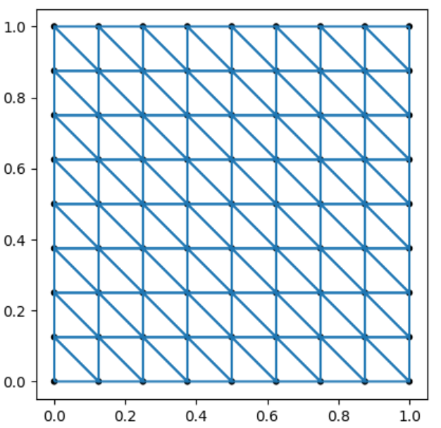
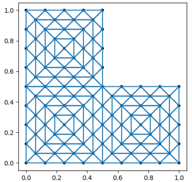
Figure 2: Left: unit square domain with uniform right triangular mesh ($h=\frac{1}{8}$). Right: L-shaped domain with uniform crossed triangular mesh $(h=\frac{1}{8})$.

Table 1: Dimension, $N$, and the number of nonzeros, nnz, in the system matrix for $u\in DG_{k}(\Omega,\tau_{h}),\ \vec{v}\in RT_{k+1}(\Omega,\tau_{h}),\ \vec{\alpha}\in RT_{k+1}(\Omega,\tau_{h})$ on uniform meshes of the unit square domain in 2D.

	$k=0$		$k=1$		$k=2$
$1/h$	$N$	nnz	$N$	nnz	$N$	nnz
$2^{6}$	33,024	352,768	107,008	2,762,752	221,952	10,179,072
$2^{7}$	131,584	1,410,048	427,008	11,046,912	886,272	40,707,072
$2^{8}$	525,312	5,638,144	1,705,984	44,179,456	3,542,016	162,809,856
$2^{9}$	2,099,200	22,548,480	6,819,840	176,701,440	14,161,920	651,202,560

We present two-dimensional numerical experiments in three parts. First, in Subsection 6.1.1, we investigate the convergence of our finite-element methods for sufficiently smooth exact solutions (as covered by our analysis), including the classical biharmonic problem with the clamped boundary conditions (requiring the use of the Nitsche penalty method). Then, in Subsection 6.1.2, we consider the case of exact solutions, $u_{ex}\notin H^{4}(\Omega)$, where convergence rates require further analysis. We demonstrate that, in certain cases, our method does not converge to the exact solution of the biharmonic equation if that solution does not lie in $H^{4}(\Omega)$ (i.e. in some cases it is not merely a matter of degraded convergence rates). Finally, in Subsection 6.1.3, we provide a comparison between direct solvers and the multigrid-preconditioned FGMRES algorithm for $H^{2}$ elliptic problems with $c_{0}\geq 0$ and $c_{1}>0$, as well as multigrid-preconditioned FGMRES iteration counts for the biharmonic problem with clamped boundary conditions, which is challenging due to the inclusion of the Nitsche boundary terms.

6.1.1 Smooth solutions

Here, we consider the unit square domain with two exact solutions, one that is smooth (in $C^{\infty}(\Omega)$), $u_{1ex}=\sin(2\pi x)\cos(3\pi y)$, and one that is in $H^{4}(\Omega)$, but not $H^{5}(\Omega)$, $u_{2ex}=\left(\sin(2\pi x)+x^{\frac{9}{2}}\right)\left(\cos(3\pi y)+y^{\frac{17}{4}}\right)$. In the results that follow, we plot $\log(R_{e}(\cdot,h))$ against $\log_{2}(1/h)$, so that the slopes of the lines represent the experimentally measured convergence rates for $(u,\vec{v},\vec{\alpha})\in DG_{k}(\Omega,\tau_{h})\times RT_{k+1}(\Omega,\tau_{h})\times RT_{k+1}(\Omega,\tau_{h})$, for $k\in\{0,1,2\}$. In the examples in this subsection, filled discs denote the measured $(u,\vec{v})$ error in the $L^{2}\times H(\text{div})$ norm, and squares denote the error in $\vec{\alpha}$ measured in the $H(\text{div})$ norm.

Let $\partial\Omega=\Gamma_{N}\cup\Gamma_{S}\cup\Gamma_{E}\cup\Gamma_{W}$, meaning the North, South, East, and West faces of the square. Figure 3 presents results for the problem with $c_{0}=0$ and $c_{1}=1$ with boundary $\partial\Omega=\Gamma_{0}\cup\Gamma_{3}$, where $\Gamma_{0}=\Gamma_{E}\cup\Gamma_{W}$, and $\Gamma_{3}=\Gamma_{N}\cup\Gamma_{S}$. Figure 4 presents results when $c_{0}=2$, $c_{1}=4$, and $\partial\Omega=\Gamma_{0}\cup\Gamma_{2}\cup\Gamma_{3}$ with $\Gamma_{0}=\Gamma_{E}\cup\Gamma_{W}$, $\Gamma_{2}=\Gamma_{S}$, and $\Gamma_{3}=\Gamma_{N}$. Since we omit $\Gamma_{1}$ from these examples, there is no need to use the Nitsche boundary terms considered in that case. We note that we see optimal convergence for all $k$ with $(u,\vec{v})$ in the $L^{2}\times H(\text{div})$ norm and $\vec{\alpha}$ in the $H(\text{div})$ norm for the smooth exact solution, $u_{1ex}$, on the left of these figures. Considering the $H^{4}(\Omega)$ solution, $u_{2ex}$, on the right, we see optimal convergence for small $k$, but degraded performance for $k=2$, where the lack of smoothness in $\alpha$ is reflected in the numerical results. These results are consistent with the analysis in Corollaries 13 and 14, although we note that the $H^{4}(\Omega)$ case outperforms the expected convergence from the analysis.

Figure 3: Relative approximation errors and rate of convergence for the unit square domain with $c_{0}=0,\ c_{1}=1,\ \partial\Omega=\Gamma_{0}\cup\Gamma_{3}$ and $(u,\vec{v},\vec{\alpha})\in DG_{k}(\Omega,\tau_{h})\times RT_{k+1}(\Omega,\tau_{h})\times RT_{k+1}(\Omega,\tau_{h})$, $k\in{0,1,2}$. Blue, red, and green lines present results for $k=0,1,2$, respectively. Filled discs denote the measured $(u,\vec{v})$ error in the $L^{2}\times H(\text{div})$ norm, and squares denote the error in $\vec{\alpha}$ measured in the $H(\text{div})$ norm. Reference lines of slopes -1, -2, and -3 approximate convergence rates. Left: smooth solution $u_{ex}=u_{1ex}$. Right: rough solution $u_{ex}=u_{2ex}$.

Figure 4: Relative approximation errors and rates of convergence for the unit square domain with $c_{0}=2,\ c_{1}=4,\ \partial\Omega=\Gamma_{0}\cup\Gamma_{2}\cup\Gamma_{3}$ and $(u,\vec{v},\vec{\alpha})\in DG_{k}(\Omega,\tau_{h})\times RT_{k+1}(\Omega,\tau_{h})\times RT_{k+1}(\Omega,\tau_{h})$, $k\in{0,1,2}$. Blue, red, and green lines present results for $k=0,1,2$, respectively. Filled discs denote the measured $(u,\vec{v})$ error in the $L^{2}\times H(\text{div})$ norm, and squares denote the error in $\vec{\alpha}$ measured in the $H(\text{div})$ norm. Reference lines of slopes -1, -2, and -3 approximate convergence rates. Left: smooth solution $u_{ex}=u_{1ex}$. Right: rough solution $u_{ex}=u_{2ex}$.

We next consider the classical biharmonic problem. Figure 5 shows results for the case where the exact solution is $u_{1ex}$ and $\partial\Omega=\Gamma_{0}\cup\Gamma_{1}\cup\Gamma_{2}$, and we take $(u,\vec{v},\vec{\alpha})\in DG_{2}(\Omega,\tau_{h})\times RT_{3}(\Omega,\tau_{h})\times RT_{3}(\Omega,\tau_{h})$. For this choice ($k=2$), Corollary 16 gives an expected convergence rate of $\mathcal{O}(h^{2})$ for $(u,\vec{v})$ and of $\mathcal{O}(h)$ for $\vec{\alpha}$. In contrast with that result, we observe almost $\mathcal{O}(h^{5/2})$ for $(u,\vec{v})$ in the modified $L^{2}\times H(\text{div})$ norm and $\mathcal{O}(h^{3/2})$ convergence for $\vec{\alpha}$.

Remark 4.

For the right-triangular meshes given in Figure 2 (Left), $\gamma_{1}(2)\approx 41$ and $\gamma_{1}(3)\approx 62$. Therefore, we choose $\lambda=125,\ \text{and}\ 210$ respectively for the numerical results given in Figure 5 and Table 6. Note that, for both cases, $\lambda>3\gamma_{1}$, which is necessary to satisfy the coercivity condition (4) for the bilinear form $\hat{a}$.

Figure 5: Relative approximation errors and rate of convergence for the biharmonic problem in the unit square domain and $\partial\Omega=\Gamma_{0}\cup\Gamma_{1}\cup\Gamma_{3}$. Filled discs denote the measured $(u,v)$ error in the $L^{2}\times H(\text{div})$ norm, and squares denote the error in $\alpha$ measured in the $H(\text{div})$ norm. Reference lines of slopes $-3/2$ and $-5/2$ approximate convergence rates. The exact solution is $C^{\infty}$, $u_{ex}=u_{1ex}$.

6.1.2 Nonsmooth solutions

In this section, we consider examples that do not conform to the theory presented above, with a variety of exact solutions that are less regular than $u\in H^{4}(\Omega)$. To gain insight into the structure of the errors in these cases, we present errors separately for each of $u$ (measured in the $L^{2}$ norm), $\vec{v}$, and $\vec{\alpha}$ (both measured in the $H(\text{div})$ norm), with triangles denoting measured errors in $u$, asterisks denoting measured errors in $\vec{v}$, and squares denoting the error in $\vec{\alpha}$.

In Figure 6, we consider the unit square domain with nonsmooth solution, $u_{3ex}=\left(\sin(2\pi x)+x^{\frac{7}{2}}\right)\left(\cos(3\pi y)+y^{\frac{13}{4}}\right)\in H^{3}(\Omega)$, noting that $u_{3ex}\notin H^{4}(\Omega)$. Figure 6 presents convergence results for $(u,\vec{v},\vec{\alpha})\in DG_{k}(\Omega,\tau_{h})\times RT_{k+1}(\Omega,\tau_{h})\times RT_{k+1}(\Omega,\tau_{h})$, for $k\in\{0,1,2\}$, with values of $c_{0}$ and $c_{1}$ and boundary conditions matching those considered in Figure 3 (at left) and Figure 4 (at right). Table 2 summarizes the measured convergence rates from this data, using the points at $\log_{2}(1/h)=8\text{ and }9$. While our analysis does not cover this case, we observe that our mixed formulation converges suboptimally to the correct solution. For the lowest-order discretization, we see convergence that is relatively good for all three components of the solution (but still somewhat suboptimal compared to the $\mathcal{O}(h)$ solution error we might hope to see), while we see diverging approximations of $\alpha$ for $k=1$ and $2$, with convergence rates of $\mathcal{O}(h^{1/4})$ for $u$ and $\vec{v}$. It is natural to speculate that this occurs since the solution is in $H^{13/4-\epsilon}(\Omega)$ for any $\epsilon>0$, but we leave analysis of this case for future work.

Figure 6: Relative approximation errors for the unit square domain with nonsmooth solution, $u_{3ex}\in H^{3}(\Omega)$. Triangles denote the measured error in $u$ in the $L^{2}$ norm, stars denote the measured error in $\vec{v}$ in the $H(\text{div})$ norm, and squares denote the measured error in $\vec{\alpha}$ in the $H(\text{div})$ norm. Blue, red, and green lines present results for $k=0,1,2$, respectively. Left: $c_{0}=0$, $c_{1}=1$, and $\partial\Omega=\Gamma_{0}\cup\Gamma_{3}$. Right: $c_{0}=2$, $c_{1}=4$, and $\partial\Omega=\Gamma_{0}\cup\Gamma_{2}\cup\Gamma_{3}$.

Table 2: Experimental convergence rates for the unit square domain with exact solution $u_{ex}=\left(\sin(2\pi x)+x^{7/2}\right)\left(\cos(3\pi y)+y^{13/4}\right)$, and $(u,\vec{v},\vec{\alpha})\in DG_{k}\times RT_{k+1}\times RT_{k+1}$, $k\in\{0,1,2\}$. Errors in $u$ are measured in the $L^{2}$ norm and errors in $\vec{v}$ and $\vec{\alpha}$ are measured in the $H(\text{div})$ norm. Dashes mean that we do not observe convergence.

	Figure 6 (left)	Figure 6 (right).
$k=0$	(0.93, 1.00, 0.70)	(0.42, 0.98, 0.70)
$k=1$	(0.25, 0.27, -)	(0.26, 0.24, -)
$k=2$	(0.25, 0.25, -)	(0.25, 0.25, -)

In the next experiments, we consider the L-shaped domain with $\partial\Omega=\Gamma_{0}$ and discretizations with $k\in\{0,1,2\}$. Here, we consider harmonic functions as exact solutions, given in polar coordinates as $u_{p}=r^{2p/3}\sin(2p\theta/3)$, for $p\in\{1,2,4\}$, and impose nonhomogeneous boundary conditions to match the solution along the boundary (enforced weakly, by including the boundary integrals generated when integrating by parts on Equations (32) and (33) to get Equations (35) and (36), respectively, with known values for $\nabla\cdot\vec{v}_{p}=\Delta u_{p}$ and $u_{p}$). We place the origin for the $(r,\theta)$ coordinates at the re-entrant corner at $(1/2,1/2)$, and measure the angle counterclockwise from the positive $y$-direction from this origin (see Figure 2 (right)). This results in homogeneous Dirichlet BCs for $u$ along the two edges incident to the re-entrant corner, but non-homogeneous values on the other four edges of the domain. Note that $(u_{p},\vec{v}_{p})$ are in $H^{1+2p/3-\epsilon}(\Omega)\times[H^{2p/3-\epsilon}(\Omega)]^{2}$ [66, Theorem 1.2.18], for any $\epsilon>0$, but not in $H^{1+2p/3}(\Omega)\times[H^{2p/3}(\Omega)]^{2}$, with $\vec{\alpha}_{p}=\vec{0}$. Thus, we might expect to correctly compute $\vec{\alpha}_{p}$, since it is trivially represented in the $RT_{k+1}$ space for all $k\geq 0$, but expect, at best, to obtain $\mathcal{O}(h^{\min\{1+2p/3,k+1\}})$ and $\mathcal{O}(h^{\min\{2p/3,k+1\}})$ convergence rates for $u_{p}$ in the $L^{2}$ norm and $\vec{v}_{p}$ in the $H(\text{div})$ norm, respectively. Considering that the error analysis above is done in the $L^{2}\times H(\text{div})$ product norm, it may even be reasonable to expect no better than $\mathcal{O}(h^{\min\{2p/3,k+1\}})$ convergence rates for both $u_{p}$ and $\vec{v}_{p}$.

From most to least smooth, we show results for this problem for $p=4$ in Figure 7 and for $p=2$ (at right) and $p=1$ (at left) in Figure 8. In all cases, we omit reporting results for $\vec{\alpha}_{p}=\vec{0}$, as the absolute error is always at the level of machine precision. Table 3 summarizes convergence rates, measuring the slopes of this data using the points at $\log_{2}(1/h)=8\text{ and }9$. For $p=2$ and $p=4$, we observe best possible convergence rates for both $u$ and $\vec{v}$, while we observe the best possible convergence rate for $\vec{v}$, but slightly less than this for $u$, when $p=1$. (Preliminary numerical experiments, not reported here, showed that multiplying a harmonic function by a smooth function, to yield nonzero $\vec{\alpha}$ resulted in similarly reduced convergence orders for $\vec{\alpha}$, including a lack of convergence when taking $k=0$). Clearly for $p=1$, $u_{p}\notin H^{2}(\Omega)$, so our proposed method is converging to a function that cannot be a true solution of the biharmonic problem, but is admitted by the weaker mixed formulation that requires only $u\in L^{2}(\Omega)$ and $\vec{v}=\nabla u\in H(\text{div};\Omega)$. This is confirmed by computing the smallest eigenvalue of this discretization of the biharmonic, which yields a value of approximately 1,486 on a mesh with $h=1/128$ discretized with $u\in DG_{1}(\Omega,\tau_{h})$ and $\vec{v},\vec{\alpha}\in RT_{2}(\Omega,\tau_{h})$, close to the square of the smallest Laplacian eigenvalue and not the true smallest biharmonic eigenvalue of approximately 2,641 (cf., [67]). This is reminiscent of the Sapondjan paradox, where solving the biharmonic problem via a mixed formulation involving two Poisson problems gives the wrong solution on nonconvex domains [68, pg. 268]. Whether anything can be proven about the convergence to solutions with degraded regularity (meaning $u\in H^{2}(\Omega)$, but not $H^{4}(\Omega)$) remains an open question for future research that is clearly complicated by the weaker spaces used in the mixed formulation.

Figure 7: Relative approximation errors for the biharmonic problem on the L-shaped domain with $\partial\Omega=\Gamma_{0}$ with triangles denoting the measured $u$ error in the $L^{2}$ norm, and stars denoting the error in $\vec{v}$ measured in the $H(\text{div})$ norm with $u_{ex}=u_{4}$. Blue, red, and green lines present results for $k=0,1,2$, respectively.

Figure 8: Relative approximation errors for the biharominc problem on the L-shaped domain with $\partial\Omega=\Gamma_{0}$ with triangles denoting the measured $u$ error in the $L^{2}$ norm, and stars denoting the error in $\vec{v}$ measured in the $H(\text{div})$ norm. Blue, red, and green lines present results for $k=0,1,2$, respectively. Left: $u_{ex}=u_{1}$. Right: $u_{ex}=u_{2}$.

Table 3: Experimental convergence rates for the L-shaped domain with $\partial\Omega=\Gamma_{0}$ and $(u,\vec{v},\vec{\alpha})\in DG_{k}\times RT_{k+1}\times RT_{k+1}$, $k\in\{0,1,2\}$. The exact solutions are $u_{p}=r^{2p/3}\sin(2p\theta/3)$, $p=1,2,4$. Errors in $u$ are measured in the $L^{2}$ norm and errors in $\vec{v}$ are measured in the $H(\text{div})$ norm. Results for $\vec{\alpha}_{p}=\vec{0}$ are omitted as it is exactly approximated by this discretization.

	Figure 8 (left, $p=1$)	Figure 8 (right, $p=2$)	Figure 7 ($p=4$)
$k=0$	(1.00, 0.66)	(1.00, 1.00)	(1.00, 1.00)
$k=1$	(1.36, 0.67)	(2.00, 1.33)	(2.00, 2.00)
$k=2$	(1.34, 0.67)	(2.33, 1.33)	(3.00, 2.66)

6.1.3 Monolithic multigrid solvers

Finally, we report on the effectiveness of the monolithic multigrid preconditioner proposed in Section 5, using the exact solution, $u_{1ex}$. To demonstrate the effectiveness of the monolithic multigrid preconditioner, Table 4 presents iteration counts and CPU times to solution for both the multigrid-preconditioned FGMRES iterations and the use of a direct solver (MUMPS [69], via the PETSc interface) for the unit square domain, with $(u,\vec{v},\vec{\alpha})\in DG_{2}(\Omega,\tau_{h})\times RT_{3}(\Omega,\tau_{h})\times RT_{3}(\Omega,\tau_{h})$ and $\partial\Omega=\Gamma_{0}\cup\Gamma_{3}$. We note that the iteration counts for monolithic multigrid-preconditioned FGMRES are consistent through all runs and mesh sizes, and that the scaling of wall-clock time for this approach is $\mathcal{O}({\color[rgb]{0,0,0}N})$ or better throughout. While the direct solver is faster for small mesh sizes, we see worse than $\mathcal{O}({\color[rgb]{0,0,0}N})$ scaling for the wall-clock time with MUMPS at larger mesh sizes, showing the expected behaviour. Moreover, as we vary the number of processors over which we parallelize the computation, we see that, for sufficiently large problems, we have reasonable strong parallel scalability with the monolithic multigrid solver, although MUMPS is always faster than our multigrid implementation for this two-dimensional problem. Table 5 presents the case of $\partial\Omega=\Gamma_{0}\cup\Gamma_{2}\cup\Gamma_{3}$, $(u,\vec{v},\vec{\alpha})\in DG_{1}(\Omega,\tau_{h})\times RT_{2}(\Omega,\tau_{h})\times RT_{2}(\Omega,\tau_{h})$. As we increase the number of processors from 4 to 16, we see better performance with the multigrid solver than the direct solver. Again, we have good strong parallel scalability with the monolithic multigrid solver, showing 3.83x speedup for the $1024^{2}$ mesh, while the direct solver (MUMPS) shows only 1.55x speedup.

Table 4: Wall-clock time (in seconds) and iterations to convergence with varying numbers of processors, $p$, for monolithic multigrid and a direct solver (MUMPS) for the unit square domain with $c_{0}=0$, $c_{1}=1$, $\partial\Omega=\Gamma_{0}\cup\Gamma_{3}$ and $(u,\vec{v},\vec{\alpha})\in DG_{2}(\Omega,\tau_{h})\times RT_{3}(\Omega,\tau_{h})\times RT_{3}(\Omega,\tau_{h})$.

${h^{-1}}$	Monolithic			MUMPS
	Iterations	Time ($p=1$)	Time ($p=4$)	Time ($p=1$)	Time ($p=4$)
$2^{6}$	5	31.48	15.45	6.07	4.11
$2^{7}$	5	97.30	37.04	16.55	9.35
$2^{8}$	5	386.82	137.35	74.39	39.19
$2^{9}$	5	1553.12	623.34	358.06	183.83

Table 5: Wall-clock time (in seconds) and iterations to convergence with varying numbers of processors, $p$, for monolithic multigrid and a direct solver (MUMPS) for the unit square domain with $c_{0}=2$, $c_{1}=4$, $\partial\Omega=\Gamma_{0}\cup\Gamma_{2}\cup\Gamma_{3}$ and $(u,\vec{v},\vec{\alpha})\in DG_{1}(\Omega,\tau_{h})\times RT_{2}(\Omega,\tau_{h})\times RT_{2}(\Omega,\tau_{h})$.

$h^{-1}$	Monolithic			MUMPS
	Iterations	Time ($p=4$)	Time ($p=16$)	Time ($p=4$)	Time ($p=16$)
$2^{7}$	5	19.00	10.18	6.22	4.46
$2^{8}$	5	48.62	18.53	17.96	12.24
$2^{9}$	5	178.60	58.65	83.58	53.89
$2^{10}$	5	854.42	223.28	387.61	250.35

Finally, we consider the classical biharmonic operator with clamped boundary conditions, i.e., $c_{0}=c_{1}=0$ and $\partial\Omega=\Gamma_{1}$ and $(u,\vec{v},\vec{\alpha})\in DG_{3}(\Omega,\tau_{h})\times RT_{4}(\Omega,\tau_{h})\times RT_{4}(\Omega,\tau_{h})$. Table 6 shows the effectiveness of the monolithic multigrid solver with an $\mathcal{O}(h^{-1})$ weight on the auxiliary operator. Dashes in the table mean that more than 100 iterations were required to converge when the residual norm or its relative reduction is less than ${\color[rgb]{0,0,0}10^{-12}}$. We note that, due to a technical limitation in PCPATCH (where Nitsche boundary terms cannot be treated), these results use an alternate implementation of the star relaxation scheme that is less efficient than PCPATCH. Consequently, we do not report timings for these experiments, as they are not comparable to the timings reported elsewhere in this paper.

Table 6: Number of iterations to converge with different weights on the auxiliary operator. Here $(u,\vec{v},\vec{\alpha})\in DG_{3}(\Omega,\tau_{h})\times RT_{4}(\Omega,\tau_{h})\times RT_{4}(\Omega,\tau_{h})$. A dash means that convergence was not achieved in 100 iterations.

	1	10	20	40	80	$h^{-1}$
$2^{6}$	29	11	11	10	10	10
$2^{7}$	-	17	13	10	10	10
$2^{8}$	-	46	22	16	12	10
$2^{9}$	-	-	-	-	-	9

6.2 $3D$ experiments

Here, we consider a test case on the unit cube, with right-hand side and boundary conditions chosen so that the exact solution is $u_{ex}=\sin(2\pi x)\cos(3\pi y)\sinh(\pi z)$. Finite-element convergence is demonstrated in Figure 9 for $k\in\{0,1,2\}$ with $\partial\Omega=\Gamma_{0}\cup\Gamma_{2}\cup\Gamma_{3}$, with $\Gamma_{0}$ corresponding to $z=0$ and $z=1$, $\Gamma_{2}$ corresponding to $y=0$ and $y=1$, and $\Gamma_{3}$ corresponding to $x=0$ and $x=1$, showing convergence consistent with the analysis of Corollary 14. Table 7 details the performance of the monolithic multigrid-preconditioned FGMRES solver for $k=0$, compared with a standard direct solver (MUMPS). We see excellent performance of the monolithic multigrid method, with iteration counts that are independent of problem size and CPU time scaling linearly with problem size, and decreasing with parallelization for sufficiently large problems. In contrast, we see the expected rapid growth of required CPU times for MUMPS, and suboptimal parallel scaling, showing the utility and power of the monolithic multigrid approach.

Figure 9: Relative approximation errors and rates of convergence for the unit cube domain $\partial\Omega=\Gamma_{0}\cup\Gamma_{2}\cup\Gamma_{3}$, $c_{0}=4$ and $c_{1}=2$. Blue, red, and green lines present results for $k=0,1,2$, respectively. Reference lines of slopes -1, -2, and -3 approximate convergence rates.

Table 7: Wall-clock time (in seconds) and iterations to convergence with varying numbers of processors, $p$, for monolithic multigrid and a direct solver (MUMPS) for the unit cube domain with $c_{0}=4$, $c_{1}=2$, $\partial\Omega=\Gamma_{0}\cup\Gamma_{2}\cup\Gamma_{3}$ and $(u,\vec{v},\vec{\alpha})\in DG_{0}(\Omega,\tau_{h})\times RT_{1}(\Omega,\tau_{h})\times RT_{1}(\Omega,\tau_{h})$.

$h^{-1}$	Monolithic			MUMPS
	Iterations	Time ($p=1$)	Time ($p=8$)	Time ($p=1$)	Time ($p=8$)
$2^{3}$	9	8.05	5.80	2.08	1.92
$2^{4}$	9	20.07	7.34	6.80	2.99
$2^{5}$	9	229.04	37.59	124.05	39.22
$2^{6}$	9	1847.76	276.34	4903.83	1148.47

7 Conclusion

We consider the mixed finite-element approximation of solutions to $H^{2}$-elliptic fourth-order problems, achieved by the transformation of the fourth-order equation into a system of PDEs. We find that under natural assumptions on the coefficients of the problem, three combinations of boundary conditions lead to optimal finite-element convergence. For the fourth case of boundary conditions (“clamped” boundary conditions, on the solution and its normal derivative), suboptimal rates of convergence are expected and observed when implemented using Nitsche’s method. While the approach is applicable in both two and three dimensions, we note that it is particularly attractive in 3D, where the cost of conforming methods is prohibitive. It remains an open question whether or not it is possible to employ alternative approaches (such as adapting the Nitsche boundary conditions, or the use of alternative penalty approaches) to regain optimal finite-element convergence for the boundary conditions where suboptimal convergence is proven and observed here. As is common for mixed formulations, the approach we propose herein has higher regularity requirements to guarantee convergence than other possible approaches. Numerical results suggest that acceptable convergence can be achieved in some cases when this regularity is not present (for a solution in $H^{3}(\Omega)$ but not $H^{4}(\Omega)$), but in some cases inadmissible solutions are found (with $u\notin H^{2}(\Omega)$) due to the weaker spaces used. Understanding convergence in these cases is a target for future research. We additionally propose a monolithic multigrid algorithm with optimal scaling for the resulting discrete linear systems. For three-dimensional problems, this approach yields a preconditioned FGMRES iteration that dramatically outperforms state-of-the-art direct solvers.

References

- [1] G. Engel, K. Garikipati, T. J. R. Hughes, M. G. Larson, L. Mazzei, R. L. Taylor, Continuous/discontinuous finite element approximations of fourth-order elliptic problems in structural and continuum mechanics with applications to thin beams and plates, and strain gradient elasticity, Comput. Methods Appl. Mech. Engrg. 191 (34) (2002) 3669–3750. doi:10.1016/S0045-7825(02)00286-4.
- [2] M. Y. Pevnyi, J. V. Selinger, T. J. Sluckin, Modeling smectic layers in confined geometries: Order parameter and defects, Phys. Rev. E 90 (3) (2014) 032507.
- [3] P. Monk, A mixed finite element method for the biharmonic equation, SIAM J. Numer. Anal. 24 (4) (1987) 737–749. doi:10.1137/0724048.
- [4] P. G. Ciarlet, The finite element method for elliptic problems, North-Holland Publishing Co., Amsterdam-New York-Oxford, 1978, studies in Mathematics and its Applications, Vol. 4.
- [5] R. C. Kirby, A. Logg, M. E. Rognes, A. R. Terrel, Common and unusual finite elements, in: Automated Solution of Differential Equations by the Finite Element Method, Springer, 2012, pp. 95–119.
- [6] R. Kirby, L. Mitchell, Code generation for generally mapped finite elements, ACM Trans. Math. Software 45 (2019) 1–23. doi:10.1145/3361745.
- [7] S. C. Brenner, L. R. Scott, The mathematical theory of finite element methods, 3rd Edition, Vol. 15 of Texts in Applied Mathematics, Springer, New York, 2008. doi:10.1007/978-0-387-75934-0.
- [8] M. Wang, J. Xu, The Morley element for fourth order elliptic equations in any dimensions, Numer. Math. 103 (1) (2006) 155–169. doi:10.1007/s00211-005-0662-x.
- [9] P. Wang, L. Jiang, S. Chen, A nonconforming scheme for non-Fickian flow in porous media, J. Inequal. Appl. (2017) Paper No. 142, 16doi:10.1186/s13660-017-1419-7.
- [10] S. C. Brenner, L.-Y. Sung, interior penalty methods for fourth order elliptic boundary value problems on polygonal domains, J. Sci. Comput. 22/23 (2005) 83–118. doi:10.1007/s10915-004-4135-7.
- [11] S. C. Brenner, S. Gu, T. Gudi, L.-Y. Sung, A quadratic interior penalty method for linear fourth order boundary value problems with boundary conditions of the Cahn-Hilliard type, SIAM J. Numer. Anal. 50 (4) (2012) 2088–2110. doi:10.1137/110847469.
- [12] I. Babuška, M. Zlámal, Nonconforming elements in the finite element method with penalty, SIAM J. Numer. Anal. 10 (1973) 863–875. doi:10.1137/0710071.
- [13] T. D. Nguyen, Discontinuous Galerkin formulations for thin bending problems, Ph.D. thesis, Delft University of Technology (2008).
- [14] G. A. Baker, Finite element methods for elliptic equations using nonconforming elements, Math. Comp. 31 (137) (1977) 45–59. doi:10.2307/2005779.
- [15] E. Süli, I. Mozolevski, -version interior penalty DGFEMs for the biharmonic equation, Comput. Methods Appl. Mech. Engrg. 196 (13-16) (2007) 1851–1863. doi:10.1016/j.cma.2006.06.014.
- [16] L. Banz, B. P. Lamichhane, E. P. Stephan, A new three-field formulation of the biharmonic problem and its finite element discretization, Numer. Methods Partial Differential Equations 33 (1) (2017) 199–217. doi:10.1002/num.22082.
- [17] X.-L. Cheng, W. Han, H.-C. Huang, Some mixed finite element methods for biharmonic equation, J. Comput. Appl. Math. 126 (1-2) (2000) 91–109. doi:10.1016/S0377-0427(99)00342-8.
- [18] Z. Li, S. Zhang, A stable mixed element method for the biharmonic equation with first-order function spaces, Comput. Methods Appl. Math. 17 (4) (2017) 601–616. doi:10.1515/cmam-2017-0002.
- [19] E. M. Behrens, J. Guzmán, A mixed method for the biharmonic problem based on a system of first-order equations, SIAM J. Numer. Anal. 49 (2) (2011) 789–817. doi:10.1137/090775245.
- [20] D. S. Malkus, T. J. Hughes, Mixed finite element methods, reduced and selective integration techniques: a unification of concepts, Comput. Meth. Appl. Mech. Eng 15 (1) (1978) 63–81.
- [21] L. Banz, J. Petsche, A. Schröder, Two stabilized three-field formulations for the biharmonic problem, in: Chemnitz Finite Element Symposium, Springer, 2017, pp. 41–55.
- [22] D. Gallistl, Stable splitting of polyharmonic operators by generalized Stokes systems, Math. Comp. 86 (308) (2017) 2555–2577. doi:10.1090/mcom/3208.
- [23] I. Babuška, J. Osborn, J. Pitkäranta, Analysis of mixed methods using mesh dependent norms, Math. Comp. 35 (152) (1980) 1039–1062. doi:10.2307/2006374.
- [24] W. Krendl, K. Rafetseder, W. Zulehner, A decomposition result for biharmonic problems and the Hellan-Herrmann-Johnson method, Electron. Trans. Numer. Anal. 45 (2016) 257–282.
- [25] D. Pauly, W. Zulehner, The divDiv-complex and applications to biharmonic equations, Appl. Anal. 99 (9) (2020) 1579–1630. doi:10.1080/00036811.2018.1542685.
- [26] C. Johnson, J. Pitkäranta, Analysis of some mixed finite element methods related to reduced integration, Math. Comp. 38 (158) (1982) 375–400. doi:10.2307/2007276.
- [27] M. Ilyas, B. Lamichhane, A three-field formulation of the Poisson problem with Nitsche approach, ANZIAM Journal 59 (11 2017). doi:10.21914/anziamj.v59i0.12645.
- [28] M. Juntunen, R. Stenberg, Nitsche’s method for general boundary conditions, Math. Comp. 78 (267) (2009) 1353–1374. doi:10.1090/S0025-5718-08-02183-2.
- [29] I. Babuška, The finite element method with penalty, Math. Comp. 27 (1973) 221–228. doi:10.2307/2005611.
- [30] J.-P. Aubin, Approximation of elliptic boundary-value problems, Wiley-Interscience [A division of John Wiley & Sons, Inc.], New York-London-Sydney, 1972, pure and Applied Mathematics, Vol. XXVI.
- [31] J. Nitsche, Über ein Variationsprinzip zur Lösung von Dirichlet-Problemen bei Verwendung von Teilräumen, die keinen Randbedingungen unterworfen sind, Abhandlungen aus dem Mathematischen Seminar der Universität Hamburg 36 (1) (1971) 9–15. doi:10.1007/bf02995904.
- [32] J. Freund, R. Stenberg, On weakly imposed boundary conditions for second order problems, Proceedings of the Ninth International Conference on Finite Elements in Fluids (1995) 327–336.
- [33] A. Embar, J. Dolbow, I. Harari, Imposing Dirichlet boundary conditions with Nitsche’s method and spline-based finite elements, Int. J. Numer. Methods Engrg. 83 (7) (2010) 877–898. doi:10.1002/nme.2863.
- [34] J. Benzaken, J. A. Evans, S. F. McCormick, R. Tamstorf, Nitsche’s method for linear Kirchhoff–Love shells: Formulation, error analysis, and verification, Comput. Methods Appl. Mech. Engrg. 374 (2021) 113544. doi:https://doi.org/10.1016/j.cma.2020.113544.
- [35] M. Benzi, G. H. Golub, J. Liesen, Numerical solution of saddle point problems, Acta Numer. 14 (2005) 1–137. doi:10.1017/S0962492904000212.
- [36] H. C. Elman, D. J. Silvester, A. J. Wathen, Finite elements and fast iterative solvers: with applications in incompressible fluid dynamics, Numerical Mathematics and Scientific Computation, Oxford University Press, New York, 2005.
- [37] P. E. Farrell, L. Mitchell, F. Wechsung, An augmented Lagrangian preconditioner for the 3D stationary incompressible Navier–Stokes equations at high Reynolds number, SIAM J. Sci. Comput. 41 (5) (2019) A3073–A3096. doi:10.1137/18M1219370.
- [38] M. F. Murphy, G. H. Golub, A. J. Wathen, A note on preconditioning for indefinite linear systems, SIAM J. Sci. Comput. 21 (6) (2000) 1969–1972. doi:10.1137/S1064827599355153.
- [39] J. H. Adler, T. R. Benson, S. P. MacLachlan, Preconditioning a mass-conserving discontinuous Galerkin discretization of the Stokes equations, Numer. Linear Algebra Appl. 24 (3) (2017) e2047, 23. doi:10.1002/nla.2047.
- [40] J. H. Adler, T. J. Atherton, T. R. Benson, D. B. Emerson, S. P. MacLachlan, Energy minimization for liquid crystal equilibrium with electric and flexoelectric effects, SIAM J. Sci. Comput. 37 (5) (2015) S157–S176. doi:10.1137/140975036.
- [41] J. H. Adler, T. Benson, E. C. Cyr, P. E. Farrell, S. MacLachlan, R. Tuminaro, Monolithic multigrid for magnetohydrodynamics, SIAM J. Sci. Comput. (2021) S70–S91doi:10.1137/20M1348364.
- [42] S. P. Vanka, Block-implicit multigrid solution of Navier-Stokes equations in primitive variables, J. Comput. Phys. 65 (1) (1986) 138–158. doi:10.1016/0021-9991(86)90008-2.
- [43] P. E. Farrell, M. G. Knepley, F. Wechsung, L. Mitchell, PCPATCH: software for the topological construction of multigrid relaxation methods, ACM Transactions on Mathematical SoftwareIn press (2021). arXiv:1912.08516.
- [44] S. C. Brenner, L.-Y. Sung, Multigrid algorithms for interior penalty methods, SIAM J. Numer. Anal. 44 (1) (2006) 199–223. doi:10.1137/040611835.
- [45] S. C. Brenner, S. Gu, L.-Y. Sung, Multigrid methods for the biharmonic problem with Cahn-Hilliard boundary conditions, in: R. Bank, M. Holst, O. Widlund, J. Xu (Eds.), Domain Decomposition Methods in Science and Engineering XX, Springer Berlin Heidelberg, Berlin, Heidelberg, 2013, pp. 127–134.
- [46] L. Chen, J. Hu, X. Huang, Multigrid methods for Hellan-Herrmann-Johnson mixed method of Kirchhoff plate bending problems, J. Sci. Comput. 76 (2) (2018) 673–696. doi:10.1007/s10915-017-0636-z.
- [47] D. Boffi, F. Brezzi, M. Fortin, Mixed finite element methods and applications, Vol. 44 of Springer Series in Computational Mathematics, Springer, Heidelberg, 2013. doi:10.1007/978-3-642-36519-5.
- [48] D. Braess, Finite elements, 3rd Edition, Cambridge University Press, Cambridge, 2007, theory, fast solvers, and applications in elasticity theory, Translated from the German by Larry L. Schumaker. doi:10.1017/CBO9780511618635.
- [49] D. N. Arnold, R. S. Falk, R. Winther, Preconditioning in and applications, Math. Comp. 66 (219) (1997) 957–984. doi:10.1090/S0025-5718-97-00826-0.
- [50] D. Arnold, R. Falk, R. Winther, Multigrid in and , Numer. Math. 85 (2) (2000) 197–217.
- [51] T. Warburton, J. S. Hesthaven, On the constants in -finite element trace inverse inequalities, Comput. Methods Appl. Mech. Engrg. 192 (25) (2003) 2765–2773. doi:10.1016/S0045-7825(03)00294-9.
- [52] B. Rivière, Discontinuous Galerkin methods for solving elliptic and parabolic equations: Theory and implementation, Vol. 35 of Frontiers in Applied Mathematics, Society for Industrial and Applied Mathematics (SIAM), Philadelphia, PA, 2008. doi:10.1137/1.9780898717440.
- [53] A. Ern, J.-L. Guermond, Finite elements I—Approximation and interpolation, Vol. 72 of Texts in Applied Mathematics, Springer, Cham, [2021] ©2021. doi:10.1007/978-3-030-56341-7.
- [54] V. Girault, P.-A. Raviart, Finite element methods for Navier-Stokes equations: Theory and algorithms, Vol. 5 of Springer Series in Computational Mathematics, Springer-Verlag, Berlin, 1986. doi:10.1007/978-3-642-61623-5.
- [55] A. Natale, J. Shipton, C. J. Cotter, Compatible finite element spaces for geophysical fluid dynamics, Dynamics and Statistics of the Climate System 1 (1) (11 2016). doi:10.1093/climsys/dzw005.
- [56] F. Brezzi, M. Fortin, Mixed and hybrid finite element methods, Vol. 15 of Springer Series in Computational Mathematics, Springer-Verlag, New York, 1991. doi:10.1007/978-1-4612-3172-1.
- [57] D. N. Arnold, R. S. Falk, J. Gopalakrishnan, Mixed finite element approximation of the vector Laplacian with Dirichlet boundary conditions, Math. Models Methods Appl. Sci. 22 (9) (2012) 1250024, 26. doi:10.1142/S0218202512500248.
- [58] Y. Saad, A flexible inner-outer preconditioned GMRES algorithm, SIAM J. Sci. Comput. 14 (2) (1993) 461–469. doi:10.1137/0914028.
- [59] S. P. MacLachlan, C. W. Oosterlee, Local Fourier analysis for multigrid with overlapping smoothers applied to systems of PDEs, Numer. Linear Algebra Appl. 18 (4) (2011) 751–774. doi:10.1002/nla.762.
- [60] F. Rathgeber, D. A. Ham, L. Mitchell, M. Lange, F. Luporini, A. T. McRae, G.-T. Bercea, G. R. Markall, P. H. Kelly, Firedrake: automating the finite element method by composing abstractions, ACM Trans. Math. Software 43 (3) (2017) 24.
- [61] R. C. Kirby, L. Mitchell, Solver composition across the PDE/linear algebra barrier, SIAM J. Sci. Comput. 40 (1) (2018) C76–C98.
- [62] K.-A. Mardal, R. Winther, Preconditioning discretizations of systems of partial differential equations, Numer. Lin. Alg. Appl. 18 (1) (2011) 1–40. doi:10.1002/nla.716.
- [63] R. C. Kirby, From functional analysis to iterative methods, SIAM Rev. 52 (2) (2010) 269–293. doi:10.1137/070706914.
- [64] S. Balay, S. Abhyankar, M. Adams, J. Brown, P. Brune, K. Buschelman, L. Dalcin, A. Dener, V. Eijkhout, W. Gropp, et al., PETSc users manual: Revision 3.10, Tech. rep., Argonne National Lab.(ANL), Argonne, IL (United States) (2018).
- [65] Software used in ‘A new mixed finite-element method for elliptic problems’ (oct 2022). doi:10.5281/zenodo.7184887.
- [66] P. Grisvard, Singularities in boundary value problems, Vol. 22, Springer, 1992.
- [67] S. C. Brenner, P. Monk, J. Sun, interior penalty Galerkin method for biharmonic eigenvalue problems, in: Spectral and high order methods for partial differential equations—ICOSAHOM 2014, Vol. 106 of Lect. Notes Comput. Sci. Eng., Springer, Cham, 2015, pp. 3–15. doi:10.1007/978-3-319-19800-2.
- [68] S. A. Nazarov, B. A. Plamenevsky, Elliptic problems in domains with piecewise smooth boundaries, Vol. 13 of De Gruyter Expositions in Mathematics, Walter de Gruyter & Co., Berlin, 1994. doi:10.1515/9783110848915.525.
- [69] P. R. Amestoy, I. S. Duff, J. Koster, J.-Y. L’Excellent, A fully asynchronous multifrontal solver using distributed dynamic scheduling, SIAM J. Matrix Anal. Appl. 23 (1) (2001) 15–41.