ElATools: A tool for analyzing anisotropic elastic properties of the 2D and 3D materials

Abstract

We introduce a computational method and a user-friendly code with a terminal-based graphical user interface (GUI), named ElATools, developed to analyze mechanical and anisotropic elastic properties. ElATools enables facile analysis of the second-order elastic stiffness tensor of two-dimensional (2D) and three-dimensional (3D) crystal systems. It computes and displays the main mechanical properties including the bulk modulus, Young’s modulus, shear modulus, hardness, p-wave modulus, universal anisotropy index, Chung-Buessem anisotropy index, log-Euclidean anisotropy parameter, Cauchy pressures, Poisson’s ratio, and Pugh’s ratio, using three averaging schemes of Voigt, Reuss, and Hill. It includes an online and offline database from the Materials Project with more than 13,000 elastic stiffness constants for 3D materials. The program supports output files of the well-known computational codes IRelast, IRelast2D, ElaStic, and AELAS. Four types of plotting and visualization tools are integrated to conveniently interface with GNUPLOT, XMGRACE, view3dscene and plotly libraries, offering immediate post-processing of the results. ElATools provides reliable means to investigate the mechanical stability based on the calculation of six (three) eigenvalues of the elastic tensor in 3D (2D) materials. It can efficiently identify anomalous mechanical properties, such as negative linear compressibility, negative Poisson’s ratio, and highly-anisotropic elastic modulus in 2D and 3D materials, which are central properties to design and develop high-performance nanoscale electromechanical devices. Moreover, ElATools can predict the behavior of the sound velocities and their anisotropic properties, such as acoustic phase/group velocities and power flow angles in materials, by solving the Christoffel equation. Six case studies on selected material systems, namely, ZnAu₂(CN)₄, CrB₂, $\delta$-phosphorene, Pd₂O₆Se₂ monolayer, and GaAs, and a hypothetical set of systems with cubic symmetry are presented to demonstrate the descriptive and predictive capabilities of ElATools.

Program summary
Title: ElATools
Licensing provisions: GNU General Public Licence 3.0
Nature of the problem: Identifying anisotropic elastic properties of 2D and 3D materials, and calculating acoustic phase and group velocities in homogeneous solids.
Solution method: Second-order elastic stiffness tensor analysis using transformation law and calculations of the elastic surfaces properties. Solving the Christoffel equation eigenvalue problem using diagonalization and calculations of the sound velocities.
Programming language: Fortran 90
Operating system: Unix/Linux/MacOS/Windows by Cygwin: http://www.cygwin.com/
Distribution format: tar.gz
Required routines/libraries: LaPack, Blas, and Plotly Javascript libraries, GNUPLOT, XMGRACE, view3dscene.
Computer: Any system with a Fortran 90 (F90) compiler
Memory: Up to 1 GB for any symmetry
Run time: Up to 70 seconds for any symmetry, and (400$\times$400) = ($\theta$$\times$$\phi$)-mesh in spherical coordinate
Documentation: Available at https://yalameha.gitlab.io/elastictools/index.html

I INTRODUCTION

The second-order elastic constants are essential materials parameters, playing pivotal roles in many research areas of engineering Ledbetter and Reed (1973); Li and Bradt (1987), medical Turner et al. (1990); Yoon and Newnham (1969), condensed matter physics  Saeidi et al. (2019a); Yalameha and Vaez (2018); Yalameha et al. (2020), materials science Tehrani and Brgoch (2019), geophysics Lay and Wallace (1995), and chemical Tatsumi et al. (2003). Moreover, the second-order elastic constants will contain information about how acoustic waves behave McSkimin (1950). Despite these critical practical features, the second-order elastic constants have been measured for a tiny fraction of known crystalline materials. The small data availability is due to the unavailability of large single crystals for many materials and the difficulty of precise experimental measurements Vacher and Boyer (1972). The lack of such experimental data limits the scientists’ ability to design and develop novel materials. With the development of high-performance computing resources and density functional theory (DFT) Parr and Yang (1995), the determination of elastic constants of many materials can become a reality. DFT is a robust technique able to solve many-body problems using Kohn-Sham equations Hohenberg and Kohn (1964); Kohn and Sham (1965), based on which several quantum-chemistry and solid-state physics software have been developed. A number of packages have been introduced to calculate the second-order elastic stiffness tensor of 2D and 3D crystals. For example, VASP Sun et al. (2003) can calculate second-order elastic constants using strain–stress relationships, and CRYSTAL14 Dovesi et al. (2014) can compute the piezoelectric and the photoelastic tensors. There is also some software capable of calculating the elastic constants using internal or external packages. For example, WIEN2k Blaha et al. (2020) uses internal packages such as IRelast Jamal et al. (2018) and Elast (for cubic systems) to calculate the second-order elastic constants, while ElaStic code is an external package Golesorkhtabar et al. (2013) used in Quantum Espresso Giannozzi et al. (2009), Exciting Gulans et al. (2014), and WIEN2k. With the availability of these packages and the creation of elastic constant databases Jain et al. (2013), tools for their analysis and visualization have become more significantly desired than ever.

In the last two decades, owing to the observation of anomalous mechanical properties in some materials, much effort has been taken to discover and investigate materials with such features. The negative linear compressibility (NLC) Cairns and Goodwin (2015), negative Poisson’s ratio (NPR) (auxetic material), Evans (1991); Saeidi et al. (2019b) and highly-anisotropic elastic modulus Ortiz et al. (2012) are the most critical anomalous elastic properties that appear in some materials due to stress and strain. These characteristics are visible by analysis and visualization of elastic tensors. When a material is unusually loaded in tension, it extends in the direction of the applied load, and a lateral deformation accompanies its extension. These lateral deformations are quantified by a mechanical property known as the Poisson’s ratio. Poisson’s ratio is defined as the ratio of the negative values of lateral/transverse strain to the longitudinal strain under uniaxial stress. In a material with a positive Poisson’s ratio, when compressive (tensile) stress is acting in one direction, the material tends to expand (shrink) in the perpendicular direction. However, materials with the NPR show opposite behavior (Fig. 1(a)). This feature was considered in 1998 Marmier et al. (2010), although, in 1987, NPR was firstly produced by Lakes Lakes (1987) from conventional low-density open-cell polymer foams. In recent years, there have been increasing interests in exploring the possibility of the auxetic phenomenon in 2D and 3D materials to design and develop high-performance nanoscale electromechanical devices.

In addition to NPR, another unusual elastic property called NLC Baughman et al. (1998a); Miller et al. (2015) which is resulted from applying hydrostatic pressure to 3D materials leading to an expansion in one direction (Fig. 1(b)), has been observed in some materials. The NLC was firstly reported in tellurium in 1922 Bridgman (1922). The recent discoveries suggest that NLC is not as rare as previously considered and many materials can offer such a property Baughman et al. (1998a); Fortes et al. (2011). Currently, two software packages and a Python library are available to analyze second-order elastic tensors and visualize elastic properties of 3D materials that can investigate such properties. The first code is ELAM developed by Marmier Marmier et al. (2010). ElAM, implemented in Fortran90, is command-line driven and can output 2D cut figures in PostScript (PS) format and 3D surfaces in the Virtual Reality Modelling Language format (VRML). The second one, which was developed by R. Gaillac et al. Gaillac et al. (2016) is ELATE. ELATE is a Python module for manipulating elastic tensors and a standalone online application for routine analysis of elastic tensors. In this code, a Python module is used to generate the HTML web page with embedded Javascript for dynamical plots. Notably, this code can import elastic data directly by using the Materials API Jain et al. (2013). The MechElastic Python library was also developed by Sobhit Singh et al. Singh et al. (2021). In this library, the ELATE has been used as a module to analyze the properties of elastic anisotropy and auxetic features in which allows direct visualization of the 3D spherical plot, as well as 2D projections on the XY, XZ and YZ planes. MechElastic, powered by the ELATE module in addition to these features, can calculate changes in compressive and shear velocities, velocity ratios, and Debye velocity estimates by adding mass density. Further, this package can plot the equation of state (EOS) curves for energy and pressure for a variety of EOS models such as Murnaghan, Birch, Birch-Murnaghan, and Vinet, by reading the inputted energy/pressure versus volume data obtained via numerical calculations or experiments. The matplotlib Hunter (2007) and pyvista C.B. Sullivan (2019) packages are used to visualize 2D figures and 3D surfaces in the MechElastic.

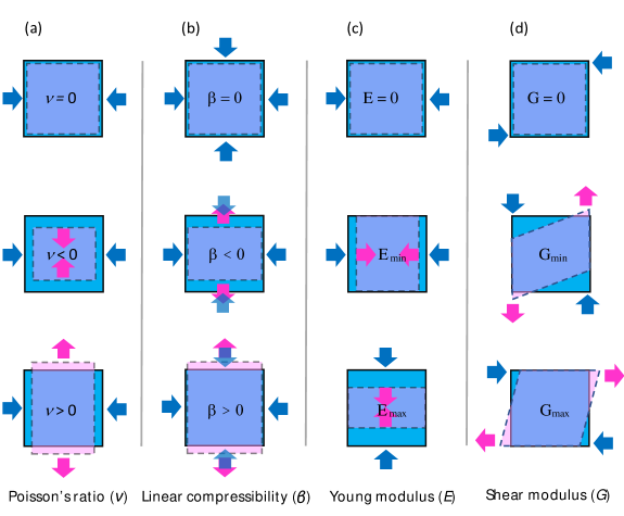
Figure 1: Schematic representation of the directional (a) Poisson’s ratio ($\nu$), (b) linear compressibility ($\beta$), (c) shear modulus (G), and (d) Young’s modulus (E). Blue arrows represent the direction of the stress exerted, and pink arrows the axis show along which the response is measured.

The present work’s primary motivation is to introduce a comprehensive and efficient program that accommodates all the features of these codes in one place, add some new features, and address their shortcomings. Table 1 compares ElATools features with ElAM, ELATE, and MechElastic. Note that other new features may be added in the updates of these packages in the future.

Table 1: Comparison of ElATools with the available primary tools for analyzing anisotropic elastic properties.

Features		MechElastic	ELAM	ELATE	ElATools
Main mechanical properties in 3D (see Appendix A )		✓	✓	✓	✓
Main mechanical properties in 2D		✓	✗	✗	✓
Hardness information		✓	✗	✗	✓
Elastic tensor eigenvalues in 3D		✓	✗	✓	✓
Elastic tensor eigenvalues in 2D		✓	✗	✗	✓
Visualization of the 3D surfaces in 3D materials	Shear modulus	✓	✓	✓	✓
	Poisson’s ratio	✓	✓	✓	✓
	Pugh ratio	✓	✗	✗	✓
	Linear compressibility	✓	✓	✓	✓
	Bulk modulus	✓	✗	✗	✓
	Young’s modulus	✓	✓	✓	✓
	Phase velocities	✗	✗	✗	✓
	Group velocities	✗	✗	✗	✓
	Power flow angles	✗	✗	✗	✓
	Minimum thermal conductivity	✗	✗	✗	✓
Visualization of the 2D projections on an arbitrary plane in 3D materials		✗	✗	✗	✓
Visualization of 2D polar covers in 2D materials	Shear modulus	✗	✗	✗	✓
	Poisson’s ratio	✗	✗	✗	✓
	Young’s modulus	✗	✗	✗	✓
Visualization of the 2D heat-map and polar heat-map in 3D and 2D materials		✗	✗	✗	✓
The database of elastic tensors (Materials Project’s database)	Offline	✗	✗	✗	✓
	Online	✓	✗	✓	✓
Various output formats for custom drawing or displaying with different software	VRLM format	✗	✓	✗	✓
	HTML (offline) format	✗	✗	✗	✓
	agr format	✗	✗	✗	✓
	gpi format	✗	✗	✗	✓
	dat format	✗	✗	✗	✓

The highlighted features of ElATools are as follows:

• Compute and display the main mechanical properties such as Young’s modulus, shear modulus, p-wave modulus, universal anisotropy index Ranganathan and Ostoja-Starzewski (2008a), Chung-Buessem anisotropy index Ranganathan and Ostoja-Starzewski (2008a), log-Euclidean anisotropy parameter Kube (2016), Kleinman’s parameter Kleinman (1962), Hardness information, Cauchy pressure, Poisson’s ratio, Pugh’s ratio, according to the three averaging schemes of Voigt, Reuss, and Hill Hill (1952) - Many of these features are included in ELAM, ELATE, and MechElastic codes.

• Investigation of mechanical stability using calculation of six (three) eigenvalues of the elastic tensor in 3D (2D) materials - This option exists only in ELATE (for 3D materials) and MechElastic (for 2D and 3D materials).

• Visualization of the 3D surfaces and 2D projections on any desired plane for shear modulus, Poisson’s ratio, Pugh ratio, linear compressibility, bulk modulus, and Young’s modulus. - ELATE and MechElastic only depict these features on XY, XZ, and ZY planes. Currently, visualization of the 3D surfaces and 2D projections on any desired plane for bulk modulus and Pugh ratio does not exist in either ELAM or ELATE.

• Visualization of the 3D surfaces and 2D projections on any desired plane for phase velocities, group velocities and power flow angles (includes primary, fast-secondary and slow-secondary modes) in 3D materials - These options do not exist in the ELAM and ELATE or MechElastic.

• Visualization of the 2D polar covers for Poisson’s ratio, shear modulus, and Young’s modulus in 2D materials - This option does not exist in the ELATE, MechElastic, and ELAM.

• An offline/online database of more than 13000 elastic tensors taken from Materials API (Materials Project database) - This option is also available online in ELATE and MechElastic.

• Supports various output formats for custom drawing or displaying with different software: “.dat” files for standard plotting, “.wrl” files for visualization of the 3D surfaces by view3dscene software Kamburelis and other Castle Game Engine developers (2020), “.agr” files for visualization of the 2D projections that are opened by XMGRACE Team (2008), “.html” files for visualization of the 3D surfaces by any Web browser, and “.gpi” script files for visualization of the 3D surfaces, 2D heat maps (for 3D materials), polar-heat maps (for 2D materials), and 2D projections that can be run by GNUPLOT Janert (2010) - ELAM generates only VRML (for 3D visualization) and PS formats (for 2D cut visualization). ELATE provides images online in PNG format only. MechElastic displays properties by matplotlib and pyvista python libraries.

• A user-friendly code with a terminal-based graphical user interface (GUI). A summary of this terminal-based GUI is included in Supplementary Information. - This feature does not exist in the ELAM and ELATE or MechElastic.

The rest of the paper is arranged as follows: The theoretical background of elasticity and analysis of elastic tensor is explained in detail in the next section. Package descriptions, including the workflow, code structure, installation, input and output files, visualization data, and test cases are presented in Sec. 3. Sec. 4 is summary and outlook. Finally, appendices A, B, C, D and Supplementary Information file are provided as complementary parts.

II Theoretical Background

II.1 Hooke’s law and elastic tensor of crystals

The shape of solid material changes when subjected to stress. Provided that the stress is below a specific value, the elastic limit, the strain is recoverable (Fig. 2).

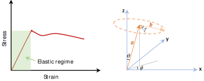
Figure 2: Schematic stress–strain curves and definitions of angles used to describe the directions in the calculations related to ElATools. The elastic regime corresponds to the portion of the diagram where the strain is proportional to the stress.

This means that the material returns to its original shape when the stress is removed. In this elastic regime, according to Hooke’s law, it can be stated that for sufficiently low stresses, the amount of strain is proportional to the magnitude of the applied stress:

$$\varepsilon=S\sigma,$$ (1)

where S is a constant. S is called the elastic compliance constant (ECC), or the compliance. Another form of this equation can be written as follows,

$$\varepsilon=C\sigma,\,\,\,E\equiv C=1/s,$$ (2)

where C is the elastic stiffness constant (ESC), or stiffness, and E is Young’s modulus. The general form of Hooke’s law can be rewritten in the form of tensor,

$$\varepsilon_{ij}=S_{ijkl}\sigma_{kl},$$ (3)

where S_ijkl are the ECCs of the crystal. Also, as an alternative to Eq.(2),

$$\sigma_{ij}=c_{ijkl}\varepsilon_{kl},$$ (4)

where C_ijkl are the ESCs. Eq.(3) and Eq.(4) stand for nine equations, each with nine terms on the right-hand side. The S_ijkl or C_ijkl are 4^th-rank tensors, and $\epsilon$_ij or $\sigma$_ij${}_{\ }$ are second^th-rank tensors. Hence, the C${}_{ijkl\ }$(S_ijkl) consists of 81 stiffness (compliances) constants of the crystal. Due to the inherent symmetries (translational and rotational symmetries) of $\epsilon$_ij, $\sigma$_ij, and S_ijkl or C${}_{ijkl,\ }$ the number of independent coordinates of the 4^th-rank tensor reduces to 21 for the least symmetric case. On the other hand, the further reduction resulting from the symmetry of the crystal can be applied to this number: 21 for triclinic, 15 for monoclinic, 9 for orthorhombic, 7 for trigonal, 5 for tetragonal, 5 for hexagonal and 3 for cubic.

II.2 Transformation law, Christoffel equation, and representation surfaces of elastic properties

A 4^th-rank tensor is defined (like tensors of lower rank) by its transformation law Nye et al. (1985). We know that the 81 tensor components $A_{\,ijkl}$ representing a physical quantity are said to form a 4^th-rank tensor if they transform on change of axes to $A^{\prime}_{\,ijkl}$, where

$$A^{\prime}_{\,ijkl}=a_{im}\,a_{jn}\,a_{ko}\,a_{lp}A_{mnop}.$$ (5)

It can be shown that 4^th-rank tensor S_ijkl or C_ijkl follows this rule Nye et al. (1985):

$$\left.\begin{array}[]{l}{\varepsilon^{\prime}_{ij}=a_{ik}a_{jl}\varepsilon_{kl},}\\ {\varepsilon_{kl}=S_{klmn}\sigma_{mn},}\\ {\sigma_{mn}=a_{om}a_{pn}\sigma^{\prime}_{op},}\end{array}\right\}\varepsilon^{\prime}_{ij}=a_{ik}a_{jl}\,S_{klmn}\,a_{om}a_{pn}\,\sigma^{\prime}_{op}.$$ (6)

By comparing Eq.(3) and the recent equation, we have:

$$S^{\prime}_{ijkl}=a_{im}a_{jn}a_{ko}a_{lp}S_{mnop}\,,$$ (7)

which is the necessary transformation law. To express the anisotropic form of Hooke’s law in matrix notation, we use the Voigt notation scheme. In the $S^{\prime}_{ijkl}$ and S_mnop, the first two suffixes are abbreviated into a single one running from 1 to 6, and the last two are abbreviated in the same way, according to the following Voigt scheme:

$$\begin{array}[]{l}{{\rm Tensor\;notation}:{\rm\;}11{\rm\;}\,\,22\,\,{\rm\;}33{\rm\;}\,\,23,32\,\,\,{\rm\;}31,13\,\,\,{\rm\;}12,21}\\ {{\rm Matrix\;notation}:{\rm\;}\,1{\rm\;}\,\,\,\,\,2{\rm\;}\,{\rm\;}\,\,\,3{\rm\;}\,\,\,\,\,\,\,4{\rm\;}\,\,\,\,\,\,\,\,\,\,\,\,\,5{\rm\;}\,\,\,\,\,\,\,\,\,\,\,6}\end{array}$$ (8)

Therefore, the components of the stress ($\sigma$) and the strain ($\epsilon$) tensors are written in a single suffix running from 1 to 6,

$$\begin{array}[]{l}{\sigma_{ij}=\left(\begin{array}[]{ccc}{\sigma_{11}}&{\sigma_{12}}&{\sigma_{13}}\\ {\sigma_{12}}&{\sigma_{22}}&{\sigma_{23}}\\ {\sigma_{13}}&{\sigma_{23}}&{\sigma_{33}}\end{array}\right)\stackrel{{\scriptstyle{\rm Voigt}\,\,{\rm scheme}}}{{\longrightarrow}}\left(\begin{array}[]{ccc}{\sigma_{1}}&{\sigma_{6}}&{\sigma_{5}}\\ {\sigma_{6}}&{\sigma_{2}}&{\sigma_{4}}\\ {\sigma_{5}}&{\sigma_{4}}&{\sigma_{3}}\end{array}\right),}\\ \\ {\varepsilon_{ij}=\left(\begin{array}[]{ccc}{\varepsilon_{11}}&{\varepsilon_{12}}&{\varepsilon_{13}}\\ {\varepsilon_{12}}&{\varepsilon_{22}}&{\varepsilon_{23}}\\ {\varepsilon_{13}}&{\varepsilon_{23}}&{\varepsilon_{33}}\end{array}\right)\stackrel{{\scriptstyle{\rm Voigt}\,\,{\rm scheme}}}{{\longrightarrow}}\left(\begin{array}[]{ccc}{\varepsilon_{1}}&{{\textstyle\frac{1}{2}}\varepsilon_{6}}&{{\textstyle\frac{1}{2}}\varepsilon_{5}}\\ {{\textstyle\frac{1}{2}}\varepsilon_{6}}&{\varepsilon_{2}}&{{\textstyle\frac{1}{2}}\varepsilon_{4}}\\ {{\textstyle\frac{1}{2}}\varepsilon_{5}}&{{\textstyle\frac{1}{2}}\varepsilon_{4}}&{\varepsilon_{3}}\end{array}\right).}\end{array}$$ (9)

According to this scheme, we have for the S_mnop${}_{\ }$Nye et al. (1985),

S${}_{mnop\ }$= S_ij, when i and j are 1; 2 or 3,

2S_mnop = S_ij, when either i or j are 4; 5 or 6,

4S_mnop = S${}_{ij\ }$when both i and j are 4; 5; or 6.

Therefore, Eq.(3) takes the shorter form:

$$\varepsilon_{i}=S_{ij}\sigma_{j}\,\,\,\,(i,j=1,{\rm\;}2,...,{\rm\;}6).$$ (10)

The Voigt scheme replaces the cumbersome 2^th and 4^th-rank tensors in a 3-dimensional vector space of vectors and matrices in a 6-dimensional vector space. The reason for introducing the factors of 0.5 in Eq.(9) and the factors of 2 and 4 into the definitions of the S_ij is to enable writing Eq.(10) in a compact form.

Using S_ij in Eq.(10) and Eq.(5), we can get a general and and straightforward compliance transformation relation for any crystal from the old systems (${T^{\prime}}$) to measurement systems (T):

$$T^{\prime}_{\,ijkl}=r_{i\alpha}\,r_{j\beta}\,r_{k\gamma}\,r_{l\delta}T_{\alpha\beta\gamma\delta},$$ (11)

where the r represents the components of the rotation matrix (or direction cosines). In general, the tension produces not only longitudinal, and lateral strains, but shear strains as well. Therefore, spherical coordinates are suitable for such stresses and the responses that materials give to stresses. We choose r$\mathrm{\equiv}$a to be the first unit vector in the new basis set Marmier et al. (2010); Gaillac et al. (2016); Nordmann et al. (2018),

$$\textbf{{a}}=\left(\begin{array}[]{c}{\sin(\theta)\cos(\varphi)}\\ {\sin(\theta)\sin(\varphi)}\\ {\cos(\theta)}\end{array}\right);\,\,\,\,\,\,\,0\,\leq\theta\leq\pi,\,\,\,0\leq\varphi\leq\pi,$$ (12)

This unit vector (a) is required to determine Young’s modulus (E), linear compressibility ($\beta$), and bulk modulus (B). But some elastic properties such as the shear modulus (G) and Poisson’s ratio (v) requires another perpendicular direction. Therefore, we define unit vector b, which is perpendicular to a (see Fig. 2), as follows Marmier et al. (2010); Gaillac et al. (2016):

$$\textbf{{b}}\equiv\left(\begin{array}[]{c}{\cos(\theta)\cos(\varphi)\cos(\gamma)-\sin(\theta)\sin(\gamma)}\\ {\cos(\theta)\sin(\varphi)\cos(\gamma)-\cos(\theta)\sin(\gamma)}\\ {-\sin(\theta)\cos(\gamma)}\end{array}\right),\,\,\,\,0\leq\,\gamma\leq 2\pi.\,0$$ (13)

Therefore, by defining these two vectors, Eq.(11) is as follows:

$$T^{\prime}_{\,\alpha\beta\gamma\delta}=a_{\alpha i}\,a_{\beta j}\,b_{\gamma k}\,b_{\delta l}T_{ijkl},$$ (14)

Using this equation, we can calculate the representation surfaces for elastic properties. For instance, from Eq.(10), we know that Young’s modulus can be obtained by using purely normal stress (see Fig. 1(c)),

$$\begin{array}[]{l}{E(\textbf{a})\equiv\frac{1}{S^{\prime}_{1111}}=\sum_{ijkl}^{6}\frac{1}{a_{1i}a_{1j}a_{1k}a_{1l}S_{ijkl}}}\\ \\ \,\,\,\,\,\,\,\,\,\,\,\,\,\,\,\,\,\,\,\,\,\,\,\,\,\,\,\,\,\,\,\,\ =\frac{1}{S^{\prime}_{11}}=\frac{1}{a_{i}a_{j}a_{k}a_{l}S_{ijkl}}\,\,\,\,({\rm by}\,{\rm Einstein{{}^{\prime}}s\;summation\;rule}),\end{array}$$ (15)

The volume compressibility of a crystal is the proportional decrease in volume of a crystal when subjected to unit hydrostatic pressure, but the linear compressibility is the relative decrease in length of a line when the crystal is subjected to unit hydrostatic pressure (HP). Hence, it is obtained by applying isotropic stress (P_HP) in a tensor form so that $\varepsilon$_ij=-(P_HP)S_ijkk Marmier et al. (2010); Nye et al. (1985), and by considering that the extension in a direction is $\varepsilon$_ija_ia_j, and for this reason, we have:

$$\beta(\textbf{{a}})=a_{i}a_{j}a_{k}a_{k}S_{ijkk}=a_{i}a_{j}S_{ijkk}\,;\,\,\,a_{k}.\,a_{k}=1$$ (16)

On the other hand, the relationship between $\beta$ and B can be expressed as follows Nye et al. (1985),

$$B(\textbf{{a}})=\frac{1}{\beta(\textbf{a})}=\frac{1}{a_{i}a_{j}S_{ijkk}}$$ (17)

As mentioned, the G and $\nu$ are not as straightforward to represent and depend on two directions (a and b). The shear ratio (Poisson’s ratio) is obtained by applying a pure shear (Fig. 1(d)) (a purely normal) stress in the vector form of Eq.(3), and results in:

$$G(\textbf{{a}},\textbf{{b}})=\frac{1}{4S_{1212}}=\frac{1}{4S_{66}}=\frac{1}{4}\frac{1}{a_{i}b_{j}a_{k}b_{l}S_{ijkl}},$$ (18)

$$\nu(\textbf{{a}},\textbf{{b}})=-\frac{S^{\prime}_{1212}}{S^{\prime}_{1111}}=-\frac{S^{\prime}_{12}}{S^{\prime}_{11}}=-\frac{a_{i}a_{j}b_{k}b_{l}S_{ijkl}}{a_{i}a_{j}a_{k}a_{l}S_{ijkl}}.$$ (19)

To better understand these equations, we obtain Young’s modulus of a cubic crystal. As for cubic crystal, because of lattice symmetry, there are three independent variables C₁₁, C₁₂, C₄₄ in the C_ij, and S₁₁, S_12, and S₃₃ in the S_ij. Using Eq.(15) and Eq.(12), we have:

$$\begin{array}[]{l}{S^{\prime}_{1111}=a_{11}a_{11}a_{11}a_{11}S_{1111}+a_{12}a_{12}a_{12}a_{12}S_{2222}+a_{13}a_{13}a_{13}a_{13}S_{3333}+}\\ \\ {\,\,\,\,\,\,\,\,\,\,\,\,\,\,\,\,\,\,\,\,a_{11}a_{11}a_{12}a_{12}S_{1122}+a_{11}a_{11}a_{13}a_{13}S_{1133}+a_{12}a_{12}a_{13}a_{13}S_{2233}+}\\ \\ {\,\,\,\,\,\,\,\,\,\,\,\,\,\,\,\,\,\,\,\,a_{11}a_{11}a_{12}a_{12}S_{2211}+a_{11}a_{11}a_{13}a_{13}S_{3311}+a_{12}a_{12}a_{13}a_{13}S_{3322}+}\\ \\ {\,\,\,\,\,\,\,\,\,\,\,\,\,\,\,\,\,\,\,\frac{1}{4}[a_{12}a_{13}a_{12}a_{13}S_{2323}]+\frac{1}{4}[a_{13}a_{11}a_{13}a_{11}S_{3131}]+\frac{1}{4}[a_{11}a_{12}a_{11}a_{12}S_{1212}]}\\ \\ {\,\,\,\,\,\,\,\,\,\,\,\,\,\,=S_{11}(a_{11}^{4}+a_{12}^{4}+a_{13}^{4})+(\frac{1}{4}S_{44}+2S_{12})[a_{12}^{2}a_{13}^{2}+a_{11}^{2}a_{13}^{2}+a_{11}^{2}a_{12}^{2}],}\end{array}$$ (20)

with further simplification,

$$\frac{1}{E}=S^{\prime}_{1111}=S_{11}-2(S_{11}-S_{12}-\frac{1}{2}S_{44})(a_{11}^{2}a_{12}^{2}+a_{11}^{2}a_{13}^{2}+a_{12}^{2}a_{13}^{2})$$ (21)

To calculate the orientation-dependent Poisson’s ratio, shear modulus and Young’s modulus in 2D material, Eq.(12) and Eq.(13) are used again and changed as follows:

$$\textbf{a}=\left(\begin{array}[]{c}{\cos(\varphi)}\\ {\sin(\varphi)}\\ {0}\end{array}\right);\,\,\,\textbf{b}=\left(\begin{array}[]{c}{-\sin(\varphi)}\\ {\cos(\varphi)}\\ {0}\end{array}\right)\,;\,\,\,\,\,\,\,\,0\leq\varphi\leq 2\pi.\,$$ (22)

For 2D system, according to Hooke’s law (Eq.(3) and Eq.(4)), the relationship between $\sigma$ and the corresponding strain tensor $\varepsilon$ can be described using the stiffness tensor C_ij, for orthogonal symmetry under plane stress conditions as Zhao et al. (2016),

$$\left(\begin{array}[]{c}{\sigma_{11}}\\ {\sigma_{22}}\\ {\sigma_{12}}\end{array}\right)=\left(\begin{array}[]{ccc}{C_{11}}&{C_{12}}&{0}\\ {C_{12}}&{C_{22}}&{0}\\ {0}&{0}&{C_{66}}\end{array}\right)\left(\begin{array}[]{c}{\varepsilon_{11}}\\ {\varepsilon_{22}}\\ {2\varepsilon_{12}}\end{array}\right),$$ (23)

where Voigt notation has been used for C_ij. Here C${}_{11\ }$(S₁₁), C${}_{22\ }$(S₂₂), C₁₂=C${}_{21\ }$(S₁₂=S₂₁), and C${}_{66\ }$(S₆₆) represent C${}_{1111\ }$(S₁₁₁₁), C${}_{2222\ }$(S₂₂₂₂), C${}_{1122\ }$(S₁₁₂₂), and C${}_{1212\ }$(S₁₂₁₂), respectively. So, using the previous equations, the in-plane Young’s modulus, shear modulus, and Poisson’s ratio can be defined as:

$${E(\varphi)=\frac{1}{S_{11}\cos^{4}(\varphi)+S_{22}\sin^{4}(\varphi)+(2S_{12}+S_{66})\cos^{2}(\varphi)\sin^{2}(\varphi)}},$$ (24)

$$\nu(\varphi)=-\frac{[S_{11}-S_{66}+S_{22}]\cos^{2}(\varphi)\sin^{2}(\varphi)+S_{12}\cos^{4}(\varphi)+S_{12}\sin^{4}(\varphi)}{[2S_{12}+S_{66}]\cos^{2}(\varphi)\sin^{2}(\varphi)+S_{11}\cos^{4}(\varphi)+S_{22}\sin^{4}(\varphi)},$$ (25)

$$\frac{1}{4G(\varphi)}=[S_{11}+S_{22}-2S_{12}]\cos^{2}(\varphi)\sin^{2}(\varphi)+\frac{1}{4}S_{66}[\cos^{4}(\varphi)+\sin^{4}(\varphi)-2\sin^{2}(\varphi)\cos^{2}(\varphi)].$$ (26)

Equations (24),(25), and (26) can be used for hexagonal, square, and rectangular 2D crystal systems (see Fig. 3), which have two, three, and four independent elastic constants, respectively. For two-dimensional oblique systems, there are six independent elastic constants(C₁₆ and C₂₆ are non-zero). In this case, the above equations are defined as follows Jasiukiewicz et al. (2008, 2010):

$$\centering\begin{split}E(\varphi)=\frac{1}{S_{11}\cos^{4}(\varphi)+S_{22}\sin^{4}(\varphi)+(2S_{12}+S_{66})\cos^{2}(\varphi)\sin^{2}(\varphi)+}\\ \frac{1}{2S_{16}\cos^{3}(\varphi)\sin(\varphi)+2S_{26}\sin^{3}(\varphi)\cos(\varphi))},\end{split}\@add@centering$$ (27)

$$\centering\begin{split}\nu(\varphi)=-\frac{[S_{22}-S_{66}+S_{22}]\cos^{2}(\varphi)\sin^{2}(\varphi)+S_{12}[\cos^{4}(\varphi)+\sin^{4}(\varphi)]+}{[2S_{12}+S_{66}]\cos^{2}(\varphi)\sin^{2}(\varphi)+S_{11}\cos^{4}(\varphi)+S_{22}\sin^{4}(\varphi)+}\\ \frac{S_{16}[\sin^{3}(\varphi)\cos(\varphi)-\cos^{3}(\varphi)\sin(\varphi)]+}{2S_{16}\sin^{3}(\varphi)\cos(\varphi)+}\\ \frac{S_{26}[\cos^{3}(\varphi)\sin(\varphi)-\sin^{3}(\varphi)\cos(\varphi)]}{2S_{26}\cos^{3}(\varphi)\sin(\varphi)},\end{split}\@add@centering$$ (28)

$$\centering\begin{split}{\frac{1}{4G(\varphi)}=[S_{11}+S_{22}-2S_{12}]\cos^{2}(\varphi)\sin^{2}(\varphi)+\frac{1}{4}S_{66}[\cos^{4}(\varphi)+\sin^{4}(\varphi)-2\sin^{2}(\varphi)\cos^{2}(\varphi)]}\\ {+S_{16}[\sin^{3}(\varphi)\cos(\varphi)-\cos^{3}(\varphi)\sin(\varphi)]+S_{26}[\cos^{3}(\varphi)\sin(\varphi)-\sin^{3}(\varphi)\cos(\varphi)]}.\end{split}\@add@centering$$ (29)

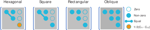
Figure 3: Classification of crystal systems and independent elastic constants for 2D materials.

An important relation in material science is the connection between the elastic constants tensor and elastic wave velocities of a solid. Since sound is a form of elastic waves traveling in a homogeneous medium (e.g., a perfect crystal), the C_ijkl will contain information about how these sound waves are propagated. Knowing the elastic constants makes it possible to predict the sound velocities in a material by the Christoffel equation Auld and Fields (1990); Koos and Wolfe (1984), and determining the dispersion relation for these waves is possible by solving this equation:

$$[M_{il}-\rho\omega^{2}\delta_{il}]s_{l}=0.$$ (30)

For a plane wave with wave vector q, frequency $\omega$, and polarization $\hat{s}$ in a material with density $\rho$, the Christoffel matrix ($M_{il}$) can be defined as follows:

$$M_{il}=q_{j}C_{ijkl}q_{k}.$$ (31)

Eq.(30) is a simple eigenvalue problem that can be routinely solved for arbitrary q, and the result is a set of three frequencies and polarization vectors for each value of q. The Christoffel matrix is symmetric and real; so the eigenvalues are real, and polarization vectors {$\hat{\textbf{s}}$} constitute an orthogonal basis.

We use the reduced elastic constants tensor $\tilde{C}_{ijkl}$ = $\rho^{-1}$C_ijkl and the corresponding reduced Christoffel matrix ($\tilde{M}_{il}$) for further simplification. Due to the wavelength-independence of the velocities, we do not consider q a dimension of inverse length but a dimensionless unit vector that defines only the direction of travel of a plane wave. This causes the dimension of the $\tilde{M}_{il}$ to change from frequency to velocity squared. Therefore, Eq.(30) can be reduced as follows:

$$[\tilde{M}_{il}-v^{2}_{p}\delta_{il}]s_{l}=0;\,\,v^{2}_{p}=\omega^{2}/q^{2},$$ (32)

where $v_{p}$ is the velocity of a plane wave traveling in the direction of $\hat{q}$. The calculations of a material sound velocities based on the Eq.(32) are a straightforward eigenvalue problem. From this equation, we obtain three velocities, one primary (P) and two secondary (S), which correspond to the longitudinal and transversal polarizations, respectively. Generally, the velocity of a plane wave is referred to as the phase velocity ($v_{p}$). The real sound, like $v_{p}$ is never purely monochromatic nor purely planar. Hence, we consider a wave packet with a small spread in wavelength and direction of travel. The velocity of the wave packet formed by the superposition of these phase waves is called the group velocity ($v_{g}$).It is the velocity that acoustic energy travels through a non-dispersive and homogeneous medium and is defined by

$$\mathbf{v}_{g}\equiv\mathbf{\nabla}v_{p},$$ (33)

where $v_{p}$ is a scalar function of $\hat{\textbf{q}}$, and $\textbf{v}_{g}$ is a vector-valued function, which generally does not lie in the direction of $\hat{q}$. The angle between $v_{p}$ and $v_{g}$ is called the power flow angle ($\psi$) and is defined as

$$\nu_{p}=\nu_{g}cos(\psi);cos(\psi)=\mathbf{\hat{n}}_{p}.\mathbf{\hat{n}}_{g},$$ (34)

where $\hat{\textbf{n}}_{p}$ and $\hat{\textbf{n}}_{g}$ are the normalized directions of the $v_{p}$ and $v_{g}$, respectively.

II.3 Mechanical properties and elastic anisotropy of 2D and 3D materials

From elastic constants, other basic elastic properties, including elastic moduli, can be obtained. The elastic response of an isotropic system is generally described by the B and the G, which may be obtained by averaging the single-crystal elastic constants. The averaging methods most often used are the Voigt Voigt et al. (1928), Reuss Reuss (1929) and Hill Hill (1952) bounds. In Voigt’s and, Reuss’s approximations, the equation takes the following form:

$$\begin{array}[]{l}{B_{V}=9^{-1}([C_{11}+C_{22}+C_{33}]+2[C_{12}+C_{23}+C_{31}]),}\\ \\ {G_{V}=15^{-1}([C_{11}+C_{22}+C_{33}]-[C_{12}+C_{23}+C_{13}]+3[C_{44}+C_{55}+C_{66}]),}\\ \\ {B_{R}=([S_{11}+S_{22}+S_{33}]+2[S_{12}+S_{23}+S_{13}])^{-1},}\\ \\ {G_{R}=15(4[S_{11}+S_{22}+S_{33}]-4[S_{12}+S_{23}+S_{31}]+3[S_{44}+S_{55}+S_{66}])^{-1}.}\end{array}$$ (35)

Also, the arithmetic mean of the Voigt and Reuss bounds, termed the Voigt-Reuss-Hill (VRH) average is also found as a better approximation to the actual elastic behavior of a polycrystal material,

$$\begin{array}[]{l}{B_{VRH}=\frac{1}{2}(B_{V}+B_{R}),}\\ \\ {G_{VRH}=\frac{1}{2}(G_{V}+G_{R})}\end{array}$$ (36)

The Young’s modulus (E), and Poisson’s ratio ($\nu$) for an isotropic material are given by:

$$E=\frac{9BG}{3B+G},\,\,\,\,v=\frac{3B-2G}{2(3B+G)}.$$ (37)

The elastic anisotropy is a crucial measurement of the anisotropy of chemical bonding and can be calculated by elastic constants. For all crystal systems, the bulk response is in general, anisotropic, and one must account for such contributions to quantify the extent of anisotropy accurately. For this purpose, Ranganathan et al. Ranganathan and Ostoja-Starzewski (2008a) introduce a new universal anisotropy index (A^U),

$$A^{U}=5\frac{G_{V}}{G_{R}}+\frac{B_{V}}{B_{R}}-6.$$ (38)

It is noteworthy that in weakly anisotropic materials, i.e. isotropic material, all such averages lead to similar results for elastic moduli. The mechanical behavior such as ductile or brittle can be represented by the ratio of the G to the B, i.e., the Pugh ratio G/B, by simply considering B as the resistance to fracture and G as the resistance to plastic deformation. The critical value of the Pugh ratio to separate ductile and brittle materials is around 0.57. If G/B $\mathrm{<}$ 0.57, the material is more ductile; otherwise, it behaves in a brittle manner Saeidi et al. (2019a); Pugh (1954). Hence, a higher Pugh ratio indicates more brittleness property. Cauchy pressure (P_C) is another characteristic to describe the brittleness and ductility of the metals and compounds and is defined in different symmetries Pettifor (1992); Qu et al. (2020); Duan et al. (2021) by:

$$P_{C}^{c}=C_{12}-C_{44}\,\ (Cubic\,\,symmetry)$$ (39)

$$P_{C}^{a}=C_{13}-C_{44},P_{C}^{b}=C_{12}-C_{66}\,\ (Hexagonal,Trigonal,Tetragonal\,\,symmetries)$$ (40)

$$P_{C}^{a}=C_{23}-C_{44},P_{C}^{b}=C_{13}-C_{55},P_{C}^{c}=C_{12}-C_{66}\,\ (Orthorhombic\,\,symmetry)$$ (41)

For covalent materials with brittle atomic bonds, the P_C is negative, because in this case, material resistance to shear strain, i.e., C₄₄, is much more than that for volume change, i.e., C₁₂ (for cubic symmetry). However, the P_C must be positive for the metallic-like bonding, where the electrons are almost delocalized. For an isotropic crystal, A^U is zero. The departure of A^U from zero defines the extent of the elastic anisotropy. In addition to these properties, Appendix A provides a complete list of various parameters and moduli related to the elastic and mechanical properties of materials that ElATools is able to calculate.

In this work, the relation among the E, G, v, and elastic stiffness constants for a 2D system are derived as,

$$\centering\begin{split}{E_{x}=\frac{C_{11}C_{22}-C_{12}C_{21}}{C_{22}},}\\ {E_{y}=\frac{C_{11}C_{22}-C_{12}C_{21}}{C_{11}},}\\ {G_{xy}=C_{66},}\\ {\,v_{xy}=\frac{C_{21}}{C_{22},},v_{yx}=\frac{C_{12}}{C_{11}},}\\ \end{split}\@add@centering$$ (42)

where E_l= $\sigma$_l/$\varepsilon$_l is Young’s modulus along the axis of l. v_lk =-d$\varepsilon$_k/d$\varepsilon$_l is the Poisson’s ratio with tensile strain applied in the l direction and the response strain in the k direction. G_xy is the shear modulus in the xy-plane.

III Software description and Features

III.1 Workflow and structure of ElATools

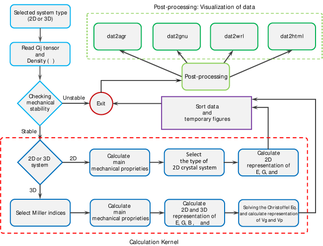
Figure 4: The flowchart of ElATools. The red dashed line represents the Calculation Kernel (CK) block. The green dashed line represents the post-processing stage.

The simple workflow of the ElATools package is illustrated in Fig. 4. First, the type of either 2D or 3D material is chosen to determine the calculations in the Calculation Kernel (CK) block. Then, ElATools reads the C_ij data as an input file. At this point, C_ij data can be extracted from the output files of IRelast Jamal et al. (2018), IRelast2D Boochani et al. (2019), Elast Blaha et al. (2020), AELAS Zhang and Zhang (2017), and ElaStic Golesorkhtabar et al. (2013) packages. The output files of these packages are supported as input files by ElATools (see Sec. 3.3). As mentioned earlier, for 3D materials, ElATools has an offline/online database of more than 13000 elastic tensors taken from Materials API (Materials Project database). The user can enter the next steps of calculating ElATools by entering the Materials API-ID of the structure. The developers of ElATools intend to keep the elastic tensors database updated according to the latest release of the Materials Project database. Subsequently, the C_ij tensor enters the mechanical stability check stage. There are four methods of the Born elastic stability conditions for a crystal, which are valid regardless of the crystal symmetry: 1) if the second-order elastic stiffness tensor C_ij is definitely positive, 2) if all eigenvalues of C_ij are positive, 3) if all the leading principal minors of C_ij are positive, and 4) if an arbitrary set of minors of C_ij are all positive. Method (2) is used in the ElATools. If the stability conditions are satisfied, the tensor will enter the CK block; otherwise, the program will stop by showing a mechanical instability error.

In the CK block, the calculations are divided into two branches. If the system is 2D the main mechanical properties such as E_x, E_y, G_xy, v_xv, v_yx, etc. are determined, and then enter the orientation-dependent (OD) calculation step. At this stage, according to the equations of Sec. 2.2, OD of Young’s modulus, shear modulus, and Poisson’s ratio in the (001) plane are calculated. Also, in the (001) plane, the maximum and minimum values for these proprieties are calculated. For the 3D system, the process is like a 2D system. First, ElATools reads the hkl-index plane (e.g. (100)) entered by the user. Then, the polycrystalline Young’s modulus, bulk modulus, shear modulus, P-wave modulus, Poisson’s ratio, and Pugh ratio are calculated using three averaging approaches of Voigt, Reuss and Hill approximations. Besides anisotropy indices, Cauchy pressures and hardness information are determined. Subsequently, we arrive at the spatial dependence (SD) calculation process. The SD and the 2D projection of Young’s modulus, bulk modulus, shear modulus, Poisson’s ratio, and linear compressibility are calculated. To calculate the elastic waves properties such as phase and group velocities, ElATools can solve the Christoffel equation at the user’s request. Then, similar to the previous steps, it enters the spatial calculation process, and SD and the 2D projection of the phase and group velocities (primary and two secondary modes) are calculated.

Finally, the calculations obtained from these two branches are sorted and saved. The main mechanical properties are sorted in DATA.out. ElATools creates two directories named DatFile-hkl and PicFile-hkl, and stores files in “dat” format, and temporary figures of the properties in these directories, respectively. Temporary figures help us get an overview of the properties. Then, we enter the post-processing for visualization of the 3D spherical plot and their 2D projections with higher quality and detail.

There are four plugins for visualizing data in the post-processing stage: dat2gnu.x, dat2agr.x, dat2wrl.x, dat2html.x. The dat2gnu.x and dat2agr.x generate files for 2D graphical representations of elastic properties in “gpi” and “agr” formats, respectively, which can be run by GNUPLOT and XMGRACE programs. The dat2wrl.x and dat2html.x are also prepared for 3D graphical representations of elastic properties, capable of producing files in “wrl” and “html” formats. The wrl format can be visualized and explored with a VRML capable browser, such as View3dscene Kamburelis and other Castle Game Engine developers (2020). For HTML format can also be used from any Web browser. JavaScript written in this format uses plotly.js Sievert (2020), a free and recently open-sourced graphing library. We can represent dynamic parametric surfaces with these formats, making the spatial representation of mechanical properties more straightforward and fully interactive.

III.2 Installation and Requirements

The ElATools is written in Fortran90 and is installed with Intel Fortran (ifort) or GNU Fortran (gfortran) compiler. Before installing ElATools, the following libraries and packages should be installed: GNUPLOT, and LAPACK (Linear Algebra Package). LAPACK libraries are for numerical calculations and are used to calculate elastic compliance constant and so on. GNUPLOT is also used to plot temporary figures and the post-processing stages. One of the packages IRelast, Elast, AELAS, and ElaStic can calculate the elastic stiffness constant (C_ij). ElATools supports the output of these packages.

The ElATools is distributed in a compressed tar file elatools_1.**.tar.gz, which uncompresses into several directories: soc, doc, db, and bin. The soc directory contains the f90 files and Makefile. For the compilation, the Makefile must be modified for one’s system. The doc directory contains a copy of the short user guide and the examples directory. The db directory contains the elastic constant database files. The path of these files must be specified before installation. More details are provided in the short user guide. After installation, the executable files (Elatools.x, dat2gnu.x, dat2agr.x, dat2html.x, and dat2wrl.x) are saved in the bin directory. Finally, the code will run by executing Elatools.x.

III.3 Input and Output files

The only input data for ElATools is the elastic stiffness constant, which can be calculated by other packages. However, ElATools also supports output files of many packages for convenience, such as IRelast (or IRelast2D) with INVELC-matrix output file, Elast with elast.output output file, AELAS with ELADAT output file, ElaStic with ElaStic_2nd.out output file, and Cij.dat (3D system) or Cij-2D.dat (2D system) file for any other outputs (See Appendix B for more details). Several output files are generated in each run:

• Spatial-dependence and 2D projection files in 3D materials.

  For this case, fifteen files 3d_pro.dat (pro=bulk, young, poisson, comp, shear, pp, pf, ps, gp, gf, gs, pfp, pff, pfs, km) are generated. Among these files, the 3d_poisson.dat file includes the maximum value, minimum positive value, minimum negative value, and average value of Poisson’s ratio. The 3d_shear.dat file contains the maximum positive value, minimum positive value, and average value of shear modulus, and the 3d_comp.dat file also contains the positive and negative value of linear compressibility. Also, for 2D projection of any plane, nine files 2dcut_pro.dat (pro=bulk, young, poisson, comp , shear, km, gveloc, pveloc, and pfaveloc) are generated. It should be noted that 2dcut_p/g/pfveloc.dat files include primary, fast secondary, and slow secondary modes. See Table 3 for more details on 3d_pro.dat and 2dcut_pro.dat files.

• Orientation-dependent files in 2D materials.

  In this case, three files pro (pro= young, poisson, shear) are generated. Also, the poisson_2d_sys.dat file contains the maximum value, the minimum positive value, and the minimum negative value of Poisson’s ratio.

• DATA.dat file.

  This file contains the C_ij, S_ij, the main properties and the minimal and maximal values of Young’s modulus, bulk modulus, shear modulus, Poisson’s ratio, linear compressibility, power flow angle, phase, and group velocities as well as, the angles and directions along which these extrema occur.

• Temporary files.

  These files are used for post-processing.

III.4 Visualization and Post-processing

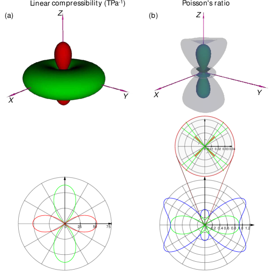
Figure 5: (a) The spatial-dependence and (b) 2D projection in (110) plane of linear compressibility and Poisson’s ratio of ZnAu₂(CN)₄ structure.

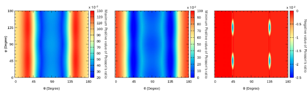
Figure 6: Poisson’s ratio heat maps with respect to $\theta$ and $\phi$ angles for ZnAu₂(CN)₄ compound. (a) Maximum positive values, (b) minimum positive values, and (c) negative values of Poisson’s ratio.

In the post-processing, three powerful tools dat2gnu.x, dat2agr.x, dat2wrl.x, and dat2html.x are designed to visualize of results, with output files in gpi, agr, wrl, and html formats, respectively. In Figs. 5–14, we show the corresponding plots for ZnAu₂(CN)₄ (space group P6222) Gupta et al. (2017), CrB₂ (space group P6/mmm) Chong et al. (2014), GaAs (space group F-43m) Auld (1973), (space group C2/m) Haastrup et al. (2018), $\delta$-phosphorene (space group Pmc21), and Pd₂O₆Se₂ (monolayer) structures Wang et al. (2017) by these three postprocessing tools and GNUPLOT, XMGRACE and view3dscene programs. In the following section, these three structures are examined. A list of the main elastic properties and anisotropy indices of ZnAu₂(CN)₄, CrB₂, GaAs, $\delta$-phosphorene ($\delta$-P), and Pd₂O₆Se₂ monolayer are given in Appendix C.

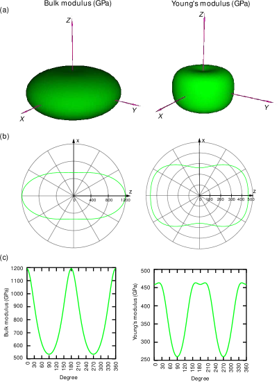
Figure 7: (a) The spatial-dependent and 2D projection in (b) polar and (c) cartesian coordinates in (110) plane of Poisson’s ratio and linear compressibility of the CrB₂ structure.

Test case (1): ZnAu₂(CN)₄. Fig. 5 shows the spatial-dependence and 2D projection in (110) plane of Poisson’s ratio and linear compressibility of ZnAu₂(CN)₄ structure. The negative linear compressibility for this compound is shown in Fig. 5(a). In these Figs., directions corresponding to positive values of linear compressibility are plotted in green, and those of NLC are plotted in red. The NCL of ZnAu₂(CN)₄ was predicted in Ref. Gupta et al. (2017), which is evident in the z-direction. The spatial-dependence and 2D projection in (110) plane of Poisson’s ratio are shown in Fig. 5(b). For Poisson’s ratio, which can be negative in some directions, three categories of colors are considered: directions corresponding to maximum (minimum) positive values of Poisson’s ratio are plotted in translucent blue (green) color, and those of NPR are plotted in red color. Calculations of ElATools based on the elastic tensor in Ref. Gupta et al. (2017) show that this structure, in addition to the NLC has a small NPR (-0.02) on (110) plane. Using GNUPLOT and dat2gnu.x tools, heat maps with respect to $\theta$ and $\phi$ angles are shown in Fig. 6. These 2D heat maps show the changes in the Poisson’s ratio relative to $\theta$ and $\phi$ angles in spherical space. NPR is well visible in the Fig. 6(c). For comparison, ELATE display the NPR feature due to the unavailability 2D representation in (110) plane (it can display only on three planes (100), (010), and (001)). Hence, the ability to select a custom plane is a unique feature in ElATools.

Test case (2): CrB₂. CrB₂ compound is investigated to evaluate ElATools and post-processing. Elastic tensor is taken from the calculations of Ref. Chong et al. (2014). The Young’s modulus and bulk modulus are shown in 3D and 2D ((010) plane) in Fig. 7. The spatial dependent files are generated by the dat2wrl.x and represented by the View3dscene programs (Fig.  7(a)). The orientation-dependent files in polar (Cartesian) coordinate are generated by dat2gnu.x (dat2agr.x) and displayed by GNUPLOT (XMGRACE) (see Fig.7(b) and (c)). For an isotropic system, in the spatial-dependence (polar and cartesian coordinates), the graph would be a sphere (a circle and a straight line). Fig. 7(a) shows that the bulk modulus and Young’s modulus of CrB₂ have anisotropy. The projections on the (010) plane show more details about the anisotropic properties of the bulk modulus and Young’s modulus.

Test case (3): GaAs. We employ gallium arsenide (GaAs) as an example to illustrate the capabilities of ElaTools, and the output figures will be briefly commented on here. In this example, we investigate the elastic wave properties of this compound. The values of $C_{ij}$ and $\rho$ were taken from Ref. Auld (1973). In Figs. 12 and 13, phase and group velocities for primary, fast, and slow secondary modes are calculated by Elatools and obtained by the dat2html.x (using plotly.js), dat2gnu.x (using Gnuplot) post-processing codes. In Figs. 8 and 9 it is clear that the distinction between fast secondary (FS) and slow secondary (SS) modes always refers to the phase velocity since the group velocity of the FS mode could be lower than that of the SS mode for certain propagation directions. According to Table 10 and these Figures, the minimum and maximum anisotropy are associated with primary (P) and SS modes, respectively. In Figs. 8(a) and 9(a), the P modes are not spherical, and their anisotropy is higher than the other modes. Also, as shown in Figs. 8(c) and 9(c), the P modes propagation patterns are more complex, indicating higher anisotropy than other modes.

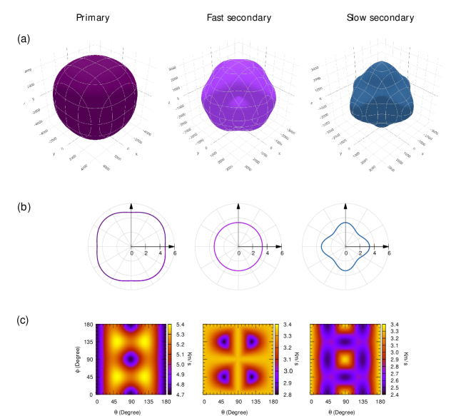
Figure 8: (a) The spatial-dependent, (b) 2D projection in polar coordinates on (100) plane, and (c) heat maps of phase velocity ($\nu_{p}$) for primary, fast, and slow secondary modes of the GaAs compound.

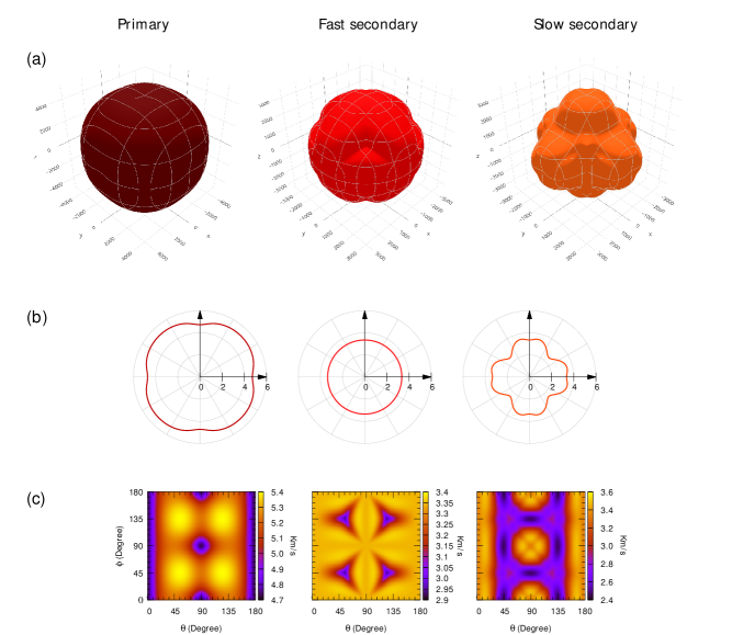
Figure 9: (a) The spatial-dependent, (b) 2D projection in polar coordinates on (100) plane, and (c) heat maps of group velocity ($\nu_{g}$) for primary, fast, and slow secondary modes of the GaAs compound.

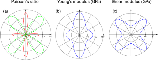
Figure 10: The orientation-dependent in-plane (a) of Poisson’s ratio, (b) Young’s modulus, and (c) shear modulus of $\delta$-phosphorene.

Test case (4): $\bm{\delta}$-Phosphorene. Haidi Wang et al. Wang et al. (2017) have discovered that $\delta$-phosphorene is a superior 2D auxetic material with high NPR. In Fig. 10, the Poisson’s ratio, shear modulus, and Young’s modulus are calculated by ElATools and shown by the dat2gnu.x and GNUPLOT. As shown in Fig. 10(a), the maximum value of the NPR (-0.267) occurs at a 90-degree angle. This amount is in perfect agreement with Haidi Wang et al. Also, the orientation-dependent Young’s modulus of this structure (see Fig. 10(b)) is in good agreement with Haidi Wang et al. ElATools can calculate shear modulus in 2D materials. Fig.10(c) shows this feature of $\delta$-phosphorene.

Test case (5): Pd₂O₆Se₂ monolayer. In this test case, the mechanical properties of the Pd₂O₆Se₂ monolayer with an oblique 2D crystal system are investigated. The values for the $C_{ij}$ was taken from computational 2D materials database (C2DB) Wang et al. (2017). In Fig. 11, the polar heat maps of Poisson’s ratio, Young’s modulus, and shear modulus are calculated by ElATools and shown by the dat2gnu.x and Gnuplot. The main elastic properties and anisotropy indices of this monolayer are listed in Table 12. It is clear from this table that the Pd₂O₆Se₂ monolayer has a NPR (-0.49). This result is well recognizable by polar heat maps (see Fig. 11). Polar heat maps in visualizing the mechanical properties of 2D materials, such as heat maps in 3D, are useful tools for searching for NPR with small values.

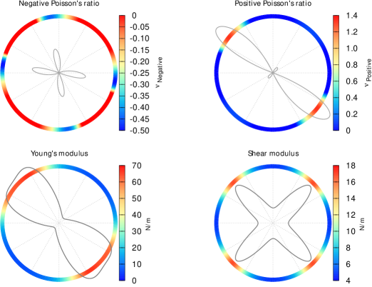
Figure 11: The polar heat maps of Poisson’s ratio, Young’s modulus, and shear modulus of Pd₂O₆Se₂ monolayer

Test case (6): NPR analysis of cubic symmetry materials. Arbitrarily large positive and negative values of Poisson’s ratio could occur in solids with cubic material symmetry Norris (2006); Baughman et al. (1998b). To investigate this matter, we have calculated the Poisson’s ratio of a hypothetical set of systems with cubic symmetry that include three independent elastic coefficients (C₁₁, C₁₂, and C₄₄) in the range between 0 and 100 GPa (with steps of 0.5 GPa), considering the mechanical stability criteria, and using ElATools.

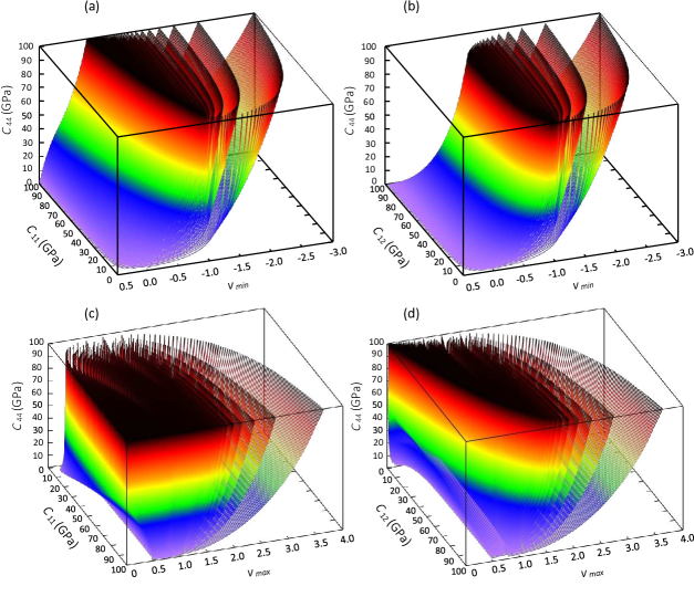
Figure 12: The minimum and maximum values of Poisson’s ratio diagram with respect to (a, b) (C₄₄, C₁₂) and (c, d) (C₄₄, C₁₁).

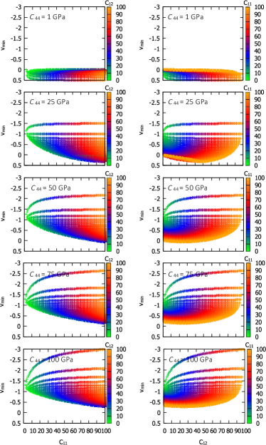
Figure 13: Five slices at constant values of C₄₄ in which the v_min is a function of C₁₁ and C₁₂ coefficients.

Fig. 12 shows the minimum (v_min) and maximum (v_max) values of Poisson’s ratio diagram with respect to (C₄₄, C₁₂) and (C₄₄, C₁₁). As shown in Figs. 12(a) and (b), C₄₄ plays a vital role in the negative values of v_min. Also, comparing these two figures, with increasing C₄₄, the value of C₁₁ has a more prominent role than the value of C₁₂ in NPR. For a better investigation, by combining Figs. 12(a-b) and Figs. 12(c-d), 5 slices in constant C₄₄ are shown in Fig. 13 and Fig. 14. In Fig. 13, v_min values are almost positive when C₄₄ =1 GPa and C₁₁ and C₁₂ range from 1 to 100 GPa. Few materials have been found that have such independent elastic coefficients. When C₄₄ increases from 1 to 50 GPa, for all C₁₁ and C₁₂, v_min changes its sign from positive to negative. As can be seen, when C₄₄ reaches 100 GPa, the maximum negative value of v_min is -3. In Fig. 14, when C₄₄ = 1 the maximum value of v_max is less than one, and with increasing C₄₄, the v_max increases and can reach 4. As shown in both Figs. 13 and 14, the patterns of changes in v_min and v_max are the same when v_min $\mathrm{<}$ -1 and v_max$\mathrm{>}$ 1. In general, it can be concluded that the coefficient of C₄₄ has a more critical role than the other two coefficients (C₁₁ and C₁₂) in the NPR of materials. These negative values of v_min also appear when stretched along the [110] direction.There are many compounds of cubic symmetry that can be placed in this range of elastic coefficients that can have NPR.

Finally, we have prepared a documentation website that provides more examples and tutorials for ElATools.

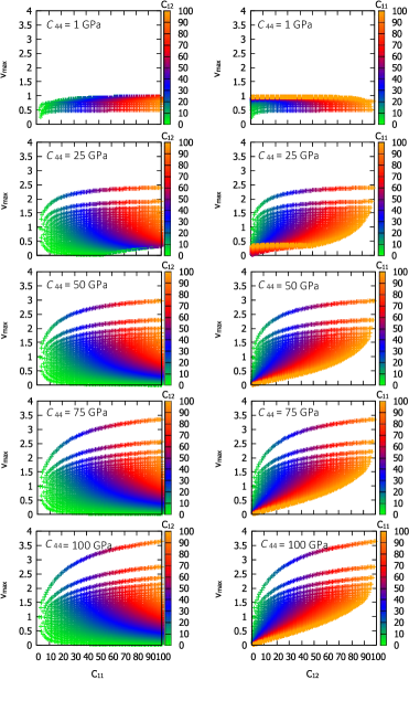
Figure 14: Five slices at constant values of C₄₄ in which the v_max is a function of C₁₁ and C₁₂ coefficients.

IV Summary and outlook

We introduced ElATools, a Fortran90 code designed to analyze the second-order elastic tensors of three and two-dimensional crystal systems. ElATools offers a helpful tool for detecting elastic anisotropy, NLC, and NPR or auxetic materials. Four post-processing programs specifically designed for the visualization of the results are provided. Besides, ElATools includes the elastic constant database of Materials Project for 3D materials allowing offline/online use. Furthermore, the code can generate data for Machine Learning to detect and predict elastic and anisotropy properties. The authors plan to extend ElATools to analyze other tensorial properties, such as piezoelectric and photoelastic tensors.

IV.1 Appendix A

A list of main elastic properties and anisotropy indices of two-dimensional and three-dimensional materials is provided in Table 2. The elastic modulus B, E, and G are defined by Eqs.(35), (36), and (37). Isotropic Poisson’s ratio and 2D Poisson’s ratio in 3D and 2D materials are defined by Eqs.(37) and (42), respectively.

The P-wave modulus (M), known as the longitudinal modulus, is associated with the homogeneous isotropic linear elastic materials. This modulus describes the ratio of axial stress to the axial strain in a uniaxial strain state Mavko et al. (2020), and is defined as follows:

$$M=B+4G/3.$$ (43)

Pugh’s ratio or B/G ratio defines the ductility or brittleness of a given material. The critical value of Pugh’s ratio is found to be 1.75. Materials with B/G $>$ 1.75 are ductile, whereas those with B/G $<$ 1.75 are brittle in nature Yalameha and Vaez (2018); Saeidi et al. (2019b); Pavlic et al. (2017).

Lame’s first ($\lambda_{1}$) and second ($\lambda_{2}$) parameters help to parameterize Hooke’s law in 3D for homogeneous and isotropic materials using the stress and strain tensors. The $\lambda_{1}$ provides a measure of compressibility, and the $\lambda_{2}$ is associated with the shear stiffness of a given material Mavko et al. (2020). These two parameters are specified as follows:

$$\lambda_{1}=\dfrac{\nu E}{(1+\nu)(1-2\nu)},\,\,\lambda_{2}=\dfrac{E}{2(1+\nu)}.$$ (44)

Kleinman’s parameter ($\xi$) describes the stability of a solid under stretching or bending, and is defined as follows:

$$\xi=\dfrac{C_{11}+8C_{12}}{7C_{11}-2C_{12}}.$$ (45)

$\xi$ = 1 implies that bond stretching would be dominated, while $\xi$ = 0 implies that bond bending would be dominated.

Thermal conductivity, responsible for conducting heat energy, is a useful physical parameter for practical applications. It decreases with increasing temperature toward a limiting value known as the minimum thermal conductivity ($\kappa_{m}$). The value of $\kappa_{m}$ can be obtained using Cahill Cahill et al. (1992) and Clarke Clarke and Levi (2003) models from the following expressions:

$$\kappa_{m}^{Clarke}=0.87k_{B}M_{a}^{2/3}E^{1/2}\rho^{1/6},$$ (46)

$$\kappa_{m}^{Cahill}=(k_{B}/2.48)n^{2/3}(\nu_{l}+2\nu_{t}),$$ (47)

where $k_{B}$ is Boltzmann’s constant, E and $\rho$ are Young’s modulus and the density of the material, respectively, and $M_{a}$ is the mean mass of atoms in each unit cell, which can be calculated by $M_{a}$=[M/(m$N_{A}$ )] (M and m are the molar mass and the total number of atoms in each unit cell, respectively, and $N_{A}$ is Avogadro’s constant). In Cahill’s model, n is the density of the atom number per unit volume, and $\nu_{l}$ and $\nu_{t}$ are the longitudinal and transverse sound velocities, respectively (see Eqs. (63),(64) and (65)). Currently, ElaTools calculates the $\kappa_{m}$ value by Clarke’s model.

Cauchy’s pressure ($P_{C}$) is associated with the angular characteristic of atomic bonding in a given material and is defined in different symmetries by Eqs. (39), (40), and (41).

Elastic anisotropy is an important property to characterize for a comprehensive understanding of the mechanical and physical properties of materials. This property influences a variety of physical processes like geophysical explorations of the Earth’s interior Berryman (1979), development of plastic deformation in crystals Li et al. (2002), enhanced positively charged defect mobility Brugués et al. (2008), microscale cracking in ceramics Tvergaard and Hutchinson (1988), alignment or misalignment of quantum dots Pei et al. (2003), etc. Various methods have been reported in the literature to quantify the elastic anisotropy based on elastic modulus and $C_{ij}$ tensor. Ranganathan and Ostoja-Starzewski Ranganathan and Ostoja-Starzewski (2008b) derived a universal anisotropy index $A^{U}$ to provide a measure of elastic anisotropy. This index is called universal because of its applicability to all crystal symmetries and can be defined as follows Ranganathan and Ostoja-Starzewski (2008b):

$$A^{U}=\dfrac{B_{V}}{B_{R}}+5\dfrac{G_{V}}{G_{R}}-6$$ (48)

According to the Ranganathan and Ostoja-Starzewski equation, Li et al.Li et al. (2020) suggested the following anisotropy index (A^R) for 2D materials:

$$A^{R}=\dfrac{B_{V}}{B_{R}}+2\dfrac{G_{V}}{G_{R}}-3$$ (49)

which B_V/B_R and G_V/G_R are area and shear modules in Voigt and Reuss approximations, respectively, which can be defined as follows Li et al. (2020):

$$B_{R}=\dfrac{1}{S_{11}+S_{22}+2S_{12}},B_{V}=\dfrac{C_{11}+C_{22}+2C_{12}}{4},$$ (50)

$$G_{R}=\dfrac{2}{S_{11}+S_{22}-2S_{12}+S_{66}},G_{V}=\dfrac{C_{11}+C_{22}-2C_{12}+4C_{66}}{8}.$$ (51)

Zener proposed an anisotropy factor ($A^{Z}$) for crystals of cubic symmetry defined as the ratio of the extreme values of the orientation-dependent shear moduli given by Zener (1948)

$$A^{Z}=\dfrac{2C_{44}}{C_{11}-C_{12}}$$ (52)

On the other hand, Chung and Buessem Berryman (1979) observed that a (Cubic) crystal is isotropic when the Voigt average of the shear moduli $G_{V}$ over all possible orientations was equal to the inverse of the orientation averaged shear compliance (Reuss average)$G_{R}$, which motivated the adoption of the factor

$$A^{BC}=\dfrac{G_{V}-G_{R}}{G_{V}+G_{R}}$$ (53)

$A^{BC}$= 0 for isotropic materials, and any positive deviation from this limiting value would indicate an anisotropic behavior. With this definition, one can determine whether a given cubic crystal is more anisotropic than the other. This index is defined as follows:

$$A^{L}=\sqrt{ln(\dfrac{B_{V}}{B_{R}})^{2}+5\,ln(\dfrac{G_{V}}{G_{R}})^{2}}$$ (54)

The Kube’s log-Euclidean anisotropy ($A^{L}$) is the most general definition of elastic anisotropy at present, as it was defined to make definitive comparisons between any two crystals. The isotropy is determined by $A^{L}$ = 0 and any positive value denotes a measure of the elastic anisotropy.

Two similar anisotropy indices A^K and A^SU with the above equation, have been proposed by Li et al. for 2D materials as follows Li et al. (2020):

$$A^{SU}=\sqrt{(\dfrac{{B_{V}}}{B_{R}}-1)^{2}+2(\dfrac{{G_{V}}}{G_{R}}-1)^{2}},$$ (55)

$$A^{K}=\sqrt{(ln\dfrac{{B_{V}}}{B_{R}})^{2}+2(ln\dfrac{{G_{V}}}{G_{R}})^{2}},$$ (56)

Since hardness is an essential property that is essential to describe the mechanical behavior fully various semi-empirical relations have been proposed to estimate hardness using the elastic moduli. In ElaTools package, the following semi-empirical correlations Ivanovskii (2013) between Vickers hardness ($H_{V}$) and B, G, E, $\nu$, and B/G, so-called macroscopic models for hardness prediction Tian et al. (2012); Jiang et al. (2011); Teter (1998); Jiang et al. (2010), are used:

$$H_{1a}=0.0963B,$$ (57)

$$H_{1b}=0.0607E,$$ (58)

$$H_{2}=-2.899+0.1769G,$$ (59)

$$H_{3}=0.0635E,$$ (60)

$$H_{4}=\dfrac{B(1-2\nu)}{6(1+\nu)},$$ (61)

$$H_{5}=2(\dfrac{G^{2}}{B})^{0.585}-3.$$ (62)

To determine the aptitude of the above methods in predicting hardness for different types of materials, we have used the model proposed by Singh et al. Singh et al. (2021). They found that the best model for these five hardness analysis methods correlates with the crystal class and the energy bandgap ($E_{g}$). Table 2 provides a selection guide for the best method for calculating hardness for different types of compounds.

The longitudinal ($\nu_{l}$), transverse ($\nu_{t}$), and average ($\nu_{m}$) elastic wave velocities can be calculated from the knowledge of the B and G, and $\rho$ as follows Anderson (1963):

$$\nu_{l}=\dfrac{3B+4G}{3\rho},$$ (63)

$$\nu_{t}=\sqrt{\dfrac{G}{\rho}},$$ (64)

$$\nu_{m}=[\dfrac{1}{3}(\dfrac{2}{\nu_{t}^{3}}+\dfrac{1}{\nu_{l}^{3}})]^{-1/3}.$$ (65)

where G and B denote $G_{VRH}$ and $B_{VRH}$, respectively. Moreover, these equations imply that one can obtain the elastic moduli and elastic constants by measuring the elastic wave velocities using ultrasonic waves.

Table 2: A guide to select the best hardness calculation method as a function of the crystal class and bandgap ($E_{g}$). This model was proposed by Singh et al. Singh et al. (2021)

Type of material	Cubic	Hexagonal	Orthorhombic	Rhombohedral	General
Insulator ($E_{g}$ > 2 eV)	$H_{2}$	$H_{1b}$	$H_{2}$	$H_{2}$	$H_{2}$
Semiconductor (0< $E_{g}$ < 2 eV)	$H_{5}$	$H_{1b}$, $H_{3}$	-	$H_{2}$	$H_{5}$
Metal ($E_{g}$ = 0)	$H_{1a}$	$H_{4}$	$H_{4}$	$H_{4}$	$H_{4}$

Table 3: List of the main elastic (wave) properties and anisotropy indices of 2D and 3D materials.

Properties		Formulae(s)
Elastic moduli and elastic parameters	Bulk modulus (B)	Eqs.(35) and (36)
	Young’s modulus (E)	Eq.(37)
	Shear modulus (G)	Eqs.(35) and (36)
	P-wave modulus (M)	Eq.(43)
	Poisson’s ratio ($\nu$)	Eqs.(37) and (42)
	Pugh’s ratio (B/G)	B/G
	Lame’s first parameter ($\lambda_{1}$)	Eq.(44)
	Lame’s second parameter ($\lambda_{2}$)	Eq.(44)
	Kleinman’s parameter ($\xi$)	Eq.(45)
	Minimum thermal conductivity ($\kappa_{m}$)	Eq.(46)
Cauchy’s pressures (PC)	Cubic symmetry	Eq.(39)
	Hex., Trig., and Tetra. symmetries	Eq.(40)
	Orthorhombic symmetry	Eq.(41)
Elastic anisotropy indices	Universal anisotropy index (AU)	Eq.(48)
	Zener’s anisotropy index (AZ)	Eq.(52)
	Ranganathan anisotropy index (AR)	Eq.(49)
	Chung-Buessem anisotropy index (ACB)	Eq.(53)
	Kube’s log-Euclidean anisotropy index (AL)	Eq.(54)
	2D anisotropy index (ASU)	Eq.(55)
	Kube anisotropy index (AK)	Eq.(56)
Hardness methods	H1a	Eq.(57)
	H1b	Eq.(58)
	H2	Eq.(59)
	H3	Eq.(60)
	H4	Eq.(61)
	H5	Eq.(62)
Elastic wave properties	Longitudinal elastic wave velocity ($v_{l}$)	Eq.(63)
	Transverse elastic wave velocity ($v_{t}$)	Eq.(64)
	Main elastic wave velocity ($v_{m}$)	Eq.(65)

IV.2 Appendix B

List of input, output, and temporary files in Table 3. The three executables dat2gnu.x, dat2html.x, and dat2wrl.x are called with input command “pro” (for 3D representations and 2D projections) and “hmpro” (for 2D head maps). The executable dat2agr.x runs two input commands, box (boxpro), and polar (polarpro) used for 2D projections in cartesian and polar coordinates, respectively. The full details of the input commands and the displayable features of each of these post-processing codes are listed in Tables 5, 6, and 7.

Table 4: List of input, output, and temporary files related to Elatools.x, dat2gnu.x, dat2agr.x, dat2wrl.x, and dat2html.x executables.

Program	Input comment	Input file(s)	Output file(s	Temporary file(s)
ElATools	-	Cij.dat, Cij-2D.dat, INVELC-matrix, elast.output, ELADAT, ElaStic_2nd.out	Sij.dat, DATA.dat, 2dcut_pro.dat 1 , 3d_pro.dat, pro_2d_sys.dat	HKL, MESH, .aelastpro, .MaMiout, 3d_SD.dat
dat2gnu	pro, hmpro, phmpro 2	2dcut_pro.dat, HKL, .MaMiout, 3d_SD.dat	gpi files	.SDdat
dat2agr	polar, box, boxpro, polarpro	2dcut_pro.dat	agr files	-
dat2wrl	pro	3d_pro.dat, .aelastpro, .MaMiout	wrl files	-
dat2html	pro	3d_pro.dat MESH	html files	-

• pro: bulk, comp, poisson, young, shear, pp, pf, ps, gp, gf, gs, pfp, pff, pfs, km, etc.

• The full list of input comments is in Table 5, 6, and 7. Note that the current features and options of the ElaTools package may increase in future versions.

Table 5: List of input commands, and input files related to dat2gnu.x executable.

Input comment	Input file	Property	Type of graph
poi	2dcut_poisson.dat	$\nu$	Polar coordinates for 3D system
young	2dcut_young.dat	E
bulk	2dcut_bulk.dat	B
shear	2dcut_shear.dat	G
comp	2dcut_comp.dat	$\beta$
pp	2dcut_pveloc.dat	$\nu_{p}$: P-mode
ps	2dcut_pveloc.dat	$\nu_{p}$: Show-mode
pf	2dcut_pveloc.dat	$\nu_{p}$: Fast-mode
gp	2dcut_gveloc.dat	$\nu_{g}$: P-mode
gs	2dcut_gveloc.dat	$\nu_{g}$: Show-mode
gf	2dcut_gveloc.dat	$\nu_{g}$: Fast-mode
pfp	2dcut_pfaveloc.dat	PFA: P-mode
pfs	2dcut_pfaveloc.dat	PFA: Show-mode
pff	2dcut_pfaveloc.dat	PFA: Fast-mode
pall	2dcut_pveloc.dat	$\nu_{p}$: All modes
gall	2dcut_gveloc.dat	$\nu_{g}$: All modes
pfall	2dcut_pfaveloc.dat	PFA: All modes
km	3d_km.dat	$\kappa_{m}$
hmpoi	3d_poisson.dat	$\nu$	Heat map diagram for 3D system
hmyoung	3d_young.dat	E
hmbulk	3d_bulk.dat	B
hmcomp	3d_comp.dat	$\beta$
hmshear	3d_bulk.dat	G
hmpall	3d_pp.dat, 3d_ps.dat, 3d_pf.dat	$\nu_{p}$: All modes
hmgall	3d_gp.dat, 3d_gs.dat, 3d_gf.dat	$\nu_{g}$: All modes
hmpfall	3d_pfp.dat, 3d_pfs.dat, 3d_pff.dat	PFA: Fast-mode
hmkm	3d_km.dat	$\kappa_{m}$
2dpoi	poisson_2d_sys.dat	$\nu$	Polar coordinates for 2D system
2dyoung	young_2d_sys.dat	E
2dshear	shear_2d_sys.dat	G
phmpoi	poisson_2d_sys.dat	$\nu$	Polar heat map diagram for 2D system
phmyou	young_2d_sys.dat	E
phmshe	shear_2d_sys.dat	G

Table 6: List of input commands, and input files related to dat2wrl.x and dat2html.x executables.

Input comment	Input file(s)	Property	Type of graph
poi	3d_poisson.dat	$\nu$	Spherical coordinates for 3D system
young	3d_young.dat	E
bulk	3d_bulk.dat	B
shear	3d_shear.dat	G
comp	3d_comp.dat	$\beta$
pp	3d_pp.dat	$\nu_{p}$: P-mode
ps	3d_ps.dat	$\nu_{p}$: Show-mode
pf	3d_pf.dat	$\nu_{p}$: Fast-mode
gp	3d_gp.dat	$\nu_{g}$: P-mode
gs	3d_gs.dat	$\nu_{g}$: Show-mode
gf	3d_gf.dat	$\nu_{g}$: Fast-mode
pfp	3d_pfp.dat	PFA: P-mode
pfs	3d_pfs.dat	PFA: Show-mode
pff	3d_pff.dat	PFA: Fast-mode
pall	3d_pp.dat, 3d_ps.dat, 3d_pf.dat	$\nu_{p}$: All modes
gall	3d_gp.dat, 3d_gs.dat, 3d_gf.dat	$\nu_{g}$: All modes
km	3d_km.dat	$\kappa_{m}$

Table 7: List of input commands, and input files related to dat2agr.x executable.

Input comment	Input file(s)	Property	Type of graph
box	2dcut_young.dat, 2dcut_shear.dat, 2dcut_buk.dat, 2dcut_comp.dat, 2dcut_poisson.dat	E, G, B, $\beta$, and $\nu$: multiplot	Polar coordinates of 2D cuts in the 3D system
boxpoi	2dcut_poisson.dat	$\nu$
boxyoung	2dcut_young.dat	E
boxbulk	2dcut_buk.dat	B
boxshear	2dcut_shear.dat	G
boxcomp	2dcut_comp.dat	$\beta$
boxkm	2dcut_km.dat	$\kappa_{m}$
boxpall	2dcut pveloc.dat	$\nu_{p}$: All modes
boxgall	2dcut gveloc.dat	$\nu_{g}$: All modes
boxpfall	2dcut pdveloc.dat	PFA: All modes
polar	2dcut_young.dat, 2dcut_shear.dat, 2dcut_buk.dat, 2dcut_comp.dat, 2dcut_poisson.dat	E, G, B, $\beta$, and $\nu$: multiplot	Cartesian coordinates of 2D cuts in the 3D system
polarpoi	2dcut_poisson.dat	$\nu$
polaryoung	2dcut_young.dat	E
polarbulk	2dcut_buk.dat	B
polarshear	2dcut_shear.dat	G
polarcomp	2dcut_comp.dat	$\beta$
polarkm	2dcut_km.dat	$\kappa_{m}$
polarpall	2dcut_pveloc.dat	$\nu_{p}$: All modes
polargall	2dcut_gveloc.dat	$\nu_{g}$: All modes
polarpfall	2dcut_pfveloc.dat	PFA: All modes

IV.3 Appendix C

List of main elastic properties and anisotropy indices of ZnAu₂(CN)₄, GaAs, CrB₂, $\delta$-phosphorene ($\delta$-P), and Pd₂O₆Se₂ compounds. The ElATools also calculates a measure of the anisotropy A_M of each elastic modulus M, defined as follows:

$$A_{M}=\begin{cases}\frac{M_{MAX}}{M_{MIN}}&;if\ sign(M_{MAX})=sign(M_{MAX})\\ \infty&\ ;otherwise\end{cases}$$ (66)

$A_{M}$ is particularly interesting as the marked anisotropy of the mechanical properties is often associated with anomalous mechanical behavior, such as NPR and NLC. As can be seen in Table IV, when $A_{M}$ is infinite, the material has anomalous mechanical properties.

Table 8: The main elastic properties of ZnAu₂(CN)₄ compound.

Elastic properties	Bulk modulus (GPa)	Shear modulus (GPa)	Young modulus (GPa)	Poisson’s ratio	Pugh ratio	P-wave modulus (GPa)	Linear Compressibility (TPa-1)
Max	5.747×102	12.10	28.25	1.255	-	-	62.328
Min	-5.477×102	3.18	7.26	-0.021	-	-	-51.689
Voigt	55.756	8.753	24.954	0.4254	6.3696	67.4267	-
Reuss	13.705	4.618	12.456	0.4597	2.9674	19.8627	-
Average (Hall)	34.730	6.686	18.705	0.4426	5.1945	43.6447	-
$\textbf{A}_{\textbf{M}}$	$\infty$	3.804	3.893	$\infty$	-	-	$\infty$

Table 9: The main elastic properties of the CrB₂ compound.

Elastic properties	Bulk modulus (GPa)	Shear modulus (GPa)	Young modulus (GPa)	Poisson’s ratio	Pugh ratio	P-wave modulus (GPa)	Linear Compressibility (TPa-1)
Max	11.922×102	197.40	463.18	0.453	-	-	1.869
Min	5.351×102	125.04	260.22	0.162	-	-	0.839
Voigt	295.122	169.833	427.497	0.2586	1.7377	521.5667	-
Reuss	282.009	161.560	406.966	0.2595	1.7455	497.4226	-
Average (Hall)	288.565	165.697	417.231	0.2635	1.7415	509.4947	-
$\textbf{A}_{\textbf{M}}$	2.227	1.579	1.780	2.793	-	-	2.228

Table 10: List of Maximum (Max), minimum (Min) phase and group velocities, and anisotropy values of GaAs compound.

Property	Phase velocity (km/s)			Group velocity (km/s)
	P mode	FS mode	SS mode	P mode	FS mode	SS mode
Max	5.398	3.346	3.346	5.398	3.369	3.490
Min	4.731	2.805	2.475	4.731	2.935	2.476
AM	1.14	1.19	1.35	1.14	1.15	1.41

Table 11: The main elastic properties of the $\delta$-P 2D compound.

Elastic properties	Area modulus (N/m)	Shear modulus (N/m)	Young modulus (N/m)	Poisson’s ratio
Max	-	66.452	142.877	0.290
Min	-	24.500	62.277	-0.267
Voigt	47.608	47.909	-	-
Reuss	44.395	35.808	-	-
xy-plane	-	24.500	-	-0.159
yx-plane	-	-	-	-0.267
x-direction	-	-	84.872	-
y-direction	-	-	142.868	-

Table 12: The main elastic properties of the Pd₂O₆Se₂ 2D compound.

Elastic properties	Area modulus (N/m)	Shear modulus (N/m)	Young modulus (N/m)	Poisson’s ratio
Max	-	16.682	65.892	1.315
Min	-	4.857	6.573	-0.492
Voigt	23.445	15.828	-	-
Reuss	7.686	7.524	-	-
xy-plane	-	14.930	-	0.168
yx-plane	-	-	-	0.164
x-direction	-	-	39.731	-
y-direction	-	-	38.390	-

Table 13: List of anisotropy indices of ZnAu₂(CN)₄, CrB₂, $\delta$-phosphorene ($\delta$-P), and Pd₂O₆Se₂ compounds.

Anisotropy index
and Cauchy pressure	Compounds
	ZnAu2(CN)4	CrB2	$\delta$-P	Pd2O6Se2
AU	7.5448	0.3025	-	-
AL	4.7370	0.3025	-	-
ACB	0.3092	0.0250	-	-
ASU	-	-	0.4833	2.5760
AR	-	-	0.7482	4.2574
AK	-	-	0.1814	0.6657
P${}_{C}^{a}$	48.50	25.90		-
P${}_{C}^{c}$	26.50	-15.60		-

IV.4 Appendix D

Colors available in the visualization of elastic properties in the ElATools. Personalization of colors is provided in the Supplementary Information file.

Table 14: List of default colors in the 3D and 2D visualization of elastic properties such as Young’s modulus, bulk modulus, shear modulus, linear compressibility, and Poisson’s ratio.

3D or 2D representation of elastic proprieties	Positive value or Maximum positive value	Minimum positive value	Negative value or Minimum Negative value
Young’s modulus	green	-	-
Bulk modulus	green	-	-
Shear modulus	bule	green	-
Linear compressibility	green	-	red
Poisson’s ratio	blue	green	red

V acknowledgement

Parviz Saeidi is acknowledged for the valuable comments on the first draft of the manuscript.

VI References

References

- Ledbetter and Reed (1973) H. M. Ledbetter and R. P. Reed, Journal of Physical and Chemical Reference Data 2, 531 (1973).
- Li and Bradt (1987) Z. Li and R. C. Bradt, Journal of materials science 22, 2557 (1987).
- Turner et al. (1990) C. H. Turner, S. C. Cowin, J. Y. Rho, R. B. Ashman, and J. C. Rice, Journal of biomechanics 23, 549 (1990).
- Yoon and Newnham (1969) H. S. Yoon and R. Newnham, American Mineralogist: Journal of Earth and Planetary Materials 54, 1193 (1969), https://pubs.geoscienceworld.org/msa/ammin/article-pdf/54/7-8/1193/4249496/am-1969-1193.pdf .
- Saeidi et al. (2019a) P. Saeidi, S. Yalameha, and Z. Nourbakhsh, Physics Letters A 383, 221 (2019a).
- Yalameha and Vaez (2018) S. Yalameha and A. Vaez, International Journal of Modern Physics B 32, 1850129 (2018).
- Yalameha et al. (2020) S. Yalameha, P. Saeidi, Z. Nourbakhsh, A. Vaez, and A. Ramazani, Journal of Applied Physics 127, 085102 (2020).
- Tehrani and Brgoch (2019) A. M. Tehrani and J. Brgoch, Journal of Solid State Chemistry 271, 47 (2019).
- Lay and Wallace (1995) T. Lay and T. C. Wallace, Modern global seismology (Elsevier, 1995).
- Tatsumi et al. (2003) K. Tatsumi, I. Tanaka, K. Tanaka, H. Inui, M. Yamaguchi, H. Adachi, and M. Mizuno, Journal of Physics: Condensed Matter 15, 6549 (2003).
- McSkimin (1950) H. McSkimin, The Journal of the Acoustical Society of America 22, 413 (1950).
- Vacher and Boyer (1972) R. Vacher and L. Boyer, Phys. Rev. B 6, 639 (1972).
- Parr and Yang (1995) R. G. Parr and W. Yang, Annual Review of Physical Chemistry 46, 701 (1995), pMID: 24341393, https://doi.org/10.1146/annurev.pc.46.100195.003413 .
- Hohenberg and Kohn (1964) P. Hohenberg and W. Kohn, Phys. Rev. 136, B864 (1964).
- Kohn and Sham (1965) W. Kohn and L. J. Sham, Phys. Rev. 140, A1133 (1965).
- Sun et al. (2003) G. Sun, J. Kürti, P. Rajczy, M. Kertesz, J. Hafner, and G. Kresse, Journal of Molecular Structure: THEOCHEM 624, 37 (2003).
- Dovesi et al. (2014) R. Dovesi, R. Orlando, A. Erba, C. M. Zicovich-Wilson, B. Civalleri, S. Casassa, L. Maschio, M. Ferrabone, M. De La Pierre, P. D’Arco, Y. Noël, M. Causà, M. Rérat, and B. Kirtman, International Journal of Quantum Chemistry 114, 1287 (2014), https://onlinelibrary.wiley.com/doi/pdf/10.1002/qua.24658 .
- Blaha et al. (2020) P. Blaha, K. Schwarz, F. Tran, R. Laskowski, G. K. H. Madsen, and L. D. Marks, The Journal of Chemical Physics 152, 074101 (2020), https://doi.org/10.1063/1.5143061 .
- Jamal et al. (2018) M. Jamal, M. Bilal, I. Ahmad, and S. Jalali-Asadabadi, Journal of Alloys and Compounds 735, 569 (2018).
- Golesorkhtabar et al. (2013) R. Golesorkhtabar, P. Pavone, J. Spitaler, P. Puschnig, and C. Draxl, Computer Physics Communications 184, 1861 (2013).
- Giannozzi et al. (2009) P. Giannozzi, S. Baroni, N. Bonini, M. Calandra, R. Car, C. Cavazzoni, D. Ceresoli, G. L. Chiarotti, M. Cococcioni, I. Dabo, et al., Journal of physics: Condensed matter 21, 395502 (2009).
- Gulans et al. (2014) A. Gulans, S. Kontur, C. Meisenbichler, D. Nabok, P. Pavone, S. Rigamonti, S. Sagmeister, U. Werner, and C. Draxl, Journal of Physics: Condensed Matter 26, 363202 (2014).
- Jain et al. (2013) A. Jain, S. P. Ong, G. Hautier, W. Chen, W. D. Richards, S. Dacek, S. Cholia, D. Gunter, D. Skinner, G. Ceder, and K. A. Persson, APL Materials 1, 011002 (2013), https://doi.org/10.1063/1.4812323 .
- Cairns and Goodwin (2015) A. B. Cairns and A. L. Goodwin, Physical Chemistry Chemical Physics 17, 20449 (2015).
- Evans (1991) K. E. Evans, Endeavour 15, 170 (1991).
- Saeidi et al. (2019b) P. Saeidi, S. Yalameha, et al., Computational Condensed Matter 18, e00358 (2019b).
- Ortiz et al. (2012) A. U. Ortiz, A. Boutin, A. H. Fuchs, and F.-X. Coudert, Physical review letters 109, 195502 (2012).
- Marmier et al. (2010) A. Marmier, Z. A. Lethbridge, R. I. Walton, C. W. Smith, S. C. Parker, and K. E. Evans, Computer Physics Communications 181, 2102 (2010).
- Lakes (1987) R. Lakes, Science 235, 1038 (1987).
- Baughman et al. (1998a) R. H. Baughman, S. Stafström, C. Cui, and S. O. Dantas, Science 279, 1522 (1998a).
- Miller et al. (2015) W. Miller, K. E. Evans, and A. Marmier, Applied Physics Letters 106, 231903 (2015).
- Bridgman (1922) P. W. Bridgman, Proceedings of the National Academy of Sciences of the United States of America 8, 361 (1922).
- Fortes et al. (2011) A. D. Fortes, E. Suard, and K. S. Knight, Science 331, 742 (2011).
- Gaillac et al. (2016) R. Gaillac, P. Pullumbi, and F.-X. Coudert, Journal of Physics: Condensed Matter 28, 275201 (2016).
- Singh et al. (2021) S. Singh, L. Lang, V. Dovale-Farelo, U. Herath, P. Tavadze, F.-X. Coudert, and A. H. Romero, Computer Physics Communications 267, 108068 (2021).
- Hunter (2007) J. D. Hunter, Computing in Science and Engineering 9, 90 (2007).
- C.B. Sullivan (2019) A. K. C.B. Sullivan, Journal of Open Source Software 4, 1450 (2019).
- Ranganathan and Ostoja-Starzewski (2008a) S. I. Ranganathan and M. Ostoja-Starzewski, Physical Review Letters 101, 055504 (2008a).
- Kube (2016) C. M. Kube, AIP Advances 6, 095209 (2016).
- Kleinman (1962) L. Kleinman, Phys. Rev. 128, 2614 (1962).
- Hill (1952) R. Hill, Proceedings of the Physical Society. Section A 65, 349 (1952).
- Kamburelis and other Castle Game Engine developers (2020) M. Kamburelis and other Castle Game Engine developers, View3dscene (2020).
- Team (2008) G. D. Team, Grace (2008).
- Janert (2010) P. K. Janert, Gnuplot in action: understanding data with graphs (Manning, 2010).
- Nye et al. (1985) J. F. Nye et al., Physical properties of crystals: their representation by tensors and matrices (Oxford university press, 1985).
- Nordmann et al. (2018) J. Nordmann, M. Aßmus, and H. Altenbach, Continuum Mechanics and Thermodynamics 30, 689 (2018).
- Zhao et al. (2016) T. Zhao, S. Zhang, Y. Guo, and Q. Wang, Nanoscale 8, 233 (2016).
- Jasiukiewicz et al. (2008) C. Jasiukiewicz, T. Paszkiewicz, and S. Wolski, physica status solidi (b) 245, 562 (2008).
- Jasiukiewicz et al. (2010) C. Jasiukiewicz, T. Paszkiewicz, and S. Wolski, physica status solidi (b) 247, 1247 (2010).
- Auld and Fields (1990) B. Auld and A. Fields, Malabar, Florida (1990).
- Koos and Wolfe (1984) G. Koos and J. Wolfe, Physical Review B 29, 6015 (1984).
- Voigt et al. (1928) W. Voigt et al., Lehrbuch der kristallphysik, Vol. 962 (Teubner Leipzig, 1928).
- Reuss (1929) A. Reuss, Z. Angew. Math. Mech 9, 49 (1929).
- Pugh (1954) S. Pugh, The London, Edinburgh, and Dublin Philosophical Magazine and Journal of Science 45, 823 (1954).
- Pettifor (1992) D. Pettifor, Materials science and technology 8, 345 (1992).
- Qu et al. (2020) D. Qu, C. Li, L. Bao, Z. Kong, and Y. Duan, Journal of Physics and Chemistry of Solids 138, 109253 (2020).
- Duan et al. (2021) Y. Duan, Y. Wang, M. Peng, and K. Wang, Materials Today Communications 26, 101991 (2021).
- Boochani et al. (2019) A. Boochani, M. Jamal, M. Shahrokhi, B. Nowrozi, M. B. Gholivand, J. Khodadadi, E. Sartipi, M. Amiri, M. Asshabi, and A. Yari, Journal of Materials Chemistry C 7, 13559 (2019).
- Zhang and Zhang (2017) S. Zhang and R. Zhang, Computer Physics Communications 220, 403 (2017).
- Sievert (2020) C. Sievert, Interactive Web-Based Data Visualization with R, plotly, and shiny (Chapman and Hall/CRC, 2020).
- Gupta et al. (2017) M. K. Gupta, B. Singh, R. Mittal, M. Zbiri, A. B. Cairns, A. L. Goodwin, H. Schober, and S. L. Chaplot, Physical Review B 96, 214303 (2017).
- Chong et al. (2014) X. Chong, Y. Jiang, R. Zhou, and J. Feng, Journal of alloys and compounds 610, 684 (2014).
- Auld (1973) B. A. Auld, Acoustic fields and waves in solids (Krieger Publishing Company, 1973).
- Haastrup et al. (2018) S. Haastrup, M. Strange, M. Pandey, T. Deilmann, P. S. Schmidt, N. F. Hinsche, M. N. Gjerding, D. Torelli, P. M. Larsen, A. C. Riis-Jensen, et al., 2D Materials 5, 042002 (2018).
- Wang et al. (2017) H. Wang, X. Li, P. Li, and J. Yang, Nanoscale 9, 850 (2017).
- Norris (2006) A. N. Norris, Proceedings of the Royal Society A: Mathematical, Physical and Engineering Sciences 462, 3385 (2006).
- Baughman et al. (1998b) R. H. Baughman, J. M. Shacklette, A. A. Zakhidov, and S. Stafström, Nature 392, 362 (1998b).
- Mavko et al. (2020) G. Mavko, T. Mukerji, and J. Dvorkin, The rock physics handbook (Cambridge university press, 2020).
- Pavlic et al. (2017) O. Pavlic, W. Ibarra-Hernandez, I. Valencia-Jaime, S. Singh, G. Avendano-Franco, D. Raabe, and A. H. Romero, Journal of Alloys and Compounds 691, 15 (2017).
- Cahill et al. (1992) D. G. Cahill, S. K. Watson, and R. O. Pohl, Physical Review B 46, 6131 (1992).
- Clarke and Levi (2003) D. Clarke and C. Levi, Annual review of materials research 33, 383 (2003).
- Berryman (1979) J. G. Berryman, Geophysics 44, 896 (1979).
- Li et al. (2002) J. Li, K. J. Van Vliet, T. Zhu, S. Yip, and S. Suresh, Nature 418, 307 (2002).
- Brugués et al. (2008) J. Brugués, J. Ignés-Mullol, J. Casademunt, and F. Sagués, Physical review letters 100, 037801 (2008).
- Tvergaard and Hutchinson (1988) V. Tvergaard and J. W. Hutchinson, Journal of the American Ceramic Society 71, 157 (1988).
- Pei et al. (2003) Q. Pei, C. Lu, and Y. Y. Wang, Journal of applied physics 93, 1487 (2003).
- Ranganathan and Ostoja-Starzewski (2008b) S. I. Ranganathan and M. Ostoja-Starzewski, Physical review letters 101, 055504 (2008b).
- Li et al. (2020) R. Li, Q. Shao, E. Gao, and Z. Liu, Extreme Mechanics Letters 34, 100615 (2020).
- Zener (1948) C. Zener, Elasticity and anelasticity of metals (University of Chicago press, 1948).
- Ivanovskii (2013) A. Ivanovskii, International Journal of Refractory Metals and Hard Materials 36, 179 (2013), special Section: Recent Advances of Functionally Graded Hard Materials.
- Tian et al. (2012) Y. Tian, B. Xu, and Z. Zhao, International Journal of Refractory Metals and Hard Materials 33, 93 (2012).
- Jiang et al. (2011) X. Jiang, J. Zhao, and X. Jiang, Computational Materials Science 50, 2287 (2011).
- Teter (1998) D. M. Teter, MRS bulletin 23, 22 (1998).
- Jiang et al. (2010) X. Jiang, J. Zhao, A. Wu, Y. Bai, and X. Jiang, Journal of Physics: Condensed Matter 22, 315503 (2010).
- Anderson (1963) O. L. Anderson, Journal of Physics and Chemistry of Solids 24, 909 (1963).