Abstract

With the aid of the relaxed polygonal inequality (introduced by Fagin et al.) we strive to extend the applicability of Christofides approximation technique to the scope of all complete finite weighted graphs with positive weights. First section acquaints the Reader with the class of semimetric graphs and proves that every finite graph admits $\gamma$-polygon structure. Sections 2 and 3 establish the necessary notions from the graph and optimization theory to tackle the Traveling Salesperson Problem. In section 4 the minimal spanning tree method is introduced, while section 5 focuses on the analysis of this method through the lens of $\gamma$-polygon graphs. The final section of the paper adjusts the technique of Christofides by obtaining $\frac{3\gamma}{2}-$approximation for the TSP.

Keywords : $b$-metric spaces, semimetric spaces, MST, TSP AMS: 54E25, 90C27, 68R10, 05C45,

1 Semimetric initial framework

In the past several decades we have witnessed the formation of close ties between discrete mathematics and the theory of metric spaces. The underlying reason for this “mathematical marriage” is that metric spaces constitute an abstract (but still useful) setting for various problems in discrete mathematics (this fact has already been emphasized by Piotr Indyk and Nathan Linial). As the years went by mathematicians started to fiddle with the generalizations of metric spaces and their possible applications to the realm of discrete mathematics. Among the most fruitful generalizations one should list hemimetric spaces (also known in the literature as quasimetric spaces), where the symmetry axiom “$d(x,y)=d(y,x)$” in the definition of metric is skipped. Such spaces emerge naturally when we measure time needed to traverse from point $A$ to point $B$ in the mountains (you need not be a highlander to know that the climb is usually longer than the descent). Another very popular generalization of the metric space is the pseudometric space, where the first axiom of a metric, i.e.

$$d(x,y)=0\ \iff x=y,$$

need not hold. It turns out that pseudometric spaces are especially common in the domain of fuzzy sets.

The applications of hemimetric and pseudometric spaces in various branches of mathematics are rather encouraging to say the least. Following that clue, our paper focuses on another family of spaces, called the semimetric spaces:

Definition 1.

For a nonempty set $X$, a function $d:X\times X\longrightarrow[0,+\infty)$ is called a semimetric if it satisfies the following two conditions:

• $\forall_{x,y\in X}\ d(x,y)=0\ \iff\ x=y$,

• $\forall_{x,y\in X}\ d(x,y)=d(y,x)$.

The pair $(X,d)$ is called a semimetric space.

Browsing through the literature one encounters multiple sources which assume that a semimetric space is first-countable. Throughout the paper we are only concerned with finite spaces (finite graphs to be precise), so the first-countability condition is satisfied, although not explicitely required in Definition 1.

Amongst all semimetric spaces it is convenient to distinguish those, which have some counterpart of the celebrated triangle inequality. For our purposes, let us introduce $\beta-$metric spaces and $\gamma-$polygon spaces:

Definition 2.

A semimetric space $(X,d)$ is said to be:

• $\beta-$metric space if $\beta\geqslant 1$ is the smallest number such that the semimetric $d$ satisfies the $\beta-$triangle inequality:

  $$\forall_{x,y,z\in X}\ d(x,z)\leqslant\beta(d(x,y)+d(y,z)),$$ (1)

• $\gamma-$polygon space if $\gamma\geqslant 1$ is the smallest number such that the semimetric $d$ satisfies the $\gamma-$polygon inequality:

  $$\forall_{n\in\mathbb{N}}\ \forall_{x_{1},\dots,x_{n}\in X}\ d(x_{1},x_{n})\leqslant\gamma\cdot\sum_{k=1}^{n-1}d(x_{k},x_{k+1}).$$ (2)

It goes without saying that every $\gamma-$polygon space is automatically a $\beta-$metric space with $\beta\leqslant\gamma$ (we will shortly provide an example that the constants need no coincide). Conversely, if we assume that $X$ is finite (as we do in this paper), then every $\beta-$metric space is a $\gamma-$polygon space with $\gamma\leqslant\beta^{|X|-1}.$ A closer inspection reveals that we have an estimate $\gamma\leqslant\beta^{\lceil\log_{2}(|X|-1)\rceil}$ (assuming that $X$ consists of more than one point).

It is a relatively easy, though still useful remark that every finite semimetric space admits both $\beta$-metric and $\gamma$-polygon structure:

Theorem 1.

Every finite semimetric space $(X,d)$ is a $\gamma-$polygon space with

$$\gamma=\sup\left\{\frac{d(x_{1},x_{n})}{\sum_{k=1}^{n-1}d(x_{k},x_{k+1})}\ :n\in\mathbb{N},\ x_{1},\dots,x_{n}\in X,\ x_{1}\neq x_{n}\right\}.$$ (3)

In particular, every finite semimetric space $(X,d)$ is a $\beta-$metric space with

$$\beta=\sup\left\{\frac{d(x,z)}{d(x,y)+d(y,z)}\ :\ x,y,z\in X,\ x\neq z\right\}.$$ (4)

Proof.

Without loss of generality, we can assume that the space $X$ contains at least $2$ elements (otherwise $(X,d)$ is trivially a $\gamma-$polygon space for any $\gamma\geqslant 1$). Let

$$s:=\sup\left\{\frac{d(x_{1},x_{n})}{\sum_{k=1}^{n-1}d(x_{k},x_{k+1})}\ :n\in\mathbb{N},\ x_{1},\dots,x_{n}\in X,\ x_{1}\neq x_{n}\right\}$$

and observe that it is a well-defined, finite number, which satisfies (for any choice of $x_{1},x_{2}\in X$ with $x_{1}\neq x_{2}$)

$$s\geqslant\frac{d(x_{1},x_{2})}{d(x_{1},x_{2})}=1.$$

Furthermore, let us fix $n\in\mathbb{N}$ and elements $x_{1},\dots,x_{n}\in X$ and consider two cases:

• if $x_{1}=x_{n}$ then

  $$d(x_{1},x_{n})=0\leqslant s\cdot\sum_{k=1}^{n-1}\ d(x_{k},x_{k+1});$$

• if $x_{1}\neq x_{n}$ then

  $$d(x_{1},d_{n}) = \frac{d(x_{1},x_{n})}{\sum_{k=1}^{n-1}\ d(x_{k},x_{k+1})}\cdot\sum_{k=1}^{n-1}\ d(x_{k},x_{k+1})$$

  $$\leqslant \sup\left\{\frac{d(y_{1},y_{n})}{\sum_{k=1}^{n-1}\ d(y_{k},y_{k+1})}\ :\ y_{1},\dots,y_{n}\in X,\ y_{1}\neq y_{n}\right\}\cdot\sum_{k=1}^{n-1}\ d(x_{k},x_{k+1})$$

  $$= s\cdot\sum_{k=1}^{n-1}\ d(x_{k},x_{k+1}).$$

This proves that $\gamma\leqslant s.$

In order to prove the reverse inequality suppose, for the sake of argument, that there exists $\varepsilon>0$ such that $\gamma=s-\varepsilon$. From the definition of supremum there exists an $n\in\mathbb{N}$ as well as some elements $x_{1},\dots,x_{n}\in X$ such that

$$\frac{d(x_{1},x_{n})}{\sum_{k=1}^{n-1}d(x_{k},x_{k+1})}>s-\varepsilon.$$

Multiplying both sides of this inequality yields

$$d(x_{1},x_{n})>(s-\varepsilon)\cdot\sum_{k=1}^{n-1}d(x_{k},x_{k+1}),$$

which contradicts the assumption that $\gamma<s$. This concludes the first part of the theorem (for $\gamma-$polygon space). In order to prove the second part (a finite semimetric space is a $\beta-$metric space) we follow an analogous reasoning as the one presented above, fixing $n=3$. ∎

At this point we know that given a finite semimetric space it has to be both $\beta-$metric and $\gamma-$polygon space at the same time. Moreover, we also know that $\beta\leqslant\gamma,$ but in general, these constants may differ. To illustrate that point let us discuss the following example:

Example 1.

Let $X:=\{1,2,3,4,5\}$ and let $d:X\times X\longrightarrow[0,+\infty)$ be a semimetric given by

$$d(x,y):=\begin{cases}0,&x=y,\\ 1,&|x-y|=1,\\ 20,&|x-y|=4,\\ 4,&\text{otherwise.}\end{cases}$$ (5)

See the following figure for the illustration of this space:

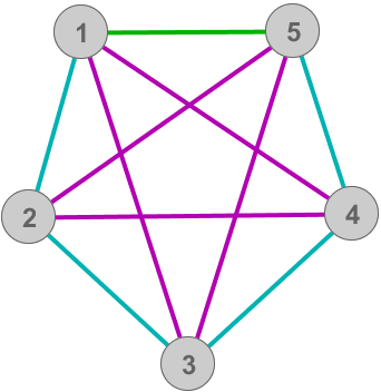
Figure 1: Blue edges denote the semidistance of length $1$, purple edges are of length $4$, while the only green edge is the longest and has the length $20$.

A simple calculation reveals that $(X,d)$ is a $4-$metric space, but it is not a $4-$polygon space since for a finite sequence $(x_{k})_{k=1}^{5}$, $x_{k}:=k$ the constant $\gamma$ has to satisfy:

$$d(x_{1},x_{5})=20\leqslant\gamma\cdot\sum_{k=1}^{4}d(x_{k},x_{k+1})=4\gamma.$$

This proves that $\gamma\geqslant 5.$ After a few more easy computations one can be convinced that $\gamma=5.$

From a theoretical standpoint, the existence of constants $\beta$ and $\gamma$ suffices to construct an “abstract mathematical theory”. However, in practice it is preferable to know the precise values of these constants, hence the need for an algorithm enabling the computation of $\beta$ and $\gamma$ in a reasonable time-scope. We will come back to this issue once we discuss optimization and complexity theory in Section 3.

2 Graph theory through the lenses of semimetric spaces

We have already defined the elementary concepts of semimetric theory. It is time we invoked the crucibles of graph theory and investigate their interplay with the notions of $\beta-$metric and $\gamma-$polygon spaces intoduced earlier. An additional advantage of our concise review is that we lay down the notational convention used in the sequel. We commence with the definition of a graph:

Definition 3.

A pair $G:=(V,E)$ is called a graph if $V$ is a finite, nonempty set and

$$E\subset\{\{x,y\}\ :\ x,y\in V,\ x\neq y\}.$$

The elements of $V$ and $E$ are called vertices and edges, respectively.

A weighted graph is a pair $(G,\omega)$, where $G=(V,E)$ is a graph, $E\neq\emptyset$ and $\omega:E\longrightarrow(0,+\infty)$ is a positive function, called the weight.

A couple of remarks concerning this definition are in order. First off, it is usually convenient to utter the phrase “Let $G$ be a graph” and then refer to the vertex and edge set of $G$ as $V(G)$ and $E(G)$, respectively. This is a convention that we adhere to in the sequel. Furthermore, those acquainted with the graph terminology will surely recognize our graphs to be undirected and simple. “Undirectedness” of a graph means that the edges are not oriented, i.e. every edge is a set $\{x,y\}$ rather than an ordered pair $(x,y).$ On the other hand “simplicity” means that the graph contains no “loops” (i.e. edges of the form $\{x,x\}$) or multiedges (i.e. $E$ is a set and not a multiset). The need for multiedges and multigraphs will arise, however, towards the end of the paper, hence we take the liberty of including the formal definition of these objects:

Definition 4.

A pair $\mathbb{G}:=(V,\mathbb{E})$ is called a multigraph if $V$ is a finite, nonempty set and

$$\mathbb{E}\subset\bigg{\{}(k,\{x,y\})\ :\ x,y\in V,\ x\neq y,\ k\in\mathbb{N}_{0}\bigg{\}}.$$

The elements of $\mathbb{E}$ are called multiedges (while the elements of $V$ are still called vertices). A weighted multigraph is a pair $(\mathbb{G},\omega)$, where $\mathbb{G}=(V,\mathbb{E})$ is a multigraph, $\mathbb{E}\neq\emptyset$ and $\omega:\mathbb{E}\longrightarrow(0,+\infty)$ is a positive function, called the weight.

It goes without saying that the index $k$ in the above definition is used to distinguish different edges connecting the same pair of vertices. More importantly, the way we define a weight (on a graph or a multigraph) slightly deviates from the ones existent in the literature - this is because we assume $\omega$ to be a positive function.

Having defined what we mean by the term “graph” let us proceed with a series of related concepts:

Definition 5.

Let $G$ be a graph.

• Graph $F$ is called a subgraph of $G$ if $V(F)\subset V(G)$ and $E(F)\subset E(G)$. We denote this situation by writing $F\subset G$.

• Graph $P$ is called a path if vertices of $P$ can be arranged in a sequence so that two vertices are adjacent if and only if they are consecutive in this sequence.

• Graph $C$ is called a cycle if the removal of any edge in $C$ turns it into a path. If $G$ does not contain any cycle as a subgraph, then it is called a acyclic graph.

• Subgraph $H\subset G$ is called a Hamiltonian path/cycle if it is a path/cycle visiting each vertex of $G$ exactly once. The family of all Hamiltonian cycles in $G$ is denoted by $\mathfrak{h}(G).$

A graph $G$ whose family of Hamiltonian cycles is nonempty is sometimes called a Hamiltonian graph. The definition of path allows us to introduce one more important notion.

Definition 6.

A graph $G$ is said to be connected if for any pair of vertices $x,y\in V(G)$ there exists a path $P\subset G$ such that $x,y\in V(P)$.

The notion of a subgraph introduced in Definition 5 is inherently independent of the weight function (if such exists) on graph $G$. However, if $\omega$ is a weight on $G$ and $F$ is a subgraph of $G$, then $(F,\omega|_{E(F)})$ is a weighted graph and $\omega|_{E(F)}$ is called an induced weight. Furthermore, it is often convenient to speak of a weight of a subgraph (or the whole graph itself), which we define as

$$\omega(F):=\sum_{e\in E(F)}\omega(e).$$

It is hard to deny that this definition is a slight abuse of notation - after all, we use the same symbol “$\omega$” to weigh both edges and a subgraph. Formally this is a mistake since edges and subgraphs are objects from different “categories” - edges are unordered pairs of elements while subgraphs are pairs of vertex and edge sets. However, we believe that such a small inconsistency should not lead to any kind of misunderstanding (one reason being that we use capital letters for graphs and subgraphs and minuscule letters for edges).

We have now gathered all the necessary ingredients to formulate the Travelling Salesperson Problem (or TSP for short), which is the focal point of our paper:

For a weighted graph $(G,\omega)$ with $\mathfrak{h}(G)\neq\emptyset$ find a Hamiltonian cycle $H$ with minimal weight.

Travelling salesperson problem is one of the most famous mathematical puzzles and a detailed account of its history is far beyond the scope of this paper. Instead, we recommend just a handful of sources - for an indepth discussion on both history and possible attempts at solving this problem see: [5, 28, 39, 42, 52, 58, 72, 75, 78].

Our formulation of the TSP requires the weighted graph $G$ to satisfy $\mathfrak{h}(G)\neq\emptyset.$ This is fairly obvious, because if there is no Hamiltonian cycle it is impossible to look for one with minimal weight! That being said, in the sequel we will usually consider the TSP on a complete weighted graphs, which trivially satisfy the condition $\mathfrak{h}(G)\neq\emptyset.$ The reason we may restrict our attention to complete graphs is that it is always possible to define $\omega(\{x,y\})$ as a “sufficiently large value” for edges $\{x,y\}$ which are not in the original graph $G$. A formal result which encapsulates this intuition is provided below:

Theorem 2.

(well-known in mathematical folklore)
Let $(G,\omega_{G})$ be a graph with $n:=|V(G)|\geqslant 3$ vertices. There exists a complete weighted graph $(K_{n},\omega)$ such that:

1. $G$ is a subgraph of $K_{n}$ and $\omega|_{G}=\omega_{G}$.

2. If $H$ is a minimal Hamiltonian cycle in $(K_{n},\omega)$ and $\omega$ is a subgraph extension of $\omega_{G}$, then exactly one of the following holds:

   • $\omega(H)\leqslant\omega(G)$ and $H$ is a minimal Hamiltonian cycle in $G$ as well, or

   • $\omega(H)>\omega(G)$ and $G$ does not admit any Hamiltonian cycle.

Proof.

Let $K_{n}$ be a complete graph on $n$ vertices of the graph $G$ and let the weight $\omega$ on $K_{n}$ be defined with the formula:

$$\omega(\{x,y\}):=\begin{cases}\omega_{G}(\{x,y\}),&\text{if }\{x,y\}\in E(G),\\ \sum_{e\in E(G)}\ \omega_{G}(e),&\text{otherwise. }\\ \end{cases}$$ (6)

Immediately it follows that $G$ is a subgraph of $K_{n}$ and $\omega|_{G}=\omega_{G},$ which is the first part of the theorem.

For the second part let $\omega$ be a subgraph extension of $\omega$ and let $H$ be a minimal Hamiltonian cycle in $(K_{n},\omega).$ We divide our reasoning into two separate cases:

• Suppose that $\omega(H)\leqslant\omega(G).$ Definition (6) implies that $H$ cannot contain any edge which is not in $E(G),$ since otherwise we would have

  $$\omega(H)>\omega(G)=\sum_{e\in E(G)}\ \omega(e).$$

  Furthermore, there cannot exist a Hamiltonian cycle $H^{\prime}$ on $(G,\omega_{G})$ such that $\omega(H^{\prime})<\omega_{G}(H),$ simply because that would prevent $H$ from being a minimal Hamiltonian cycle on $(K_{n},\omega).$ Therefore we have to conclude that $H$ is a minimal Hamiltonian cycle on $(G,\omega_{G}).$

• Suppose that $\omega(H)>\omega(G).$ If there existed a minimal Hamiltonian cycle $H^{\prime}$ on $G$ then we would have

  $$\omega(H^{\prime})\leqslant\omega(G)<\omega(H).$$

  This contradicts the fact that $H$ is a minimal Hamiltonian cycle in $K_{n}$ (since there is a cycle with smaller weight, namely $H^{\prime}$), which concludes the proof.

∎

In the light of the above, we may restrict our focus to the case where the graph in the formulation of the TSP is a complete weighted graph i.e., $G=(K_{n},\omega)$. For such graphs we are able to impose the semimetric structure on $V(G)$ as follows:

$$d(x,y):=\begin{cases}\omega\left(\{x,y\}\right),&\text{ where }x\neq y;\\ 0,&\text{ where }x=y.\end{cases}$$ (7)

This allows us to define some particular subclasses of complete weighted graphs as follows:

Definition 7.

A graph $G=(K_{n},\omega)$ is called

• a metric graph if $d$ is a metric on $V(G)$;

• a $\beta-$metric graph if $d$ satisfies (1);

• a $\gamma-$metric graph if $d$ satisfies (2).

Depending on the additional conditions imposed on the graph weights, we can obtain more specific variants of TSP. In particular, when $d$ satisfies the triangle inequality, we can talk about the metric TSP (cases where particular instance is considered on a plane are sometimes referred to as Euclidean Traveling Salesman Problem). While it might seem the metric TSP should be much easier to solve, it was shown by Christos Papadimitriou that even in the case of Euclidean metric setting, the Traveling Salesman Problem remains NP-hard. It is therefore reasonable to consider approximation algorithms as a valuable asset in the array of techniques designed for coping with such problems.

3 Optimization and complexity theory

We believe that our paper might be of interest to both researchers in algorithm-related branches as well as those working wiht various generalizations of metric spaces. Bearing that in mind, the focal point of the current subsection is a brief summary of fundamental notions and facts in optimization and complexity theory.

We start off with the idea of “optimization problem” itself:

Definition 8.

Let $X$ be a nonempty, finite set and let $f:X\longrightarrow(0,+\infty)$ be an arbitrary function. A problem of finding an element $x^{*}\in X$ which satisfies

$$f(x^{*})=\min_{x\in X}f(x),$$ (8)

is called an optimization problem.

Set $X$ and function $f$ in the optimization problem are called the search space and the target function, respectively. Furthermore, every element satisfying (8) is said to be an optimal solution (there might be more than one such element), while the elements of $X$ are referred to as feasible solutions.

At first glance, solving a optimization problem on a finite set seems trivial. Why not go through all elements of $X$ one by one, checking the values $f(x)$ and choosing the minimal one? Well, in theory this is a perfectly valid approach but in practice it is too cost-inefficient (takes too much time and memory space). Take, for instance, the Travelling Salesperson Problem, which is an optimization problem - for a given weighted graph $(G,\omega)$ it suffices to put $X:=\mathfrak{h}(G)$ and $f:=\omega$. If $G=K_{61}$ then there are $\frac{1}{2}\cdot 60!$ Hamiltonian cycles, which is more than the number of atoms in the observable universe (roughly $10^{80}$ particles)! Without divine intervention solving such a gargantuan problem is simply inconceivable.

Let us pause for a moment and see how the tables have turned. What seemed like an innocuous task now appears as an insurmountable hinderance. Luckily, not all is lost. There is a way out but we need to allow for a small “hustle”: instead of searching for the optimal solution, we look for an approximate solution, which is (in some sense) “good enough”. More than that, we usually look for an approximation method (rather than a single approximate solution for a fixed optimization problem), i.e. an algorithm which can be applied to a whole family of optimization problems:

Definition 9.

Let $s\geqslant 1$ and let $\mathcal{P}$ be a set of indices for a family of optimization problems with target functions $f_{p}:X_{p}\longrightarrow(0,+\infty).$ A function $\mathfrak{a}:\mathcal{P}\to\bigcup_{p\in\mathcal{P}}X_{p}$ is called an $s$-optimal approximation method for $\mathcal{P}$ if for every $p\in\mathcal{P}$ we have

$$\mathfrak{a}(p)\in X_{p}\hskip 11.38092pt\text{and}\hskip 11.38092pt\frac{f_{p}\left(\mathfrak{a}(p)\right)}{f_{p}\left(x^{*}_{p}\right)}\leqslant s,$$

where $x_{p}^{*}$ is some optimal solution of the $p-$th optimization problem.

With such terminology at our disposal, we can say that the rest of the paper is devoted to finding $s$-optimal approximation methods for the Travelling Salesman Problem. We will focus on two methods:

• Minimal spanning tree method on metric and $\gamma-$polygon graphs (Section 4);

• Christofides algorithm on $\gamma-$polygon graphs (Section 6).

Before we proceed with the analysis of these approximation methods, let us close the current section with a couple of words regarding the basic principles of time complexity of algorithms. Please bear in mind, however, that our exposition is extremely rudimentary - we refer an inquisitve Reader to the vast literature on the subject, see the books of Oded Goldreich [46, Section 1.2.3.4] and [47, Section 1.3.5], as well as [6, 7, 33, 70].

Let $\mathcal{P}$ be a set of indices for a family of optimization problems and let $\mathcal{M}:\mathcal{P}\longrightarrow\mathbb{N}$ be a function, which to every $p\in\mathcal{P}$ assigns the number of memory units (within the scope of the discussed model of computation, say the traditional Turing machine) used to describe the $p-$th problem. We say that an algorithm $\mathfrak{a}:\mathcal{P}\longrightarrow\mathbb{R}$ has computational (time) complexity at most $F_{\mathfrak{a}}:\mathbb{N}\longrightarrow\mathbb{N}$ if there exists a constant $\alpha\geqslant 0$ such that for $p-$th problem the algorithm $\mathfrak{a}$ requires no more than $\alpha\cdot F_{\mathfrak{a}}(\mathcal{M}(p))$ units of computation. Whenever this holds, we say that $\mathfrak{a}$ can be executed in time $\mathcal{O}(F_{\mathfrak{a}}(n)).$

We are now in position to go back to the problem that we left off after Theorem 1 concerning the computation of constant $\beta$ for a finite semimetric space. A naive brute-force approach which calculates every quotient of the form $\frac{d(x,z)}{d(x,y)+d(y,z)}$ and picks the one with the heighest value has time complexity $\mathcal{O}(n^{3})$, where $n$ is the cardinality of the semimetric space $X$. The problem of finding $\gamma$ is slightly more nuanced, but (surprisingly) has the same time-complexity:

Theorem 3.

Let $(X,d)$ be a finite semimetric space consisting of $n$ distinct points. The constant $\gamma$ such that $(X,d)$ satisfies the $\gamma$-polygon inequality can be found with time-complexity $\mathcal{O}(n^{3})$.

Proof.

Let $G:=(K_{n},\omega)$ be a complete weighted graph, where $\omega\left(\{x,y\}\right):=d(x,y)$ for all pairs of distinct $x,y\in V(K_{n})=X.$ On this graph we execute the Floyd-Warshall shortest paths algorithm, which returns a function $D:X\times X\longrightarrow[0,\infty),$ where $D(x,y)$ denotes the length of the shortest path between points $x$ and $y$, i.e.

$$D(x,y):=\min\left\{\sum_{k=1}^{n-1}d(x_{k},x_{k+1})\ :\ n\in\mathbb{N},\ x_{1}=x,\ x_{n}=y,\ x_{k}\in X\text{ for }k\leqslant n\right\}.$$

The execution of the algorithm has time complexity $\mathcal{O}(n^{3})$.

Next, we define a function $\Gamma:\{(x,y)\ :\ x,y\in X,\ x\neq y\}\longrightarrow[0,\infty)$ by the formula

$$\Gamma(x,y):=\frac{d(x,y)}{D(x,y)}.$$

Since each edge of $G$ has positive weight, then $\Gamma$ is well-defined. Furthermore, $\Gamma(x,y)\geqslant 1$ since the shortest path between any distinct elements $x$ and $y$ is no longer than the edge $\{x,y\}$ - in other words it must be the case that $D(x,y)\leqslant d(x,y)$.

Finally, we observe that

$$\gamma=\max_{(x,y)}\ \Gamma(x,y).$$

Computationally, in order to find the maximum on the right-hand side of the equation we need to check $\frac{n(n-1)}{2}$ values of $\Gamma$ (due to the symmetry $\Gamma(x,y)=\Gamma(y,x)$). Therefore, the time-complexity of the whole procedure (including the Floyd-Warshall algorithm) is $\mathcal{O}(n^{3}).$ ∎

4 Minimal spanning tree method on metric, $\beta-$metric and $\gamma-$polygon graphs

As far as we are aware, the first application of $\beta$-metric spaces to combinatorial optimization problems dates back to 1994 and the paper by Bandelt, Crama and Spieksma [11], where the authors use the relaxed version of the triangle inequality to construct approximation algorithms for multi-dimensional assignment problems with decomposable costs. The idea of using $\beta-$metric spaces swiftly gained recognition and it wasn’t long before consecutive authors applied $\beta-$metric inequality to the Travelling Salesperson Problem - see [3, 4, 12, 65, 66]. On the hand, to the best of our knowledge, there are no known results in the literature which employ the $\gamma-$polygon inequality in the context of the Travelling Salesperson Problem.

The crucial concept with which we will be preoccupied throughout this section is that of a minimal spanning tree:

Definition 10.

Let $G$ be a graph.

• A connected, acyclic subgraph $T\subset G$ is called a tree.

• A tree $T$ which satisfies $V(T)=V(G)$ is called a spanning tree of $G$.

• The family of all spanning trees of $G$ is denoted by $\mathcal{S}(G)$.

If $(G,\omega)$ is a weighted graph, then any tree $T\in\mathcal{S}(G)$ which satisfies

$$\omega(T)=\min_{T^{\prime}\in\mathcal{S}(G)}\omega(T^{\prime})$$

is called a minimal spanning tree (or MST for short).

Before we proceed with laying the basic outline of the minimal spanning tree method method let us introduce the concept of a tree traversal . This notion will significantly facilitate our future discussion:

Definition 11.

Let $G$ be a graph.

• An $n$-element sequence of vertices $(x_{1},\dots,x_{n})$ such that $\{x_{k},x_{k+1}\}\in E(G)$ for every $k<n$ is called a walk (on graph $G$).

• A walk on graph $G$ is said to be closed if it starts and ends at the same vertex.

If $T$ is a tree on graph $G$, then any walk on $T$ which visits its every edge exactly twice is called a tree traversal.

We are now in position to formulate the general framework of the minimal spanning tree method (or the MST method for short):

step 1.   

Given a complete weighted graph $G:=(K_{n},\omega)$ we find (one of) its minimal spanning tree(s) $T$.

step 2.   

Via a depth-first search (or DFS for short) on $T$ we construct a tree traversal (which depends on the root of the algorithm).

step 3.   

We perform a shortcutting procedure on the tree traversal (from the previous step) to obtain a Hamiltonian cycle on $G$.

The first two steps are widely recognized and can be found in numerous sources. Therefore, we will only discuss step 3, i.e., the shortcutting procedure, which is relatively less known.

Let $G:=(K_{n},\omega)$ be a complete weighted graph on $n\in\mathbb{N},n\geqslant 3$ vertices and let $T$ be a minimal spanning tree of $G$. We choose an arbitrary vertex $x_{1}\in V(T),$ which we refer to as the root of the tree, and perform a DFS to obtain a tree traversal $(x_{1},\ldots,x_{2n-1}).$ Next, we define $(y_{1},\dots,y_{n},y_{n+1})$ as the sequence obtained from $(x_{1},\dots,x_{2n-1})$ by the shortcutting procedure:

$$y_{i}:=\begin{cases}x_{1},&i=1,n+1,\\ x_{m(i)},&i=2,\ldots,n,\end{cases}$$ (9)

where

$$m(i):=\min\bigg{\{}j:i\leqslant j\leqslant 2n-1\ \text{and}\ x_{j}\not\in\{x_{1},\dots,x_{j-1}\}\bigg{\}}.$$

At first glance, the definition (9) may seem a bit daunting. However, there is a simple recipe for obtaining the shortcut $(y_{1},\dots,y_{n},y_{n+1}).$ We go through the elements of $(x_{1},\dots,x_{2n-1})$ one by one and cross out every “repetition” (an element that has already appeared earlier in the sequence) except for $x_{2n-1}$ which is the same as $x_{1}$. In the “shortcutted” sequence $C_{T}:=(y_{i})_{i=1}^{n+1}$ every vertex (except for the root $x_{1}$) appears precisely once (after all, we did cross out all repetitions other than $x_{1}=x_{2n-1}$). It is easy to see that $C_{T}$ is in fact a Hamiltionian cycle on $G,$ which we call a $(T,x_{1})-$shorcut of the graph $G$.

In order to reinforce our intuition, let us consider the following example of the shortcutting procedure:

Example 2.

Consider a complete graph $K_{6}$ with vertices $V:=\{1,\dots,6\}$. Let $T$ be a spanning tree with the following set of edges

$$E(T)=\bigg{\{}\{1,2\},\{2,3\},\{3,4\},\{3,5\},\{5,6\}\bigg{\}}.$$

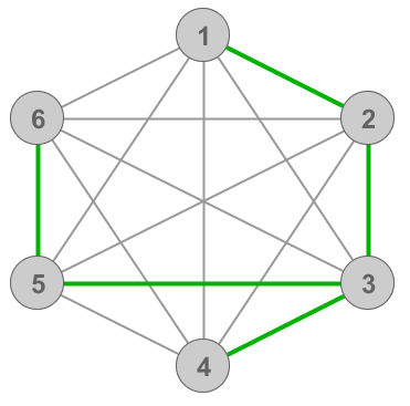
Figure 2: Spanning tree $T$ on the complete graph $K_{6}$.

Let us consider a tree traversal starting at the vertex $1$ (the root of the tree $T$). We subsequently visit the vertices $2$ and $3$ - then we are forced to make a choice. Let us proceed with vertices $5$ and $6$. We then backtrack to $3$ and visit $4$. After retracing our steps back to $1$ we obtain a tree traversal $R_{1}$:

$$R_{1}:=(1,2,3,5,6,5,3,4,3,2,1).$$

Performing the shortcutting procedure we remove those vertices which appear multiple times (except for the final one) in the sequence $R_{1}.$ The final result is the Hamiltonian cycle

$$C_{1}:=(1,2,3,5,6,4,1).$$

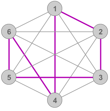
Figure 3: Hamiltonian cycle $C_{1}$.

In order to see that $C_{1}$ is not the only possible $(T,1)-$shortcut, we note that it not mandatory to choose $5$ after $3$. We may as well choose $4$, backtrack to $3$, and only then go to $5$ and $6$ This results in a tree traversal

$$R_{2}:=(1,2,3,4,3,5,6,5,3,2,1).$$

Applying shortcutting procedure to $R_{2}$ yields a different Hamilton cycle

$$C_{2}:=(1,2,3,4,5,6,1).$$

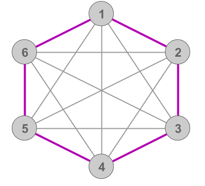
Figure 4: The Hamiltonian cycle $C_{2}$.

5 Performance of the MST method

We already know that the MST method returns a Hamiltonian cycle for a given graph $G$. It is high time we examined how close this cycle is to being a solution to the TSP. To this end we compare the weights of the following two subgraphs of $G$: the optimal solution to the TSP $C^{*}$ and the minimal spanning tree $T$. In fact, we have the following inequality:

$$\omega(T)\leqslant\omega(C^{*}).$$ (10)

The proof of this fact can be shortened to a simple observation that removing a single edge from $C^{*}$ leaves us with some spanning tree $T^{*}$, whose cost is (by definition of MST) bounded from below by $\omega(T)$.

The theorem below addresses this issue under the assumption that the graph is metric:

Theorem 4.

Let $(K_{n},\omega)$ be a complete, metric graph, $T$ be its minimal spanning tree and let $x\in V(T)$. Every $(T,x)-$shortcut $S$ satisfies

$$\omega(S)\leqslant 2\omega(T)\leqslant 2\omega(C^{*}).$$

Proof.

Let $(x_{k})_{k=1}^{2n-1}$ be a tree traversal for $T$ and let $(y_{k})_{k=1}^{n+1}$ denote the elements in the $(T,x)-$cycle $S$. For every $i\leqslant n$ we have

$$\begin{split}d(y_{i},y_{i+1})&=d(x_{m(i)},x_{m(i+1)})\leqslant d(x_{m(i)},x_{m(i)+1})+d(x_{m(i)+1},x_{m(i+1)})\\ &\leqslant\ldots\leqslant\sum_{j=m(i)}^{m(i+1)-1}d(x_{j},x_{j+1}),\end{split}$$ (11)

which implies

$$\omega(S)=\sum_{i=1}^{n}d(y_{i},y_{i+1})\leqslant\sum_{i=1}^{n}\sum_{j=m(i)}^{m(i+1)-1}d(x_{j},x_{j+1})\leqslant\sum_{k=1}^{2n-2}d(x_{k},x_{k+1})=2\omega(T).$$

This concludes the proof. ∎

In the language of optimization theory, Theorem 4 says that the MST method constructs a $2-$optimal approximation for the TSP on a metric graph. The fact that the graph is metric is crucial, as the triangle inequality is used (repeatedly) in (11).

Our next goal is to prove a counterpart of Theorem 4 in the case of $\gamma-$polygon graphs.

Theorem 5.

Let $(K_{n},\omega)$ be a complete, $\gamma-$polygon graph and let $T$ be its minimal spanning tree rooted at vertex $x_{1}$. Every $(T,x_{1})-$shortcut $S$ satisfies

$$\omega(S)\leqslant 2\gamma\omega(T)\leqslant 2\gamma\omega(C^{*}).$$ (12)

Proof.

Again, as in Lemma 4 let $(x_{k})_{k=1}^{2n-1}$ be a tree traversal for $T$ and let $S=(y_{k})_{k=1}^{n+1}$ be its $(T,x_{1})-$shortcut. Performing an analogous reasoning to (11) we have

$$\forall_{i=1,\ldots,n}\ d(y_{i},y_{i+1})=d(x_{m(i)},x_{m(i+1)})\stackrel{{\scriptstyle\eqref{polygonalinequality}}}{{\leqslant}}\gamma\sum_{j=m(i)}^{m(i+1)-1}d(x_{j},x_{j+1}).$$ (13)

Consequently, we obtain

$$\omega(S)=\sum_{i=1}^{n}d(y_{i},y_{i+1})\stackrel{{\scriptstyle(\ref{bmetric_case_assumption})}}{{\leqslant}}\gamma\sum_{i=1}^{n}\sum_{j=m(i)}^{m(i+1)-1}d(x_{j},x_{j+1})\leqslant\gamma\sum_{k=1}^{2n-2}d(x_{k},x_{k+1})\leqslant 2\gamma\omega(T),$$

which concludes the proof. ∎

In the language of optimization theory, Theorem 12 says that our MST method constructs a $2\gamma-$optimal approximation for the TSP. It is natural to examine how the estimate (12) places amongst other results of this kind known in the literature. As far as we are aware, the idea of using $\gamma-$polygon structure of a given graph is a new insight and has not been explored thus far. Instead, researchers focused on $\beta-$metric structure and arrived at four approximation methods, which are most popular in the field. The first one is the $\frac{3\beta^{2}+\beta}{2}-$optimal approximation method, which was devised by Andreae, Bandelt [3] in 1995. This method is nowadays only of historical value since it was improved (in 2001) by Andreae himself to $(\beta^{2}+\beta)$-approximation algorithm [4]. In 2000 Bender and Chekuri [12] constructed a $4\beta$-optimal approximation method while Böckenhauer, Hromkovič, Klasing, Seibert and Unge came up with a $\frac{3\beta^{2}}{2}-$approximation method in 2002. The discussion “which approximation technique is better?” can be best summarized by the following plot:

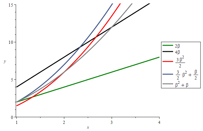
Figure 5: Plot depicting the curves of the approximation constants of the discussed methods.

For instance, one can see that the $\frac{3\beta^{2}}{2}-$optimal approximation method (the red curve) is worse than $(\beta^{2}+\beta)-$optimal approximation method (drawn with light gray colour) for $\beta>2$ but it is better for $\beta<2$.

Where is the estimate (12) situated amongst these optimal approximations using the $\beta-$metric structure of a graph? In order to answer that question we need to have some kind of relation between $\beta$ and $\gamma.$ Obviously, as we remarked earlier we have $\gamma\geqslant\beta,$ but we also need some upper bound on $\gamma$ in terms of $\beta$. We focus our attention on a class of graphs where $\gamma\in[\beta,2\beta)$ and $\beta\geqslant 3.$ These conditions are not very restrictive and Example 1 provides an instance of a graph belonging to such a class. The crucial observation is the if $\gamma\in[\beta,2\beta)$ and $\beta\geqslant 3$ then

$$2\beta\leqslant 2\gamma<4\beta\leqslant\beta^{2}+\beta<\frac{3}{2}\beta^{2}<\frac{3\beta^{2}+\beta}{2}.$$

This means that there exists a large class of graphs for which our estimate (12) is better than anything known in the literature. Furthermore, the class we are discussing is not some “secretive ensemble”. Given a weighted graph it suffices to compute its $\beta$ and $\gamma$ (which can be done relatively efficiently as proven by Theorem 3) and check two conditions: $\beta>3$ and $\gamma<2\beta$. If both of them are true then the application of estimate (12) is highly recommended.

To close off the current section, we will show that the constant $2\gamma$ is in a sense “the best possible” constant in the MST method (unless we modify our approach in the next section). More formally, we show for any $\varepsilon>0$ there exists a complete, weighted graph $(K_{n},\omega_{n})$ such that

$$\omega_{n}(S)>(2\gamma-\varepsilon)\omega_{n}(T).$$

Example 3.

Fix $\gamma\geqslant 1$ and let $(K_{n},\omega_{n})$ be a complete graph consisting of $n$ distinct vertices $x_{1},\dots,x_{n}$, where

$$\omega_{n}\left(\{x_{i},x_{j}\}\right):=\begin{cases}1,&i=1,\ j>1\\ 2\gamma,&i,j>1,\ i\neq j.\end{cases}$$

It is easy to see that there exists exactly one minimal spanning tree $T$ in such a graph, namely the one with

$$E(T)=\bigg{\{}(x_{1},x_{k})\ :\ k\in\{2,\dots,n\}\bigg{\}}.$$

Since the weight of each edge of $T$ is equal to $1$, we have $\omega_{n}(T)=n-1$.

Performing a depth-first search algorithm on $T$ (starting at $x_{1}$) we obtain a tree traversal:

$$W:=(x_{1},x_{2},x_{1},x_{3},x_{1},\dots,x_{n},x_{1}).$$

Next, the shortcutting procedure yields a $(T,x_{1})-$shortcut

$$S:=(x_{1},x_{2},x_{3},\dots,x_{n},x_{1})$$

with

$$\omega_{n}(S)=1+(n-2)\cdot 2\gamma+1=2\cdot(1+\gamma(n-2)).$$

It remains to note that

$$\lim_{n\rightarrow\infty}\ \frac{\omega_{n}(S)}{\omega_{n}(T)}=\lim_{n\rightarrow\infty}\ \frac{2\cdot(1+\gamma(n-2))}{(n-1)}=2\gamma.$$

6 Christofides algorithm on $\gamma-$polygon graphs

In the previous section we laid out a $2\gamma-$approximation method for the TSP (constructing a $(T,x)-$-shortcut from a MST $T$ and the root $x$) and one may wonder whether we can do any better than that? Luckily, the answer is “yes!” and our final section of the paper is devoted to presenting the details of this refined approach.

The core idea of our method comes from the work of Christofides, who came up with a $\frac{3}{2}-$optimal approximation method for the class of metric graphs. Our goal in the current section is to extend the scope of his method to the class of $\gamma$-polygon graphs, which is (as far as we are aware) a novelty in the field.

To begin with, we recall a couple of definitions, which are vital in understanding what follows:

Definition 12.

Let $(V,E)$ be a graph. The number of edges incident to $x\in V$, i.e.

$$\deg(x):=\left|\left\{\{x,y\}\in E\ :\ y\in V\right\}\right|,$$

is called the degree of vertex $x.$

Definition 13.

Let $(V,E)$ be a graph. A set of edges $E_{M}\subset E$ is called a matching, if no two edges of $E_{M}$ share a common vertex, i.e. for any two edges $\{x_{1},y_{1}\},\{x_{2},y_{2}\}\in E_{M}$ we have

$$\{x_{1},y_{1}\}\cap\{x_{2},y_{2}\}=\emptyset.$$

If each vertex has an incident edge in $E_{M}$, i.e.

$$\forall_{x\in V}\ \exists_{y\in V}\ \{x,y\}\in E_{M},$$

then the matching $E_{M}$ is said to be a perfect matching.

Of course every matching can be viewed as a subgraph of the original graph $(V,E)$– $E_{M}$ is the “new” set of edges and the endpoints of these edges form the “new” set of vertices. The last definition that we need for the sequel is the following:

Definition 14.

Let $(G,\omega)$ be a weighted graph and let $M\subset G$ be its perfect matching. We say that $M$ is a minimum-weight perfect matching if for any other perfect matching $M^{\prime}\subset G$ we have $\omega(M)\leqslant\omega(M^{\prime})$.

At this point we have gathered all the necessary concepts to revisit the approximate solution for the TSP devised by Christofides. Given a complete weighted graph $(K_{n},\omega)$ we follow the steps:

step 1.   

Find the minimal spanning tree $T$ of $G$ (using Boruvka’s, Prim’s or Kruskal’s algorithm for instance).

step 2.   

Let $V_{odd}$ be the set of all odd vertices (i.e., vertices with odd degrees) of $T$. Let $F$ be a weighted subgraph induced on $G$ by $V_{odd}$.

step 3.   

Find a minimum-weight perfect matching in $F$ and denote it by $M$. This can be done by applying the original Edmonds’ blossom algorithm or one of its subsequent versions.

step 4.   

Find an Eulerian walk $W$ in the multigraph $\mathbb{G}=(V(T),\mathbb{E}),$ where

$$\mathbb{E}=\bigg{\{}(0,e)\ :\ e\in E(T)\bigg{\}}\cup\bigg{\{}(1,e)\ :\ e\in E(M)\bigg{\}}.$$

step 5.   

Perform shortcutting procedure on $W$, thus obtaining a Hamiltonian cycle $C$.

It might not be obvious at first glance why the multigraph $\mathbb{G}$ constructed in fourth point of this algorithm necessarily has an Eulerian walk. These doubts are dispelled by the following lemma:

Lemma 6.

If each vertex of a connected (multi-)graph has an even degree, then there exists an Eulerian cycle in this (multi-)graph.

As far as time complexity of Christofides’ algorithm is concerned, we remark that in the worst case scenario we have to look for a minimum-weight perfect matching in the whole graph $G$ (when performing point 3.). This is arguably the choke-point of the whole procedure. The minimum-weight perfect matching can be found with the use of Gabow’s algorithm with time complexity $\mathcal{O}(|V(G)|^{3}),$ although there are more efficient methods if all weights are natural numbers (which we do not assume in this paper). The time complexity of Gabow’s algorithm also sets the complexity for the whole procedure.

In the case of metric graphs, Christofides proved that the Hamiltonian cycle $C$ returned by his algorithm satisfies $\omega(C)\leqslant\omega(T)+\omega(M)$. Next, Christofides established the inequality

$$\omega(M)\leqslant\frac{1}{2}\omega(C^{*})$$ (14)

where $C^{*}$ is an optimal solution for the TSP. Finally, using the inequality $\omega(T)\leqslant\omega(C^{*})$, he arrived at the conclusion that $C$ is a $\frac{3}{2}$-optimal approximation.

Let us emphasize that Chistofides’ reasoning (and the constant $\frac{3}{2}$) hinges upon the metricity of the graph. Our objective now is to extend this method to a more general setting of $\gamma-$polygon graphs. We carry out the first 3 steps exactly as we did in the metric case. At the end of step 3 we have constructed a minimal-weight perfect matching, but (14) may not hold since the graph need no longer be metric! So what is the couterpart of bound (14) in the $\gamma-$polygonal case? The answer is given by the following lemma:

Lemma 7.

Let $C^{*}$ be the optimal solution for TSP in a complete weighted $\gamma-$polygon graph $G$. Let $F$ be any complete subgraph of $G$ having an even number of vertices. If $M$ is a minimum-weight perfect matching in $F$, then

$$\omega(M)\leqslant\frac{\gamma}{2}\omega(C^{*}).$$

Proof.

Let $C^{*}:=(y_{1},\dots,y_{n},y_{1})$, where $y_{1}$ is some arbitrarily chosen vertex from $F$. Let $z_{1}:=y_{1}$ and $C_{F}:=(z_{1},z_{2},\ldots,z_{m},z_{1})$ be an unique enumeration of vertices of $F$ such that $z_{i}$ preceeds $z_{j}$ in $C^{*}$ whenever $i<j$.

Notice that

$$\forall_{i=1,\ldots,m}\ \omega(\{z_{i},z_{i+1}\})\leqslant\gamma\sum_{j=k_{i}}^{k_{i+1}-1}\omega(\{y_{j},y_{j+1}\}),$$ (15)

where $y_{k_{i}}=x_{i}$ and $y_{k_{i+1}}=x_{i+1}$ (and $x_{m+1}:=x_{1}$). This leads us to the conclusion that

$$\omega(C_{F})\leqslant\gamma\omega(C^{*}).$$ (16)

Next, we split the cycle $C_{F}$ into two matchings by “alternating the edges”, i.e.

$$\begin{split}M_{1}&:=\left(V(F),\left\{\{z_{1},z_{2}\},\{z_{3},z_{4}\},\dots,\{z_{m-1},z_{m}\}\right\}\right),\\ M_{2}&:=\left(V(F),\left\{\{z_{2},z_{3}\},\{z_{4},z_{5}\},\dots,\{z_{m},z_{1}\}\right\}\right).\end{split}$$

Obviously we have $\omega(M_{1})+\omega(M_{2})=\omega(C_{F}),$ which implies that either $\omega(M_{1})\leqslant\frac{\omega(C_{F})}{2}$ or $\omega(M_{2})\leqslant\frac{\omega(C_{F})}{2}$. Either way, if $M$ is the minimum-weight perfect matching then

$$\omega(M)\leqslant\min\left\{\omega(M_{1}),\omega(M_{2})\right\}\leqslant\frac{\omega(C_{F})}{2}\stackrel{{\scriptstyle(\ref{estimateonCF})}}{{\leqslant}}\frac{\gamma}{2}\omega(C^{*}),$$

which concludes the proof. ∎

Next, we proceed with a counterpart of step 4. and mildly modify the Hierholzer algorithm to guarantee that the first edge of the resulting Eulerian cycle is specifically taken from the matching. Let $\mathbb{G}:=((V,\mathbb{E}),\omega)$ be a weighted multigraph, where

• $V(\mathbb{G}):=V(G)=V(T)$;

• $\mathbb{E}(G):=\left\{(0,e)\ :\ e\in E(T)\right\}\cup\left\{(1,e)\ :\ e\in E(M)\right\}.$

Our modified variant of Hierholzer algorithm can be described in the following points:

1. Select arbitrary starting vertex $x_{1}\in V(\mathbb{G})$, which is incident to some edge from $E(M)$. Let $W:=(y_{1})$, where $y_{1}:=x_{1}$. Mark $y_{1}$ as a “recently visited vertex”.

2. Extend the sequence of vertices $W$ in the following way:

   1. select any neighbour $y$ of the “recently visited vertex” connected to it by an “unused” edge in $E(M)$ (if possible) or in $E(\mathbb{G})$ (this is always possible because each vertex in $V(\mathbb{G})$ has even degree).

   2. add $y$ to the sequence $W$. Mark $y$ as the “recently visited vertex” and denote the traversed edge as “used”. If there is an unused edge incident to $y$, go back to step a).

3. If there are any unused edges after this process, start at any vertex $x\in W$ which has at least one neighbour not in $W$. Repeat the procedure described in step 2 obtaining a closed walk $W_{x}.$ Replace the last appearance of $x$ in sequence $W$ with $W_{x}$.

Having obtained an Eulerian walk $W:=(x_{1},\dots,x_{k+1}),\ k=|E(M)|+|E(T)|$ by the means of previously discussed algorithm, we can move to the last, fifth step of our procedure, i.e., shortcutting. This is a rather subtle point. If we were to shortcut in a naive way (as we did in the metric case) then we could cross out the edges from the matching. This, in turn, would cause the error estimate to include the relaxation constant $\gamma$ twice – once in the shortcutting procedure and the second time in the estimation of the total cost of the matching. Since $\gamma$ usually exceeds $1$, we definitely want to avoid having $\gamma^{2}$ in the error estimate.

In order to avoid that obstacle we introduce the following enhanced shortcutting procedure, which results in the Hamiltonian cycle $\tilde{C}_{T}:=(y_{1},\dots,y_{n},y_{n+1})$:

1. Assign $y_{1}:=x_{1}$ and $y_{2}:=x_{2}$. From the construction of $W$ (the Eulerian walk from the previous step) it follows that $\{x_{1},x_{2}\}\in E(M)$. Let $i:=3$ and $j:=3$.

2. While $i\leqslant n$ perform the following steps:

   1. If $x_{j}\notin V(M)$ and it already has appeared in $\tilde{C}_{T}$, increment $j$.

   2. If $x_{j}\notin V(M)$ has not appeared in $\tilde{C}_{T}$ so far, put $y_{i}:=x_{j}$. In such case, increment both $i$ and $j$.

   3. If $x_{j}\in V(M)$, $\{x_{j},x_{j+1}\}\notin E(M)$ and $\{x_{j-1},x_{j}\}\notin E(M)$, increment $j$.

   4. Otherwise, i.e., in the situation where $x_{j}\in V(M)$ and either $\{x_{j},x_{j+1}\}\in E(M)$ or $\{x_{j-1},x_{j}\}\in E(M)$, let $y_{i}:=x_{j}$. Increment both $i$ and $j$.

Notice that these four situations described above not only are mutually exclusive, but they also guarantee that each vertex will appear exactly once in $\tilde{C}_{T}$. In the case where $x_{j}\notin V(M)$, the assignment takes place upon the first encounter of the discussed vertex. In the case where $x_{j}\in V(M)$, the spot in which $x_{j}$ is assigned is unique as well, due to the fact that every vertex in $V(M)$ has a degree in subgraph $M$ equal to $1$. This way the resulting Hamiltonian cycle $\tilde{C}_{T}$ contains all edges from $E(M)$ i.e., no edge from $E(M)$ was erased during the shortcutting procedure.

Theorem 8.

We have

$$\sum_{e\in E(\tilde{C}_{T})\backslash E(M)}\ \omega(e)\leqslant\gamma\omega(T).$$

Proof.

If $e\in E(\tilde{C}_{T})\backslash E(M)$ then $e=\{y_{k},y_{k+1}\}$ for some $y_{k},y_{k+1}\in V(G).$ Furthermore, there exist

$$x_{k_{i}}:=y_{k},\ x_{k_{i}+1},\ \ldots,\ x_{k_{j}}:=y_{k+1}$$ (17)

such that

$$\{x_{k_{i}},x_{k_{i}+1}\},\ldots,\{x_{k_{j}-1},x_{k_{j}}\}\in(E(M)\cup E(T)),$$

because all the $x_{k}$’s are the vertices from the Eulerian walk $W$. Next, we observe that

$$\forall_{l=0,\ldots,k_{j}-k_{i}-1}\ \{x_{k_{i}+l},x_{k_{i}+l+1}\}\not\in E(M),$$

since that would imply that an edge from the perfect matching $M$ was shortcutted, which is impossible. Thus (by the $\gamma-$polygon inequality) we have establish that

$$\forall_{e\in E(\tilde{C}_{T})\backslash E(M)}\ \omega(e)\leqslant\gamma\sum_{l=0}^{k_{j}-k_{i}-1}\ \omega(\{x_{k_{i}+l},x_{k_{i}+l+1}\}).$$ (18)

Observe that for distinct $i,j$ we have that chains of edges defined by (17) are disjoint (this is due to the fact that Eulerian walk $W$ visits every edge in multigraph $\mathbb{G}$ exactly once). As a consequence, on the right-hand side of the inequalities (18) no edge appears more than once for all $e\in E(\tilde{C}_{T})\setminus E(M)$. Finally, we have

$$\sum_{\{y_{k},y_{k+1}\}\in E(\tilde{C}_{T})\backslash E(M)}\ \omega(\{y_{k},y_{k+1}\})\leqslant\gamma\sum_{\{k_{i}\ :\ y_{k}=x_{k_{i}}\}}\sum_{l=0}^{k_{j}-k_{i}-1}\ \omega(\{x_{k_{i}+l},x_{k_{i}+l+1}\})\leqslant\gamma E(T),$$

which ends the proof. ∎

Since $E(M)\subset E(\tilde{C}_{T})$ then

$$\omega(\tilde{C}_{T})=\sum_{e\in E(\tilde{C}_{T})\backslash E(M)}\ \omega(e)+\sum_{e\in E(M)}\ \omega(e)\stackrel{{\scriptstyle Theorem\ \ref{greatheorem},\ Lemma\ \ref{lemma7}}}{{\leqslant}}\gamma\omega(T)+\frac{\gamma}{2}\omega(C^{*})\leqslant\frac{3\gamma}{2}\omega(C^{*}).$$

Thus we have reached the climax of our paper:

Theorem 9.

Let $(K_{n},\omega)$ be a complete $\gamma$-polygon graph. There exists a $\frac{3\gamma}{2}$-approximation to the Travelling Salesperson Problem which can be computed in $\mathcal{O}(n^{3})$ time.

References

- [1] An, T.V., Tuyen, L.Q., Dung, N.V. (2015). Stone-type theorem on -metric spaces and applications. Topol. Appl. 185/186, 50-64
- [2] Anddreasson, N., Evgrafov, A., Patriksson, M. (2020). An Introduction to Optimization: Foundations and Fundamental Algorithms. Dover Publications, Revised Third edition
- [3] Andreae, T., Bandelt, H.-S. (1995). Performance guarantees for approximation algorithms depending on parametrized triangle inequalities. SIAM J. Discrete Math. 8 (1), 1-16
- [4] Andreae, T. (2001). On the traveling salesman problem restricted to inputs satisfying a relaxed triangle inequality. Networks, 38 (2), 59-67
- [5] Applegate, D.L., Bixby, R.E., Chvatal, V., Cook, W.J.: (2006). The traveling salesman problem: a computational study. Princeton University Press
- [6] Arora, S., Barak, B. (2009). Computational complexity: a modern approach. Cambridge University Press
- [7] Ausiello, G., Marchetti-Spaccamela, A., Crescenzi, P., Gambosi, G., Protasi, M., Kann, V. (1999). Complexity and Approximation. Springer, Berlin, Heidelberg
- [8] Bakthin, I.A. (1989). The contraction mapping principle in almost metric spaces. Func. An., Ul’yanovsk. Gos. Ped. Inst. 30, 26-37
- [9] Balakrishnan, V.K. (1997). Schaum’s Outline of Theory and Problems of Graph Theory. Schaum’s Outline Series, McGrav-Hill
- [10] Balas, E., Toth, P. (1985). Branch and bound methods. In: The Traveling Salesman Problem: A Guided Tour of Combinatorial Optimization. Wiley, Chichester, 361-401
- [11] Bandelt, H.-J., Crama, Y., Spieksma, F.C.R. (1994). Approximation algorithms for multi-dimensional assignment problems with decomposable costs. Discrete Applied Mathematics, 49 (1-3), 25-50
- [12] Bender, M. A., Chekuri, C. (2000). Performance guarantees for the TSP with a parameterized triangle inequality. Information Processing Letters, 73(1-2), 17-21
- [13] Bessenyei, M., Pàles, Zs. (2017). A contraction principle in semimetric spaces, J. Nonlinear Convex Anal. 18, 515-524
- [14] Bläser, M. Metric TSP. In: Encyclopedia of Algorithms. Springer, Boston, MA, 2008.
- [15] Blumenthal, L. Theory and Applications of Distance Geometry, Oxford University Press, Oxford,1953.
- [16] Böckenhauer, H.-J., Hromkovič, J., Klasing, R., Seibert, S., Unger, W. (2002). Towards the notion of stability of approximation for hard optimization tasks and the traveling salesman problem. Theor. Comput. Sci., 285, 3-24
- [17] Bondy, A., Murty, M.R., Graph Theory, Graduate Texts in Mathematics 244, Springer-Verlag London, 2008
- [18] Bourbaki, N. Elements of Mathematics. General Topology, Part 2. Hermann, Paris; Addison-Wesley Publishing Co. Reading, Mass.-London-Don Mills, Ont., 1966.
- [19] Brattka, V. (2003) Recursive quasi-metric spaces. Theoretical Computer Science, 305(1-3) 17-42
- [20] Ceder, J.G. (1961). Some generalizations of metric spaces. Pacific J. Math. 11(1), 105-125
- [21] Chen L.-H., Hsieh S.-Y., Hung L.-J., Klasing R. (2018). Approximation Algorithms for the -Hub Center Routing Problem in Parameterized Metric Graphs. In: Iliopoulos C., Leong H., Sung WK. (eds) Combinatorial Algorithms. IWOCA 2018. Lecture Notes in Computer Science, vol 10979. Springer, Cham
- [22] Chen, L.-H., Hsieh, S.-Y., Hung, L.-J., Klasing, R. (2020). Approximation algorithms for the -hub center routing problem in parameterized metric graphs. Theoretical Computer Science, 806, 271-280
- [23] Christofides, N., (1976). Worst-case analysis of a new heuristic for the traveling salesman problem. Technical Report 388, Graduate School of Industrial Administration, Carnegie-Mellon University, Pittsburgh
- [24] Chrząszcz, K., Jachymski J., TurobośÂś F. (2018). On characterizations and topology of regular semimetric spaces, Publ. Math. Debr. 93 (2018), 87-105
- [25] Chrząszcz, K., Jachymski J., Turoboś F. (2018). (2018). Two refinements of Frink’s metrization theorem and fixed point results for Lipschitzian mappings on quasimetric spaces, Aequationes Math., Springer International Publishing, 1-21
- [26] Cook, H. A characterization of continuously semimetrizable spaces. In: Set-Theoretic Topology, Academic Press, Inc., New York, San Francisco, London, 1977.
- [27] Cook, W., Rohe, A. (1999). Computing minimum-weight perfect matchings. INFORMS journal on computing, 11(2), 138-148
- [28] Cook, W. (2012). In Pursuit of the Traveling Salesman: Mathematics at the Limits of Computation. Princeton; Oxford: Princeton University Press
- [29] Cormen, T. H., Leiserson, C. E., Rivest, R. L., Stein, C. (2009). Introduction to Algorithms (3rd ed.). London, England: MIT Press
- [30] Crescenzi, P., Kann, V., Halldórsson, M. Karpinski, M., Woeginger, G., (2005) A compendium of NP optimization problems, http://www.csc.kth.se/ viggo/problemlist/, Accessed 2020-9-5.
- [31] Dantzig, G. B., Fulkerson, D. R., Johnson, S. M. (1959). On a Linear-Programming, Combinatorial Approach to the Traveling-Salesman Problem. Operations Research, 7(1), 58-66
- [32] Diestel, R. Graph theory, Springer-Verlag, New York, 2000.
- [33] Du, D. Z., Ko, K. I. (2011). Theory of computational complexity (Vol. 58). John Wiley & Sons
- [34] Dung, N.V., Hang, V.T.L. (2016). On relaxations of contraction constants and Caristi’s theorem in -metric spaces, J. Fixed Point Theory Appl. 18, 267-284
- [35] Edmonds, J. (1965). Paths, trees, and flowers. Canadian Journal of mathematics, 17, 449-467
- [36] Eppstein, D. (1995). Representing all minimum spanning trees with applications to counting and generation. Technical Report 95-50, Univ. of California, Irvine, Dept. of Information & Computer Science, Irvine, CA, 92697-3425, USA
- [37] Fagin, R., Kumar, R., Sivakumar, D. (2003). Comparing top k lists, SIAM J. Discrete Math. 17, 134-160
- [38] Fischetti M., Lodi A., Toth P. Exact Methods for the Asymmetric Traveling Salesman Problem. In: The Traveling Salesman Problem and Its Variations. Combinatorial Optimization, vol 12. Springer, Boston, MA, 2007.
- [39] Fleischmann, B.: (1988). A new class of cutting planes for the symmetric travelling salesman problem. Math. Program. 40, 225-246.
- [40] Fletcher, P., Hoyle, H., Patty, C.W. Foundations of Discrete Mathematics. PWS-Kent Pub. Co., Boston, 1991.
- [41] Floyd, R.W. (1962) Algorithm 97: Shortest path. Commun. ACM 5, 6, 345
- [42] Fonlupt, J., Naddef. D. (1992). The traveling salesman problem in graphs with some excluded minors. Math. Program. 53, 147-172
- [43] Gabow, H.N. (1974). Implementation of Algorithms for Maximum Matching on Nonbipartite Graphs, Ph.D. Thesis, Stanford University
- [44] Gabow, H.N. (1990). Data Structures for Weighted Matching and Nearest Common Ancestors with Linking. In: Proceedings of the First Annual ACM-SIAM Symposium on Discrete Algorithms, Association for Computing Machinery, New York, 434-443
- [45] Goetschel, R., Voxman, W. (1981). A pseudometric for fuzzy sets and certain related results. Journal of Mathematical Analysis and Applications, 81(2), 507-523
- [46] Goldreich, O. (2008). Computational Complexity: A Conceptual Perspective, Cambridge University Press, New York
- [47] Goldreich, O. (2010). P, NP, and NP-Completeness: The Basics of Computational Complexity, Cambridge University Press, New York
- [48] Gottlieb, L.A., Kontorovich, A., Nisnevitch, P. (2017). Nearly optimal classification for semimetrics, Journal of Machine Learning Research, 18(37), 1-22
- [49] Gross, J.L., Yellen, J., Anderson, M. (2018). Graph Theory and Its Applications, Third Edition, Chapman and Hall/CRC
- [50] Gustavsson, J. (1974). Metrization of quasi-metric spaces, Math. Scand. 35, 56-60
- [51] Gutin, G., Punnen, A.P. (Eds.).: (2006). The traveling salesman problem and its variations (Vol. 12). Springer Science & Business Media.
- [52] Gutin, G., Yeo, A. (2001). TSP tour domination and Hamilton cycle decompositions of regular digraphs. Operations Research Letters, 28(3), 107-111 MA, USA, 433-458
- [53] Howes, N.R. Metric Spaces in: Modern Analysis and Topology. Universitext. Springer, New York, NY, 1995.
- [54] Indyk, P. (1999). Sublinear time algorithms for metric space problems. Proceedings of the Thirty-First Annual ACM Symposium on Theory of Computing - STOC 99.
- [55] Jachymski, J., Turoboś, F. (2020). On functions preserving regular semimetrics and quasimetrics satisfying the relaxed polygonal inequality. RACSAM 114, 159
- [56] Krug, S. (2013). Analysis of a near-metric TSP approximation algorithm. RAIRO - Theoretical Informatics and Applications, 47(3), 293-314
- [57] Kunen, K., Vaughan, J.E. Handbook of Set-Theoretic Topology, North-Holland Publishing Co., Amsterdam, 1984.
- [58] Laporte, G. (1992). The traveling salesman problem: An overview of exact and approximate algorithms. European Journal of Operational Research, 59(2), 231-247
- [59] Levin O. (2015) Discrete Mathematics: An Open Introduction. CreateSpace Independent Publishing Platform
- [60] Linial, N. (2002). Finite metric spaces: combinatorics, geometry and algorithms. Proceedings of the Eighteenth Annual Symposium on Computational Geometry - SCG 02
- [61] Lowen, R. (1984). On the relation between fuzzy equalities pseudometrics and uniformities. Quaestiones Mathematicae, 7(4), 407-419
- [62] Lutzer, D.J. (1971). Semimetrizable and stratifiable spaces. General Topology and its Applications 1(1), 43-48
- [63] Matai, R., Singh, S., Mittal, M.L. (2010). Traveling Salesman Problem: an Overview of Applications, Formulations, and Solution Approaches, Traveling Salesman Problem, Theory and Applications. Donald Davendra, IntechOpen
- [64] Miller, C. E., Tucker, A. W., Zemlin, R. A. (1960). Integer Programming Formulation of Traveling Salesman Problems. Journal of the ACM, 7(4), 326-329
- [65] Mohan, U., Ramani, S., Mishra, S. (2017). Constant factor approximation algorithm for TSP satisfying a biased triangle inequality. Theoretical Computer Science, 657, 111-126
- [66] Mömke, T. (2015). An improved approximation algorithm for the traveling salesman problem with relaxed triangle inequality. Inform. Process. Lett., 115 (11), 866-871
- [67] Narsingh, D. (1974). Graph theory with applications to engineering and computer science (Vol. 92). New Delhi: Prentice-Hall
- [68] Paluszyński, M., Stempak, K. (2009). On quasi-metric and metric spaces, Proc. Amer. Math. Soc. 137, 4307-4312
- [69] Papadimitriou, C. H. (1977), Euclidean TSP is NP-complete, Theoret. Comput. Sci. 4, 237-244
- [70] Papadimitriou, C. H., Steiglitz, K. (1998). Combinatorial optimization: algorithms and complexity. Courier Corporation
- [71] Pareek, C. (1972). Moore Spaces, Semi-Metric Spaces and Continuous Mappings Connected with Them. Canadian Journal of Mathematics, 24(6), 1033-1042
- [72] Reinelt, G. The Traveling Salesman – Computational Solutions for TSP Applications, Lecture Notes in Computer Science 840, Springer-Verlag Berlin Heidelberg, 1994.
- [73] Schroeder, V. (2006). Quasi-metric and metric spaces, Conform. Geom. Dyn. 10, 355-360
- [74] Smyth, M. B. Topology. In: Handbook of Logic in Computer Science (Vol. 1): Background: Mathematical Structures, Oxford University Press, Inc., 1993
- [75] Snyder, L.V., Shen, Z.J.M.: (2019). Traveling Salesman Problem. In: Fundamentals of Supply Chain Theory. John Wiley & Sons
- [76] Suzuki T. Basic inequality on metric space and its applications, Journal of Inequalities and Applications, Article number: 256 (2017)
- [77] Svensson, O. (2013) Overview of New Approaches for Approximating TSP. In: Graph-Theoretic Concepts in Computer Science. WG 2013. Lecture Notes in Computer Science, vol 8165. Springer, 5-11
- [78] Van Bevern, R., Slugina, V.A.: (2020) A historical note on the -approximation algorithm for the metric traveling salesman problem. Hist. Math. 53, 118-127
- [79] Weise, T. (2008). Global Optimization Algorithm: Theory and Application, available under the url: http://www.it-weise.de/projects/book.pdf
- [80] Wilson, W.A. (1931). On semi-metric spaces, Amer. J. Math. 53, 361-373
- [81] Xia, Q. (2009). The Geodesic Problem in Quasimetric Spaces, J. Geom. Anal. (2009) 19: 452-479
- [82] Yamada, T., Kataoka, S., Watanabe, K. (2010). Listing all the minimum spanning trees in an undirected graph. International Journal of Computer Mathematics, 87(14), 3175-3185