Computational methods for large-scale inverse problems: a survey on hybrid projection methods††thanks: Current version: .
Abstract
This paper surveys an important class of methods that combine iterative projection methods and variational regularization methods for large-scale inverse problems. Iterative methods such as Krylov subspace methods are invaluable in the numerical linear algebra community and have proved important in solving inverse problems due to their inherent regularizing properties and their ability to handle large-scale problems. Variational regularization describes a broad and important class of methods that are used to obtain reliable solutions to inverse problems, whereby one solves a modified problem that incorporates prior knowledge. Hybrid projection methods combine iterative projection methods with variational regularization techniques in a synergistic way, providing researchers with a powerful computational framework for solving very large inverse problems. Although the idea of a hybrid Krylov method for linear inverse problems goes back to the 1980s, several recent advances on new regularization frameworks and methodologies have made this field ripe for extensions, further analyses, and new applications. In this paper, we provide a practical and accessible introduction to hybrid projection methods in the context of solving large (linear) inverse problems.
Keywords: inverse problems, projection methods, regularization, Krylov methods, Tikhonov regularization, variational regularization, image deconvolution, computed tomography
1 Introduction
We provide a gentle introduction to hybrid projection methods for regularizing inverse problems by answering three essential questions: (1) what is an inverse problem?, (2) what is regularization and why do we need it?, and (3) why should we use hybrid projection methods?
1.1 What is an inverse problem?
Inverse problems arise in various scientific applications, including astronomy, geoscience, biomedical sciences, mining engineering, and medicine (see, e.g., [3, 22, 124, 104, 134, 72, 52, 106, 122, 23, 213, 31]). In these and other applications, one formulates an inverse problem for the purpose of extracting important information from available, noisy measurements. In this survey, we are mainly interested in large, linear inverse problems of the form
| (1) |
where a certain unknown quantity of interest is stored in the observed measurements are contained in , the matrix represents the forward data acquisition process, and represents inevitable errors (noise) that arise from measurement, discretization, or floating point arithmetic. Given measured data, , and knowledge of the forward model, the goal is to compute an approximation of , i.e., a solution to the inverse problem.
It is worth mentioning that, in stating Eq. 1, we have made three simplifying assumptions. First, we assume that the matrix is known exactly while, in practice, one should take into account the error between the assumed mathematical model and the underlying physical model. Second, many inverse problems have an underlying mathematical model that is not linear, i.e., , where is a nonlinear operator that is sometimes referred to as the ‘parameter-to-observation’ map. For these cases, more sophisticated methods should be used to solve the nonlinear inverse problem; however, many of these methods require solving a subproblem with an approximate linear model, and the methods described herein have been successfully used for this purpose. Third, we have assumed an additive noise model. Other realistic assumptions (e.g., multiplicative noise or mixed noise models) may need to be incorporated in the model. These simplifying assumptions will be dropped in Section 4.
Two model applications
In this paper, we focus on two model inverse problems from image processing: image deconvolution and tomographic reconstruction. These two problems will be used throughout the paper for illustrative purposes, so we briefly describe them here. All of the test problems presented in this survey can be generated using the MATLAB toolbox IR Tools [79]111The MATLAB programs used to produce the illustrations and experiments reported herein are available at the website: https://github.com/juliannechung/surveyhybridprojection. The commented lines in the MATLAB files are designed to make the various commands comprehensible to readers with basic programming experience.; see also Section 5.
Image deconvolution (or deblurring) problems are very popular in the image and signal processing literature, and are of core importance in fields such as astronomy, biology, and medicine. More precisely, the mathematical model of this problem can be expressed in the continuous setting as an integral equation
| (2) |
where represent spatial locations. The kernel or point spread function (PSF) defines the blur, and, if the kernel has the property that , then the blur is spatially invariant and the integration in Eq. 2 is a convolution. From equation Eq. 2 it can be observed that each pixel in the blurred image is formed by integrating the PSF with pixel values of the true image scene, and then further corrupted by adding a random perturbation .
In a realistic setting, images are collected only at discrete points (pixels), and are only available in a finite region (i.e., in a viewable region). Thus, the basic image deconvolution problem is of the form Eq. 1 where represents the vectorized sharp image, represents the blurring process which specifies how the points in the image are distorted, and contains the observed, vectorized, blurred and noisy image. Here we assume that the true and corrupted images have the same size, so that . Generally the integration operation is local, and so pixels in the center of the viewable region are well defined. This results in a sparse, structured matrix . However, pixels of the blurred image near the boundary of the viewable region are affected by information outside the viewable region. Therefore, in constructing the matrix , one needs to incorporate boundary conditions to model how the image scene extends beyond the boundaries of the viewable region. Typical boundary conditions include zero, periodic, and reflective. We highlight that the discrete problem associated to Eq. 2 often gives rise to matrices with a well-defined structure: for instance, if the blur is spatially invariant and periodic boundary conditions are assumed, then is a block circulant matrix with circulant blocks and efficient implementations of any image deconvolution algorithm can be obtained by exploiting structure of the matrix . We refer to [124] for a discussion of the many fundamental modeling aspects of the image deconvolution problem and relevant features of the discrete problem.
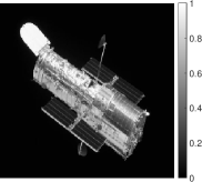
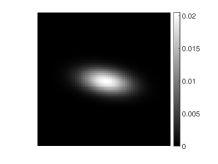
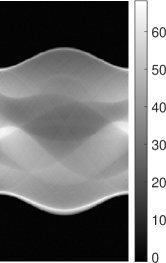
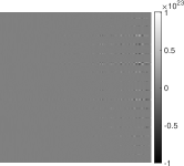
In Fig. 1 we display the test data that will be used through this paper, and that can be generated running the MATLAB script generate_blur.
 |
 |
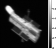 |
| (a) true image | (b) PSF | (c) observed image |
The size of the images are pixels, so . The matrix models a spatially invariant blur, with an anisotropic Gaussian PSF (whose analytical expression is given in [124, Chapter 3]) and reflective (sometimes referred to as reflexive) boundary conditions.
Tomographic reconstruction (or computed tomography, CT) is a critical tool in many applications such as nondestructive evaluation and electron microscopy; the advent of newer technologies (e.g., spectral CT and photoacoustic tomography) prompts more efficient and more accurate reconstruction methods. CT consists in computing reconstructions of (parameters of) objects from projections, i.e., data obtained by integrations along rays (typically straight lines) that penetrate a domain. More precisely, in a (semi)continuous setting, the unknown parameters are modeled as a function , , and it is assumed that the damping of a infinitesimally small portion of length of a ray penetrating the object at position is proportional to the product . The th observation , , is the damping of a signal that penetrates the object along the th ray (parameterized by a ray length ), and can be represented by the integral
| (3) |
where is a random perturbation corrupting the measurement. Employing a classical discretization scheme, which subdivides the object into an array of pixels and assumes that the function is constant in each pixel, the above integral can be expressed as a discrete sum and the following expression for the th entry of the sparse matrix can be readily derived as
where is the set of indices of those pixels that are penetrated by the th ray, is the length of the th ray through the th pixel. Thus, the basic CT problem Eq. 3 is of the form Eq. 1, where represents the unknown material parameters, represents a physical attenuation (damping) process, and contains the vectorized projections (as measured by a detector) and is often referred to as a sinogram. In most cases of tomography, is a rectangular matrix, where if fewer measurements are collected than the number of unknowns, or if many projections can be obtained, or parameterization reduces the number of unknowns. We refer to [31] for more details on the tomography reconstruction problem.
 |
|
 |
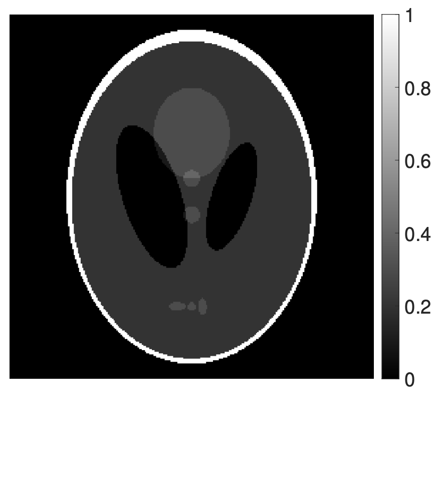
| (a) true image | (b) tomography setup | (c) observations |
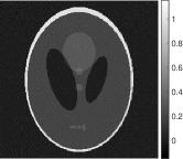
In Fig. 2 we display the test data for tomography that will be used through this paper, and that can be generated running the MATLAB script generate_tomo: this program still draws on IR Tools, which itself calls functions available within the MATLAB package AIR Tools II [122]. The object we wish to recover is the Shepp-Logan ‘medical’ phantom of size pixels, so that . The damping matrix is modeled after a parallel tomography process, where parallel rays are generated from a source ideally placed infinitely far from a flat detector; moreover, the source-detector pair is rotated around the object, and measurements are recorded for angles. Hence the number of observations is . One can vary the parameters that define the measurement geometry, such as the number of angles or the number of rays. For this example, we take measurements from to degrees in intervals of degree, resulting in a set of data with measurements, so that .
Now that we have addressed what is an inverse problem and looked at some examples of inverse problems, our focus turns to computing solutions to inverse problems, and for this we need regularization.
1.2 What is regularization and why do we need it?
Solving inverse problems is notoriously difficult due to ill-posedness222Here we consider the discretized problem, but point the reader to [70, 118] for discussions on the full implications of ill-posedness in continuous formulations., whereby data acquisition noise and computational errors can lead to large changes in the computed solution. For instance, if is invertible, the solution is dominated by noise and is useless for all practical purposes. The same happens for a more general and for the solution expressed as
| (4) |
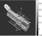
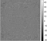
where is the generalized inverse of ; see [101]. We illustrate this phenomenon for the described test problems, where a tiny amount of noise (here, ) enters the data collection process. Naive inverse solutions for the image deblurring and tomography test problems are displayed in the first and third frames of Fig. 3, respectively. It is clear that these solutions are unacceptable approximations to (so much that, for image deblurring, the available corrupted image even looks better!).
| deblurring example | tomography example | ||
 |
 |
 |
 |
| inverse solution | regularized solution | inverse solution | regularized solution |
Regularization can be used to overcome the inherent instability of ill-posed problems in order to compute a meaningful solution. The basic idea of regularization is to replace problem Eq. 1 by a modified problem that incorporates other information about the solution. If proper regularization is applied, a regularized solution (e.g., the ones shown in the second and fourth frame of Fig. 3) should be close to the true solution. Regularization techniques come in many forms, and more details will be unfolded in the coming sections. However, for now, we consider two types of methods: variational regularization methods and iterative regularization methods.
Variational regularization methods for Eq. 1 involve solving optimization problems of the form,
| (5) |
where is a loss (or fit-to-data) function, is a regularization operator333Commonly-used regularization operators are based on smoothness constraints or assumptions of Gaussian priors., is a regularization parameter that controls the amount of regularization, thereby determining how faithful the modified problem is to the original problem, and denotes the set of feasible solutions (e.g., those that satisfy some constraints). The main advantage of formulation Eq. 5 is that general constraints and priors can be easily incorporated in the problem. Furthermore, well-known optimization methods can be used to solve Eq. 5. For the particular case where , direct factorization methods can, in principle, be used to compute a solution (see Section 2.1), although this is often computationally infeasible for large-scale problems. In this setting, the main disadvantage is the need to select the regularization parameter , often prior to solution computation.
On the other hand, iterative regularization methods for Eq. 1 typically consist in applying an iterative solver to
| (6) |
and computing a regularized solution by early termination of the iterations. In practice, when is expressed in the 2-norm, the iterative methods of choice are often subspace projection methods, whereby the problem is projected onto increasing (but relatively small) subspaces, and a projected subproblem is solved at each iteration by imposing certain optimality conditions on the approximated solution. Although an explicit choice of the regularization parameter is no longer required (contrary to Eq. 5), the stopping iteration essentially serves as a regularization parameter, as it balances how ‘faithful’ the projected problem is to the original problem. In this setting, the main disadvantage is that general constraints cannot be easily incorporated, and, even when they can, they can only be handled through complicated nested iterative schemes.
Hybrid regularization methods combine variational and iterative regularization methods, leveraging the best features of each class, to provide a powerful computational framework for solving large-scale inverse problems. In this paper, we focus specifically on hybrid projection methods that start off as iterative regularization methods, i.e., the original problem Eq. 1 is projected onto a subspace of increasing dimension, and then the projected subproblem is solved using a variational regularization method.
1.3 Why should we use hybrid projection methods?
The main motivations for using hybrid projection methods to solve large inverse problems can be grouped as follows.
-
•
For many multidimensional inverse problems (such as the model ones described in Section 1.1), the matrix is very large (to the point that it cannot be explicitly stored). In this setting, only matrix-vector multiplications with (and possibly ) can be performed, most often taking advantage of high-performance computing or tools such as GPUs. Therefore, methods that work explicitly with (e.g., methods that require some factorizations of , such as the singular value decomposition) are ruled out. Hybrid regularization methods can be implemented without explicitly constructing and storing the matrix , by treating and as linear operators.
-
•
Even when adopting a variational regularization method Eq. 5, one may not know a good regularization parameter in advance, and standard methods to estimate can be expensive: indeed, these typically require first approximating problem Eq. 1, or solving many instances of Eq. 1 with different regularization parameters. Hybrid projection methods provide a natural setting to estimate an appropriate value of during the solution computation process: often in a heuristic way, but in some cases with theoretical guarantees.
-
•
As mentioned above, many iterative solvers for Eq. 6, such as projection methods onto Krylov subspaces, have inherent regularizing properties and avoid data overfitting by early termination of the iterations. By using hybrid methods, it is possible to stabilize and enhance the regularized solutions computed by these methods. Moreover, hybrid methods enjoy nice theoretical properties. For instance we know that, for many hybrid frameworks, iterates obtained by first projecting the problem and then regularizing are mathematically equivalent to iterates obtained by first regularizing and then projecting the regularized problem.
-
•
Hybrid methods provide a convenient framework for the development of extensions to more general problems and regularization terms. For instance, one could incorporate a variety of regularization terms of the form , where , or also consider functions that are not expressed in the 2-norm. As we will see in Section 4, this amounts to modifying the projection subspace that can be used within hybrid methods. By doing so, other popular (but expensive) iterative regularization schemes (which are often based on nested cycles of iterations) can be avoided.
1.4 Outline of the paper
The remaining part of this survey is organized as follows. In Section 2, we describe the general problem setup to provide some background for hybrid methods, including an overview of the most relevant direct and iterative regularization techniques. Then, in Section 3, we discuss hybrid projection methods. After providing a brief summary of the historical developments of hybrid methods, we address the two main building blocks of any hybrid method: namely, generating a subspace for the solution (Section 3.2.1) and solving the projected problem (Section 3.2.2). Important numerical and theoretical aspects will also be covered: these include strategies to efficiently set the Tikhonov regularization parameter and stop the iterations (Section 3.3) and available convergence proofs and approximation properties (Section 3.4). In recent years, we have witnessed the extension of hybrid methods to solve a larger scope of problems and to cover broader scientific applications. In Section 4, we provide an overview of some of these extensions:
-
•
Beyond standard-form Tikhonov: Hybrid projection methods for general-form Tikhonov; see Section 4.1
-
•
Beyond standard projection subspaces: Enrichment, augmentation, and recycling; see Section 4.2
-
•
Beyond the 2-norm: Sparsity-enforcing hybrid projection methods for regularization; see Section 4.3
-
•
Beyond deterministic inversion: Hybrid projection methods in a Bayesian setting; see Section 4.4
-
•
Beyond linear forward models: Hybrid projection methods for nonlinear inverse problems; see Section 4.5
Pointers to relevant software packages are provided in Section 5. Conclusions and outlook on future directions are provided in Section 6.
Notations
Boldface lower-case letters denote vectors: e.g., ; , denotes the th component of the vector . Boldface upper-case letters denote matrices: e.g., ; , , , denotes the th entry of the matrix . Indexed matching boldface lower-case letters denote matrix columns: e.g., , denotes the th column of the matrix . denotes the identity matrix of size , whose columns , are the canonical basis vectors of . The column space of a matrix is denoted by . Lower-case Greek letters, sometimes indexed, are often used to denote scalars. In the following, when there is no ambiguity (essentially until Section 4), the shorthand notation will be used.
2 General problem setup and background
For the simplified case where , , and in Eq. 5, we get the so-called standard-form Tikhonov problem,
| (7) |
We stress that the standard-form Tikhonov problem has been widely studied in both the mathematics and statistics communities and has been used in many scientific applications. However, computing Tikhonov-regularized solutions can still be challenging if the size of is very large or if is not known a priori. In fact, being able to efficiently compute solutions to Eq. 7 was a main motivation for much of the early works on hybrid projection methods. For a discussion on extensions of hybrid methods to solve more general problems including the general-form Tikhonov problem, see Section 4.
2.1 SVD-based direct regularization methods
In this section, we begin with the standard-form Tikhonov problem Eq. 7, and describe a direct approach based on the singular value decomposition (SVD) of to compute a solution. For the problems of interest, direct application of this approach is not computationally feasible. However, the formulations briefly explored here will be useful for analysis and interpretation later in this paper. Furthermore, in the hybrid framework, the direct methods described here can be used to solve the projected problem. We point the interested reader to [118] for a more thorough exposition of direct methods.
Without loss of generality, let us assume that with . The SVD of is defined as
| (8) |
where and are orthogonal and contains the singular values, .
The solution to Eq. 7 can be written as
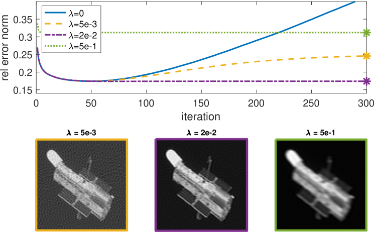
are the Tikhonov filter factors. Tikhonov regularization is one example from a wider class of spectral filtering methods. SVD-filtering methods compute regularized solutions by imposing suitable filtering on the SVD components of the solution: namely, the filter factors should be close to for small , and should approach for large . The Tikhonov filter factors have this property, with the amount of filtering prescribed by the regularization parameter . Indeed, for small values of , little weight is put on the regularization term and the filter factors are more prone to approach (or, at least, a good portion of filter factors are close to , depending on the location of within the range of the singular values of ). Thus, regularized solutions may be ‘under-regularized’, i.e., still contaminated with noise. However, for large values of , too much weight is put on the regularization term and the filter factors are more prone to approach , so solutions may be ‘over-regularized’ or ‘over-smoothed’. We refer the reader to the images provided in Fig. 5 for an illustration of the impact of the regularization parameter on the solution.
Also the truncated SVD (TSVD) method, which regularizes Eq. 1 by computing
is a filtering method, with filter factors obtained by first setting a truncation index , and by then considering , if , and otherwise. Note that choosing returns the unregularized solution of Eq. 1. Therefore, plays the role of regularization parameter.
Every spectral filtering method requires the selection of a regularization parameter. Common strategies to do so include the discrepancy principle [155], the generalized cross-validation (GCV) method [95], the unbiased predictive risk estimation (UPRE) method [207], and the -curve [150]. Since there is not one method that will work for all problems, it is usually a good idea to try a variety of methods. For problems where the SVD of is available, one can efficiently apply these regularization parameter strategies. For problems where computing the SVD is not feasible, parameter choice strategies are limited. However, we will see in Section 3.3 that many of these existing regularization parameter selection techniques are not only feasible but also can be successfully integrated within hybrid projection methods.
The SVD of Eq. 8, besides being an essential building block of SVD-filtering methods, is a pivotal tool for the analysis of discrete inverse problems [70, 117, 118]. For instance, looking at the decay of the singular values, one may infer different degrees of ill-posedness: typically, following [130], a polynomial decay of the form , , is classified as mild (if ) or moderate (if ) ill-posedness, while an exponential decay of the form , , is classified as severe ill-posedness. The Picard condition, which in the continuous setting provides necessary and sufficient conditions for the existence of a solution of the form Eq. 4 [70], can be adopted in a discrete setting to gain insight into the relative behavior of the magnitude of and , which appear in the expression of the (filtered) solutions. Employing tools such as the so-called ‘Picard plot’ [118] can inform us on the existence of a meaningful solution to Eq. 1 as well as the effectiveness of any (filtering) regularization method applied to Eq. 1.
2.2 Iterative regularization methods
Next we describe iterative regularization, where an iterative method is used to approximate the solution of the unregularized least-squares problem,
| (9) |
and early termination of the iterative process results in a regularized solution. We focus on projection methods where the underlying concept is to constrain the solution at the th iteration to lie in a -dimensional subspace spanned by the (typically orthonormal) columns of some matrix , where . That is, the regularized solution is given as
| (10) |
We are interested in projection methods using Krylov subspaces [187]. Given and , a Krylov subspace is defined as
Here and in the following, we assume that the dimension of is . When Krylov methods are employed to solve problem Eq. 9, and are defined in terms of and , respectively. In iterative regularization methods based on the Arnoldi process (such as GMRES), the columns of form an orthonormal basis for , where must be square. However, for problems where is not square (e.g. in tomography), iterative regularization methods based on the Lanczos or Golub-Kahan bidiagonalization process (such as LSQR [170, 169] or LSMR [75]) are used, and the columns of form an orthonormal basis for . Note that LSQR is mathematically equivalent to CGLS, i.e., the conjugate gradient (CG) method applied to the normal equations. All the Krylov methods mentioned so far are minimum residual methods, so that the th iterate can be written as , where solves Eq. 10. More details regarding the generation of these basis vectors will be addressed in Section 3.2.1.
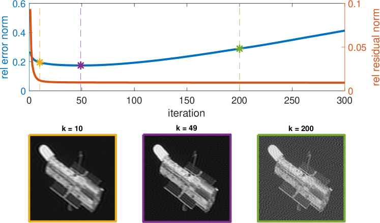
A crucial feature of classical Krylov methods when applied to ill-posed inverse problems is that, oftentimes, these iterative methods exhibit a regularizing effect in that the projection subspace in early iterations provides a good basis for the solution. One of the first Krylov methods that was proven to have regularizing properties is CGLS [160, 112]. Indeed, the CGLS iterates can be expressed as filtered SVD solutions [118]. Since these iterative methods converge to the least-squares solution, we get a phenomenon commonly referred to as ‘semi-convergence’ (after [159]), whereby the relative reconstruction errors decrease at early iterations but increase at later iterations due to noise manifestation and amplification. See Fig. 4 for an illustration. Because of this, for iterative regularization, the stopping iteration plays the role of the regularization parameter. There have been many investigations into developing stopping criteria for iterative methods for inverse problems. If a good estimate of the amount of noise is available, the most widely used and intuitive approach is to stop iterating as soon as the value of the objective function in Eq. 10 reaches the magnitude of the noise: this is the so-called discrepancy principle. GCV and modifications of GCV have also been used for stopping criteria [19, 21, 55]. We again refer to Section 3.3 for more details about these strategies. The main challenge is that for some problems, the reconstruction can be very sensitive to the choice of the stopping iteration. Thus, if the method stops a little too late, the reconstruction is already contaminated by noise (i.e., under-regularized). On the contrary, if the iterations are stopped too early (i.e., over-regularization), a potentially better reconstruction is precluded. We remark that it has been observed that semi-convergence may appear somewhat ‘prematurely’ and that it is sometimes important to have a larger approximation subspace (which would otherwise be beneficial for the solution; see [132, 167]).
In some circumstances, even if direct regularization methods are feasible, one may prefer to adopt iterative regularization methods. Some reasons are highlighted in [113], where the following heuristic motivation is given: contrary to TSVD, Krylov methods (such as LSQR) generate an approximation subspace that is tailored to the current right-hand-side vector. Therefore, the basis vectors for the solution may be better ‘adapted’ to the given problem than the right singular vectors.
In many fields from numerical linear algebra to differential equations, iterative methods and, in particular, preconditioned Krylov methods, have been immensely successful in solving large, sparse systems of equations efficiently [187]. Iterative methods have also gained widespread use in the inverse problems community. One of the main reasons for this is that neither the matrix nor its factorization need to be constructed, and thus, these methods are ideal for large-scale problems. Furthermore, it has been observed many times that the generated Krylov subspaces are rich in information for representing the solution (i.e., corresponding to the large singular vectors). Thus, a reasonable solution can be obtained in only a few iterations. The greatest caveat for inverse problems is semi-convergence, so great care must be taken to find good stopping criteria. In Section 3.4 we will dwell more on the properties of the approximation subspaces generated by different projection methods.
2.3 Iterative methods for solving the Tikhonov problem
As described in Section 2.1, the Tikhonov problem Eq. 7 can be easily solved if the SVD of is available and, in this case, many well-regarded parameter choice strategies can be applied to compute a suitable value of the regularization parameter . Nonetheless, for large-scale problems where cannot be constructed but matrix-vector products with and can be computed efficiently, iterative projection methods [170, 169] can be used to solve the equivalent Tikhonov problem,
| (11) |
However, this approach may not be convenient if a suitable value of is not known a priori. In this case, often one must solve problem Eq. 11 from scratch for many different values of and this eventually results in an expensive approach (note that for specific iterative solvers, one may adopt smart strategies to reduce computations; see [78]).
Similar to the discussion in Section 2.1, the value of can have a considerable impact on the quality of the reconstructed solution. Moreover, when using iterative methods to solve the Tikhonov problem, one can to some extent leverage the number of iterations to enforce additional regularization. For illustration, we use CGLS to solve Eq. 11 for various choices of for the image deblurring example and provide relative reconstruction error norms per iteration in Fig. 5. Notice that if is chosen too small, severe semi-convergence appears and a good stopping iteration is as crucial as for the ‘purely’ iterative (i.e., ) methods introduced in Section 2.2; on the contrary, if is chosen too large, the solution is over-regularized and additional iterations cannot mitigate this phenomenon. Thus, seems to have a greater impact on the quality of the reconstructed solution than the number of iterations, which can be attributed to the modification of the spectral properties of the coefficient matrix in Eq. 11.
We can draw the following conclusions about the successful working of a standard iterative method to solve a Tikhonov regularized problem. First, the user must be reasonably confident in the choice of the regularization parameter. Second, the user must be cognizant about the interplay of the choice of the regularization parameter and the number of iterations for Eq. 11, as both of these contribute to a suitable regularized solution. As we will see in the next section, hybrid projection methods provide an alternative approach of combining an iterative method and Tikhonov regularization, whereby a regularization parameter can be automatically and adaptively tuned during the iterative process.
3 Hybrid projection methods
A hybrid projection method is an iterative strategy that regularizes problem Eq. 9 by projecting it onto subspaces of increasing dimension and by solving the projected problem using a variational regularization method. Formally, recalling the framework for iterative projection methods unfolded in Eq. 10, the solution at the th iteration of a hybrid projection method for standard Tikhonov can be represented as
| (12) |
Notice that the solution incorporates both regularization from the projection subspace (determined by the choice of the projection method, i.e., and ) and a potentially changing variational regularization term (defined by ). Again, for simplicity and for historical reasons, in this section we focus on the standard-form Tikhonov problem Eq. 7; extensions will be considered in Section 4.
An illustration
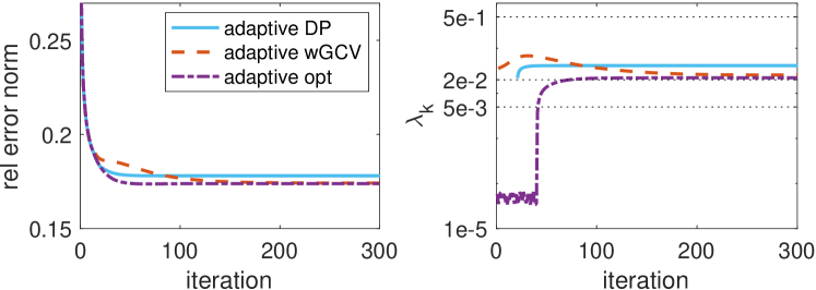
Before we get into the details of hybrid projection methods, we begin by illustrating the benefits of allowing adaptive choices for the regularization parameter, where a different regularization parameter can be used at each iteration, i.e., . In Fig. 6 for the image deblurring problem, we provide relative reconstruction error norms per iteration in the left panel and computed regularization parameters per iteration in the right panel. Here, ‘opt’ refers to selecting at each iteration the regularization parameter that delivers the smallest relative reconstruction error. Parameter selection methods ‘DP’ and ‘wGCV’ and others will be discussed in Section 3.3. Notice that relative reconstruction errors using (appropriately selected) adaptive regularization parameters can overcome semi-convergence behavior (see Fig. 4) and result in reconstruction errors that are close to a pre-selected optimal regularization parameter. For early iterations, a small (corresponding to little variational regularization) is sufficient, but as iterations progress, the adaptive methods should select regularization parameters close to the optimal one.
An algorithm
Now that we have seen the potential benefits of a hybrid projection method, let us discuss the general structure of such algorithms. A sketch of a hybrid projection method for standard Tikhonov regularization is provided in Algorithm 3.1, with links to the appropriate sections of the paper for more details. Notice that each iteration requires the expansion of the projection subspace and the solution of a projected regularized problem where a regularization parameter can be selected at each iteration.
An outline of the remaining part of this section is as follows. We begin in Section 3.1 with a brief historical overview of hybrid projection methods. Details and derivations for hybrid projection methods can be found in Section 3.2, where we describe some techniques for steps 2 and 4 of Algorithm 3.1: namely, expanding the projection subspace (e.g., via the Arnoldi or Golub-Kahan process) and solving the projected regularized problem. One of the main advantages and features of a hybrid projection method is the ability to select regularization parameters automatically and adaptively (i.e., during the iterative process as in step 3 of Algorithm 3.1). Thus, we dedicate Section 3.3 to providing an overview of regularization parameter selection methods, with a particular emphasis on methods that have been critical for the success of hybrid projection methods. Although we still do not have a complete analysis of the regularizing properties of every hybrid projection method, important theoretical results and properties have nonetheless been established for specific methods, and we highlight some of these in Section 3.4.
3.1 Historical development of hybrid methods
Since the seminal publication by O’Leary and Simmons in 1981 [167], there have been four decades of progress and developments in the field of hybrid projection methods. A quick google scholar search shows that the number of citations for this paper alone nearly doubles in each subsequent decade. In this section, we provide a brief overview of the main contributions and highlights by decade. This is by no means an exhaustive list of publications, and we realize that there may be bias in the selections, but our goal is to provide the reader with some historical context. For a novice reader, this section can be skipped upon first reading.
1981-1990
To the best of our knowledge, the first journal publication to introduce a hybrid projection method was by O’Leary and Simmons in 1981 [167], in which they describe a ‘projection-regularization’ method that combines the Golub-Kahan bidiagonalization for projection and TSVD for regularization. In the paper, the authors mention that a different hybrid algorithm was proposed independently, with a reference to a technical report by Björck in 1980 [18]. Björck’s work appeared in BIT in 1988 [19], where a key difference was that the right hand side vector was used as the starting vector, since it was noted that allowing the algorithms to start with an arbitrary vector did not always perform well. Other algorithmic contributions included the use of cross-validation to determine stopping criteria and transformations to standard form based on Eldén’s earlier work [68]. Example problems from time series deconvolution were used in [167], but the computational technology at the time was still quite limited [195].
1991-2000
During this period, hybrid projection methods gained significant traction in the numerical linear algebra community as well as practical utility in various seismic imaging applications [217, 188]. As described in Björck’s book [20], various researchers were interested in characterizing the regularizing properties of Krylov methods (e.g., see Nemirovskii [160] and various works by Hanke and Hansen [114]), where the main motivation was to determine appropriate stopping criteria for iterative methods when applied to ill-posed problems. Advancements in hybrid methods included investigations into stable computations (e.g., reorthogonalization) by Björck, Grimme and Van Dooren [21] as well as new methods for selecting regularization parameters. For example, Calvetti, Golub and Reichel [33] proposed a hybrid approach where a so-called ‘-ribbon’ was computed using a partial Lanczos bidiagonalization. The first application of hybrid methods for large, nonlinear inversion was described in Haber and Oldenburg [109], and hybrid approaches based on projections with GMRES or Arnoldi were described by Calvetti, Morigi, Reichel, and Sgallari in [40]. In terms of software, Hansen laid some groundwork for hybrid methods in the Regularization Tools package [116], where routines for computing the lower bidiagonal matrix and the SVD of a bidiagonal matrix were provided.
Not all of the work on hybridized methods during this time followed the project-then-regularize framework. Related work on estimating the regularization parameter for large-scale Tikhonov problems by exploiting relationships with CG also appeared during this time. For example, Golub and Von Matt [103] estimated the GCV parameter for large problems using relations between Gaussian quadrature rules and Golub-Kahan bidiagonalization, and Frommer and Maass [78] exploited the shift structure of CG methods to solve Tikhonov problems with multiple regularization parameters simultaneously.
2001-2010
With significant improvements in computational resources and capabilities, researchers became interested in how to realize the benefits of hybrid projection methods in practice. In this decade, we saw a surge in the development of regularization parameter selection methods for hybrid projection methods [145, 34, 55, 153, 209] and various extensions of hybrid methods to include general regularization terms (e.g., total variation [38] and general-form Tikhonov [144, 128]). Still, the main focus was on TSVD and Tikhonov for regularization. New interpretations of hybrid methods based on Lanczos and TSVD were described in [113], and noise level estimation from the Golub-Kahan bidiagonalization process, which can be used for determining the stopping iteration, were described in [127]. A fully automatic MATLAB routine called ‘HyBR’ was provided in [55], where a Golub-Kahan hybrid projection method with a weighted GCV parameter choice rule was implemented for standard Tikhonov regularization. Hybrid methods were implemented on distributed computing architectures [59] and were used for many new applications such as cryoelectron microscopy and electrocardiography [140].
2011-present
At present, hybrid projection methods have gained significant interest in many research fields, and contributions range from new methodologies and advanced theories to innovations in scientific applications. Many of the recent developments in hybrid methods will be elaborated on in Section 4, so here we just provide some highlights. In particular, there have been many papers on the Arnoldi-Tikhonov method [88, 90]. Flexible and generalized hybrid methods based on state-of-the-art Krylov subspace methods have been introduced for including more general regularization terms and constraints [147, 175, 85, 57, 51, 81]. There have been connections made to the field of computational uncertainty quantification [191] and new insights in the regularization parameter selection strategies [181], and regularization by approximate matrix functions [24, 60, 165]. There exists a plethora of papers in application and imaging journals, and a new software package called IR Tools [79]. We also refer interested readers to an older survey paper on Krylov projection methods and Tikhonov regularization [91].
3.2 Algorithmic approaches to hybrid projection methods
Following derivations of iterative methods for sparse rectangular systems, in Section 3.2.1 we first describe common techniques to iteratively build a solution subspace and to efficiently project problem Eq. 9 onto subspaces of increasing dimension. Then, in Section 3.2.2, we describe techniques to solve the projected regularized problem.
3.2.1 Projecting onto subspaces of increasing dimension
In this section, we address the first building block of a hybrid projection method, which is to use an iterative method to build a sequence of solution subspaces of small but increasing dimension, and to efficiently project the problem onto them. The first important question to address is: in practice, what makes a good solution subspace? Indeed, a clever choice of basis vectors should satisfy multiple requirements. Since the number of iterations required for solution computation should be small, a good basis should be able to accurately capture the important information in a few vectors. In this sense, the SVD basis vectors (i.e, the columns of in Eq. 8) would be ideal (recall discussion about filtered SVD in Section 2.1). Unfortunately, computing the SVD can be infeasible for very large problems. Thus, we seek a subspace sequence that exhibits a rapid enough decrease in the residual norm in Eq. 9 so that early termination provides good approximations [101]. Another desirable property is that the solution subspace can be generated efficiently. Here we mean that the main computational cost per iteration is manageable, i.e, requires one matrix-vector multiplication with and possibly one with . Lastly, for numerical stability it may be desirable to have an orthogonal basis for the solution subspace [166]. Although a variety of projection methods and solution subspaces could be used, here we focus on two of the most common projection methods on Krylov subspaces, namely the Arnoldi process and the Golub-Kahan bidiagonalization process. We will argue that these algorithms compute good solution spaces, according to the criteria listed above.
Arnoldi process
The Arnoldi process generates an orthonormal basis for at the th iteration [187]. Given matrix and vector with initialization where , the th iteration of the Arnoldi process generates vector and scalars for such that, in matrix form, the following Arnoldi relationship holds,
| (13) |
where
and where, in exact arithmetic, Notice that contains an orthonormal basis for and is an upper Hessenberg matrix (i.e., upper triangular with the first lower diagonal). The Arnoldi process is summarized in Algorithm 3.2.
Notice that the main computational cost of each iteration of the Arnoldi process is one matrix-vector multiplication with . Breakdown of the iterative process may happen (when ), but we are typically not concerned about this because these methods are meaningful only when the number of iterations is not too high.
One caveat, especially for inverse problems such as tomography, is that the Arnoldi method relies on the fact that is square. For rectangular problems, one could apply the Arnoldi process to the normal equations , in which case the Arnoldi algorithm simplifies to the symmetric Lanczos tridiagonalization process where, thanks to symmetry, is tridiagonal rather than upper Hessenberg. However, a numerically favorable approach would be to avoid the normal equations and to work directly with and separately. This is achieved by adopting the Golub-Kahan bidiagonalization process, which we describe next; we will also state more precisely the links between the Golub-Kahan bidiagonalization and the symmetric Lanczos process.
Golub-Kahan bidiagonalization process
Contrary to the Arnoldi process that generates only one orthonormal basis (i.e, for ), the Golub-Kahan bidiagonalization (GKB) process generates two sets of orthonormal vectors that span Krylov subspaces and [96]. Given a matrix and a vector with initialization where and where , at the th iteration of the GKB process, we generate vectors , , and scalars and such that in matrix form, the following relationships hold,
| (14) |
where
is bidiagonal, and . In exact arithmetic has orthonormal columns that span and has orthonormal columns that span . The GKB process is summarized in Algorithm 3.3.
The main computational cost of each iteration of the GKB process is one matrix-vector multiplication with and one with . Breakdown in the GKB algorithm would occur when or but, similarly to the Arnoldi process, we will assume that breakdowns do not happen. A potential concern with the GKB process is loss of orthogonality in the vectors of and , for which it may be necessary to use a reorthogonalization strategy to preserve convergence of the singular values. Indeed, it has been shown that reorthogonalization of only one set of vectors is necessary [196, 12]; more details are provided in Section 3.4.
As mentioned above, GKB Eq. 14 is related to the symmetric Lanczos decomposition. Notice that, multiplying the first equation in Eq. 14 from the left by , and using the second equation in Eq. 14, we obtain
The above chain of equalities is the symmetric Lanczos algorithm applied to and , generating an orthonormal basis for . Similarly, multiplying the second equation in Eq. 14 (written in terms of ) on the left by , and using the first equation in Eq. 14, we obtain
| (15) |
The above chain of equalities is the symmetric Lanczos algorithm applied to and , generating an orthonormal basis for .
Comparison of Solution Subspaces
Although the choice of a projection method relies heavily on the problem being solved, there have been some investigations into which projection methods might be better suited for certain types of problems, especially in light of some recent work on flexible methods, general-form Tikhonov regularization, and matrix transpose approximation. We remark that the discussion here also relates to the material in Section 3.4.
For Arnoldi based methods, which build the approximation subspace starting from , a potential concern is the explicit presence of the (rescaled) noise vector among the basis vectors [135]. For problems with very low noise level, this is not a significant drawback [37]. However, various methods have been developed to remedy this. For example, the symmetric range-restricted minimum residual method MR-II [111] and the range-restricted GMRES (RRGMRES) method [36] discard and seek solutions in the Krylov subspace . For various projection methods, Hansen and Jensen [121] studied the propagation of noise in both the solution subspace and the reconstruction, noting the manifestation of band-pass filtered white noise as ‘freckles’ in the reconstructions.
For both the Arnoldi and the GKB process, notice that each additional vector in the Krylov solution subspace is generated by matrix-vector multiplication with or respectively. Therefore the vectors defining the Krylov solution space are iteration vectors of the power method for computing the largest eigenpair of a matrix, and hence they become increasingly richer in the direction of the dominant eigenvector of or . For many inverse problems (and due to the discrete Picard condition), the orthonormal basis solution vectors generated in early iterations tend to carry important information about the low-frequency components (i.e., the right singular vectors that correspond to the large singular values) [118]. Therefore, the Krylov subspaces considered in this section can be appropriate choices for use in hybrid projection methods.
It is important to note that the choice of Krylov subspace may be problem dependent. For some image deblurring problems, it has been observed that Arnoldi-based methods may not be suitable since multiplication with corresponds to recursive blurring of the observation, resulting in a poor solution subspace. Various modifications have been proposed. For example, for image deblurring problems with nonsymmetric blurs and anti-reflective boundary conditions, ‘preconditioners’ were used to improve the quality of the computed solution when using Arnoldi-Tikhonov methods [65]. For tomography applications where the coefficient matrix is often rectangular, it is natural to consider Golub-Kahan based methods; even if the matrix modeling a tomographic acquisition problem happens to be square (because of a specific scanning geometry), it should be stressed that standard Arnoldi methods would not generate a meaningful approximation subspace for the solution. This is because multiplication with maps images to sinograms, and subsequent mappings to sinograms are neither physically meaningful nor fit for image reconstruction. Nonetheless, a specific ‘preconditioned’ GMRES method, with ‘preconditioners’ modeled as backprojection operators, has been used for tomography in [61].
It should be noted that preconditioning ill-posed problems can be a tricky business [115]. Indeed, besides improving the solution subspace, preconditioning can also be cautiously used with the classical goal of accelerating convergence (provided that it does not exacerbate the semi-convergence phenomenon). Flexible (right) preconditioners have also been considered as means to improve the solution subspace [85, 51]. Sometimes additional vectors (that are hopefully meaningful to recover known features of the solution) can be added to the approximation subspace, where the goal is not necessarily to accelerate convergence, but rather to improve the solution subspace. This is the idea behind the so-called enriched or recycling methods (see, for instance, [66, 119]); these are described in more detail in Section 4.2.
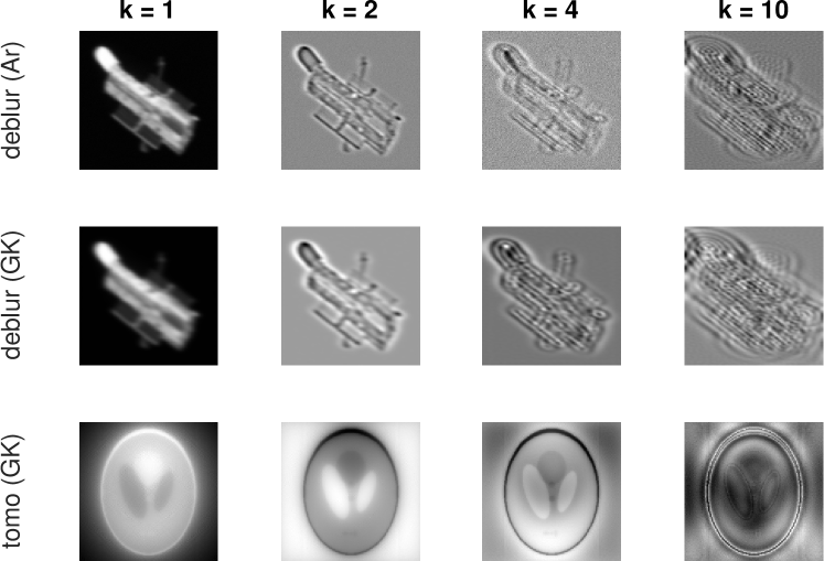
In Fig. 7, we show a few of the basis vectors for the solution generated by the Arnoldi and the GKB algorithms applied to the image deblurring and the tomography reconstruction problems described in Section 1. The displayed images are reshaped columns of . For the deblurring example, we observe that, as expected, the first basis vector for the GKB process (i.e., ) is smoother or more blurred than that from the Arnoldi process (i.e., ). However, we notice that the th basis vector computed by Arnoldi may have more details but is more noisy than that for GKB. For the tomography example, we provide some of the GKB solution basis vectors, for which we note that the basis vector for the first iteration is the scaled vector , which can be interpreted as an unfiltered backprojection image; see [159].
3.2.2 Solving the regularized, projected problem
In Section 3.2.1, we described two iterative projection methods that can be used to generate and expand the projection subspace (step 2 in Algorithm 3.1). Although projection onto subspaces of increasing dimension (e.g., Krylov subspaces) can have an inherent regularizing effect (recall the discussion in Section 2.2), a key component of hybrid projection methods is the combination of iterative and variational regularization, i.e., the inclusion of a regularization term within the projected problem. We remark that Steps 3 and 4 in Algorithm 3.1 are closely intertwined and could easily be addressed together. However, for clarity of presentation, methods to select the regularization parameter and the stopping iteration will be addressed in detail in Section 3.3, and this section will focus on solving the projected regularized problem Eq. 12. Notice that at step 4 of Algorithm 3.1, we have computed and , and the stopping criterion is not yet satisfied.
Computing a solution to Eq. 12 can be done efficiently by exploiting components and relationships from the projection process (Eq. 13 for Arnoldi and Eq. 14 for GKB). In this section, we denote the solution subspaces for Arnoldi and Golub-Kahan as and respectively.
The hybrid GMRES iterate at the th iteration is given by
| (16) | ||||
Note that, since if , we can equivalently write
Oftentimes, the hybrid GMRES approach is referred to as an Arnoldi-Tikhonov approach [37, 151, 91].
Similar derivations can be done for the Golub-Kahan projection method. In particular, the hybrid LSQR iterate is computed as
| (17) |
or, equivalently,
The hybrid LSMR iterate [56] is computed as
| (18) |
where
Table 1 provides a summary of common methods with their defining subspace and corresponding subproblem.
| method | subspace | subproblem |
|---|---|---|
| hybrid GMRES | Arnoldi, | |
| hybrid LSQR | Golub-Kahan, | |
| hybrid LSMR | Golub-Kahan, |
One important property to highlight is that, for these methods, the generated subspace is independent of the choice of the regularization parameters. This is not always true (e.g., in the flexible methods presented in Section 4.3). A very desirable consequence of this is that one can avoid computing the regularized solution at each iteration. For many of the regularization parameter selection methods, the choice of the parameter at each iteration does not depend on previous or later iterates. Thus, it is possible to delay regularization parameter selection and solution computation until a solution is needed or some stopping criterion is satisfied.
Next, we draw some connections and distinctions to standard iterative methods for least-squares problems (i.e., for the case where or , fixed along the iterations). For problems where no regularization is imposed on the projected problem (i.e., ), we recover standard iterative methods GMRES for Arnoldi (solving Eq. 16) and LSQR for GKB (solving Eq. 17).
For hybrid projection methods, a potential concern is the need to store all of the solution vectors . For Arnoldi based methods for solving Tikhonov regularized problems, this requirement is the same as for standard iterative methods. However, for Golub-Kahan based methods, this potential caveat warrants a discussion. Indeed, it is well-known that the LSQR iterates can be computed efficiently using a three-term-recurrence property by exploiting an efficient QR factorization of . As shown in [169], such computational efficiencies can also be exploited for standard Tikhonov regularization if is fixed a priori. This can be done by exploiting the fact that the Krylov subspace is shift invariant with respect to However, semi-convergence will be an issue if and the entire process must be restarted from scratch if a different is desired. This computational flaw is even more severe when using iterative methods such as LSQR for general-form Tikhonov regularization, since the solution subspace typically depends on the regularization parameter and the regularization matrix (although some strategies to ease this dependence are described in Section 4.1). For hybrid projection methods based on GKB, storage of the solution vectors is the main additional cost associated with the ability to select adaptively during the hybrid projection procedure. For problems that require many iterations, potential remedies include developing a good preconditioner, compression and/or augmentation techniques [139].
3.2.3 A unifying framework
All the methods described so far can be expressed by this partial factorization,
| (19) |
where the columns of are orthonormal and span the -dimensional approximation subspace for the solution, the columns of are orthonormal with and span a -dimensional subspace (e.g., associated to ), and is a matrix that has some structure and represents the projected problem. For hybrid GMRES, , and are given in (13). For hybrid LSQR and hybrid LSMR, , , and are given in (14). Let the SVD of the matrix be given by
| (20) |
where and are orthogonal, and contains the singular values of . Note that, for notational convenience, we have dropped the subscript .
For hybrid GMRES and hybrid LSQR with standard Tikhonov regularization, the solution to the regularized projected problems (16) and (17) have the form,
| (21) |
and thus one may express the th iterate of the hybrid projection method as
| (22) |
Note that by construction.
For many of the regularization parameter selection methods described in Section 3.3 and the theoretical results in Section 3.4, it will be helpful to define the so-called ‘influence matrix’,
| (23) |
For purely iterative methods (where ), the influence matrix is given by
Also, it will be helpful to define the so-called ‘discrepancy’ (or ‘regularized residual’) at the th iteration as
| (24) |
for hybrid methods; the same definition applies to iterative methods, with . In the following, we will adopt the notation and to denote the regularized inverse and the discrepancy associated to (direct) Tikhonov regularization, coherently to Eq. 22 and Eq. 24, respectively. When no regularization method is specified, , and denote a generic regularized solution, inverse, and residual, respectively.
3.3 Regularization parameter selection methods
The success of any regularization method depends on the choice of one (or more) regularization parameter(s). This was illustrated in Section 2 for Tikhonov regularization and for iterative regularization methods; also, when the Tikhonov-regularized problem is solved using an iterative method, both the Tikhonov regularization parameter and the number of iterations should be accurately tuned (see Section 2.3). Similarly, for hybrid projection methods, there are inherently two regularization parameters to tune: (1) the number of iterations (i.e., the dimension of the projection subspace), and (2) the regularization parameter for the projected problem (e.g., for Tikhonov). It is important to note that, when carelessly applied to hybrid projection methods where both regularization parameters must be determined, standard regularization parameter choice strategies seldom produce good results. Instead, a two-pronged approach is typically adopted, where a well-established parameter choice strategy is used to determine and one or more stopping rules are used to terminate the iterations, typically by monitoring the stabilization of some relevant quantities; see, for instance, [55, 88, 181, 33, 145]. Before describing specific parameter selection strategies, we comment on a few factors that are unique to selecting regularization parameters in a hybrid projection method, and that should be considered when determining which parameter selection methods to employ.
Selecting
Assume that is fixed and consider the case of standard form Tikhonov regularization. First, for many Krylov subspace projection methods, the projection subspace is independent of the current value of the Tikhonov regularization parameter. This is due to the shift-invariance property of the computed Krylov subspaces, and this has the effect that the approximate solution at the th iteration only depends on the current regularization parameter . Second, notice that, for a fixed , the projected problem (21) is a standard Tikhonov-regularized problem. A natural idea would be to directly apply well-established (e.g, SVD-based) parameter choice strategies that were developed for Tikhonov regularization; however, these methods are not self-contained in the hybrid setting, and care must be taken to ensure accurate results. Third, since the number of iterations is significantly smaller than the size of the original problem (i.e., ) and the projected problem has order (i.e., the coefficient matrix has size ), computations with can be performed efficiently. For many methods, there are computational advantages to using the SVD of Eq. 20. Indeed, the computational cost of obtaining (20) is negligible compared to the computational cost of performing matrix-vector products with (and possibly ) to expand the approximation subspace. We will see how some common parameter choice methods can be efficiently formulated using the SVD.
Selecting
Various rules have been developed for selecting the stopping iteration , and these rules can be employed quite generally (and independently of the parameter choice rule for ). The main idea is to terminate iterations when a maximum number of iterations is achieved or when one or more of the following conditions are satisfied:
| (25) |
where , , are positive user-specified thresholds. The rationale behind these approaches is that, often and broadly speaking, when stabilization happens, the selected value for the regularization parameter is suitable for the full-dimensional Tikhonov problem and the approximated solution cannot significantly improve with more iterations. Although this argument is mainly empirical, in some cases it is supported by theoretical results; see Section 3.3.4. This property is also heavily exploited in [102, 53, 180], where the regularization parameter (and other relevant quantities) for the original Tikhonov problem are estimated by projecting the original problem onto subspaces of smaller dimension. Once the regularization parameter is estimated, it is fixed and any iterative method can be used to solve the resulting Tikhonov problem; therefore, these methods are not considered hybrid projection methods as defined in this manuscript; see Section 1 and Section 2.3. The left frame of Fig. 6 displays the typical behavior of adaptively chosen regularization parameters where, relevant to the first criterion in Eq. 25, some stabilization is visible as the iterations proceed. Returning to the issue of selecting a stopping iteration for hybrid projection methods, we remark that, with a suitable choice of , hybrid methods can overcome semi-convergent behavior, as illustrated in Fig. 4. Thus, an imprecise (over-)estimate of the stopping iteration does not significantly degrade the reconstruction quality. In fact, one can typically afford a few more iterations without experiencing deterioration of the solution (on the contrary, the solution may improve because it is computed by solving a well-posed problem in a larger approximation subspace). This insight is also linked to the ability of the considered Krylov projection methods to ‘capture’ the dominant (i.e., relevant) truncated right singular vector subspace information to reconstruct the solution; we present more details about this in Section 3.4.
Parameter choice rules represent a large and growing body of literature in the field of inverse problems, with papers ranging from theoretical developments of regularization methods to papers focused on methods specific to applications. Although there are extensive survey papers describing parameter choice methods in the continuous setting (for instance, see [14, 174, 13]), we focus on parameter selection strategies for discrete inverse problems that have proven successful in conjunction with hybrid projection methods. We describe two main classes of parameter choice methods: (1) those that require knowledge of the noise magnitude in Section 3.3.1 and (2) those that do not require knowledge of the noise magnitude in Section 3.3.2. In almost all the considered strategies for hybrid methods, there are common quantities that must be monitored. These include:
-
1.
the norm of the approximate solution, ,
-
2.
the norm of the residual, , and
-
3.
the trace of the influence matrix, .
Computing these quantities can be done very efficiently by monitoring the corresponding projected quantities and exploiting the orthogonal invariance of the 2-norm. This fact along with the relatively cheap computation of (20) make the use of standard parameter choice strategies particularly appealing in the setting of hybrid methods. Simplified formulations for these values using the SVD can be found in Section 3.3.3.
3.3.1 Methods that require knowledge of the noise magnitude
The discrepancy principle prescribes to select a regularized solution satisfying
| (26) |
where is an estimate of the norm of the noise and is a safety factor (the larger , the more uncertainty on ). The discrepancy principle typically works well if a good estimate of is available. Of course, the discrepancy principle also works well when only depends on one regularization parameter: indeed, when considering (direct) Tikhonov regularization (Section 2.1), , and Eq. 26 is a nonlinear equation in (that should be solved by employing a zero-finder, typically of the Newton family [176]); when considering iterative regularization methods (Section 2.2), , and the iterative method should stop as soon as the th iterate satisfies
| (27) |
Using the discrepancy principle, one can typically prove regularization properties of the kind as ; see [70, 112, 39]. When considering hybrid solvers, the most common approach is to (fully) solve the nonlinear equation
| (28) |
to determine the Tikhonov regularization parameter to be employed at the th iteration. If adopting this strategy, the discrepancy principle is satisfied at each iteration, and one cannot exploit Eq. 27 to also set a stopping criterion. In this case, one must resort to one (or more) stopping criterion of the form Eq. 25. To be precise, and specifically for the discrepancy principle, a stopping criterion naturally arises, in that the equation Eq. 28 can be satisfied with respect to typically only after a few iterations are performed: this property alone can act as a stopping criterion (i.e., one may stop as soon as the discrepancy principle Eq. 28 can be satisfied). However, typically, the quality of the solutions improves if more iterations are performed and is computed by solving Eq. 28, as the regularized solutions belong to richer approximation subspaces. This phenomenon is described at length in [151, 175]. Strategies that use the discrepancy principle for setting both and have also been devised, see [88, 83]. In other words, these approaches update the regularization parameter for the projected problem in such a way that stopping by the discrepancy principle is ensured: this is typically achieved by performing only one iteration of a root-finder algorithm for Eq. 28 at each iteration of a hybrid method; the approach derived in [83] and its underlying theory is described in more details in Section 3.3.4.
UPRE (unbiased predictive risk estimation) prescribes to choose the regularization parameter that minimizes the expectation of the predictive error, , associated to the regularized solution , where the predictive error is defined as
where is assumed to be symmetric (this is the case for all the regularization methods considered so far). When considering (direct) Tikhonov regularization and when represents Gaussian white noise with standard deviation , i.e., when
| (29) |
one should compute
To circumvent the fact that the first term in the above expression of is unavailable, one should perform some algebraic manipulations and approximations to get
| (30) |
Note that, in particular, . We refer to [212] for more details on the derivation of the UPRE method. UPRE can also be used as a stopping rule for iterative methods, e.g., for nonnegativity constrained Poisson inverse problems [10]. When considering hybrid methods, applying UPRE to the projected problem is quite straightforward, and was first considered in [181]: it is essentially a matter of replacing and in Eq. 30 by and , respectively. Since the influence matrix Eq. 23 is still symmetric, performing some algebraic manipulations leads to the following projected UPRE functional
which is minimized at each iteration of a hybrid method to find . An interesting (and still partially open) question (common to other parameter choice strategies) is determining wether the regularization parameter so obtained is a good approximation of . To answer this question, the authors of [181] first consider the direct regularization method to be obtained by combining TSVD and Tikhonov regularization methods (sometimes referred to as ‘FTSVD’, i.e., filtered TSVD), so that the variational regularized solution belongs to the subspace spanned by the dominant right singular vectors; they deduce that, if the -dimensional projection subspace generated by the hybrid method captures the relevant (i.e., dominant) spectral information about the original problem, then (the latter being specified for the FTSVD), and .
We conclude this subsection by mentioning that, although it may seem to be a disadvantage that these methods require knowledge of the noise magnitude, there are actually various approaches for estimating the noise level from the data: here we describe a couple of them. A first approach uses statistical tools and performs quite well at estimating the variance [67]. Assuming white noise Eq. 29, an estimate of the standard deviation can be obtained from the highest coefficients of the noisy data under some transformation (e.g., wavelet). For instance, the following MATLAB code can be used
| (31) |
In inverse problems, we often scale the noise, and use the following,
where is a realization from a standard Gaussian and the noise level is given in noiseLevel. Thus, an estimate of noiseLevel obtained running Eq. 31 would be . Still assuming Gaussian white noise, a second approach to estimate relevant noise information (including ) is to leverage some theoretical properties of the Krylov subspaces generated as projection subspaces for the solution: this is especially relevant in the context of hybrid regularization. To the best of our knowledge, the first detailed analysis of how the noise affects the approximation subspace generated by the GKB algorithm can be found in [127], where the authors show how to estimate at a negligible cost the (assumed) unknown amount of noise in the original data. By exploiting the connections between GKB and Gaussian quadrature rules (recalled in Section 3.3.4), theoretical estimates prove that the norm of the residual computed by LSQR stabilizes around the noise magnitude. This can lead to the construction of stopping criteria for the bidiagonalization process as well as to the application of any of the parameter choice rules described in this section, using the information gathered about the noise. Extensions of the analysis in [127] to projection methods based on the Arnoldi algorithm can be found in [90].
3.3.2 Methods that do not require knowledge of the noise magnitude
In many situations, assuming that an accurate estimate of is available is unrealistic, and one cannot confidently apply the methods described in Section 3.3.1. However, a number of strategies can be adopted when dealing with direct, iterative and hybrid methods: for the latter, most of these parameter choice rules can be regarded as the projected variants of their full-dimensional counterparts.
The -curve criterion was popularized by [125]: it relies on the intuition that a good choice of the regularization parameter should balance the contribution of the so-called perturbation error (i.e., the error due to overfitting the noisy data, which would lead to an under-regularized solution) and regularization error (i.e., the error due to replacing the original problem with a related one, which would lead to an over-regularized solution). The -curve is a plot of the norm of the regularized solution versus the norm of the regularized residual for varying values of the regularization parameter, and it is named after the desirable shape of its graph. When Tikhonov regularization is considered (i.e., when the -curve is a parametric curve with respect to ), one can prove that the -curve is convex (see, for instance, [118, Chapter 4]). The ideally steep or vertical part of the curve corresponds to small amounts of regularization, so that such solutions are dominated by perturbation error. The ideally flat or horizontal part corresponds to too much regularization, so that such solutions are dominated by regularization error. Therefore the corner represents the point on the -curve where both errors are balanced. The -curve is commonly plotted in logarithmic scale, e.g., , to better highlight the corner (and also because of the large range of values of the plotted quantities). For the -curve to be effective it is necessary to have monotonicity in and (this is not always the case, e.g., alternative -curves have been devised for GMRES [37]). Since for hybrid projection methods we need to select two parameters (namely, and ), the -curve can be interpreted as a surface, which can be challenging to analyze. However, by exploiting connections to Gaussian quadrature rules (see Section 3.3.4), a variant of the -curve called the ‘-ribbon’ has been considered that inexpensively constructs a ribbon-like region that contains the -curve of the (direct) Tikhonov regularization applied to the full-dimensional problem [34, 43, 40].
An approach related to the -curve, which still aims at finding the right balance between the regularization error and the perturbation error, was described in [15, 211], where the estimated regularization parameter for (direct) Tikhonov regularization is obtained as the fixed point of the ratio between the residual norm and the solution norm . This same strategy can be straightforwardly used to select a regularization parameter at each iteration of hybrid projection methods, namely, by computing the fixed point of the function : this is done in [209] for a hybrid method based on GKB and Tikhonov regularization. These approaches can be regarded as generalizations of a parameter choice rule due to Regińska [173].
The generalized cross-validation (GCV) method is another popular approach for selecting regularization parameters when the noise level is unknown. The GCV method is a ‘leave-one-out’ prediction method. That is, the basic idea behind GCV is that, if an arbitrary element of the observed data is left out, a good choice of the regularization parameters should be able to predict the missing observation [95]. For (direct) Tikhonov regularization applied to the full-dimensional problem Eq. 7, the parameter computed by GCV is the one that minimizes the GCV function
| (32) |
In [19] Björck suggested using GCV in conjunction with TSVD for hybrid projection methods and using GCV to determine an appropriate stopping iteration as well. However, it was observed in [55] that the GCV method tended to perform poorly when used within hybrid methods based on GKB and Tikhonov regularization, due to over-smoothing. To remedy this, a weighted GCV (wGCV) method was introduced, which can be interpreted as a weighted ‘leave-one-out’ approach; an adaptive approach to estimate the new weight parameter was also described. At each iteration , the weighted GCV functional for estimating is given by
| (33) |
where we get the standard GCV function for By minimizing the above functional with respect to both and , it is possible to set both regularization parameters involved in a hybrid method. One can use an alternating approach to sample the 2D GCV surface Eq. 33 as follows: first, a projected version of the GCV functional Eq. 33 is minimized for fixed to get (this is sampling the GCV functional along lines); second, the GCV functional Eq. 33 is minimized for fixed .
The noise cumulative periodogram (NCP) approach for selecting regularization parameters does not require an estimate of the noise level either. Indeed, NCP uses the residual components rather than the residual norm to estimate the regularization parameter [183]. NCP was used within a projection framework in [123], although this was not a hybrid projection method according to the criteria given in the present paper.
Illustration
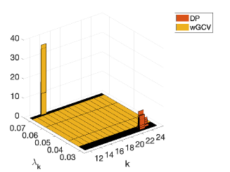
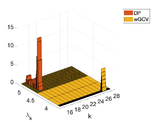
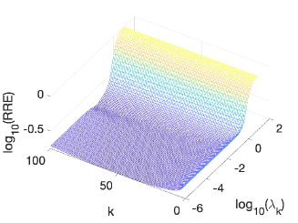
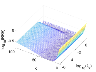
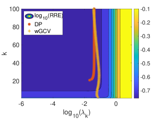
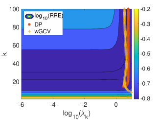
We use the image deblurring and tomography test problems from Section 2 to show how different regularization parameter selection methods can perform within hybrid projection methods. Relevant quantities are displayed in Fig. 8. For both test problems, looking at the frames displayed in the top row, we can infer that both the discrepancy principle and the wGCV method exhibit consistent behavior within different noise realizations; looking at the frames displayed in the middle and bottom rows, we can see that there are clear combinations of values of and that deliver minimal relative reconstructions error norms, and that both the discrepancy principle and wGCV are able to compute couples that eventually (for big enough) lay in such regions. We emphasize that every problem is different, and there is not one approach that will work for all problems. Thus, it is good to have a variety of methods that can guide one in selecting a suitable set of parameters.
| deblurring | tomography |
|---|---|
 |
 |
 |
 |
 |
 |
3.3.3 SVD formulations of quantities used for regularization parameter selection
Notice that in many of the regularization parameter selection strategies, a nonlinear optimization or root finding problem must be solved to estimate . For smaller problems (e.g., the projected problem in hybrid projection methods), the SVD can be exploited for efficient computation of the norm of the approximation solution, the norm of the residual, and the trace of the influence matrix, which all depend on . We remark that these efficiencies are especially impactful when quantities need to be computed for many regularization parameters (e.g., to obtain a representative -curve) or when the projected problem is significantly smaller than the size of the original problem (e.g., ). In this section, we provide SVD formulations for these quantities for Tikhonov regularization, but remark that similar derivations can be made for any spectral filtering method (e.g., TSVD) used to solve the projected problem in a hybrid projection method.
Let the SVD of be given as in Eq. 20 and let
notice that these contain orthonormal columns. Then the solution of the regularized, projected problem Eq. 22 has the form
The ‘influence matrix’ Eq. 23 can then be represented as
Using the above formulas, the squared norm of the solution can be represented as
and the trace of the influence matrix takes the form
To obtain an expression for the norm of the residual, we exploit the fact that and that contains orthonormal columns to get
Let with elements , then
3.3.4 Methods that exploit the links between GKB and Gaussian quadrature rules
All the parameter choice rules for presented so far involve at least one evaluation of a quadratic form of the matrix or . These forms can be expressed as particular Riemann-Stieltjes integrals (written in terms of the SVD of ), which can then be approximated by Gauss or Gauss-Radau quadrature rules. The latter are related to the symmetric Lanczos algorithm, which is itself related to the GKB algorithm; see Section 3.2.1. When dealing with large matrices whose SVD cannot be computed, these relations are crucial to provide computationally affordable approximations of the original quadratic forms in terms of quantities (such as the upper bidiagonal ) generated at the th GKB iteration. Under some additional assumptions, it can be proven that such approximations are upper or lower bounds, which get increasingly accurate as increases. Such connections are underpinned by a solid and elegant theory. In the following we will mention some basic facts without providing many motivations: these are fully unfolded in, e.g., [98]. In the framework of hybrid projection methods, besides using GKB iterations to compute an approximation of the regularization parameter for the Tikhonov problem Eq. 7 according to some rule, GKB is also employed to define the th projected problem Eq. 17 or Eq. 18.
Since all the parameter choice rules described for Tikhonov regularization in Section 3.3.1 and Section 3.3.2 involve the discrepancy norm , and since
| (34) | |||||
in the following we provide the details of the approximation of such a quadratic form and for an overdetermined (i.e., ) only. Considering the eigendecomposition given in terms of the SVD of Eq. 8, and setting
it can be shown that
| (35) |
where the discrete measure is a non-decreasing step function with jump discontinuities at the ’s and at the origin. It is well-known that the above integral can be numerically approximated using a Gaussian quadrature rule, whose nodes are the zeros of a family of orthonormal polynomials with respect to the inner product induced by the measure . Such polynomials satisfy a three-term recurrence relation whose coefficients coincide with the entries of the tridiagonal matrix computed by the symmetric Lanczos algorithm applied to with initial vector (specifically, the entries on the th column of such tridiagonal matrix define the th orthonormal polynomial). Note that such decomposition can be conveniently obtained from the partial GKB decomposition, as shown in Eq. 15.
Consider the eigendecomposition given in terms of the SVD . Then it is well-known that the -point Gauss quadrature rule for approximating Eq. 35 is given by
| (36) | |||||
i.e., the quadratic form evaluated with respect to the projected matrices. The -point Gauss-Radau quadrature rule for approximating Eq. 35, with one node at the origin, can be evaluated similarly, replacing the matrix by the matrix , where is computed at the st GKB iteration. That is,
| (37) |
Since defined in (34) is a -times differentiable function, the quadrature errors associated with the -point Gauss and Gauss-Radau quadrature rules (i.e., with and , respectively), are given by
where , and the ’s and the ’s denote the nodes of the Gauss and the Gauss-Radau quadrature rules, respectively. Since and for , the Gauss-Radau quadrature rule Eq. 37 is an upper bound for , while the Gauss quadrature rule (36) is a lower bound for .
The idea of exploiting Gaussian quadrature to approximate functionals used to set the Tikhonov regularization parameter was first presented by Golub and Von Matt [103], with derivations specific for GCV. This investigation can be regarded as a particular case of the broader explorations of the links between some Krylov methods and Gaussian quadrature conducted by Golub and collaborators; see again [98] for a complete overview of the accomplishments in this area. An important remark concerning GCV is that a different treatment is needed to derive bounds for the numerator and denominator of the GCV function Eq. 32: since a trace term appears in the denominator, a randomized trace estimator can be used to compute its approximation (see, e.g., [103, 189]), while Gauss-quadrature bounds can be used to handle the numerator. Note however that, in [103], a similar approach is adopted to set the regularization parameter for the full-dimensional problem Eq. 7, i.e., the value of so approximated is then used to solve a Tikhonov-regularized problem. For this reason, this approach cannot be properly regarded as a hybrid solver, according to the framework adopted in this paper, although its adaptation would be quite natural. To the best of our knowledge, Gaussian-quadrature-based regularization parameter choice strategies were first adapted to work within hybrid solvers in [33]: here the algorithm involved in setting the regularization parameter according to GCV is identical to the one described in [103], and the computations performed to approximate the numerator of the GCV functional in Eq. 32 are then also employed to define an approximation subspace for the solution (of increasing dimensions), effectively making this approach a hybrid solver. A similar strategy, still tailored to GCV, is presented in [73].
Regularization parameter choice rules for hybrid methods that exploit the links between GKB and Gaussian quadrature rules are especially successful and well-understood when the -curve is employed. This instance of the -curve criterion is sometimes referred to as ‘-ribbon’; see, e.g., [34, 43]. Indeed, in this setting, Gauss and Gauss-Radau quadrature rules provide computationally inexpensive upper and lower bounds (i.e., boxes) for each point on the -curve associated to the full-dimensional Tikhonov problem. Since the -curve bounds are nested (i.e., they become more and more accurate as the number of GKB iterations increases), when the -ribbon is narrow it is possible to infer the approximate location of the ‘vertex’ of the -curve from its shape. For hybrid methods, the -ribbon may first conveniently determine narrow bounds for the (direct) Tikhonov -curve (thereby performing a suitable number of GKB iterations), and then easily locate the approximate vertex of the -curve.
Most recently, the authors of [82] introduce a new principled and adaptive algorithmic approach for regularization, which provides reliable parameter choice rules by leveraging the framework of bilevel optimization, and the links between Gauss quadrature and GKB.
3.4 Theoretical insights
The goal of this section is to give the reader a flavor of the types of theoretical results that have been investigated and their significance for hybrid projection methods.
Project-then-regularize versus regularize-then-project
For standard Tikhonov regularization, an insightful result deals with characterizing the iterates from a hybrid projection method. For a fixed regularization parameter, there is an important result regarding the equivalence of iterations from two approaches: ‘first-regularize-then-project’ and ‘first-project-then-regularize’ [114, 118]. See Fig. 9 and the following theorem.
Theorem 3.1.
Fix and define to be the th iterate of conjugate gradient applied to the Tikhonov problem,
Let be the exact solution to the regularized, projected problem
where and are derived from GKB applied to the original problem. Then
The significance of this result is that, for large-scale problems where the ‘first-regularize-then-project’ approach is not feasible (e.g., because obtaining a good regularization parameter is too expensive a priori, see Fig. 5), the hybrid projection methods that follow the ‘first-project-then-regularize’ approach produce, at the th iteration, the same regularized solution (in exact arithmetic and with the same regularization parameter). Extensions of this result to the case where TSVD regularization is used instead of Tikhonov can be found in [145].
Projection results
Since the approximation subspace for the solution plays a pivotal role in the success of both purely iterative and hybrid projection methods, there have been recent investigations on subspace approximation properties, including results quantifying how much the approximation subspace can be expanded, or how the noise in the data affects the approximation subspace. In particular, the authors of [91] prove that, when GKB is applied to a severely ill-posed problem with noiseless data, the product of the entries of the last column of the bidiagonal matrix decays as ; note that these entries are somewhat related to how much the Krylov subspace is expanded at the th iteration. Under similar assumptions, when employing the Arnoldi algorithm, the rate of decay of the last entry of the Hessenberg matrix (i.e., ) is comparable to . The authors of [127] study how noise in the measurements (right-hand side of Eq. 1) propagates to the projected problem and, in particular, how it enters the basis vectors spanning the approximation subspace. This leads also to efficient estimates of the noise level that can be used to set the regularization parameter for hybrid methods, or a stopping criterion (see Section 3.3). Specifically, assuming that the Discrete Picard Condition holds, the noise amplification (i.e., the appearance of high frequency noise) is described as an effect of damping the smooth components due to convergence of Ritz values to large eigenvalues of and the orthogonalization in the GKB algorithm. After the noise has ‘revealed’ itself in the so called ‘noise-revealing’ iteration, the LSQR relative residual can be used as a noise level estimator. This investigation is extended in [126], to consider the most popular iterative solvers based on GKB and to establish explicit relations between the noise-contaminated bidiagonalization vectors and the residuals of the considered regularization methods. In particular, it is shown that the coefficients of the linear combination of the computed bidiagonalization vectors reflect the amount of propagated noise in each of these vectors; influence of the loss of orthogonality is also discussed. Some of these investigations (most relevantly, the analysis of the residual vector) have been also performed in [90, 89] for methods based on the Arnoldi algorithm, mainly using tools from approximation theory. Finally, the propagation of noise in the approximation subspace and the residuals associated to purely iterative methods based on the GKB algorithm (such as LSQR) and the Arnoldi algorithm (such as GMRES and RRGMRES) is studied in [135]. The latter may not be successful in filtering the noise out, because of the so-called ‘mixing’ of the SVD components in the approximation subspace; this issue may actually be irrelevant, if features of the solution can be reconstructed anyway thanks to the presence of favourable vectors in the Krylov approximation subspace and it can be mitigated using some ‘preconditioning’ [120]; see also Section 4.1. Some ‘preconditioners’ that can be used together with (RR)GMRES to correct for severe asymmetries in the discretized forward operator are proposed and analyzed in [87]. Focusing on image deblurring problems, and exploiting the two-dimensional discrete cosine transform, [121] also analyzes how noise from the data enters the solution computed by LSQR, GMRES, RRGMRES, MINRES, and MR-II, concluding that the noise mainly affects the reconstructions in the form of low-pass filtered white noise, and discouraging the use of GMRES and MINRES for image deblurring.
Other classes of results pair the analysis of the approximation subspace for the solution with the analysis of the behavior of the projected problem, or focus solely on the latter, including results on the approximation of the singular value decomposition, which shed light on how the ill-conditioning of the original problem transfers to the projected problem, on the semi-convergence phenomenon, and on how properties such as the so-called discrete Picard condition are ‘inherited’ by the projected problem. Bounds on the ‘residuals’ associated to the SVD approximations obtained by the GKB and Arnoldi decompositions (i.e., the matrix 2-norm of the difference between the original coefficient matrix Eq. 8 and the approximated SVD obtained at each step of a Krylov subspace method) are presented in [91], where it is concluded that, depending on the method and on the residuals, these could either be 0, or their norm may decay as the singular values of the original coefficient matrix. The authors of [89] prove that, starting from a full-dimensional problem satisfying the discrete Picard condition (i.e., typically assuming noise-free data), the discrete Picard condition continues to hold when the problem is projected using the Arnoldi or the GKB algorithms: this is achieved by combining some SVD update rules and a backward induction argument (i.e., going from the full-dimensional problem to projected problems of decreasing dimension). Naturally, much analysis focuses on establishing theoretical and heuristic links between the performance of TSVD (which can be regarded as a least-squares solver projecting the full-dimensional problem Eq. 9 onto the subspace spanned by the dominant right singular vectors) and Krylov projection methods. Some early investigations, such as [113], find that, since the projection attained with the LSQR method is tailored to the specific right-hand side , this results in a more rapid convergence of the solver. Also, when it comes to computing TSVD-like approximations, the authors of [17] exploit a classical property of GKB (namely, the approximation quality depends on the relative distance between the singular values of [185]) to conclude that, since for discrete inverse problems the relative gap between large singular values of is generally much larger than the relative gap between its small singular values, the singular values of converge very quickly to the largest singular values of . Also, links between the TSVD and Lanczos algorithms (for symmetric problems) are investigated in [92] where, thanks to the speed at which the nonnegative subdiagonal entries of decay to zero, the solution of the discrete ill-posed problems can be efficiently and effectively (i.e., without significant, if any, reduction of the quality of the computed solution) expressed in terms of the Lanczos basis vectors rather than the eigenvectors of ; this extends to the solution subspace determined by LSQR and the right singular vector subspace. More recently, a body of papers by Jia and collaborators puts some renewed emphasis on the investigation of the relations between the TSVD solutions and the solutions computed by some popular purely iterative regularization methods (such as LSQR, LSMR, and MINRES). In particular, assuming distinct singular values, [132] establishes bounds for the distance between the -dimensional Krylov subspace associated to LSQR and the -dimensional dominant right singular space associated to TSVD, and concludes that the former better ‘captures’ the latter for severely and moderately ill-posed problems than for mildly ill-posed problems. This implies that LSQR performs better as a stand-alone regularization method for severely and moderately ill-posed problems, but should be paired with additional regularization (i.e., in a hybrid framework) for successfully handling mildly ill-posed problems. Estimates for the accuracy of the rank- approximation generated by GKB are also provided. This topic is further investigated in [137, 136], where an analysis of the approximation of the large singular values of by the Ritz values is also performed to assess if this happens in natural order (i.e., largest singular values first). The paper [138] extends the same investigations to the case of multiple singular values, with similar findings.
Continuous formulations
Although the present survey paper considers discrete inverse problems, in many situations (especially when analyzing some convergence properties of solvers or inferring the behavior of the projected problems) looking at the continuous formulation (i.e., within a Hibert space ) can be beneficial. Indeed, it is well known that some discretization schemes (e.g., those based on boundary element methods) actually project the continuous problem onto finite dimensional vector spaces, and that such a projection has a regularizing effect; see [114, 145]. Indeed, with ‘proper conversion’, many of the presented derivations for Krylov methods in finite dimension can be translated to the continuous setting; see [70]. CG was historically among the first Krylov methods to be analyzed in a continuous setting: [70] reports relevant results and references. More recently, the authors of [39] show that, when the error-free data vector lies in a finite-dimensional a finite-dimensional Krylov subspace, then the (continuous) GMRES method is a regularization method if the iterations are terminated by a stopping rule based on the discrepancy principle. Methods based on the Arnoldi algorithm (either FOM or GMRES) have been analyzed in a continuous setting [163]: here, some of the properties described (and somewhat heuristically justified) in a discrete setting in [91] are fully established (and sometimes strengthened) in a continuous setting. More specifically, assuming that we are dealing with Hilbert-Schmidt operators (like Fredholm integral equations of the first kind with square-integrable kernels), it can be shown that the rate of convergence of these solvers is related to the extendibility of the Krylov subspace , which is also comparable with the rate of decay of the singular values of . Moreover, it is proven that the dominant singular values can be approximated with improved accuracy as the iterations proceed, further supporting the statement that methods based on the Arnoldi algorithm are regularization methods. This investigation has an impact on the finite-dimensional setting, too: for instance, having proven convergence of the SVD approximation obtained by the Arnoldi algorithm, implies that many parameter choice rules that are intrinsically based on the success of this approximation (see Section 3.3) are meaningful when used within hybrid methods. An analogous investigation appeared in [49], where the infinite-dimensional GKB algorithm and LSQR are considered. The same author considers in [164] the case of Krylov solvers applied to general-form Tikhonov regularization (still in a continuous setting), with a fixed regularization parameter; both solvers based on the Arnoldi algorithm and on the GKB algorithm are considered and the resulting scheme is dubbed ‘ Krylov-Tikhonov’. Denoting by and the solution to the continuous problem and the Krylov solution, respectively, the main investigation in [164] is concerned with proving that such Krylov methods are orthogonal projection methods for the linear operator equation associated to the normal equations for the continuous Tikhonov formulation: because of this, there exists a (semi)norm in such that converges to zero as goes to infinity.
4 Extensions
The goal of this section is to describe some extensions and recent advancements in hybrid projection methods. In particular, in Section 4.1 we describe various hybrid projection methods that have been developed for general-form Tikhonov regularization. In Section 4.2 we describe hybrid projection approaches that go beyond the standard projection subspaces by enrichment, augmentation and recycling of approximation subspaces for the solution. Then in Section 4.3 we go beyond 2-norm regularization and consider the regularized problem. In particular, we focus on recent advancements in flexible iterative methods (which are related to flexible preconditioning where the preconditioner changes during the iterative process) and extensions to hybrid frameworks. In Section 4.4 we describe the increasingly important role that hybrid iterative methods play in the field of large-scale computational uncertainty quantification. We first give a brief introduction to draw connections between traditional variational regularization and statistical (Bayesian) inverse problems, and we describe various scenarios where hybrid projection methods have enabled researchers to go beyond point estimates and perform efficient UQ. In Section 4.5, we describe the role that hybrid projection methods have played in solving nonlinear inverse problems, where the forward model is nonlinear.
A common theme in all the following subsections is that extensions of hybrid projection methods beyond the standard approaches described in Section 3, in order to be effective in a large-scale setting, require the efficient computation of an appropriate solution subspace and adaptive regularization parameter choice for the projected problem (i.e., within the solution subspace), giving rise to hybrid formulations. Although the computed solution subspaces may not be as straightforward as standard methods, they can incorporate some prior knowledge or meaningful information about the solution or the kind regularization functional to be considered, eventually leading to superior reconstructions with respect to the ones delivered by standard methods. Most often this means that the standard GKB or Arnoldi decompositions have to be modified, for example, to formally work with variable preconditioning, to enforce orthogonality or optimality properties in a different norm, or to incorporate a low-dimensional subspace representing prior information. Also, most often, such tools have already been developed for use in other settings, e.g., for the solution of well-posed problems (e.g., PDEs). Therefore, a considerable part of this section is devoted to reviewing such tools, tailoring them to the problems at hand, and drawing possible analogies between them.
4.1 Beyond standard-form Tikhonov: Hybrid projection methods for general-form Tikhonov
Thus far we have focused mainly on the standard-form Tikhonov problem (7), where the regularizer enforces an overall small norm for the solution; however, other smoothness properties may be desired. Many researchers have considered the general-form Tikhonov problem,
| (38) |
where is called the regularization matrix. We assume that the null spaces of and intersect trivially, so that has full column rank and the solution to (38) is unique. Typical choices of include discretizations of a differential operator (e.g., the discrete first or second derivative). An important observation is that the general-form Tikhonov solution can be written as a spectral filtered solution, where both the filter factors and the basis for the solution are determined by the generalized singular value decomposition (GSVD) of ; see, e.g., [118, Chapter 8]. However computing the GSVD is not always feasible, e.g., for large-scale unstructured problems. In these settings, the most immediate approach is to apply an iterative solver (e.g., any of the solvers listed in Section 2.2) to the equivalent least-squares formulation of (38): however, a suitable value of must be fixed ahead of the iterative method. Since this is typically not the case, one should apply an iterative solver to Eq. 38 repeatedly (once for every tested value of ), as dictated by some well-known parameter choice strategies (such as the ones listed in Section 3.3): this eventually results in a costly strategy, and alternatives have been sought in the literature.
A common approach to handle the general-form Tikhonov problem is to transform it to standard form [68]. That is, one computes
| (39) |
and where is the component of the regularized solution in the null space of . Here is the -weighted generalized inverse of , defined by ; see [117, Section 2.3]. Note that, if is invertible, then , and, if has full column rank, then . If is an underdetermined matrix, then may not be the same as . In the Bayesian inverse problems literature (see Section 4.4), this particular change of variables is referred to as priorconditioning [45, 32, 46, 35], because the matrix is constructed from the covariance matrix of the solution modeled as a random variable (see also Section 4.4.1). The main idea is to interpret as a preconditioner; however, while preconditioning for iterative methods is often discussed in the context of accelerating iterative methods (typically via clustering of the eigenvalues), priorconditioners in Eq. 39 change the subspace for the solution by including information from the prior. Indeed, in earlier work that leveraged this idea without collocating it within the Bayesian framework, this approach was dubbed ‘smoothing norm preconditioning’ and was first adopted in connection with CGLS [114], and then GMRES [120]. For regularization functionals designed to promote edges, Krylov subspace methods may have poor convergence whereas the transformed problem amplifies directions spanning the columns of the prior covariance matrix, thereby improving convergence [5]. Once formulation Eq. 39 is established, hybrid projection methods can be applied, which define the approximation subspace for the solution with respect to the matrix . For instance, in the case of GKB, the th approximation subspace for the solution is defined as follows:
Correspondingly, the th iteration of the LSQR algorithm updates the matrix recurrence
where is lower bidiagonal, has orthonormal columns that span , and has orthonormal columns with . Imposing in (39), i.e., taking , and exploiting unitary invariance of the 2-norm, the objective function in (39) can be equivalently rewritten as the -sized least-squares problem
| (40) |
For fixed , any suitable parameter choice strategy can be used on the projected problem (40) to choose . If is computed at fixed pre-sampled values of (e.g., when the -curve criterion is adopted), this may be done with short term recurrences on the iteration (i.e., in , for fixed ), without storage of ; see Section 3.3 and [145] for details. However, in general, should be assumed small enough, so that problem Eq. 40 can be efficiently generated and solved. For some problems, multiplication with can be done by solving a least-squares problem followed by an oblique projection; see [116, 120] for details. Furthermore, there are some regularization operators for which sparsity or structure can be exploited so that multiplications with can be done efficiently (e.g., banded matrices, circulant matrices, and orthogonal projections [44, 69, 154, 179]). However, in general, performing multiplications with may be computationally difficult especially for large-scale problems (e.g., when is defined as a product of matrices or as a sum of Kronecker products).
In the framework of hybrid projection methods, alternative approaches to approximate the solution of (4.1) have been devised without resorting to a standard-form transformation. For instance, Kilmer, Hansen and Español [144] developed a hybrid projection method that simultaneously bidiagonalizes both and (here can be rectangular and does not need to be full rank), using a joint bidiagonalization algorithm inspired by Zha [218]. More precisely, a partial joint bidiagonalization for and is updated at each iteration: at the th iteration, it reads
| (41) |
where , , and . Although this algorithm only requires that products with and their transposes can be computed, the cost of generating the partial factorization Eq. 41 is somewhat difficult to quantify: indeed, the th step requires one call to LSQR to produce orthogonal projections that are needed to update the partial joint bidiagonalization (41), and each LSQR iteration requires four matrix-vector products (with each of , , , and ). Taking , i.e., , in Eq. 38 results in the following equivalent problems
| (42) |
Since the last problem in the above equations is a Tikhonov problem of dimension involving only bidiagonal matrices, it is significantly cheaper to solve than Eq. 38, especially for small. Let us denote by the minimizer of Eq. 42, then is the minimizer of Eq. 38, constrained to . For fixed , the joint bidiagonal structure leads to short recurrence updates (in ) for , for the residual norm , and for the regularization norm term : this is relevant if the solution has to be computed at fixed pre-sampled values of , e.g., when applying the -curve criterion. The discrepancy principle to set adaptively at each iteration can also be efficiently employed. It can be shown that the approximation subspace is meaningful, as ‘resembles’ a truncated GSVD regularized solution to Eq. 1.
Reichel, Sgallari, and Ye [175] describe an iterative approach that simultaneously reduces square matrices and to generalized Hessenberg matrices using a generalized Arnoldi process, originally introduced in [152]. The formal full factorizations associated to this method consist of
| (43) |
and where is orthogonal. In practice, iterations of the generalized Arnoldi algorithm can be computed with initial vector to generate the first columns of the generalized Hessenberg matrices and appearing above, and the corresponding columns of . The columns of span a so-called generalized Krylov subspace obtained by multiplying by and in a periodic fashion. Let and be the principal submatrices of the matrices and , and let be obtained by taking the first columns of . Taking , i.e., , in Eq. 38 results in the following equivalent problems
Note that the approximation subspace for the solution of Eq. 38 can alternatively be generated starting from , leading to minor adjustments in the above projected problem (analogous to the range-restricted approach described in Section 3.2.1). Similar to the method in [144], the present approach allows adaptive selection of the regularization parameter at the th iteration, with a negligible computational overhead. Different from [144], the present method can work only if both and are square (but this restriction can be overcome, e.g., by zero-padding). Furthermore, the present method does not require the action of and , and no (inner) calls to LSQR are needed to generate the factorization Eq. 43. While these are clear advantages of the solver presented in [175] compared to that presented in [144], the downsides are that the structure of the generalized Hessenberg matrices and cannot be immediately exploited (as was possible for bidiagonal matrices and in Eq. 41); moreover, to the best of our knowledge, no heuristic insight is available to justify the choice of the approximation subspace for the solution (in particular, no links with truncated GSVD have been established). Despite this, some specific features of the solution of Eq. 38 can be enhanced by pairing the present method with so-called ‘selective regularization’, i.e., by augmenting the approximation subspace for the solution associated to this specific method; generic (i.e., not specific to the generalized Arnoldi algorithm) schemes for achieving augmentation are described in Section 4.2.
Lampe, Reichel, and Voss [147] propose an alternative projection method for approximating the solution (38), which is initiated by picking an approximation subspace of small dimension spanned by the orthonormal columns of a matrix . This can be done, for instance, by running GKB iterations, so that . Denote by the solution of the constrained Tikhonov problem obtained by imposing in Eq. 38, i.e., take , where
Note that can be computed efficiently by using a ‘skinny’ QR factorization of , which can be updated as increases. A suitable value of the regularization parameter can be determined using any of the strategies described in Section 3.3. Once is computed, the original search space is expanded by the normalized gradient of the functional in Eq. 38 evaluated at . Namely, one considers
Although so defined is orthogonal to , this can be enforced numerically using reorthogonalization techniques, if loss of orthogonality is a concern. In general, the approximation subspace for the solution of Eq. 38 is not a Krylov subspace and it is therefore called a ‘generalized Krylov subspace’: note however that it is yet a different generalized Krylov subspace than the one used in [175]. The process of solving problem Eq. 38 constrained to the updated approximation subspace is repeated, and expansions of are generated until a stopping criterion is satisfied.
Hochstenbach and Reichel [128] use a partial GKB built with respect to and to generate, at the th iteration, the solution subspace , onto which they project the regularization matrix in order to compute an approximate solution. A similar idea was used in [210, 91]. Note that, contrary to all the strategies summarized so far in the present section, when using these approaches, the matrix does not enter the approximation subspace for the solution.
4.2 Beyond standard projection subspaces: Enrichment, augmentation, and recycling
The success of Krylov projection methods, and in particular the regularizing properties of Krylov methods, depends on the ability of the associated Krylov subspace to capture the most salient features of the solution. In the previous section, we surveyed approaches to solve the general-form Tikhonov problem Eq. 38, where the choice of the matrix may affect the solution subspace for the iterative method (e.g., via subspace preconditioning or priorconditioning with a change of variables). Such transformations result in a Krylov subspace that is ‘better suited’ for the problem [45, 120]. This means that the approximate solution vectors can capture the essence or important features of the solution, which can lead to faster convergence properties since fewer iterations are needed to obtain an accurate solution. However, in some applications, the regularized solution can be further improved by extending or enhancing the approximation subspace via enrichment, augmentation, and recycling techniques.
We begin with some motivating scenarios where such techniques may be desired. First, experienced practitioners may have solution vectors containing important information about the desired solution (e.g., a low-dimensional subspace) from previous experiments or theoretical analyses. By incorporating these solution basis vectors, the solution accuracy can be significantly improved, depending on the quality of the provided vectors. Second, for very large inverse problems where many iterations are needed or where there are many unknowns, one of the main computational disadvantages of most hybrid methods compared to standard iterative methods is the need to store the basis vectors for solution computation, namely (using the same notations as in Eq. 19). Furthermore, for problems with slow convergence, implicit restarts and augmentation can speed up convergence without affecting memory. Third, and this is related to Section 4.5, hybrid methods may be embedded within larger frameworks, e.g., optimal experimental design [110, 108] or nonlinear inverse problems [107]. A sequence of inverse problems must be solved, e.g., where the forward model may be parameterized such that the change in the model from one problem to the next is relatively small, or the goal may be to compute and update solutions from streaming data. Rather than start each solution computation from scratch, recycling techniques can be used to improve the given subspace and to compute a regularized solution efficiently in the improved subspace. In the context of solving inverse problems, we describe extensions that go beyond the standard projection subspaces.
We split our discussion into two main classes: (1) enrichment methods and (2) augmentation or recycling approaches. For both classes of methods, we assume that we are given a low-dimensional subspace that represents prior information or expert knowledge. That is, we assume that we are given a suitable set of basis vectors, denoted , such that a well-chosen subspace for the solution is given by . We call this the ‘prior solution subspace’ (not to be confused with priors or priorconditioning methods). The main assumption is that the solution has a significant component in the given subspace , and the goal is to incorporate the provided subspace judiciously in order to obtain improved regularized solutions.
Enrichment methods
We begin with enrichment methods, which we define as methods that, at the th iteration, compute regularized solutions in a solution subspace that is a direct sum of the prior solution subspace and a standard -dimensional Krylov subspace, i.e.,
| (46) |
That is, hybrid projection methods with enrichment construct iterates defined as
| (47) |
Enrichment methods can improve the solution accuracy by incorporating information about the desired solution into the solution process, i.e., by enriching the solution subspace. Methods for enriching Krylov subspaces have been described in the context of both Arnoldi and Lanczos projection methods.
For Arnoldi based methods, the Regularized Range-Restricted GMRES method (R3GMRES) [66] extends the RRGMRES approach (see Section 3.2.1) to include a subspace that represents prior information about the solution where the approach is to compute as as in Eq. 47 with . Efficient implementations are described in [66].
For Lanczos-based projection methods, enrichment methods seek solutions of the form Eq. 47 where the solution space is given by Eq. 46 with . A modification of CGLS method (sometimes also denoted in the literature with the acronym CGNR) was described in [42], where Krylov subspaces are combined with vectors containing important information about the desired solution (e.g., a low-dimensional subspace). Given an enrichment subspace , the enriched CGLS method determines the th iterate in the subspace The enriched CGLS method was used for Tikhonov problems (e.g., penalized least-squares problems), where several linear systems were solved for different choices of the regularization parameter as described in Frommer and Maass [78]. More specifically, a sequence of Tikhonov problems for regularization parameters for are solved, until for some the corresponding solution satisfies the discrepancy principle. A hybrid enriched bidiagonalization (HEB) method that stably and efficiently augments a ‘well-chosen enrichment subspace’ with the standard Krylov basis associated with LSQR is described in [119]. The idea is to use the Lanczos bidiagonalization algorithm to compute an orthonormal basis, and augment it by a user-defined low-dimensional subspace that captures desired features of the solution in each step of the algorithm.
Finally, we remark that a subspace-restricted SVD was described in [129], where a modification of the singular value decomposition permits a specified linear subspace to be contained in the singular vector subspaces. That is, the user can prescribe some of the columns of the and matrices for all truncations, and truncated versions as well as Tikhonov problems can be solved. For inverse problems, such approaches can give more accurate approximations of the solution when compared to standard TSVD and Tikhonov.
Augmentation and recycling techniques
The development of augmentation schemes is deeply intertwined with the development of recycling techniques, in particular, Krylov subspace recycling methods for solving sequences of linear systems with slowly changing coefficient matrices, multiple right hand sides, or both. We point the interested reader to recent surveys [200, 199] and references therein. Subspace recycling methods can exhibit accelerated convergence by enabling effective reuse of subspace information that is typically generated during a Krylov method on one or more of the systems. For example, for well-posed least-squares problems that require many LSQR iterations, augmented LSQR methods have been described in [9, 6] that augment Krylov subspaces using harmonic Ritz vectors that approximate singular vectors associated with the small singular values, which can reduce computational cost by using implicit restarts for improved convergence. However, when applied to ill-posed inverse problems, the augmented LSQR method without an explicit regularization term exhibits semi-convergent behavior. Thus, in this setting, the goal is not so much to recycle spectral information for faster convergence, but rather to augment a solution space to include certain known features about the solution.
Next, we provide an overview of augmented Krylov methods for solving ill-posed problems with a specific focus on hybrid methods. Suppose we are given a general -dimensional subspace , where has orthonormal columns, and define and to be the orthonormal projectors onto and respectively. The decomposition approach described in [8] and the augmented Krylov methods split the solution space such that the solution at the th iteration is partitioned as
It is assumed that the augmented space is small (e.g., ) and does not require regularization, thus a direct method can be used to compute To compute , an iterative method is used. More specifically, let
| (48) |
be the ‘skinny’ QR factorization, where contains orthonormal columns and is upper triangular. Then the approximate solution for the augmented GMRES approach is obtained by solving the constrained least-squares problems,
similarly, the augmented RRGMRES method solves
More details are given in [8, 7]. Augmented LSQR methods have been described in [9, 6].
A general framework to combine a recycling GKB (recycling GKB) process with tools from compression in a hybrid context are described in [139]. More specifically, the approach consists of three steps. First, a suitable set of orthonormal basis vectors is provided (e.g., from a related problem or from expert knowledge) or may need to be determined (e.g., via compression of previous solutions). This prior solution subspace may even include an initial guess for the solution. The second step is to use a recycling GKB process to generate the columns of that span the Krylov subspace
where and is defined in Eq. 48. The third step is to find a suitable regularization parameter and compute a solution to the regularized projected problem in the extended solution space. The recycled, hybrid iterate is given by
This process can be repeated in a cyclic fashion, and it is successful in solving a broad class of inverse problems (e.g., solving very large problems where the number of basis vectors becomes too large for memory storage, solving a sequence of regularized problems (e.g., changing regularization terms or nonlinear solvers), and solving problems with streaming data).
Let’s compare and contrast
For all of the described methods, the improvement in solution accuracy significantly depends on the quality of the provided prior solution subspace vectors . Thus, we reiterate that the major advantage as well as the major concern for all enrichment, augmentation, and recycling methods is that the augmented subspace needs to be chosen appropriately, i.e., problem-dependent or prior information about the solution needs to be known. The performance of these methods compared to standard methods will depend on the amount of relevant and important information about the solution that is encoded in the given subspace. Some suggestions for subspaces are provided in [129, 139]. For problems with unsuitable augmentation spaces, an adaptive augmented GMRES was considered in [146], which automatically selects a suitable subspace from a set of user-specified candidates.
The main difference between enrichment methods and augmentation methods lies in how the solution space is constructed. Iterates of enrichment methods belong to a direct sum of the prior solution subspace and a standard Krylov subspace, whereas the generated subspace for augmented methods is restricted to the orthogonal complement of It may be argued that since augmentation and recycling methods generate subspace vectors that incorporate the provided prior solution subspace, these methods can improve on the generated space. However, this observation is problem dependent. Further investigations regarding the relationship between spaces and can be found in [66].
We also mention that there have been various works on developing hybrid methods for solving systems with multiple right hand sides. In [167], the authors suggest using the block Lanczos algorithm [97]. Some more recent work on extending generalized hybrid methods for multiple right hand sides exploit global iterative methods [206] and block reduction methods [2]. Such approaches have been considered for solving dynamic inverse problems [58]. Furthermore, there is recent work on developing hybrid projection methods based on tensor-tensor products and applications to color image and video restoration [178, 177].
4.3 Beyond the 2-norm: Sparsity-enforcing hybrid projection methods for regularization
Although widely used, it is well known that standard-form Tikhonov regularization Eq. 7 and even its general-form counterpart Eq. 38 can be rather restrictive and that other regularization terms can yield better approximations of in Eq. 1. For example, if is known to be sparse (i.e., when most of its entries , , are expected to be zero), the variational formulation
| (49) |
is commonly considered in the literature, especially since the advent of the compressed sensing theory; see, e.g., [48]. Indeed, while sparse vectors have a small -‘norm’, replacing the -norm in Eq. 49 by an -‘norm’ would yield an NP-hard optimization problem (see, for instance, [77]). A well-established practice is to consider (instead of ) regularization terms with to enforce sparsity, noting that the objective function in (49) is non-differentiable at the origin and it is nonconvex when (see, e.g., [131, 148, 149]). Note that, if sparsity of the solution in a different domain (e.g., wavelets, discrete cosine transform, gradient) is desired, a regularization term of the form should be considered, where is a so-called ‘sparsity’ transform; this situation will be considered in Section 4.3.4. Also, sometimes, an -norm with has to be used to evaluate the fit-to-data term in Eq. 49: this is appropriate, for instance, when the noise term in Eq. 1 is modeled as impulse noise; see, e.g., [27].
The - regularized problem Eq. 49 can be solved using a variety of general nonlinear solvers and optimization methods; see, for instance, [16, 93, 216] and the references therein. Here we focus on solvers that approximate the regularization term in (49) by a sequence of weighted terms (i.e., iteratively reweighted schemes). This approach intrinsically relies on the interpretation of problem (49) as a nonlinear weighted least-squares problem of the form
| (50) |
where the diagonal weights in are defined as
| (51) |
Since we are considering , division by zero might occur if for any and, in fact, this is common situation in the case of sparse solutions. For this reason, instead of (51), we can consider the following closely related weights
| (52) |
where is a parameter that, to keep the derivations simple, we will consider fixed and chosen ahead of the iterations (although some authors adaptively choose it). Problem (50) is then replaced by
| (53) |
where ensures that is differentiable at the origin for . Note that problem (50) can be recovered from problem (53) by setting .
A well-established framework to solve problem (53) is the local approximation of by a sequence of quadratic functionals that gives rise to a sequence of quadratic problems of the form
| (54) |
where , is a constant (with respect to ) term for the th problem in the sequence, and has absorbed other possible multiplicative constants so that in (54) corresponds to a quadratic tangent majorant of in (53) at , i.e., for all , , and ; see also [131, 182]. Because of this, iteratively reweighted schemes (54) can be regarded as particular instances of majorization-minimization (MM) schemes, and convergence to a stationary point of the objective function in problem (53) can be guaranteed; see [131, 133, 148].
The vector denotes the solution of (54). For moderate-sized problems, or for large-scale problems where has some exploitable structure, may be obtained by applying a direct solver to (54). However, for large unstructured problems, iterative solvers can be used in different fashions to approximate the solution of (54): this leads to either schemes based on nested (inner-outer) iteration cycles for the sequence of problems (53) or schemes that adaptively incorporate updated weights at each iteration of a single iteration cycle. The former are detailed in Section 4.3.1, while the latter are detailed in Sections 4.3.2 and 4.3.3.
4.3.1 Strategies based on inner-outer iterations
Iteratively Reweighted Least Squares (IRLS, [20, Chapter 4], [64]) or Iteratively Reweighted Norm (IRN, [105, 182]) methods are very popular schemes that can handle the smoothed reformulation Eq. 53 of problem Eq. 49. Let denote the approximate solution at the th iteration (of an inner cycle of iterations) for the th problem of the form Eq. 54 (i.e., at the th iteration of an outer cycle of iterations); one typically takes when a stopping criterion is satisfied for the inner iteration cycle. IRLS or IRN methods based on an inner-outer iteration scheme are very popular and have been used in combination with different inner solvers, such as steepest descent and CGLS [76, 182].
If is square and invertible (note that this can be assumed when the weights are defined as in Eq. 52 with for any fixed ), problem Eq. 54 can be easily and conveniently transformed into standard form as follows
| (55) |
The interpretation of the matrix as a right preconditioner for problem Eq. 54 can be exploited under the framework of priorconditioning; see Section 4.1 and [32]. Similar to the approaches mentioned for Eq. 54, Krylov methods can be straightforwardly adopted to compute an approximate solution of the equivalent th problem of the form Eq. 55 (i.e., at the th iteration of an outer cycle of iterations) through an inner cycle of iterations. In particular, variants based on hybrid projection methods (such as hybrid GMRES or hybrid LSQR) have been successfully considered, with the added benefit that adaptive regularization parameter choice strategies (based, e.g., on the discrepancy principle, UPRE, and GCV) can be considered; see [181]. Specifically, at the th iteration of a Krylov method for (55), let be the matrix whose columns, span a (preconditioned) Krylov Subspace of dimension ; the precise definition of depends on the selected projection method. Problem (55) can be projected and solved in by computing
| (56) |
so that , and
Once has been computed and once the weights have been updated according to (52), the st problem of the form Eq. 55, with replaced by , needs to be solved: to achieve this, one needs to compute a new Krylov subspace from scratch, defined with respect to the new coefficient matrix . For this reason, this approach may become computationally expensive.
4.3.2 Strategies based on generalized Krylov methods
One way to avoid inner-outer iterations when applying the IRN method described in Section 4.3.1 is to exploit generalized Krylov subspaces (GKS), like the ones described in Section 4.1: this approach underlies the so-called GKSpq [148] and MM-GKS [131] algorithms.
Given the initial subspace generated by the GKB algorithm, where is small (typically ) and has orthonormal columns, at the th iteration of the MM-GKS method, a GKS spanned by the orthonormal columns of is computed, and it is used to define the following projection of problem Eq. 54,
Equivalently, introducing the ‘skinny’ QR factorizations
| (57) |
the above problem can be reformulated as the low-dimensional (if ) problem
After the th approximation to problem Eq. 54 is formed by taking , one computes the residual of the normal equations associated to Eq. 54
The subspace is then expanded by adding the vector ; reorthogonalization of the columns of may be advisable to enforce accuracy. An initial guess for is needed to define the first weights , and the authors of [131] suggest to take , although this only works when is square. We emphasize that the regularization parameter can be adaptively set during the GKS iterations; see [27, 26]. Also, an expression for the quadratic tangent majorant Eq. 54 different from can be devised, which allows for a cheaper GKS computation, in that smart updates of the QR factorization Eq. 57 are performed: we refer to [131] for the details. Finally, such strategies based on GKS can also handle generalizations of problem Eq. 49 where weights are also included in the fit-to-data term.
4.3.3 Strategies based on flexible Krylov methods
Another approach that avoids inner-outer iterations when applying the IRN method described in Section 4.3.1 is to exploit flexible Krylov subspaces (FKS): this approach underlies hybrid methods based on the flexible Arnoldi algorithm [85] and the flexible Golub-Kahan algorithm [51], as well as the more recent IRN-FKS methods [86]. The starting point of this class of methods is the formulation Eq. 55 of the th reweighted problem. Flexible Krylov methods, which are classically employed to handle iteration-dependent preconditioning [162, 186, 197], provide a natural framework to update the inverted weights as soon as a new approximation of is computed. That is, at each iteration, the updated inverted weights are immediately incorporated within the approximation subspace for the solution to the next problem in the sequence.
Formally, both the flexible Arnoldi and the flexible Golub-Kahan algorithms look very similar to their standard counterparts Eq. 13 and Eq. 14, respectively. If is square, taking and defining using an initial guess ( if ), the th iteration of the flexible Arnoldi algorithm [186] applied to problem Eq. 55 computes
| (58) |
where is defined as in (52), being the solution obtained at the previous iteration, and where has orthonormal columns. iterations of the flexible Arnoldi algorithm can be equivalently expressed as the partial matrix factorization
| (59) |
Here the columns of span the approximation subspace for the solution, is defined as in Eq. 58 and, by construction, is upper Hessenberg. If is rectangular, taking , the th iteration of the flexible Golub-Kahan algorithm [51] applied to problem Eq. 55 computes
| (60) |
where the inverted weights are updated as in the flexible Arnoldi case, and both and have orthonormal columns. iterations of the flexible Golub-Kahan algorithm can be equivalently expressed as the partial matrix factorizations
| (61) |
Similar to Eq. 59, the columns of span the approximation subspace for the solution , and are defined as in Eq. 60 and, by construction, and are upper Hessenberg and upper triangular, respectively. We emphasize that, in both Eq. 59 and Eq. 61, is not necessarily a Krylov subspace (see [197]), and interpreting them as standard preconditioned Krylov subspaces is not straightforward (see [162]). As in Section 3, we assume that both Eq. 59 and Eq. 61 are breakdown-free, i.e., at iteration , has dimension . The approximate solution computed at the th iteration is used to update the matrix to be employed to expand the solution subspace at the st iteration, as in Eq. 58 and Eq. 60.
The available strategies [51, 85, 86] that approximate the solution of problem (55) through flexible Krylov methods all compute, at the th iteration,
| (62) |
and essentially differ in the choice of the regularization matrix . Specifically,
- (i)
-
(ii)
One of the methods in [51] (dubbed ‘hybrid-R’) takes , where is the upper triangular factor in the ‘skinny’ QR factorization of the basis vectors, i.e., , which can be efficiently updated for consecutive .
-
(iii)
The methods in [86] take , where is the upper triangular factor in the ‘skinny’ QR factorization of the transformed basis vectors, i.e., . Note that, unless is a multiple of the identity matrix, the QR factorization cannot be efficiently updated for consecutive values of , but it is still feasible to compute if .
The three options above reveal that, when using hybrid projection methods based on flexible Krylov subspaces, even if problem Eq. 54 is transformed into standard form Eq. 55, projecting and regularizing are not interchangeable anymore. Indeed, option (i) corresponds to a ‘first-project-then-regularize’ scheme (i.e., it penalizes the 2-norm of the projected solution ) while option (iii) corresponds to a ‘first-regularize-then-project’ scheme; option (ii) penalizes the 2-norm of the full-dimensional solution . When option (iii) is used, exploiting the majorization-minimization framework allows to prove that the sequence of approximate solutions to Eq. 62 converges to a stationary point of problem (53). Note that, by exploiting the properties of the matrices appearing in Eq. 59 and Eq. 61, the fit-to-data term is equivalently expressed as in the flexible Arnoldi case, or in the flexible Golub-Kahan case. Although the regularization parameter in Eq. 62 is displayed as independent of , a heuristical adaptive choice is possible employing any of the strategies described in Section 3.3. A suitable approximation to a solution of Eq. 49 is efficiently computed if, for small , the columns of can be used to capture the main features thereof.
4.3.4 Sparsity under transform
Many of the methods described above for problem Eq. 49 can be generalized to approximate a solution to the more general variational regularization problem,
| (63) |
All the methods based on inner-outer iterations described in Section 4.3.1 and the methods based on GKS described in 4.3.2 can handle regularization terms of the form : this can be done efficiently if matrix-vector products with are cheap to compute. Note that the discrete (anisotropic) total variation regularization functional,
| (64) |
can be expressed in this framework. When , such regularization terms can be interpreted as enforcing sparsity of the unknown . An IRN method for handling TV-like regularizers was proposed in [215] that employs CGLS during the inner iterations, while [5] uses preconditioned LSQR applied to a problem that is effectively transformed into standard form. The authors of [80] propose an inner-outer iterative method that enhances edges through multiplicative updates of the weights, and which exploits the hybrid projection method based on joint bidiagonalization method Eq. 41. The methods based on flexible Krylov subspaces described in Section 4.3.3 can be as well extended to handle problem Eq. 63, but the strategies adopted to achieve this are regularizer-dependent: in other words, no universal approach is possible, even for the special case . For instance, [51] describes an approach that works when is an orthogonal wavelet transform for methods based on both the flexible Arnoldi and the flexible Golub-Kahan algorithms. Also, [81] describe an extension of FGMRES that handles total variation Eq. 64 by first transforming into standard form. Finally, hybrid Krylov projection methods based on either an inner-outer iterative scheme or a flexible scheme, have been used for nuclear norm regularization , which is meaningful when is a vectorization of a low-rank 2D quantity (such as a low-rank 2D image); see [84].
4.4 Beyond deterministic inversion: Hybrid projection methods in a Bayesian setting
Recently, hybrid projection methods have found utility in the framework of statistical inverse problems, within a Bayesian approach. Our goal in this section is to draw important connections between deterministic and statistical inverse problems, so that the reader can understand the role that hybrid projection methods can play in the Bayesian setting. For more detailed descriptions, we refer the interested reader to excellent books and reviews on Bayesian inverse problems [141, 46, 47, 41] and computational uncertainty quantification [11], and references therein.
Traditionally, regularization can be interpreted as a practical approach to replace an ill-posed problem by a nearby well-posed one. For example, Tikhonov regularization was originally motivated as a tool to stabilize the solution process by computing one single deterministic solution of a modified problem [205, 204]; see also Section 2. However, the Bayesian framework also provides a systematic way for solving and analyzing inverse problems by modelling the unknown as a random variable. Although Bayesian inverse problems can be analyzed in a continuous setting [202], here we focus on discrete inverse problems, where the underlying mathematical models have been discretized before applying Bayesian analysis.
In Section 4.4.1 we will draw connections between regularization and Bayesian inversion. In particular, we will show that, under some specific assumptions on the prior, regularized (e.g., Tikhonov) problems arise in the Bayesian framework. One of the main benefits of the Bayesian approach is that different priors can be easily incorporated. Then, in Section 4.4.2, we describe some computational tools for UQ that can exploit hybrid projection methods. These tools bridge developments in the numerical linear algebra community with those in the UQ community for more efficient and practical inversion that can benefit a wide range of applications.
4.4.1 Connections between regularization and Bayesian inversion
First some preliminary notation. Let and be symmetric positive definite (SPD); then, an -variate normally distributed random variable has a density function given by
where denotes the determinant of a matrix and for any and SPD.
Consider the stochastic extension of (1) where , and are random variables. For notational clarity, note that we have dropped the subscript on . Assume that and are independent and normally distributed,
| (65) |
where is the prior mean and and are SPD matrices for the prior and noise respectively. Here we assume that and are known. Although it is typically not necessary to include these parameters (i.e., they can be absorbed in the definition of and ), we include them for clarity and to draw connections to hybrid projection methods in Section 4.4.2.
The probability density function for given is given by
which is also called the likelihood function. Note that the estimate that maximizes the likelihood function (dubbed the maximum likelihood estimator or MLE) is the solution to an unregularized weighted least-squares problem, i.e.,
where is a symmetric (e.g., Cholesky) factorization. Note that if , then we get a standard least-squares problem. The likelihood function is defined solely based on the assumptions from the noise model and extends naturally for nonlinear problems, e.g., if one were to consider a nonlinear forward model, where and , then the MLE estimate is the solution to the nonlinear least-squares problem, . Additive Gaussian noise is the most common noise model used in the literature, but it is worth mentioning that in many applications, such as medical and atmospheric imaging, a Poisson noise model is appropriate. Specifically, in the linear case and assuming independence, ; the likelihood model takes the form
Various noise models can be incorporated, leading to different likelihood functions. For general data-fit terms, hybrid projection methods described in Section 4.3 can be used to approximate the MLE. For the remainder of this section, we consider additive Gaussian noise.
Next, we consider assumptions on prior information about , as described in (65), where the prior density function is given by
Using Bayes’ Theorem, we can derive the posterior density function
| (66) |
where stands for ‘proportional to’. A crucial point to note is that for Bayesian inverse problems, the posterior density function is the solution to the inverse problem. The posterior distribution provides the full information about the distribution of parameters in , given the data . However, for practical interpretation and data analysis, it is necessary to describe various characteristics of the posterior distribution [203]; thus leading to the field of uncertainty quantification. For example, a common goal is to compute the maximum a posteriori (MAP) estimator, i.e., the point estimate that corresponds to the maximum of (66). We denote this as
| (67) | ||||
| (68) |
where the closed form solution in (68) can be obtained by setting the derivative to zero.
Furthermore, it can be shown that, under the above assumptions (linear problem with Gaussian noise and prior), the posterior is indeed Gaussian, where the posterior covariance matrix and the posterior mean (i.e., the MAP estimate) are given as
| (69) |
respectively, with [141].
Next we discuss some examples of priors and show how the posterior distribution and, in particular, the MAP estimate is defined. Gaussian priors are the most common priors used in the literature. We split the discussion into three scenarios. First, for cases where the symmetric factorization of the precision matrix (i.e., the inverse of the covariance matrix) is computationally feasible, i.e., , the MAP estimate is the solution to the optimization problem,
With a simple change of variables, and , the problem reduces to solving
Let : then, this is general-form Tikhonov problem (38), and hybrid projection methods to solve this problem were discussed in Section 4.1. For this scenario, a prevalent approach in the literature models as a sparse discretization of a differential operator (for example, the Laplacian or the biharmonic operator). This choice corresponds to a covariance matrix that represents a Gauss-Markov random field. Since for these choices, the precision matrix is sparse, working with directly has obvious computational advantages.
Second, for the case where application of is feasible (e.g, it is a sparse matrix) but computing the symmetric factorization is too expensive, a factorization-free preconditioned LSQR approach called MLSQR was proposed in [5]. The approach is analytically equivalent to LSQR applied to a preconditioned least-squares problem with the preconditioner , but avoids the factorization by using weighted inner products to implicitly apply the preconditioner. The authors considered applications in the context of nonlinear regularizers.
Third, there are many prior models where the precision matrix and its factorization are not available, but matrix-vector multiplications with can be done efficiently. For example, for Gaussian random fields, entries of the covariance matrix are computed directly as , where are the spatial points in the domain and is a covariance kernel function (e.g., -exponential, or Matérn class). Although there are many modeling advantages, the main challenge is that the resulting prior covariance matrices are often very large and dense; explicitly forming and factorizing these matrices is prohibitively expensive. For such prior models, efficient matrix-free techniques (e.g., FFT embedding and -matrix approaches) can be used, for example, to compute matrix-vector products with the prior covariance matrix . Generalized hybrid projection methods were proposed in [57] to compute Tikhonov regularized solutions (i.e., MAP estimate (67)) effectively. The approach relies on a change of variables and uses a generalized GKB algorithm for projection [4]; note that this is a fundamentally different algorithm than the one presented in Section 4.3.2 for regularization that is based on GKB (for initialization) and some generalization of Krylov projection methods.
Non-Gaussian priors are also common in the literature, but are more challenging to handle. One class of priors contains the so-called sparsity-promoting priors or -priors, which have the density function,
| (70) |
One of the main challenges in considering Eq. 70 is that the posterior distribution is no longer Gaussian. However, one could still compute the MAP estimate, which is the solution to optimization problem,
Note that corresponds to a prior where the components of are independent and follow the univariate Laplace distribution [11, Chapter 4.3]; the Laplacian prior enforces sparsity in . On a related note, Besov priors can preserve sharp discontinuous interfaces in Bayesian inversion, and when combined with a wavelet-based approach, they can promote sparsity in the MAP estimates [29, 208, 63] but, to the best of our knowledge, hybrid projection methods have not been used in this setting. For many non-Gaussian priors, the methods described in Section 4.3 may be used to approximate the MAP estimate.
4.4.2 Exploiting hybrid projection methods for UQ
Recall that the solution to a Bayesian inverse problem is the posterior distribution, and the goal is to describe and explore it. For linear inverse problems with Gaussian priors, if the regularization parameters and are set in advance, the posterior is Gaussian with covariance matrix (69), and various tools can be used for UQ. However, if the regularization parameters are not known in advance, one would consider a fully Bayesian framework, where all unknown parameters (including the regularization parameters) are treated as random variables, and use hierarchical models [11], also defining hyperpriors for these hyperparameters. For example, for Gaussian priors, since and are unknown, we can assume that they are random variables with hyperpriors and , respectively. Then, using again Bayes’ law, we have the full posterior density,
| (71) |
For linear inverse problems with Gaussian priors, common choices are Gamma hyperpriors, i.e.,
where and are parameters. In addition to requiring the user to pre-define these additional parameters for the hyperpriors, a potential computational disadvantage of this approach is that the posterior Eq. 71 is no longer Gaussian, so more sophisticated sampling techniques (e.g., hierarchical Gibbs sampling) should be used. However, recall that the main connection between hybrid projection methods and Bayesian inverse problems is that hybrid projection methods can be used to compute MAP estimates efficiently while selecting the regularization parameter automatically (often based on some statistical tools, see Section 3.3). Therefore, a simple practical alternative to adopting a full Bayesian paradigm is to use a hybrid projection method to estimate the regularization parameter and, once this is done, perform standard UQ with fixed hyperparameters [191].
Handling unknown hyperparameters is not the only task where hybrid projection methods can be beneficial for efficient UQ. In the remaining part of this section, we consider other more practical scenarios that combine hybrid projection methods with UQ. We still focus on the Gaussian, linear case where the posterior is given in Eq. 66. We begin by remarking that there has been plenty of work at the intersection of Krylov methods and UQ. For example, the idea of using low-rank perturbative approximations for the posterior covariance matrix previously appeared in [74, 28, 30, 201]. Along these lines, there has also been some work on using randomized approaches to efficiently compute a low-rank approximation for use in UQ settings [192]; however, such methods are not ideal for inverse problems where the decay of the singular values is not sufficiently rapid (e.g., in tomography applications). Previous work on Lanczos methods for sampling from Gaussian distributions can be found in, e.g., [171, 193, 198, 50], but these algorithms are meant for sampling from generic Gaussian distributions and do not exploit the structure of the posterior covariance matrix Eq. 66. We point the interested reader to [11, 47] for more examples where Krylov methods are used for UQ. Here we consider the role played by hybrid projection methods, and list some further approaches for combining hybrid projection methods and UQ. Specifically:
-
•
Hybrid projection methods can be used to generate an approximation to the posterior covariance matrix. Uncertainty measures can then be computed by storing bases for the Krylov subspaces. This approach was considered for dynamic inverse problems using generalized Golub-Kahan approaches in [58].
-
•
Low-rank approximations for proposal sampling are commonly used for efficient UQ. In [25], the authors consider a fully Bayesian approach with assigned hyperpriors and use MCMC methods with Metropolis-Hastings independence sampling with a proposal distribution based on a low-rank approximation of the prior-preconditioned Hessian. In [190], these ideas are combined with marginalization.
Theoretical results on approximating the posterior distribution and posterior covariance matrix can be found in [191, 196].
4.5 Beyond linear forward models: Hybrid projection methods for nonlinear inverse problems
In this section, we consider the role that hybrid projection methods have played in the context of solving nonlinear inverse problems. We remark that the literature on nonlinear inverse problems is vast, and it is not our intention to survey this topic. We point the interested reader to books on this topic, see e.g., [71, 156, 194], and we focus on frameworks and methodologies for solving nonlinear inverse problems that have successfully utilized or incorporated hybrid projection methods.
We are concerned with nonlinear inverse problems, where the forward model depends nonlinearly on the desired parameters. Consider discrete nonlinear inverse problem,
| (72) |
where is a transformation representing the forward model. Notice that the linear model Eq. 1 is a special case of (72) with .
Regularization methods for nonlinear inverse problems typically follow a variational approach, where the goal is to solve an optimization problem of the form,
| (73) |
where similar to (5), is some loss function, is a regularization operator, and is a regularization parameter.
There are two main computational difficulties in solving problems like (73), especially for large-scale problems. First, the regularization parameter is unknown, and estimating it may require a significant computational effort to solve the same nonlinear optimization problem multiple times for various parameter choices, which can be a very expensive and time-consuming task; see [70]. Second, since the optimization functional to be minimized is nonlinear, gradient-based iterative techniques (even Newton-type approaches) are needed, but computing derivatives can be costly [107]. We remark that similar challenges arise for linear inverse problems with nonlinear regularization terms (see, e.g., Eq. 50), where sophisticated nonlinear optimization schemes are required; we point the reader to the discussion in Section 4.3 for some efficient approaches to deal with these kinds of nonlinearities. Alternatively, a two-stage method could also be used that splits the inversion process. First the misfit is reduced to some target misfit value. In the second stage, the target misfit is kept constant and the regularization term is reduced. Although very popular in practice, this approach is not guaranteed to converge (in fact it diverges in some cases) and appropriate safety steps and ad hoc parameters must be used; see [172, 62].
Specifically for nonlinear least-squares problems, other solvers can be used, such as the one described in Haber and Oldenburg [109], which combines a damped Gauss-Newton method for local regularization with a GCV method for adaptively selecting the global regularization parameter. To the best of our knowledge, this is the first paper that exploits hybrid projection methods for selecting the regularization parameter for solving large-scale nonlinear inverse problems. Thus, we further describe the approach. Consider problem (73) where and , such that we get the Tikhonov-regularized nonlinear problem,
| (74) |
Let’s begin by assuming that is fixed. If we differentiate the objective function in (74) with respect to and set the result to zero, we get
| (75) |
where is the gradient and is the Jacobian matrix that contains the partial derivatives or sensitivities of the forward model. If we find a solution to (75), we have the desired solution to Eq. 74 for fixed . Rather than using Newton’s method, which requires calculating the second derivative of with respect to (i.e., differentiation of ), a damped Gauss-Newton approach can be used. That is, let be a linearization of . Since is assumed small, we aim to solve the Gauss-Newton equations,
| (76) |
or equivalently the least-squares problem,
| (77) |
The Gauss-Newton method is an iterative approach where given an initial guess the update at the th iteration is computed by solving (77) for the perturbation and updating the solution estimate as , where is a line-search parameter. Notice that, for a given Krylov iterative methods could be used to efficiently estimate the solution to (77). However, the authors of [109] propose a reformulation that enables the direct use of hybrid projection methods described in Section 3. The astute observation is that at each iteration of the Gauss-Newton method, we have the option to solve directly for the step or to solve for the updated solution . To see the latter option, substitute into (76) to get least-squares problem,
| (78) |
At this point, Eq. 78 is just a standard-form, linear Tikhonov problem, and hybrid projection methods can be used in each nonlinear step to simultaneously estimate the regularization parameter and compute an approximate solution. Although the hybrid projection method solves the linearized problem with automatic regularization parameter selection, a major concern is that the objective function changes from iteration to iteration because the regularization parameter is changing. Furthermore, we are not guaranteed to reduce the nonlinear function that we seek to minimize. A remedy is to consider the solution to (78) as a proposal and to take the step direction to be a weighted version of the perturbation . The general damped Gauss-Newton approach with a hybrid Krylov solver is summarized in Algorithm 4.1.
Another adaptive approach to select the regularization parameter when solving nonlinear inverse problems is based on continuation or cooling approaches [107]. By reformulating the Tikhonov problem as a constrained optimization problem where the objective function is given in terms of the regularizer, and the constraints are given in terms of the data misfit, and exploiting the connection between the regularization parameter and the inverse of the Lagrange multiplier for the constraint, the regularization parameter can be selected to be a large value initially, and then gradually reduced to an appropriate value.
Finally, in the context of solving large-scale nonlinear inverse problems, there is another class of nonlinear inverse problems that have greatly benefited from recent developments in hybrid projection methods. These are separable nonlinear inverse problems, where the unknown parameters can be separated into two distinct components such that the forward model is linear in one set of parameters and nonlinear in another set of parameters. This situation corresponds to problem (72) with
where , with and and is a linear operator defined by a set of nonlinear parameters . Therefore is linear in and nonlinear in Furthermore, it is often the case that . Such problems arise in imaging applications such as blind deconvolution, super-resolution imaging, and motion correction [52, 54], but also in other inverse problems; see [94]. Although one could treat separable nonlinear inverse problems using standard optimization techniques, approaches that exploit their separable structure have been successfully used to improve convergence. For example, a decoupled or alternating optimization approach is a simple approach where, for fixed , a hybrid projection method could be used to solve the resulting linear inverse problem, and, for fixed , a nonlinear optimization scheme can be used to solve the smaller dimensional optimization problem. However, a potential disadvantage of these alternating approaches is slow convergence and sensitivity to initializations. An alternative approach is to use the variable projection method [99, 100, 94, 143, 168], where the linear variables are implicitly eliminated and a reduced optimization problem is solved. Consider the full Tikhonov problem,
| (79) |
A variable projection approach applied to (79) would seek the solution to the reduced optimization problem,
| (80) |
where
| (81) |
Each iteration of a nonlinear optimization method to solve (80) would require solving linear subproblems (81). Since this is a linear inverse problem, hybrid projection methods can be used (especially in the large-scale setting), and the regularization parameter can be estimated automatically, giving rise to an inner-outer iterative scheme [52, 54]. A more recent hybrid regularization method, which avoids inner-outer iterations by exploiting inexact Krylov solvers, is presented in [83]. For solving inverse problems with coupled variables, an approach called Linearize and Project (LAP) was described in [158] as an alternative to variable projection methods. LAP can support different regularization strategies as well as equality and inequality constraints, and thus is more broadly applicable than variable projection. Hybrid regularization methods are used in LAP to simultaneously compute the search direction and automatically select an appropriate regularization parameter at each iteration.
Although hybrid projection methods have found practical uses in various nonlinear scenarios, there are still open questions and yet-to-be-explored uses of hybrid projection methods for solving nonlinear inverse problems. Recent advancements in flexible hybrid methods and iteratively reweighted approaches for solving linear inverse problems with nonlinear regularization terms have opened the door to new approaches for handling nonlinear optimization problems. Furthermore, the training of many state-of-the-art deep neural networks can be interpreted as a separable nonlinear inverse problems [161], and there is great potential for the use of hybrid projection methods for training deep neural networks [142].
5 Software
The most recent and increasingly popular software package for hybrid projection methods is called IR Tools [79], and it runs in MATLAB. This toolbox provides implementations of a range of iterative solvers, including many of the hybrid projection methods discussed in this paper and extending the GKB-based hybrid solver originally implemented in [157]. Various examples (including image deblurring and tomography reconstruction) are also provided as test problems. For specific details, we point the reader to the IR Tools software package and documentation. However, we point out a few important design objectives and considerations for the implementation of hybrid projection methods for inverse problems:
-
•
The implementation should work for the common scenarios where the coefficient matrix is only available as a (sparse) matrix, a function handle, or an object. Matrix-vector multiplications with the coefficient matrix represent a core component (and oftentimes the computational bottleneck) of iterative projection methods. High performance or distributed computing tools can be used to accelerate the task of matrix-vector multiplication. For example, hybrid projection methods were used with message passing tools for cryo-EM reconstruction [59] and were included in a high-performance java library in [214].
-
•
The software should enable automatic regularization parameter selection and automatic stopping criteria, but at the same time provide functionality for users to change algorithm parameters in an options structure.
-
•
Compared to standard iterative methods, one of the main disadvantages of hybrid methods is the need to store the basis vectors for solution computation. Thus, it is often assumed that solutions can be captured in relatively few iterations or that appropriate preconditioning can be used. Thus, it is desirable that implementations of hybrid projection methods can incorporate preconditioning techniques or exploit recycling techniques. Another potential issue is the computational costs associated with reorthogonalization [12, 21].
-
•
The return structure should provide relevant information (e.g., for subsequent UQ or prediction).
The illustrations for this paper were made using the IR Toools software, and MATLAB scripts used to produce the illustrations and experiments reported herein are available at the website: https://github.com/juliannechung/surveyhybridprojection. Although IR Tools contains implementations of many state-of-the-art hybrid projection methods, it is by no means exhaustive and the authors encourage further extensions. For some recent work on generalized hybrid projection methods, subsequent UQ, and hybrid methods with recycling, see https://github.com/juliannechung. For getting familiar with inverse problems (e.g., some toy problems), see Regularization Tools [116]. For image deblurring problems, see Restore Tools [157]. For tomographic reconstruction problems, see AIR Tools II [122]. For computational UQ, see accompanying MATLAB codes for [11].
6 Concluding remarks and future outlook
This survey provides an overview of hybrid projection methods for solving large-scale inverse problems. Our aim is to provide a gentle introduction to the area for budding scientists and interested researchers working in related fields. We explain the general principles underlying hybrid projection methods for standard Tikhonov regularization (Algorithm 3.1), and carefully describe the most common algorithmic choices (including subspace projection approaches and parameter choice techniques), and finish with a summary of extensions that go beyond standard approaches and uses.
The field of hybrid projection methods has gained significant momentum in the past few years, and there are many new areas of exploration. Large-scale inverse problems continue to motivate the development of more efficient and accurate solvers, which often leverage tools from different areas of numerical linear algebra, optimization, and statistics. We envisage that a lot of scientific research will be devoted to using hybrid projection methods to incorporate more sophisticated priors and for performing subsequent UQ, e.g., for further prediction and forecasting, in forthcoming years. There is still need for the development and analysis of new parameter selection rules, and strategies that can incorporate supervised learning techniques in optimal experimental design and deep learning frameworks seem promising [1]. Efficient implementations of hybrid methods will be needed for advanced distributed computing architectures and sampling techniques for massive or streaming data problems. With the plethora of examples of inverse problems in areas ranging from biomedical imaging to atmospheric monitoring for threat detection, it is inevitable that many scientific and engineering applications will benefit from recent and forthcoming advancements in hybrid projection methods for inverse problems.
7 Acknowledgements
The authors would like to thank Carola-Bibiane Schönlieb for encouraging us to write this review article. This work was partially supported by the National Science Foundation (NSF) under grant DMS-1654175 and 1723005 (J. Chung) and by the Engineering and Physical Sciences Research Council (EPSRC) under grant EP/T001593/1 (S. Gazzola).
References
- [1] B. M. Afkham, J. Chung, and M. Chung. Learning regularization parameters of inverse problems via deep neural networks. arXiv preprint arXiv:2104.06594, 2021.
- [2] A. Alqahtani, S. Gazzola, L. Reichel, and G. Rodriguez. On the block Lanczos and block Golub–Kahan reduction methods applied to discrete ill-posed problems. Numerical Linear Algebra with Applications, page e2376, 2021.
- [3] H. Andrews and B. Hunt. Digital Image Restoration. Prentice-Hall, Englewood Cliffs, NJ, 1977.
- [4] M. Arioli. Generalized Golub–Kahan bidiagonalization and stopping criteria. SIAM J. Matrix Anal. Appl., 34(2):571–592, 2013.
- [5] S. R. Arridge, M. M. Betcke, and L. Harhanen. Iterated preconditioned LSQR method for inverse problems on unstructured grids. Inverse Problems, 30(7):075009, 2014.
- [6] J. Baglama and L. Reichel. Augmented implicitly restarted Lanczos bidiagonalization methods. SIAM J. Sci. Comput., 27(1):19–42, 2005.
- [7] J. Baglama and L. Reichel. Augmented GMRES-type methods. Numerical Linear Algebra with Applications, 14(4):337–350, 2007.
- [8] J. Baglama and L. Reichel. Decomposition methods for large linear discrete ill-posed problems. J. Comput. Appl. Math., 198(2):332–343, 2007.
- [9] J. Baglama, L. Reichel, and D. Richmond. An augmented LSQR method. Numerical Algorithms, 64(2):263–293, 2013.
- [10] J. M. Bardsley. Stopping rules for a nonnegatively constrained iterative method for ill-posed Poisson imaging problems. BIT, 48(4):651–664, 2008.
- [11] J. M. Bardsley. Computational Uncertainty Quantification for Inverse Problems, volume 19. SIAM, 2018.
- [12] J. L. Barlow. Reorthogonalization for the Golub–Kahan–Lanczos bidiagonal reduction. Numerische Mathematik, 124(2):237–278, 2013.
- [13] F. Bauer, M. Gutting, and M. A. Lukas. Evaluation of parameter choice methods for regularization of ill-posed problems in geomathematics. In W. Freeden, M. Z. Nashed, and T. Sonar, editors, Handbook of Geomathematics, pages 1713–1774. Springer Berlin Heidelberg, Berlin, Heidelberg, 2015.
- [14] F. Bauer and M. A. Lukas. Comparing parameter choice methods for regularization of ill-posed problems. Mathematics and Computers in Simulation, 81(9):1795–1841, 2011.
- [15] F. S. V. Bazán. Fixed-point iterations in determining the Tikhonov regularization parameter. Inverse Problems, 24(3):035001, 2008.
- [16] A. Beck and M. Teboulle. A fast iterative shrinkage-thresholding algorithm for linear inverse problems. SIAM J. Imaging Sci., 2(1):183–202, 2009.
- [17] S. Berisha and J. G. Nagy. Iterative methods for image restoration. In Academic Press Library in Signal Processing, volume 4, pages 193–247. Elsevier, 2014.
- [18] Å. Björck. A bidiagonalization algorithm for solving ill-posed systems of equations. Dept. Mathematics, Linköping University, Sweden, Rep. LiTHMAT-80-33, 1980.
- [19] Å. Björck. A bidiagonalization algorithm for solving large and sparse ill-posed systems of linear equations. BIT, 28(3):659–670, 1988.
- [20] Å. Björck. Numerical Methods for Least Squares Problems. SIAM, 1996.
- [21] Å. Björck, E. Grimme, and P. van Dooren. An implicit shift bidiagonalization algorithm for ill-posed systems. BIT, 34(4):510–534, 1994.
- [22] A. F. Boden, D. C. Redding, R. J. Hanisch, and J. Mo. Massively parallel spatially-variant maximum likelihood restoration of Hubble Space Telescope imagery. J. Opt. Soc. Am. A, 13:1537–1545, 1996.
- [23] N. K. Bose and K. J. Boo. High-resolution image reconstruction with multisensors. Int. J. Imaging Syst. Technol., 9:294–304, 1998.
- [24] C. Brezinski, P. Novati, and M. Redivo-Zaglia. A rational Arnoldi approach for ill-conditioned linear systems. J. Comput. Appl. Math., 236(8):2063–2077, 2012.
- [25] D. A. Brown, A. Saibaba, and S. Vallélian. Low-rank independence samplers in hierarchical Bayesian inverse problems. SIAM/ASA Journal on Uncertainty Quantification, 6(3):1076–1100, 2018.
- [26] A. Buccini and L. Reichel. An regularization method for large discrete ill-posed problems. J. Sci. Comput., 78:1526–1549, 2019.
- [27] A. Buccini and L. Reichel. An - minimization method with cross-validation for the restoration of impulse noise contaminated images. J. Comput. Appl. Math., 375:112824, 2020.
- [28] T. Bui-Thanh, C. Burstedde, O. Ghattas, J. Martin, G. Stadler, and L. C. Wilcox. Extreme-scale UQ for Bayesian inverse problems governed by PDEs. In Proceedings of the International Conference on High Performance Computing, Networking, Storage and Analysis, page 3. IEEE Computer Society Press, 2012.
- [29] T. Bui-Thanh and O. Ghattas. A scalable algorithm for MAP estimators in Bayesian inverse problems with Besov priors. Inverse Problems and Imaging, 9(1):27–53, 2015.
- [30] T. Bui-Thanh, O. Ghattas, J. Martin, and G. Stadler. A computational framework for infinite-dimensional Bayesian inverse problems Part I: The linearized case, with application to global seismic inversion. SIAM J. Sci. Comput., 35(6):A2494–A2523, 2013.
- [31] T. M. Buzug. Computed Tomography. Springer, Berlin, 2008.
- [32] D. Calvetti. Preconditioned iterative methods for linear discrete ill-posed problems from a Bayesian inversion perspective. J. Comput. Appl. Math., 198:378–395, 2007.
- [33] D. Calvetti, G. H. Golub, and L. Reichel. Estimation of the L-curve via Lanczos bidiagonalization. BIT, 39:603–619, 1999.
- [34] D. Calvetti, P. C. Hansen, and L. Reichel. L-curve curvature bounds via Lanczos bidiagonalization. Electron. Trans. Numer. Anal, 14:20–35, 2002.
- [35] D. Calvetti, J. P. Kaipio, and E. Somersalo. Inverse problems in the Bayesian framework. Inverse Problems, 30(11):110301, 2014.
- [36] D. Calvetti, B. Lewis, and L. Reichel. On the choice of subspace for iterative methods for linear discrete ill-posed problems. Applied Mathematics and Computer Science, 11(5):1069–1092, 2001.
- [37] D. Calvetti, B. Lewis, and L. Reichel. GMRES, L-curves, and discrete ill-posed problems. BIT Numerical Mathematics, 42(1):44–65, 2002.
- [38] D. Calvetti, B. Lewis, and L. Reichel. A hybrid GMRES and TV-norm-based method for image restoration. In Advanced Signal Processing Algorithms, Architectures, and Implementations XII, volume 4791, pages 192–200. International Society for Optics and Photonics, 2002.
- [39] D. Calvetti, B. Lewis, and L. Reichel. On the regularizing properties of the GMRES method. Numerische Mathematik, 91(4):605–625, 2002.
- [40] D. Calvetti, S. Morigi, L. Reichel, and F. Sgallari. Tikhonov regularization and the L-curve for large discrete ill-posed problems. J. Comput. Appl. Math., 123:423–446, 2000.
- [41] D. Calvetti, F. Pitolli, E. Somersalo, and B. Vantaggi. Bayes meets Krylov: Statistically inspired preconditioners for CGLS. SIAM Review, 60(2):429–461, 2018.
- [42] D. Calvetti, L. Reichel, and A. Shuibi. Enriched Krylov subspace methods for ill-posed problems. Linear Algebra Appl., 362:257–273, 2003.
- [43] D. Calvetti, L. Reichel, and A. Shuibi. L-curve and curvature bounds for Tikhonov regularization. Numer. Algorithms, 35(2):301–314, Apr 2004.
- [44] D. Calvetti, L. Reichel, and A. Shuibi. Invertible smoothing preconditioners for linear discrete ill-posed problems. Applied Numerical Mathematics, 54(2):135–149, 2005.
- [45] D. Calvetti and E. Somersalo. Priorconditioners for linear systems. Inverse Problems, 21(4):1397, 2005.
- [46] D. Calvetti and E. Somersalo. An Introduction to Bayesian Scientific Computing: Ten Lectures on Subjective Computing, volume 2. Springer Science & Business Media, 2007.
- [47] D. Calvetti and E. Somersalo. Inverse problems: From regularization to Bayesian inference. Wiley Interdisciplinary Reviews: Computational Statistics, 10(3):e1427, 2018.
- [48] E. J. Candés, J. K. Romberg, and T. Tao. Stable signal recovery from incomplete and inaccurate measuerments. Comm. Pure Appl. Math., LIX:1207–1223, 2006.
- [49] N. A. Caruso and P. Novati. Convergence analysis of LSQR for compact operator equations. Linear Algebra Appl., 583:146–164, 2019.
- [50] E. Chow and Y. Saad. Preconditioned Krylov subspace methods for sampling multivariate Gaussian distributions. SIAM J. Sci. Comput., 36(2):A588–A608, 2014.
- [51] J. Chung and S. Gazzola. Flexible Krylov methods for regularization. SIAM J. Sci. Comput., 41(5):S149–S171, 2019.
- [52] J. Chung, E. Haber, and J. Nagy. Numerical methods for coupled super-resolution. Inverse Problems, 22(4):1261–1272, 2006.
- [53] J. Chung, M. E. Kilmer, and D. P. O’Leary. A framework for regularization via operator approximation. SIAM J. Sci. Comput., 37:B332–B359, 2015.
- [54] J. Chung and J. Nagy. An efficient iterative approach for large-scale separable nonlinear inverse problems. SIAM J. Sci. Comput., 31(6):4654–4674, 2010.
- [55] J. Chung, J. G. Nagy, and D. P. O’Leary. A weighted GCV method for Lanczos hybrid regularization. Elec. Trans. Numer. Anal., 28:149–167, 2008.
- [56] J. Chung and K. Palmer. A hybrid LSMR algorithm for large-scale Tikhonov regularization. SIAM J. Sci. Comput., 37(5):S562–S580, 2015.
- [57] J. Chung and A. Saibaba. Generalized hybrid iterative methods for large-scale Bayesian inverse problems. SIAM J. Sci. Comput., 39(5):S24–S46, 2017.
- [58] J. Chung, A. K. Saibaba, M. Brown, and E. Westman. Efficient generalized Golub–Kahan based methods for dynamic inverse problems. Inverse Problems, 34(2):024005, 2018.
- [59] J. Chung, P. Sternberg, and C. Yang. High performance 3-D image reconstruction for molecular structure determination. International Journal of High Performance Computing Applications, 24(2):117–135, 2010.
- [60] S. Cipolla, M. Donatelli, and F. Durastante. Regularization of inverse problems by an approximate matrix-function technique. Numerical Algorithms, pages 1–34, 2021.
- [61] S. B. Coban and W. Lionheart. Regularised GMRES-type methods for x-ray computed tomography. Technical report, University of Manchester, 2014.
- [62] S. C. Constable, R. L. Parker, and C. G. Constable. Occam’s inversion: A practical algorithm for generating smooth models from electromagnetic sounding data. Geophysics, 52(3):289–300, 1987.
- [63] M. Dashti, S. Harris, and A. Stuart. Besov priors for Bayesian inverse problems. Inverse Problems and Imaging, 6(2):183–200, 2012.
- [64] I. Daubechies, R. DeVore, M. Fornasier, and C. S. Güntürk. Iteratively reweighted least squares minimization for sparse recovery. Comm. Pure Appl. Math., 63(1):1–38, 2010.
- [65] M. Donatelli, D. Martin, and L. Reichel. Arnoldi methods for image deblurring with anti-reflective boundary conditions. Applied Mathematics and Computation, 253:135–150, 2015.
- [66] Y. Dong, H. Garde, and P. C. Hansen. R3GMRES: including prior information in GMRES-type methods for discrete inverse problems. Electronic Transactions on Numerical Analysis, 42:136–146, 2014.
- [67] D. L. Donoho. De-noising by soft-thresholding. IEEE Transactions on Information Theory, 41(3):613–627, 1995.
- [68] L. Eldén. Algorithms for the regularization of ill-conditioned least squares problems. BIT Numerical Mathematics, 17(2):134–145, 1977.
- [69] L. Eldén. A weighted pseudoinverse, generalized singular values, and constrained least squares problems. BIT Numerical Mathematics, 22(4):487–502, 1982.
- [70] H. W. Engl, M. Hanke, and A. Neubauer. Regularization of Inverse Problems, volume 375. Springer Science & Business Media, 1996.
- [71] H. W. Engl and P. Kügler. Nonlinear inverse problems: Theoretical aspects and some industrial applications. In Multidisciplinary methods for analysis optimization and control of complex systems, pages 3–47. Springer, 2005.
- [72] C. L. Epstein. Introduction to the Mathematics of Medical Imaging, Second Edition. SIAM, Philadelphia, PA, 2007.
- [73] C. Fenu, L. Reichel, and G. Rodriguez. GCV for Tikhonov regularization via global Golub–Kahan decomposition. Numer. Linear Algebra Appl., 23, 02 2016.
- [74] H. Flath, L. Wilcox, V. Akçelik, J. Hill, B. van Bloemen Waanders, and O. Ghattas. Fast algorithms for Bayesian uncertainty quantification in large–scale linear inverse problems based on low-rank partial Hessian approximations. SIAM J. Sci. Comput., 33(1):407–432, 2011.
- [75] D. C.-L. Fong and M. Saunders. LSMR: An iterative algorithm for sparse least-squares problems. SIAM J. Sci. Comput., 33(5):2950–2971, 2011.
- [76] M. Fornasier, S. Peter, H. Rauhut, and S. Worm. Conjugate gradient acceleration of iteratively re-weighted least squares methods. Computational optimization and applications, 65(1):205–259, 2016.
- [77] M. Fornasier and H. Rauhut. Compressive sensing. In O. Scherzer, editor, Handbook of Mathematical Methods in Imaging, pages 187–228. Springer New York, New York, NY, 2011.
- [78] A. Frommer and P. Maass. Fast CG-based methods for Tikhonov-Phillips regularization. SIAM J. Sci. Comput., 20:1831–1850, 1999.
- [79] S. Gazzola, P. C. Hansen, and J. G. Nagy. IR Tools: a MATLAB package of iterative regularization methods and large-scale test problems. Numerical Algorithms, 81(3):773–811, 2019. Software available at https://github.com/jnagy1/IRtools.
- [80] S. Gazzola, M. E. Kilmer, J. G. Nagy, O. Semerci, and E. L. Miller. An inner-outer iterative method for edge preservation in image restoration and reconstruction. Inverse Problems, 36:124004, 2020.
- [81] S. Gazzola and M. S. Landman. Flexible GMRES for total variation regularization. BIT Numerical Mathematics, 59(3):721–746, 2019.
- [82] S. Gazzola and M. S. Landman. Krylov methods for inverse problems: Surveying classical, and introducing new, algorithmic approaches. Mitteilungen der Gesellschaft für Angewandte Mathematik und Mechanik, 43(4), 2020.
- [83] S. Gazzola and M. S. Landman. Adaptive regularization parameter choice rules for large-scale problems, 2021. To appear in SIAM J. Matrix Anal. Appl.
- [84] S. Gazzola, C. Meng, and J. G. Nagy. Krylov methods for low-rank regularization. SIAM Journal on Matrix Analysis and Applications, 41(4):1477–1504, 2020.
- [85] S. Gazzola and J. G. Nagy. Generalized Arnoldi–Tikhonov method for sparse reconstruction. SIAM J. Sci. Comput., 36(2):B225–B247, 2014.
- [86] S. Gazzola, J. G. Nagy, and M. Sabaté Landman. Iteratively reweighted FGMRES and FLSQR for sparse reconstruction. SIAM J. Sci. Comput., pages S47–S69, 2021.
- [87] S. Gazzola, S. Noschese, P. Novati, and L. Reichel. Arnoldi decomposition, GMRES, and preconditioning for linear discrete ill-posed problems. Applied Numerical Mathematics, 142:102–121, 2019.
- [88] S. Gazzola and P. Novati. Automatic parameter setting for Arnoldi-Tikhonov methods. J. Comput. Appl. Math., 256:180–195, 2014.
- [89] S. Gazzola and P. Novati. Inheritance of the discrete Picard condition in Krylov subspace methods. BIT Numerical Mathematics, 56(3):893–918, 2016.
- [90] S. Gazzola, P. Novati, and M. R. Russo. Embedded techniques for choosing the parameter in Tikhonov regularization. Numer. Linear Algebra Appl., 21(6):796–812, 2014.
- [91] S. Gazzola, P. Novati, and M. R. Russo. On Krylov projection methods and Tikhonov regularization. Electron. Trans. Numer. Anal., 44:83–123, 2015.
- [92] S. Gazzola, E. Onunwor, L. Reichel, and G. Rodriguez. On the Lanczos and Golub-Kahan reduction methods applied to discrete ill-posed problems. Numer. Linear Algebra Appl., 23:187–204, 2016.
- [93] T. Goldstein and S. Osher. The split Bregman method for L1-regularized problems. SIAM J. Imaging Sci., 2(2):323–343, 2009.
- [94] G. Golub and V. Pereyra. Separable nonlinear least squares: the variable projection method and its applications. Inverse Problems, 19(2):R1–R26, 2003.
- [95] G. H. Golub, M. Heath, and G. Wahba. Generalized cross-validation as a method for choosing a good ridge parameter. Technometrics, 21(2):215–223, 1979.
- [96] G. H. Golub and W. Kahan. Calculating the singular values and pseudo-inverse of a matrix. Journal of the Society for Industrial and Applied Mathematics, Series B: Numerical Analysis, 2(2):205–224, 1965.
- [97] G. H. Golub, F. T. Luk, and M. L. Overton. A block Lanczos method for computing the singular values and corresponding singular vectors of a matrix. ACM Trans. Math Software, 7(2):149–169, 1981.
- [98] G. H. Golub and G. Meurant. Matrices, moments, and quadrature with applications. Princeton University Press, Princeton, NJ, 2010.
- [99] G. H. Golub and V. Pereyra. The differentiation of pseudo-inverses and nonlinear least squares problems whose variables separate. SIAM Journal on numerical analysis, 10(2):413–432, 1973.
- [100] G. H. Golub and V. Pereyra. Separable nonlinear least squares: the variable projection method and its applications. Inverse Problems, 19:R1–R26, 2003.
- [101] G. H. Golub and C. F. Van Loan. Matrix Computations. The Johns Hopkins University Press, 2013.
- [102] G. H. Golub and U. Von Matt. Quadratically constrained least squares and quadratic problems. Numer. Math., 59:561–580, 1991.
- [103] G. H. Golub and U. Von Matt. Generalized cross-validation for large-scale problems. Journal of Computational and Graphical Statistics, 6(1):1–34, 1997.
- [104] R. A. Gonsalves. Phase diversity in adaptive optics. Opt. Eng., 21:829–832, 1982.
- [105] I. F. Gorodnitsky and B. D. Rao. A new iterative weighted norm minimization algorithm and its applications. In IEEE Sixth SP Workshop on Statistical Signal and Array Processing, pages 412–415, 1992.
- [106] E. Haber. Computational Methods in Geophysical Electromagnetics. SIAM, Philadelphia, PA, 2014.
- [107] E. Haber, U. M. Ascher, and D. Oldenburg. On optimization techniques for solving nonlinear inverse problems. Inverse Problems, 16(5):1263, 2000.
- [108] E. Haber, L. Horesh, and L. Tenorio. Numerical methods for experimental design of large-scale linear ill-posed inverse problems. Inverse Problems, 24(5):055012, 2008.
- [109] E. Haber and D. Oldenburg. A GCV based method for nonlinear ill-posed problems. Computational Geosciences, 4(1):41–63, 2000.
- [110] E. Haber and L. Tenorio. Learning regularization functionals—a supervised training approach. Inverse Problems, 19(3):611, 2003.
- [111] M. Hanke. Conjugate Gradient Type Methods for Ill-Posed Problems. Pitman Research Notes in Mathematics, Longman Scientific & Technical, Harlow, Essex, 1995.
- [112] M. Hanke. The minimal error conjugate gradient method is a regularization method. Proceedings of the American Mathematical Society, 123(11):3487–3497, 1995.
- [113] M. Hanke. On Lanczos based methods for the regularization of discrete ill-posed problems. BIT, 41(5):1008–1018, 2001.
- [114] M. Hanke and P. C. Hansen. Regularization methods for large-scale problems. Surv. Math. Ind, 3(4):253–315, 1993.
- [115] M. Hanke, J. G. Nagy, and R. J. Plemmons. Preconditioned iterative regularization for ill-posed problems. In L. Reichel, A. Ruttan, and R. S. Varga, editors, Numerical Linear Algebra, pages 141–163. de Gruyter, Berlin, 1993.
- [116] P. C. Hansen. Regularization Tools: A MATLAB package for analysis and solution of discrete ill-posed problems. Numerical Algorithms, 6(1):1–35, 1994.
- [117] P. C. Hansen. Rank-Deficient and Discrete Ill-Posed Problems. SIAM, Philadelphia, PA, 1998.
- [118] P. C. Hansen. Discrete Inverse Problems: Insight and Algorithms. SIAM, 2010.
- [119] P. C. Hansen, Y. Dong, and K. Abe. Hybrid enriched bidiagonalization for discrete ill-posed problems. Numerical Linear Algebra with Applications, 26(3):e2230, 2019.
- [120] P. C. Hansen and T. K. Jensen. Smoothing-norm preconditioning for regularizing minimum-residual methods. SIAM J. Matrix Anal. Appl., 29(1):1–14, 2007.
- [121] P. C. Hansen and T. K. Jensen. Noise propagation in regularizing iterations for image deblurring. Electron. Trans. Numer. Anal., 31:204–220, 2008.
- [122] P. C. Hansen and J. S. Jorgensen. AIR Tools II: Algebraic Iterative Reconstruction Methods, Improved Implementation. Numerical Algorithms, 2018. Sotfware available at https://github.com/jakobsj/AIRToolsII/.
- [123] P. C. Hansen, M. E. Kilmer, and R. Kjeldsen. Exploiting residual information in the parameter choice for discrete ill-posed problems. BIT Numerical Mathematics, 46(1):41–59, 2006.
- [124] P. C. Hansen, J. G. Nagy, and D. P. O’Leary. Deblurring Images: Matrices, Spectra and Filtering. SIAM, Philadelphia, PA, 2006.
- [125] P. C. Hansen and D. P. O’Leary. The use of the L-curve in the regularization of discrete ill-posed problems. SIAM J. Sci. Comput., 14:1487–1503, 1993.
- [126] I. Hnětynková, M. Kubínová, and M. Plešinger. Noise representation in residuals of LSQR, LSMR, and CRAIG regularization. Linear Algebra Appl., 533:357–379, 2017.
- [127] I. Hnětynková, M. Plešinger, and Z. Strakos. The regularizing effect of the Golub-Kahan iterative bidiagonalization and revealing the noise level in the data. BIT, 49:669–696, 2009.
- [128] M. E. Hochstenbach and L. Reichel. An iterative method for Tikhonov regularization with a general linear regularization operator. The Journal of Integral Equations and Applications, pages 465–482, 2010.
- [129] M. E. Hochstenbach and L. Reichel. Subspace-restricted singular value decompositions for linear discrete ill-posed problems. J. Comput. Appl. Math., 235(4):1053–1064, 2010.
- [130] B. Hofmann. Regularization of nonlinear problems and the degree of ill-posedness. In G. Anger, R. Gorenflo, H. Jochmann, H. Moritz, and W. Webers, editors, Inverse Problems: Principles and Applications in Geophysics, Technology, and Medicine. Akademie Verlag, Berlin, 1993.
- [131] G. Huang, A. Lanza, S. Morigi, L. Reichel, and F. Sgallari. Majorization–minimization generalized Krylov subspace methods for optimization applied to image restoration. BIT Numerical Mathematics, 57(2):351–378, 2017.
- [132] Y. Huang and Z. Jia. Some results on the regularization of LSQR for large-scale discrete ill-posed problems. Science China Mathematics, 60(4):701–718, 2017.
- [133] D. Hunter and K. Lange. A tutorial on MM algorithms. Am. Stat., 58:20–37, 2004.
- [134] S. M. Jefferies, K. J. Schulze, C. L. Matson, K. Stoltenberg, and E. K. Hege. Blind deconvolution in optical diffusion tomography. Optics Express, 10(1):46–53, 2002.
- [135] T. K. Jensen and P. C. Hansen. Iterative regularization with minimum-residual methods. BIT, 47:103–120, 2007.
- [136] Z. Jia. Approximation accuracy of the Krylov subspaces for linear discrete ill-posed problems. J. Comput. Appl. Math., 374:112786, 2020.
- [137] Z. Jia. The low rank approximations and Ritz values in LSQR for linear discrete ill-posed problem. Inverse Problems, 36(4):45013, 2020.
- [138] Z. Jia. Regularization properties of LSQR for linear discrete ill-posed problems in the multiple singular value case and best, near best and general low rank approximations. Inverse Problems, 36(8):85009, 2020.
- [139] J. Jiang, J. Chung, and E. de Sturler. Hybrid projection methods with recycling for inverse problems. SIAM J. Sci. Comput., pages S146–S172, 2021.
- [140] M. Jiang, L. Xia, G. Shou, F. Liu, and S. Crozier. Two hybrid regularization frameworks for solving the electrocardiography inverse problem. Physics in Medicine & Biology, 53(18):5151, 2008.
- [141] J. Kaipio and E. Somersalo. Statistical and Computational Inverse Problems, volume 160. Springer Science & Business Media, 2006.
- [142] K. Kan, J. G. Nagy, and L. Ruthotto. Avoiding the double descent phenomenon of random feature models using hybrid regularization. arXiv preprint arXiv:2012.06667, 2020.
- [143] L. Kaufman. A variable projection method for solving separable nonlinear least squares problems. BIT Numerical Mathematics, 15(1):49–57, 1975.
- [144] M. E. Kilmer, P. C. Hansen, and M. I. Español. A projection-based approach to general-form Tikhonov regularization. SIAM J. Sci. Comput., 29(1):315–330, 2007.
- [145] M. E. Kilmer and D. P. O’Leary. Choosing regularization parameters in iterative methods for ill-posed problems. SIAM J. Matrix Anal. Appl., 22(4):1204–1221, 2001.
- [146] N. Kuroiwa and T. Nodera. The adaptive augmented GMRES method for solving ill-posed problems. ANZIAM Journal, 50:654–667, 2008.
- [147] J. Lampe, L. Reichel, and H. Voss. Large-scale Tikhonov regularization via reduction by orthogonal projection. Linear Algebra Appl., 436(8):2845–2865, 2012.
- [148] A. Lanza, S. Morigi, L. Reichel, and F. Sgallari. A generalized Krylov subspace method for minimization. SIAM J. Sci. Comput., 37(5):S30–S50, 2015.
- [149] A. Lanza, S. Morigi, I. Selesnick, and F. Sgallari. Nonconvex nonsmooth optimization via convex - nonconvex majorization - minimization. Numerische Mathematik, 136(2):343–381, 2017.
- [150] C. L. Lawson and R. J. Hanson. Solving Least Squares Problems. SIAM, Philadelphia, PA, 1995.
- [151] B. Lewis and L. Reichel. Arnoldi–Tikhonov regularization methods. J. Comput. Appl. Math., 226(1):92–102, 2009.
- [152] R. C. Li and Q. Ye. A Krylov subspace method for quadratic matrix polynomials with application to constrained least squares problems. SIAM J. Matrix Anal. Appl., 25:405–428, 2003.
- [153] J. L. Mead and R. A. Renaut. A Newton root-finding algorithm for estimating the regularization parameter for solving ill-conditioned least squares problems. Inverse Problems, 25(2):025002, 2008.
- [154] S. Morigi, L. Reichel, and F. Sgallari. Orthogonal projection regularization operators. Numerical Algorithms, 44(2):99–114, 2007.
- [155] V. A. Morozov. On the solution of functional equations by the method of regularization. Soviet Math. Doklady, 7:414–417, 1966.
- [156] J. L. Mueller and S. Siltanen. Linear and Nonlinear Inverse Problems with Practical Applications. SIAM, Philadelphia, 2012.
- [157] J. Nagy, K. Palmer, and L. Perrone. Iterative methods for image deblurring: A MATLAB object oriented approach. Numerical Algorithms, 36(1):73–93, 2004.
- [158] J. G. Nagy and L. Ruthotto. LAP: a linearize and project method for solving inverse problems with coupled variables. Imaging (MRI), 1(6), 2018.
- [159] F. Natterer. The Mathematics of Computerized Tomography. SIAM, Philadelphia, PA, 2001.
- [160] A. S. Nemirovskii. The regularizing properties of the adjoint gradient method in ill-posed problems. USSR Computational Mathematics and Mathematical Physics, 26(2):7–16, 1986.
- [161] E. Newman, L. Ruthotto, J. Hart, and B. v. B. Waanders. Train like a (Var) Pro: Efficient training of neural networks with variable projection. arXiv preprint arXiv:2007.13171, 2020.
- [162] Y. Notay. Flexible conjugate gradients. SIAM J. Sci. Comput., 22(4):1444–1460, 2000.
- [163] P. Novati. Some properties of the Arnoldi based methods for linear ill-posed problems. SIAM J. Matrix Anal. Appl., 55:1437–1455, 2017.
- [164] P. Novati. A convergence result for some Krylov-Tikhonov methods in Hilbert spaces. Numerical functional analysis and optimization, 39(6):655–666, 2018.
- [165] P. Novati, M. Redivo-Zaglia, and M. R. Russo. Preconditioning linear systems via matrix function evaluation. Appl. Numer. Math., 62(12):2063––2077, 2012.
- [166] D. P. O’Leary. Scientific Computing with Case Studies, volume 109. SIAM, 2009.
- [167] D. P. O’Leary and J. A. Simmons. A bidiagonalization-regularization procedure for large scale discretizations of ill-posed problems. SIAM J. Sci. Stat. Comp., 2(4):474–489, 1981.
- [168] D. P. O’Leary and B. W. Rust. Variable projection for nonlinear least squares problems. Computational Optimization and Applications, 54(3):579–593, 2013.
- [169] C. C. Paige and M. A. Saunders. Algorithm 583 LSQR: Sparse linear equations and least squares problems. ACM Trans. Math. Soft., 8(2):195–209, 1982.
- [170] C. C. Paige and M. A. Saunders. LSQR: An algorithm for sparse linear equations and sparse least squares. ACM Trans. Math. Soft., 8(1):43–71, 1982.
- [171] A. Parker and C. Fox. Sampling Gaussian distributions in Krylov spaces with conjugate gradients. SIAM J. Sci. Comput., 34(3):B312–B334, 2012.
- [172] R. L. Parker and R. L. Parker. Geophysical inverse theory, volume 1. Princeton university press, 1994.
- [173] T. Regińska. A regularization parameter in discrete ill-posed problems. SIAM J. Sci. Comput., 17(3):740–749, 1996.
- [174] L. Reichel and G. Rodriguez. Old and new parameter choice rules for discrete ill-posed problems. Numer. Algorithms, 63:65–87, 2013.
- [175] L. Reichel, F. Sgallari, and Q. Ye. Tikhonov regularization based on generalized Krylov subspace methods. Applied Numerical Mathematics, 62(9):1215–1228, 2012.
- [176] L. Reichel and A. Shyshkov. A new zero-finder for tikhonov regularization. BIT Numerical Mathematics, 48(3):627–643, 2008.
- [177] L. Reichel and U. O. Ugwu. Tensor Arnoldi-Tikhonov and GMRES-type methods for ill-posed problems with a t-product structure. Technical report, Kent State University, 2021.
- [178] L. Reichel and U. O. Ugwu. Tensor Krylov subspace methods with an invertible linear transform product applied to image processing. Applied Numerical Mathematics, 2021.
- [179] L. Reichel and Q. Ye. Simple square smoothing regularization operators. Electronic Transactions on Numerical Analysis, 33:63, 2009.
- [180] R. A. Renaut, M. Horst, Y. Wang, D. Cochran, and J. Hansen. Efficient estimation of regularization parameters via downsampling and the singular value expansion. BIT Numerical Mathematics, 57(2):499–529, 2017.
- [181] R. A. Renaut, S. Vatankhah, and V. E. Ardestani. Hybrid and iteratively reweighted regularization by unbiased predictive risk and weighted GCV for projected systems. SIAM J. Sci. Comput., 39(2):B221–B243, 2017.
- [182] P. Rodriguez and B. Wohlberg. An efficient algorithm for sparse representations with data fidelity term. In Proceedings of 4th IEEE Andean Technical Conference (ANDESCON), 2008.
- [183] B. W. Rust and D. P. O’Leary. Residual periodograms for choosing regularization parameters for ill-posed problems. Inverse Problems, 24(3):034005, 2008.
- [184] L. Ruthotto, J. Chung, and M. Chung. Optimal experimental design for inverse problems with state constraints. SIAM J. Sci. Comput., 40(4):B1080–B1100, 2018.
- [185] Y. Saad. On the rates of convergence of the Lanczos and the block-Lanczos methods. SIAM J. Numer. Anal., 17(5):687–706, 1980.
- [186] Y. Saad. A flexible inner-outer preconditioned GMRES algorithm. SIAM J. Sci. Comput., 14(2):461–469, 1993.
- [187] Y. Saad. Iterative Methods for Sparse Linear Systems. SIAM, Philadelphia, 2003.
- [188] M. D. Sacchi. Inversion of large ill-posed seismic imaging problems. In SEG Technical Program Expanded Abstracts 1998, pages 1657–1660. Society of Exploration Geophysicists, 1998.
- [189] A. K. Saibaba, A. Alexanderian, and I. C. F. Ipsen. Randomized matrix-free trace and log-determinant estimators. Numer. Math., 137(5):353–395, 2017.
- [190] A. K. Saibaba, J. Bardsley, D. A. Brown, and A. Alexanderian. Efficient marginalization-based MCMC methods for hierarchical Bayesian inverse problems. SIAM/ASA Journal on Uncertainty Quantification, 7(3):1105–1131, 2019.
- [191] A. K. Saibaba, J. Chung, and K. Petroske. Efficient Krylov subspace methods for uncertainty quantification in large Bayesian linear inverse problems. Numerical Linear Algebra with Applications, 27(5):e2325, 2020.
- [192] A. K. Saibaba and P. K. Kitanidis. Fast computation of uncertainty quantification measures in the geostatistical approach to solve inverse problems. Advances in Water Resources, 82(0):124 – 138, 2015.
- [193] M. K. Schneider and A. S. Willsky. A Krylov subspace method for covariance approximation and simulation of random processes and fields. Multidimensional Systems and Signal Processing, 14(4):295–318, 2003.
- [194] J. K. Seo and E. J. Woo. Nonlinear inverse problems in imaging. John Wiley & Sons, 2012.
- [195] J. A. Simmons. Deconvolution for acoustic emission, pages 727–735. Springer-Verlag US, 1986.
- [196] H. D. Simon and H. Zha. Low-rank matrix approximation using the Lanczos bidiagonalization process with applications. SIAM J. Sci. Comput., 21(6):2257–2274, 2000.
- [197] V. Simoncini and D. B. Szyld. Recent computational developments in Krylov subspace methods for linear systems. Numerical Linear Algebra with Applications, 14(1):1–59, 2007.
- [198] D. P. Simpson. Krylov subspace methods for approximating functions of symmetric positive definite matrices with applications to applied statistics and anomalous diffusion. PhD thesis, Queensland University of Technology, 2008.
- [199] K. M. Soodhalter, E. de Sturler, and M. E. Kilmer. A survey of subspace recycling iterative methods. GAMM-Mitteilungen, 43(4):e202000016, 2020.
- [200] K. M. Soodhalter, D. B. Szyld, and F. Xue. Krylov subspace recycling for sequences of shifted linear systems. Applied Numerical Mathematics, 81:105–118, 2014.
- [201] A. Spantini, A. Solonen, T. Cui, J. Martin, L. Tenorio, and Y. Marzouk. Optimal low-rank approximations of Bayesian linear inverse problems. SIAM J. Sci. Comput., 37(6):A2451–A2487, 2015.
- [202] A. M. Stuart. Inverse problems: a Bayesian perspective. Acta Numerica, 19:451–559, 2010.
- [203] L. Tenorio. An Introduction to Data Analysis and Uncertainty Quantification for Inverse Problems. SIAM, 2017.
- [204] A. N. Tikhonov. Regularization of incorrectly posed problems. Soviet Math. Doklady, 4:1624–1627, 1963.
- [205] A. N. Tikhonov. Solution of incorrectly formulated problems and the regularization method. Soviet Math. Doklady, 4:1035–1038, 1963.
- [206] F. Toutounian and S. Karimi. Global least squares method (Gl-LSQR) for solving general linear systems with several right-hand sides. Applied Mathematics and Computation, 178(2):452–460, 2006.
- [207] V. F. Turchin. Solution of Fredholm equations of the first kind in a statistical ensemble of smooth functions. USSR Comput. Math. Math. Phys., 7:79–101, 1967.
- [208] S. Vänskä, M. Lassas, and S. Siltanen. Statistical x-ray tomography using empirical Besov priors. International Journal of Tomography & Statistics, 11(S09):3–32, 2009.
- [209] B. F. Viloche and L. S. Borges. GKB-FP: an algorithm for large-scale discrete ill-posed problems. BIT Numerical Mathematics, 50(3):481–507, 2010.
- [210] B. F. Viloche, M. Cunha, and L. S. Borges. Extension of GKB-FP algorithm to large-scale general-form Tikhonov regularization. Numerical Linear Algebra with Applications, 21(3):316–339, 2014.
- [211] F. S. Viloche Bazan, L. S. Borges, J. B. Francisco, et al. On a generalization of Reginska’s parameter choice rule and its numerical realization in large-scale multi-parameter Tikhonov regularization. Applied Mathematics and Computation, 219(4):2100, 2012.
- [212] C. R. Vogel. Computational Methods for Inverse Problems. SIAM, Philadelphia, PA, 2002.
- [213] Y. Wang. Regularization for inverse models in remote sensing. Progress in Physical Geography, 36:38–59, 2015.
- [214] P. Wendykier and J. G. Nagy. Parallel colt: A high-performance java library for scientific computing and image processing. ACM transactions on mathematical software (TOMS), 37(3):1–22, 2010.
- [215] B. Wohlberg and P. Rodriguez. An iteratively reweighted norm algorithm for minimization of total variation functionals. IEEE Signal Processing Letters, 14(12):948–951, 2007.
- [216] S. J. Wright, R. D. Nowak, and M. Figueiredo. Sparse reconstruction by separable approximation. IEEE Trans. Signal Process., 57(7):2479–2493, 2009.
- [217] Z. S. Yao and R. G. Roberts. A practical regularization for seismic tomography. Geophysical Journal International, 138(2):293–299, 1999.
- [218] H. Zha. Computing the generalized singular values/vectors of large sparse or structured matrix pairs. Numerische Mathematik, 72(3):391–417, 1996.