Pebbles, Graphs, and a Pinch of Combinatorics: Towards Tight I/O Lower Bounds for Statically Analyzable Programs

Abstract.

Determining I/O lower bounds is a crucial step in obtaining com-munication-efficient parallel algorithms, both across the memory hierarchy and between processors. Current approaches either study specific algorithms individually, disallow programmatic motifs such as recomputation, or produce asymptotic bounds that exclude important constants. We propose a novel approach for obtaining precise I/O lower bounds on a general class of programs, which we call Simple Overlap Access Programs (SOAP). SOAP analysis covers a wide variety of algorithms, from ubiquitous computational kernels to full scientific computing applications. Using the red-blue pebble game and combinatorial methods, we are able to bound the I/O of the SOAP-induced Computational Directed Acyclic Graph (CDAG), taking into account multiple statements, input/output reuse, and optimal tiling. To deal with programs that are outside of our representation (e.g., non-injective access functions), we describe methods to approximate them with SOAP. To demonstrate our method, we analyze 38 different applications, including kernels from the Polybench benchmark suite, deep learning operators, and — for the first time — applications in unstructured physics simulations, numerical weather prediction stencil compositions, and full deep neural networks. We derive tight I/O bounds for several linear algebra kernels, such as Cholesky decomposition, improving the existing reported bounds by a factor of two. For stencil applications, we improve the existing bounds by a factor of up to 14. We implement our method as an open-source tool, which can derive lower bounds directly from provided C code.

1. Introduction

I/O operations, both across the memory hierarchy and between parallel processors, dominate time and energy costs in many scientific applications (survey, ; kestor2013quantifying, ; tate2014programming, ; padal, ). It is thus of key importance to design algorithms with communication-avoiding or I/O-efficient schedules (maciejBC, ; edgarTradeoff, ). To inform, and occasionally inspire the development of such algorithms, one must first understand the associated lower bounds on the amounts of communicated data. Deriving these bounds has always been of theoretical interest (general_arrays, ; redblue, ). It is particularly relevant for dense linear algebra, as many important problems in scientific computing (joost, ; rectangularML, ) and machine learning (ddl, ) rely on linear algebra operations such as matrix factorization (meyer2000matrix, ; krishnamoorthy2013matrix, ) or tensor contractions (solomonik2014massively, ).

Analyzing I/O bounds of linear algebra kernels dates back to the seminal work by Hong and Kung (redblue, ), who derived the first asymptotic bound for matrix-matrix multiplication (MMM) using the red-blue pebble game abstraction. This method was subsequently extended and used by other works to derive asymptotic (ElangoSymbolic, ) and tight (COSMA, ) bounds for more complex programs. Despite the expressiveness of pebbling, it is prohibitively hard to solve for arbitrary programs, as it is PSPACE-complete in the general case (redbluehardSPAA, ).

Since analyzing programs with parametric sizes disallows the construction of an explicit Computation Directed Acyclic Graph (CDAG), some form of parameterization is often needed (redbluewhite, ; olivry2020automated, ; chineseCNN1, ). However, we argue that the widely-used approaches based on the Loomis-Whitney or the HBL inequalities (demmel1, ; demmelHBL, ; demmelCNN, ) (a) are often too restrictive, requiring the programs to be expressed in the polyhedral model to count the points in the projection polytopes; (b) do not capture pebbling motifs such as recomputation (olivry2020automated, ); or (c) are limited to single-statement programs (general_arrays, ; demmelCNN, ; demmel1, ; demmel2, ; demmelCNN, ; demmelHBL, ).

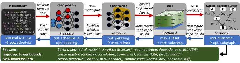
Figure 1. High level overview of the combinatorial SOAP analysis. An input program’s schedule is modeled as the red-blue pebble game. The $X$-Partitioning abstraction relaxes the pebbling problem to the graph partition problem. The SOAP abstraction utilizes the static loop structure to upper-bound the size of the optimal $X$-partition. The Symbolic Directed Graph (SDG) models inter-statement data dependencies. Our method derives I/O lower bounds together with accompanying tile sizes and loop fusions that can be used by a compiler to generate an I/O optimal parallel code.

In our work, we take a different approach based on a combinatorial method. We directly map each elementary computation to a vertex in a parametric CDAG, which allows us not only to operate on unstructured iteration domains, but also to precisely count the sizes of dominator sets and model vertex recomputation. Furthermore, to handle complex data dependencies in programs that evaluate multiple arrays, we introduce the Symbolic Directed Graph (SDG) abstraction, which encapsulates the data flow between elementary computations. This allows us to cover a wider class of programs and handle more complex data flow.

To enable precisely mapping every data access to the parametric CDAG vertex, we introduce a class of Simple Overlap Access Programs (SOAP), and present a general method to derive precise I/O bounds of programs in this class. Specifically, SOAPs are defined as loop nests of statements, whose data access sets can be modeled as injective functions, and their per-statement data overlap can be expressed with constant offsets. For programs that do not directly adhere to SOAP, with nontrivial overlaps and non-injective access functions, we show that under a set of assumptions, we can construct SOAP “projections” of those programs, which can be analyzed in the same way. Our method strictly contains the polyhedral model and associated analysis methods.

To show the breadth of our approach, we demonstrate SOAP analysis on a set of 38 applications, taking Python and C codes as input to create the SDG. This automated analysis procedure generates symbolic bounds, which match or improve upon previously-known results. Notably, we tighten the known I/O lower bounds for numerous programs, including stencils by up to a factor of 14, linear algebra kernels (e.g., Cholesky factorization by a factor of two), and the core convolution operation in deep learning by a factor of 8.

Since our derivation of the bounds is constructive — i.e., it provides loop tilings and fusions after relaxing loop-carried dependencies — the results can be used by a compiler to generate I/O optimal parallel codes. This can both improve existing schedules and possibly reveal new parallelization dimensions.

The paper makes the following contributions:

• A combinatorial method for precisely counting the number of data accesses in parametric CDAGs.

• A class of programs — SOAP — on which I/O lower bounds can be automatically derived.

• Symbolic dataflow analysis that extends SOAP to multiple- statement programs, capturing input and output reuse between statements, as well as data recomputation.

• I/O analysis of 38 scientific computing kernels, improving existing bounds (olivry2020automated, ; chineseCNN1, ) by up to a factor of 14, and new lower bounds for applications in deep learning, unstructured physics simulation, and numerical weather prediction.

2. Background

We first present several fundamental concepts used throughout the paper. We introduce program, memory, and execution models that are based on the work by Hong and Kung (redblue, ). We then present a general approach for deriving I/O lower bounds based on graph partitioning abstractions. The bird’s eye view of our method is presented in Figure 1.

2.1. General Approach of Modeling I/O Costs

Program model: CDAG. One of the most expressive ways to model executions of arbitrary programs is a Computation Directed Acyclic Graph (CDAG) (redblue, ; redblueHierarchy, ; redbluewhite, ; COSMA, ; chineseCNN1, ) $G=(V,E)$, where vertices represent data (either inputs or results of computations) and edges represent data dependencies. That is, for $u,v\in V$, a directed edge $(u,v)\in E$ signifies that $u$ is required to compute $v$. Given vertex $v$, vertices $\{u:(u,v)\in E\}$ are referred to as parents of $v$. Analogously, $\{u:(v,u)\in E\}$ are children of $v$. Vertices with in-degree (out-degree) zero are denoted program inputs (program outputs).

Memory model: red-blue pebble game (redblue, ). Programs are executed on a sequential machine equipped with a two-level memory system, which consists of a fast memory of limited size and unlimited slow memory. The contents of the fast memory are represented by $S$ red pebbles. A red pebble placed on a vertex indicates that the data associated with this vertex resides in the fast memory. Analogously, data residing in the slow memory is represented with blue pebbles (of unlimited number).

Execution model: graph pebbling. An execution of a program represented by a CDAG $G=(V,E)$ is modeled as a sequence of four allowed pebbling moves: 1) placing a red pebble on a vertex which has a blue pebble (load), 2) placing a blue pebble on a vertex which has a red pebble (store), 3) placing a red pebble on a vertex whose parents have red pebbles (compute) 4) removing any pebble from a vertex (discard). At the program start, all input vertices have blue pebbles placed on them. Execution finishes when all output vertices have blue pebbles on them. A sequence of moves leading from the start to the end is called a graph pebbling $P$. The number of load and store moves in $P$ is called the I/O cost of $P$. The I/O cost $Q$ of a program $G$ is the minimum cost among all valid pebbling configurations. A pebbling with cost $Q$ is called optimal.

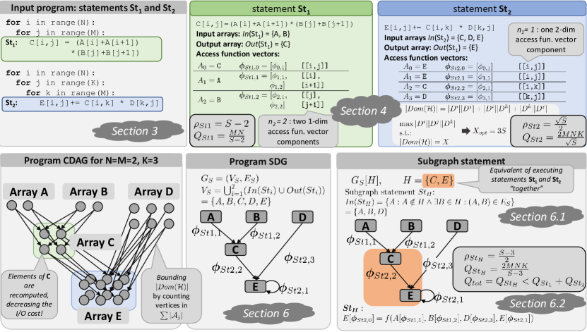
Figure 2. From the input code to the I/O lower bounds. First, for each statement, the access function vectors $\bm{\phi}$ are extracted from the input program (green and blue fields). For each statement, the size of its dominator set is obtained using Lemma 3 (Section 4.2), and then, the I/O lower bound is obtained using inequality 9 (Section 4.5). For programs that contain multiple statements, the SDG is constructed (Section 6) and all valid subgraph statements are evaluated (Section 6.1). Lastly, the final I/O lower bound is obtained (Section 6.2).

2.2. I/O Lower Bounds

Assume that the optimal pebbling $P_{opt}$ is given. For any constant $X>S$ we can partition this sequence of moves into subsequences, such that in each subsequence except of the last one, exactly $X-S$ load/store moves are performed (the last subsequence contains at most $X-S$ load/store moves). Denote the number of these subsequences as $h$. Then observe that $(X-S)(h-1)\leq Q\leq(X-S)h$.

Graph pebbling vs graph partitioning. Since finding $P_{opt}$ is PSPACE complete (redblueHard_, ), we seek to derive a lower bound of $Q$ from the structure of $G$. Observe that the set of vertices which are computed in each subsequence defines a subgraph $\mathcal{H}\subseteq G$. By this construction, computing vertices in $\mathcal{H}$ requires $X-S$ load/store operations in the optimal schedule. The number of subsequences $h$ may be bounded by a particular partitioning of $G$. To do this, we need to introduce two vertex sets defined for any subgraph of $G$.

Dominator and minimum sets (redblue, ). Given $\mathcal{H}\subseteq G$, a dominator set $\mathit{Dom}(\mathcal{H})$ is a set of vertices such that every path from an input to any vertex in $\mathcal{H}$ must contain at least one vertex in $\mathit{Dom}(\mathcal{H})$. The minimum set $\mathit{Min}(\mathcal{H})$ is a set of all vertices in $\mathcal{H}$ that do not have any child in $\mathcal{H}$. To avoid the ambiguity of non-uniqueness of dominator set size, we denote a minimum dominator set $\mathit{Dom}_{min}(\mathcal{H})$ to be a dominator set with the smallest size.

$X$-Partitioning: bounding I/O cost. Introduced by Kwasniewski et al. (COSMA, ), $X$-Partitioning generalizes the S-partitioning from Hong and Kung (redblue, ). Given a constant $X$, an $X$-partition of $G=(V,E)$ is a collection of $s$ mutually disjoint subsets $\mathcal{H}_{i}\subseteq V$ (referred to as subcomputations) $\mathcal{P}(X)=\{\mathcal{H}_{1},\dots,\mathcal{H}_{s}\}:$ $\forall_{i\neq j}\mathcal{H}_{i}\cap\mathcal{H}_{j}=\emptyset\land$ $\bigcup_{i}\mathcal{H}_{i}=V$ with two additional properties:

• there are no cyclic dependencies between subcomputations: $\forall\mathcal{H}_{i}\neq\mathcal{H}_{j}:(\exists(u_{1},v_{1})\in E\text{ s.t. }u_{1}\in\mathcal{H}_{i}\land v_{1}\in\mathcal{H}_{j})\implies(\nexists(v_{2},u_{2})\in E\text{ s.t. }u_{2}\in\mathcal{H}_{i}\land v_{2}\in\mathcal{H}_{j})$

• $\forall\mathcal{H}\in\mathcal{P}(X)$, $\left|{Dom}_{min}\left(\mathcal{H}\right)\right|\leq X$ and $\left|{Min}\left(\mathcal{H}_{h}\right)\right|\leq X$.

The authors prove that for any $X>S$, the optimal pebbling $P_{opt}$ has an associated $X$-partition $\mathcal{P}_{opt}(X)$ s.t. $|\mathcal{P}_{opt}(X)|=h$.

Computational intensity. In previous works it was proven that (a) $Q$ is lower bounded by the number of subsequences $h$ in the optimal pebbling $P_{opt}$ (redblue, ); (b) $h$ is lower bounded by the size of the smallest $X$-partition $|\mathcal{P}_{min}(X)|$ for any value of $X>S$ (COSMA, ); (c) $|\mathcal{P}_{min}(X)|$ is bounded by the maximum size of a single subcomputation $|\mathcal{H}_{X,max}|$ in any valid $X$-partition: $|\mathcal{P}_{min}(X)|\geq{|V|}/{|\mathcal{H}_{X,max}|}$ (COSMA, ); and (d) if $|\mathcal{H}_{X,max}|$ can be expressed as a function of $X$, that is, $\chi(X)\equiv|\mathcal{H}_{X,max}|$, then $Q$ is bounded by

(1) $$Q\geq|V|\frac{X_{0}-S}{\chi(X_{0})},$$

where $X_{0}=\operatorname*{arg\,min}_{X}\frac{\chi(X)}{X-S}$ (Lemma 2 in Kwasniewski et al. (confluxArxiv, )). The expression $\rho=\frac{\chi(X)}{X-S}$ is called the computational intensity.

3. Simple Overlap Access Programs

In Section 2, we show how the I/O cost of a program can be bounded by the maximum size of a subcomputation $\mathcal{H}$ in any valid $X$-partition of program CDAG. We now introduce Simple Overlap Access Programs (SOAP): a class of programs for which we can derive tight analytic bounds of $|\mathcal{H}|$. We leverage the SOAP structure and design an end-to-end method for deriving I/O lower bounds of input programs (summarized in Figure 2).

What is SOAP? Before introducing the formal definition, we start with an illustrative example, which we use in the following sections.

Example 1.

Consider the following 3-point stencil code (we use the Python syntax in code listings):

⬇

for t in range(1,T):

for i in range(t,N-t):

A[i,t+1]=(A[i-1,t] + A[i,t] + A[i+1,t])/3 + B[i]

This is what we will refer to as a single-statement SOAP. The program consists of one statement $St:$ A[i,t+1]=(A[i,t] + ... which is placed in two nested loops. All accessed data comes from static, disjoint, multi-dimensional arrays (A and B). Furthermore, different accesses to the same array (array A is referenced by [i,t+1], [i-1,t], [i,t],[i+1,t]) are offset by a constant stride [0,1], [-1,0],[0,0], [1,0]. We denote such access pattern as a simple overlap and it is a defining property of SOAP.

Why SOAP? We use the restriction on the access pattern to precisely count the number of vertices in $Dom(\mathcal{H})$. If we allow arbitrary overlap of array accesses, we need to conservatively assume a maximum possible overlap of accessed vertices. This reduces the lower bound on $|Dom(\mathcal{H})|$, which, in turn, increases the upper bound on $|\mathcal{H}|$, providing less-tight I/O lower bound for a program.

This is not a fundamental limitation of our method. However, it allows a fully automatic derivation of tight I/O lower bounds for input programs. If the restriction is violated, additional assumptions on the access overlap are needed (Section 5).

SOAP definition. A program is a sequence of statements $St_{1},\dots,St_{k}$. Each such statement $St$ is a constant time computable function $f$ enclosed in a loop nest of the following form:

$$\text{{for }}\psi^{1}\in\mathcal{D}^{1}:$$

$$\dots$$

for $$\psi^{\ell}\in\mathcal{D}^{\ell}(\psi^{1},\dots,\psi^{\ell-1}):$$

$$St:A_{0}[\bm{\phi_{0}}(\bm{\psi})]\leftarrow f(A_{1}[\bm{\phi_{1}}(\bm{\psi})],A_{2}[\bm{\phi_{2}}(\bm{\psi})],\dots,A_{m}[\bm{\phi_{m}}(\bm{\psi})])$$

where:

1. The statement $St$ is nested in a loop nest of depth $\ell$.

2. Each loop in the $t$th level, $t=1,\dots,\ell$ is associated with its iteration variable $\psi^{t}$, which iterates over its domain $\mathcal{D}^{t}\subset\mathbb{N}$. Domain $\mathcal{D}^{t}$ may depend on iteration variables from outer loops $\psi^{1},\dots,\psi^{t-1}$ (denoted as $\mathcal{D}^{t}(\psi^{1},\dots,\psi^{t-1})$).

3. All $\ell$ iteration variables form the iteration vector $\bm{\psi}=[\psi^{1},\dots,\psi^{\ell}]$ and we define the iteration domain $\bm{\mathcal{D}}$ as the set of all values the iteration vector iterates over during the entire execution of the program $\bm{\mathcal{D}}\subset\mathbb{N}^{\ell}$.

4. The dimension of array $A_{j}$ is denoted as $dim(A_{j})$.

5. Elements of $A_{j}$ are referenced by an access function vector $\bm{\phi}_{j}$ which maps $dim(A_{j})$ iteration variables $\bm{\psi}_{j}=[\psi_{j}^{1},\dots,\psi_{j}^{dim(A_{j})}]$ to a set of $\bm{n_{j}}$ elements from $A_{j}$, that is $\bm{\phi}_{j}:\mathcal{D}_{j}^{1}\times,\dots,\times\mathcal{D}_{j}^{dim(A_{j})}$ $\rightarrow$ $\Big{(}\mathbb{N}^{dim(A_{j})}\Big{)}^{n_{j}}$. We then write $\bm{\phi}_{j}=[\bm{\phi}_{j,1},\dots,\bm{\phi}_{j,n_{j}}]$, where $\bm{\phi}_{j,k}:\mathcal{D}_{j}^{1}\times,\dots,\mathcal{D}_{j}^{dim(A_{j})}$ $\rightarrow$ $\mathbb{N}^{dim(A_{j})},k=1,\ \dots,n_{j}$. Furthermore, all access function components $\bm{\phi}_{j,k}(\bm{\psi}_{j})$ are injective.

6. All $n_{j}$ access function vector’s components are equal up to a constant translation vector, that is, $\forall k=1,\dots,n:\bm{\phi}_{j,k}(\bm{\psi})=\bm{\phi}_{j,1}(\bm{\psi})+\bm{t}_{k}$, where $\bm{t}_{k}=[t_{k}^{1},\dots,t_{k}^{dim(A)}]\in\mathbb{N}^{dim(A_{j})}$. We call $\bm{\phi}_{j}$ the simple overlap access.

7. Arrays $A_{1},\dots A_{m}$ are disjoint. If the output array $A_{0}$ is also used as an input, that is, $A_{0}\equiv A_{j},j\geq 1$, then $\bm{\phi}_{0}\cup\bm{\phi}_{j}$ is also the simple overlap access (c.f. Example 1).

8. Each execution of statement $St$ is an evaluation of $f$ for a given value of iteration vector $~{}\bm{\psi}$.

Iteration variables and iteration vectors. Formally, an iteration variable $\psi^{t}$ is an iterator: an object which takes values from its iteration domain during the program execution. However, if it is clear from the context, we will refer to a particular value of the iteration variable simply as $\psi^{t}$ (or a value of iteration vector as $\bm{\psi}$).

Vertices as iteration vectors. Since by definition of CDAG, each computation corresponds to a different vertex, and by definition of SOAP, every statement execution is associated with a single iteration vector $\bm{\psi}$, every non-input vertex in $G$ is uniquely associated with an iteration vector $\bm{\psi}$. Input vertices are referred to by their access function vectors $u=A_{j}[\bm{\phi}_{j,k}(\bm{\psi})]$. We further define CDAG edges as follows: for every value of iteration vector $\bm{\psi}$, we add an edge from all accessed elements to the vertex associated with $\bm{\psi}$, that is: $E=\{(u,v):u=A_{j}[\bm{\phi}_{j,k}(\bm{\psi})],v=\bm{\psi},\bm{\psi}\in\bm{\mathcal{D}}\}$.

$X$-Partitioning on SOAP’s CDAG. Recall that our objective is to bound the maximum size of any subcomputation $|\mathcal{H}|$. Given pebbling $P$ and an associated $X$-partition $\mathcal{P}(X)$, every subcomputation $\mathcal{H}\in\mathcal{P}(X)$ is therefore associated with the set of iteration vectors $\bm{\psi}$ of the vertices computed in $\mathcal{H}$. In the following section we will derive it by counting how many non-input vertices (iteration vectors) can $\mathcal{H}$ contain by bounding its dominator set size $|Dom(\mathcal{H})|$ - again, by counting vertices corresponding to each access $A_{j}[\bm{\phi}_{j,k}(\bm{\psi})]$.

SOAP definition (§ 3)	$A_{0}$	Output array of statement St (may overlap with input arrays).
	$A_{j},$   $j=1,\dots,m$	Mutually disjoint input arrays of statement St.
	$\bm{\psi}=[\psi^{1},\dots,\psi^{\ell}]$	Iteration vector composed of $\ell$ iteration variables.
	$\mathcal{\bm{D}}\subseteq\mathcal{D}^{1}\times,\dots,\times\mathcal{D}^{\ell}$	Iteration domain: a set of values that iteration vector $\bm{\psi}$ takes during the entire program execution.
	$\bm{\phi}_{j}=[\bm{\phi}_{j,1},\dots,\bm{\phi}_{j,n_{j}}]$	Access function vector that maps $dim(A_{j})$ variables $[\psi$ ${}_{j}^{1}$ $,\dots,\psi$ ${}_{j}^{dim(A_{j})}$ $]$ to $n_{j}$ elements in array $A_{j}$.
	$\bm{t}_{j,k}=[t_{j,k}^{1},\dots,t_{j,k}^{dim(A_{j})}]$	Translation vector of $k$-th access function vector’s component $\bm{\phi}_{j,k}$, that is $\bm{\phi}_{j,k}\equiv\bm{\phi}_{j,1},k=1,\dots,n_{j}$
Single-statement subcomputation (§ 4)	$\mathcal{P}(X)=\left\{\mathcal{H}_{1},\dots,\mathcal{H}_{s}\right\}$	An $X$-partition of CDAG $G=(V,E)$ composed of $s$ disjoint subcomputations.
	$\bm{D}=D^{1}\times,\dots,\times D^{\ell}$	Subcomputation domain: a Caresian product of ranges of $\ell$ iteration variables during $\mathcal{H}$.
	$\mathcal{H}\subseteq\bm{D}\subseteq V$	Subcomputation $\mathcal{H}$ uniquely defined by a set of $|\mathcal{H}|$ iteration vector’s values $\bm{\psi}\in\bm{D}$ taken during $\mathcal{H}$. If $\mathcal{H}=\bm{D}$, we call it a rectangular subcomputation $\mathcal{H}_{rec}$.
	$\mathcal{A}=\bm{\phi}[\mathcal{H}]$	Access set: a set of vertices from array $A$ that are accessed by $\bm{\phi}$ during $\mathcal{H}$.
	$\hat{t}^{i}=\{t_{1}^{i},\dots,t_{n}^{i}\}\setminus\{0\}$	Access offset set: set of all non-zero $i$th coordinates among $n$ translation vectors $\bm{t}_{k},k=1,\dots,n$.
	$\mathit{Dom}(\mathcal{H})$	Dominator set of subcomputation $\mathcal{H}$.
	$\rho$	The computational intensity of the $X$-partition.
	$Q\geq|\bm{\mathcal{D}}|\frac{\sum_{j=1}^{m}|\mathcal{A}_{j}(X_{0})|-S}{\prod_{t=1}^{\ell}|D^{t}(X_{0})|}$	A number of I/O operations of a schedule.
SDG (§ 6)	$G_{S}=(V_{S},E_{S})$	Symbolic Directed Graph, where every array accessed in a program is a vertex, and edges represent data dependencies between them.
	$I\subset V_{S}$	Set of read-only arrays of the program.
	$G_{S}[H],H\subset V_{S}\setminus I$	SDG subgraph that represents a subcomputation in which at least one vertex from every array in $H$ is computed.
	$\text{\emph{St}}_{H}$	Subgraph SOAP statement.

Table 1. Notation used in the paper.

4. I/O Lower Bounds For Single-Statement SOAP

We now derive the I/O bounds for programs that contain only one SOAP statement. We start with introducing necessary definitions that allow us to bound the size of a rectangular subcomputation. The summary of the notation is presented in Table 1.

4.1. Definitions

Definition 1.

Subcomputation domain. Denote the set of all values which iteration variable $\psi^{t}$ takes during subcomputation $\mathcal{H}$ as $D^{t}\subset\mathcal{D}^{t},t=1,\dots,\ell$. Then, the subcomputation domain $\bm{D}(\mathcal{H})\subseteq\bm{\mathcal{D}}$ is a Cartesian product of ranges of all $\ell$ iteration variables which they take during $\mathcal{H}$, that is $\bm{D}(\mathcal{H})=D^{1}\times,\dots,\times D^{\ell}$. We therefore have $\mathcal{H}\subseteq\bm{D}(\mathcal{H})\subset\mathbb{N}^{\ell}$. If it is clear from the context, we will sometimes denote $\bm{D}(\mathcal{H})$ simply as $\bm{D}$.

Example 2.

Recall the program from Example 1. Consider subcomputation $\mathcal{H}$ in which $\mathtt{t}\in\{1,2\}$ and $\mathtt{i}\in\{1,2\}$. Then, subcomputation domain $\bm{D}=\{1,2\}\times\{1,2\}=\{[1,1],[1,2],$ $[2,1],[2,2]\}$, but computation itself can contain at most 3 elements $\mathcal{H}\subseteq$ $\{[1,1],[1,2],[2,2]\}$, since $\bm{\psi}=[2,1]\notin\bm{\mathcal{D}}$ does not belong to the iteration domain.

Definition 2.

Access set and access subdomain. Consider input array $A$ and its access function vector $\bm{\phi}$. Given $\mathcal{H}$, the access set $\mathcal{A}$ of $A$ is the set of vertices belonging to $A$ that are accessed during $\mathcal{H}$, that is $\mathcal{A}=\bm{\phi}[\mathcal{H}]=\{A[\bm{\phi}(\bm{\psi})]:\bm{\psi}\in\mathcal{H}\}$. If function $\bm{\phi}=[\bm{\phi}_{1},\dots,\bm{\phi}_{n}]$ accesses $n$ vertices from $A$, we analogously define access sets for each access function component $\bm{\phi}_{k}[\mathcal{H}],k=1,\dots,n$. We then have $\mathcal{A}=\bigcup_{k=1}^{n}\bm{\phi}_{k}[\mathcal{H}]$. The access subdomain $\bm{D}(\mathcal{A})$ is minimum bounding box of the access set $\mathcal{A}$.

Example 3.

For program in Example 1, consider subcomputation $\mathcal{H}$ evaluated on only one iteration vector $\mathcal{H}=[i=2,j=2]$. We have two accessed arrays A and B. Furthermore, we have $\bm{\phi}_{\mathtt{A}}=[[i,t+1],[i-1,t],[i,t],[i-1,t]]$. Therefore, $dim(\mathtt{A})=2$, and $\bm{\phi}_{\mathtt{B}}:\mathbb{N}^{2}\rightarrow\Big{(}\mathbb{N}^{2}\Big{)}^{4}$. We further have $\bm{\phi}_{\mathtt{B}}=[[i]]$, $dim(\mathtt{B})=1$, and $\bm{\phi}_{\mathtt{A}}:\mathbb{N}\rightarrow\mathbb{N}$. To evaluate $St$ for $\bm{\psi}=[2,2]$, we need to access four elements of A (three loads and one store), so its access set is $\mathcal{A}=\bm{\phi}_{\mathtt{A}}[\mathcal{H}]=\{[2,3],[1,2],[2,2],[2,3]\}$. Furthermore, we have the access subdomain $\bm{D}(\mathcal{A})$ $=\{2,3\}\times\{1,2,3\}$.

Definition 3.

Access offset set. Given a simple overlap access $\bm{\phi}=[\bm{\phi}_{1},\dots,\bm{\phi}_{n}]$ consider its $n$ translation vectors $\bm{t}_{k}=[t_{k}^{1},\dots,t_{k}^{dim(A_{j})}]$ $\in\mathbb{N}^{dim(A)},k=1,\dots,n$. For each dimension $i=1,\dots,dim(A_{j})$ we denote $\hat{t}^{i}=\{t_{1}^{i},\dots,t_{n}^{i}\}\setminus\{0\}$ as the set of all unique non-zero $i$th coordinates among all $n$ translation vectors.

Definition 4.

Rectangular subcomputation For a given subcomputation domain $\bm{D}$, a subcomputation $\mathcal{H}$ is called rectangular if $\mathcal{H}=\bm{D}$ and is denoted $\mathcal{H}_{rec}(\bm{D})$. The size of rectangular computation is $|\mathcal{H}_{rec}(\bm{D})|=\prod_{t=1}^{\ell}|D^{t}|$. If it is clear from the context, we will denote $\mathcal{H}_{rec}(\bm{D})$ simply as $\mathcal{H}_{rec}$.

Observation 1.

Consider a simple overlap access $\bm{\phi}=[\bm{\phi}_{1},\dots,\bm{\phi}_{n}]$ of array $A$ and a rectangular subcomputation $\mathcal{H}_{rec}(\bm{D})$. Then since all $\bm{\phi}_{k}$ are equal up to translation, the ranges of iteration variables they access are also equal up to the same translation: $\forall i=1,\dots,dim(A):\forall j=1,\dots,n:\bm{\phi}_{j}[D^{i}]=\bm{\phi}_{1}[D^{i}]+t_{j}$, which also implies that $\forall i=1,\dots,dim(A):\forall j=1,\dots,n:|\bm{\phi}_{j}[D^{i}]|=|\bm{\phi}_{1}[D^{i}]|$.

To bound the sizes of rectangular subcomputations, we use two lemmas given by Kwasniewski et al. (confluxArxiv, ):

Lemma 1.

(Lemma 4 in (confluxArxiv, )) For statement $St$, given $\bm{D}$, the size of subcomputation $\mathcal{H}$ (number of vertices of $S$ computed during $\mathcal{H}$) is bounded by the sizes of the iteration variables’ sets $D^{t},t=1,\dots,\ell$:

(2) $$|\mathcal{H}|\leq\prod_{t=1}^{\ell}|D^{t}|.$$

Proof.

Inequality 2 follows from a combinatorial argument: each computation in $\mathcal{H}$ is uniquely defined by its iteration vector $[\psi^{1},\dots,\psi^{\ell}]$. As each iteration variable $\psi^{t}$ takes $|D^{t}|$ different values during $\mathcal{H}$, we have $|D^{1}|\cdot\dots\cdot|D^{t}|=\prod_{t=1}^{\ell}|D^{t}|$ ways how to uniquely choose the iteration vector in $\mathcal{H}$. ∎

Lemma 2.

(Lemma 5 in (confluxArxiv, )) For the given access function $\bm{\phi}=[\bm{\phi}_{1},\dots,\bm{\phi}_{n}]$ accessing array $A$, $A[\bm{\phi}(\bm{\psi})]$, the access set size of each of components $|\bm{\phi}_{k}[\mathcal{H}]|$ during subcomputation $\mathcal{H}$ is bounded by the sizes of $dim(\bm{\phi}_{A})$ iteration variables’ sets $D^{i},k=1,\dots,dim(\bm{\phi}_{j})$:

(3) $$|\bm{\phi}_{k}[\mathcal{H}]|\leq\prod_{i=1}^{dim(\bm{\phi}_{A})}|D^{i}|$$

where $D^{i}\ni\psi^{i}$ is the iteration domain of variable $\psi^{i}$ during $\mathcal{H}$.

Proof.

We use the same combinatorial argument as in Lemma 1. Since access functions are injective, each vertex in $A$ accessed by $\bm{\phi_{k}}$ is uniquely defined by $[\psi_{k}^{1},\dots,\psi_{k}^{dim(A)}]$. Knowing the number of different values each $\psi_{k}^{j}$ takes in $\mathcal{H}$, we bound the number of different access vectors $\bm{\phi}_{k}[\mathcal{H}]$. ∎

4.2. Bounding SOAP Access Size

Recall that our goal is to find the maximum size of the subcomputation given its dominator size. We first do the converse: given the rectangular subcomputation $\mathcal{H}_{rec}$, we bound the minimum number of input vertices required to compute $\mathcal{H}_{rec}$. In Section 4.4 we prove that indeed $\mathcal{H}_{rec}$ is the subcomputation that upper-bounds the maximum computational intensity $\rho$. Since arrays $A_{1},\dots,A_{m}$ are disjoint, the total number of input vertices is the sum of their access set sizes: $|Dom_{min}(\mathcal{H}_{rec})\geq\sum_{j=1}^{m}|\mathcal{A}_{j}|$. We now proceed to bound individual access set sizes $|\mathcal{A}_{j}|$.

Consider array $A$ with $dim(A)=d$ and its access function $\bm{\phi}(\bm{\psi})=[\bm{\phi}_{1}(\bm{\psi}),\dots,$ $\bm{\phi}_{n}(\bm{\psi})]$ that access $n$ elements from $A$ (to simplify the notation, we drop the subscript $j$, since we consider only one array). Observe that during $\mathcal{H}_{rec}$, all combinations of iteration variables $\psi^{1}\in D^{1},\dots,\psi^{\ell}\in D^{\ell}$ are accessed, so $|\mathcal{H}_{rec}|=\prod_{t=1}^{\ell}|D^{t}|$ (Lemma 1). This also implies that each of $k=1,\dots,n$ accesses to $A$ required $|\bm{\phi}_{k}[\mathcal{H}_{rec}]|=\prod_{t=1}^{d}|D^{t}|$ vertices from $A$ (Lemma 2 and Observation 1). Therefore, the total number of accesses to array $A$ during $\mathcal{H}_{rec}$ is $|\mathcal{A}|\geq\prod_{t=1}^{d}|D^{t}|$. However, the sets of vertices accessed by different $\bm{\phi}_{k}$ may overlap, that is, there may exist two accesses $\bm{\phi}_{l}$ and $\bm{\phi}_{m}$, for which $\bm{\phi}_{l}[\mathcal{H}_{rec}]\cap\bm{\phi}_{m}[\mathcal{H}_{rec}]\neq\emptyset$. Therefore, we also obtain the upper bound $|\mathcal{A}|\leq\sum_{j=1}^{n}\prod_{t=1}^{d}|D^{t}|$. We now want to narrow the gap between the upper and the lower bounds.

Lemma 3.

If a given input array $A$ with $dim(A)=d$ is accessed by a simple overlap access $\bm{\phi}(\bm{\psi})=[\bm{\phi}_{1}(\bm{\psi}),\dots,\bm{\phi}_{n}(\bm{\psi})]$, its access set size $|\mathcal{A}|$ during rectangular computation $\mathcal{H}_{rec}(\bm{D})$ is bounded by

(4) $$|\mathcal{A}|=|\bm{\phi}[\mathcal{H}_{rec}(\bm{D})]|\geq 2\prod_{i=1}^{d}|D^{i}|-\prod_{i=1}^{d}(|D^{i}|-|\hat{t}^{i}|),$$

where $|\hat{t}^{i}|$ is the size of the access offsets set in the $i$th dimension.

Proof.

W.l.o.g., consider the first access function component $\bm{\phi}_{1}$ and its $\prod_{t=1}^{d}|D^{t}|$ accessed vertices $\bm{\phi}_{1}[\mathcal{H}_{rec}]$. We will lower bound the number of accesses to $A$ from remaining $\bm{\phi}_{k},k=2,\dots,n$, which do not overlap with $\bm{\phi}_{1}[\mathcal{H}_{rec}]$, that is $|\bigcup_{k=2}^{n}\bm{\phi}_{k}[\mathcal{H}_{rec}]\setminus\bm{\phi}_{1}[\mathcal{H}_{rec}]|$. Since by construction of $\mathcal{H}_{rec}$, all $\bm{\phi}_{k}[\mathcal{H}_{rec}]$ are Cartesian products of iteration variables’ ranges $\bm{\phi}_{k}[D^{1}]\times,\cdots,$ $\times\bm{\phi}_{k}[D^{d}]$, there is a bijection between $\bm{\phi}_{k}[\mathcal{H}_{rec}]$ and an $d$-dimensional hyperrectangle $H_{k}\in\mathbb{N}^{d}$. To secure correctness of our lower bound on $|\mathcal{A}|$, we need to find the volume of the smallest union of these hyperrectangles.

Note that $|\hat{t}^{i}|$ is a lower bound on the maximum offset between any two $H_{j}\neq H_{k}$ in dimension $i$: the union of all hyperrectangles $\bigcup_{k=1}^{n}H_{k}$ “stretches” at least $|D^{i}|+|\hat{t}^{i}|$ elements in the $i$th dimension for all $i=1,\dots,d$ (see Figure 3). To see this, observe that since $D^{i}\subset N$, for each element in the access offset set $t_{j}^{i}\in\hat{t}^{i}$ there is at least one element in $D^{i}+t_{j}^{i}$ that is not in $D^{i}$, which implies that $|(D^{i}+t_{j}^{i})\setminus D^{i}|\geq 1$. Since $D^{i}$ is finite, there is a single well-defined maximum and a minimum element, which implies that $(\max\{D^{i}\}+t_{j}^{i}\notin D^{i})\lor(\min\{D^{i}\}+t_{j}^{i}\notin D^{i})$. Also, because by definition of $\hat{t}^{i}$ we have $\forall t_{j}^{i},t_{k}^{i}\in\hat{t}^{i}:t_{j}^{i}\neq t_{k}^{i}$, then we also have that each $t_{j}^{i}$ accesses at least one “non-overlapping” element independent of any other $t_{k}^{i}$, that is $\forall t_{j}^{i},t_{k}^{i}\in\hat{t}^{i}:\max\{D^{i}\}+t_{j}^{i}\neq\max\{D^{i}\}+t_{k}^{i}$.

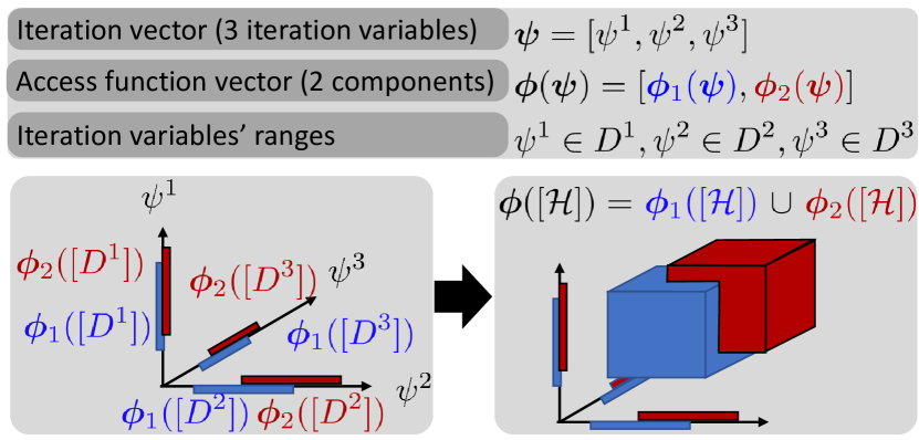
Figure 3. Intuition behind Lemma 3. Access sets $\bm{\phi}_{[}\mathcal{H}_{rec}(\bm{D})]$ as 3-dimensional hyperrectangles. The union $|\bigcup_{k=1}^{n}\bm{\phi}_{k}[\mathcal{H}_{rec}]|$ (and therefore, the total number of accesses $|\mathcal{A}|$ ) is minimized when the hyperrectangles are placed in two antipodal locations of the subcomputation domain $\mathcal{D}$.

The arrangement of hyperrectangles $H_{k},k=1,\dots,n$ in a $\mathbb{N}^{d}$ lattice s.t., their bounding box is $\bm{D}=(|D^{1}|+|\hat{t}^{1}|)\times\dots\times(|D^{d}|+|\hat{t}^{d}|)$, which minimizes the size of their union $|\bigcup_{k}H_{k}|$ satisfies two properties:

1. there exist two “extreme” $H_{p}$, $H_{q}$, such that $H_{q}=H_{p}+\bm{v}$, $\bm{u}=\mathbb{Z}^{d},\forall_{i=1,\dots,d}:|v^{i}|=|\hat{t}^{i}|$,

2. all the remaining $H_{k},k\neq p,q$ perfectly overlap with the “extreme” hyperrectangles $H_{k}\subseteq H_{p}\cup H_{q}$.

To see this, observe that for every non-zero $|\hat{t}^{i}|$ we need two hyperrectangles $H_{p}^{i}\neq H_{q}^{i}$, s.t., $H_{q}^{i}=H_{p}^{i}+[\cdot,\dots,|\hat{t}^{i}|,\dots,\cdot]$, that is, $H_{q}^{i}$ is offset from $H_{p}^{i}$ by $|\hat{t}^{i}|$ in $i$th dimension. We therefore have $\bigcup_{i,|\hat{t}^{i}|>0}(H_{p}^{i}\cup H_{q}^{i})\subseteq\bigcup_{k}H_{k}$. Since $H_{p}^{i}$ and $H_{q}^{i}$ are pairwise non-equal, but there are no restrictions on $H_{p}^{i},H_{p}^{j},i\neq j$, we have that the union $\bigcup_{i,|\hat{t}^{i}|>0}(H_{p}^{i}\cup H_{q}^{i})$ is minimized if $\forall_{i\neq j}H_{p}^{i}=H_{p}^{j}$.

Finally, observe the volume of $|\bigcup_{k=1}^{n}H_{k}|$ s.t. to the claimed arrangement is:

(5) $$\Big{|}\bigcup_{k=1}^{n}H_{k}\Big{|}=|H_{p}\cup H_{q}|=2\prod_{i=1}^{d}|D^{i}|-\prod_{i=1}^{d}(|D^{i}|-|\hat{t}^{i}|)$$

It shows that for any set of $n$ hyperrectangles s.t. the given constraint, the volume of their union is no smaller than the one in Equation 5. Since the offset constraint is also a lower bound on the number of non-overlapping accesses in each dimension, it also forms the bound on $|\bigcup_{k=1}^{n}\bm{\phi}_{k}[\mathcal{H}_{rec}]|=|\bm{\phi}[\mathcal{H}_{rec}]|=|\mathcal{A}|$. ∎

4.3. Input-Output Simple Overlap

If one of the input arrays $A_{i},i\geq 1$, is also the output array $A_{0}$, then their access function vectors $\bm{\phi}_{0}$ and $\bm{\phi}_{i}$ form together a simple overlap access (Section 3). In such cases, some vertices accessed by $\bm{\phi}_{i}$ during $\mathcal{H}_{rec}$ may be computed and do not need to be loaded. We formalize it in the following corollary, which follows directly from Lemma 3:

Corollary 1.

Consider statement $St$ that computes array $A,dim(A)=d$ and simultaneously accesses it as an input $A[\bm{\phi}_{0}(\bm{\psi})]=f(A[\bm{\phi}_{1}(\bm{\psi})])$. If $\bm{\phi}_{0}\cup\bm{\phi}_{1}$ is a simple overlap access, the access set size $|\mathcal{A}|$ during rectangular computation $\mathcal{H}_{rec}$ is bounded by

(6) $$|\mathcal{A}|\geq\prod_{i=1}^{d}|D^{i}|-\prod_{i=1}^{d}(|D^{i}|-|\hat{t}^{i}|),$$

where $\hat{t}$ is an access offset offset set of $\bm{\phi}_{0}\cup\bm{\phi}_{1}$.

Proof.

This result follows directly from Lemma 3. Since there are at least $2\prod_{i=1}^{d}|D^{i}|-\prod_{i=1}^{d}(|D^{i}|-|\hat{t}^{i}|)$ vertices accessed from $A_{i}$, and at most $\prod_{i=1}^{d}|D^{i}|$ of them can be computed during $\mathcal{H}_{rec}$ (Lemma 2) and therefore, do not have to be loaded, then at least $2\prod_{i=1}^{d}|D^{i}|-\prod_{i=1}^{d}(|D^{i}|-|\hat{t}^{i}|)-\prod_{i=1}^{d}|D^{i}|$ elements have to be accessed from the outside of $\mathcal{H}_{rec}$. ∎

4.4. Bounding Maximal Subcomputation

In Section 4.2 we lower-bounded the dominator set size of the rectangular subcomputation $|Dom_{min}(\mathcal{H}_{rec})|=\sum_{j=1}^{m}|\mathcal{A}_{j}|$ by bounding the sizes of simple overlap access sets sizes $|\mathcal{A}_{j}|$ (Lemma 3). Recall that to bound the I/O lower bound we need the size $\chi(X)$ of the maximal subcomputation $\mathcal{H}_{max}$ for given value of $X$ (Inequality 1). We now prove that $\mathcal{H}_{rec}$ upper-bounds the size of $\mathcal{H}_{max}$.

Given $\mathcal{H}$, denote the the ratio of the size of the subcomputation to the dominator set size $\delta(\mathcal{H})=\frac{|\mathcal{H}|}{\sum_{j=1}^{m}|\bm{\phi}_{j}[\mathcal{H}]|}$. By definition, $\mathcal{H}_{max}$ maximizes $\delta$ among all valid $\mathcal{H}\in\mathcal{P}$. We need to show that for a fixed subcomputation domain $\bm{D}_{0}$, among all subcomputations for which $\bm{D}(\mathcal{H})=\bm{D}_{0}$, the rectangular subcomputation $\mathcal{H}_{rec}(\bm{D}_{0})$ upper-bounds $\delta$. Note that an $X$-partition derived from the optimal pebbling schedule $P_{opt}$ may not include $\mathcal{H}_{rec}$. However, $\forall X:\chi_{rec}(X)\geq\chi(X)$, that is, given $X$, the size of $\mathcal{H}_{rec}$ s.t., $\sum_{j=1}^{m}|\bm{\phi}_{j}[\mathcal{H}_{rec}]|=X$ will always be no smaller than the size of $\mathcal{H}_{max}$. To show this, we first need to introduce some auxiliary definitions.

Iteration variables, their indices, and their values. To simplify the notation, throughout the paper we used the iteration variables $\psi^{i}$ and the values they take for some iteration interchangeably. However, now we need to make this distinction explicit. The iteration vector consists of $\ell$ iteration variables $\bm{\psi}=[\psi^{1},\dots,$ $\psi^{\ell}]$. Each access function $\bm{\phi}_{j}$ is defined on $dim(A_{j})$ $\leq\ell$ of them. Recall that $\bm{\psi}_{j}$ is the set of iteration variables accessed by $\bm{\phi}_{j}$ (Section 3, property (5)). To keep track of the indices of particular iteration variables, denote $\bm{\Psi}=[\ell]=\{1,\dots,\ell\}\subset\mathbb{N}$, $\bm{\Psi}_{j}\subseteq\bm{\Psi}$, and $\bm{\Psi}^{\prime}_{j}=\bm{\Psi}\setminus\bm{\Psi}_{j}$ as the sets of integers. If $i\in\bm{\Psi}_{j}$, then the $i$th iteration variable $\psi^{i}$ is accessed by the access function $\bm{\phi}_{j}$. We further define $\bm{\psi}^{*}\in\mathbb{N}^{\ell}$ as a specific value of the iteration vector $\bm{\psi}$ that uniquely defines a single non-input vertex. We analogously define $\bm{\psi}_{j}^{*}$, $\psi^{i,*}$, and $\psi_{j}^{i,*}$ (the last one being a value of $i$th iteration variable of the $j$th access). We also define $\theta(\bm{\psi}_{j}^{*},\mathcal{H})$ as the number of vertices in $\mathcal{H}$ that have all their $\bm{\Psi}_{j}$ coordinates equal to $\bm{\psi}_{j}^{*}$, that is $\theta(\bm{\psi}_{j}^{*},\mathcal{H})=|\{\bm{\psi}^{*}:\bm{\psi}^{*}\in\mathcal{H}\land(\forall i\in\bm{\Psi}_{j}:\psi^{i,*}=\psi_{j}^{i,*})\}|$.

We now formalize our claim in the following lemma:

Lemma 4.

Given the subcomputation domain $\bm{D}_{0}$, $\mathcal{H}_{rec}(\bm{D}_{0})$ maximizes $\delta(\mathcal{H})$ for all $\mathcal{H}$ s.t. $\bm{D}(\mathcal{H})=\bm{D}_{0}$.

(7) $$\forall\mathcal{H}:\delta(\mathcal{H})\leq\delta(\mathcal{H}_{rec})$$

Proof.

Instead of maximizing $\delta(\mathcal{H})$, we will minimize $\delta^{-1}(\mathcal{H})=(\sum_{j=1}^{m}|\bm{\phi}_{j}[\mathcal{H}]|)/|\mathcal{H}|=\sum_{j=1}^{m}|\bm{\phi}_{j}[\mathcal{H}]|/|\mathcal{H}|$ over all possible $\mathcal{H}$. Observe that $\delta^{-1}(\mathcal{H})$ is linear w.r.t. the ratios of individual access function sets sizes $|\bm{\phi}_{j}[\mathcal{H}]|$ and the size of subcomputation $|\mathcal{H}|$. Therefore, we can examine each access $\bm{\phi}_{j}[\mathcal{H}]$ separately and show that every $\delta^{-1}_{j}=|\bm{\phi}_{j}[\mathcal{H}]|/|\mathcal{H}|$ is minimized for $\mathcal{H}=\mathcal{H}_{rec}$. Then, if $\mathcal{H}_{rec}$ minimizes each of $\delta^{-1}_{j}$, then $\delta^{-1}=\sum_{j=1}^{m}\delta^{-1}_{j}$ is minimized, so indeed $\mathcal{H}_{rec}$ maximizes the ratio of the subcomputation size to the dominator set size.

Observe now, that for any $\mathcal{H}$ we have that $\forall_{j}:\delta^{-1}_{j}$ is monotonically decreasing w.r.t. $\theta(\bm{\psi}_{j}^{*},\mathcal{H})$ for all $\bm{\psi}_{j}^{*}\in\bm{\phi}_{j}[\mathcal{H}]$. That is - pick any input vertex $\bm{\psi}_{j}^{*}$ from the set of vertices accessed by $\bm{\phi}_{j}[\mathcal{H}]$. Adding compute vertices $\bm{\psi}^{*}$ to $\mathcal{H}$ that access $\bm{\psi}_{j}^{*}$ do not increase the access set size $\bm{\phi}_{j}[\mathcal{H}]$, since $\bm{\psi}_{j}^{*}$ is already accessed. However, it increases the size of $\mathcal{H}$. Clearly, $\delta^{-1}_{j}$ reaches its minimum if $\forall\bm{\psi}_{j}^{*}\in\bm{\phi}_{j}[\mathcal{H}]:\theta(\bm{\psi}_{j}^{*},\mathcal{H})=\prod_{i\in\bm{\Psi}^{\prime}_{j}}|D^{i}|$, that is, $\mathcal{H}$ computes all vertices spanned by the access set $\bm{\phi}_{j}[\mathcal{H}]$ and all elements in the Cartesian product of “free” (independent of the access function $\phi_{j}$) iteration domains $D^{i},i\in\bm{\Psi}^{\prime}_{j}$.

We showed that for all $j$, given its initial access set $\bm{\phi}_{j}[\mathcal{H}]$, the ratio $\delta^{-1}_{j}$ is minimized for the “almost-rectangular” subcomputation, that is, $\mathcal{H}$ which computes all vertices $\bm{\psi}^{*}\in\bm{\phi}_{j}[\mathcal{H}]\times\prod_{i\in\bm{\Psi}^{\prime}_{j}}D^{i}$. We now need to show that also extending $\mathcal{H}$ over the “dependent” ranges $\bm{\Psi}_{j}$ won’t increase the ratio $\delta^{-1}$. When the access set size $\bm{\phi}_{j}[\mathcal{H}]$ increases by a factor $x$, $\mathcal{H}$ increases proportionally by $x$ too, keeping the ratio constant (See Figure 4 for an example for $\ell=3$).

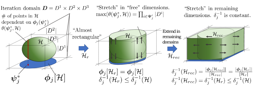
Figure 4. Intuition behind Lemma 4: extending the subcomputation in the free dimensions w.r.t $\bm{\phi}_{j}$ does not increase $|\bm{\phi}_{j}[\mathcal{H}]|$. Once the subcomputation is almost rectangular, extending $H$ in the remaining dimensions keeps the ratio $\delta_{j}^{-1}$ constant.

Since our goal is to minimize each $\delta^{-1}_{j}$ separately, independently of other $\delta^{-1}_{i},i\neq j$, assume that we have already extended $\mathcal{H}$ to the “almost-rectangular” subcomputation, that is, all combinations of $\prod_{i\in\bm{\Psi}^{\prime}_{j}}D^{i}$ were accessed in $\mathcal{H}$. Observe now that $\theta(\bm{\psi}_{j}^{*},\mathcal{H})=\prod_{i\in\bm{\Psi}^{\prime}_{j}}|D^{i}|$ for any vertex $\bm{\psi}_{j}^{*}$. Therefore, since $|\mathcal{H}|=\sum_{\bm{\psi}_{j}^{*}\in\bm{\phi}_{j}[\mathcal{H}]}\prod_{i\in\bm{\Psi}^{\prime}_{j}}|D^{i}|$, we see that $\delta^{-1}_{j}$ is constant w.r.t., the size of the access set: $\delta^{-1}_{j}=\frac{|\bm{\phi}_{j}[\mathcal{H}]|}{|\mathcal{H}|}=\frac{1}{\prod_{i\in\bm{\Psi}^{\prime}_{j}}|D^{i}|}$. Therefore, we can safely maximize $\bm{\phi}_{j}[\mathcal{H}]$ to the entire access set of the rectangular subcomputation $\mathcal{H}_{rec}$ without increasing $\delta_{j}^{-1}$. We conclude that for every access function $\bm{\phi}_{j}$ and every iteration variable index $i$, evaluating all vertices $\bm{\psi}*$ s.t. $\psi^{i}$ iterates over the entire domain $D^{i}$ minimizes $\delta_{j}^{-1}$.

∎

4.5. I/O Lower Bounds and Optimal Tiling

We now proceed to the final step of finding the I/O lower bound. Recall from Section 2.2, that the last missing piece is $\chi(X)$; that is, we seek to express $|\mathcal{H}_{max}(\bm{D})|=\prod_{t=1}^{\ell}|D^{t}|$ as a function of $X$. Observe that by Lemma 4, $|Dom_{min}(\mathcal{H}_{max}(\bm{D}))\geq\sum_{j=1}^{m}(2\prod_{i=1}^{dim(A_{j})}|D_{j}^{i}|-\prod_{i=1}^{dim(A_{j})}(|D_{j}^{i}|-|\hat{t}_{j}^{i}|)$. On the other hand, by definition of $X$-Partitioning, $|Dom_{min}(\mathcal{H}_{max}(\bm{D}))|\leq X$. Combining these inequalities, we solve for all $|D^{t}|$ as functions of $X$ by formulating it as the optimization problem (see Section 3.2 in Kwasniewski et al. (confluxArxiv, )):

$$\max\prod_{t=1}^{\ell}|D^{t}|$$ s.t.

$$\sum_{j=1}^{m}|\mathcal{A}_{j}|\leq X$$

(8) $$\forall 1\geq t\geq\ell:|D^{t}| \geq 1$$

Solving the above optimization problem yields $\chi(X)=|\mathcal{H}_{max}(\bm{D})|$. Since Lemma 4 gives a valid upper bound on computational intensity for any value of $X$, we seek to find the tightest (lowest) upper bound. One can obtain $X_{0}=\operatorname*{arg\,min}_{X}\frac{\chi(X)}{X-S}$, since $\chi(X)$ is differentiable. Finally, combining Lemma 3, inequality 1, and the optimization problem 4.5, we obtain the I/O lower bound for the single-statement SOAP program:

(9) $$Q\geq|\bm{\mathcal{D}}|\frac{\sum_{j=1}^{m}|\mathcal{A}_{j}(X_{0})|-S}{\prod_{t=1}^{\ell}|D^{t}(X_{0})|},$$

where $|\mathcal{A}_{j}(X_{0})|$ are the access set sizes obtained from Lemma 3 for the optimal value of $|D^{i}|$ derived from the optimization problem 4.5.

Substituting $X_{0}$ back to $|D^{t}|(X)$ has a direct interpretation: they constitute optimal loop tilings for the maximal subcomputation. Note that such tiling might be invalid due to problem relaxations: e.g., we ignore loop-carried dependencies and we solve optimization problem 4.5 over real numbers, relaxing the integer constraint on $|D^{t}|$ set sizes. However, this result can serve as a powerful guideline in code generation. Furthermore, if derived tiling sizes generate a valid code, it is provably I/O optimal.

5. Projecting Programs onto SOAP

By the definition of SOAP, one input array may be accessed by different access function vector components, only if they form the simple overlap access — that is, the accesses are offset by a constant stride. However, our analysis may go beyond this constraint if additional assumptions are met.

5.1. Non-Overlapping Access Sets

Given input array $A$ and its access function components $\bm{\phi}(\bm{\psi})=[\bm{\phi}_{1}(\bm{\psi}_{1}),\dots,\bm{\phi}_{n}(\bm{\psi}_{n})]$, if all access sets are disjoint, that is: $\forall_{i\neq j}\bm{\phi}_{i}[\mathcal{D}]\cap\bm{\phi}_{j}[\mathcal{D}]=\emptyset$, then we represent it as $n$ disjoint input arrays $A_{i}$ accessed by single corresponding access function component $\bm{\phi}_{i}(\bm{\psi}_{i})$.

Example 4.

Consider the following code fragment from LU decomposition:

⬇

for k in range(N):

for i in range(k+1,N):

for j in range(k+1,N):

$St:$ A[i,j] = A[i,j] - A[i,k] * A[k,j]

The analysis of iteration variables’ domains $\mathcal{D}^{i},\mathcal{D}^{j},\mathcal{D}^{k}$ shows that for fixed value of $k_{0}$, there are no two iteration vectors $\bm{\psi}_{1}=[k_{0},i_{1},j_{1}]$ and $\bm{\psi}_{2}=[k_{0},i_{2},j_{2}]$ such that $[i_{1},k_{0}]=[k_{0},j_{2}]$ $\lor[i_{1},j_{1}]=[k_{0},j_{2}]$ $\lor[i_{1},j_{1}]=[i_{1},k_{0}]$, therefore, their access sets are disjoint. Furthermore, for $k_{0}$, all elements from $A$ in range $[(k_{0},N),(k_{0},N)]$ are updated. Therefore, all accesses of form $[i_{1},k_{1}]=[k_{2},j_{2}]$ access different vertices. We model this as a SOAP statement with three disjoint arrays:

$$St_{2}:A_{1}[i,j]=f(A_{1}[i,j],A_{2}[i,k],A_{3}[k,j])$$

5.2. Equivalent Input-Output Accesses

If array $A$ is updated by statement $St$ — i.e., it is both input and output — then we require that the output access function $\bm{\phi}_{0}$ is different than the input access function $\bm{\phi}_{i}$. If the input program does not meet this requirement, we can add additional “version dimension” to access functions that is offset by a constant between input and output accesses.

Example 5.

Consider again Example 4. Observe that array $A_{1}$ is updated (it is both the input and the output of $St_{2}$. Furthermore, both access functions are equal: $\bm{\phi}_{0}=\bm{\phi}_{1}=[i,j]$. We can associate a unique version (and therefore, a vertex) of each element of $A$ with a corresponding iteration of the $k$ loop. We add the version dimension associated with $k$ and offset it by constant $1$ between input and output:

$$St_{3}:A_{1}[i,j,k+1]=f(A_{1}[i,j,k],A_{2}[i,k],A_{3}[k,j])$$

5.3. Non-Injective Access Functions

Given input array $A$ and its access function vector $\bm{\phi}$, we require that $\forall\bm{\psi}_{i}\neq\bm{\psi}_{j}:A[\bm{\phi}(\bm{\psi}_{i})]\neq A[\bm{\phi}(\bm{\psi}_{j})]$. If this is not the case, then we seek to bound the size of such overlap, that is, given subcomputation domain $\bm{D}(\mathcal{H})$, how many different iteration vectors $\bm{\psi}_{j}$ map to the same array element $A[\bm{\phi}(\bm{\psi}_{i})]$. We can solve this by analyzing the iteration domain $\bm{\mathcal{D}}$ and the access function vector $\bm{\phi}$. If one array dimension is accessed by a function of multiple iteration variables $g(\phi^{1},\dots,\phi^{k})$ and $g$ is linear w.r.t. all $\phi^{i}$, the number of different values $g$ takes in $\bm{D}(\mathcal{H})$ is bounded by $\max_{i=1,\dots,k}\{|D^{i}|\}\leq|g[\mathcal{H}]|\leq\prod_{i=1}^{k}|D^{i}|$, for $D^{i}\neq\{0\},i=1,\dots,k$.

Example 6.

A single layer of the direct convolution used in neural networks may be written as seven nested loops with iteration variables $b,c,k,w,h,r,s$ and statement (c.f. (demmelCNN, )):

$$St:Out[k,h,w,b]+=Image[r+\sigma_{w}w,s+\sigma_{h}h,c,b]\times Filter[k,r,s]$$

Depending on the value of $\sigma_{w}$ and $\sigma_{h}$, the access function of $Image$, $\bm{\phi}=[r+\sigma_{w}w,s+\sigma_{h}h,c,b]$ may not be injective. Yet, observe that:

1. $\sigma_{w}\geq|D^{r}|\land\sigma_{h}\geq|D^{s}|\implies\bm{\phi}$ is injective $\implies$ $|\bm{\phi}[\mathcal{H}_{max}]|\geq|D^{r}|\cdot|D^{w}|\cdot|D^{s}|\cdot|D^{h}|\cdot|D^{c}|\cdot|D^{b}|$

2. $\sigma_{w}=1\land\sigma_{h}=1\implies|\bm{\phi}[\mathcal{H}_{max}]|\geq$ $\max(|D^{r}|,|D^{w}|)\cdot\max(|D^{s}|,|D^{h}|)\cdot|D^{c}|\cdot|D^{b}|$,

Our analysis provides a conditional computational intensity: $\rho_{min}=\sqrt{S}/2$ in case (1) and $\rho_{max}=S/2$ in case (2). Observe that case (2) yields the maximum non-injective overlap (maximum number of different iteration vectors map to the same element in $Image$). For any other values of $\sigma_{w}$ and $\sigma_{h}$, we have $\rho_{min}\leq\rho\leq\rho_{max}$.

6. Multi-Statement SOAP

I/O lower bounds are not composable: the I/O cost of a program containing multiple statements may be lower than the sum of the I/O costs of each statement if evaluated in isolation. Data may be reused and merging of statements may lower the I/O cost.

Note that the number of vertices in the program’s CDAG $G$ depend on domain sizes $D^{i}$ of each iteration variable. However, our derived upper bound of the computational intensity $\rho$ is independent of the CDAG size, as it depends only on the access functions $\bm{\phi}_{j}$. This is also true for programs that contain multiple statements - to bound $\rho$ for multi-statement SOAP, we only need to model dependencies between the arrays and how they are accessed - e.g., one statement may take as an input an array that is an output of a different statement.

We represent the data flow between the program statements with a symbolic directed graph $G_{S}=(V_{S},E_{S})$. For a given statement $St_{i}$, denote $In(St_{i})=\{A_{i,1},\dots,A_{i,m}\}$ a set of input arrays of statement $St_{i}$. Analogously, denote $Out(St_{i})$ the set containing the output array of $St_{i}$. Analogously to program CDAG $G$ that captured dependencies between particular array elements, $G_{S}$ models dependencies between whole arrays (Figure 2).

Definition 5.

Symbolic Digraph: SDG Given $k$-statement SOAP ${St_{1},\dots,St_{k}}$, its symbolic digraph (SDG) $G_{S}=(V_{S},E_{S})$ is a directed graph where $V_{S}=\bigcup_{i=1}^{k}(\text{In}(St_{i})\cup\text{Out}(St_{i}))$ and $(A_{u},A_{v})\in E_{S}\iff\exists St_{i}:A_{u}\in In(St_{i})\land A_{v}\in Out(St_{i})$.

$G_{S}$ is a directed graph, where vertices represent arrays accessed by a program, and edges represent data dependencies between them. Two arrays $A_{u}$ and $A_{v}$ are connected if there is a statement that accesses $A_{u}$ and computes $A_{v}$. Each edge is annotated with the corresponding access function vector of the statement that generates it.

Example 7.

Consider the example in Figure 2. We have two statements $St_{1}$ and $St_{2}$, with $\text{In}(St_{1})=\{A,B\}$, $\text{Out}(St_{1})=\{C\}$, $\text{In}(St_{2})=\{C,D,E\}$, $\text{Out}(St_{2})=\{E\}$. We then construct the SDG $G_{S}=(V_{S},E_{S})$, with $V_{S}=\text{In}(St_{1})\cup\text{Out}(St_{1})\cup\text{In}(St_{2})\cup\text{Out}(St_{2})=\{A,B,C,D,E\}$. Furthermore, we have edges $E_{S}=\{(A,C),(B,C),(C,E),(D,E),(E,E)\}$. The edges are annotated with the corresponding access function vectors $\bm{\phi}_{St1,1},\dots,\bm{\phi}_{St2,3}$.

Note: While the “explicit” program CDAG $G=(V,E)$, where every vertex represents a single computation is indeed acyclic, the SDG $G_{S}=(V_{S},E_{S})$ may contain self-edges when a statement updates the loaded array ($(E,E)$ in the example above). In $G$, one vertex corresponds to one version of a single array element, while in $G_{S}$, one vertex encapsulates all versions of all array elements.

6.1. SDG Subgraphs

Denote $I\subset V_{S}$ set of input vertices of $G_{S}$ ($\forall A\in I:\text{indegree}(A)=0$). Let $H\subset V_{S}\setminus I$ be a subset of the vertices of SDG $G_{S}=(V_{S},E_{S})$. The SDG subgraph $G_{S}[H]$ is a subgraph of $G_{S}$ induced by the vertex set $H$. It corresponds to some subcomputation in which at least one vertex from each array in $H$ was computed. We now use the analogous strategy to the $X$-Partitioning abstraction: since the optimal pebbling has an associated $X$-partition with certain properties (the dominator set constraint), we bound the cost of any pebbling by finding the maximum subcomputation among all valid $X$-partitions. We now show that every subcomputation in the optimal $X$-partition has a corresponding SDG subgraph $G_{S}[H]$. Therefore, finding $G_{S}[H_{opt}]$ that maximizes the computational intensity among all subgraphs bounds the size of the maximal subcomputation (which, in turn, bounds the I/O cost of any pebbling).

Recall that an optimal pebbling $P$ has an associated $X$-partition $\mathcal{P}(X)$, where each $\mathcal{H}\in\mathcal{P}(X)$ represents a sequence of operations that are not interleaved with other subcomputations. Given $G_{S}$, each $\mathcal{H}\in\mathcal{P}(X)$ has an associated subgraph $G_{S}[H]$ s.t. every array vertex $A_{i}\in H$ represents an array from which at least one vertex was computed in $\mathcal{H}$.

Note that both the pebbling $P$ and the partition $\mathcal{P}(X)$ depend on the size of the CDAG that is determined by the sizes of the iteration domains $D^{i}$. However, the SDG does not depend on them. Thus, by finding the subgraph that maximizes the computational intensity, we bound $\rho$ for any combination of input parameters.

Definition 6.

The subgraph SOAP statement $St_{H}$ of subgraph $G_{S}[H]$ is a single SOAP statement with the input $In(St_{H})=\{A:A\notin H\land\exists B\in H:(A,B)\in E_{S}\}$. Additionally, for each vertex $B\in H$ that is not computed in $H$, that is $\nexists A\in H:(A,B)\in E_{S}$ , self-edges $(B,B)\in E$ are preserved ($B\in In(St_{H})$).

Intuition. The subgraph statement $St_{H}$ is a “virtual” SOAP statement that encapsulates multiple statements $St_{1},\dots,St_{k}$. Given $H$, its subgraph statement’s inputs $In(St_{H})$ are formed by merging inputs $\bigcup_{i=1}^{k}In(St_{i})\setminus V(H)$ from all statements that form $H$, but are not in $H$. By the construction of the SDG, this is equivalent to the definition above: take all vertices $A\in V_{s}\setminus V(H)$ that have a child in $V(H)$, that is $\exists B\in V(H):(A,B)\in E_{S}$ (see Figure 2).

This forms the lower bound on the number of inputs for a corresponding subcomputation $\mathcal{H}$: all the vertices from arrays $A_{i}\in V(H)$ could potentially be computed during $\mathcal{H}$ and do not need to be loaded, but at least vertices from arrays $In(St_{H})$ have to be accessed.

Example 8.

Consider again the example from Figure 2. The set of input nodes is $I=\{A,B,D\}$. There are three possible subgraph statements: $H_{1}=\{C\}$, with $In(St_{H_{1}})=\{A,B\}$, $H_{2}=\{C\}$ with $In(St_{H_{2}})=\{C,D,E\}$, and $H_{3}=\{C,E\}$ with $In(St_{H_{3}})=\{A,B,D\}$. Note that by definition, the self-edge $(C,C)$ is preserved in $H_{2}$, but not in $H_{3}$. Subgraphs $H_{1}$ and $H_{2}$ correspond to the input statements $St_{1}$ and $St_{2}$. Subgraph $H_{3}$ encapsulates a subcomputation $\mathcal{H}$ that computes some vertices from both arrays $C$ and $E$, merging subcomputations $St_{1}$ and $St_{2}$ and reusing outputs from $St_{1}$ to compute $E$.

Then, we establish the following lemma:

Lemma 5.

Given an $X$-partition $\mathcal{P}(X)=\{\mathcal{H}_{1},\dots,\mathcal{H}_{s}\}$ of the $k$-statement SOAP, with its corresponding $G_{S}=(V_{S},E_{S})$, each subcomputation $\mathcal{H}$ has an associated intensity $\rho_{\mathcal{H}}=\frac{|\mathcal{H}|}{|Dom_{min}(\mathcal{H})|-S}$ that is upper-bounded by the computational intensity of the subgraph statement $St_{H}$ (Lemma 4).

Proof.

Recall that given the subcomputation $\mathcal{H}$, its corresponding SDG subgraph $H$ is constructed as follows: for each vertex $v\in V$ computed during $\mathcal{H}$ belonging to some array $A_{i}$, add the corresponding array vertex $s_{i}$ to $H$. Note that we allow a vertex recomputation: if some vertex is (re)computed during the optimal schedule of $\mathcal{H}$, its array vertex will belong to $H$.

Observe that by this construction and by definition of the subgraph statement, all arrays from which at least one vertex is loaded during $\mathcal{H}$ are in $In(St_{H})$. Furthermore, $In(St_{H})$ is a subset of these arrays: during $\mathcal{H}$, there might be some loaded vertex from array $A_{j}\in H$, but, by definition of $St_{H}$, this array will not be in $In(St_{H})$. Therefore, $St_{H}$ lower bounds the input size of $\mathcal{H}$.

The last step of the proof is to observe that by Lemma 4, the computational intensity of $St_{H}$ bounds the maximum number of computed vertices for any $\mathcal{H}^{\prime}\in\mathcal{P}(X)$ that belong to $H$, that is, the union of all arrays in $H$. But since all vertices that are computed in $\mathcal{H}$ belong to one of these arrays, $\mathcal{H}$ cannot have higher computational intensity. ∎

6.2. SDG I/O Lower Bounds

We now proceed to establish a method to derive the I/O lower bounds of the multi-statement SOAP given its SDG $G_{S}=(V_{S},E_{S})$.

For each array vertex $A\in V_{S}$, denote $|A|$ as the total number of vertices in the CDAG that belong to array $A$. Denote further $\mathcal{S}(A)$ the set of all subgraphs of $G_{S}$ that contain $A$. Then we prove the following theorem:

Theorem 1.

The I/O cost $Q$ of a $k$-statement SOAP represented by the SDG $G_{S}=(V_{S},E_{S})$ is bounded by

(10) $$Q\geq\sum_{A\in V_{S}}\frac{|A|}{\max_{H\in\mathcal{S}(A)}\rho_{H}}$$

where $\max_{H\in\mathcal{S}(A)}\rho_{H}$ is the maximum computational intensity over all subgraph statements of subgraphs $H$ that contain vertex $A$.

Proof.

This theorem is a direct consequence of Lemma 5 and the fact that all vertices in CDAG $G$ are associated with some array vertex in SDG $G_{S}$. Lemma 5, together with the definition of $\mathcal{S}(a)$, states that $\max_{H\in\mathcal{S}(a)}\rho_{H}$ is the upper bound on any subcomputation $\mathcal{H}$ that contains any vertex from array $a$. Since there are $|a|$ vertices associated with $a$, at least $\frac{|a|}{\max_{H\in\mathcal{S}(a)}\rho_{H}}$ I/O operations must be performed to compute these vertices. Since the computational intensity expresses the average cost per vertex, even if some subcomputation in an optimal $X$-partition spans more than one array, this is already modeled by the set $\mathcal{S}(a)$. Therefore, we can sum the I/O costs per arrays $a$, yielding inequality 10. ∎

Note that applying Theorem 1 requires iterating over all possible subgraphs. In the worst case, this yields exponential complexity, prohibiting scaling our method to large programs. However, many scientific applications contain a limited number of kernels with simple dependencies. In practice we observed that our approach scales well to programs containing up to 35 statements.

7. Evaluation

We evaluate our lower bound analysis on a wide range of applications, ranging from fundamental computational kernels and solvers to full workloads in hydrodynamics, numerical weather prediction, and deep learning. The set of applications covers both the previously analyzed kernels (the Polybench suite (polybench, ), direct convolution), and kernels that were never analyzed before due to complicated dependency structures (multiple NN layers, diffusion, advection). Not only our tool covers broader class of programs than state-of-the-art approaches, but also it improves bounds generated by methods dedicated to specific narrower classes (olivry2020automated, ). Improving I/O lower bounds has not only theoretical implications: loose bounds may not be applicable for generating corresponding parallel codes, as too many overapproximations may yield an invalid schedule.

In our experiments we use DaCe (dace, ) to extract SOAP statements from Python and C code, and use MATLAB for symbolic analysis.

			Improv.
	Kernel	SOAP I/O Bound	over SotA
Polybench(olivry2020automated, )	adi	$\frac{12N^{2}T}{\sqrt{S}}$	$\frac{12}{\sqrt{S}}$
	atax	$MN$	$1$
	bicg	$MN$	$1$
	cholesky	$\frac{N^{3}}{3\sqrt{S}}$	$2$
	correlation	$\frac{M^{2}N}{\sqrt{S}}$	$2$
	covariance	$\frac{M^{2}N}{\sqrt{S}}$	$2$
	deriche	$3HW$	$3$
	doitgen	$\frac{2N_{P}^{2}N_{Q}N_{R}}{\sqrt{S}}$	$1$
	durbin	$\frac{3N^{2}}{2}$	$3$
	fdtd2d	$\frac{2\sqrt{3}N_{X}N_{Y}T}{\sqrt{S}}$	$6\sqrt{6}$
	floyd-warshall	$\frac{2N^{3}}{\sqrt{S}}$	$2$
	gemm	$\frac{2N^{2}}{\sqrt{S}}$	$1$
	gemver	$N^{2}$	$1$
	gesummv	$2N^{2}$	$1$
	gramschmidt	$\frac{MN^{2}}{\sqrt{S}}$	$1$
	heat3d	$\frac{6N^{3}T}{\sqrt[3]{S}}$	$\frac{32}{3\sqrt[3]{3}}$
	jacobi1d	$\frac{2NT}{S}$	$8$
	jacobi2d	$\frac{4N^{2}T}{\sqrt{S}}$	$6\sqrt{3}$
	2mm	$\frac{4N^{3}}{\sqrt{S}}$	$1$
	3mm	$\frac{6N^{3}}{\sqrt{S}}$	$1$
	lu	$\frac{2N^{3}}{3\sqrt{S}}$	$1$
	ludcmp	$\frac{2N^{3}}{3\sqrt{S}}$	$1$
	mvt	$N^{2}$	$1$
	nussinov	$\frac{N^{3}}{3\sqrt{S}}$	$2$
	seidel2d	$\frac{4N^{2}T}{\sqrt{S}}$	$6\sqrt{3}$
	symm	$\frac{2M^{2}N}{\sqrt{S}}$	$1$
	syr2k	$\frac{2MN^{2}}{\sqrt{S}}$	$2$
	syrk	$\frac{MN^{2}}{\sqrt{S}}$	$2$
	trisolv	$\frac{N^{2}}{2}$	$1$
	trmm	$\frac{M^{2}N}{\sqrt{S}}$	$1$
Neural Networks	Direct conv.	$\frac{2C_{in}C_{out}H_{out}NW_{out}W_{ker}H_{ker}}{\sqrt{S}}$	8
	Softmax	$4BHMN$	—
	MLP	$\frac{2N(fc_{1}fc_{2}+fc_{1}inp+fc_{2}out)}{\sqrt{S}}$	—
	LeNet-5	$\frac{300\sqrt{2}CHNW}{\sqrt{S}}$	—
	BERT Encoder	$\frac{4\,B\,H\,P\,L\,\left(L+2\,H\,P\right)}{\sqrt{S}}$	—
Various	LULESH	$22\cdot\text{numElem}$	—
	horizontal diff.	$2IJK$	—
	vertical adv.	$5IJK$	—

Table 2. Simplified leading-order terms of the I/O lower bounds extracted from multi-statement SOAP and previous state-of-the-art. For the direct convolution layer, the best previously known bound was published by Zhang et al. (chineseCNN1, ).

Polybench. As our first case study, we analyze Polybench (polybench, ), a polyhedral application benchmark suite composed of 30 programs from several domains, including linear algebra kernels, linear solvers, data mining, and computational biology. Prior best results were obtained by IOLB (olivry2020automated, ), a tool specifically designed for analyzing I/O lower bounds of affine programs. We summarize the results in Table 2, listing the leading order term for brevity.

We find that SOAP analysis derives tight I/O lower bounds for all Polybench kernels. Analyzing these programs as multi-statement SOAP either reproduces existing tight bounds, or improves them by constant factors (e.g., in Cholesky decomposition) on 14 out of 30 applications (Table 2). Of particular note is adi (Alternating Direction Implicit solver). Our algorithm detected a possible tiling in the time dimension, yielding the lower bound $(12N^{2}T)/\sqrt{S}$, compared to $N^{2}T$ reported by Olivry et al. (olivry2020automated, ). However, due to dependency chains incurred by alternating directions, such tiling may violate loop-carried dependency constraints, which our algorithm relaxes. A parallel machine could potentially take advantage of this tiling scheme, possibly providing super-linear communication reduction. However, this is outside of the scope of this paper.

Neural Networks. Analyzing I/O lower bounds of neural networks is a nascent field, and so far only single-layer convolution was analyzed (demmelCNN, ; chineseCNN1, ). We improve the previously-reported bound reported by Zhang et al. (chineseCNN1, ) by a factor of 8.

7.1. New Lower Bounds

Analyzing SOAP and the SDG representation enables capturing complex data dependencies in programs with a large number of statements. To demonstrate this, we study larger programs in three fields, where no previous I/O bounds are known. If an application contains both SOAP and data-dependent kernels, we find a SOAP representation that bounds the access sizes from below.

LULESH. The Livermore Unstructured Lagrangian Explicit Shock Hydrodynamics (LULESH) (lulesh, ) application is an unstructured phy-sics simulation. We analyze the main computational kernel, totaling over 60% of runtime within one time-step of the simulation from the full C++ source code. As LULESH falls outside the purview of affine programs, this result is the first reported I/O lower bound.

Numerical Weather Prediction. We select two benchmark stencil applications from the COSMO Weather Model (cosmo, ) — horizontal diffusion and vertical advection — representatives of the two major workload types in the model’s dynamical core.

Deep Neural Networks. For deep learning, we choose both individual representative operators (Convolution and Softmax) and network-scale benchmarks. Previous approaches only study data movement empirically (ivanov20, ). To the best of our knowledge, we are the first to obtain I/O lower bounds for full networks, including a Multi-Layer Perceptron (MLP), the LeNet-5 CNN (lenet, ), and a BERT Transformer encoder (transformer, ).

8. Related Work

I/O analysis spans almost the entire history of general-purpose computer architectures, and graph pebbling abstractions were among the first methods to model memory requirements. Dating back to challenges with the register allocation problem (completeRegisterProblems, ), pebbles were also used to prove space-time tradeoffs (pebbleTradeoffs, ) and maximum parallel speedups by investigating circuit depths (dymond1985speedups, ). Arguably the most influential pebbling abstraction work is the red-blue pebble game by Hong and Kung (redblue, ) that explicitly models load and store operations in a two-level-deep memory hierarchy. This work was extended numerous times, by: adding blocked access (externalMem, ), multiple memory hierarchies (redblueHierarchy, ), or introducing additional pebbles to allow CDAG compositions (redbluewhite, ). Demaine and Liu proved that finding the optimal pebbling in a standard and no-deletion red-blue pebble game is PSPACE-complete (redbluehardSPAA, ). Papp and Wattenhofer introduced a game variant with a non-zero computation cost and investigated pebbling approximation algorithms (papp2020hardness, ).

Although the importance of data movement minimization is beyond doubt, the general solution for arbitrary algorithms is still an open problem. Therefore, many works were dedicated to investigate lower bounds only for single algorithms (often with accompanying implementations), like matrix-matrix multiplication (loomisApplied, ; 2.5DLU, ; CARMA, ; COSMA, ), LU (2.5DLU, ) and Cholesky decompositions (cholesky1, ; choleskyQRnew, ). Ballard et al. (ballard2014communication, ) present an extensive collection of linear algebra algorithms. Moreover, a large body of work exists for minimizing communication in irregular algorithms (besta2015accelerating, ; sakr2020future, ), such as Betweenness Centrality (maciejBC, ), min cuts (gianinazzi2018communication, ), BFS (slimsell, ), matchings (besta2020substream, ), vertex similarity coefficients (besta2020communication, ), or general graph computations (besta2017push, ; besta2021graphminesuite, ; besta2021graphminesuite, ). Many of them use linear algebra based formulations (kepner2016mathematical, ). Recently, convolution networks gained high attention. The first asymptotic I/O lower bound for single-layer direct convolution was proved by Demmel et al. (demmelCNN, ). Chen et al. (chineseCNN2, ) propose a matching implementation, and Zhang et al. (chineseCNN1, ) present the first non-asymptotic I/O lower bound for Winograd convolution.

In parallel with the development of I/O minimizing implementations for particular algorithms, several works investigated I/O lower bounds for whole classes of programs. Christ et al. (general_arrays, ) use a discrete version of Loomis-Whitney inequality to derive asymptotic lower bounds for single-statement programs nested in affine loops. Demmel and Rusciano (demmelHBL, ) extended this work and use discrete Hölder-Brascamp-Lieb inequalities to find optimal tilings for such programs. The polyhedral model (polyhedralModel, ) is widely used in practice by many compilers (pluto, ; polly, ). However, polyhedral methods have their own limitations: 1) they cannot capture non-affine loops (loopcounting, ); 2) while the representation of a program is polynomial, finding optimal transformations is still NP-hard (loopFusionComplexity, ); 3) they are inapplicable for many neural network architectures, e.g., the Winograd algorithm for convolution (chineseCNN1, ).

Recently, Olivry et al. (olivry2020automated, ) presented IOLB — a tool for automatic derivation of non-parametric I/O lower bounds for programs that can be modeled by the polyhedral framework. IOLB employs both “geometric” projection-based bounds based on the HBL inequality (demmel1, ), as well as the wavefront-based approach from Elango (elango2014characterizing, ). To the best of our knowledge, this is the only method that can handle multiple-statement programs. However, the IOLB model explicitly disallows recomputation that may be used to decrease the I/O cost, e.g., in the Winograd convolution algorithm, backpropagation, or vertical advection. Furthermore, the framework is strictly limited to affine access programs. Even then, our method is able to improve those bounds by up to a factor of $6\sqrt{6}$ (fdtd2d) using a single, general method without the need to use application-specific techniques, such as wavefront-based reasoning.

9. Conclusions

In this work we introduce SOAP — a broad class of statically analyzable programs. Using the explicit assumptions on the allowed overlap between arrays, we are able to precisely count the number of accessed vertices on the induced parametric CDAG. This stands in contrast with many state-of-the art approaches that are based on bounding projection sizes, as they need to underapproximate their union size, often resulting in a significant slack in constant factors of their bounds. Our single method is able to reproduce or improve existing lower bounds for many important scientific kernels from various domains, ranging from 2$\times$ increase in the lower bound for linear algebra (cholesky, syrk), to more than 10$\times$ for stencil applications (fdtd2d, heat3d).

Our SDG abstraction precisely models data dependencies in multiple-statement programs. It directly captures input and output reuse, and allows data recomputation. Armed with these tools, we are the first to establish I/O lower bounds for entire neural networks, as well as core components of the popular Transformer architecture.

We believe that our work will be further extended to handle data-dependent accesses (e.g., sparse matrices), as well as scale better with input program size. The derived maximum subcomputation sizes can guide compiler optimizations and development of new communication-optimal algorithms through tiling, parallelization, or loop fusion transformations.

10. Acknowledgements

This project received funding from the European Research Council (ERC) under the European Union’s Horizon 2020 programme (grant agreement DAPP, No. 678880). Tal Ben-Nun is supported by the Swiss National Science Foundation (Ambizione Project #185778). The authors wish to thank the Swiss National Supercomputing Center (CSCS) for providing computing infrastructure and support.

References

- (1) D. Unat, A. Dubey, T. Hoefler, J. Shalf, M. Abraham, M. Bianco, B. L. Chamberlain, R. Cledat, H. C. Edwards, H. Finkel, K. Fuerlinger, F. Hannig, E. Jeannot, A. Kamil, J. Keasler, P. H. J. Kelly, V. Leung, H. Ltaief, N. Maruyama, C. J. Newburn, , and M. Pericas, “Trends in Data Locality Abstractions for HPC Systems,” IEEE Transactions on Parallel and Distributed Systems (TPDS), vol. 28, no. 10, Oct. 2017.
- (2) G. Kestor, R. Gioiosa, D. J. Kerbyson, and A. Hoisie, “Quantifying the energy cost of data movement in scientific applications,” in 2013 IEEE international symposium on workload characterization (IISWC). IEEE, 2013, pp. 56–65.
- (3) A. Tate, A. Kamil, A. Dubey, A. Größlinger, B. Chamberlain, B. Goglin, C. Edwards, C. J. Newburn, D. Padua, D. Unat et al., “Programming abstractions for data locality.” PADAL Workshop 2014.
- (4) D. Unat, A. Dubey, T. Hoefler, J. Shalf, M. Abraham, M. Bianco, B. L. Chamberlain, R. Cledat, H. C. Edwards, H. Finkel, K. Fuerlinger, F. Hannig, E. Jeannot, A. Kamil, J. Keasler, P. H. J. Kelly, V. Leung, H. Ltaief, N. Maruyama, C. J. Newburn, and M. Pericás, “Trends in data locality abstractions for hpc systems,” IEEE Transactions on Parallel and Distributed Systems, pp. 3007–3020, 2017.
- (5) E. Solomonik, M. Besta, F. Vella, and T. Hoefler, “Scaling Betweenness Centrality using Communication-Efficient Sparse Matrix Multiplication,” in SC, 2017.
- (6) E. Solomonik, E. Carson, N. Knight, and J. Demmel, “Trade-offs between synchronization, communication, and computation in parallel linear algebra computations,” ACM Transactions on Parallel Computing (TOPC), vol. 3, no. 1, pp. 1–47, 2017.
- (7) M. Christ, J. Demmel, N. Knight, T. Scanlon, and K. Yelick, “Communication lower bounds and optimal algorithms for programs that reference arrays–part 1,” arXiv preprint arXiv:1308.0068, 2013.
- (8) J. Hong and H. Kung, “I/O complexity: The red-blue pebble game,” in STOC, 1981, pp. 326–333.
- (9) M. Del Ben et al., “Enabling simulation at the fifth rung of DFT: Large scale RPA calculations with excellent time to solution,” Comp. Phys. Comm., pp. 120–129, 2015.
- (10) Q. Zheng and J. D. Lafferty, “Convergence analysis for rectangular matrix completion using burer-monteiro factorization and gradient descent,” CoRR, 2016.
- (11) T. Ben-Nun and T. Hoefler, “Demystifying parallel and distributed deep learning: An in-depth concurrency analysis,” ACM Comput. Surv., vol. 52, no. 4, 2019.
- (12) C. D. Meyer, Matrix analysis and applied linear algebra. SIAM, 2000.
- (13) A. Krishnamoorthy and D. Menon, “Matrix inversion using Cholesky decomposition,” in 2013 signal processing: Algorithms, architectures, arrangements, and applications (SPA). IEEE, 2013, pp. 70–72.
- (14) E. Solomonik, D. Matthews, J. R. Hammond, J. F. Stanton, and J. Demmel, “A massively parallel tensor contraction framework for coupled-cluster computations,” Journal of Parallel and Distributed Computing, vol. 74, no. 12, pp. 3176–3190, 2014.
- (15) V. Elango, F. Rastello, L.-N. Pouchet, J. Ramanujam, and P. Sadayappan, “On characterizing the data access complexity of programs,” in Proceedings of the 42Nd Annual ACM SIGPLAN-SIGACT Symposium on Principles of Programming Languages, ser. POPL ’15. New York, NY, USA: ACM, 2015.
- (16) G. Kwasniewski, M. Kabić, M. Besta, J. VandeVondele, R. Solcà, and T. Hoefler, “Red-Blue Pebbling Revisited: Near Optimal Parallel Matrix-Matrix Multiplication,” in Proceedings of the International Conference for High Performance Computing, Networking, Storage and Analysis (SC19), Nov. 2019.
- (17) E. D. Demaine and Q. C. Liu, “Red-blue pebble game: Complexity of computing the trade-off between cache size and memory transfers,” in Proceedings of the 30th on Symposium on Parallelism in Algorithms and Architectures, 2018, pp. 195–204.
- (18) V. Elango et al., “Data access complexity: The red/blue pebble game revisited,” Tech. Rep., 2013.
- (19) A. Olivry, J. Langou, L.-N. Pouchet, P. Sadayappan, and F. Rastello, “Automated derivation of parametric data movement lower bounds for affine programs,” in Proceedings of the 41st ACM SIGPLAN Conference on Programming Language Design and Implementation, 2020, pp. 808–822.
- (20) X. Zhang, J. Xiao, and G. Tan, “I/O lower bounds for auto-tuning of convolutions in CNNs,” 2020.
- (21) M. Christ, J. Demmel, N. Knight, T. Scanlon, and K. Yelick, “Communication lower bounds and optimal algorithms for programs that reference arrays–part 1,” arXiv preprint arXiv:1308.0068, 2013.
- (22) J. Demmel and A. Rusciano, “Parallelepipeds obtaining HBL lower bounds,” arXiv preprint arXiv:1611.05944, 2016.
- (23) J. Demmel and G. Dinh, “Communication-optimal convolutional neural nets,” arXiv preprint arXiv:1802.06905, 2018.
- (24) G. Dinh and J. Demmel, “Communication-optimal tilings for projective nested loops with arbitrary bounds,” arXiv preprint arXiv:2003.00119, 2020.
- (25) J. E. Savage, “Extending the hong-kung model to memory hierarchies,” in International Computing and Combinatorics Conference. Springer, 1995, pp. 270–281.
- (26) Q. Liu, “Red-blue and standard pebble games : Complexity and applications in the sequential and parallel models,” 2018.
- (27) G. Kwasniewski, T. Ben-Nun, A. N. Ziogas, T. Schneider, M. Besta, and T. Hoefler, “On the parallel I/O optimality of linear algebra kernels: Near-optimal LU factorization,” 2020.
- (28) L. N. Pouchet, “PolyBench: The Polyhedral Benchmark suite,” 2016. [Online]. Available: https://sourceforge.net/projects/polybench
- (29) T. Ben-Nun, J. de Fine Licht, A. N. Ziogas, T. Schneider, and T. Hoefler, “Stateful dataflow multigraphs: A data-centric model for performance portability on heterogeneous architectures,” in Proceedings of the International Conference for High Performance Computing, Networking, Storage and Analysis, ser. SC ’19, 2019.
- (30) J. Keasler and USDOE, “Livermore unstructured lagrange explicit shock hydrodynamics,” 9 2010. [Online]. Available: https://www.osti.gov//servlets/purl/1231396
- (31) M. Baldauf, A. Seifert, J. Förstner, D. Majewski, and M. Raschendorfer, “Operational convective-scale numerical weather prediction with the COSMO model: Description and sensitivities.” Monthly Weather Review, 139:3387–3905, 2011.
- (32) A. Ivanov, N. Dryden, T. Ben-Nun, S. Li, and T. Hoefler, “Data movement is all you need: A case study on optimizing transformers,” 2020.
- (33) Y. Lecun, L. Bottou, Y. Bengio, and P. Haffner, “Gradient-based learning applied to document recognition,” in Proceedings of the IEEE, 1998, pp. 2278–2324.
- (34) A. Vaswani, N. Shazeer, N. Parmar, J. Uszkoreit, L. Jones, A. N. Gomez, L. Kaiser, and I. Polosukhin, “Attention is all you need,” 2017.
- (35) R. Sethi, “Complete register allocation problems,” in STOC, 1973.
- (36) W. J. Paul and R. E. Tarjan, “Time-space trade-offs in a pebble game,” Acta Informatica, vol. 10, no. 2, pp. 111–115, Jun 1978.
- (37) P. W. Dymond and M. Tompa, “Speedups of deterministic machines by synchronous parallel machines,” Journal of Computer and System Sciences, vol. 30, no. 2, pp. 149–161, 1985.
- (38) A. Aggarwal and S. Vitter, Jeffrey, “The input/output complexity of sorting and related problems,” CACM, Sep. 1988.
- (39) P. A. Papp and R. Wattenhofer, “On the hardness of red-blue pebble games,” in Proceedings of the 32nd ACM Symposium on Parallelism in Algorithms and Architectures, 2020, pp. 419–429.
- (40) D. Irony, S. Toledo, and A. Tiskin, “Communication lower bounds for distributed-memory matrix multiplication,” Journal of Parallel and Distributed Computing, vol. 64, no. 9, pp. 1017 – 1026, 2004.
- (41) E. Solomonik and J. Demmel, “Communication-optimal parallel 2.5D matrix multiplication and LU factorization algorithms,” in Euro-Par 2011 Parallel Processing, ser. Lecture Notes in Computer Science, E. Jeannot, R. Namyst, and J. Roman, Eds. Springer Berlin Heidelberg, 2011, vol. 6853, pp. 90–109. [Online]. Available: http://dx.doi.org/10.1007/978-3-642-23397-5_10
- (42) J. Demmel et al., “Communication-optimal parallel recursive rectangular matrix multiplication,” in IPDPS, 2013, pp. 261–272.
- (43) G. Ballard, J. Demmel, O. Holtz, and O. Schwartz, “Communication-optimal parallel and sequential Cholesky decomposition,” SIAM Journal on Scientific Computing, vol. 32, no. 6, pp. 3495–3523, 2010.
- (44) E. Hutter and E. Solomonik, “Communication-avoiding Cholesky-QR2 for rectangular matrices,” in 2019 IEEE International Parallel and Distributed Processing Symposium (IPDPS). IEEE, 2019, pp. 89–100.
- (45) G. Ballard, E. Carson, J. Demmel, M. Hoemmen, N. Knight, and O. Schwartz, “Communication lower bounds and optimal algorithms for numerical linear algebra,” Acta Numerica, vol. 23, p. 1, 2014.
- (46) M. Besta and T. Hoefler, “Accelerating irregular computations with hardware transactional memory and active messages,” in Proceedings of the 24th International Symposium on High-Performance Parallel and Distributed Computing, 2015, pp. 161–172.
- (47) S. Sakr, A. Bonifati, H. Voigt, A. Iosup, K. Ammar, R. Angles, W. Aref, M. Arenas, M. Besta, P. A. Boncz et al., “The future is big graphs! a community view on graph processing systems,” arXiv preprint arXiv:2012.06171, 2020.
- (48) L. Gianinazzi, P. Kalvoda, A. De Palma, M. Besta, and T. Hoefler, “Communication-avoiding parallel minimum cuts and connected components,” ACM SIGPLAN Notices, vol. 53, no. 1, pp. 219–232, 2018.
- (49) M. Besta, F. Marending, E. Solomonik, and T. Hoefler, “Slimsell: A vectorizable graph representation for breadth-first search,” in IPDPS, 2017.
- (50) M. Besta, M. Fischer, T. Ben-Nun, D. Stanojevic, J. D. F. Licht, and T. Hoefler, “Substream-centric maximum matchings on fpga,” ACM Transactions on Reconfigurable Technology and Systems (TRETS), vol. 13, no. 2, pp. 1–33, 2020.
- (51) M. Besta, R. Kanakagiri, H. Mustafa, M. Karasikov, G. Rätsch, T. Hoefler, and E. Solomonik, “Communication-efficient jaccard similarity for high-performance distributed genome comparisons,” in 2020 IEEE International Parallel and Distributed Processing Symposium (IPDPS). IEEE, 2020, pp. 1122–1132.
- (52) M. Besta, M. Podstawski, L. Groner, E. Solomonik, and T. Hoefler, “To push or to pull: On reducing communication and synchronization in graph computations,” in Proceedings of the 26th International Symposium on High-Performance Parallel and Distributed Computing, 2017, pp. 93–104.
- (53) M. Besta, Z. Vonarburg-Shmaria, Y. Schaffner, L. Schwarz, G. Kwasniewski, L. Gianinazzi, J. Beranek, K. Janda, T. Holenstein, S. Leisinger et al., “Graphminesuite: Enabling high-performance and programmable graph mining algorithms with set algebra,” arXiv preprint arXiv:2103.03653, 2021.
- (54) J. Kepner et al., “Mathematical foundations of the GraphBLAS,” arXiv:1606.05790, 2016.
- (55) X. Chen, Y. Han, and Y. Wang, “Communication lower bound in convolution accelerators,” in 2020 IEEE International Symposium on High Performance Computer Architecture (HPCA). IEEE, 2020, pp. 529–541.
- (56) U. Bondhugula, M. Baskaran, S. Krishnamoorthy, J. Ramanujam, A. Rountev, and P. Sadayappan, Automatic Transformations for Communication-Minimized Parallelization and Locality Optimization in the Polyhedral Model. Berlin, Heidelberg: Springer Berlin Heidelberg, 2008, pp. 132–146. [Online]. Available: https://doi.org/10.1007/978-3-540-78791-4_9
- (57) “Automatic transformations for communication-minimized parallelization and locality optimization in the polyhedral model,” in International Conference on Compiler Construction (ETAPS CC), Apr. 2008.
- (58) T. Grosser, A. Groesslinger, and C. Lengauer, “Polly—performing polyhedral optimizations on a low-level intermediate representation,” Parallel Processing Letters, vol. 22, no. 04, p. 1250010, 2012.
- (59) T. Hoefler and G. Kwasniewski, “Automatic complexity analysis of explicitly parallel programs,” in Proceedings of the 26th ACM symposium on Parallelism in algorithms and architectures, 2014, pp. 226–235.
- (60) A. Darte, “On the complexity of loop fusion,” in PACT, 1999, pp. 149–157.
- (61) V. Elango, F. Rastello, L.-N. Pouchet, J. Ramanujam, and P. Sadayappan, “On characterizing the data movement complexity of computational DAGs for parallel execution,” in Proceedings of the 26th ACM Symposium on Parallelism in Algorithms and Architectures, 2014, pp. 296–306.