Offline Time-Independent Multi-Agent Path Planning

Abstract

This paper studies a novel planning problem for multiple agents that cannot share holding resources, named OTIMAPP (Offline Time-Independent Multi-Agent Path Planning). Given a graph and a set of start-goal pairs, the problem consists in assigning a path to each agent such that every agent eventually reaches their goal without blocking each other, regardless of how the agents are being scheduled at runtime. The motivation stems from the nature of distributed environments that agents take actions fully asynchronous and have no knowledge about those exact timings of other actors. We present solution conditions, computational complexity, solvers, and robotic applications.

1 Introduction

The eventual goal of collective path planning for multiple agents is to make each agent in a shared workspace be on their respective goal status. This problem becomes non-trivial when agents cannot pass through each other, i.e., each agent occupies some resources in the space while the others are blocked to access these resources at that time. We see such situations in fleet operations of warehouses Wurman et al. (2008), intersection management for self-driving cars Dresner and Stone (2008), multi-robot 3D printing systems Zhang et al. (2018), packet-switched networks with limited buffer spaces Tel (2000), and lock operations of transactions on distributed databases Knapp (1987), to name just a few.

In such multi-agent systems, each agent inherently takes and finishes actions (or moves) at their own timings independently and unpredictably from other actors, regardless of centralized or decentralized controls. This is due to the nature of distributed environments such as message delay or clock shift/drift, as well as uncaptured individual differences between agents like frictions of physical robots. Nevertheless, the cutting‐edge research on pathfinding for multiple agents, known as Multi-Agent Path Finding (MAPF) Stern et al. (2019) that aims at finding a set of collision-free paths on graphs, heavily rely on timing assumptions. Typical MAPF assumes that agents take actions just at the same time. Not to mention, such “timed” schedules contradict the nature of distributed environments. Even worse, on-time execution of offline planning is too optimistic with more agents.

One counter approach to the timing uncertainties is runtime supports by online monitoring, re-planning, and intervention, e.g., Van Den Berg et al. (2011); Ma et al. (2017); Atzmon et al. (2020b); Okumura et al. (2021). This approach however requires runtime effort and additional infrastructures (e.g., steady network and monitoring systems) to manage agents’ status in real-time. Moreover, how to realize such schemes in large systems is not trivial at all.

Instead, this paper studies a novel planning problem in which agents spontaneously take actions without any timing assumptions. The problem requests a set of paths (i.e., solution) ensuring that all agents eventually reach their destinations without blocking each other permanently. To see this, consider the situation in Fig. 1(left). This plan runs a risk of execution failure; if the agent $j$ gets delayed for any reason while the agent $i$ moves two steps to the right, then each agent blocks each other and neither agent can progress on its respective path. In contrast, in Fig. 1(right), regardless of how the two agents are scheduled, both agents eventually reach their destinations unless they permanently stop the progression. We call the corresponding problem Offline Time-Independent Multi-Agent Path Planning (OTIMAPP).

Figure 1: Example of OTIMAPP. A graph is depicted with black lines. Two agents ($i$, $j$) and their paths are colored. left: Both agents stop progression permanently due to mutual exclusion (i.e., no collision) if $i$ moved two steps before $j$ moves. right: As long as each agent follows a respective path, both agents eventually reach their last vertex; these paths constitute an OTIMAPP solution.

The contribution of this paper is to establish the foundation of OTIMAPP for both theory and practice. Specifically, the topics are categorized into two:

$\blacktriangleright$ We formalize and analyze OTIMAPP. Section 3 identifies a necessary and sufficient condition for a solution, i.e., a set of paths that makes all agents reach their goals without timing assumptions. This is based on characterization of deadlocks. Section 4 conducts a series of complexity analyses and reveals that (1) finding a solution is NP-hard on directed graphs, (2) finding a solution is NP-hard on undirected graphs when solutions are restricted to simple paths, and (3) verifying a solution is co-NP-complete.

$\blacktriangleright$ We present algorithms to solve OTIMAPP and demonstrate the utility of OTIMAPP via robotic applications. Section 5 presents two approaches to derive solutions: prioritized planning (PP) and deadlock-based search (DBS). Both algorithms are respectively derivative from basic MAPF algorithms Erdmann and Lozano-Perez (1987); Sharon et al. (2015) and rely on a newly developed procedure to detect deadlocks within a set of paths. Section 6 shows that either PP or DBS can compute large OTIMAPP instances to some extent. Furthermore, we show that solutions keep robots’ moves efficient in an adverse environment for timing assumptions compared to existing approaches with runtime supports Ma et al. (2017); Okumura et al. (2021). Moreover, we demonstrate that solutions are executable with physical robots in both a centralized style and a decentralized style with only local interactions, without cumbersome procedures of online interventions.

In the remainder, all omitted proofs including sketches are available in the appendix. The appendix, code, and movie are available on https://kei18.github.io/otimapp. Related work will be discussed at the end.

2 Problem Definition

An OTIMAPP instance is given by a graph $G=(V,E)$, a set of agents $A=\{1,2,\ldots,N\}$, an injective initial state function $s:A\mapsto V$, and an injective goal state function $g:A\mapsto V$. An OTIMAPP instance on digraphs is similar to the undirected case.

An execution schedule is an infinite sequence of agents. An OTIMAPP execution is defined by an OTIMAPP instance, an execution schedule $\mathcal{E}$, and a set of paths $\{\pi_{1},\ldots,\pi_{N}\}$ as follows. The agents are activated in turn according to $\mathcal{E}$. Upon activation and until reaching the end of its path $\pi_{i}$, an agent $i$ takes a single step along $\pi_{i}$ if the vertex is vacant or stays at its current location otherwise. After reaching the end of the path, the agent only stays. $\mathcal{E}$ is called fair when every agent appears infinitely-many times in $\mathcal{E}$.

An OTIMAPP problem is to decide whether there is a set of paths $\{\pi_{1},\ldots,\pi_{N}\}$ such that (1) each path for an agent $i$ begins from $s(i)$ and ends at $g(i)$, (2) for any fair execution schedule, all agents reach the end of their paths (i.e., goals) in a finite number of activations. A solution is a set of paths satisfying these two.

Other Notations

Let $s_{i}$ and $g_{i}$ denote $s(i)$ and $g(i)$, respectively. A location for an agent $i$ is associated with a progress index $\mathit{clock}_{i}\in\{1,\cdots,|\pi_{i}|\}$ and represented as $\pi_{i}[\mathit{clock}_{i}]$, where $\pi_{i}[j]$ is the $j$-th vertex in $\pi_{i}$. Every progress index starts at one and is incremented each time the agent moves a step along its path. The progress index is non-decreasing and no longer increases after reaching the end of the path. We use $S[-1]$ to denote the last element of the sequence $S$.

Rationale and remarks

Any solution must deal with all timing uncertainties because execution schedules are unknown when offline planning. We assume that agents are activated sequentially and that each activation is atomic. However, there is no loss of generality as long as an agent can atomically reserve its destination before each move. Indeed, several robots acted simultaneously in our demos. Throughout the paper, we assume that each path $\pi_{i}$ starts from $s_{i}$ and ends at $g_{i}$ to focus on analyses related to schedules.

Figure 2: Examples of unreachable potential deadlocks. left: cyclic; $((i,j,k),(3,1,2))$. right: terminal; $(i,j,2)$.

3 Solution Analysis

Given a set of paths, our first question is to determine whether it is a solution. This section derives a necessary and sufficient condition for solutions. For this purpose, we introduce four types of deadlocks, categorized as; cyclic or terminal; potential or reachable. Informally, a cyclic deadlock is a situation where agent $i$ wants to move to the current vertex of $j$, who wants to move to the current vertex of $k$, who wants to move to … of $i$. A terminal deadlock is a situation where agent $i$ reaches its destination and blocks the progress of another agent $j$. A potential deadlock is called reachable when there exists an execution schedule leading to the deadlock.

Definition 3.1 (potential cyclic deadlock).

Given an OTIMAPP instance and a set of paths $\{\pi_{1},\ldots\pi_{N}\}$, a potential cyclic deadlock is a pair of tuples $\left((i,j,k,\ldots,l),(t_{i},t_{j},t_{k},\ldots,t_{l})\right)$ such that $\pi_{i}[t_{i}+1]=\pi_{j}[t_{j}]\land\pi_{j}[t_{j}+1]=\pi_{k}[t_{k}]\land\ldots\land\pi_{l}[t_{l}+1]=\pi_{i}[t_{i}]$. The elements of the first tuple are without duplicates.

Definition 3.2 (potential terminal deadlock).

Given an OTIMAPP instance and a set of paths $\{\pi_{1},\ldots\pi_{N}\}$, a potential terminal deadlock is a tuple $(i,j,t_{j})$ such that $\pi_{i}\left[-1\right]=\pi_{j}[t_{j}]$ and $i\neq j$.

Definition 3.3 (reachable cyclic deadlock).

A potential cyclic deadlock $\left((i,j,\ldots,l),(t_{i},t_{j},\ldots,t_{l})\right)$ is reachable when there is an execution schedule leading to a situation where $\mathit{clock}_{i}=t_{i}\land\mathit{clock}_{j}=t_{j}\land\ldots\land\mathit{clock}_{l}=t_{l}$. This deadlock is called a reachable cyclic deadlock.

Definition 3.4 (reachable terminal deadlock).

A potential terminal deadlock $\left(i,j,t_{j}\right)$ is reachable when there is an execution schedule leading to a situation where $\mathit{clock}_{i}=|\pi_{i}|\land\mathit{clock}_{j}=t_{j}-1$. This deadlock is called a reachable terminal deadlock.

We refer to both reachable (or potential) cyclic/terminal deadlocks by reachable (resp. potential) deadlocks and simply use “deadlock” whenever the context is obvious. At least one execution schedule is required to verify whether a potential deadlock is reachable. For instance, in Fig. 1 (left), a schedule $(i,i,\ldots)$ is evidence. A potential deadlock is not always reachable as illustrated in Fig. 2.

Theorem 3.5 (necessary and sufficient condition).

Given an OTIMAPP instance, a set of path $\{\pi_{1},\ldots,\pi_{N}\}$ is a solution if and only if there are (1) no reachable terminal deadlocks and (2) no reachable cyclic deadlocks.

Proof sketch.

Verifying that they are necessary is straightforward. To see that they are sufficient, consider a potential function $\phi\mathrel{\mathop{:}}=\sum_{i\in A}(|\pi_{i}|-\mathit{clock}_{i})$ defined over a configuration $\{\mathit{clock}_{1},\ldots,\mathit{clock}_{N}\}$. Observe that $\phi$ is non-increasing and $\phi=0$ means that all agents have reached their goals. Furthermore, when $\phi>0$, $\phi$ is guaranteed to decrease if each agent is activated at least once. ∎

4 Computational Complexity

This section studies the complexity of OTIMAPP. In particular, we address two questions: the difficulty to find solutions (Sec. 4.1) and the difficulty to verify solutions (Sec. 4.2). Our main results are that both problems are computationally intractable; the former is NP-hard and the latter is co-NP-complete. Both proofs are based on reductions from the 3-SAT problem, deciding satisfiability for a formula in conjunctive normal form with three literals in each clause.

4.1 Finding Solutions

We distinguish directed graphs and undirected graphs to analyze the complexity. The following proof is partially inspired by the NP-hardness of MAPF on digraphs Nebel (2020).

Theorem 4.1 (complexity on digraphs).

OTIMAPP on directed graphs is NP-hard.

Proof.

The proof is a reduction from the 3-SAT problem. Figure 3 is an example of the reduction from a formula $(x_{1}\lor x_{2}\lor\lnot x_{3})\land(\lnot x_{1}\lor x_{2}\lor x_{3})$.

A. Construction of an OTIMAPP instance. We introduce two gadgets, called variable decider and clause constrainer. The OTIMAPP instance contains one variable decider for each variable and one clause constrainer for each clause.

The variable decider for a variable $x_{i}$ assigns $x_{i}$ to true or false. This gadget contains one agent $\chi_{i}$ with two paths to reach its goal: left or right. Taking a left path corresponds to assigning $x_{i}$ to false, and vice versa. For the $j$-th clause $C^{j}$ in the formula, when its $k$-th literal is either $x_{i}$ or $\lnot x_{i}$, we further add one agent $c^{j}_{k}$ to the gadget. Its start and goal are positioned on the right side from $\chi_{i}$ when the literal is a negation; otherwise, on the left side. When several such agents are positioned on one side, let them connect (see the gadget for $x_{2}$). $c^{j}_{k}$ has two alternate paths to reach its goal: a path within the variable decider or a path via a clause constrainer. The former is available only when $\chi_{i}$ takes a path of the opposite direction to avoid a reachable cyclic deadlock.

The clause constrainer for a clause $C^{j}$ connects the start and the goal of $c^{j}_{k}$. The gadget contains a triangle. Each literal $c^{j}_{k}$ enters this triangle from a distinct vertex and exits from another vertex. As a result, this gadget prevents three literals in $C^{j}$ from being false simultaneously; if not so, three agents enter the gadget and there is a reachable cyclic deadlock.

The number of agents, vertices, and edges are all polynomial with respect to the size of the formula.

B. The formula is satisfiable if OTIMAPP has a solution: the use of one clause constrainer by three agents leads to a reachable cyclic deadlock. Thus, at least one literal for each clause becomes true in any OTIMAPP solution.

C. OTIMAPP has a solution if the formula is satisfiable: If satisfiable, let $\chi_{i}$ take a path that follows the assignment. Let $c^{j}_{k}$ take a path within the variable decider when $\chi_{i}$ takes the opposite direction; otherwise, use the clause constrainer. Since three agents never enter one clause constrainer due to satisfiability, those paths constitute a solution. ∎

For undirected graphs, we limit solutions to those containing only simple paths.

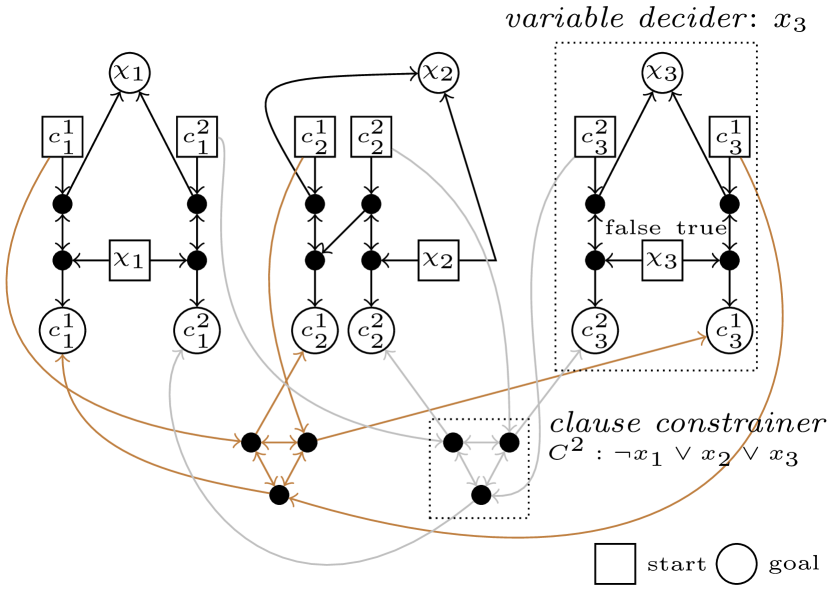
Figure 3: An OTIMAPP instance reduced from the 3-SAT formula $(x_{1}\lor x_{2}\lor\lnot x_{3})\land(\lnot x_{1}\lor x_{2}\lor x_{3})$.

Figure 4: A oneway constrainer. This gadget transforms an undirected edge $(u,v)$ to a directed one. Any agent is allowed to move only the way from $u$ to $v$ when limiting solutions to simple paths.

Theorem 4.2 (complexity on undirected graphs).

For OTIMAPP on undirected graphs, it is NP-hard to find a solution with simple paths.

Proof sketch.

We add a new gadget called oneway constrainer, which transforms an undirected edge to a virtually directed one, to the proof of the NP-hardness on digraphs (Thm. 4.1). We derive the claim by replacing all directed edges, except for bidirectional edges, with this gadget. Figure 4 illustrates it, including two new agents: $z_{1}$ and $z_{2}$. In this gadget, any agents outside of the gadget are allowed to move only in the direction from $u$ to $v$. ∎

4.2 Verification

The co-NP completeness of the verification relies on the following lemma, stating that finding cyclic deadlocks is computationally intractable. Its entire proof is delivered in the Appendix.

Lemma 4.3 (complexity of detecting cyclic deadlocks).

Determining whether a set of paths contains either reachable or potential cyclic deadlocks is NP-complete.

We then derive the complexity result since a solution has no reachable deadlocks.

Theorem 4.4 (complexity of verification).

Verifying a solutions of OTIMAPP is co-NP-complete.

Proof.

Thm. 3.5 states that a solution has no reachable terminal/cyclic deadlocks. Verifying no terminal deadlocks is in co-NP; a terminal deadlock is verified in polynomial time with an execution schedule. Verifying no potential deadlocks is co-NP-complete according to Lemma 4.3. ∎

5 Solvers

We now focus on how to solve OTIMAPP. In practice, it is difficult to use the necessary and sufficient condition (Thm. 3.5) because we have to find corresponding schedules. This motivates to build a relaxed sufficient condition.

Theorem 5.1 (relaxed condition).

Given an OTIMAPP instance, a set of path $\{\pi_{1},\ldots,\pi_{N}\}$ is a solution when there are (1) no use of other goals, i.e., $g_{j}\not\in\pi_{i}$ for all $i\neq j$ except for $s_{i}=g_{j}$, and (2) no potential cyclic deadlocks.

It is straightforward to see that the above conditions are respectively sufficient for the two conditions in Thm. 3.5. Given a set of paths, “no use of other goals” is easy to check while “no potential cyclic deadlocks” is intractable to compute (Lemma 4.3). Nevertheless, detecting potential cyclic deadlock is the heart of solving OTIMAPP. Thus, we first explain how to detect potential cyclic deadlocks. After that, two algorithms to solve OTIMAPP are presented.

5.1 Detection of Potential Deadlocks

Due to the space limit, we only describe the intuition behind the algorithm. The details are in the Appendix (Alg. 3). We first introduce a fragment, a candidate of potential cyclic deadlocks.

Definition 5.2 (fragment).

Given a set of paths $\{\pi_{1},$$\ldots,$$\pi_{N}\}$, a fragment is a tuple $\left((i,j,k,\ldots,l),(t_{i},t_{j},t_{k},\ldots,t_{l})\right)$ such that $\pi_{i}[t_{i}+1]=\pi_{j}[t_{j}]\land\pi_{j}[t_{j}+1]=\pi_{k}[t_{k}]\land\ldots=\pi_{l}[t_{l}]$. The elements of the first tuple are without duplicates.

We say that a fragment starts from a vertex $u$ when $\pi_{i}[t_{i}]=u$ and a fragment ends at a vertex $v$ when $\pi_{l}[t_{l}+1]=v$. A fragment that ends at its start (i.e., $\pi_{l}[t_{l}+1]=\pi_{i}[t_{i}]$) is a potential cyclic deadlock.

induction	key	new fragments
$\{\pi_{1}\}$	$u$	$\left[(1),(1),(u,v)\right]$
	$v$	$\left[(1),(2),(v,w)\right]$
$\{\pi_{1},\pi_{2}\}$	$u$	$\left[(1,2),(1,1),(u,v,x)\right]$
	$v$	$\left[(2),(1),(v,x)\right]$
	$x$	$\left[(2),(2),(x,y)\right]$
$\{\pi_{1},\pi_{2},\pi_{3}\}$	$u$	$\left[(1,2,3),(1,1,2),(u,v,x,u)\right]$
	$v$	$\left[(2,3),(1,2),(v,x,u)\right]$
	$x$	$\left[(3),(2),(x,u)\right]$, $\left[(3,1),(2,1),(x,u,v)\right]$
	$z$	$\left[(3),(1),(z,x)\right]$, $\left[(3,2),(1,2),(z,x,y)\right]$

Table 1: Example of detecting potential cyclic deadlocks. We describe the update of $\Theta_{\mathit{s}}$ for $\pi_{1}=(u,v,w),\pi_{2}=(v,x,y),\pi_{3}=(z,x,u)$. The table uses $[(\text{agents}),(\text{progress indexes}),(\text{path})]$ as a notation of fragment, where “path” is a corresponding sequence of vertices of the fragment. The algorithm halts with a blue-colored fragment, a detected potential cyclic deadlock.

Using fragments, we construct an algorithm to detect a potential cyclic deadlock in a set of paths if it exists. This is based on induction on $\pi_{i}$. The induction hypothesis for $i$ is that there are no potential cyclic deadlocks for $\{\pi_{1},\ldots,\pi_{i-1}\}$ and all fragments for them are identified. All new fragments about $\pi_{i}$ are categorized into three groups: (1) a fragment only with $\pi_{i}$, (2) a fragment that extends existing fragments, and (3) a fragment that connects existing two fragments. In either case, if a newly created fragment ends at its start, this is a deadlock.

The algorithm realizes this procedure by managing two tables that store fragments: $\Theta_{\mathit{s}}$ and $\Theta_{\mathit{t}}$. Both tables take one vertex as a key. One entry in $\Theta_{\mathit{s}}$ stores all fragments starting from the vertex. One entry in $\Theta_{\mathit{t}}$ stores all fragments ending at the vertex. Table 1 presents an example to detect deadlocks.

5.2 Prioritized Planning (PP)

Prioritized planning Erdmann and Lozano-Perez (1987); Silver (2005) is neither complete nor optimal, but it is computationally cheap hence a popular approach to MAPF. It plans paths sequentially while avoiding collisions with previously planned paths. Instead of inter-agent collisions, solvers for OTIMAPP have to care about potential cyclic deadlocks.

Algorithm 1 is prioritized planning for OTIMAPP, named PP. When planning a single-agent path, PP avoids using (1) goals of other agents and (2) edges causing potential cyclic deadlocks [Line 3]. The latter is detected by storing all fragments created by previously computed paths. For this purpose, PP uses the adaptive version of Alg. 3 [Line 5] in the Appendix. A path satisfying the constraints can be found by ordinary pathfinding algorithms. If not, PP returns FAILURE. The correctness of PP is derived from Thm. 5.1.

Algorithm 1 PP: Prioritized Planning

Input: an OTIMAPP instance
Output: a solution $\{\pi_{1},\ldots,\pi_{N}\}$ or FAILURE

1:$\Theta_{\mathit{s}},\Theta_{\mathit{t}}\leftarrow\emptyset$

2:for $i=1\ldots~{}|A|$ do

3:     $\pi_{i}\leftarrow\begin{aligned} &\text{a path for agent}~{}i~{}\text{while avoiding the use of}\\ &\cdot~{}g_{j},\forall j\neq i,\text{except for}~{}s_{i}\\ &\cdot~{}(u,v)\in E~{}\text{s.t.}~{}\exists\theta\in\Theta_{\mathit{t}}[u]~{}\text{and}~{}\theta~{}\text{starts from}~{}v\\ &\hskip 8.5359pt\triangleright\text{avoiding cyclic deadlocks for}~{}\pi_{j},j<i\end{aligned}$

4:     if $\pi_{i}$ is not found then return FAILURE

5:     update $\Theta_{\mathit{s}}$ and $\Theta_{\mathit{t}}$ with $\pi_{i}$ using Algorithm 3

6:end for

7:return $\{\pi_{1},\ldots,\pi_{N}\}$

PP is simple but incomplete. In particular, the planning order of agents is crucial; an instance may be solved or may not be solved as illustrated in Fig. 5. One resolution is repeating PP with random priorities until the problem is solved; let call this PP⁺. However, finding good orders can be challenging because there are $|A|!$ patterns. This motivates us to develop a search-based solver, described in the next.

Figure 5: Example that the planning order affects the solvability. When $i$ plans prior to $j$, PP results in success with solid lines. PP fails if $j$ plans first and takes the dotted line.

5.3 Deadlock-based Search (DBS)

We present deadlock-based search (DBS) to solve OTIMAPP, based on a popular search-based MAPF solver called conflict-based search (CBS) Sharon et al. (2015). CBS uses a two-level search. The high-level search manages collisions between agents. When a collision occurs between two agents at some time and location, two possible resolutions are depending on which agent gets to use the location at that time. Following this observation, CBS constructs a binary tree where each node includes constraints prohibiting to use space-time pairs for certain agents. In the low-level search, agents find a single path constrained by the corresponding high-level node.

Instead of collisions, DBS considers potential cyclic deadlocks. When detecting a deadlock in a set of paths, a resolution is that one of the agents in the deadlock avoids using the edge. Thus, the constraints identify which agents prohibit using which edges in which orientation.

Algorithm 2 DBS: Deadlock-based Search

Input: an OTIMAPP instance
Output: a solution $\{\pi_{1},\ldots,\pi_{N}\}$ or FAILURE

1:$R.\mathit{constraints}\leftarrow\emptyset$

2:$R.\mathit{paths}\leftarrow$ find paths with “no use of other goals”

3:insert $R$ to $\mathit{OPEN}$ $\triangleright$ $\mathit{OPEN}$: priority queue

4:while $\mathit{OPEN}\neq\emptyset$ do

5:     $N\leftarrow\mathit{OPEN}.\mathit{pop}()$

6:     $C\leftarrow$ get constraints of $N$ using Algorithm 3

7:     if $C=\emptyset$ then return $N.\mathit{paths}$

8:     for $(i,u,v)\in C$ do

9:         $N^{\prime}\leftarrow\begin{aligned} \{&\mathit{constraints}:N.\mathit{constraints}+(i,u,v),\\ &\mathit{paths}:N.\mathit{paths}\}\end{aligned}$

10:         update $\pi_{i}$ in $N^{\prime}.\mathit{paths}$ to follow $N^{\prime}.\mathit{constraints}$

11:         if $\pi_{i}$ is found then insert $N^{\prime}$ to $\mathit{OPEN}$

12:     end for

13:end while

14:return FAILURE

Algorithm 2 describes the high-level search of DBS. Each node in the high-level search contains constraints, a list of tuples consisting of one agent and two vertices (representing “from vertex” and “to vertex”), and paths as a solution candidate. The root node does not have any constraints [Line 1]. Its paths are computed following “no use of other goals” of Thm. 5.1 [Line 2]. Then, the node is inserted into a priority queue $\mathit{OPEN}$ [Line 3]. In the main loop [Line 4–13], DBS repeats; (1) Picking up one node [Line 5]. (2) Checking a deadlock and creating constraints [Line 6]. (3) Returning a solution if the paths contain no deadlocks [Line 7]. (4) If not, creating successors and inserting them to $\mathit{OPEN}$ [Line 8–12]. DBS returns FAILURE when $\mathit{OPEN}$ becomes empty [Line 14]. We complement several details below.

$\blacktriangleright$ Line 5: $\mathit{OPEN}$ is a priority queue and needs the order of nodes. DBS works in any order but good orders reduce the search effort. As effective heuristics, we use the descending order of the number of deadlocks with two agents, which is computed within a reasonable time.

$\blacktriangleright$ Line 6: Let $((i,j,k,\ldots,l),$$(t_{i},t_{j},t_{k},\ldots,t_{l}))$ be a returned deadlock by Alg. 3. Then, create constraints $(i,\pi_{i}[t_{i}],\pi_{i}[t_{i}+1]),(j,\pi_{j}[t_{j}],\pi_{j}[t_{j}+1]),\ldots,(l,\pi_{l}[t_{l}],\pi_{l}[t_{l}+1])$.

$\blacktriangleright$ Line 10: forces one path $\pi_{i}$ in the node to follow the new constraints. This low-level search must follow “no use of other goals,” furthermore, all edges in the constraints for $i$. If not found, DBS discards the corresponding successor.

Theorem 5.3 (DBS).

DBS returns a solution when solutions satisfying Thm. 5.1 exist; otherwise returns FAILURE.

Example

We describe an example of DBS using Fig. 5. Assume that the initial path of $i$ is the solid blue line and the path for $j$ is the dashed red line [Line 2]. This node is inserted into $\mathit{OPEN}$ [Line 3] and is expanded immediately [Line 5]. There is one potential cyclic deadlock in the paths then two constraints are created: either $i$ or $j$ avoids using the shared edge [Line 10]. Two child nodes are generated, however, the node that changes $i$’s path is invalid because there is no such path without the use of the goal of $j$. Another one is valid; $j$ takes the solid red line. Therefore, one node is added to $\mathit{OPEN}$ from the root node. In the next iteration, this newly added node is expanded. There are no potential cyclic deadlocks in this node; DBS returns its paths as a solution.

Optimization

Although this paper focuses on a feasibility problem, DBS can adapt to optimization problems. As objective functions, total path length and maximum path length in a solution can be defined. Those optimization problems are solved optimally by DBS when it prioritizes high-level search nodes with smaller scores, as commonly done in CBS. Note that metrics that assess time aspects such as total traveling time used in MAPF studies are significantly affected by execution schedules; the adaptation is not trivial.

6 Evaluation

This section empirically demonstrates that OTIMAPP solutions are computable to some extent (Sec. 6.1) and they are useful in adverse environments about timings (Sec. 6.2) through the simulation experiments. We also present OTIMAPP execution with robots (Sec. 6.3). The simulator was coded in C++ and the experiments were run on a desktop PC with Intel Core i9 $2.8\text{\,}\mathrm{GHz}$ CPU and $64\text{\,}\mathrm{GB}$ RAM.

6.1 Stress Test

Setup

Each solver was tested with a timeout of $5\text{\,}\mathrm{min}$ on four-connected undirected grids picked up from Stern et al. (2019), as a graph $G$. We also tested random graphs, shown in the Appendix. All instances were generated by setting a start $s_{i}$ and a goal $g_{i}$ randomly while ensuring that $s_{i}$ and $g_{i}$ have at least one path without the use of other goals; otherwise, it violates “no use of other goals” of Thm. 5.1. Note that unsolvable instances might still be included.

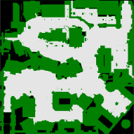
random-32-32-10 $32{\times}32~{}(922)$	random-64-64-10 $64{\times}64~{}(3687)$	den520d $256{\times}257~{}(28178)$

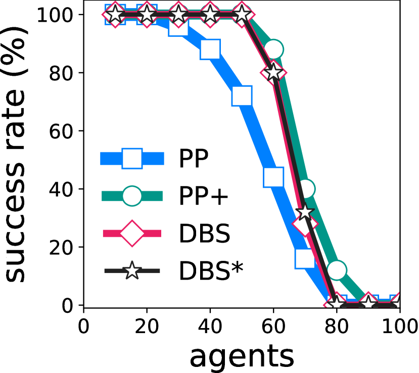
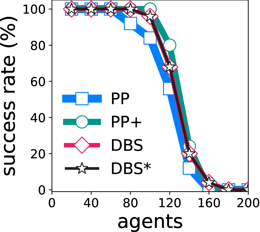
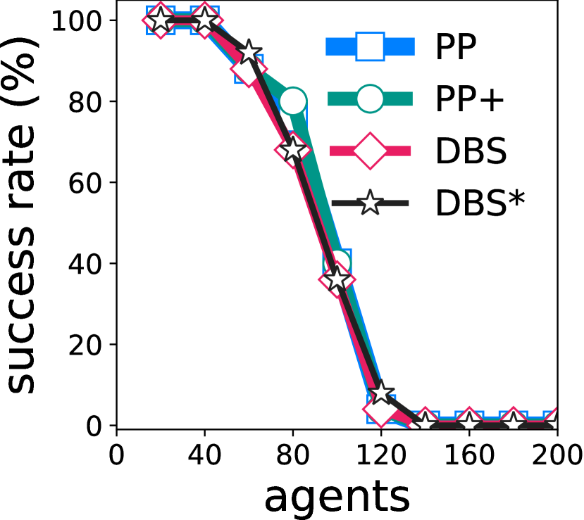
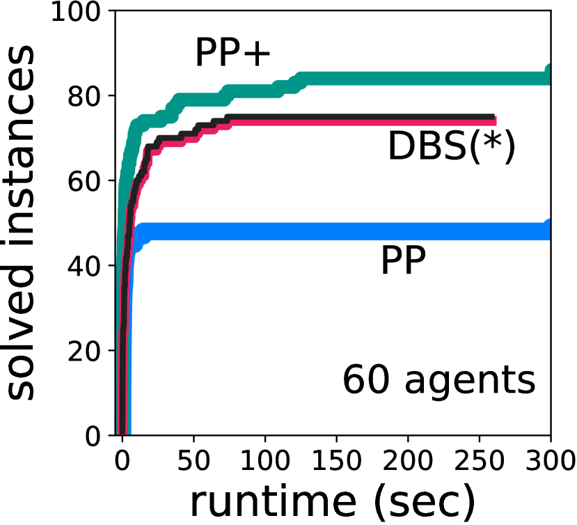
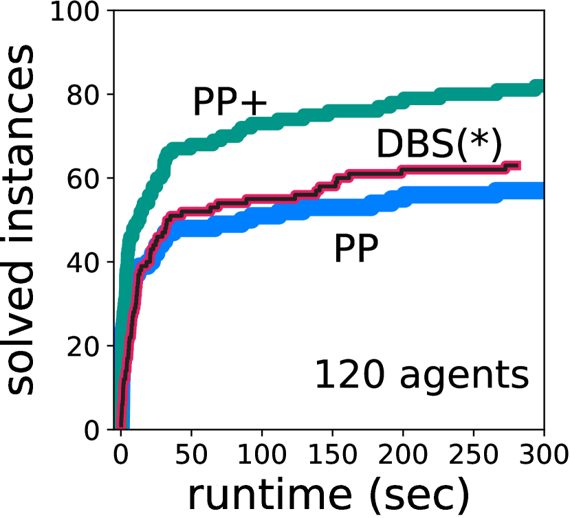
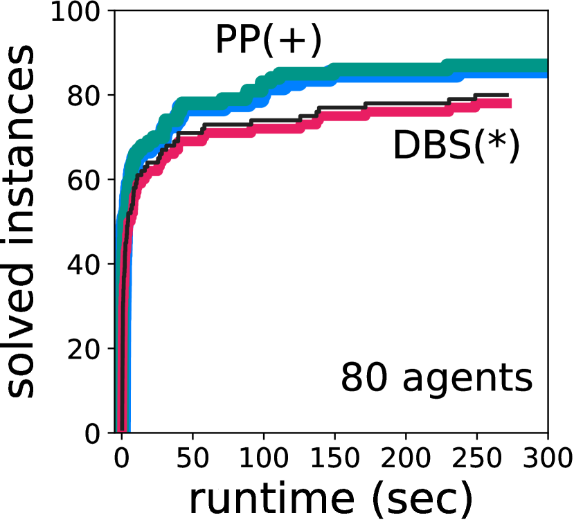
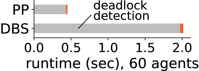
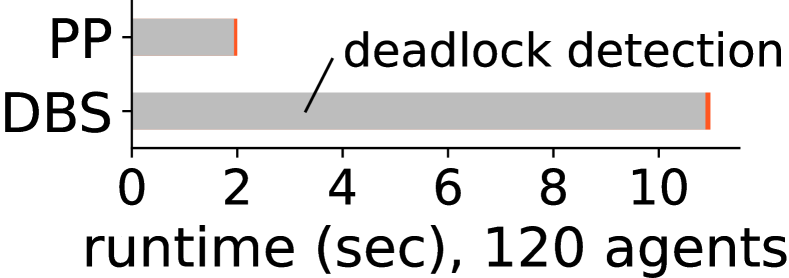
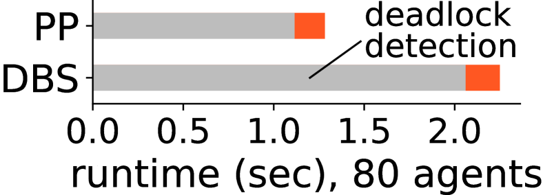
Figure 6: Stress test on 4-connected grids. The success rate is based on 25 identical instances. DBS^∗ includes detected instances that are unsolvable for DBS before timeout, which is not possible for PP⁽⁺⁾. We also present accumulated runtime with a fixed number of agents over 100 instances, and runtime profiling (median) of each solver over success instances for both solvers.

Result

Fig. 6 presents the results. The main findings are: (1) Both solvers can solve instances with tens of agents in various maps within a reasonable time. (2) PP often fails due to priority orders (e.g., Fig. 5) while PP⁺ and DBS can overcome such limitations to some extent. (3) A bottleneck of each solver is the procedure of detecting potential cyclic deadlocks, an NP-hard problem (Lemma. 4.3). This also leads to similar success rates of PP⁺ and DBS.

6.2 Delay Tolerance

We next show that OTIMAPP solutions (if found) are useful in a simulated environment with stochastic delays of agents’ moves built on conventional MAPF, called MAPF-DP (with Delay Probabilities) Ma et al. (2017). Given a graph and start-goal pairs for each agent, the aim of MAPF is to move agents to their goals without collisions. Collisions occur when two agents occupy the same vertex or traverse the same edge simultaneously. Time is discrete. All agents synchronously take actions, i.e., either move to an adjacent vertex or stay at the current location. MAPF-DP emulates the imperfect execution of MAPF by introducing the possibility $p_{i}$ of unsuccessful moves for agent $i$ (remaining there).

Setup

The delay probabilities $p_{i}$ were chosen uniformly at random from $[0,\bar{p}]$, where $\bar{p}$ is the upper bound of $p_{i}$. The higher $\bar{p}$ means that agents delay often, and vice versa. The metric is the total traveling time of agents; smaller values mean less wasting time at runtime. We tested the following two as baselines: (1) MCPs Ma et al. (2017) force agents to preserve order relations of visiting one vertex in an offline MAPF plan at runtime. The plan was obtained by ECBS Barer et al. (2014). (2) Causal-PIBT Okumura et al. (2021) is online time-independent planning, that is, each agent repeats one-step planning and action adaptively to surrounding current situations. The other details are in the Appendix.

Result

Table 2 shows that the execution of OTIMAPP solutions outperforms the alternatives. This is because: (1) Unlike MCPs, OTIMAPP solutions are free from temporal dependencies of offline plans that one agent delays are possibly fatal. (2) Unlike Causal-PIBT, agents follow long-term plans and avoid possible congested locations.

Discussion

Although finding OTIMAPP solutions is challenging, Table 2 motivates us to compute them. Meanwhile, the other approaches can solve larger instances with more agents (e.g., $|A|=200$) and with much smaller planning time than solving OTIMAPP. Moreover, there are situations where OTIMAPP has no solutions while the others can find feasible plans because OTIMAPP assumes no intervention at runtime. One future direction pursues to fill these gaps.

$|A|=35$	$\bar{p}=0.2$		$\bar{p}=0.5$		$\bar{p}=0.8$
MCPs+ECBS	1015	(1004,1026)	1422	(1404,1440)	2551	(2507,2596)
Causal-PIBT	986	(976,995)	1238	(1225,1250)	1841	(1816,1866)
OTIMAPP	941	(931,951)	1178	(1165,1190)	1730	(1707,1752)
$\bar{p}=0.5$	$|A|=20$		$|A|=40$		$|A|=60$
MCPs+ECBS	724	(711,736)	1698	(1678,1716)	2938	(2911,2964)
Causal-PIBT	662	(653,671)	1466	(1453,1479)	2425	(2405,2444)
OTIMAPP	639	(631,648)	1395	(1383,1408)	2328	(2311,2345)

Table 2: Total traveling time on MAPF-DP. All settings used random-32-32-10. For each setting, we first picked up 10 instances that OTIMAPP solutions were found by PP⁺. For each instance and approach, we then performed 50 trials while changing the random seed. Thus, the scores are means on 500 executions, accompanied with 95% confidence intervals. upper: Results of changing $\bar{p}$ while fixing $|A|$. lower: Results of changing $|A|$ while fixing $\bar{p}$. Note that the probability that someone delays increases with more agents.

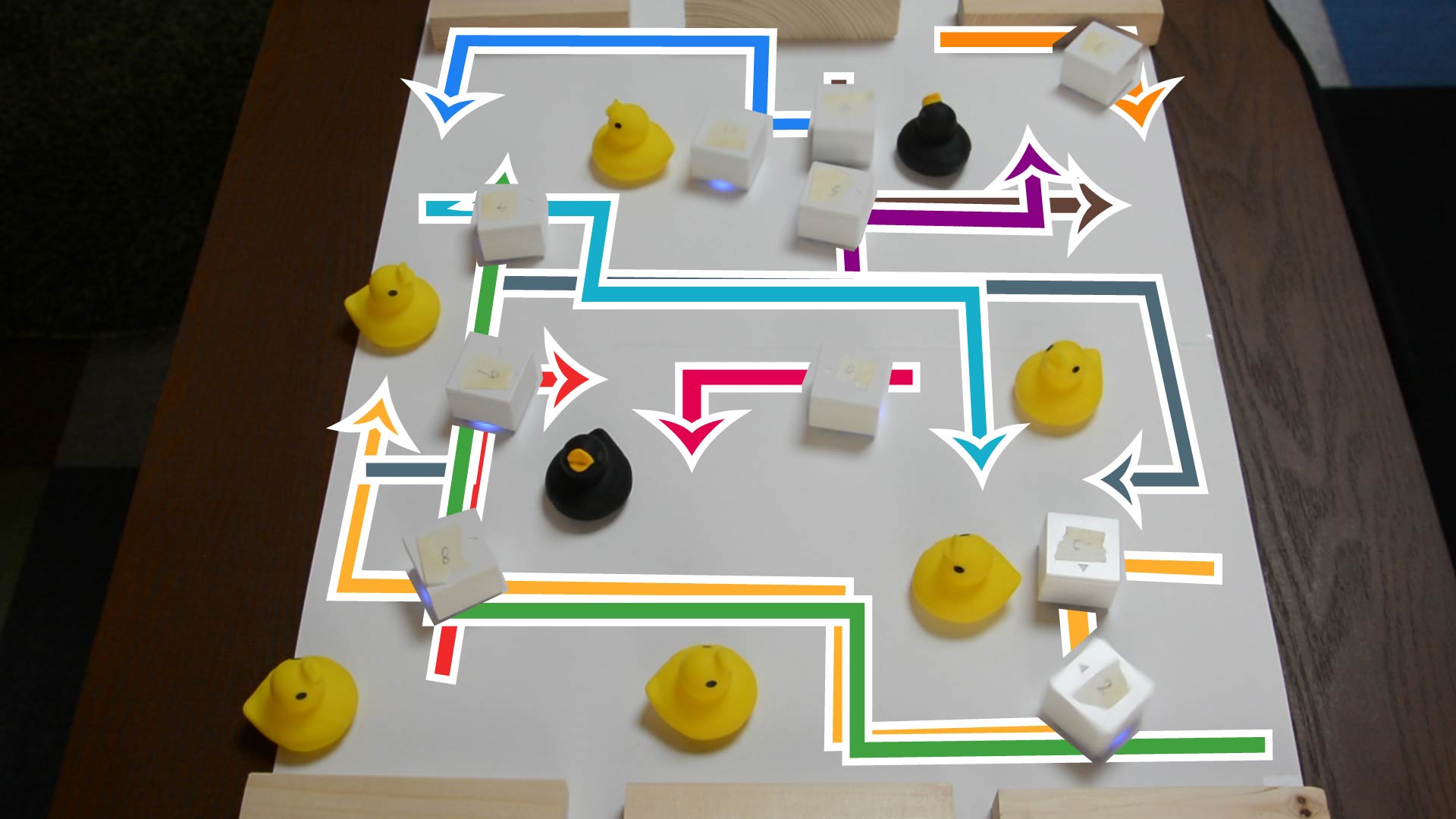
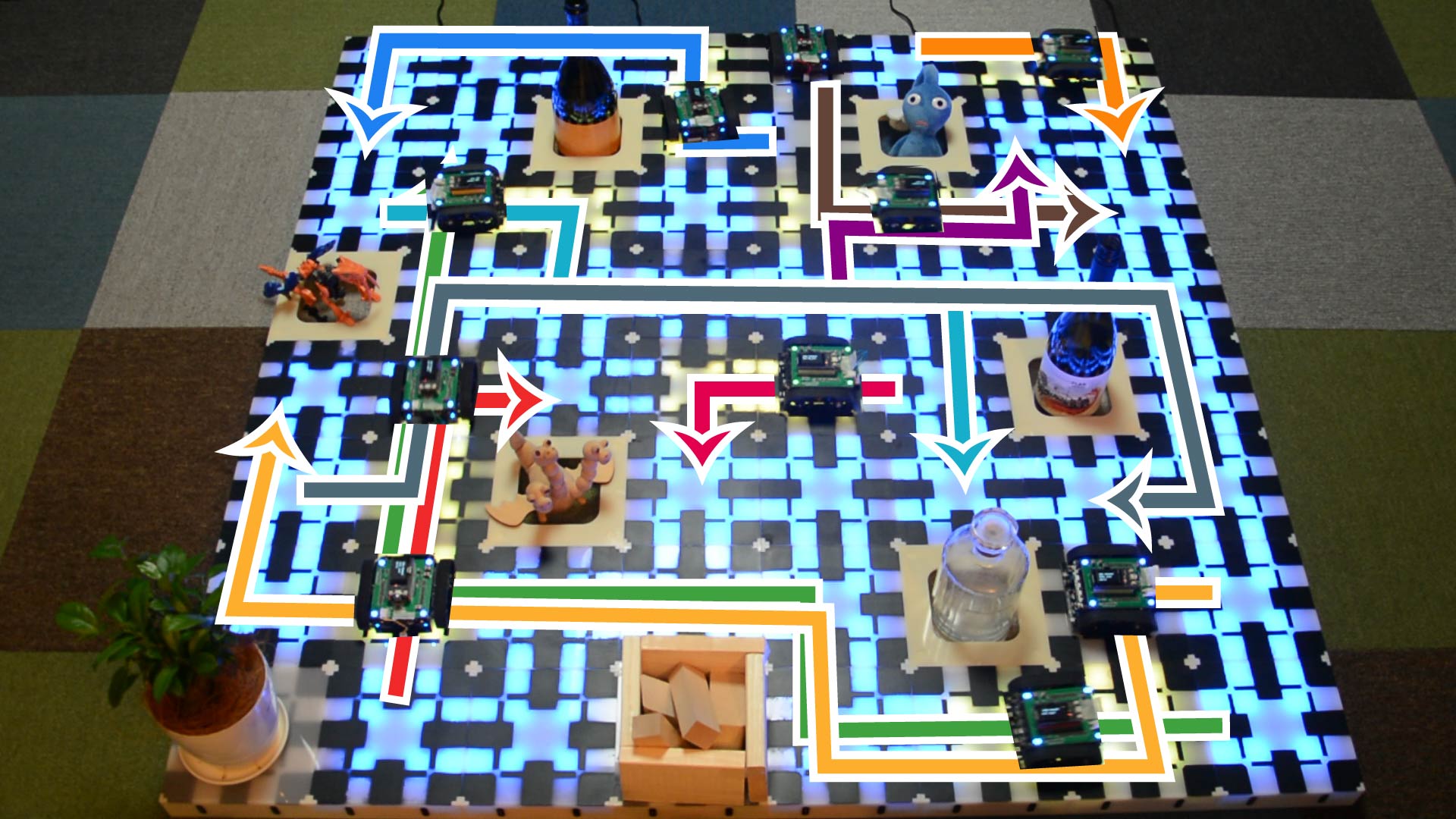
Figure 7: An OTIMAPP execution with $10$ robots in an $8\times 8$ grid. Colored arrows represent an OTIMAPP solution.

6.3 Robot Demonstrations

We present two OTIMAPP execution styles: (1) a centralized control using the toio robots (https://toio.io) and (2) a decentralized one with only local interactions using a multi-robot platform Kameyama et al. (2021). A solution was obtained by DBS. Figure 7 is snapshots. A video is available online. In both cases, robots move without any synchronization procedures but are ensured to eventually reach their goals thanks to the nature of OTIMAPP. Moreover, for the latter, any actor has no methods to know the entire configuration, which cannot be addressed by conventional execution strategies.

7 Related Work

A deadlock Coffman et al. (1971) is a widely recognized phenomenon not limited to robotics; a system state that several components claim resources that others hold, then block each other permanently. Strategies to cope with deadlocks are categorized into prevention, detection/recovery, and avoidance Silberschatz et al. (2006); Fanti and Zhou (2004); OTIMAPP is prevention. A non-deadlock state that is “inevitable” to reach deadlocks is called unsafe Silberschatz et al. (2006). Meanwhile, reachable deadlocks of OTIMAPP correspond to states that are “possible” to reach deadlocks. The notion of potential terminal deadlock is related to well-formed instances of MAPF Čáp et al. (2015), that is, for each start-goal pair, a path exists that traverses no other starts and goals. The notion of reachable cyclic deadlock is mentioned as nonlive states/sets for deadlock management in automated manufacturing systems Fanti and Zhou (2004) or in a multi-robot scheduling problem Mannucci et al. (2021).

The multi-agent pathfinding (MAPF) problem Stern et al. (2019) aims at finding a set of collision-free paths on a graph. Many studies on MAPF consider timing uncertainties because they are inevitable in multi-agent scenarios. However, current methods largely rely on additional assumptions on the travel speed of agents or assume delays to follow some probability distributions Wagner and Choset (2017); Mansouri et al. (2019); Peltzer et al. (2020); Atzmon et al. (2020a). Failing to represent the inherent uncertainty in the domain means the system behavior can be unpredictable. Alternative approaches are online intervention during execution, e.g., forcing agents to preserve temporal dependencies of offline planning via communication Ma et al. (2017); Hönig et al. (2019); Atzmon et al. (2020b). Another direction is online time-independent planning Okumura et al. (2021) that incrementally moves agents based on current situations. OTIMAPP shares the concept of time independence but aims at offline planning without or less runtime effort.

In graph theory, the (vertex) disjoint path problem and its variants Robertson and Seymour (1985) are partly related to ours in the sense that a set of disjoint paths clearly satisfies the solution condition of OTIMAPP, but the reverse does not.

8 Conclusion

This paper studied a novel path planning problem called OTIMAPP, motivated by the nature of distributed environments (i.e., timing uncertainties) that multi-agent systems must address. We focused on robotic applications in evaluation but believe that OTIMAPP can be leveraged to other resource allocation problems with mutual exclusion, e.g, distributed databases, which is our future direction.

Appendix

We complement omitted proofs (Sec. A, B, and D), the detailed procedure of detecting potential cyclic deadlocks (Sec. C), additional results of stress test on random graphs (Sec. E), and the details of experimental setups (Sec. F).

Appendix A Proof of Solution Analysis

Theorem (3.5; necessary and sufficient condition).

Given an OTIMAPP instance, a set of path $\{\pi_{1},\ldots,\pi_{N}\}$ is a feasible solution if and only if there are:

• No reachable terminal deadlocks.

• No reachable cyclic deadlocks.

Proof.

Without “no reachable terminal deadlocks,” there is an execution that one agent arrives at its goal and remains there; disturbing the progression of another agent. Without “no reachable cyclic deadlocks,” a cyclic deadlock might occur and those agents stop the progression. Hence those two are necessary.

We now prove that the two conditions are sufficient. Given a solution candidate $\{\pi_{1},\ldots,\pi_{N}\}$ with no reachable deadlocks, consider the potential function $\phi\mathrel{\mathop{:}}=\sum_{i\in A}(|\pi_{i}|-\mathit{clock}_{i})$ defined over a configuration $\{\mathit{clock}_{1},\ldots,\mathit{clock}_{N}\}$. Observe that $\phi$ is non-increasing and $\phi=0$ means that all agents have reached their goals. Furthermore, when $\phi>0$, $\phi$ is guaranteed to decrease if each agent is activated at least once. We explain this as follows.

Suppose contrary that $\phi(\neq 0)$ does not differ for the period. Since $\phi\neq 0$, there are agents whose progress indexes are less than the maximum values. Let them $B\subseteq A$. For an agent $i\in B$, $\pi_{i}[\mathit{clock}_{i}+1]$ is occupied by another agent $j\in B$, according to “no reachable terminal deadlocks,” otherwise, $i$ moves there. This is the same for $j$, i.e., there is an agent $k\in B$ such that $\pi_{j}[\mathit{clock}_{j}+1]=\pi_{k}[\mathit{clock}_{k}]$. By induction, this sequence of agents must form a cycle somewhere, i.e., occurring a cyclic deadlock; however, this contradicts “no reachable cyclic deadlocks.”

Each agent is activated at least once in a sufficiently long period due to the fair assumption, deriving the statement. ∎

Appendix B Proofs of Computational Complexity

Theorem (4.2; complexity on undirected graphs).

For OTIMAPP on undirected graphs, it is NP-hard to find a feasible solution with simple paths.

Proof.

We add a new gadget, which makes an undirected edge to a virtually directed one, to the proof of the NP-hardness on digraphs (Thm. 4.1). We derive the claim by replacing all directed edges, except for bidirectional edges, with this gadget.

Figure 3 (right) is it, including two new agents: $z_{1}$ and $z_{2}$. In this gadget, any agents outside of the gadget are allowed to move only the direction from $u$ to $v$. Assume contrary that, one agent ($\neq z_{1},z_{2}$) takes a path through $v$ to $u$ within this gadget, and there is another path from $v$ to $u$. To avoid cyclic deadlocks, $z_{1}$ and $z_{2}$ must move toward the left side, exit the gadget from $u$, use another path to enter $v$, and eventually reach their goals. In these paths, $z_{1}$ can arrive at its goal earlier than that of $z_{2}$, contradicting “no reachable terminal deadlocks” in the necessary and sufficient condition (Thm. 3.5). Therefore, these paths are invalid.

The size of the OTIMAPP instance is still polynomial on the 3-SAT formula. Thus, we conclude the statement.

Note that, if we allow non-simple paths, it might be possible for other agents to move through the way from $v$ to $u$. This is because, even though $z_{1}$ and $z_{2}$ temporarily leave from the gadget via $u$, we can construct paths that $z_{1}$ always arrive at its goal after $z_{2}$’s arrival, as illustrated in Fig. 8. ∎

Figure 8: Counterexample of oneway constrainer without assmptions of simple paths. $z_{2}$ always arrives at its goal before the arrival of $z_{1}$ if those two agents follow colored lines.

Figure 9: OTIMAPP instance and solution reduced from the 3-SAT instance $(x_{1}\lor x_{2}\lor\lnot x_{3})\land(\lnot x_{1}\lor x_{2}\lor x_{3})\land(x_{1}\lor\lnot x_{2}\land\lnot x3)$. For visualization, we break a large circle; regard two $\clubsuit$ marks as connected. Omitted vertices and edges are complemented in Fig. 10.

Figure 10: Complete version of Fig. 9 for $(x_{1}\lor x_{2}\lor\lnot x_{3})\land(\lnot x_{1}\lor x_{2}\lor x_{3})\land(x_{1}\lor\lnot x_{2}\land\lnot x3)$. Each color corresponds to a path for each agent.

Lemma (4.3; complexity of detecting cyclic deadlocks).

Determining whether a set of paths contains either reachable or potential cyclic deadlocks is NP-complete.

Proof.

The proof is a reduction from the 3-SAT problem, i.e., constructing a combination of an OTIMAPP instance and a set of paths such that potential cyclic deadlocks exist if and only if the corresponding formula is satisfiable. We show the case of directed graphs. The proof procedure applies to the undirected case without modifications. In addition, all potential cyclic deadlocks are reachable in the translated problem. The reduction is done in polynomial time, deriving the NP-hardness of detecting both reachable and potential cyclic deadlocks. Since a potential cyclic deadlock can be verified in polynomial time, and since a reachable cyclic deadlock can be verified in polynomial time with an execution schedule, they are NP-complete.

We now explain how to translate the 3-SAT formula to the OTIMAPP instance and the corresponding set of paths. Without loss of generality, we assume that all variables appear positively and negatively in the formula. Throughout the proof, we use the following example.

$$(x_{1}\lor x_{2}\lor\lnot x_{3})\land(\lnot x_{1}\lor x_{2}\lor x_{3})\land(x_{1}\lor\lnot x_{2}\land\lnot x_{3})$$

Its outcome is partially depicted in Fig. 9. The complete version is presented in Fig. 10.

A. Construction of an OTIMAPP instance and a set of paths For each literal in each clause, one literal agent is introduced. We denote by $c^{j}_{k}$ a literal agent for the $k$-th literal in $j$-th clause $C^{j}$ in the formula. We also use one special agent $z$.

Next, consider two gadgets: variable decider and clause constrainer. Note that they are different from those used in the proof of Thm. 4.1; however, their intuitions are similar and we use the same names.

The variable decider determines whether a variable $x_{i}$ occurs positively or negatively. For each variable one gadget is introduced. All literal agents for $x_{i}$ (i.e., either $x_{i}$ or $\lnot x_{i}$) start from vertices in this gadget. The gadget contains two paths: an upper path, corresponding to assign true to $x_{i}$, and a lower path, corresponding to assign false to $x_{i}$. Positive literals are connected to the upper path. Negative literals are connected to the lower path. For instance, $x_{2}$ has three literal agents: $c^{1}_{2}$ ($x_{2}$), $c^{2}_{2}$ ($x_{2}$), and $c^{3}_{2}$ ($\lnot~{}x_{2}$). In Fig. 9, we highlight the upper and the lower paths by bold lines. $c^{1}_{2}$ and $c^{2}_{2}$ are connected to the upper path while $c^{3}_{2}$ is connected to the lower path. Each literal agent uses one edge in the upper/lower path and moves to a clause constrainer via one vacation vertex.

The clause constrainer contains all goals of the literal agents in the clause. Three edges are used to reach the goals. Each edge is for each literal agent. For instance, the clause constrainer of $C^{2}$ contains the goals of $c^{2}_{1}$, $c^{2}_{2}$, and $c^{2}_{3}$. In Fig. 9, three edges are annotated with the agent’s name. $c_{2}^{2}$ is supposed to use the colored middle one. Note that we use multiple edges for simplicity. It is not hard to convert the gadget to a simple graph version, as shown immediately later of this proof.

As a result, all literal agents take six edges to reach their goals. This is visualized by colored edges in Fig. 9 and Fig. 10. The special agent $z$ uses two edges to reach its goal, through $\clubsuit$ marks in the figure. We finish the description of how to construct the OTIMAPP instance and the corresponding set of paths. The remaining part is to show these paths contain potential/reachable cyclic deadlocks if and only if the formula is satisfiable. This translation from the formula is clearly done in polynomial time.

B. A potential cyclic deadlock exists if the formula is satisfiable. To see this, observe that if a potential cyclic deadlock exists, agents must try to use; (a) either an upper or a lower path for each variable decider, (b) one edge for each clause constrainer, and (c) the edge for $z$ ($\clubsuit$).

Step 1: Move assigned agents to vacation vertices

Step 2: Fill clause constrainers

Step 3: Move unassigned agents one step

Figure 11: Construction of a reachable deadlock. The formula is $(x_{1}\lor x_{2}\lor\lnot x_{3})\land(\lnot x_{1}\lor x_{2}\lor x_{3})\land(x_{1}\lor\lnot x_{2}\land\lnot x3)$. The assignment is $x_{1}=\mathit{true}$, $x_{2}=\mathit{true}$, and $x_{3}=\mathit{true}$. Locations of all agents are colored. When an agent departs from its start, the corresponding vertex is filled by dark. Bold lines in Step 3 constitute a reachable deadlock.

When the formula is satisfiable for one assignment, consider the following execution.

1. For each assigned value, move the corresponding clause agents to vacation vertices in each variable decider, i.e., one step before clause constrainers.

2. Among the above agents, for each clause constrainer, there is at least one agent that can enter the clause constrainer due to satisfiability. Move them one step further. As a result, all clause constrainers have one agent at the first vertices. Vertices in upper/lower paths in the variable deciders must be vacant now.

3. Move all unassigned clause agents one step. As a result, all vertices in the unassigned paths are filled by the unassigned clause agents.

We now have a cyclic deadlock, i.e., this deadlock is reachable thus potential.

As an example, consider a satisfiable assignment $x_{1}=\mathit{true}$, $x_{2}=\mathit{true}$, $x_{3}=\mathit{true}$. In the beginning, move assigned agents, $c^{1}_{1}$, $c^{1}_{2}$, $c^{2}_{2}$, $c^{2}_{3}$, and $c^{3}_{1}$ to vacation vertices in each variable decider (Fig. 11; Step 1). Next, move $c^{1}_{2}$, $c^{2}_{2}$, and $c^{3}_{1}$ to the first vertices of each clause constrainer of $C^{1}$, $C^{2}$, and $C^{3}$, respectively (Fig. 11; Step 2). Then, move all unassigned agents, $c^{2}_{1}$, $c^{3}_{2}$, $c^{1}_{3}$, and $c^{3}_{3}$, one step (Fig. 11; Step 3). There is a cyclic deadlock with $c^{2}_{1},c^{3}_{2},c^{1}_{3},c^{3}_{3},c^{1}_{2},c^{2}_{2},c^{3}_{1}$, and $z$, annotated with bold lines in Fig. 11.

C. The formula is satisfiable if a potential cyclic deadlock exists. To form a potential cyclic deadlock, for each variable decider, one or several agents try to move along either an upper or a lower path. Consider assigning an opposite value against the used path to the variable. For instance, if $c^{1}_{2}$ and $c^{2}_{2}$ involve in the deadlock at the variable decider (see Fig. 9), then assign $\mathit{false}$ to $x_{2}$. This assignment must satisfy the formula because at least one literal in each clause becomes true; otherwise, at least one clause constrainer exists such that the first vertex is empty, i.e., no deadlock.

D. All potential cyclic deadlocks are reachable. So far, we established the claim that a potential cyclic deadlock exists if and only if the formula is satisfiable. Next, we claim that all potential cyclic deadlocks are reachable. According to the above discussion, given a potential cyclic deadlock, the corresponding satisfiable assignment exists. Consider the execution of Part B using this assignment, slightly changing Step 2. In this step, we can choose arbitrary agents for each clause constrainer. Therefore, it is possible to choose agents involved in the potential cyclic deadlock. As a result, this deadlock is reachable. ∎

Figure 12: Example of clause constrainer without multiple edges. Used in the proof of Lemma 4.3.

In the proof of Lemma 4.3, we used multiple edges in a gadget clause constrainer for the reduction from 3-SAT. Since OTIMAPP assumes a simple graph (i.e., no multiple edges), we complement how to convert it to a correct OTIMAPP instance. Figure 12 shows an example of the clause constrainer for $C^{2}$. Recall that a clause constrainer contains all goals for the corresponding clause agents. In this new gadget, we add intermediate vertices for each edge that potentially leads to cyclic deadlocks. For each agent $c^{j}_{k}$, a new agent $\hat{c}^{j}_{k}$ is introduced. Its start is the intermediate vertex. Its goal is the original goal of $c^{j}_{k}$. We furthermore change a goal for $c^{j}_{k}$ to starts of $\hat{c}^{j}_{k}$. Consider now replacing all old clause constrainers with this new gadgets. The translation is done in polynomial time. The rest of the proof is straightforward from Lemma 4.3.

Appendix C Detecting Potential Cyclic Deadlocks

Algorithm 3 Potential Cyclic Deadlock Detection

Input: a set of paths $\{\pi_{1},\ldots,\pi_{n}\}$
Output: one potential cyclic deadlock or NONE

1:$\Theta_{\mathit{s}},\Theta_{\mathit{t}}\leftarrow\emptyset$ $\triangleright$ table for fragments, key: vertex

2:procedure register($\theta$)

3:    $i,t_{i},j,t_{j}\leftarrow\theta.\{\text{agents},\text{indexes}\}\{[1],[-1]\}$

4:    $\Theta_{\mathit{s}}[\pi_{i}[t_{i}]]$.append($\theta$)

5:    $\Theta_{\mathit{t}}[\pi_{j}[t_{j}+1]]$.append($\theta$)

6:end procedure

7:function isPotentialDeadlock($\theta$)

8:    $i,t_{i},j,t_{j}\leftarrow\theta.\{\text{agents},\text{indexes}\}\{[1],[-1]\}$

9:    return $\pi_{i}[t_{i}]=\pi_{j}[t_{j}+1]$

10:end function

11:for $i=1\ldots n$ do

12:    for $j=1\ldots|\pi_{i}|-1$ do

13:         $u\leftarrow\pi_{i}[j],v\leftarrow\pi_{i}[j+1]$

14:         $\theta\leftarrow\left\{\text{agents:}~{}(i),~{}\text{indexes:}~{}(j)\right\}$ $\triangleright$ single fragment

15:         register($\theta$)

16:         for $\theta_{\mathit{t}}\in\Theta_{\mathit{t}}[u]$ do $\triangleright$ check fragments on $\Theta_{\mathit{t}}$

17:             if $i\in\theta_{\mathit{t}}.\text{agents}$ then continue

18:             $\theta\leftarrow\left\{\text{agents:}~{}\theta_{\mathit{t}}.\text{agents}+i,~{}\text{indexes:}~{}\theta_{\mathit{t}}.\text{indexes}+j\right\}$

19:             if isPotentialDeadlock($\theta$) then return $\theta$

20:             register($\theta$)

21:         end for

22:         for $\theta_{\mathit{f}}\in\Theta_{\mathit{s}}[v]$ do $\triangleright$ check fragments on $\Theta_{\mathit{s}}$

23:             if $i\in\theta_{\mathit{f}}.\text{agents}$ then continue

24:             $\theta\leftarrow\begin{aligned} \{\text{agents:}~{}i+\theta_{\mathit{f}}.\text{agents},\text{indexes:}~{}j+\theta_{\mathit{f}}.\text{indexes}\}\end{aligned}$

25:             if isPotentialDeadlock($\theta$) then return $\theta$

26:             register($\theta$)

27:         end for

28:         for $\theta_{\mathit{t}}\in\Theta_{\mathit{t}}[u]$, $\theta_{\mathit{f}}\in\Theta_{\mathit{s}}[v]$ do $\triangleright$ connect two fragments

29:             if $i\in\theta_{\mathit{t}}.\text{agents}\cup\theta_{\mathit{f}}.\text{agents}$ then continue

30:             if $\theta_{\mathit{t}}.\text{agents}\cap\theta_{\mathit{f}}.\text{agents}\neq\emptyset$ then continue

31:             $\theta\leftarrow\begin{aligned} \{&\text{agents:}~{}\theta_{\mathit{t}}.\text{agents}+i+\theta_{\mathit{f}}.\text{agents}\\ &\text{indexes:}~{}\theta_{\mathit{t}}.\text{indexes}+j+\theta_{\mathit{f}}.\text{indexes}\}\end{aligned}$

32:             if isPotentialDeadlock($\theta$) then return $\theta$

33:             register($\theta$)

34:         end for

35:    end for

36:end for

37:return NONE

Using fragments, Alg. 3 detects a potential cyclic deadlock in a set of paths if exists. The intuition is the following: (1) the algorithm checks each path one by one, (2) it stores all fragments created so far, (3) for each edge in each path, it creates new fragments using existing fragments, and (4) if a fragment ends at its start, this is a potential cyclic deadlock. We describe the details in the proof of the completeness.

Theorem C.1 (completeness).

Alg. 3 finds one potential cyclic deadlock if exists, otherwise returns NONE.

Proof.

The algorithm uses two tables that store fragments: $\Theta_{\mathit{s}}$ and $\Theta_{\mathit{t}}$. Both tables take one vertex as a key. One entry in $\Theta_{\mathit{s}}$ stores all fragments starting from the vertex. One entry in $\Theta_{\mathit{t}}$ stores all fragments ending at the vertex. A fragment is registered in both tables. We now derive the statement by induction on $\pi_{i}$.

Base case: At the first iteration of the loop [Line 11–36], all fragments for $\{\pi_{1}\}$ are registered on $\Theta_{\mathit{s}}$ and $\Theta_{\mathit{t}}$ due to Line 14–15. There are no potential cyclic deadlocks for $\{\pi_{1}\}$.

Induction Hypothesis: Assume that there are no potential cyclic deadlocks for $\{\pi_{1},\ldots,\pi_{i-1}\}$ and all fragments for them are registered on $\Theta_{\mathit{s}}$ and $\Theta_{\mathit{t}}$.

Induction Step: We now show the property for $i$; otherwise, a potential cyclic deadlock exists for $\{\pi_{1},\ldots,\pi_{i}\}$ and the algorithm returns it. All new fragments about $\pi_{i}$ are categorized into two: (1) a fragment only with $\pi_{i}$ or (2) a fragment that extends other fragments on $\Theta_{\mathit{s}}$ and $\Theta_{\mathit{t}}$, using $(u,v)\in\pi_{i}$. The former is preserved due to Line 14–15. The latter is further categorized into three cases: (a) a fragment ends at $v$, (b) a fragment starts from $u$, and (c) a fragment connecting two existing fragments that one ends at $u$ and another starts from $v$. Each case corresponds to Line 16–21, Line 22–27, and Line 28–34, respectively. As a result, all fragments are to register on $\Theta_{\mathit{s}}$ and $\Theta_{\mathit{t}}$; otherwise, a potential cyclic deadlock exists and the algorithm returns it [Line 19, 25, and 32]. ∎

The time complexity does not contradict the NP-completeness of detecting potential deadlocks (Lemma 4.3).

Proposition C.2 (space and time complexity).

Algorithm 3 requires $\Omega(2^{|n|})$ both for space and time complexity in the worst case.

Proof.

Consider an example in Fig. 13. In any solutions, the number of fragments starting from $u$ becomes $\Omega\left(2^{|n|}\right)$; this implies the statement. ∎

Although Alg. 3 does not run in polynomial time, it works sufficiently fast in a sparse environment such that not many paths use the same vertices.

Figure 13: Example that requires huge space and time to detect potential deadlocks. All starts are on the left. All goals are on the right. Two zones are connected by a sufficiently long path.

Appendix D Proof of DBS

Theorem (5.3; DBS).

DBS returns a solution when solutions satisfying Thm. 5.1 exist; otherwise returns FAILURE.

Proof.

Assume that there is a solution $\mathbf{\pi}=\{\pi_{1},\ldots,\pi_{N}\}$ satisfying the relaxed sufficient condition (Thm. 5.1). At each cycle [Line 4–13], at least one node in $\mathit{OPEN}$ is consistent with $\mathbf{\pi}$, i.e., its constraints allow searching $\mathbf{\pi}$. This is derived by induction: (1) the initial node $R$ is consistent with $\mathbf{\pi}$, and (2) generated nodes from a consistent node with $\mathbf{\pi}$ must include at least one consistent node. The search space, i.e., which agents are prohibited using which edges in which directions, is finite. Therefore, DBS eventually returns $\mathbf{\pi}$ (or another solution); otherwise, such solutions do not exist. ∎

Appendix E Stress Test on Random Graphs

$G(1000,0.003)$	$G(1000,0.004)$	$G(1000,0.005)$

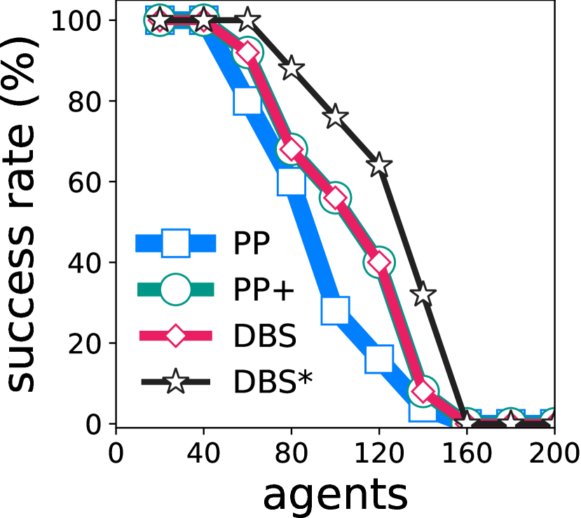
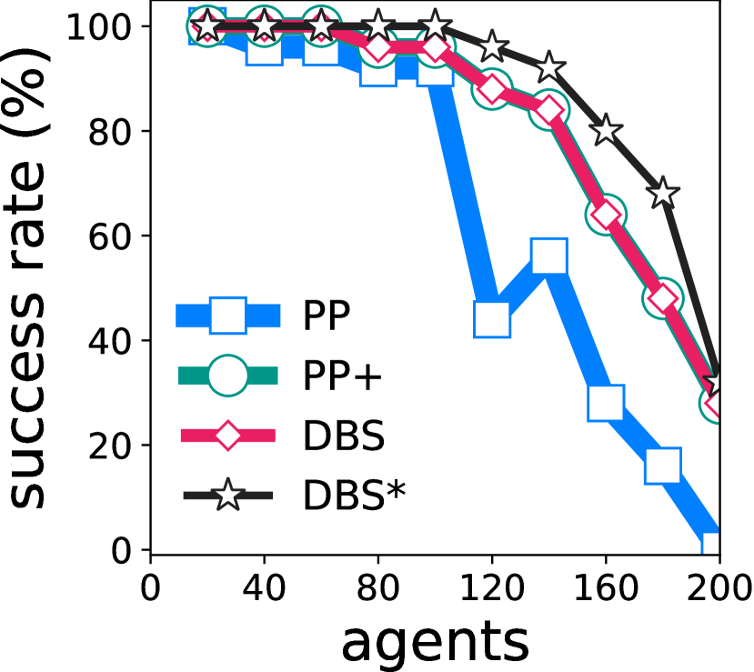
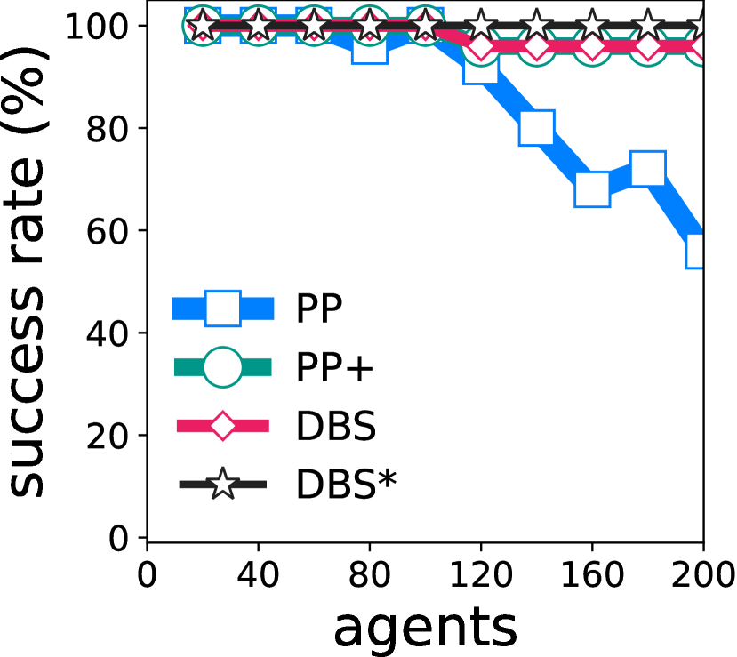
Figure 14: Stress test of random graphs. The success rate is based on 25 identical instances. DBS^∗ includes detected instances that are unsolvable for DBS before timeout, which is not possible for PP⁽⁺⁾. Results on random graphs $G(n,p)$ are shown, where $n$ is the number of vertices and every possible edge occurs independently with probability $p$.

Figure 14 summarizes the results. The experimental setting is the same as Sec. 6.1. We can see that the difficulty of finding solutions is dominated by average degrees of graphs.

Appendix F Details of Experimental Setup

F.1 Implementation of DBS

An initial solution candidate is important for DBS. It is ideal to find solutions (i.e., a set of paths without deadlocks) from the beginning. Even if not, it is desired to obtain infeasible solutions with a small number of potential cyclic deadlocks, expected to expand a smaller number of nodes in the high-level search to reach feasible solutions. We thus made the low-level search for the initial solution take a path having fewer potential cyclic deadlocks with already planned paths, partially using Alg. 3. This is akin to tie-breaks in low-level search of CBS Sharon et al. [2015].

F.2 Setup of MAPF-DP

We carefully designed experiments to be fair as follows.

Preliminaries

MAPF-DP Ma et al. [2017] emulates the imperfect execution of MAPF plans by introducing the possibility of unsuccessful moves, but still agents have to avoid collisions. Time is discrete. At each timestep, an agent $i$ can either stay in place or move to an adjacent vertex with a probability $p_{i}$ of being unsuccessful. Solution quality is assessed by the total traveling time, where the time is the earliest time step that one agent reaches its goal and remains there.

From OTIMAPP to MAPF-DP

To adapt the execution of OTIMAPP to MAPF-DP, we introduce two changes for executions: (1) using modes to represent a state on edges, and, (2) an activation rule to represent the failure of movements.

Mode: In reality, an agent $i$ occupies two vertices simultaneously during a move from one vertex to another vertex. We introduce two modes in the execution of OTIMAPP to represent this state;

• A mode $\mathit{contracted}$ corresponds to when the agent $i$ occupies one vertex.

• A mode $\mathit{extended}$ corresponds to when the agent $i$ occupies two vertices.

Agents move towards their goals by changing two modes alternately. Initially, they are in $\mathit{contracted}$. The names are from Okumura et al. [2021].

Activation Rule: We repeated the following two phases:

• Each agent $i$ in $\mathit{extended}$ is activated with probability $1-p_{i}$. As a result, the agent $i$ successfully moves to the adjacent vertex with probability $1-p_{i}$ and becomes $\mathit{contracted}$.

• Choose one agent in $\mathit{contracted}$ randomly then makes it activated. Repeat this until the configuration becomes stable, i.e, all agents in $\mathit{contracted}$ do not change their states unless any agent in $\mathit{extended}$ is activated.

A pair of the two phases is regarded as one timestep.

Other Experimental Setup

The delay probabilities $p_{i}$ were chosen uniformly at random from $[0,\bar{p}]$, where $\bar{p}$ is the upper bound of $p_{i}$. The higher $\bar{p}$ means that agents delay often. $\bar{p}=0$ corresponds to perfect executions without delays. Implementations of the online time-independent planning, called Causal-PIBT, were obtained from the authors Okumura et al. [2021]. The offline MAPF plans for MCPs Ma et al. [2017] was obtained by ECBS Barer et al. [2014], a bounded sub-optimal solver for MAPF. The sub-optimally was set to $1.1$, which was adjusted to solve all instances in the experiment. The implementation of ECBS was obtained from okumura2021iterative (in the additional references).

F.3 Setup of Robot Demonstrations

F.3.1 Centralized Execution

Platform

We used the toio robots (https://toio.io/). The toio robots, connected to a computer via BLE (Bluetooth Low Energy), evolve on a specific playmat and are controllable by instructions of absolute coordinates. We informally confirmed that there is a non-negligible action delay between robots when sending instructions to several robots simultaneously (e.g., 10 robots, see the movie). Therefore, one-shot execution — robots move alone without communication after the receipt of plans — will result in collisions hence failure of the execution in a high possibility. The robots need some kinds of execution policies.

Usage

We created a virtual grid on the playmat and the robots followed the grid. A central server (a laptop) managed the locations of all robots and issued the instructions (i.e., where to go) to each robot step by step. The instructions were issued asynchrony between robots while avoiding collisions. The code was written in Node.js.

F.3.2 Decentralized Execution

Platform

We used the AFADA platform Kameyama et al. [2021]; an architecture that consists of mobile robots that evolve over an active environment made of flat cells each equipped with a computing unit (Fig. 15). Adjacent cells can communicate with each other via a serial interface. Cells form the environment in two ways: as a two-dimensional physical grid, and, as a communication network. In addition, a cell can communicate with robots on it via NFC (Near Field Communication).

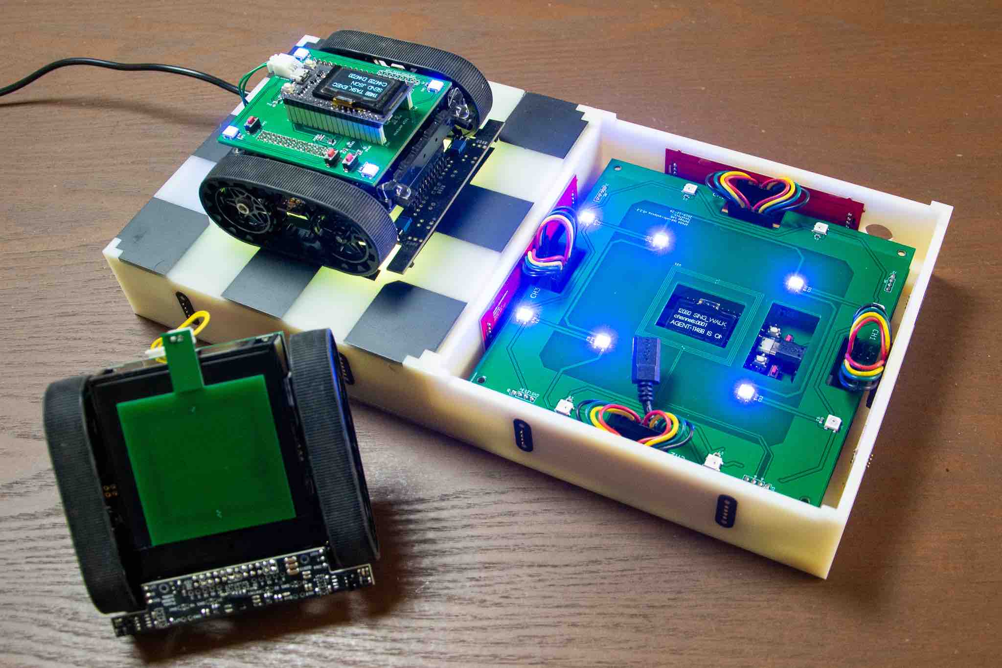
Figure 15: Components of AFADA. The system consists of two kinds of actors: cells and robots. A cell is covered by an acrylic roof patterned for line tracing (left cell), enabling robots to move following the grid structure.

Usage

Robots first receive the OTIMAPP solution from a laptop via Wi-Fi, then move following the plan. Cells achieve mutual exclusion of locations for robots, i.e., collision avoidance, using local communication as follows. Before moving to the next vertex (i.e., cell; denoted as $v_{\mathit{next}}$), a robot first asks the underlying cell $v_{\mathit{current}}$ the availability of $v_{\mathit{next}}$. Then, $v_{\mathit{current}}$ asks $v_{\mathit{next}}$ its status. If $v_{\mathit{next}}$ is reserved by another robot, $v_{\mathit{current}}$ waits a while and asks the status of $v_{\mathit{next}}$ again; otherwise, $v_{\mathit{current}}$ makes $v_{\mathit{next}}$ reserved and notifies the robot to move to $v_{\mathit{next}}$. When the robot reaches $v_{\mathit{next}}$, then the robot releases $v_{\mathit{current}}$ via $v_{\mathit{next}}$. Importantly, there is no central control at runtime. Any actor (robots, cells, and the laptop that sends the plan) has no methods to know the entire configuration. This also means that the system is fully asynchronous as for timing. Furthermore, there is no global communication; robots and cells decide their actions based on information from nearby actors.

named ref

References

- Atzmon et al. [2020a] Dor Atzmon, Roni Stern, Ariel Felner, Nathan R Sturtevant, and Sven Koenig. Probabilistic robust multi-agent path finding. In Proceedings of International Conference on Automated Planning and Scheduling (ICAPS), 2020.
- Atzmon et al. [2020b] Dor Atzmon, Roni Stern, Ariel Felner, Glenn Wagner, Roman Barták, and Neng-Fa Zhou. Robust multi-agent path finding and executing. Journal of Artificial Intelligence Research (JAIR), 2020.
- Barer et al. [2014] Max Barer, Guni Sharon, Roni Stern, and Ariel Felner. Suboptimal variants of the conflict-based search algorithm for the multi-agent pathfinding problem. In Proceedings of Annual Symposium on Combinatorial Search (SOCS), 2014.
- Čáp et al. [2015] Michal Čáp, Peter Novák, Alexander Kleiner, and Martin Seleckỳ. Prioritized planning algorithms for trajectory coordination of multiple mobile robots. IEEE Transactions on Automation Science and Engineering (T-ASE), 2015.
- Coffman et al. [1971] Edward G Coffman, Melanie Elphick, and Arie Shoshani. System deadlocks. ACM Computing Surveys (CSUR), 1971.
- Dresner and Stone [2008] Kurt Dresner and Peter Stone. A multiagent approach to autonomous intersection management. Journal of Artificial Intelligence Research (JAIR), 2008.
- Erdmann and Lozano-Perez [1987] Michael Erdmann and Tomas Lozano-Perez. On multiple moving objects. Algorithmica, 1987.
- Fanti and Zhou [2004] Maria Pia Fanti and MengChu Zhou. Deadlock control methods in automated manufacturing systems. IEEE Transactions on systems, man, and cybernetics-part A: systems and humans, 2004.
- Hönig et al. [2019] Wolfgang Hönig, Scott Kiesel, Andrew Tinka, Joseph W Durham, and Nora Ayanian. Persistent and robust execution of mapf schedules in warehouses. IEEE Robotics and Automation Letters (RA-L), 2019.
- Kameyama et al. [2021] Shota Kameyama, Keisuke Okumura, Yasumasa Tamura, and Xavier Défago. Active modular environment for robot navigation. In Proceedings of IEEE International Conference on Robotics and Automation (ICRA), 2021.
- Knapp [1987] Edgar Knapp. Deadlock detection in distributed databases. ACM Computing Surveys (CSUR), 1987.
- Ma et al. [2017] Hang Ma, TK Satish Kumar, and Sven Koenig. Multi-agent path finding with delay probabilities. In Proceedings of AAAI Conference on Artificial Intelligence (AAAI), 2017.
- Mannucci et al. [2021] Anna Mannucci, Lucia Pallottino, and Federico Pecora. On provably safe and live multirobot coordination with online goal posting. IEEE Transactions on Robotics (T-RO), 2021.
- Mansouri et al. [2019] Masoumeh Mansouri, Bruno Lacerda, Nick Hawes, and Federico Pecora. Multi-robot planning under uncertain travel times and safety constraints. In Proceedings of International Joint Conference on Artificial Intelligence (IJCAI), 2019.
- Nebel [2020] Bernhard Nebel. On the computational complexity of multi-agent pathfinding on directed graphs. In Proceedings of International Conference on Automated Planning and Scheduling (ICAPS), 2020.
- Okumura et al. [2021] Keisuke Okumura, Yasumasa Tamura, and Xavier Défago. Time-independent planning for multiple moving agents. In Proceedings of AAAI Conference on Artificial Intelligence (AAAI), 2021.
- Peltzer et al. [2020] Oriana Peltzer, Kyle Brown, Mac Schwager, Mykel J Kochenderfer, and Martin Sehr. Stt-cbs: A conflict-based search algorithm for multi-agent path finding with stochastic travel times. 2020.
- Robertson and Seymour [1985] Neil Robertson and Paul D Seymour. Disjoint paths—a survey. SIAM Journal on Algebraic Discrete Methods, 1985.
- Sharon et al. [2015] Guni Sharon, Roni Stern, Ariel Felner, and Nathan R Sturtevant. Conflict-based search for optimal multi-agent pathfinding. Artificial Intelligence (AIJ), 2015.
- Silberschatz et al. [2006] Abraham Silberschatz, Peter B Galvin, and Greg Gagne. Operating system concepts. John Wiley & Sons, 2006.
- Silver [2005] David Silver. Cooperative pathfinding. AIIDE, 2005.
- Stern et al. [2019] Roni Stern, Nathan Sturtevant, Ariel Felner, Sven Koenig, Hang Ma, Thayne Walker, Jiaoyang Li, Dor Atzmon, Liron Cohen, TK Kumar, et al. Multi-agent pathfinding: Definitions, variants, and benchmarks. In Proceedings of Annual Symposium on Combinatorial Search (SOCS), 2019.
- Tel [2000] Gerard Tel. Deadlock-free packet switching. In Introduction to distributed algorithms, chapter 5. 2000.
- Van Den Berg et al. [2011] Jur Van Den Berg, Stephen J Guy, Ming Lin, and Dinesh Manocha. Reciprocal n-body collision avoidance. In Robotics Research. 2011.
- Wagner and Choset [2017] Glenn Wagner and Howie Choset. Path planning for multiple agents under uncertainty. In Proceedings of International Conference on Automated Planning and Scheduling (ICAPS), 2017.
- Wurman et al. [2008] Peter R Wurman, Raffaello D’Andrea, and Mick Mountz. Coordinating hundreds of cooperative, autonomous vehicles in warehouses. AI magazine, 2008.
- Zhang et al. [2018] Xu Zhang, Mingyang Li, Jian Hui Lim, Yiwei Weng, Yi Wei Daniel Tay, Hung Pham, and Quang-Cuong Pham. Large-scale 3d printing by a team of mobile robots. Automation in Construction, 2018.