A Majorization Penalty Method for SVM with Sparse Constraint

Abstract

Support vector machine is an important and fundamental technique in machine learning. Soft-margin SVM models have stronger generalization performance compared with the hard-margin SVM. Most existing works use the hinge-loss function which can be regarded as an upper bound of the 0-1 loss function. However, it can not explicitly limit the number of misclassified samples. In this paper, we use the idea of soft-margin SVM and propose a new SVM model with a sparse constraint. Our model can strictly limit the number of misclassified samples, expressing the soft-margin constraint as a sparse constraint. By constructing a majorization function, a majorization penalty method can be used to solve the sparse-constrained optimization problem. We apply Conjugate-Gradient (CG) method to solve the resulting subproblem. Extensive numerical results demonstrate the impressive performance of the proposed majorization penalty method. Support Vector Machine; Majorization Penalty Method; Conjugate Gradient Method; Sparse Constraint.

1 Introduction

Support vector machine (SVM) is a traditional and effective machine learning method [2, 32, 33, 34, 40, 23]. SVM preserves the performance benchmark records of handwritten numerical recognition, text classification, information retrieval and time series prediction. They are usually used for DNA microarray data analysis [1, 22, 34, 40]. Given the training data $x_{1},x_{2},\dots,x_{n}\in{\rm I}\!{\rm R}^{m}$ and the corresponding labels $y_{1},y_{2},\dots,y_{n}\in\{-1,1\}$, SVM is aimed to find a hyperplane $\omega^{T}x+b=0$ to separate the data according to labels, where $\omega\in{\rm I}\!{\rm R}^{m}$ and the bias $b\in{\rm I}\!{\rm R}$ need to be determined. The classical hard-margin SVM is given as follows:

$$\begin{array}[]{ll}\underset{\omega\in{\rm I}\!{\rm R}^{m},b\in{\rm I}\!{\rm R}}{\min}&\frac{1}{2}\|\omega\|^{2}\\ \ \ \ \ \text{s.t.}&y_{i}(\omega^{T}x_{i}+b)\geq 1\ \ \ i=1,2,\dots,n.\end{array}$$ (1)

In the classical SVM, we are looking for $(\omega,b)$ such that the hyperplane $\omega^{T}x+b=0$ can separate the data as much as possible in the sence that the distince between two types of data is maximized. In such situation, data are separated strictly, which is based on the assumption that the data can be linearly separated.

In most cases, optimization methods are designed to solve SVM models with soft margin. Some typical examples are the L1-SVM and L2-SVM models. We will briefly review the methods for the above two models, which are related to our work. For a survey of machine learning optimization methods, please refer to [7, 15]. SVM model with linear summation of the hinge loss is very common, which is called L1-SVM as follows

$$\begin{array}[]{ll}\underset{\omega\in{\rm I}\!{\rm R}^{m},b\in{\rm I}\!{\rm R}}{\min}&\frac{1}{2}\|\omega\|^{2}+\rho\sum\limits_{i=1}^{n}\text{max}(1-y_{i}(\omega^{T}x_{i}+b),0).\\ \end{array}$$ (2)

L1-SVM was put forward by Tibshirani et al. in [47]. For L1-SVM, since the L1 loss function is not differentiable, most algorithms cannot be applied. In [16], Mangasarian used Newton’s method to solve L1-SVM for selecting features from a very high dimensional space. In [27], Mangasarian used a generalized Newton’s method to solve the exact L1-SVM. Hsieh et al. [19] proposed a dual coordinate method (DCD) for the dual problem of L1-SVM. Yan and Li proposed an augmented Lagrangian method for the primal problem of L1-SVM. By using the Moreau-Yosida regularization and the proximal operator, they dealt with the nonsmooth term of L1-SVM very well [36].

If it is the sum of squares of the hinge loss, it is called L2-SVM, as shown below:

$$\begin{array}[]{ll}\underset{\omega\in{\rm I}\!{\rm R}^{m},b\in{\rm I}\!{\rm R}}{\min}&\frac{1}{2}\|\omega\|^{2}+\rho\sum\limits_{i=1}^{n}\text{max}(1-y_{i}(\omega^{T}x_{i}+b),0)^{2}.\\ \end{array}$$ (3)

The relationship and characteristics of the two models were analyzed in details in [8, 13, 30, 31, 35]. For the L2-SVM model, Mangasarian [26] introduced the finite Newton’s method due to the nondifferentiability of the objective function gradient. It is basically a unit-step semismooth Newton’s method, which uses the inverse of Hessian matrix to calculate the Newton’s direction. Keerthi and Decoste [21] proposed an improved Newton’s method. They calculated Newton points and performed an accurate line search to determine the step size, which is suited for large scale data mining tasks. Lin et al. porposed the Trust region Newton method (TRN) [24] for L2-SVM. Chang et al. [9] proposed a coordinate descent method for L2-SVM. They used Newton’s method to solve the subproblem with one variable while fixing other variables. In [19], Hsieh et al. also proposed a dual coordinate descent method (DCD) for the dual problem of L2-SVM with large-scale sparse data. Recently, Hsia et al. [18] studied the trust region updating rule in Newton’s method. Yin and Li proposed a semismooth Newton and achieved remarkable results in [37].

Both L1-SVM and L2-SVM consider the hinge loss function, which is $max(1-y_{i}(\omega^{T}x_{i}+b),0)$. When the sample $(x_{i},y_{i})$ is correctly classified and the functional margin $y_{i}(\omega^{T}x_{i}+b)$ is greater than 1, the loss is 0; otherwise, the loss is $1-y_{i}(\omega^{T}x_{i}+b)$ or $(1-y_{i}(\omega^{T}x_{i}+b))^{2}$. However, the hinge loss function is essentially the surrogate of 0-1 loss function, that is

$$I(1-y_{i}(\omega^{T}x_{i}+b)>0):=\left\{\begin{aligned} 1,&&1-y_{i}(\omega^{T}x_{i}+b)>0,\\ 0,&&\text{otherwise}.\ \ \ \ \ \ \ \ \end{aligned}\right.$$

We give a figure drawing the relationship of L1, L2 and 0-1 loss function in Fig. 1.

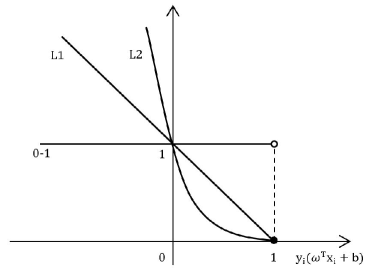
Figure 1: L1, L2 and 0-1 loss function. L1: $\max(0,y_{i}(\omega^{T}x_{i}+b))$; L2: $\max(0,y_{i}(\omega^{T}x_{i}+b))^{2}$; 0-1: $I(1-y_{i}(\omega^{T}x_{i}+b)>0)$.

Because the 0-1 loss function is discontinuous, few algorithms deal with it directly. The above observations motivate us to propose a new model based on 0-1 loss function. The corresponding SVM model with 0-1 loss function is natually presented as

$$\begin{array}[]{ll}\underset{\omega\in{\rm I}\!{\rm R}^{m},b\in{\rm I}\!{\rm R}}{\min}&\frac{1}{2}\|\omega\|^{2}+C\sum\limits_{i=1}^{n}I(1-y_{i}(\omega^{T}x_{i}+b)>0),\\ \end{array}$$ (4)

where $C>0$ is a regularization parameter. For sample data $i\in\{1,\dots,n\}$, the soft-margin model expects that the sample is correctly classified, i.e., $1-y_{i}(\omega^{T}x_{i}+b)\leq 0$, despite a few of them may be misclassified. In other words, for a very few of $i\in\{1,2,\dots,n\}$, there is $1-y_{i}(\omega^{T}x_{i}+b)>0$. Let $s$ $(\gg n)$ be a parameter denoting the upper bound of the number of samples that can not be classified correctly. Then we can reach the following model

$$\begin{array}[]{ll}\underset{\omega\in{\rm I}\!{\rm R}^{m},b\in{\rm I}\!{\rm R}}{\min}&\frac{1}{2}\|\omega\|^{2}\\ \ \ \ \ \text{s.t.}&\sum\limits_{i=1}^{n}I(1-y_{i}(\omega^{T}x_{i}+b)>0)\leq s.\end{array}$$ (5)

Denote $z=[z_{1},z_{2},\dots,z_{n}]^{T}\in{\rm I}\!{\rm R}^{n}$ by $z_{i}=1-y_{i}(\omega^{T}x_{i}+b)$. Model (5) can be written as the following SVM with a sparse constraint

$$\begin{array}[]{ll}\underset{\omega\in{\rm I}\!{\rm R}^{m},b\in{\rm I}\!{\rm R}}{\min}&\frac{1}{2}\|\omega\|^{2}\\ \ \ \ \ \text{s.t.}&\|z_{+}\|_{0}\leq s,\\ &z_{i}=1-y_{i}(\omega^{T}x_{i}+b)\ \ \ i=1,2,\dots,n,\end{array}$$ (6)

where $(\cdot)_{+}:=\text{max}(\cdot,0)$ and $\|\cdot\|_{0}$ is the number of non-zero elements in a vector, which is often referred to as 0 norm. When $s=0$, (6) reduces to the hard-margin SVM problem (1).

0 norm in (6) leads to the sparse constrained optimization problem, which is a NP-hard problem. In order to deal with the computing challenges of 0 norm, the current algorithm is mainly divided into two mainstreams [42]. One is ’greedy’, which means a variety of relaxation forms [41, 17, 43]. Another is called ’relaxtion’, which directly deals with the problem of 0 norm. For example, matching pursuit [25] provides a fast and compact method of adaptive function approximation. The orthogonal matching pursuit [11] produces sub-optimal function expansions by iteratively choosing dictionary waveforms. The subspace pursuit [10] has a low computational complexity and deals with very sparse signals. The compressive sampling matching pursuit (CoSaMP) [28] offers rigorous bounds on computational cost and storage. The hard thresholding pursuit (HTP) [14] combines the iterative hard thresholding (IHT) algorithm and CoSaMP. The conjugate gradient iterative hard thresholding [4] combines the low cost of each iteration of the simple line search IHT with the improved convergence speed.

Various traditional methods have been extended to sparse constrained nonlinear optimization. A gradient hard-thresholding method was proposed by Bahmani et al. in [3], which generalizes CoSaMP. Yuan et al. generalized HTP to the sparse constrained convex optimization [39] and proposed a Newton greedy pursuit method [38]. Zhou et al. [46] built the algorithm of Newton Hard-Thresholding Pursuit for the sparse-constrained optimization with the quadratic convergence rate. Blumensath and Davies proposed IHT algorithm for the linear compressed sensing problem in [5, 6]. Based on this, Pan et al. [29] gave an improved iterative hard thresholding algorithm by employing the Armijo-type stepsize rule, which automatically adjusts the stepsize and the support set and leads to a sufficient decrease of the objective function in each iteration.

The inspiration of our paper comes from the framework of majorization projection method in [45]. For solving the Euclidean distance matrix problem with box constraints and rank constraint, it is difficult to deal with the matrix rank constraint. Zhou et al. [45] penalized the quadratic distance function of a point to the conditional positive semidefinite cone with the rank cut. By finding the subgradient of the penalty function, they constructed the majorization function. They also analyzed the convergence of the resulting majorization penalty method. Note that the rank of a matrix and the 0 norm of a vector are both essentially counting functions. This leads us to think about whether we can apply the same technique and extend it to the vector optimization with 0-norm constraint. It is worth noting that there is also work on SVM with 0 norm constraint recently. Zhou established optimality conditions with the stationary equations and solved it by Newton-type method in [44].

Our Contribution. In this paper, we first propose a new SVM model, that is (5), which considers 0-norm constraint directly to restrict the number of misclassified samples no greater than a given level. We consider the subproblem in penalty method and penalize the 0-norm constraint to the objective function. After that, a majorization penalty algorithm framework is proposed, which is also suitable for our SVM model. The subproblem of the resulting algorithm is essentially a strongly convex quadratic programming without constraints and can be efficiently solved by conjugate gradient method. Finally, we present extensive numerical results to show the efficiency of the proposed method.

This article is organized as follows. In Section 2, we discus the penalty method for (6). In Section 3, we will construct the majorization function, and derive the majorization penalty method. In Section 4, we solve the majorization subproblem by CG method. Extensive numerical examples will illustrate the impressive performance of our algorithm in Section 5. Final conclusions are given in Section 6.

Notation. Let $\boldsymbol{1}_{n}\in{\rm I}\!{\rm R}^{n}$ be a vector which all elements are equal to one. For a vector $x\in{\rm I}\!{\rm R}^{n}$, $Diag(x)\in{\rm I}\!{\rm R}^{n\times n}$ is diagonal matrix whose $i$-th diagonal element is $x_{i}$. We use $\|\cdot\|$ to denote the L2 norm of vectors.

2 Penalty Method for SVM with Sparse Constraint (6)

In this section, we consider the penalty method for SVM with sparse constraint (6).

Recall the SVM model with the sparse constraint as in (6). Let $\Omega_{s}$ be the set defined as $\Omega_{s}:=\{x\in{\rm I}\!{\rm R}^{n}\ |\ \|x_{+}\|_{0}\leq s\}$. Then (6) can be equivalently written as follows

$$\begin{array}[]{ll}\underset{\omega\in{\rm I}\!{\rm R}^{m},b\in{\rm I}\!{\rm R}}{\min}&\frac{1}{2}\|\omega\|^{2}\\ \ \ \ \ \text{s.t.}&z_{i}=1-y_{i}(\omega^{T}x_{i}+b),\ \ \ i=1,2,\dots,n,\\ &z\in\Omega_{s}.\end{array}$$ (7)

We call it sparse constrained SVM model (SCSVM), where the sparse constraint set $\Omega_{s}$ is a non-convex set.

For the sparse constrained set $\Omega_{s}$, in order to measure the distance between $z$ and $\Omega_{s}$, define $g:{\rm I}\!{\rm R}^{n}\rightarrow{\rm I}\!{\rm R}$ as

$$g(z)=\frac{1}{2}\text{dist}^{2}(z,\Omega_{s}),$$

where

$$\text{dist}(z,\Omega_{s}):=\min\{\|z-x\|\ |\ x\in\Omega_{s}\}.$$ (8)

Let $\Pi_{\Omega_{s}}^{B}(z)$ be the set of the optimal solutions of (8). Due to the nonconvexity of $\Omega_{s}$, $\Pi_{\Omega_{s}}^{B}(z)$ may contain multiple points. Let $\Pi_{\Omega_{s}}(z)\in\Pi_{\Omega_{s}}^{B}(z)$ be one of the elements in $\Pi_{\Omega_{s}}^{B}(z)$. Then

$$g(z)=\frac{1}{2}\|z-\Pi_{\Omega_{s}}(z)\|^{2}.$$ (9)

Therefore, $z\in\Omega_{s}$ is equivalent to $g(z)=0$. Model (7) is equivalent to

$$\begin{array}[]{ll}\underset{\omega\in{\rm I}\!{\rm R}^{m},b\in{\rm I}\!{\rm R}}{\min}&\frac{1}{2}\|\omega\|^{2}\\ \ \ \ \ \text{s.t.}&z_{i}=1-y_{i}(\omega^{T}x_{i}+b),\ \ \ i=1,2,\dots,n,\\ &g(z)=0.\end{array}$$ (10)

Due to the equivalence between (7) and (10), (10) is a nonconvex problem and it is in general NP hard. Inspired by [45], we consider the penalty method to solve (10) which penalizes the nonconvex constraint $g(z)=0$. The subproblem in the penalty method is reformulated as

$$\begin{array}[]{ll}\underset{\omega\in{\rm I}\!{\rm R}^{m},b\in{\rm I}\!{\rm R}}{\min}&F_{\rho}(\omega,b):=\frac{1}{2}\|\omega\|^{2}+\rho g(z)\\ \ \ \ \ \text{s.t.}&z_{i}=1-y_{i}(\omega^{T}x_{i}+b),\ \ \ i=1,2,\dots,n,\end{array}$$ (11)

where $\rho>0$ is a penalty parameter.

Denote

$$A=[x_{1},x_{2},\dots,x_{n}]^{T}\in{\rm I}\!{\rm R}^{n\times m},P=\begin{bmatrix}I_{m}\ 0\end{bmatrix}\in{\rm I}\!{\rm R}^{m\times(m+1)}\text{ and }Q=\begin{bmatrix}A\ \boldsymbol{1}_{n}\end{bmatrix}\in{\rm I}\!{\rm R}^{n\times(m+1)}$$ (12)

where $n$ is the number of samples and $m$ is the number of features. Moreover, let $\theta\in{\rm I}\!{\rm R}^{m+1}$ be defined as

$$\theta:=\begin{bmatrix}\omega\\ b\end{bmatrix}\in{\rm I}\!{\rm R}^{m+1}.$$

There is

$$\omega=P\theta\text{ and }A\omega+b=Q\theta.$$

The constraints in (11) can be reformulated as

$$z=\boldsymbol{1}_{n}-Diag(y)(A\omega+b)=\boldsymbol{1}_{n}-\bar{Q}\theta,$$ (13)

where $\bar{Q}:=Diag(y)Q\in{\rm I}\!{\rm R}^{n\times(m+1)}$. Therefore, (10) is equivalent to the following problem

$$\begin{array}[]{ll}\underset{\theta\in{\rm I}\!{\rm R}^{m+1}}{\min}&f(\theta)\\ \ \ \ \ \text{s.t.}&p(\theta)=0,\end{array}$$

where

$$f(\theta):=\frac{1}{2}\|P\theta\|^{2}\ \ \text{ and}\ \ \ p(\theta):=g(\boldsymbol{1}_{n}-\bar{Q}\theta).$$ (14)

Similarly, substituting (13) into $F_{\rho}(\omega,b)$ in (11), we get the following equivalent new unconstrained problem of (11)

$$\begin{array}[]{ll}\underset{\theta\in{\rm I}\!{\rm R}^{m+1}}{\min}&F_{\rho}(\theta):=f(\theta)+\rho p(\theta).\end{array}$$ (15)

Now the aim in the penalty method is how we solve the subproblem (15). To apply majorization method, we will first derive the majorization function for $p(\theta)$ in (15), as shown in Section 3.

3 The Majorizaiton Function

For subproblem (15), it is still not easy to solve. The difficulty lies in $p(\cdot)$. Therefore, similar to as that in [45], we would like to construct the majorization function of $p$ in order to apply the majorization method. To that end, we introduce the defination of majorization function. The majorization function $p(\theta)$ at $t\in{\rm I}\!{\rm R}^{m+1}$, denoted as $p_{m}(\theta,t)$, has to satisfy the following conditions

$$p_{m}(t,t)=p(t)\ \ \text{and}\ \ p_{m}(\theta,t)\geq p(\theta)\ \text{for any}\ \theta\in{\rm I}\!{\rm R}^{m+1}.$$ (16)

We first give a theorem saying we can have a general choice of majorization function for the sets which enjoy the orthogonal projection property.

Theorem 3.1

For a closed set $\mathcal{D}$, let $\Pi^{B}_{\mathcal{D}}(\theta)$ denote the set of projections of a vector $\theta$ onto $\mathcal{D}$ and $\Pi_{\mathcal{D}}(\theta)\in\Pi^{B}_{\mathcal{D}}(\theta)$. Let $k(\theta):=\frac{1}{2}\|\Pi_{\mathcal{D}}(\theta)\|^{2}$ and $q(\theta):=\frac{1}{2}\|\theta-\Pi_{\mathcal{D}}(\theta)\|^{2}$. If

• $\langle\Pi_{\mathcal{D}}(\theta),\theta-\Pi_{\mathcal{D}}(\theta)\rangle=0$ for any $\theta$;

• $\Pi_{\mathcal{D}}(\theta)\in\partial k(\theta)$, where $\partial k(\theta)$ denotes the subdifferential of $h$ at $\theta$,

then for a fixed point $t$, $q_{m}(\theta,t)$ defined by

$$q_{m}(\theta,t):=\frac{1}{2}\|\theta\|^{2}-\langle{\Pi_{\mathcal{D}}(\theta)},\theta-t\rangle-k(t)$$

is a majorization function of $q(\theta)$ at $t$.

proof 3.2

By the defination of $q(\theta)$, there is

$$q(\theta) =\frac{1}{2}\|\theta-\Pi_{\mathcal{D}}(\theta)\|^{2}$$

$$=\frac{1}{2}\|\theta\|^{2}+\frac{1}{2}\|\Pi_{\mathcal{D}}(\theta)\|^{2}-\langle\Pi_{\mathcal{D}}(\theta),\theta\rangle$$

$${=\frac{1}{2}\|\theta\|^{2}+\frac{1}{2}\|\Pi_{\mathcal{D}}(\theta)\|^{2}-\langle\Pi_{\mathcal{D}}(\theta),\theta-\Pi_{\mathcal{D}}(\theta)+\Pi_{\mathcal{D}}(\theta)\rangle}$$

$${=\frac{1}{2}\|\theta\|^{2}-\frac{1}{2}\|\Pi_{\mathcal{D}}(\theta)\|^{2}-\langle\Pi_{\mathcal{D}}(\theta),\theta-\Pi_{\mathcal{D}}(\theta)\rangle}$$

$$=\frac{1}{2}\|\theta\|^{2}-{\frac{1}{2}\|\Pi_{\mathcal{D}}(\theta)\|^{2}}\ \ \ \ \ \text{(condition (a))}$$

$$\leq\frac{1}{2}\|\theta\|^{2}-\langle{\Pi_{\mathcal{D}}(\theta)},\theta-t\rangle-k(t)\ \ \ \ \ \text{(condition (b))}$$

$$=q_{m}(\theta,t).$$

Notice that $q_{m}(t,t)=q(t).$ Therefore, $q_{m}(\theta,t)$ is a majorization function of $q(\theta)$ at $t$.

In fact, Theorem 3.1 holds for ${\mathcal{D}}:=\Omega_{s}$. To show this, we first give the characterization of $\Pi^{B}_{\Omega_{s}}(z).$

For convenience, for $z\in{\rm I}\!{\rm R}^{n}$, we use $z^{\downarrow}\in{\rm I}\!{\rm R}^{n}$ to denote the vector whose elements come from $z$ and are arranged in a descending order. That is, $z^{\downarrow}_{1}\geq z^{\downarrow}_{2}\geq\dots\geq z^{\downarrow}_{n}.$ Define

$$\alpha=\{i\ |\ z_{i}>z^{\downarrow}_{s}\text{ and }z_{i}>0\},\ \ \beta=\{i\ |\ z_{i}=z^{\downarrow}_{s}\text{ and }z_{i}>0\},$$ (17)

$$\gamma=\{i\ |\ 0<z_{i}<z^{\downarrow}_{s}\}\text{ and }\tau=\{i\ |\ z_{i}\leq 0\}.$$ (18)

Let $\Pi^{B}_{\Omega_{s}}(z)$ denote the set of projections of $z$ onto $\Omega_{s}$. Then we give the computation of $\Pi^{B}_{\Omega_{s}}(z)$ for $z\in{\rm I}\!{\rm R}^{n}$ as follows.

Proposition 3.3

For any $z\in{\rm I}\!{\rm R}^{n}$, there is

$$\begin{array}[]{ll}\Pi^{B}_{\Omega_{s}}(z)=\{x\ |&\ x_{i}=z_{i}\ for\ i\in\alpha\cup\beta_{1}{\cup\tau},\ x_{i}=0\ for\ i\in(\beta\backslash\beta_{1})\cup\gamma,\\ &where\ \beta_{1}\subset\beta\ and\ |\beta_{1}|=s-|\alpha|\}.\end{array}$$ (19)

proof 3.4

Projecting $z$ to the set $\Omega_{s}$ is equivalent to projecting $max(z,0)$ to the set $\{x\in{\rm I}\!{\rm R}^{n}\ |\ \|x\|_{0}\leq s\}$. That is, one needs to keep the largest $s$ components of $max(z,0)$ the same and make the others zero. Note that the negative part of $z$ has no effect on the projection. To sum up, the projection of $z$ to $\Omega_{s}$ remains components in $\alpha\cup\beta_{1}\cup\tau$, the other components are 0. Therefore, we get (3.3). The proof is finished.

Due to Proposition 3.3, we have the following results.

Proposition 3.5

Let $\Pi_{\Omega_{s}}(z)\in\Pi^{B}_{\Omega_{s}}(z)$. Define $h(\theta):=\frac{1}{2}\|\Pi_{\Omega_{s}}(\boldsymbol{1}_{n}-\bar{Q}\theta)\|^{2}.$ For a given vector $\tilde{\theta}\in{\rm I}\!{\rm R}^{n+1}$, we have

• $\langle\Pi_{\Omega_{s}}(z),z-\Pi_{\Omega_{s}}(z)\rangle=0$ for any $z{\in{\rm I}\!{\rm R}^{n}}$;

• $-\bar{Q}^{T}\Pi_{\Omega_{s}}({\boldsymbol{1}_{n}-{\bar{Q}}\tilde{\theta}})\in\partial h(\tilde{\theta})$;

proof 3.6

For (i), we first show the following holds

$$(\Pi_{\Omega_{s}}(z))_{i}(z-\Pi_{\Omega_{s}}(z))_{i}=0,\ i=1,2,\dots,n.$$ (20)

If $(\Pi_{\Omega_{s}}(z))_{i}=0$, it is obvious that $(\Pi_{\Omega_{s}}(z))_{i}(z-\Pi_{\Omega_{s}}(z))_{i}=0$. If $(\Pi_{\Omega_{s}}(z))_{i}\neq 0$, by Proposition 3.3, then $i\in\alpha\cup\beta_{1}{\cup\tau}$. Therefore, $(\Pi_{\Omega_{s}}(z))_{i}=z_{i}$. So $z-\Pi_{\Omega_{s}}(z)_{i}=0$ giving again $(\Pi_{\Omega_{s}}(z))_{i}(z-\Pi_{\Omega_{s}}(z))_{i}=0$. Therefore, (20) holds. To sum up, we have $\langle\Pi_{\Omega_{s}}(z),z-\Pi_{\Omega_{s}}(z)\rangle=0$.

For (ii), it is equivalent to the following inequality ( letting $\tilde{z}=\boldsymbol{1}_{n}-\bar{Q}\tilde{\theta}$)

$$h(\theta)-h(\tilde{\theta})\geq\langle-\bar{Q}^{T}\Pi_{\Omega_{s}}(\tilde{z}),\theta-\tilde{\theta}\rangle,\forall\ \theta\in{\rm I}\!{\rm R}^{m+1}.$$ (21)

Note that

$$\langle-\bar{Q}^{T}\Pi_{\Omega_{s}}(\tilde{z}),\theta-\tilde{\theta}\rangle$$

$$= -\langle\Pi_{\Omega_{s}}(\tilde{z}),\bar{Q}(\theta-\tilde{\theta})\rangle$$

$$= -\langle\Pi_{\Omega_{s}}(\tilde{z}),\bar{Q}\theta\rangle+\langle\Pi_{\Omega_{s}}(\tilde{z}),\bar{Q}\tilde{\theta}\rangle$$

$$= -\langle\Pi_{\Omega_{s}}(\tilde{z}),\bar{Q}\theta\rangle+\langle\Pi_{\Omega_{s}}(\tilde{z}),\boldsymbol{1}_{n}\rangle+\langle\Pi_{\Omega_{s}}(\tilde{z}),\bar{Q}\tilde{\theta}-\boldsymbol{1}_{n}\rangle$$

$$= -\langle\Pi_{\Omega_{s}}(\tilde{z}),\bar{Q}\theta-\boldsymbol{1}_{n}\rangle-\langle\Pi_{\Omega_{s}}(\tilde{z}),\tilde{z}\rangle\ \ \ \text{(by $\tilde{z}=\boldsymbol{1}_{n}-\bar{Q}\tilde{\theta}$)}$$

$$= \langle\Pi_{\Omega_{s}}(\tilde{z}),z\rangle-\|\Pi_{\Omega_{s}}(\tilde{z})\|^{2}\ \ \text{(condition (i) and $z=\boldsymbol{1}_{n}-\bar{Q}\theta$)}$$

$$= \langle\Pi_{\Omega_{s}}(\tilde{z}),z\rangle-2h(\tilde{\theta}).$$

So (21) is equivalent to the following conditions:

$$h(\theta)+h(\tilde{\theta})\geq\langle\Pi_{\Omega_{s}}(\tilde{z}),z\rangle,\ {\forall\ \theta\in{\rm I}\!{\rm R}^{m+1}\text{ and }z=\boldsymbol{1}_{n}-\bar{Q}\theta}.$$ (22)

To show (22), due to the definition of $\Pi_{\Omega_{s}}(z)$, we have

$$\|\Pi_{\Omega_{s}}(z)-z\|^{2}\leq\|\Pi_{\Omega_{s}}(\tilde{z})-z\|^{2},\ {\forall\ z\in{\rm I}\!{\rm R}^{n}},$$

which is equivalent to

$$\|\Pi_{\Omega_{s}}(z)\|^{2}-2\langle\Pi_{\Omega_{s}}(z),z\rangle\leq\|\Pi_{\Omega_{s}}(\tilde{z})\|^{2}-2\langle\Pi_{\Omega_{s}}(\tilde{z}),z\rangle.$$

By (i), we have $\langle\Pi_{\Omega_{s}}(z),z\rangle=\|\Pi_{\Omega_{s}}(z)\|^{2}$. Bringing it to the above inequality, we get

$$-\|\Pi_{\Omega_{s}}(z)\|^{2}\leq\|\Pi_{\Omega_{s}}(\tilde{z})\|^{2}-2\langle\Pi_{\Omega_{s}}(\tilde{z}),z\rangle.$$

Rearranging the above in equality gives (22). The proof is complete.

Remark 3.7

Theorem 3.1 and Proposition 3.5 provide us with a method to construct the majorizaiton funtion of $p(\theta)$ in (14). For fixed $\tilde{\theta}\in{\rm I}\!{\rm R}^{m+1}$ and any $\theta\in{\rm I}\!{\rm R}^{m+1}$, we have

$$p(\theta) =g(z)$$

$$=\frac{1}{2}\|z-\Pi_{\Omega_{s}}(z)\|^{2}$$

$$=\frac{1}{2}\|z\|^{2}+\frac{1}{2}\|\Pi_{\Omega_{s}}(z)\|^{2}-\langle\Pi_{\Omega_{s}}(z),z\rangle$$

$$=\frac{1}{2}\|z\|^{2}-h(\theta)\ \ \ \ \ \ \text{(Proposition \ref{corollary1.2} (i))}$$

$$\leq\frac{1}{2}\|\boldsymbol{1}_{n}-\bar{Q}\theta\|^{2}-h(\tilde{\theta})+\langle\bar{Q}^{T}\Pi_{\Omega_{s}}({\boldsymbol{1}_{n}-\bar{Q}\tilde{\theta}}),\theta-\tilde{\theta}\rangle$$

(Proposition 3.5 (ii))

$$=:p_{m}(\theta,\tilde{\theta}).$$

Therefore, $p_{m}(\theta,\tilde{\theta})$ is a majorization function of $p(\theta)$ at $\tilde{\theta}$.

4 Majorization Penalty Method

4.1 Algorithm of Majorization Penalty Method (MPM)

Having introduced the majorizaiton function of $p(\theta)$, we are ready to persent the majorizaiton penalty method. The idea of majorization penalty method is to solve the penalty problem (15) by solving the majorization problem. That is, at iteration $\theta^{k}$, we solve the following subproblem

$$\begin{array}[]{ll}\underset{\theta\in{\rm I}\!{\rm R}^{m+1}}{\min}&F_{k}(\theta):=\frac{1}{2}\|P\theta\|^{2}+\rho p_{m}(\theta,\theta^{k}).\end{array}$$ (23)

The details of majorization penalty method for solving problem (6) is given in Algorithm 4.1.

Algorithm 4.1

(MPM method for (6))

• Input: data matrix $A\in{\rm I}\!{\rm R}^{n\times m}$, sparse threshold $s>0$, the initial $\theta^{0}{\in{\rm I}\!{\rm R}^{m+1}}$ and the penalty parameter $\rho>0$. Set $k=0$.

• Solve subproblem (23) to get a solution $\theta^{k+1}$.

• If it reaches the stopping criterion, stop; otherwise $k:=k+1$ and go to S2.

Next, we mainly discuss the convergence of Algorithm 4.1. The idea of this proof is basically the same as Themrem 3.7 in [45]. Due to the majorization strategy, there is

$$F_{\rho}(\theta^{k}) =f(\theta^{k})+\rho p(\theta^{k})$$

$$=f(\theta^{k})+\rho p_{m}(\theta^{k},\theta^{k})$$

$$\geq f(\theta^{k+1})+\rho p_{m}(\theta^{k+1},\theta^{k})$$

$$\geq f(\theta^{k+1})+\rho p(\theta^{k+1})$$

$$=F_{\rho}(\theta^{k+1}).$$

As a result, the seqence $\{F_{\rho}(\theta^{k})\}$ generated by Algorithm 4.1 is nonincreasing. Besides, the sequence is bounded below by $0$. Therefore, it converges.

Next, we will give two propositions which will be used later.

Proposition 4.2

For $\rho>0$, $P^{T}P+\rho Q^{T}Q$ is a positive definite matrix.

proof 4.3

For contradiction, assume that $P^{T}P+\rho Q^{T}Q$ is negative semidefinite. There is a nonzero vector $x\in{\rm I}\!{\rm R}^{m+1}$ such that

$$x^{T}(P^{T}P+\rho Q^{T}Q)x\leq 0.$$

Note that

$$P^{T}P=\begin{bmatrix}I_{m}&0\\ 0&0\end{bmatrix}\ \ \text{and}\ \ Q^{T}Q=\begin{bmatrix}A^{T}A&A^{T}\boldsymbol{1}_{n}\\ \boldsymbol{1}_{n}^{T}A&n\end{bmatrix}=\begin{bmatrix}\sum\limits_{i=1}^{n}x_{i}x_{i}^{T}&\sum\limits_{i=1}^{n}x_{i}\\ (\sum\limits_{i=1}^{n}x_{i})^{T}&n\end{bmatrix}.$$ (24)

Therefore, we have

$$x^{T}(P^{T}P+\rho Q^{T}Q)x=\sum_{i=1}^{m}x_{i}^{2}+\rho x^{T}Q^{T}Qx\leq 0.$$

Noticing that $Q^{T}Q$ is a positive semi-definite matrix, the above formula can only be 0. That is $x_{i}=0$ for $i=1,2,\dots,m$ and $x^{T}Q^{T}Qx=0$. On the other hand, we have

$$Qx=\begin{bmatrix}A\ \boldsymbol{1}_{n}\end{bmatrix}\begin{bmatrix}0\\ \vdots\\ 0\\ x_{m+1}\end{bmatrix}=x_{m+1}.$$

We get $x_{m+1}=0$. That is, $x=0$, which is contradictory. Therefore, $P^{T}P+\rho Q^{T}Q$ is positive definite.

We need the following assumption.

Assumption 1. $\tilde{z}\in{\rm I}\!{\rm R}^{n}$ has distinct elements.

Proposition 4.4

Let $\{z_{k}\}$ be a sequence whose limit is $\tilde{z}$, that is, $\underset{k\rightarrow\infty}{\lim}z_{k}=\tilde{z}$. Suppose $\tilde{z}$ satisfies Assumption 1. Then $\underset{k\rightarrow\infty}{\lim}\Pi_{\Omega_{s}}(z_{k})=\Pi_{\Omega_{s}}(\tilde{z})$.

proof 4.5

Because we all components of $\tilde{z}$ are distinct, both $\Pi_{\Omega_{s}}^{B}(z_{k})$ and $\Pi_{\Omega_{s}}^{B}(\tilde{z})$ are singletons. That is, $\Pi^{B}_{\Omega_{s}}(z_{k})=\{\Pi_{\Omega_{s}}(z_{k})\}$ and $\Pi^{B}_{\Omega_{s}}(\tilde{z})=\{\Pi_{\Omega_{s}}(\tilde{z})\}$.

Donate $\alpha(z)$ and $\beta(z)$ as in (17) with respect to $z$. First, we will prove that

$$\alpha(z_{k})\cup\beta(z_{k})=\alpha(\tilde{z})\cup\beta(\tilde{z})$$

when $k$ is large enough. Suppose the above equation does not hold, which means that there is an index $i$ such that $i\in\alpha(z_{k})\cup\beta(z_{k})$ and $i\notin\alpha(\tilde{z})\cup\beta(\tilde{z})$ or an index $j$ such that $j\notin\alpha(z_{k})\cup\beta(z_{k})$ and $j\in\alpha(\tilde{z})\cup\beta(\tilde{z})$. Because $|\alpha(z_{k})\cup\beta(z_{k})|=|\alpha(\tilde{z})\cup\beta(\tilde{z})|=s$, such $i$ and $j$ exist at the same time. Above all, we get two sets of inequalities as follows

$$(z_{k})_{i}\geq(z_{k})_{s}^{\downarrow}>(z_{k})_{j}\ \text{ and }\ (\tilde{z})_{i}<(\tilde{z})_{s}^{\downarrow}\leq(\tilde{z})_{j}.$$

Combined the above formulae with $\underset{k\rightarrow\infty}{\lim}z_{k}=\tilde{z}$ and the order preserving property of sequence limit, it is contradictory. So $\alpha(z_{k})\cup\beta(z_{k})=\alpha(\tilde{z})\cup\beta(\tilde{z})$. Therefore, we get $\underset{k\rightarrow\infty}{\lim}(\Pi_{\Omega_{s}}(z_{k}))_{i}=(\Pi_{\Omega_{s}}(\tilde{z}))_{i}$ for any $i\in\alpha(z_{k})\cup\beta(z_{k})=\alpha(\tilde{z})\cup\beta(\tilde{z})$.

For $i\notin\alpha(\tilde{z})\cup\beta(\tilde{z})$, note that $(\Pi_{\Omega_{s}}(z_{k}))_{i}=min\{(z_{k})_{i},0\}$ and $(\Pi_{\Omega_{s}}(\tilde{z}))_{i}=min\{\tilde{z}_{i},0\}$. Because $min\{\cdot,0\}$ is a continuous monotone increasing function and $\underset{k\rightarrow\infty}{\lim}z_{k}=\tilde{z}$, we get $\underset{k\rightarrow\infty}{\lim}(\Pi_{\Omega_{s}}(z_{k}))_{i}=(\Pi_{\Omega_{s}}(\tilde{z}))_{i}$ for any $i\notin\alpha(z_{k})\cup\beta(z_{k})$.

Therefore, $\underset{k\rightarrow\infty}{\lim}\Pi_{\Omega_{s}}(z_{k})=\Pi_{\Omega_{s}}(\tilde{z})$ holds. The proof is finished.

Based on Proposition 4.2 and Proposition 4.4, we will a give stronger convergence below.

Theorem 4.6

Let $\{\theta^{k}\}$ be the sequence generated by the MPM. We have the following results.

• $F_{\rho}(\theta^{k+1})-F_{\rho}(\theta^{k})\leq-\frac{\rho}{2}\|\theta^{k+1}-\theta^{k}\|^{2},\ k=1,2\dots$. Conseqencetly, $\|\theta^{k+1}-\theta^{k}\|\rightarrow 0.$

• Let $\hat{\theta}$ be an accumulation point of $\{\theta^{k}\}$ and assume that $\hat{z}=\boldsymbol{1}_{n}-\bar{Q}\hat{\theta}$ satisfy Assumption 1. Then for any $\theta$, we have

  $$\langle\nabla f(\hat{\theta})-\rho\bar{Q}^{T}{(\boldsymbol{1}_{n}-\bar{Q}\hat{\theta})}+\rho\bar{Q}\Pi_{\Omega_{s}}(\boldsymbol{1}_{n}-\bar{Q}\hat{\theta}),\theta-\hat{\theta}\rangle\geq 0,$$

  whcih means that $\hat{\theta}$ is a stationary point of (15).

• If $\hat{\theta}$ is an isolated accumulation point of the sequence $\{\theta^{k}\}$, then the whole sequence $\{\theta^{k}\}$ converges to $\hat{\theta}$.

proof 4.7

(i) Let

$$z^{k}:=\boldsymbol{1}_{n}-{\bar{Q}}\theta^{k}\text{ and }z^{k+1}:=\boldsymbol{1}_{n}-{\bar{Q}}\theta^{k+1}.$$ (25)

Note that

$$f(\theta^{k+1})-f(\theta^{k})=\frac{1}{2}\langle P(\theta^{k+1}+\theta^{k}),P(\theta^{k+1}-\theta^{k})\rangle=\frac{1}{2}\langle P^{T}P(\theta^{k+1}+\theta^{k}),\theta^{k+1}-\theta^{k}\rangle$$ (26)

and

$$\nabla f(\theta^{k+1})=P^{T}P\theta^{k+1}.$$ (27)

Moreover, there is

$$\|z^{k+1}\|^{2}-\|z^{k}\|^{2}=2\langle z^{k+1}-z^{k},z^{k+1}\rangle-\|z^{k+1}-z^{k}\|^{2}$$

$$=2\langle\theta^{k+1}-\theta^{k},-\bar{Q}^{T}z^{k+1}\rangle-\|z^{k+1}-z^{k}\|^{2}.$$

By Proposition 3.5 (ii), we have

$$h(\theta^{k+1})-h(\theta^{k})\geq\langle-\bar{Q}^{T}\Pi_{\Omega_{s}}({z^{k}}),\theta^{k+1}-\theta^{k}\rangle.$$ (28)

Since $\theta^{k+1}$ is the optimal solution of (23), by the optimality condition of (23), there is

$$\nabla F_{k}(\theta^{k+1})=0,$$ (29)

where $\nabla F_{k}(\theta^{k+1})=\nabla f(\theta^{k+1})-\rho\bar{Q}^{T}(\boldsymbol{1}_{n}-{\bar{Q}}\theta^{k+1})+\rho\bar{Q}^{T}\Pi_{\Omega_{s}}(z^{k})$.

Therefore,

$$F_{\rho}(\theta^{k+1})-F_{\rho}(\theta^{k})$$

$$= f(\theta^{k+1})-f(\theta^{k})+\rho p(\theta^{k+1})-\rho p(\theta^{k})\ \ (\text{by}(\ref{def_f_g}))$$

$$= \frac{1}{2}\langle P^{T}P(\theta^{k+1}+\theta^{k}),\theta^{k+1}-\theta^{k}\rangle+(\rho/2)(\left\|z^{k+1}\right\|^{2}-\left\|z^{k}\right\|^{2})$$

$$-\rho(h(\theta^{k+1})-h(\theta^{k}))\ \ (\text{by }(\ref{f-f}))$$

$$= \langle\nabla f(\theta^{k+1}),\theta^{k+1}-\theta^{k}\rangle-\frac{1}{2}\langle P^{T}P(\theta^{k+1}-\theta^{k}),\theta^{k+1}-\theta^{k}\rangle$$

$$+ (\rho/2)(\left\|z^{k+1}\right\|^{2}-\left\|z^{k}\right\|^{2})-\rho(h(\theta^{k+1})-h(\theta^{k}))\ \ (\text{by }(\ref{nabla_f}))$$

$$= \left\langle\nabla f(\theta^{k+1})-\rho\bar{Q}z^{k+1},\theta^{k+1}-\theta^{k}\right\rangle-\frac{1}{2}\|P(\theta^{k+1}-\theta^{k})\|^{2}$$

$$-(\rho/2)\left\|z^{k+1}-z^{k}\right\|^{2}-\rho(h(\theta^{k+1})-h(\theta^{k}))\ \ (\text{by }(\ref{convergence_2}))$$

$$\leq \left\langle\nabla f(\theta^{k+1})-\rho\bar{Q}z^{k+1}+\rho\bar{Q}^{T}\Pi_{\Omega_{s}}(z^{k}),\theta^{k+1}-\theta^{k}\right\rangle$$

$$-\frac{1}{2}\|P(\theta^{k+1}-\theta^{k})\|^{2}-(\rho/2)\left\|z^{k+1}-z^{k}\right\|^{2}\ \ (\text{by }(\ref{convergence_3}))$$

$$= -\frac{1}{2}\|P(\theta^{k+1}-\theta^{k})\|^{2}-(\rho/2)\left\|\bar{Q}(\theta^{k+1}-\theta^{k})\right\|^{2}\ \ (\text{by }(\ref{convergence_4}))$$

$$= -\frac{1}{2}\langle(P^{T}P+\rho Q^{T}Q)(\theta^{k+1}-\theta^{k}),\theta^{k+1}-\theta^{k}\rangle.$$

Due to Proposition 4.2, $P^{T}P+\rho Q^{T}Q$ is a positive definite matrix. Let $\lambda_{min}>0$ be the smallest eigenvalue of $P^{T}P+\rho Q^{T}Q.$ There is

$$F_{\rho}(\theta^{k+1})-F_{\rho}(\theta^{k})\leq-\frac{1}{2}\lambda_{min}\|\theta^{k+1}-\theta^{k}\|^{2}.$$

This proves that the sequence $\{F_{\rho}(\theta^{k})\}$ is non-increasing and it is also bounded below by 0. Taking the limits on both sides, we have $\|\theta^{k+1}-\theta^{k}\|^{2}\rightarrow 0$.

(ii) We first prove that $\{\theta_{k}\}$ generated by Algorithm 4.1 is bounded. Because $\{F_{\rho}(\theta^{k})\}$ is non-increasing and it is also bounded below by 0, as proved in (i), $\{F_{\rho}(\theta^{k})\}$ is bounded. Therefore, we have

$$F_{\rho}(\theta^{k})=\frac{1}{2}\|\omega_{k}\|^{2}+\frac{\rho}{2}\|z_{k}-\Pi_{\Omega_{s}}(z_{k})\|^{2}\geq\frac{1}{2}\|\omega_{k}\|^{2},$$

which shows that both $\{\omega_{k}\}$ and $\{\|z_{k}-\Pi_{\Omega_{s}}(z_{k})\|\}$ are bounded. The latter means that for any index $i\in(\beta(z_{k})\ \backslash\beta_{1}(z_{k}))\cup\gamma(z_{k})$, there is $\{(z_{k})_{i}\}$ is bounded, which leads to the boundness of $\{(z_{k})_{i}\}$. Note that $(z_{k})_{i}=1-y_{i}(\omega_{k}^{T}x_{i}+b_{k})$, which means that $b_{k}$ is bounded. So we proved that $\{\theta_{k}\}$ is bounded.

Therefore, we suppose $\hat{\theta}$ is the limit of a subsequence, denoted by $\{\theta^{k_{l}}\}$. Due to $\|\theta^{k+1}-\theta^{k}\|^{2}\rightarrow 0$ in (i), we get the sequence $\{\theta^{k_{l}+1}\}$ also converges to $\hat{\theta}$. Since $\theta^{k+1}$ is the optimal solution of (23), by the optimality condition of (23), there is

$$\nabla F_{k}(\theta^{k+1})^{T}(\theta-\theta^{k+1})\geq 0,$$

That is,

$$\langle\nabla f(\theta^{k+1})-\rho Q^{T}z^{k+1}+\rho Q^{T}\Pi_{\Omega_{s}}(z^{k}),\theta-\theta^{k+1}\rangle\geq 0.$$ (30)

Due to Proposition 4.4, we can take the limit for both sides of (30) and get

$$\langle\nabla f(\hat{\theta})-\rho\bar{Q}^{T}(\boldsymbol{1}_{n}-\bar{Q}\hat{\theta})+\rho\bar{Q}\Pi_{\Omega_{s}}(\boldsymbol{1}_{n}-\bar{Q}\hat{\theta}),\theta-\hat{\theta}\rangle\geq 0.$$

Therefore, $\hat{\theta}$ is a stationary point of (15).

(iii) We have proved $\|\theta^{k+1}-\theta^{k}\|\rightarrow 0$ in (i). From Theorem 5.4 in [20], the whole sequence converges to $\hat{\theta}$.

4.2 Solving Subproblem (23)

In (23), the function $F_{k}(\theta)$ can be simplified as

$$F_{k}(\theta) =\frac{1}{2}\|P\theta\|^{2}+\frac{\rho}{2}\|\boldsymbol{1}_{n}-\bar{Q}\theta\|^{2}+\rho\langle\Pi_{\Omega_{s}}(\boldsymbol{1}_{n}-\bar{Q}\theta^{k}),\bar{Q}(\theta-\theta^{k})\rangle-\rho h(\theta^{k})$$

$$=\frac{1}{2}\|P\theta\|^{2}+\frac{\rho}{2}\|\boldsymbol{1}_{n}-\bar{Q}\theta\|^{2}+\rho\langle\Pi_{\Omega_{s}}(\boldsymbol{1}_{n}-\bar{Q}\theta^{k}),\bar{Q}\theta\rangle+C_{0}$$

$$=\frac{1}{2}\|P\theta\|^{2}+\frac{\rho}{2}\|\bar{Q}\theta\|^{2}+\rho\langle\Pi_{\Omega_{s}}(\boldsymbol{1}_{n}-\bar{Q}\theta^{k})-\boldsymbol{1}_{n},\bar{Q}\theta\rangle+C_{1}$$

$$=\frac{1}{2}\|P\theta\|^{2}+\frac{\rho}{2}\|\bar{Q}\theta\|^{2}+\rho\langle\bar{Q}^{T}\Pi_{\Omega_{s}}(\boldsymbol{1}_{n}-\bar{Q}\theta^{k})-\boldsymbol{1}_{n},\theta\rangle+C_{1},$$

where $C_{0}=\rho\langle\Pi_{\Omega_{s}}(\boldsymbol{1}_{n}-\bar{Q}\theta^{k}),\bar{Q}\theta^{k}\rangle-\rho h(\theta^{k}$) and $C_{1}=C_{0}+\frac{\rho}{2}\|\boldsymbol{1}_{n}\|^{2}$ denote the constant parts with respect to $\theta$.

Notice that $F_{k}(\theta)$ is a convex function, solving (23) is equivalent to solve

$$\nabla F_{k}(\theta)=0,$$ (31)

where

$$\nabla F_{k}(\theta)=(P^{T}P+\rho Q^{T}Q)\theta+\rho\bar{Q}^{T}(\Pi_{\Omega_{s}}(\boldsymbol{1}_{n}-\bar{Q}\theta^{k})-\boldsymbol{1}_{n}).$$

Equation (31) can be regarded as

$$(P^{T}P+\rho Q^{T}Q)\theta=\rho\bar{Q}^{T}(\boldsymbol{1}_{n}-\Pi_{\Omega_{s}}(\boldsymbol{1}_{n}-\bar{Q}\theta^{k})),$$ (32)

where $P^{T}P$ and $Q^{T}Q$ are defiend as in (24).

Note that by Proposition 4.2, $P^{T}P+\rho Q^{T}Q$ is a positive definite matrix, which actually shows that (23) is an unconstrained strongly convex quadratic programming problem. It ensures that solving (32) is meaningful and one will get an unique optimal solution of (23).

To sum up, in majorization penalty method MPM, solving each subproblem (23) reduces to solving a linear system (31), which has a symmetric positive definite coefficient matrix. To further speed up the algorithm, below we discuss more details about solving (31) more efficiently.

Remark 4.8

For (31), when $m$ is small ($m<100$), we can compute the inverse of a matrix directly. That means, we solve the linear system (23) by direct solver. In other cases, We use conjugate gradient method, which is an iterative solver and is suitable for solving large-scale linear systems.

5 Numberical Experiment and Comparsion

In this section, we first discuss the performance of our algorithm with different choices of parameters. Then we will compare it with the state-of-art algorithms provided by LIBLINEAR in [12].

All experiments are tested in Matlab R2016b in Windows 10 on a Lenovo desktop computer with an Intel(R) Core(TM) i5-9300H CPU at 2.40 GHZ and 16 GB of RAM.

For the stopping criterion, similar to that in [45], we define two residuals to measure the convergence of $f$ and $p$ respectively. That is,

$$\texttt{f-prog}_{k}:=\frac{f(\theta^{k-1})-f(\theta^{k})}{\rho+f(\theta^{k-1})}$$

and

$$\texttt{p-prog}_{k}: =\frac{2p(\theta^{k})}{\|\theta^{k}\|^{2}}=\frac{2g(\boldsymbol{1}_{n}-\bar{Q}\theta^{k})}{\|\theta^{k}\|^{2}}.$$

The smaller $\texttt{p-prog}_{k}$ means that $z$ is closer to $\Omega_{s}$ in (7). MPM stops when the following conditions hold

$$\texttt{f-prog}_{k}\leq\sqrt{n}10^{-3}\ \text{and}\ \texttt{p-prog}_{k}\leq 10^{-3}.$$

5.1 Performance of Our Algorithm

In this part, we use LIBLINEAR’s standard real data set for classification ($38$ data sets). For some classification data sets whose labels do not belong to $\{-1,1\}$, we change their labels and set them to belong to $\{-1,1\}$. For example, for the dataset ”breast-cancer”, the label of the sample is $2$ or $4$. We turn tag $2$ into $1$ and tag $4$ into $1$. Similarly, we use the same strategy for the dataset: ”liver-disease”, ”mushrooms”, ”phishing” and ”svmguide1”. The detailed information of classification data sets is shown in Table 1.

Table 1: Data Information for Classification ($n$ is the number of instances, $m$ is the number of features, $\#$nonzeros represents the number of non-zero elements in all training instances and density shows the ratio: $\#$nonzeros/(m·n)).

Data set	n	m	$\#$nonzeros	density
a1a	30956	123	429343	11.28$\%$
a2a	30296	123	420188	11.28$\%$
a3a	29376	123	407430	11.28$\%$
a4a	27780	123	385302	11.28$\%$
a5a	26147	123	362653	11.28$\%$
a6a	21341	123	295984	11.28$\%$
a7a	16461	123	228288	11.28$\%$
a8a	22696	123	314815	11.28$\%$
a9a	32561	123	451592	11.28$\%$
w1a	47272	300	551176	3.89$\%$
w2a	46279	300	539213	3.89$\%$
w3a	44837	300	522338	3.89$\%$
w4a	42383	300	493583	3.89$\%$
w5a	39861	300	464466	3.89$\%$
w6a	32561	300	379116	3.89$\%$
w7a	25057	300	291438	3.89$\%$
w8a	49749	300	579586	3.89$\%$
australian	690	14	8447	87.44$\%$
breast-cancer	638	10	6380	100$\%$
cod-rna	59535	8	476280	100$\%$
colon-cancer	62	2000	124000	100$\%$
diabetes	768	8	6135	99.85$\%$
duke breast-cancer	38	7129	270902	100$\%$
fourclass	862	2	1717	99.59$\%$
german.numer	1000	24	23001	95.84$\%$
heart	270	13	3510	100$\%$
ijcnn1	49990	22	649870	59.09$\%$
ionosphere	351	34	10551	88.41$\%$
leukemia	38	7129	270902	100$\%$
liver-disorders	145	5	725	100$\%$
mushrooms	8124	112	170604	18.75$\%$
phishing	11055	68	331610	44.11$\%$
skin nonskin	245057	3	735171	100$\%$
splice	2175	60	130500	100$\%$
sonar	208	60	12479	99.99$\%$
svmguide1	3089	4	12356	100$\%$
svmguide3	1243	22	27208	99.50$\%$
covtype.binary	581012	54	6940438	22.12$\%$

We choose the parameters as follows: the initial penalty parameter $\rho=0.4$ in Algorithm 1 Step 3, the initial point $\theta^{0}=0$, maximum iteration number of CG method is $500$. The CG method is stopped if the residual in CG is smaller than $10^{-3}$. We report the number of iterations $k$, the total number of CG iterations $cg$, the cputime $t$ and the accuracy of the algorithm with different sparse ratios $SR$, where the accuracy is calculated by

$$\frac{\text{number of test data whose predicted labels are correct}}{\text{number of test {data}}}$$

and the sparse ratio $SR$ can be calculated with

$$SR:=\frac{s}{n}\times 100\%.$$

In Table 2 and Table 3, we use ${}^{\prime}0^{\prime}$ to indicate that we did not use CG method in this case.

From Table 2 and Table 3, we get the following conclusions: (i) The algorithm has solved all the problems successfully. This shows that our method can solve the problem (7) in a short cuptime. (ii) When the $SR$ is very high (such as $50\%$), the cputime $t$, the total number of CG iterations $cg$ and the number of majorization iterations $k$ are lower than other cases. This is because when the $SR$ is very high, it can be regarded as we no longer considering the sparse constraint, and the algorithm can converge faster. In other words, when the $SR$ is very high, the convergence criterion is easier to achieve. (iii) From the result of accuracy, the same data set has different solutions with different $SR$s. It is difficult to find a suitable $SR$ for all data sets. In the following numerical experiments, we set $SR$ to $10\%$.

Table 2: Numerical Results for MPM with Different Sparse Ratio (I).

data set	$SR$	k	$cg$	t(s)	accuracy	data set	$SR$	k	$cg$	t(s)	accuracy
a1a	1$\%$	17	1061	0.545	84.1775$\%$	a2a	1$\%$	16	1152	0.027	84.3346$\%$
	5$\%$	24	1486	0.035	83.7253$\%$		5$\%$	22	1596	0.035	84.1827$\%$
	10$\%$	27	1699	0.037	83.4992$\%$		10$\%$	25	1811	0.040	84.1926$\%$
	15$\%$	23	1409	0.034	83.5024$\%$		15$\%$	23	1668	0.038	84.0045$\%$
	25$\%$	21	1303	0.032	80.4917$\%$		25$\%$	16	1203	0.025	81.4266$\%$
	50$\%$	11	729	0.017	83.2730$\%$		50$\%$	11	836	0.018	83.4599$\%$
a3a	1$\%$	18	1487	0.035	84.3239$\%$	a4a	1$\%$	19	1791	0.052	84.4888$\%$
	5$\%$	25	2056	0.049	84.1435$\%$		5$\%$	25	2420	0.061	84.4240$\%$
	10$\%$	25	2083	0.043	83.7078$\%$		10$\%$	26	2574	0.059	84.3269$\%$
	15$\%$	24	1970	0.041	83.2755$\%$		15$\%$	26	2603	0.060	83.5421$\%$
	25$\%$	17	1437	0.030	80.4739$\%$		25$\%$	18	1858	0.048	81.3139$\%$
	50$\%$	11	976	0.023	83.2006$\%$		50$\%$	12	1255	0.034	83.8013$\%$
a5a	1$\%$	20	2129	0.054	84.5642$\%$	a6a	1$\%$	19	2451	0.078	84.7383$\%$
	5$\%$	25	2701	0.071	84.5298$\%$		5$\%$	25	3208	0.097	84.7196$\%$
	10$\%$	27	2912	0.067	84.3653$\%$		10$\%$	26	3358	0.113	84.5368$\%$
	15$\%$	25	2732	0.064	83.7763$\%$		15$\%$	24	3085	0.097	83.3372$\%$
	25$\%$	18	2034	0.053	80.8965$\%$		25$\%$	20	2632	0.088	79.4574$\%$
	50$\%$	12	1297	0.035	83.4551$\%$		50$\%$	12	1576	0.062	83.6652$\%$
a7a	1$\%$	19	2712	0.097	84.9098$\%$	a8a	1$\%$	19	2850	0.120	85.3421$\%$
	5$\%$	25	3527	0.124	84.9341$\%$		5$\%$	26	3990	0.149	85.1698$\%$
	10$\%$	26	3678	0.131	84.7640$\%$		10$\%$	27	4127	0.157	85.2712$\%$
	15$\%$	25	3575	0.121	83.7191$\%$		15$\%$	29	4485	0.171	83.7304$\%$
	25$\%$	16	2361	0.085	80.9611$\%$		25$\%$	18	2790	0.109	79.9088$\%$
	50$\%$	11	1586	0.066	83.4639$\%$		50$\%$	11	1658	0.076	84.1257$\%$
a9a	1$\%$	19	3269	0.153	85.0378$\%$	w1a	1$\%$	25	1177	0.045	96.8668$\%$
	5$\%$	25	4247	0.197	84.8658$\%$		5$\%$	8	436	0.019	95.1873$\%$
	10$\%$	27	4591	0.196	84.7307$\%$		10$\%$	10	524	0.022	95.1736$\%$
	15$\%$	25	4252	0.185	83.5821$\%$		15$\%$	10	525	0.022	95.1668$\%$
	25$\%$	17	2911	0.141	78.9755$\%$		25$\%$	9	483	0.021	93.7370$\%$
	50$\%$	12	2005	0.117	83.2320$\%$		50$\%$	14	711	0.030	93.2718$\%$
w2a	1$\%$	32	4404	0.282	98.2889$\%$	w3a	1$\%$	31	1018	0.036	97.7519$\%$
	5$\%$	9	1530	0.124	96.8660$\%$		5$\%$	14	551	0.020	97.6894$\%$
	10$\%$	7	1200	0.113	95.9926$\%$		10$\%$	14	586	0.021	97.5110$\%$
	15$\%$	9	1473	0.120	96.0847$\%$		15$\%$	9	377	0.015	97.0738$\%$
	25$\%$	9	1530	0.127	95.4965$\%$		25$\%$	8	318	0.013	96.9200$\%$
	50$\%$	9	1572	0.130	92.9418$\%$		50$\%$	10	392	0.016	96.4784$\%$
w4a	1$\%$	28	2051	0.096	97.1965$\%$	w5a	1$\%$	23	2096	0.105	98.4697$\%$
	5$\%$	7	654	0.037	94.7947$\%$		5$\%$	8	879	0.057	96.9820$\%$
	10$\%$	8	719	0.040	94.7660$\%$		10$\%$	9	949	0.058	96.9695$\%$
	15$\%$	10	869	0.047	94.6635$\%$		15$\%$	10	1048	0.066	96.9619$\%$
	25$\%$	8	722	0.048	92.6756$\%$		25$\%$	8	867	0.055	95.7026$\%$
	50$\%$	12	1006	0.052	91.6510$\%$		50$\%$	12	1202	0.071	94.9023$\%$
w6a	1$\%$	24	2712	0.165	98.3624$\%$	w7a	1$\%$	23	3138	0.193	98.6750$\%$
	5$\%$	7	959	0.073	96.3828$\%$		5$\%$	7	1144	0.096	97.0707$\%$
	10$\%$	8	1057	0.077	96.3980$\%$		10$\%$	9	1404	0.104	97.0627$\%$
	15$\%$	9	1199	0.085	96.3714$\%$		15$\%$	11	1653	0.116	97.0348$\%$
	25$\%$	9	1154	0.085	94.8060$\%$		25$\%$	9	1422	0.111	95.6579$\%$
	50$\%$	12	1477	0.106	93.9169$\%$		50$\%$	12	1820	0.135	94.8597$\%$
w8a	1$\%$	25	4586	0.350	98.6222$\%$	australian	1$\%$	20	1071	0.020	83.4025$\%$
	5$\%$	6	1346	0.160	97.0236$\%$		5$\%$	25	1305	0.023	83.6100$\%$
	10$\%$	9	1892	0.187	97.0303$\%$		10$\%$	23	1257	0.022	83.6100$\%$
	15$\%$	10	2084	0.201	96.9701$\%$		15$\%$	21	984	0.017	82.7801$\%$
	25$\%$	9	1918	0.192	95.6725$\%$		25$\%$	16	923	0.017	80.7054$\%$
	50$\%$	12	2467	0.227	95.0505$\%$		50$\%$	11	648	0.012	85.2697$\%$

Table 3: Numerical Results for MPM with Different Sparse Ratio (II).

data set	$SR$	k	$cg$	t(s)	accuracy	data set	$SR$	k	$cg$	t(s)	accuracy
breast-cancer	1$\%$	27	0	0.031	99.5122$\%$	cod-rna	1$\%$	23	0	0.074	60.7133$\%$
	5$\%$	25	0	0.001	99.5122$\%$		5$\%$	24	0	0.079	64.5037$\%$
	10$\%$	18	0	0.001	100.0000$\%$		10$\%$	22	0	0.073	64.7444$\%$
	15$\%$	15	0	0.001	99.5122$\%$		15$\%$	20	0	0.068	64.4701$\%$
	25$\%$	13	0	0.001	98.5366$\%$		25$\%$	16	0	0.060	62.0570$\%$
	50$\%$	10	0	0.001	99.0244$\%$		50$\%$	11	0	0.051	46.6379$\%$
colon-cancer	1$\%$	23	0	0.198	73.6842$\%$	diabetes	1$\%$	4	0	0.002	78.3550$\%$
	5$\%$	3	0	0.183	63.1579$\%$		5$\%$	7	0	0.001	78.7879$\%$
	10$\%$	3	0	0.183	63.1579$\%$		10$\%$	11	0	0.001	77.4892$\%$
	15$\%$	3	0	0.181	57.8947$\%$		15$\%$	16	0	0.001	77.0563$\%$
	25$\%$	3	0	0.180	57.8947$\%$		25$\%$	15	0	0.001	77.0563$\%$
	50$\%$	3	0	0.182	42.1053$\%$		50$\%$	14	0	0.001	67.5325$\%$
duke breast-cancer	1$\%$	25	0	2.273	100.0000$\%$	fourclass	1$\%$	5	0	0.001	75.2896$\%$
	5$\%$	3	0	2.274	100.0000$\%$		5$\%$	11	0	0.001	76.4479$\%$
	10$\%$	3	0	2.348	100.0000$\%$		10$\%$	18	0	0.001	77.2201$\%$
	15$\%$	3	0	2.456	100.0000$\%$		15$\%$	22	0	0.005	76.0618$\%$
	25$\%$	3	0	2.473	100.0000$\%$		25$\%$	24	0	0.002	74.9035$\%$
	50$\%$	3	0	2.447	50.0000$\%$		50$\%$	11	0	0.001	72.2008$\%$
german.numer	1$\%$	5	0	0.002	80.0000$\%$	heart	1$\%$	6	0	0.001	87.6543$\%$
	5$\%$	10	0	0.004	80.0000$\%$		5$\%$	14	0	0.001	86.4198$\%$
	10$\%$	16	0	0.004	79.0000$\%$		10$\%$	17	0	0.003	86.4198$\%$
	15$\%$	21	0	0.004	76.0000$\%$		15$\%$	18	0	0.002	82.7160$\%$
	25$\%$	19	0	0.004	77.0000$\%$		25$\%$	14	0	0.001	87.6543$\%$
	50$\%$	13	0	0.004	73.0000$\%$		50$\%$	12	0	0.001	86.4198$\%$
ijcnn1	1$\%$	31	0	0.171	91.9565$\%$	ionosphere	1$\%$	23	0	0.003	95.2830$\%$
	5$\%$	30	0	0.184	91.7515$\%$		5$\%$	21	0	0.003	95.2830$\%$
	10$\%$	10	0	0.100	90.4996$\%$		10$\%$	20	0	0.002	98.1132$\%$
	15$\%$	11	0	0.106	90.5083$\%$		15$\%$	17	0	0.002	97.1698$\%$
	25$\%$	11	0	0.106	90.5137$\%$		25$\%$	13	0	0.002	97.1698$\%$
	50$\%$	14	0	0.114	87.9761$\%$		50$\%$	10	0	0.002	98.1132$\%$
leukemia	1$\%$	36	0	2.265	64.7059$\%$	liver-disorders	1$\%$	4	0	0.000	50.0000$\%$
	5$\%$	3	0	2.236	64.7059$\%$		5$\%$	6	0	0.000	50.0000$\%$
	10$\%$	3	0	2.255	61.7647$\%$		10$\%$	8	0	0.000	50.0000$\%$
	15$\%$	3	0	2.240	76.4706$\%$		15$\%$	9	0	0.000	50.0000$\%$
	25$\%$	3	0	2.242	82.3529$\%$		25$\%$	11	0	0.001	50.0000$\%$
	50$\%$	2	0	2.218	79.4118$\%$		50$\%$	16	0	0.001	50.0000$\%$
mushrooms	1$\%$	25	767	0.013	100.0000$\%$	phishing	1$\%$	23	0	0.054	91.2270$\%$
	5$\%$	18	569	0.010	100.0000$\%$		5$\%$	23	0	0.051	92.0711$\%$
	10$\%$	14	494	0.008	100.0000$\%$		10$\%$	13	0	0.043	89.3579$\%$
	15$\%$	15	535	0.010	100.0000$\%$		15$\%$	11	0	0.041	88.9358$\%$
	25$\%$	14	562	0.010	100.0000$\%$		25$\%$	11	0	0.045	89.4784$\%$
	50$\%$	12	429	0.013	99.3590$\%$		50$\%$	12	0	0.046	90.4432$\%$
splice	1$\%$	12	0	0.009	64.0920$\%$	spnar	1$\%$	22	0	0.004	17.4603$\%$
	5$\%$	24	0	0.011	62.2989$\%$		5$\%$	21	0	0.002	23.8095$\%$
	10$\%$	25	0	0.010	68.8276$\%$		10$\%$	18	0	0.002	31.7460$\%$
	15$\%$	22	0	0.011	71.6322$\%$		15$\%$	20	0	0.002	25.3968$\%$
	25$\%$	20	0	0.011	64.5057$\%$		25$\%$	13	0	0.002	31.7460$\%$
	50$\%$	13	0	0.009	50.2069$\%$		50$\%$	14	0	0.002	33.3333$\%$
svmguide1	1$\%$	29	0	0.007	95.2750$\%$	svmguide3	1$\%$	8	0	0.003	43.9024$\%$
	5$\%$	28	0	0.007	93.9250$\%$		5$\%$	13	0	0.005	48.7805$\%$
	10$\%$	26	0	0.006	92.1750$\%$		10$\%$	13	0	0.004	43.9024$\%$
	15$\%$	24	0	0.006	90.3000$\%$		15$\%$	13	0	0.004	34.1463$\%$
	25$\%$	21	0	0.006	88.7000$\%$		25$\%$	10	0	0.003	2.4390$\%$
	50$\%$	11	0	0.003	74.9000$\%$		50$\%$	13	0	0.004	60.9756$\%$

5.2 Numerical Comparisions with LIBLINEAR

In this part, we compare our algorithm with some solvers in LIBLINEAR [12]. LIBLINEAR is an open source library for large-scale linear classification. We choose the dual coordinate descent method (DCD) in [19] and the trust-region Newton (TRN) in [24]. DCD is designed for the dual problem of L1-SVM and L2-SVM. TRN is used for the primal from of L2-SVM.

For our MPM, the parameters are consistent as in Section 5.1. We set the $SR$ as $10\%$. For DCD and TRN, all parameters are set as default. We report the cputime and accuracy for each algorithm in Table 4.

Table 4: The Comparison Results. A1: MPM; A2: DCD for dual L2-SVM; A3: TRN for primal L2-SVM; A4: DCD for dual L1-SVM.

data set	t(s) (A1$|$A2$|$A3$|$A4)	accuracy (A1$|$A2$|$A3$|$A4)
a1a	0.029$|$0.040$|$0.002$|$0.004	83.50$|$83.84$|$83.85$|$83.81
a2a	0.033$|$0.012$|$0.003$|$0.006	84.19$|$84.00$|$84.04$|$84.28
a3a	0.042$|$0.018$|$0.003$|$0.008	83.71$|$84.26$|$84.32$|$84.29
a4a	0.059$|$0.028$|$0.005$|$0.016	84.33$|$84.41$|$84.40$|$84.49
a5a	0.066$|$0.039$|$0.008$|$0.020	84.37$|$84.52$|$84.51$|$84.38
a6a	0.094$|$0.076$|$0.013$|$0.037	84.54$|$84.80$|$84.79$|$84.66
a7a	0.119$|$0.115$|$0.021$|$0.060	84.76$|$85.04$|$85.01$|$84.85
a8a	0.148$|$0.187$|$0.031$|$0.119	85.27$|$85.44$|$85.38$|$85.10
a9a	0.228$|$0.315$|$0.041$|$0.142	84.73$|$84.99$|$84.99$|$85.00
w1a	0.024$|$0.003$|$0.002$|$0.002	95.17$|$95.98$|$95.94$|$96.00
w2a	0.105$|$0.214$|$0.032$|$0.062	95.99$|$97.95$|$97.96$|$98.00
w3a	0.023$|$0.003$|$0.001$|$0.001	97.51$|$94.78$|$94.66$|$93.99
w4a	0.037$|$0.016$|$0.007$|$0.006	94.77$|$96.77$|$96.76$|$96.70
w5a	0.057$|$0.033$|$0.010$|$0.014	96.97$|$97.96$|$97.95$|$97.95
w6a	0.075$|$0.096$|$0.019$|$0.023	96.40$|$97.88$|$97.87$|$97.83
w7a	0.106$|$0.129$|$0.026$|$0.046	97.06$|$98.19$|$98.17$|$98.18
w8a	0.190$|$0.438$|$0.060$|$0.100	97.03$|$98.34$|$98.37$|$98.39
australian	0.023$|$0.005$|$0.002$|$0.003	83.61$|$83.40$|$83.20$|$83.20
breast-cancer	0.003$|$0.001$|$0.000$|$0.000	100.00$|$99.51$|$99.51$|$99.51
cod-rna	0.073$|$2.867$|$0.027$|$2.929	64.74$|$47.84$|$58.21$|$48.03
colon-cancer	0.186$|$0.003$|$0.003$|$0.003	63.16$|$68.42$|$68.42$|$68.42
diabetes	0.003$|$0.001$|$0.000$|$0.001	77.49$|$79.22$|$79.22$|$77.49
duke breast-cancer	2.250$|$0.013$|$0.015$|$0.014	100.00$|$100.00$|$100.00$|$100.00
fourclass	0.003$|$0.001$|$0.000$|$0.001	77.22$|$65.25$|$65.64$|$69.11
german.numer	0.005$|$0.008$|$0.001$|$0.003	79.00$|$79.33$|$79.67$|$79.00
heart	0.001$|$0.001$|$0.000$|$0.000	86.42$|$83.95$|$83.95$|$83.95
ijcnn1	0.100$|$0.123$|$0.062$|$0.082	90.50$|$91.79$|$91.78$|$92.11
ionosphere	0.005$|$0.003$|$0.001$|$0.001	98.11$|$98.11$|$98.11$|$99.06
leukemia	2.272$|$0.011$|$0.014$|$0.011	61.76$|$79.41$|$79.41$|$79.41
liver-disorders	0.001$|$0.000$|$0.000$|$0.000	50.00$|$50.00$|$50.00$|$50.00
mushrooms	0.011$|$0.001$|$0.001$|$0.001	100.00$|$100.00$|$100.00$|$100.00
phishing	0.044$|$0.015$|$0.015$|$0.012	89.36$|$91.59$|$91.59$|$91.62
splice	0.011$|$0.055$|$0.003$|$0.014	68.83$|$52.05$|$52.09$|$57.56
spnar	0.004$|$0.002$|$0.001$|$0.002	31.75$|$11.11$|$11.11$|$11.11
svmguide1	0.006$|$0.103$|$0.001$|$0.111	92.17$|$78.55$|$78.92$|$62.65
svmguide3	0.003$|$0.009$|$0.002$|$0.003	43.90$|$24.39$|$24.39$|$9.76

The results obtained in Table 4 are analyzed as follows. The four methods provide good accuracy for most the data sets. For most of the data sets, more than 70$\%$, or even 90$\%$ of the test data can be correctly predicted with right labels. But for some very difficult data sets, our algorithm has a very good result. That is, there is significant improvement in accuracy for solving cod-rna, fourclass, splice, spnar, svmguide1 and svmguide3 (indicated by bold font in Table 4). However, when the feature dimension $m$ of the individual data set is much larger than the sample number $n$ ( colon-cancer, duke breast-cancer and leukemia indicated by underline), MPM takes a bit more time. This can be explained by the fact that the resulting subproblem is a $m$ by $m$ linear system, which takes relatively more time to solve than other data sets.

6 Conclusions

In our paper, we proposed our SCSVM model with 0-norm constraint, which is different from L1-SVM and L2-SVM. We penalized the sparse constraint to the objective function and used the majorizaiton method to solve it approximately. It should be noted that our method itself is not limited to our SVM model. We proposed Theorem 3.1 to deal with more general cases, which shows that as long as conditions (a) and (b) are satisfied, we can apply the majorization penalty method.

The subproblem in the majorization penalty method admits a special form, which is a strongly convex quadratic problem. Therefore, it is equivalent to solving a linear system. We proved the nonsingularity of the Jacobian matrix, and then we used conjugate gradient method to solve the linear equation. In the numerical experiments, we compared with two methods DCD and TRN for models L1-SVM and L2-SVM respectively in LIBLINEAR. The results verified the efficiency of the proposed model and our algorithm.

References

- [1] Hisham Al-Mubaid and Syed A Umair. A new text categorization technique using distributional clustering and learning logic. IEEE Transactions on Knowledge and Data Engineering, 18(9):1156–1165, 2006.
- [2] Mariette Awad and Rahul Khanna. Support vector regression. Efficient learning machines, pages 67–80, 2015.
- [3] Sohail Bahmani, Bhiksha Raj, and Petros T Boufounos. Greedy sparsity-constrained optimization. Journal of Machine Learning Research, 14(Mar):807–841, 2013.
- [4] Jeffrey D Blanchard, Jared Tanner, and Ke Wei. Conjugate gradient iterative hard thresholding: Observed noise stability for compressed sensing. IEEE Transactions on Signal Processing, 63(2):528–537, 2014.
- [5] Thomas Blumensath and Mike E Davies. Iterative thresholding for sparse approximations. Journal of Fourier analysis and Applications, 14(5-6):629–654, 2008.
- [6] Thomas Blumensath and Mike E Davies. Iterative hard thresholding for compressed sensing. Applied and computational harmonic analysis, 27(3):265–274, 2009.
- [7] Léon Bottou, Frank E Curtis, and Jorge Nocedal. Optimization methods for large-scale machine learning. Siam Review, 60(2):223–311, 2018.
- [8] Christopher J Burges and David Crisp. Uniqueness of the svm solution. Advances in neural information processing systems, 12:223–229, 1999.
- [9] Kai-Wei Chang, Cho-Jui Hsieh, and Chih-Jen Lin. Coordinate descent method for large-scale l2-loss linear support vector machines. Journal of Machine Learning Research, 9(Jul):1369–1398, 2008.
- [10] Wei Dai and Olgica Milenkovic. Subspace pursuit for compressive sensing signal reconstruction. IEEE transactions on Information Theory, 55(5):2230–2249, 2009.
- [11] Geoff Davis, Stephane Mallat, and Marco Avellaneda. Adaptive greedy approximations. Constructive approximation, 13(1):57–98, 1997.
- [12] Rong-En Fan, Kai-Wei Chang, Cho-Jui Hsieh, Xiang-Rui Wang, and Chih-Jen Lin. Liblinear: A library for large linear classification. the Journal of machine Learning research, 9:1871–1874, 2008.
- [13] Rodrigo Fernández. Behavior of the weights of a support vector machine as a function of the regularization parameter c. International Conference on Artificial Neural Networks, pages 917–922, 1998.
- [14] Simon Foucart. Hard thresholding pursuit: an algorithm for compressive sensing. SIAM Journal on Numerical Analysis, 49(6):2543–2563, 2011.
- [15] Jerome Friedman, Trevor Hastie, and Robert Tibshirani. The elements of statistical learning, volume 1. Springer series in statistics New York, 2001.
- [16] Glenn M Fung and Olvi L Mangasarian. A feature selection newton method for support vector machine classification. Computational optimization and applications, 28(2):185–202, 2004.
- [17] Jun-ya Gotoh, Akiko Takeda, and Katsuya Tono. Dc formulations and algorithms for sparse optimization problems. Mathematical Programming, 169(1):141–176, 2018.
- [18] Chih-Yang Hsia, Ya Zhu, and Chih-Jen Lin. A study on trust region update rules in newton methods for large-scale linear classification. Asian conference on machine learning, pages 33–48, 2017.
- [19] Cho-Jui Hsieh, Kai-Wei Chang, Chih-Jen Lin, S Sathiya Keerthi, and Sellamanickam Sundararajan. A dual coordinate descent method for large-scale linear svm. Proceedings of the 25th international conference on Machine learning, pages 408–415, 2008.
- [20] Christian Kanzow and Hou-Duo Qi. A qp-free constrained newton-type method for variational inequality problems. Mathematical Programming, 85(1):81–106, 1999.
- [21] S Sathiya Keerthi and Dennis DeCoste. A modified finite newton method for fast solution of large scale linear svms. Journal of Machine Learning Research, 6(Mar):341–361, 2005.
- [22] Kai Labusch, Erhardt Barth, and Thomas Martinetz. Simple method for high-performance digit recognition based on sparse coding. IEEE transactions on neural networks, 19(11):1985–1989, 2008.
- [23] Yuh-Jye Lee and Olvi L Mangasarian. Ssvm: A smooth support vector machine for classification. Computational optimization and Applications, 20(1):5–22, 2001.
- [24] Chih-Jen Lin, Ruby C Weng, and S Sathiya Keerthi. Trust region newton methods for large-scale logistic regression. Proceedings of the 24th international conference on Machine learning, pages 561–568, 2007.
- [25] Stéphane G Mallat and Zhifeng Zhang. Matching pursuits with time-frequency dictionaries. IEEE Transactions on signal processing, 41(12):3397–3415, 1993.
- [26] Olvi L Mangasarian. A finite newton method for classification. Optimization Methods and Software, 17(5):913–929, 2002.
- [27] Olvi L Mangasarian. Exact 1-norm support vector machines via unconstrained convex differentiable minimization. Journal of Machine Learning Research, 7(Jul):1517–1530, 2006.
- [28] Deanna Needell and Joel A Tropp. Cosamp: Iterative signal recovery from incomplete and inaccurate samples. Applied and computational harmonic analysis, 26(3):301–321, 2009.
- [29] Lili Pan, Shenglong Zhou, and Houduo Qi. A convergent iterative hard thresholding for sparsity and nonnegativity constrained optimization. Pacific Journal of Optimization, 13(2):325–353, 2017.
- [30] Massimiliano Pontil and Alessandro Verri. Properties of support vector machines. Neural Computation, 10(4):955–974, 1998.
- [31] Ryan Rifkin, Massimiliano Pontil, and Alessandro Verri. A note on support vector machine degeneracy. International Conference on Algorithmic Learning Theory, pages 252–263, 1999.
- [32] Vladimir Vapnik. Estimation of dependences based on empirical data. Springer Science & Business Media, 2006.
- [33] Vladimir Vapnik. The nature of statistical learning theory. Springer science & business media, 2013.
- [34] Vladimir Vapnik, Steven Golowich, and Alex Smola. Support vector method for function approximation, regression estimation and signal processing. Advances in neural information processing systems, 9:281–287, 1996.
- [35] Hiroyasu Yamada and Yuji Matsumoto. Statistical dependency analysis with support vector machines. Proceedings of the Eighth International Conference on Parsing Technologies, pages 195–206, 2003.
- [36] Yinqiao Yan and Qingna Li. An efficient augmented lagrangian method for support vector machine. Optimization Methods and Software, pages 1–29, 2020.
- [37] Juan Yin and Qingna Li. A semismooth newton method for support vector classification and regression. Computational Optimization and Applications, 73(2):477–508, 2019.
- [38] Xiao-Tong Yuan and Qingshan Liu. Newton greedy pursuit: A quadratic approximation method for sparsity-constrained optimization. Proceedings of the IEEE Conference on Computer Vision and Pattern Recognition, pages 4122–4129, 2014.
- [39] Xiaotong Yuan, Ping Li, and Tong Zhang. Gradient hard thresholding pursuit for sparsity-constrained optimization. International Conference on Machine Learning, pages 127–135, 2014.
- [40] YuBo Yuan and TingZhu Huang. A polynomial smooth support vector machine for classification. International Conference on Advanced Data Mining and Applications, pages 157–164, 2005.
- [41] Cun-Hui Zhang et al. Nearly unbiased variable selection under minimax concave penalty. The Annals of statistics, 38(2):894–942, 2010.
- [42] Chen Zhao, Naihua Xiu, Hou-Duo Qi, and Ziyan Luo. A lagrange-newton algorithm for sparse nonlinear programming. arXiv preprint arXiv:2004.13257, 2020.
- [43] Yun-Bin Zhao. Rsp-based analysis for sparsest and least l1-norm solutions to underdetermined linear systems. IEEE Transactions on Signal Processing, 61(22):5777–5788, 2013.
- [44] Shenglong Zhou. Sparse svm for sufficient data reduction. arXiv e-prints, pages arXiv–2005, 2020.
- [45] Shenglong Zhou, Naihua Xiu, and Hou-Duo Qi. A fast matrix majorization-projection method for penalized stress minimization with box constraints. IEEE Transactions on Signal Processing, 66(16):4331–4346, 2018.
- [46] Shenglong Zhou, Naihua Xiu, and Hou-Duo Qi. Global and quadratic convergence of newton hard-thresholding pursuit. arXiv preprint arXiv:1901.02763, 2019.
- [47] Ji Zhu, Saharon Rosset, Robert Tibshirani, and Trevor Hastie. 1-norm support vector machines. Advances in neural information processing systems, 16:49–56, 2003.