Trimmed Match Design for Randomized Paired Geo Experiments

Abstract.

How to measure the incremental Return On Ad Spend (iROAS) is a fundamental problem for the online advertising industry. A standard modern tool is to run randomized geo experiments, where experimental units are non-overlapping ad-targetable geographical areas (Vaver and Koehler, 2011). However, how to design a reliable and cost-effective geo experiment can be complicated, for example: 1) the number of geos is often small, 2) the response metric (e.g. revenue) across geos can be very heavy-tailed due to geo heterogeneity, and furthermore 3) the response metric can vary dramatically over time. To address these issues, we propose a robust nonparametric method for the design, called Trimmed Match Design (TMD), which extends the idea of Trimmed Match (Chen and Au, 2019) and furthermore integrates the techniques of optimal subset pairing and sample splitting in a novel and systematic manner. Some simulation and real case studies are presented. We also point out a few open problems for future research.

1. Introduction

How to measure the causal effect of online advertising (e.g. on search, display, video) is a fundamental problem, not only important to advertisers but also to ad platforms such as Google and Facebook. Despite lots of research based on observational studies, see Varian (2016) for a recent review, and Sapp et al. (2017), Chen et al. (2018) and references therein for some recent innovations, randomized controlled experiments, as the gold standard for causal inference (Imbens and Rubin, 2015), are preferred in order to get unbiased and trustful measurements. Two kinds of randomized experiments have been proposed: cookie-level experiments, where a large number of cookies are randomly assigned to two different ad serving conditions (treatment and control), and geo experiments, where experimental units are non-overlapping ad-targetable geographical areas, see Adwords (2021) for a list of “geo targets” supported by Google. While a cookie experiment is relatively easier to analyze due to large sample (Johnson et al., 2017; Gordon et al., 2019; Kohavi et al., 2020), it is mostly used for online metrics (e.g., online conversion) and its measurement may be inaccurate due to technical issues such as cross-devices, sign-in/out, cookie churn, etc (Yen et al. (2012) and Coey and Bailey (2016)). More importantly, such experiments may be impossible to execute properly due to data protection laws (e.g. GDPR (2021) in Europe) and due to increasing restrictions on internet user data collection, e.g. removal of third-party cookies from web browsers, see recent updates from Apple (2021) and Google (2021).

To overcome these issues, geo experiments, first proposed by Vaver and Koehler (2011), only require collecting the response metric (e.g., revenue) and ad spend at the geo level, which is an easy task for advertisers and is free of privacy concerns as there is no need to collect any user data. Consequently, randomized geo experiments have become increasingly more popular as they provide a more rigorous tool for measuring ad effectiveness.

However, geo experiments come with their own challenges. In order to minimize the spillover effect due to travel across the boundaries of geos, each geo must be large enough so as to be reasonably isolated from other geos, which often results in: 1) only a small number of geos available for experimentation (Rolnick et al., 2019), and 2) heavy-tailed experimental data. Despite randomness in geo assignment, geo heterogeneity can make it hard to obtain a balanced treatment and control split especially when the sample size is also small. The situation can be further complicated by temporal dynamics (e.g., marketing promotions, a hurricane, covid-19 pandemic)—the split may be balanced earlier but less so later on, even before the experiment starts. Often there exists budget constraints (e.g. total ad spend on geos in the treatment group may be pre-specified, but spends for individual geos are determined by ad platforms through dynamic auction) which introduces dependencies on the measurements across geos and violates the independence assumption made by most statistical models. Lastly, the baseline response for a geo can be a few orders of magnitude larger than the cookie-level response while the number of geos is very small relative to the number of cookies, therefore, in order to detect the same level of incremental effect, geo experiments can be much more expensive than cookie experiments.

In this paper we consider the design problem regarding randomized geo experiments, specifically with a matched paired design. The parameter of interest is the incremental return on ad spend (iROAS), denoted as $\theta$, which is the ratio of overall incremental sales to overall incremental ad spend. Let $\mathcal{G}$ be the set of geos in the population, and for any geo $g\in\mathcal{G}$, let $R_{g}^{T}$ and $R_{g}^{C}$ be the potential responses for the geo under the two ad serving conditions, namely treatment ($T$) and control ($C$), respectively, and similarly define $S_{g}^{T}$ and $S_{g}^{C}$ as potential ad spends. Then the iROAS $\theta$ can be formally expressed as below:

$$\theta =\frac{\sum_{g\in\mathcal{G}}(R_{g}^{T}-R_{g}^{C})}{\sum_{g\in\mathcal{G}}(S_{g}^{T}-S_{g}^{C})}$$

where the numerator is the overall incremental response and the denominator is the overall incremental ad spend, but none of them is directly observable.

The primary purpose of the experiment is to estimate $\theta$. With a proper design, though the actual value of $\theta$ is unknown, we hope to have a good control of the precision of the estimate before the experiment is actually run. We follow the hypothesis testing framework:

(1.1) $$H_{0}:\theta=0 \text{ vs }H_{1}:\theta\geq\theta_{0},$$

where $\theta_{0}$ is a user-specified minimum detectable iROAS. Given a fixed budget, how shall we come up with a matched paired design (i.e. a set of paired geos randomly assigned to treatment and control) so that the experiment data to be collected later would have the capability to accept $H_{0}$ correctly (when $H_{0}$ holds) and accept $H_{1}$ correctly (when $H_{1}$ holds), both with high probabilities, given the challenges mentioned earlier?

Let $N$ be the total number of geos available for experimentation. Let $R_{g}(t)$ and $S_{g}(t)$ be the observed response and ad spend values respectively, for geo $g\in\{1,\cdots,N\}$ at time $t$, where $t$ is usually a day or a week. In some scenarios, the spend value may not exist (e.g. for new advertisers) before the experiment starts, then $S_{g}(t)$ may be some proxy (e.g. population size) to inform the relative level of spend across geos. Both $R_{g}(t)$ and $S_{g}(t)$ are collected prior to the design, referred to as the pretest data hereafter.

We follow the classical advice (Tukey (1993)): balance what you can, randomize the rest, adjust for the random imbalance (that is, rerandomization), analyze by planned and balanced double randomization. As usual, the design procedure here requires the construction of candidate sets of geo pairs, as well as power evaluation for each candidate design, see for example Rosenbaum (2020). However, to the best of our knowledge, there has not been much research specific to measuring the ratio of two causal effects such as iROAS yet, see Chen and Au (2019) and references therein. Our major contributions include: formulation of the design problem under a nonparametric iROAS model, and proposal of the use of Trimmed Match and cross validation (a technique commonly used in model fitting and machine learning, but not for experimental design yet) for robust power analysis. Unlike classical optimal design criteria based on parametric models (Wu and Hamada (2020); Box et al. (2005)) or Taguchi’s robust parameter design (Nair et al., 1992), by using Trimmed Match and cross validation (CV), our method is nonparametric and robust against both geo heterogeneity and temporal dynamics. By cross validation, we split the pretest data into two non-overlapping time periods, where one is used for constructing matched pairs and the other for power analysis. If the same data is used for both pairing and power analysis, it can lead to overestimating the power of the design due to overfitting.

The rest of the paper is organized as follows: Section 2 provides some background on geo experiments, and Section 3 describes the iROAS model and derives a criteria for optimal pairing. The design method is proposed in Section 4. Section 5 reports some numerical studies as well as performance comparison with the design based on standard permutation test. A real case study is reported in Section 6 and Section 7 concludes with some discussions and open problems.

Trimmed Match Design has been applied for customer studies at Google. The implementation code in Python is partially available at GitHub (Chen et al., 2020).

2. Background

To design and analyze randomized geo experiments, Vaver and Koehler (2011) proposed a two-stage regression model, called geo-based regression (GBR), where the first stage fits a weighted linear regression to estimate incremental ad spend, and the second stage fits another weighted linear regression for the response based on estimated incremental spend as well as data prior to the experiment. GBR provides a way to model the iROAS directly and the design can be constructed based on the variance analysis of the estimator. However, the model is sensitive to the choice of the regression weights and thus is not robust against geo heterogeneity, and furthermore, incremental ad spend may correlate with the residual, despite randomness in the treatment assignment, which may bias the estimate (Chen and Au, 2019).

To conquer the geo heterogeneity issue, (Kerman et al., 2017) proposed a time-based regression (TBR) by aggregating the geo-level data into the group level (treatment vs control), which may be treated as a simplified version of the Bayesian structural time series model developed by Brodersen et al. (2015). TBR belongs to the class of synthetic control models and requires some untestable assumptions, despite randomness in geo assignment. Later, based on the TBR model, Au (2018) proposed a market matching method for designing geo experiments by maximizing a linear relationship between two time series responses, one for treatment and the other for control, which requires very few geos (essentially a single pair of grouped geos) and can be less costly if the TBR model fits and predicts well. However, the design method only applies to non-randomized experiments and does not meet the gold standard for causal inference.

Recently Chen and Au (2019) have proposed a sound statistical framework for measuring iROAS based on a randomized paired geo experiment and further developed a robust estimation method, namely Trimmed Match, which will be described in more details in the next section.

There are also some work regarding how to use both geo-level and cookie-level data (Ye et al., 2016) and geo construction through geographical clustering (Rolnick et al., 2019), which are less relevant to this paper.

3. Criteria for Optimal Pairing

In this section, we first describe the iROAS model for a randomized paired design and then derive a criteria for optimal pairing.

3.1. The iROAS model

To draw statistical inference of iROAS $\theta$, we adopt the nonparametric iROAS model proposed by Chen and Au (2019), which assumes that iROAS $\theta$ is the same across geos, an assumption first proposed by Vaver and Koehler (2011). Given a randomized design with $n$ pairs of geos, let $Y_{i}$ $(X_{i})$ be the response difference (spend difference) between the treatment geo and the control geo in the $i$th pair during the experiment period, for $i=1,\cdots,n$. Then the model can be stated as follows:

(3.1) $$Y_{i} =\theta\cdot X_{i}+\epsilon_{i},\text{ where }\epsilon_{i}\text{ is symmetric around 0.}$$

Here $X_{i}$ is random. Note that $\epsilon_{i}$ may be correlated with $X_{i}$, which makes the above model different from traditional linear models. The main statistical obstacle comes from the fact that despite symmetry, the distribution of $\{\epsilon_{i}:i=1,\cdots,n\}$ can be very heavy-tailed due to geo heterogeneity.

To illustrate the basic idea behind the model, with some abuse of notation, let $(R_{ij},S_{ij})$ be the response and spend during the test period for the $j$th geo in the $i$th pair, where $j\in\{1,2\}$ and $i\in\{1,\cdots,n\}$, and let

(3.2) $$Z_{ij} =R_{ij}-\theta S_{ij}$$

which represents the “uninfluenced” response in the sense that the effect due to ad spend has been subtracted. Then if $\theta$ is the true iROAS for each geo, the $Z$ value for a specific geo would be the same no matter whether that geo would be treated or controlled (see Lemma 1 of Chen and Au (2019)).

Let $A_{i}$ indicate the random assignment for the $i$th pair with $P(A_{i}=1)=P(A_{i}=-1)=1/2$ , where $A_{i}=1$ indicates that the first geo is assigned to treatment and the second geo to control, while $A_{i}=-1$ indicates the opposite assignment. By definition we can rewrite $Y_{i}=A_{i}\cdot(R_{i1}-R_{i2})$ and $X_{i}=A_{i}\cdot(S_{i1}-S_{i2})$, then the symmetric distribution of $\epsilon_{i}$ in model (3.1) follows from the fact that

(3.3) $$Y_{i}-\theta X_{i} \equiv A_{i}\cdot(Z_{i1}-Z_{i2})$$

where both $Z_{i1}$ and $Z_{i2}$ are invariant to geo assignment.

3.2. Criteria for optimal pairing

To estimate $\theta$, we adopt the robust method “Trimmed Match” (Chen and Au, 2019), which can be described as follows. Since $\epsilon_{i}(\theta)\equiv Y_{i}-\theta\cdot X_{i}$ follows a symmetric distribution around 0 at the true $\theta$ value, the Trimmed Match estimator $\hat{\theta}$ solves the trimmed mean equation below:

$$\frac{1}{n-2\lceil n\lambda\rceil}\sum_{i=\lceil n\lambda\rceil+1}^{n-\lceil n\lambda\rceil}\epsilon_{(i)}(\hat{\theta}) =0$$

where $\epsilon_{(1)}(\theta)\leq\cdots\leq\epsilon_{(n)}(\theta)$ are the order statistics of $\{\epsilon_{i}(\theta):i=1,\cdots,n\}$, and $\lambda\in[0,\overline{\lambda})$ is the trim rate, chosen in a data-driven manner. Here the constant $\overline{\lambda}$ must be less than 0.5; in practice we recommend to use 0.25 for post analysis so that no more than half of the data points are trimmed for the point estimation, while for the design procedure to be introduced later, we recommend a smaller value (e.g. 0.10) in order to be conservative. Conceptually, if $\mathcal{I}$ is the set of pairs which are not trimmed, then

$$\hat{\theta} =\frac{\sum_{i\in\mathcal{I}}Y_{i}}{\sum_{i\in\mathcal{I}}X_{i}}$$

which is easily interpretable: when $\lambda=0$, i.e. no pairs are trimmed, the point estimate is simply the empirical estimate (i.e. ratio of the response difference to the spend difference, where the difference is between treatment and control), otherwise, it is the empirical estimate based on untrimmed pairs $\mathcal{I}$, which is sensible as “outlier” pairs have been trimmed in an unbiased manner.

By following the principle of the classical “alphabetic” optimal design criteria (Wu and Hamada, 2020), we may use the variance of $\hat{\theta}$ as the optimization criteria here, i.e. from a few valid candidate designs, choose the one which minimizes $var(\hat{\theta})$. Unfortunately, there is no simple closed form for $var(\hat{\theta})$, since $\lambda$ is unknown and needs to be chosen in a data-driven manner, and furthermore, when there is a budget constraint, it introduces some complex dependence in the measurements across geos which makes the exact form of $var(\hat{\theta})$ intractable. On the other hand, given a fixed total budget $B$, which is the spend difference between treatment and control, i.e.

$$\sum_{i=1}^{n}X_{i} \equiv B,$$

by assuming the final pairs are in good quality such that the conservative choice $\lambda=0$ is a good approximation, then $\hat{\theta}$ simplifies to the empirical estimate and we have

$$var(\hat{\theta}) =\frac{1}{B^{2}}\sum_{i=1}^{n}\mathbb{E}(Y_{i}-\theta X_{i})^{2}.$$

According to (3.3), the right hand side is equal to $\frac{1}{B^{2}}\sum_{i=1}^{n}\big{|}Z_{i1}-Z_{i2}\big{|}^{2}$. This gives a conservative variance estimate, and without proper trimming as Trimmed Match does, this variance estimate may be sensitive to the existence of outlier pairs. Nevertheless, this additive form motivates the method of optimal pairing, to be described in Section 4.1. To be less sensitive to outlier pairs, partially motivated by the idea of Lasso regression (Tibshirani, 1996), we propose the $L_{1}$-loss function defined below as the criteria for optimal pairing:

(3.4) $$L =\sum_{i=1}^{n}\big{|}Z_{i1}-Z_{i2}\big{|}.$$

That is, for a fixed $n$, it is desirable to choose the set of $n$ matched geo pairs which minimizes $L$. Of course the $L$ value is unknown at the design phase, and needs to be evaluated.

4. The design procedure

Our design procedure consists of two major steps: 1) to construct an optimal set of $n$ geo pairs based on estimated $L$ for each possible $n$, and 2) to perform the power analysis for each candidate design. The final design is chosen from the candidates generated by step 1 which meets the qualification of power analysis in step 2. Some marketing restrictions may apply for the final decision. To obtain robust and cost-effective power analysis, our method is built on top of Trimmed Match and cross validation.

4.1. Construction of an optimal subset of $n$ geo pairs ($n\leq\lfloor N/2\rfloor$)

Here we look for the pairings that minimize the criteria $L$ defined by (3.4). Note that $L$ can be considered as the sum of within-pair distances. When the distance between any two geos is known, this is a combinatorial problem (Papadimitriou and Steiglitz, 1998).

Suppose that $D$, an $N\times N$ symmetric matrix, represents the distances between any two geos. The problem of constructing $\lfloor N/2\rfloor$ pairs out of the $N$ geos such that the total distance for the pairs is minimized, is called non-bipartite matching (or maximum matching) in the literature of operations research. It is easy to verify that there are $\frac{N!}{(N-2n)!(2n)!!}$ different ways to form $n$ pairs from a set of $N$ geos, which is impractical to exhaust for large $N$. Fortunately, when $n=\lfloor N/2\rfloor$, fast algorithms have been developed with polynomial time (Edmonds, 1965; Papadimitriou and Steiglitz, 1998), see Kolmogorov (2009) for some recent advancement.

To consider $n<\lfloor N/2\rfloor$, this requires the removal of $N-2n$ geos. We can expand the distance matrix $D$ from $N\times N$ to $(2N-2n)\times(2N-2n)$ by introducing $N-2n$ pseudo geos, where the pairwise distances between pseudo geos are infinite but the distance from any pseudo geo to any of the $N$ real geos is 0. Then applying non-bipartite matching to the expanded distance matrix gives us $N-n$ pairs, where $N-2n$ of them contains the pseudo geos, and the remaining $n$ pairs is the optimal solution. This technique was first discovered by Lu et al. (2001), see Chapter 12 of Rosenbaum (2020) for a more comprehensive review.

The next problem is how to define $D_{gg^{\prime}}$, the distance between geo $g$ and $g^{\prime}$. The variance discussion in Section 3.2 suggests that $D_{gg^{\prime}}$ should measure the squared difference of “uninfluenced responses” between geo $g$ and $g^{\prime}$. Recall that by (3.2), $Z_{ij}=R_{ij}-\theta S_{ij}$. Also note that the magnitude of $\theta|S_{i1}-S_{i2}|$ is usually expected to be much smaller than $|R_{i1}-R_{i2}|$ for practical geo experiments. Therefore, we may approximate $|Z_{i1}-Z_{i2}|^{2}$ by $|R_{i1}-R_{i2}|^{2}$ based on pretest data. Let $\mathcal{T}_{p}$ be the time period of data to be used for geo pairing. Suppose that a subset time period $T\subset\mathcal{T}_{p}$ may represent the test period, say with similar seasonality and similar level of responses but with possibly different duration, then the squared difference can be approximated by $\big{|}\sum_{t\in T}R_{g}(t)-\sum_{t\in T}R_{g^{\prime}}(t)\big{|}^{2}$ up to a scale factor. Of course, we may take multiple time periods in order to get a more reliable estimate. According to the $L$ criteria (3.4), this leads to the distance between any two geos $g$ and $g^{\prime}$ as follows:

(4.1) $$D_{gg^{\prime}} \propto\sqrt{\sum_{T\subset\mathcal{T}_{p}}\big{|}\sum_{t\in T}R_{g}(t)-\sum_{t\in T}R_{g^{\prime}}(t)\big{|}^{2}}.$$

Given a candidate pairing of the $2n$ geos, using the same notation as in (3.4), the $L$ loss can then be expressed as

$$L \propto\sum_{i=1}^{n}\sqrt{\sum_{T\subset\mathcal{T}_{p}}\big{|}\sum_{t\in T}R_{i1}(t)-\sum_{t\in T}R_{i2}(t)\big{|}^{2}}.$$

In practice, it may be hard to find a time period $T$ to be representative of the test period, nevertheless the $L$ criteria discussed above provides some guidance. As a rule of thumb, if the test period is a few weeks, one may take $T$ as a week instead of a day, as the weekly data absorbs the day-of-the-week effect and thus can be less noisy; Similarly, if the test period is a few months, one may take $T$ as a month, to absorb the noise in a more granular scale than a month. One may optimize the choice based on a power analysis, to be described in Section 4.2. See the numerical studies in Section 5 for more discussions.

Remark 1.

The $L$ criteria described above may be sub-optimal if the pairing quality measured by $L$ using data in $\mathcal{T}_{p}$ differs from the test period dramatically. Extra geo features may be incorporated into the $L$ criteria to improve the reliability of geo matching. Besides the $L$ criteria, one may also consider some alternative method, for example, ranking the geos (e.g. using geo sizes), and then pairing geos based on their ranks and selecting the pairs based on some measure of the difference (e.g. revenue difference) between the two geos within each pair. The ranking method is simple but can be quite effective especially when the geos are well separated from each other w.r.t. the response values. See Stuart (2010); Rosenbaum (2020) for the literature review regarding various general-purpose matching methods.

4.2. Power analysis with cross validation

Given a candidate set of $n$ pairs which has been obtained as above for a pre-specified $n$, this subsection describes how to perform a robust power analysis. The key idea is to use an evaluation period $\mathcal{T}_{e}$ which does not overlap with the pairing period $\mathcal{T}_{p}$. Suppose that $\mathcal{T}_{e}$ is similar to the test period in terms of the distribution of the pair-level "uninfluenced response" difference. For $i\in\{1,\cdots,n\}$ and $j\in\{1,2\}$, let $R^{\prime}_{ij}$ be the baseline response value during $\mathcal{T}_{e}$ for the $j$th geo in the $i$th pair and let $S^{\prime}_{ij}$ be the spend proxy for the $j$th geo in the $i$th pair, to be used for simulating the spend data.

To consolidate the idea, let’s consider a so-called hold-back experiment where the spend in the control geos will be 0, i.e. the control group gets no spend. We simulate the potential “treated” spends by assuming they are proportional to the corresponding spend proxy. Consider the two geos in the $i$th pair and without loss of generality, assume that $A_{i}=-1$, i.e. the first geo is assigned to control, and the second geo to treatment. Assuming that the iROAS $\theta$ is the same across geos as in Section 3.1, then the spend and response data can be generated by: $S_{i1}=0$ and $R_{i1}=R^{\prime}_{i1}$ for the control geo, and $S_{i2}=r\cdot S^{\prime}_{i2}$ and $R_{i2}=R^{\prime}_{i2}+\theta\cdot r\cdot S^{\prime}_{i2}$ for the treatment geo. The spend difference and response difference for the $i$th pair can be calculated as $S_{i2}-S_{i1}$ and $R_{i2}-R_{i1}$, respectively. Here the parameter $r$ is chosen to meet the budget condition.

The estimation error measured by root mean square error (RMSE) for a candidate design is evaluated with simulated experiment data, which is described in details in Algorithm 1. The RMSE evaluation for a different scenario (e.g. a heavy-up experiment, Bates et al. (2011)) can be simulated similarly, but the detail is omitted for conciseness.

Algorithm 1 RMSE evaluation for a hold-back experiment with a fixed budget

• Input: budget $B$, iROAS $\theta$ (0 under $H_{0}$ and $\theta_{0}$ under $H_{1}$), and data during $\mathcal{T}_{e}$ for $n$ matched pairs $\{\left((R^{\prime}_{i1},S^{\prime}_{i1}),(R^{\prime}_{i2},S^{\prime}_{i2})\right):i=1,\cdots,n\}$.

• Output: RMSE for estimating the iROAS $\theta$

• Procedure

  1. Generate random geo assignment $\{A_{i},i=1,\cdots,n\}$, where $A_{i}$s are i.i.d. with $P(A_{i}=1)=P(A_{i}=-1)=1/2$.

  2. Generate experimental data as follows: if $A_{i}=-1$, then

     $$X_{i}=r\cdot S^{\prime}_{i1} \text{ and }Y_{i}=(R^{\prime}_{i1}+\theta\cdot r\cdot S^{\prime}_{i1})-R^{\prime}_{i2}$$

     otherwise $A_{i}=1$, then

     $$X_{i}=r\cdot S^{\prime}_{i2} \text{ and }Y_{i}=(R^{\prime}_{i2}+\theta\cdot r\cdot S^{\prime}_{i2})-R^{\prime}_{i1}$$

     where $r$ is chosen s.t. $\sum_{i=1}^{n}X_{i}=B$, i.e.

     $$r =\frac{B}{\sum_{i=1}^{n}\left(S^{\prime}_{i1}I(A_{i}=-1)+S^{\prime}_{i2}I(A_{i}=1)\right)}.$$

  3. Obtain the Trimmed Match point estimate $\hat{\theta}$ with experiment data $\{(Y_{i},X_{i}),i=1,\cdots,n\}$ from b).

  4. Replicate a)-c) for $K$ (say 1000) times to obtain $\{\hat{\theta}^{(k)},k=1,\cdots,K\}$; The RMSE can then be approximated by

     $$RMSE(\theta) =\sqrt{\frac{1}{K}\sum_{k=1}^{K}(\hat{\theta}^{(k)}-\theta)^{2}}.$$

As explained earlier, the magnitude of $\theta|S_{i1}-S_{i2}|$ is usually much smaller than $|R_{i1}-R_{i2}|$, which results in $RMSE(\theta_{0})\approx RMSE(0)$, or $RMSE$ for short. Then with the normal approximation, i.e. $\hat{\theta}\sim\mathcal{N}(\theta,RMSE^{2})$, with Type-I error $\alpha$ and power $\beta$ for testing (1.1), the classical statistical theory on hypothesis testing of normal mean shift (Bickel and Doksum (2015)) tells that

(4.2) $$\theta_{0} =RMSE\times(q_{1-\alpha}+q_{\beta}),$$

where $\theta_{0}$ is the minimum detectable iROAS defined in (1.1), and $q_{x}$ is the $100\times x\%$ normal quantile. Given $\theta_{0}$ and Type-I error $\alpha$, this tells that for a desirable design, the RMSE must be no more than $\theta_{0}/(q_{1-\alpha}+q_{\beta})$ in order to have power no less than $\beta$.

Remark 2.

Instead of using RMSE, one may evaluate the power directly by

$$\frac{1}{K}\sum_{k=1}^{K}I(\hat{\theta}^{(k)}>q)$$

under $H_{1}$ at $\theta=\theta_{0}$, where $q$ is the $100\times(1-\alpha)\%$ quantile of $\hat{\theta}$ under $H_{0}$ and can be approximated by the empirical quantile of $\hat{\theta}$ using simulations as described in Algorithm 1. When the trim rate $\lambda$ in Trimmed Match is set to 0, then due to the fixed budget, $\hat{\theta}$ is proportional to the simulated response difference between treatment and control. Therefore, the procedure is equivalent to the standard permutation test.

It is important to emphasize that if the pairing data during $\mathcal{T}_{p}$ is reused for the RMSE evaluation, RMSE may be under-estimated, similar to the overfitting problem in machine learning. On the other hand, with cross validation, the RMSE evaluation can give a reliable assessment as long as the distribution of the underlying responses and spends during the test period is similar to that during the evaluation period. When there is a systematic difference between the evaluation period and the test period, say due to the business growth, one may need to apply some adjustment to RMSE.

Note that with a fixed budget, $r$ in Algorithm 1 depends on the random assignment, and thus the response and spend data for any geo pair will be affected by the treatment assignment to other geo pairs. As a consequence, the simulation is incompatible with the usual stable unit treatment value assumption for causal inference (c.f. Imbens and Rubin (2015)) which assumes that the outcome on one unit should be unaffected by the particular treatment assignment to other units. However, it may be interesting to point out that the model (3.1) still holds due to (3.3), where geo assignment affects ad spend $S_{ij}$ but not the “uninfluenced response” $Z_{ij}$. Therefore the power analysis based on the Trimmed Match estimator is still valid.

4.3. Adjust random imbalance by rerandomization

After the construction of $n$ geo pairs, the two geos within each pair are randomly assigned to treatment and control. While randomization is considered the “gold standard”, the treatment group and the control group may not be perfectly comparable. As an extreme example, with probability $2^{-n}$, all the $n$ geos with higher response values within each pair will be assigned to the treatment group, which would result in over-estimated iROAS. Such random imbalance should be adjusted by rerandomizing the assignment until some balance checks are met (Tukey, 1993), see Morgan et al. (2012) for some general theory. Here are two of such checks: whether the proportion of positive pairs (based on the sign of $R_{i1}-R_{i2}$) is close to $1/2$, and whether the estimated iROAS with simulated incremental ad spend is close to 0.

Asymptotically, rerandomization improves the estimation precision (see Li and Ding (2020)), in practice the sample size is often small and it is still not clear how to perform balance checks in an optimal way–too many balance checks may lead to very few or even no options for geo assignment, which is not desirable. A more rigorous investigation is desirable.

4.4. Summary

The entire design procedure can be summarized as follows:

• Split the pretest time period into two non-overlapping periods: a time period for geo pairing ($\mathcal{T}_{p}$) and an evaluation time period for power analysis ($\mathcal{T}_{e}$).

• For each $n\leq N/2$, use data during $\mathcal{T}_{p}$ to generate the optimal subset of $n$ geo pairs from $N$ geos as described in Section 4.1. As a rule of thumb, we recommend $n\geq 10$ as too few pairs may make the inference unreliable.

• For each $n$ and the optimal subset of $n$ pairs obtained in the previous step, use data during $\mathcal{T}_{e}$ to perform power analysis as described in Section 4.2.

• For each candidate set of geo pairs, randomize geo assignment within each pair, and if needed adjust random imbalance through rerandomization as discussed in Section 4.3.

• Finally, choose the design which has small enough RMSE according to the configuration for testing (1.1). Here additional marketing constraints may apply, e.g. avoiding diminishing returns if too much ad spend, limited ad inventory, etc.

5. Simulation studies

In this section, we use a simulated data set to illustrate how the design works.

5.1. Data simulation

As a toy example, we first simulate geo sizes: for $i\in\{1,\cdots,N\}$,

$$g_{i} =10^{5}\times F^{-1}\left(\frac{i}{N+1}\right)$$

where $F^{-1}$ is the quantile function of log-normal with mean 1 and standard deviation 1 in the logarithmic scale, and then simulate the daily response from a stationary time series below:

$$R_{i}(t) =g_{i}\times\left(1+0.25\times w(t)\times(1+0.5\times\epsilon_{i}(t))\right)$$

where $w(t)=\sin(2\pi t/7)$ simulates the typical day of the week effect shared by all geos, and $\epsilon_{i}(t)=0.5\times\epsilon_{i}(t-1)+\mathcal{N}_{it}(0,1)$. So the response is roughly proportional to the geo size, with some fluctuation due to seasonality and some temporal AR(1) noise. The spend proxy for the $i$th geo at time $t$ is simulated according to

(5.1) $$S_{i}(t) =0.01\times R_{i}(t)\times(1+0.5\times\mathcal{U}_{it}(-1,1)).$$

In the above, $\mathcal{N}_{it}(0,1)$ and $\mathcal{U}_{it}(-1,1)$, with $1\leq i\leq N$, denote mutually independent random numbers generated from $\mathcal{N}(0,1)$ and $\mathcal{U}(-1,1)$ respectively. All the parameters are specified explicitly for the ease of reproducibility.

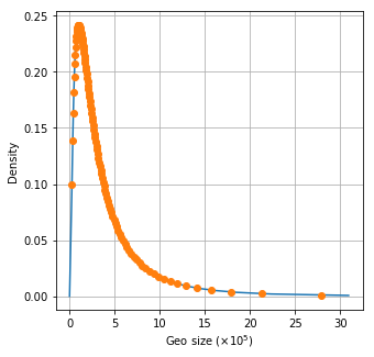
Figure 5.1. Geo sizes (circles) displayed on the lognormal density curve.

We simulate $N=100$ geos for $6$ weeks of pretest data. Figure 5.1 shows the geo sizes $\{g_{i},i=1,\cdots,N\}$ on the lognormal density curve. Figure 5.2 provides a sample of response time series data for a few geos.

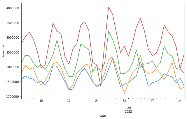
Figure 5.2. Daily time series of the response metric for a few sample geos.

5.2. Result

Consider designing a hold-back experiment with the budget $B=10^{6}$. Suppose the test period is planned to be 2 weeks long and to start soon after the design. The pretest data is split into two time periods: the most recent 4 weeks of data is used for pairing ($\mathcal{T}_{p}$), and the first 2 weeks for evaluation ($\mathcal{T}_{e}$). The purpose of using the latest data for pairing is to best maintain the pairing quality from the pairing period to the test period. By applying the design procedure as described in Section 4, for each $n\in\{10,\cdots,50\}$, the corresponding optimal set of $n$ geo pairs is generated according to the procedure in Section 4.1, and the RMSE value is obtained by Algorithm 1. Regarding the $L$ criteria, in the calculation of the distance (4.1), $T$ spans one week.

The entire simulation is replicated for $M=5000$ times, that is, we use the above data simulation procedure to generate 5000 pretest data sets and rerun the same design process for each of them. Unless specified, any reported result below is an average value across the 5000 replicates.

Effect of geo trimming

With smaller $n$, more geos need to be excluded from the experiment, then we would expect smaller RMSE as discussed in Section 4.1. In Figure 5.3, the x-axis is the number of geo pairs $n$ and the y-axis on the left is the RMSE evaluated using data during $\mathcal{T}_{e}$. As expected, the result shows that RMSE decreases significantly as $n$ decreases. By reducing the number of pairs from 50 to 45, RMSE is reduced by nearly 50%. The red curve (increasing) shows the ratio of budget to the overall base response for the treatment group during $\mathcal{T}_{e}$, which may be helpful for marketing decisions. For example, if $\theta_{0}=2.56$ and the type-I error and the power are set to 10% and 90% respectively, it is desirable to have $RMSE\leq 1$, for which Figure 5.3 suggests $n<30$. On the other hand, from the marketing point of view, if it is preferable that the budget-to-baseline ratio is no more than, say 2%, then the result suggest $n\geq 24$, and thus the optimal design corresponds to $n=24$ as it minimizes the RMSE and thus maximizes the power.

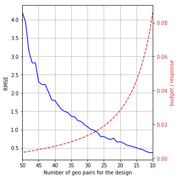
Figure 5.3. RMSE varies with the number of geo pairs, where the red line (increasing) shows the corresponding ratio of budget to baseline response.

Effect of cross validation

To see the effect of cross validation, the RMSE value is also evaluated using the most recent 2 weeks which falls into the pairing period $\mathcal{T}_{p}$. This is shown as the dashed red curve in Figure 5.5, where the solid blue curve corresponds to $\mathcal{T}_{e}$ as reported in Figure 5.3. The result shows that the RMSE value without cross validation is significantly lower than the corresponding RMSE value with cross validation given the same number of geo pairs, which confirms systematic overfitting.

Due to stationarity in the time series data generation, we expect the RMSE evaluation to be unbiased. To verify that, we have also extended the data generation from 6 weeks to 8 weeks and treated the 7th and 8th weeks as the test period to reevaluate the RMSE for each of the 5000 replicates. The average RMSE for each number of geo pairs is reported as the green circles on Figure 5.5. Note that the green circles almost overlap with the solid blue curve, which suggests that the RMSE evaluation with cross validation is indeed unbiased.

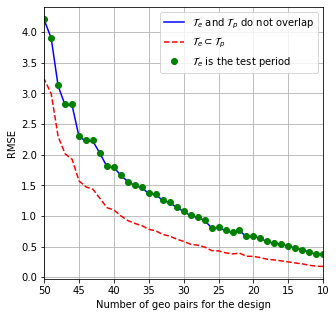
Figure 5.4. Effect of CV.

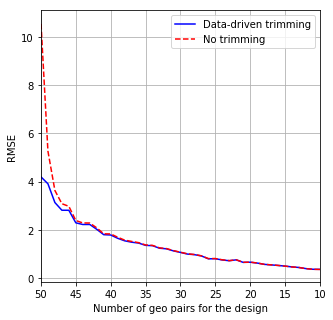
Figure 5.5. Effect of trimming.

Comparison with a design based on permutation test

We also investigate the benefit of using Trimmed Match, over a design based on the standard permutation test, which corresponds to using Trimmed Match with a fixed $\lambda=0$ (see Remark 2). The result is summarized in Figure 5.5, which shows interestingly that the performance is quite comparable except for large $n$. In fact, when $n=50$, Trimmed Match reduces RMSE by a factor larger than 2, which is not surprising though since without trimming, log-normal is indeed much more heavy-tailed than normal. As $n$ gets smaller, larger geos tend to be not matched as they are harder to find comparable geos, and thus the remaining geos tend to be more comparable to each other. Consequently, the response differences tend to be less heavy-tailed, where the ideal trim rate in Trimmed Match is close to 0. This not only validates the robustness of the Trimmed Match estimator but provides some new insights specific to the design process, which has not been studied in Chen and Au (2019).

Choice of the loss function

We also report the performance comparison when the distance (4.1) uses a day instead of a week for $T$, as shown in Figure 5.7. It is interesting to see that the RMSE for $T$ being a week is smaller than that for $T$ being a day when $n$ is large, while the inverse holds when $n$ is small. A heuristic explanation is that for small $n$, the two geos within each pair are quite comparable–more granular comparison (daily instead of weekly here) helps further differentiate geos which are otherwise similar at a coarser granularity.

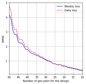
Figure 5.6. Effect of $T$.

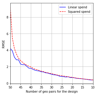
Figure 5.7. Effect of spend.

Sensitivity to the spend proxy

The power calculation of the design is determined by the baseline response and the spend proxy used in the RMSE evaluation. Here we illustrate this by looking at different choices of spend proxy. Note that in the above simulation, the spend proxy (5.1) is proportional to a linear scale of the response, which is often expected. As a comparison, we replicate the above simulation studies, except that the spend proxy in (5.1) is now taken to be proportional to the squared response (which is very extreme) as follows:

(5.2) $$S_{i}(t) \propto\left(R_{i}(t)\right)^{2}\times(1+0.5\times\mathcal{U}_{it}(-1,1)).$$

The RMSE curve as a function of the number of geo pairs for the design is reported by the dotted red line in Figure 5.7, whereas the solid blue line is based on the spend proxy (5.1) as reported earlier. The result shows that when $n$ is close to 50, the squared spend leads to generally higher RMSEs than the linear spend, which can be explained briefly as follows: for the squared spend, too much budget would be spent on the largest geo pair, where the pairing quality is the worst (e.g. the size difference of the largest two geos which makes a pair is more than twice the median geo size, see Figure 5.1), while for the linear spend, the budget is more evenly distributed to geo pairs with better pairing quality, which helps reduce the RMSE. On the other hand, the result also shows that for smaller $n$ (say less than 40), the RMSEs between the linear spend and the squared spend are quite comparable, which suggests that the method is quite robust against potential misspecification of the spend proxy.

6. A case study

In this section we report a real case study, where the experiment was to test a new type of ad. Nielsen’s 210 DMAs were used as the geos, except that a few DMAs were excluded for some other marketing purpose. To design the experiment, more than 1 year of historical revenue (including both offline and online sales) data $R_{g}(t)$ were collected for each geo on a daily basis. To give an idea of the real data, Figure 6.1 shows the weekly time series of $R_{g}(t)\cdot(1+c\cdot U_{g}(t))$ for a few sample geos with both the dates and detailed scales removed, where $\{U_{g}(t):g,t\}$ i.i.d uniformly distributed on $(-1,1)$ and a small constant $c\in(0,1)$ are used to further anonymize the data. The figure shows that unlike the simulated data, the real revenue here is quite non-stationary.

To illustrate the geo heterogeneity, we calculate the aggregated revenue for each geo, sort the geos decreasingly based on the aggregated revenues, and then look at the cumulative revenues of geos, divided by total revenue, which is shown in Figure 6.2, where the x-axis shows the corresponding number of geos in the logarithmic scale. The figure shows that the geo sizes measured by revenues approximately follow a heavy-tailed Pareto distribution, with about 80% of the revenue from 20% of the geos. Some historical ad spend data were also collected to inform the split of the client pre-specified budget.

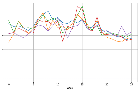
Figure 6.1. Time series of the weekly revenue data for a few geos, where the horizontal dashed line has value 0 while the revenues are jittered and the detailed dates and revenue scales are removed in order to anonymize the experiment.

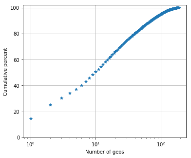
Figure 6.2. Geo-level revenues approximately follow a Pareto distribution.

The experiment was planned for 6 weeks of testing, plus 2 weeks of cooldown to capture any potential lag effects. The evaluation period was taken to be 8 weeks so as to have the same duration as the experiment, and by looking at the seasonality and year-to-year patterns, the 8 weeks were chosen to be the same weeks of the year as the planned experimentation period, but in the previous year. The data after that is used for geo pairing. We investigated two pairing algorithms: optimal pairing as described in Section 4.1 where $T$ is a week, and the rank method which ranks and pairs the geos based on their revenue volumes during the pairing period as described in Remark 1. The RMSE curve as a function of the number of geo pairs is shown in Figure 6.4 for the rank-based pairing (solid blue) and optimal pairing (dashed red) separately. The result tells that, in general, optimal pairing performs significantly better than the simpler rank-based method. Figure 6.4 further plots the ratio of the RMSEs between the two methods for each number of geo pairs and shows that the reduction of RMSE by using optimal pairing compared to the rank-based pairing can be as large as a factor of 3.

The actual design which was employed for the experiment followed the procedure as described in Section 4, except that the pairing algorithm was based on the rank method as optimal pairing was not implemented at that time yet. It used around 60 pairs by applying the budget and other marketing constraints. After the experiment was completed, the point estimate and confidence interval were obtained by the Trimmed Match estimator (see Chen and Au (2019) for the detailed description). It may be interesting to point out that the half width of the $80\%$ two-sided confidence interval is quite comparable to $1.28\times RMSE$, where $RMSE$ was reported from the design phase, despite the irregular temporal dynamics of the revenues.

Figure 6.3. Rank-based pairing vs optimal pairing

Figure 6.4. RMSE ratio between rank-based pairing and optimal pairing

7. Conclusion

We have proposed a robust and cost-effective method for designing randomized paired geo experiments for measuring the incremental return on ad spend. The method integrates optimal pairing, Trimmed Match for estimating iROAS, and cross validation in a novel and systematic manner in order to address both geo heterogeneity and temporal dynamics. The method includes the standard permutation test as a special example when the trim rate in the Trimmed Match estimator is set to 0. By trimming a few geos and constructing an optimal subset of pairs in a data-driven manner, the new method can often reduce the cost by a large factor in real studies. Various open problems exist, such as how to improve the $L$ criterion by taking into account the uncertainty in the data-driven choice of trim rate, how to address random imbalance in a more rigorous manner, and how to adjust the RMSE due to the potential difference between the evaluation period and the test period.

References

- Adwords [2021] Google Adwords. Geo targets. https://developers.google.com/adwords/api/docs/appendix/geotargeting/, 2021. [Online; accessed 21-April-2021].
- Apple [2021] Apple. Data Privacy Day at Apple: Improving transparency and empowering users. https://www.apple.com/newsroom/2021/01/data-privacy-day-at-apple-improving-transparency-and-empowering-users/, 2021. [Online; accessed 7-May-2021].
- Au [2018] Tim Au. A time-based regression matched markets approach for designing geo experiments. 2018. URL https://research.google/pubs/pub48983/.
- Bates et al. [2011] Nancy Bates, Kristin McCue, and Michael Lotti. The paid advertising heavy up experiment. Washington, DC: US Department of Commerce, Census Bureau. Retrieved on August, 18:2014, 2011.
- Bickel and Doksum [2015] Peter J Bickel and Kjell A Doksum. Mathematical statistics: basic ideas and selected topics, volumes I. CRC Press, 2015.
- Blake et al. [2015] Thomas Blake, Chris Nosko, and Steven Tadelis. Consumer heterogeneity and paid search effectiveness: A large-scale field experiment. Econometrica, 83(1):155–174, 2015.
- Box et al. [2005] George EP Box, Stuart Hunter, and William H Hunter. Statistics for experimenters: Design, Innovation, and Discovery, 2nd Edition. Wiley-Interscience, 2005.
- Brodersen et al. [2015] Kay H Brodersen, Fabian Gallusser, Jim Koehler, Nicolas Remy, Steven L Scott, et al. Inferring causal impact using bayesian structural time-series models. Annals of Applied Statistics, 9(1):247–274, 2015.
- Chen and Au [2019] Aiyou Chen and Timothy C Au. Robust causal inference for incremental return on ad spend with randomized paired geo experiments. 2019. URL https://research.google/pubs/pub48448/.
- Chen et al. [2018] Aiyou Chen, David Chan, Mike Perry, Yuxue Jin, Yunting Sun, Yueqing Wang, and Jim Koehler. Bias correction for paid search in media mix modeling. 2018. URL https://research.google/pubs/pub46861/.
- Chen et al. [2020] Aiyou Chen, Marco Longfils, and Christoph Best. The Python library for Trimmed Match and Trimmed Match Design. https://github.com/google/trimmed_match, 2020. [Online; accessed 21-April-2021].
- Coey and Bailey [2016] Dominic Coey and Michael Bailey. People and cookies: Imperfect treatment assignment in online experiments. In Proceedings of the 25th International Conference on World Wide Web, pages 1103–1111, 2016.
- Edmonds [1965] Jack Edmonds. Maximum matching and a polyhedron with 0, 1-vertices. Journal of research of the National Bureau of Standards B, 69(125-130):55–56, 1965.
- GDPR [2021] GDPR. General Data Protection Regulation. https://gdpr.eu/tag/gdpr/, 2021. [Online; accessed 7-May-2021].
- Google [2021] Google. Charting a course towards a more privacy-first web. https://blog.google/products/ads-commerce/a-more-privacy-first-web//, 2021. [Online; accessed 7-May-2021].
- Gordon et al. [2019] Brett R Gordon, Florian Zettelmeyer, Neha Bhargava, and Dan Chapsky. A comparison of approaches to advertising measurement: Evidence from big field experiments at facebook. Marketing Science, 38(2):193–225, 2019.
- Imbens and Rubin [2015] Guido W Imbens and Donald B Rubin. Causal inference in statistics, social, and biomedical sciences. Cambridge University Press, 2015.
- Johnson et al. [2017] Garrett A Johnson, Randall A Lewis, and Elmar I Nubbemeyer. Ghost ads: Improving the economics of measuring online ad effectiveness. Journal of Marketing Research, 54(6):867–884, 2017.
- Kerman et al. [2017] Jouni Kerman, Peng Wang, and Jon Vaver. Estimating ad effectiveness using geo experiments in a time-based regression framework. 2017. URL https://research.google/pubs/pub45950/.
- Kohavi et al. [2020] Ron Kohavi, Diane Tang, and Ya Xu. Trustworthy online controlled experiments: A practical guide to a/b testing. Cambridge University Press, 2020.
- Kolmogorov [2009] Vladimir Kolmogorov. Blossom v: a new implementation of a minimum cost perfect matching algorithm. Mathematical Programming Computation, 1(1):43–67, 2009.
- Li and Ding [2020] Xinran Li and Peng Ding. Rerandomization and regression adjustment. Journal of the Royal Statistical Society: Series B, 82(1):241–268, 2020.
- Lu et al. [2001] Bo Lu, Elaine Zanutto, Robert Hornik, and Paul R Rosenbaum. Matching with doses in an observational study of a media campaign against drug abuse. Journal of the American Statistical Association, 96(456):1245–1253, 2001.
- Morgan et al. [2012] Kari Lock Morgan, Donald B Rubin, et al. Rerandomization to improve covariate balance in experiments. The Annals of Statistics, 40(2):1263–1282, 2012.
- Nair et al. [1992] Vijayan N Nair, Bovas Abraham, Jock MacKay, George Box, Raghu N Kacker, Thomas J Lorenzen, James M Lucas, Raymond H Myers, G Geoffrey Vining, John A Nelder, et al. Taguchi’s parameter design: a panel discussion. Technometrics, 34(2):127–161, 1992.
- Papadimitriou and Steiglitz [1998] Christos H Papadimitriou and Kenneth Steiglitz. Combinatorial optimization: algorithms and complexity. Courier Corporation, 1998.
- Rolnick et al. [2019] David Rolnick, Kevin Aydin, Jean Pouget-Abadie, Shahab Kamali, Vahab Mirrokni, and Amir Najmi. Randomized experimental design via geographic clustering. In Proceedings of the 25th ACM SIGKDD International Conference on Knowledge Discovery & Data Mining, pages 2745–2753, 2019.
- Rosenbaum [2020] Paul R Rosenbaum. Design of observational studies, 2nd Edition, volume 10. Springer, 2020.
- Sapp et al. [2017] Stephanie Sapp, Jon Vaver, Jon Schuringa, and Steven Dropsho. Near impressions for observational causal ad impact. 2017. URL https://research.google/pubs/pub46418/.
- Stuart [2010] Elizabeth A Stuart. Matching methods for causal inference: A review and a look forward. Statistical science, 25(1):1, 2010.
- Tibshirani [1996] Robert Tibshirani. Regression shrinkage and selection via the lasso. Journal of the Royal Statistical Society: Series B, 58(1):267–288, 1996.
- Tukey [1993] John W Tukey. Tightening the clinical trial. Controlled clinical trials, 14(4):266–285, 1993.
- Varian [2016] Hal R Varian. Causal inference in economics and marketing. Proceedings of the National Academy of Sciences, 113(27):7310–7315, 2016.
- Vaver and Koehler [2011] Jon Vaver and Jim Koehler. Measuring ad effectiveness using geo experiments. 2011. URL https://research.google.com/pubs/pub38355.html.
- Wu and Hamada [2020] CF Jeff Wu and Michael S Hamada. Experiments: Planning, Analysis, and Optimization. John Wiley & Sons, 2020.
- Ye et al. [2016] Quinn Ye, Saarthak Malik, Ji Chen, and Haijun Zhu. The seasonality of paid search effectiveness from a long running field test. In Proceedings of the 2016 ACM Conference on Economics and Computation, pages 515–530, 2016.
- Yen et al. [2012] Ting-Fang Yen, Yinglian Xie, Fang Yu, Roger Peng Yu, and Martin Abadi. Host fingerprinting and tracking on the web: Privacy and security implications. In NDSS, volume 62, page 66, 2012.