Subgraph Games in the Semi-Random Graph Process and Its Generalization to Hypergraphs

Abstract.

The semi-random graph process is a single-player game that begins with an empty graph on $n$ vertices. In each round, a vertex $u$ is presented to the player independently and uniformly at random. The player then adaptively selects a vertex $v$ and adds the edge $uv$ to the graph. For a fixed monotone graph property, the objective of the player is to force the graph to satisfy this property with high probability in as few rounds as possible.

We focus on the problem of constructing a subgraph isomorphic to an arbitrary, fixed graph $G$. Let $\omega=\omega(n)$ be any function tending to infinity as $n\to\infty$. In [2] it was proved that asymptotically almost surely one can construct $G$ in less than $n^{(d-1)/d}\omega$ rounds where $d\geq 2$ is the degeneracy of $G$. It was also proved that the result is sharp for $G=K_{d+1}$, that is, asymptotically almost surely it takes at least $n^{(d-1)/d}/\omega$ rounds to create $K_{d+1}$. Moreover, the authors of [2] conjectured that their general upper bound is sharp for all graphs $G$. We prove this conjecture here.

We also consider a natural generalization of the process to $s$-uniform hypergraphs, the semi-random hypergraph process in which $r\geq 1$ vertices are presented at random, and the player then selects $s-r\geq 1$ vertices to form an edge of size $s$. Our results for graphs easily generalize to hypergraphs when $r=1$; the threshold for constructing a fixed $s$-uniform hypergraph $G$ is, again, determined by the degeneracy of $G$. However, new challenges are mounting when $r\geq 2$; thresholds are not even known for complete hypergraphs. We provide bounds for this family and determine thresholds for some sparser hypergraphs.

1. Introduction

In this paper, we consider the semi-random process suggested by Peleg Michaeli and studied recently in [2, 1, 4, 5] that can be viewed as a “one player game”.

1.1. Definitions and background

The process starts from $H_{0}$, the empty graph on the vertex set $[n]:=\{1,2,\ldots,n\}$ where $n\geq 1$. In each step $t\geq 1$, a vertex $u_{t}$ is chosen uniformly at random from $[n]$. Then, the player (who is aware of graph $H_{t-1}$ and vertex $u_{t}$) must select a vertex $v_{t}$ and add the edge $u_{t}v_{t}$ to $H_{t-1}$ to form $H_{t}$. The goal of the player is to build a (multi)graph satisfying a given property $\mathcal{P}$ as quickly as possible. It is convenient to think of $u_{t}$ as receiving a square, and $v_{t}$ as receiving a circle, so every edge in $H_{t}$ joins a square with a circle. Equivalently, we may view $H_{t}$ as a directed graph where arcs go from $u_{i}$ to $v_{i}$, $i=1,\dots,t$.

A strategy $\mathcal{S}$ is defined by specifying, for each $n\geq 1$, a sequence of functions $(f_{t})_{t=1}^{\infty}$, where for each $t\in{\mathbb{N}}$, $f_{t}(u_{1},v_{1},\ldots,u_{t-1},v_{t-1},u_{t})$ is a distribution over $[n]$ which depends on the vertex $u_{t}$, and the history of the process up until step $t-1$. Then, $v_{t}$ is chosen according to this distribution. If $f_{t}$ is an atomic distribution, that is non-random, then $v_{t}$ is fully determined by $u_{1},v_{1},\ldots,u_{t-1},v_{t-1},u_{t}$. We denote by $(H_{i}^{\mathcal{S}}(n))_{i=0}^{t}$ the sequence of random (multi)graphs obtained by following the strategy $\mathcal{S}$ for $t$ rounds; we shorten $H_{t}^{\mathcal{S}}(n)$ to $H_{t}$ or $H_{t}(n)$ when clear. To make the process well-defined, we allow parallel edges (for example, if some vertex receives $n$ squares, a parallel edge is necessary). We will also allow loops, as this will be useful in some proofs.

The semi-random process was studied in the context of perfect matchings and Hamilton cycles in [2, 4, 5]. In all of these results, the length of the process leading to establishing a given property is of order $\Theta(n)$, though the multiplicative constant was not determined precisely. However, more closely related to the topic of this paper is the property of containing a given graph $H$ as a spanning subgraph, which we will discuss in more detail.

We say that an event holds asymptotically almost surely (a.a.s.) if it holds with probability tending to one as $n\to\infty$. As was reported in [1], Noga Alon asked whether for any graph $G$ with $\Delta(G)\leq\Delta$ and at most $n$ vertices, one can construct a copy of $G$ in $H_{t}$ a.a.s. for $t=O(n)$. This question was answered positively in a strong sense in [1], where it was shown that such a $G$ can be constructed a.a.s. in $(3\Delta/2+o(\Delta))n$ rounds. They also proved that if $\Delta=\omega(\log(n))$, then this upper bound improves to $(\Delta/2+o(\Delta))n$ rounds. Note that this result applies to fixed subgraphs too, but this bound is far too weak. Indeed, we will show that the property of containing a fixed subgraph has a threshold of order $o(n)$. Consequently, we will be interested in finding the correct exponent of $n$ rather than multiplicative constants.

The semi-random process may be extended or generalized in various ways. For example, in [6] the authors consider a no-replacement variant of the process in which squares follow a permutation of vertices selected uniformly at random. Once each vertex is covered with a square, another random permutation is drawn, and the process continues.

In this paper, we propose a natural generalization of the semi-random process to hypergraphs. Fix $r\geq 1$ to be the number of randomly selected vertices per step, and $s\geq r$ to be the uniformity of the hypergraph. The process starts from $H^{(r,s)}_{0}$, the empty hypergraph on the vertex set $[n]$, where $n\geq 1$. In each step $t\geq 1$, a set $U_{t}$ of $r$ vertices is chosen uniformly at random from $[n]$. Then, the player replies by selecting a set of $s-r$ vertices $V_{t}$ and the edge $U_{t}\cup V_{t}$ is added to $H^{(r,s)}_{t-1}$ to form $H^{(r,s)}_{t}$. As was the case with graphs, in order for the process to be well defined and to simplify some of our proofs, we will allow parallel edges and overlapping pairs $(U_{t},V_{t})$, which are a natural generalization of loops in the case of graphs. (Of course, for most hypergraph properties, creating loops or parallel edges is not part of an optimal strategy.)

Note that the resulting hypergraph is $s$-uniform, or shortly an $s$-graph, provided that edges are treated as multisets. If $r=1$ and $s=2$, then this is the semi-random graph process described above. On the other hand, if $r=s$ (that is, the player chooses $V_{t}=\emptyset$ for all $t$), then $H_{t}^{(r,r)}$ is just a uniform random $r$-graph process with $t$ edges selected with repetitions.

As before, the goal of the player is to build an $s$-graph $H_{t}^{(r,s)}$ satisfying a given property $\mathcal{P}$ as quickly as possible, and we focus on the property $\mathcal{P}_{G}$ of possessing a sub-$s$-graph isomorphic to an arbitrary, fixed $s$-graph $G$.

1.2. Main Results

Suppose $\mathcal{P}$ is a monotonically increasing property of $s$-uniform hypergraphs. Given a strategy $\mathcal{S}$, integer $1\leq r\leq s-1$, and a constant $0<q<1$, let $\tau^{(r)}_{\mathcal{P}}(\mathcal{S},q,n)$ be the minimum $t\geq 0$ for which $\mathbb{P}[H^{(r,s)}_{t}\in\mathcal{P}]\geq q$, where $\tau^{(r)}_{\mathcal{P}}(\mathcal{S},q,n):=\infty$ if no such $t$ exists. Define

$$\tau^{(r)}_{\mathcal{P}}(q,n)=\inf_{\mathcal{S}}\tau^{(r)}_{\mathcal{P}}(\mathcal{S},q,n),$$ (1.1)

where the infimum is over all strategies on $[n]$. Observe that for each $n\geq 1$, if $0\leq q_{1}\leq q_{2}\leq 1$, then $\tau^{(r)}_{\mathcal{P}}(q_{1},n)\leq\tau^{(r)}_{\mathcal{P}}(q_{2},n)$, as $\mathcal{P}$ is monotonically increasing. Thus, the function $q\mapsto\limsup_{n\to\infty}\ln(\tau^{(r)}_{\mathcal{P}}(q,n))$ is non-decreasing, and so the limit

$$\tau^{(r)}_{\mathcal{P}}:=\lim_{q\to 1^{-}}\limsup_{n\to\infty}\frac{\ln(\tau^{(r)}_{\mathcal{P}}(q,n))}{\ln n}$$

is guaranteed to exist (with the convention that it can be equal to $\infty$). The goal is typically to compute upper and lower bounds on $\tau^{(r)}_{\mathcal{P}}$ for various properties $\mathcal{P}$. In this paper, we focus on the problem of constructing a sub-hypergraph isomorphic to an arbitrary, fixed hypergraph $G$. Let $\mathcal{P}_{G}$ be the property that $G\subseteq H^{(r,s)}_{t}$.

It turns out that for $r=1$, that is, when just a single vertex is selected randomly at every step, the threshold $\tau_{\mathcal{P}_{G}}$ can be determined in terms of the degeneracy of $G$ (we suppress the dependence on $r$ when $r=1$). For a given $d\in{\mathbb{N}}$, a hypergraph $G$ is $d$-degenerate if every sub-hypergraph $G^{\prime}\subseteq G$ has minimum degree $\delta(G^{\prime})\leq d$. The degeneracy of $G$ is the smallest value of $d$ for which $G$ is $d$-degenerate. The $d$-core of a hypergraph $G$ is the maximal induced subgraph $G^{\prime}\subseteq G$ with minimum degree $\delta(G^{\prime})\geq d$. (Note that the $d$-core is well defined, though it may be empty. Indeed, if $S\subseteq V(G)$ and $T\subseteq V(G)$ induce sub-hypergraphs with minimum degree at least $d$, then the same is true for $S\cup T$.) If $G$ has degeneracy $d$ then it has a non-empty $d$-core. Indeed, by definition, $G$ is not $(d-1)$-degenerate and so it has a sub-hypergraph $G^{\prime}$ with $\delta(G^{\prime})\geq d$. We immediately get that if $G$ has degeneracy $d$, then there exists a permutation of the vertices of $G$, $(v_{1},v_{2},\ldots,v_{k})$, such that for each $\ell\in[k]$ vertex $v_{\ell}$ has degree at most $d$ in the sub-hypergraph induced by the set $\{v_{1},v_{2},\ldots,v_{\ell}\}$.

For graphs, this implies a useful reformulation of degeneracy: a graph $G$ is $d$-degenerate if and only if the edges of $G$ can be oriented to form a directed acyclic graph $D$ with maximum out-degree at most $d$. In other words, there exists a permutation of the vertices of $G$, $(v_{1},v_{2},\ldots,v_{k})$, such that for every directed edge $(v_{i},v_{j})\in D$ we have $i>j$ (and the out-degrees are at most $d$).

It was proved in [2] that for any graph $G$ of degeneracy $d\in{\mathbb{N}}$, $\tau_{\mathcal{P}_{G}}\leq(d-1)/d$.

Theorem 1.1 ([2]).

Let $G$ be a fixed graph of degeneracy $d\in{\mathbb{N}}$. Then, there exists a strategy $\mathcal{S}$ such that

$$\lim_{n\to\infty}\mathbb{P}[H_{t}\in\mathcal{P}_{G}]=1,$$

where $t=n^{(d-1)/d}\omega$ and $\omega=\omega(n)$ is any function tending to infinity as $n\to\infty$.

For completeness and as a warm-up, we re-prove that result in Section 2.2.

Note that for $d=1$, that is, when $G$ is a forest, Theorem 1.1 implies immediately that $\tau^{(r)}_{\mathcal{P}_{G}}=0$. For $d\geq 2$, it was proved in [2] that $\tau_{\mathcal{P}_{G}}=(d-1)/d$ when $G=K_{d+1}$, the complete graph on $d+1$ vertices, and conjectured that the equality holds for all graphs of degeneracy $d$. As our main result, we prove this conjecture here.

Theorem 1.2.

Let $G$ be a fixed graph of degeneracy $d\geq 2$. Then, for any strategy $\mathcal{S}$

$$\lim_{n\to\infty}\mathbb{P}[H_{t}\in\mathcal{P}_{G}]=0,$$

where $t=n^{(d-1)/d}/\omega$ and $\omega=\omega(n)$ is any function tending to infinity as $n\to\infty$.

Combining Theorems 1.1 and 1.2 we get the following corollary.

Corollary 1.3.

Let $G$ be a fixed graph of degeneracy $d\in{\mathbb{N}}$. Then, $\tau_{\mathcal{P}_{G}}=(d-1)/d$.

In Section 3 we show that for uniform hypergraphs, the case $r=1$ resembles the graph case and the degeneracy of an $s$-uniform hypergraph $G$ is still the only parameter that affects the threshold for the property $G\subseteq H_{t}^{(1,s)}$. In particular, we have the following theorems that are counterparts of Theorem 1.1 and Theorem 1.2.

Theorem 1.4.

Let $r=1$, $s\geq 2$, and let $G$ be a fixed $s$-uniform hypergraph of degeneracy $d\in{\mathbb{N}}$. Then, there exists a strategy $\mathcal{S}$ such that

$$\lim_{n\to\infty}\mathbb{P}[H_{t}^{(r,s)}\in\mathcal{P}_{G}]=1,$$

where $t=n^{(d-1)/d}\omega$ and $\omega=\omega(n)$ is any function tending to infinity as $n\to\infty$.

Theorem 1.5.

Let $r=1$, $s\geq 2$, and let $G$ be a fixed $s$-uniform hypergraph of degeneracy $d\geq 2$. Then, for any strategy $\mathcal{S}$ we have that

$$\lim_{n\to\infty}\mathbb{P}[H_{t}^{(r,s)}\in\mathcal{P}_{G}]=0,$$

where $t=n^{(d-1)/d}/\omega$ and $\omega=\omega(n)$ is any function tending to infinity as $n\to\infty$.

As a result, combining Theorems 1.4 and 1.5, we get the following corollary.

Corollary 1.6.

Let $r=1$ and let $G$ be a fixed uniform hypergraph of degeneracy $d\in{\mathbb{N}}$. Then, $\tau_{\mathcal{P}_{G}}=(d-1)/d$.

The proofs of these results follow the same approach as in the graph case.

Our understanding of the semi-hypergraph process with $r\geq 2$ is far from being complete. For the property $\mathcal{P}_{G}$, we can only prove a general lower bound and show it is optimal for particular classes of hypergraphs.

Theorem 1.7.

Let $k\geq s\geq r\geq 2$, and let $G$ be an $s$-uniform hypergraph with $k$ vertices and $m$ edges. Then, for any strategy $\mathcal{S}$ we have that

$$\lim_{n\to\infty}\mathbb{P}[H^{(r,s)}_{t}\in\mathcal{P}_{G}]=0,$$

where $t=n^{r-(k-s+r)/m}/\omega$ and $\omega=\omega(n)$ is any function tending to infinity as $n\to\infty$. As a result, $\tau^{(r)}_{\mathcal{P}_{G}}\geq r-(k-s+r)/m$.

Of course, it might happen that the main “bottleneck” is not the original hypergraph $G$ as a whole, but one of its sub-hypergraphs $G^{\prime}\subseteq G$. Trivially, creating $G$ requires creating $G^{\prime}$ in the first place, so we immediately obtain the following corollary.

Corollary 1.8.

Let $k\geq s\geq r\geq 2$, and let $G$ be an $s$-uniform hypergraph. Define

$$\mu_{G}^{(r,s)}=\max_{G^{\prime}\subseteq G,\ |V(G^{\prime})|\geq s}\frac{|E(G^{\prime})|}{|V(G^{\prime})|-s+r}.$$

Then,

$$\tau^{(r)}_{\mathcal{P}_{G}}\geq r-\frac{1}{\mu_{G}^{(r,s)}}.$$

Note that, by considering a single edge as $G^{\prime}$, we always have $\mu_{G}^{(r,s)}\geq 1/r$, and so the lower bound in Corollary 1.8 cannot be negative. However, for most hypergraphs $G$ we have $\mu_{G}^{(r,s)}>1/r$, giving us a nontrivial lower bound for $\tau^{(r)}_{\mathcal{P}_{G}}$. Note also that in the special case when $r=s$, we are looking at the random $s$-graph (with repeated edges) and the bound in Corollary 1.8 corresponds to the threshold for appearance of a copy of a given $s$-graph $G$ (see [7, Chapter 3] for the case $r=s=2$ or [3] for non-uniform hypergraphs (both results do not allow repetitions)).

For integers $1\leq c\leq s\leq k$, a $k$-vertex $s$-graph is called a full $c$-star if its edge set consists of all $\binom{k-c}{s-c}$ $s$-tuples containing a fixed vertex set $C$ of size $|C|=c$ – the center of the star. For $c=1$, this is the ordinary $s$-uniform full star. An $(s,c)$-starplus of excess $\ell$ is defined as any $s$-graph obtained from a full $c$-star by arbitrarily adding to it $\ell$ edges. For $c>1$, the additional edges may intersect the center $C$.

For starpluses $G$ which are not too dense, we have an upper bound on $\tau^{r}_{\mathcal{P}_{G}}$, where $r=s-c$, which matches the lower bound established in Theorem 1.7.

Theorem 1.9.

Let $r\geq 2$ and $s>r$, and let $G$ be an $(s,s-r)$-starplus on $k$ vertices with excess

$$\ell\leq\frac{r\binom{k-s+r}{r}-(k-s+r)}{k-s}.$$ (1.2)

Then, there exists a strategy $\mathcal{S}$ such that

$$\lim_{n\to\infty}\mathbb{P}[H_{t}^{(r,s)}\in\mathcal{P}_{G}]=1,$$

where

$$t=n^{r-\frac{k-s+r}{\binom{k-s+r}{r}+\ell}}\omega$$

and $\omega=\omega(n)$ is any function tending to infinity as $n\to\infty$. Thus, in view of Theorem 1.7,

$$\tau^{(r)}_{\mathcal{P}_{G}}=r-\frac{k-s+r}{\binom{k-s+r}{r}+\ell}.$$

It follows from Theorem 1.9 that, in view of Corollary 1.8 any $(s,s-r)$-starplus $G$ satisfying (1.2) is balanced in the sense that $\mu_{G}^{(r,s)}=\frac{|E(G)|}{|V(G)|-s+r}$, a fact that can be proved separately by quite tedious calculations (see the Appendix).

The family of $s$-graphs to which Theorem 1.9 applies includes even some small cliques. Indeed, since cliques cane b viewed as $(s,s-r)$-starpluses with excess $\ell=\binom{k}{s}-\binom{k-s+r}{r}$, assumption (1.2) is equivalent to

$$\binom{k}{s}\leq\frac{k-s+r}{k-s}\left(\binom{k-s+r}{r}-1\right).$$

Thus, in particular, Theorem 1.9 covers cliques $K_{s+1}^{(s)}$, whenever $s\leq r^{2}+r-1$ and cliques $K_{s+2}^{(s)}$, whenever $(s+2)(s+1)\leq\tfrac{1}{2}r(r+2)(r+3)$. When $r=s-1$, assumption (1.2) for cliques becomes

$$\binom{k-1}{s}\leq\frac{(s-1)\binom{k-1}{s-1}-(k-1)}{k-s}$$

which holds whenever $k\leq 2s-1$. So, in addition, Theorem 1.9 covers cliques $K_{7}^{(4)}$ (for $r=3$), $K_{8}^{(5)}$, $K_{9}^{(5)}$ (for $r=4$), and so on. The smallest open case among cliques is thus $G=K_{6}^{(3)}$ and $r=2$ (see the end of this subsection for an upper bound on $\tau^{(2)}_{\mathcal{P}_{G}}$).

An interesting non-complete instance of Theorem 1.9 is when the surplus edges of $G$ form a tight $s$-cycle on the vertex set $V(G)\setminus C$. A tight cycle $C_{q}^{(s)}$ is defined as an $s$-graph with $q$ vertices and $q$ edges, whose vertices can be ordered cyclically so that the edges are formed by the consecutive $s$-element segments in this ordering. (E.g., triples $123,234,345,456,567,671,712$ form a copy of $C_{7}^{(3)}$.) As $\ell=q=k-s+r$, we have that for all $2\leq r<s$ such $(s,s-r)$-starpluses $G$ satisfy assumption (1.2) and thus $\tau^{(r)}_{\mathcal{P}_{G}}=r-\frac{q}{\binom{q}{r}+q}.$

Another non-complete example of a starplus covered by Theorem 1.9 is presented in Figure 2 in Section 4. It is a full $3$-uniform 1-star on 8 vertices topped with a Fano plane. In fact, as for $r=2$ and $s=3$ the upper bound on excess in (1.2) is $k-1$, it is the densest 3-uniform starplus on $k=8$ vertices to which Theorem 1.9 applies.

The ideas used in the proof of Theorem 1.9 can be extended to families of $s$-graphs violating assumption (1.2), but the obtained bounds may not always match the lower bound in Theorem 1.7. (See Subsection 4.3 for more discussion on this.) On the other hand, Theorem 1.9 can be used as a black box to derive a generic upper bound on $\tau^{(r)}_{\mathcal{P}_{G}}$ in terms of just the maximum degree and the number of edges of the $s$-graph $G$. For $1\leq d\leq s$, let $\Delta_{d}(G)$ denote the maximum degree of a $d$-set of vertices of $G$, i.e., the maximum number of edges that contain any given subset $D\subset V(G)$, $|D|=d$.

Corollary 1.10.

Let $s>r\geq 2$ and let $G$ be an arbitrary $s$-graph. Further, let $k$ be the smallest integer for which (1.2) holds with $\ell:=e(G)-\Delta_{s-r}(G)$. Then

$$\tau^{(r)}_{\mathcal{P}_{G}}\leq r-\frac{k-s+r}{\binom{k-s+r}{r}+\ell}.$$

Proof.

Let $C\subset V(G)$, $|C|=s-r$, be a subset which achieves the maximum in the definition of $\Delta_{s-r}(G)$. Further, let $G^{\prime}$ be a subgraph of $G$ obtained by deleting all edges containing $C$. Apply Theorem 1.9 to an $(s,s-r)$-starplus $\bar{G}$ on $k$ vertices and with the $\ell$ surplus edges forming a copy of $G^{\prime}$. Clearly, $\bar{G}\supset G$ and the statement follows by monotonicity. ∎

This bound is generally very weak, but its strength lies in its universality. In particular, it implies that $\tau^{(r)}_{\mathcal{P}_{G}}<r$ for all $s$-graphs $G$. In some cases, however, it is not so bad. Consider, for instance, the clique $G:=K_{6}^{(3)}$ and $r=2$. We have $e(G)=20$ and $\Delta_{1}(G)=10$. So, we may set $\ell:=20-10-10$ and, remembering that the R-H-S of (1.2) in this case is just $k-1$, apply Corollary 1.10 with $k=11$, obtaining the bound $\tau^{(2)}_{\mathcal{P}_{G}}\leq 2-\tfrac{2}{11}$, not so far from $2-\tfrac{1}{4}$, the lower bound. In Subsection 4.3, with quite an effort, we improve this upper bound to only $\tau^{(2)}_{\mathcal{P}_{F}}\leq 2-\tfrac{1}{5}$.

1.3. Organization

In the next section we prove Theorems 1.1 and 1.2, while in Section 3 – Theorems 1.4 and 1.5. Section 4 contains the proofs of Theorems 1.7 and 1.9, as well as some further results on hypergraphs, $r\geq 2$. Finally, the last section presents a number of open problems.

2. Proofs for graphs

2.1. Useful Lemma

Let us first state the following simple but useful lemma. Proofs of Theorems 1.1 and 1.2, as well as (since the lemma does not depend on $s$) of Theorems 1.4 and 1.5, will rely on it.

Lemma 2.1.

Let $t=o(n)$ and let $\omega=\omega(n)$ be any function tending to infinity as $n\to\infty$. Let $x\in{\mathbb{N}}$ and let $X_{t}^{(x)}$ be the number of vertices in $H_{t}$ with precisely $x$ squares on them, that is, the number of vertices in $H_{t}$ with out-degree $x$. Then the following holds:

• $\mathbb{E}X_{t}^{(x)}=(1-o(1))\frac{t^{x}}{x!n^{x-1}}$.

• If $t=n^{(x-1)/x}/\omega$, then a.a.s. $X_{t}^{(x)}=0$.

• If $t=n^{(x-1)/x}\omega$, then for any $y\in{\mathbb{N}}$ a.a.s. $X_{t}^{(x)}\geq y$.

Proof.

Let $Y_{t}(i)$, $i=1,\dots,n$, be the number of square on vertex $i$ in $H_{t}$. It follows from our random model that each $Y_{t}(i)$ is a random variable with the binomial distribution $Bin(t,1/n)$. Note, however, that the $Y_{t}(i)$’s are not independent. The same observation applies to the indicator random variables $I_{t}(i)^{(x)}$, where for each $i=1,\dots n$, $I_{t}(i)^{(x)}=1$ if $Y_{t}(i)=x)$ and 0 otherwise. Thus

$$X_{t}^{(x)}=\sum_{i=1}^{n}I_{t}(i)^{(x)},$$

and, since $t=o(n)$ and $x$ is a constant, we immediately get that

$$\mathbb{E}X_{t}^{(x)} = n\binom{t}{x}\left(\frac{1}{n}\right)^{x}\left(1-\frac{1}{n}\right)^{t-x}$$

$$= (1-o(1))\frac{nt^{x}}{x!n^{x}}\exp\left(-\frac{t-x}{n}+O(t/n^{2})\right)$$

$$= (1-o(1))\frac{t^{x}}{x!n^{x-1}}.$$

If $t=n^{(x-1)/x}/\omega$, then $\mathbb{E}X_{t}^{(x)}=o(1)$ and so a.a.s. $X_{t}^{(x)}=0$ by the first moment method. On the other hand, if $t=n^{(x-1)/x}\omega$, then $\mathbb{E}X_{t}^{(x)}\sim\omega^{x}/x!\to\infty$ as $n\to\infty$. Set $X:=X_{t}^{(x)}$ for convenience. To turn the above estimate of expectation $\mathbb{E}X$ into the desired lower bound on $X$ itself, we are going to apply the second moment method, or Chebyshev’s inequality, with the variance expressed in terms of the second factorial moment (this form fits well the cases when all summands constituting $X$ are pairwise dependent):

$$\mathbb{P}\left(|X-\mathbb{E}X|>\frac{1}{2}\mathbb{E}X\right)\leq\frac{4\mathrm{Var}(X)}{(\mathbb{E}X)^{2}}=4\left(\frac{\mathbb{E}(X(X-1))}{(\mathbb{E}X)^{2}}+\frac{1}{\mathbb{E}X}-1\right).$$ (2.1)

Since $\mathbb{E}X\to\infty$ as $n\to\infty$, it suffices to show that $\mathbb{E}(X(X-1))\sim(\mathbb{E}X)^{2}$. By symmetry,

$$\mathbb{E}(X(X-1))=n(n-1)\mathbb{P}(I_{t}(1)^{(x)}=I_{t}(2)^{(x)}=1),$$

while

$$\mathbb{P}(I_{t}(1)^{(x)}=I_{t}(2)^{(x)}=1)=\binom{t}{x}\binom{t-x}{x}\left(\frac{1}{n}\right)^{2x}\left(1-\frac{2}{n}\right)^{t-2x}\sim\frac{t^{2x}}{x!^{2}n^{2x}},$$

and, thus, indeed, $\mathbb{E}(X(X-1))\sim(\mathbb{E}X)^{2}$. Consequently, a.a.s. $X_{t}^{(x)}\geq\omega^{x}/(3x!)$ and, in particular, $X_{t}^{(x)}\geq y$, regardless of the value of $y\in{\mathbb{N}}$. ∎

2.2. Upper Bound

In this section we will re-prove Theorem 1.1. We do it for completeness as well as to highlight challenges in proving the lower bound.

Proof of Theorem 1.1.

Let $G$ be a graph on $k$ vertices $V(G)=\{v_{1},v_{2},\ldots,v_{k}\}$ of degeneracy $d\in{\mathbb{N}}$. As such, we may assume that for each $\ell\in[k]$, vertex $v_{\ell}$ has at most $d$ neighbours among $\{v_{1},v_{2},\ldots,v_{i-1}\}$. We orient edges of $G$ such that all edges are from $v_{i}$ to $v_{j}$ for some $j<i$. As a result, the maximum out-degree is equal to $d$.

The player can create the oriented graph $G$ in $t=n^{(d-1)/d}\omega$ rounds by using the following simple strategy. The process is divided into $k$ phases labelled with $\ell\in[k]$, each consisting of $t/k$ rounds. At the beginning of phase $\ell$, we assume that a copy of the induced subgraph $G[\{v_{1},v_{2},\ldots,v_{\ell-1}\}]$ has been already created in $H_{(\ell-1)t/k}$. (Note that the property is trivially satisfied at the beginning of phase $\ell=1$.) Let us fix one such copy and let $u_{i}$ be the image of $v_{i}$, $i=1,\dots,\ell-1$ in that copy.

Let $N_{\ell}\subseteq\{v_{1},v_{2},\ldots,v_{\ell-1}\}$ be the neighbours of $v_{\ell}$ in $G$ that come earlier in the vertex ordering. By construction, $h:=|N_{\ell}|\leq d$. Let $w_{1},\dots,w_{h}$ be the images of the vertices of $N_{\ell}$ in the fixed copy of $G[\{v_{1},v_{2},\ldots,v_{\ell-1}\}]$ in $H_{(\ell-1)t/k}$.

The goal of the player (in this phase) is to create an image $u_{\ell}$ of vertex $v_{\ell}$ that is adjacent to $w_{1},\dots,w_{h}$. In order to achieve this, when some vertex receives its $i$th square during this phase, $1\leq i\leq h$, the player simply connects this vertex with $w_{i}$. It follows from Lemma 2.1(c) with $x=d$ and $y=k$ that a.a.s. at least $k$ vertices receive $d$ squares during this phase, and since a.a.s. these $k$ vertices do not include vertices in $u_{1},\dots,u_{\ell-1}$, the fixed copy of $G[\{v_{1},v_{2},\ldots,v_{\ell-1}\}]$ can be extended to a copy of $G[\{v_{1},v_{2},\ldots,v_{\ell-1},v_{\ell}\}]$. Since the number of phases is $k=O(1)$, a.a.s. a copy of $G$ is created in $k$ phases, and the proof is finished. ∎

2.3. Lower Bound

In this section, we prove the main result of this paper, Theorem 1.2. The theorem holds even when the graph $G$ contains loops or parallel edges. Indeed, for the purposes of the proof we will need this slightly stronger setting.

Let $G$ be a graph on $k$ vertices and $m$ edges that may contain loops and parallel edges. Fix an ordering of the edges $(e_{1},e_{2},\ldots,e_{m})$ of $G$, and fix an orientation of each edge. We will analyze the probability of an oriented copy of $G$ arising in $H_{t}$ where the edges of $G$ are added to $H_{t}$ in this specified order and the edge orientations in $H_{t}$ (from squares to circles) respect the edge orientations of $G$. Since, for a fixed $G$, there is only a finite number of ways to order and orient the edges, we can sum these probabilities to get the desired bound on the occurrence of any copy of $G$ in $H_{t}$. Later on, we will formally prove this simple observation but for now, let us restrict ourselves to a given orientation and a given order of edges, and assume that the goal of the player is to create a copy of $G$ with these additional constraints.

To highlight the main challenge in proving the result, consider a simple example with $G=C_{4}$, the cycle of length 4. If the cycle is oriented such that one of the vertices has out-degree 2, then it follows immediately from Lemma 2.1(c) that a.a.s. one needs at least $\sqrt{n}/\omega$ rounds to accomplish the task, and we are done. However, if the cycle is oriented such that each vertex has out-degree 1, then no non-trivial bound can be deduced from the lemma.

In order to deal with all possible scenarios, for a given orientation and order, we define a weight function on the vertices of the graph $G$. This function is meant to measure how much of the difficulty in creating a copy of $G$ hinges upon a given vertex. We will then show (see Lemma 2.2) that if $G$ is $d$-degenerate, then all vertices of its $d$-core $G^{\prime}$ have weight at least $d$. On the other hand, we will show (see Lemma 2.3) that even if $G^{\prime}$ contains just one vertex of weight at least $d$, then the expected number of copies of $G^{\prime}$ in $H_{t}$ is at most $O(t^{d}/n^{d-1})$, regardless of the strategy of the player. As a result, if $t=o(n^{(d-1)/d})$, then the expectation tends to zero and the desired conclusion holds by the first moment method: a.a.s. there is no copy of $G^{\prime}$, and thus of $G$, in $H_{t}$.

As promised, we recursively define a weight function $w_{G}:V\rightarrow{\mathbb{N}}\cup\{0\}$ on the vertices of $G=(V,E)$ that is dependent on the edge order and orientation. Let $G_{0}$ be the empty graph on vertex set $V$ and define the weighting $w_{G_{0}}:V\rightarrow{\mathbb{N}}\cup\{0\}$ to be uniformly zero. For $1\leq i\leq m=|E|$, let $G_{i}$ have vertex set $V$ and edge set $\{e_{1},e_{2},\ldots,e_{i}\}$ (so $G_{m}=G$). In particular, $G_{i}$ is $G_{i-1}$ with edge $e_{i}$ added. Let $e_{i}$ be the directed edge $x_{i}\rightarrow y_{i}$ (where we may have $y_{i}=x_{i}$). Define $w_{G_{i}}:V\rightarrow{\mathbb{N}}\cup\{0\}$ by

$$w_{G_{i}}(x_{i})=w_{G_{i-1}}(x_{i})+1$$

and for all other vertices $v$,

$$w_{G_{i}}(v)=\begin{cases}\max\{w_{G_{i}}(x_{i}),w_{G_{i-1}}(v)\}&\text{if $x_{i}\leadsto v$ in $G_{i}$}\\ w_{G_{i-1}}(v)&\text{otherwise,}\end{cases}$$

where $x_{i}\leadsto v$ denotes that there is a directed path from $x_{i}$ to $v$. See Figure 1 for an example of the updating rule. Note that for every $i$ the weights of vertices on a directed path in $G_{i}$ form a non-decreasing sequence.

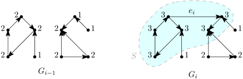
Figure 1. An example of a vertex weighting on $G_{i-1}$ and the updated weighting on $G_{i}$.

The weight of a vertex $v$ relates implicitly to the number of vertices that are images of $v$ in the copies of $G$ in $H_{t}$, where a higher weight means fewer copies (cf. Lemma 2.3 below). In particular, it counts how many times the random process must pick $v$ in order to create a copy of $G$ with an additional technical constraint that the weights cannot decrease along directed paths. The intuition is as follows. Suppose there is a number of images of $x_{i}$ lying within copies of $G_{i-1}$ in $H_{t}$. Only a fraction of them will become an image of $x_{i}$ in a copy of $G_{i}$, as the random process must choose them (assign a square) at a later time. Similarly, as the player assigns only one circle at a time, the pool of images of $y_{i}$ in copies of $G_{i}$ will shrink as the process progresses. Hereditarily, the same applies to the vertices further away from $x_{i}$ in $G_{i}$ but accessible from it by directed paths.

Lemma 2.2.

If $G$ has minimum degree $\delta=\delta(G)$ (where a loop edge $v\rightarrow v$ contributes one to the degree of $v$), then $w_{G}(v)\geq\delta$ for every vertex $v$.

Proof.

We prove the statement by induction on the number of edges $m=|E(G)|$. The base case is trivial. If $m=0$, then $G=G_{0}$, $\delta(G_{0})=0$, and all vertices have weight zero by definition.

For the inductive step, assume that $m\geq 1$ and the result holds for all graphs with fewer than $m$ edges. Let $\delta=\delta(G_{m})$. Clearly, $G_{m-1}$ has minimum degree $\delta$ or $\delta-1$. If $G_{m-1}$ has minimum degree $\delta$ then we are done, as $w_{G_{m}}(v)\geq w_{G_{m-1}}(v)\geq\delta$ for every vertex $v$.

Suppose then that $G_{m-1}$ has minimum degree $\delta-1$ and that $w_{G_{m-1}}(v)\geq\delta-1$ for all $v$. Let $e_{m}=x_{m}\rightarrow y_{m}$. We have $w_{G_{m}}(x_{m})=w_{G_{m-1}}(x_{m})+1\geq\delta$. Let $S$ be the set of all vertices $v$ where there is a directed path from $x_{m}$ to $v$ in $G_{m}$. We know that $x_{m}\in S$ (there is a degenerate directed path from $x_{m}$ to $x_{m}$) and $w_{G_{m}}(v)\geq w_{G_{m}}(x_{m})\geq\delta$ for any $v\in S$. If $S=V(G_{m})$ then we are done, so suppose not and let $T=V(G_{m})\setminus S$. Note that by definition there are no directed edges in $G_{m}$ from a vertex in $S$ to a vertex in $T$. (See Figure 1.) We construct a series of auxiliary graphs $T_{i}$ for $i=0,1,\ldots,m$ on vertex set $T$ as follows. Let $T_{0}$ be the empty graph on vertex set $T$. For each $1\leq i\leq m$, consider the edge $e_{i}=x_{i}\rightarrow y_{i}$ in $G_{m}$.

• If $x_{i},y_{i}\in T$ then let $T_{i}$ be $T_{i-1}$ with edge $x_{i}\rightarrow y_{i}$ added.

• If $x_{i}\in T,y_{i}\not\in T$, then let $T_{i}$ be $T_{i-1}$ with loop edge $x_{i}\rightarrow x_{i}$ added (with multiplicity if $x_{i}\rightarrow x_{i}$ is already included as an edge).

• Otherwise, if $x_{i}\not\in T$, let $T_{i}=T_{i-1}$.

These graphs naturally inherit the edge ordering from $G_{m}$.

Since $x_{m}\not\in T$, $e_{m}=x_{m}\rightarrow y_{m}$ is not added to $T_{m}$ and so we know that $T_{m}$ has strictly fewer than $m$ edges. We also have that $d_{T_{m}}(v)=d_{G_{m}}(v)$ for all $v\in T$, since there are no edges $e_{i}=x_{i}\rightarrow y_{i}$ with $x_{i}\not\in T$ and $y_{i}\in T$. (Indeed, suppose that $e_{i}=x_{i}\rightarrow y_{i}$ with $x_{i}\not\in T$ and $y_{i}\in T$. Since $x_{i}\not\in T$, $x_{m}\leadsto x_{i}$ in $G_{m}$ and so also $x_{m}\leadsto y_{i}$. We get $y_{i}\not\in T$ which gives us a contradiction. See Figure 1.) Thus by the inductive hypothesis, the weighting $w_{T_{m}}:T\rightarrow{\mathbb{N}}\cup\{0\}$ has $w_{T_{m}}(v)\geq\delta$ for all $v\in T$.

On the other hand, we can also show that $w_{T_{i}}(v)=w_{G_{i}}(v)$ for all $v\in T$ and all $i\leq m$. This certainly holds for $i=0$. If $e_{i}=x_{i}\rightarrow y_{i}$ with $x_{i}\in T$, then since there are no directed edges from $S$ to $T$ in $G_{m}$, we can see that adding $e_{i}$ to $G_{i-1}$ to get $G_{i}$ has the same impact on vertex weights within $T$ as adding the appropriate edge to $T_{i-1}$ to get $T_{i}$. For the same reason, if $x_{i}\not\in T$ then adding edge $e_{i}$ to $G_{i-1}$ to get $G_{i}$ has no effect on vertex weights within $T$. In particular, we obtain $w_{G_{m}}(v)=w_{T_{m}}(v)\geq\delta$ for all $v\in T$ and, consequently, $w_{G_{m}}(v)\geq\delta$ for all $v\in V(G_{m})$, since we already had that $w_{G_{m}}(v)\geq\delta$ for $v\in S=V(G_{m})\setminus T$. The proof of the lemma is finished. ∎

Recall that $H_{t}$ is the semi-random graph after $t$ time-steps. Before we can state our main lemma, we need to introduce a few more definitions. Let $G$ be an oriented graph with a fixed edge order $e_{1},e_{2},\ldots,e_{m}$. A homomorphism from $G$ to $H_{t}$ is a map that respects the edge orientations and edge ordering in the natural way. Formally, a homomorphism from $G$ to $H_{t}$ is an injective function $\phi:V(G)\rightarrow V(H_{t})$ such that: (a) if $e=u\rightarrow v$ is a directed edge in $G$ then $\phi(u)\rightarrow\phi(v)$ is a directed edge in $H_{t}$ which we call $\phi(e)$; and (b) for $i<j$, the edge $\phi(e_{i})$ was added to $H_{t}$ at an earlier time-step than the edge $\phi(e_{j})$. For a vertex $v\in V(G)$, define $S(v,G;t)$ to be the set of vertices $u$ in $H_{t}$ for each of which there is a homomorphism $\phi$ from $V(G)$ to $V(H_{t})$ such that $u=\phi(v)$.

We also need a notion of the diameter of an oriented graph. For any ordered pair of vertices $u,v\in G$ for which there exists directed path from $u$ to $v$, let $d(u,v)$ be the length of the shortest such path. Define $diam(G)$ to be the maximum value of $d(u,v)$ over all pairs $u,v$ with a directed path from $u$ to $v$. (We use the convention that $diam(G)=0$ if $G$ is the empty graph.) Note that $diam(G)\leq|V(G)|-1$ and that $diam(G)$ is not a monotone function of graphs.

Lemma 2.3.

Let $G$ be an oriented graph with a fixed edge order $(e_{1},\dots,e_{m})$, and let $w_{G}$ be the vertex weighting defined above. Then, for any strategy $\mathcal{S}$ of the player, any $t<n/2$, and any vertex $v\in V(G)$ with $w=w_{G}(v)$,

$$\mathbb{E}\ |S(v,G;t)|\leq\frac{t^{w}}{n^{w-1}}\left(2(w!)^{D}-1\right)$$

where $D=\max_{i}\{diam(G_{i})\}\leq|V(G)|-1$.

Proof.

We will prove a slightly stronger statement: for any vertex $v\in V(G)$ and any $i\in\{0,1,\ldots,m\}$,

$$\mathbb{E}\ |S(v,G_{i};t)|\leq\frac{t^{w_{i}(v)}}{n^{w_{i}(v)-1}}\left(2(w_{i}(v)!)^{D}-1\right),$$ (2.2)

where we use the shorthand $w_{i}=w_{G_{i}}$. The proof is by induction on $i$.

The base case is trivial. Indeed, if $i=0$, then by the definition of $w_{0}$ the weighting is identically zero. Clearly, for all $v\in V(G)$,

$$S(v,G_{0};t)=n=\frac{t^{0}}{n^{-1}}\left(2(0!)^{D}-1\right),$$

and so the desired inequality (2.2) holds.

For the inductive step, suppose that $i\geq 1$ and that (2.2) holds for $G_{i-1}$. We will show that it also holds for $G_{i}$. If $w_{i}(v)=0$, then clearly $|S(v,G_{i};t)|\leq n=\frac{t^{0}}{n^{-1}}\left(2(0!)^{D}-1\right)$ and we are done. If $w_{i}(v)=1$, then $v$ must be in some edge in $G_{i}$. If $v$ has a positive out-degree in $G_{i}$, then each vertex in $S(v,G_{i};t)$ has a positive out-degree in $H_{t}$. Otherwise, $v$ has a positive in-degree in $G_{i}$, and then each vertex in $S(v,G_{i};t)$ has a positive in-degree in $H_{t}$. Either way, $|S(v,G_{i};t)|\leq t=\frac{t^{1}}{n^{0}}\left(2(1!)^{D}-1\right)$ and we are done again.

Moreover, as, obviously,

$$|S(v,G_{i};t)|\leq|S(v,G_{i-1};t)|,$$

the result follows immediately for all vertices $v$ with $w_{i}(v)=w_{i-1}(v)$. Consequently, we only need to consider vertices $v$ where $w_{i}(v)\geq 2$ and $w_{i}(v)\neq w_{i-1}(v)$.

Let $e_{i}=x\rightarrow y$ and set $w_{i}(x)=w$. The condition $w_{i}(v)\neq w_{i-1}(v)$ only holds if there is a directed path from $x$ to $v$ in $G_{i}$, in which case $w_{i}(v)=w$ too. We will show by induction on the distance $d_{i}(x,v)$ from $x$ to $v$ in $G_{i}$ that

$$\mathbb{E}\ |S(v,G_{i};t)|\leq\frac{t^{w}}{n^{w-1}}\left(2w^{d_{i}(x,v)}\left((w-1)!\right)^{D}-1\right).$$ (2.3)

Since $d_{i}(x,v)\leq diam(G_{i})\leq D$, this will suffice to prove (2.2) and so to finish the proof of the lemma.

From now on we suppress the subscript $i$ in $d_{i}(x,y)$. First consider the case $d(x,v)=0$, that is, $v=x$. If $u\in S(x,G_{i};t)$, then there must be some time $t^{\prime}<t$ such that $u\in S(x,G_{i-1};t^{\prime})$ and $u$ was selected by the semi-random process at time $t^{\prime}+1$, when the image of the edge $e_{i}$ was added to create a copy of $G_{i}$. The probability that some vertex in $S(x,G_{i-1};t^{\prime})$ was selected by the semi-random process at time $t^{\prime}+1$ is $|S(x,G_{i-1};t^{\prime})|/n$. Thus,

$$\mathbb{E}\ |S(x,G_{i};t)|\leq\sum_{t^{\prime}=0}^{t-1}\frac{|S(x,G_{i-1};t^{\prime})|}{n}$$

and, by the linearity of expectation and (2.2), valid for $i-1$, we have

$$\mathbb{E}\ |S(x,G_{i};t)| \leq\sum_{t^{\prime}=0}^{t-1}\frac{\mathbb{E}\ |S(x,G_{i-1};t^{\prime})|}{n}$$

$$\leq\sum_{t^{\prime}=0}^{t-1}\frac{(t^{\prime})^{w-1}}{n\left(n^{w-2}\right)}\left(2\left((w-1)!\right)^{D}-1\right)$$

$$\leq\frac{t^{w}}{n^{w-1}}\left(2\left((w-1)!\right)^{D}-1\right),$$

as required.

Now, consider the case $d(x,v)>0$, that is, $v\neq x$ and there is a directed path from $x$ to $v$, and suppose that the hypothesis (2.3) holds for all $u$ with $d(x,u)<d(x,v)$. We fix a directed path from $x$ to $v$ of minimum length. Let $u$ be the vertex preceding $v$ on this path, so $d(x,u)=d(x,v)-1$. Observe that, by the definition of the weight function, $w_{i}(u)=w$.

The number of vertices in $S(v,G_{i};t)$ is bounded by the number of edges in $H_{t}$ which are the images of the edge $u\rightarrow v$ under some homomorphism $\phi$ from $G_{i}$ to $H_{t}$. We partition the vertices in $S(u,G_{i};t)$ into classes according to how many of the edges they are incident to are the images of $u\rightarrow v$ under some homomorphism. If a vertex in $S(u,G_{i};t)$ is incident to exactly $s$ such edges, then it contributes at most $s$ vertices to $S(v,G_{i};t)$.

Thus, the total contribution to $S(v,G_{i};t)$ from all vertices in $S(u,G_{i};t)$ that are incident to at most $w$ such edges is at most $w|S(u,G_{i};t)|$. On the other hand, the expected number of vertices in $S(u,G_{i};t)$ that are incident to exactly $s>w$ edges that are images of $u\rightarrow v$ is, by Lemma 2.1(a), at most $\frac{2t^{s}}{s!n^{s-1}}$. Combining these estimates, we have

$$\mathbb{E}\ |S(v,G_{i};t)| \leq w\mathbb{E}\ |S(u,G_{i};t)|+2\sum_{s\geq w+1}s\frac{t^{s}}{s!n^{s-1}}$$

$$\leq w\mathbb{E}\ |S(u,G_{i};t)|+\frac{2t^{w}}{w!n^{w-1}}\left(\frac{t}{n}+\frac{t^{2}}{n^{2}}+\ldots\right)$$

$$\leq w\frac{t^{w}}{n^{w-1}}\left(2w^{d(x,u)}\left((w-1)!\right)^{D}-1\right)+\frac{t^{w}}{n^{w-1}}\cdots\frac{t}{n-t},$$

since $w\geq 2$. It follows that

$$\mathbb{E}\ |S(v,G_{i};t)| \leq\frac{t^{w}}{n^{w-1}}\left(2w^{d(x,u)+1}\left((w-1)!\right)^{D}-w+\frac{t}{n-t}\right)$$

$$\leq\frac{t^{w}}{n^{w-1}}\left(2w^{d(x,v)}\left((w-1)!\right)^{D}-1\right),$$

as $t<n/2$. Thus, inequality (2.3) holds for all $v$ with a directed path from $x$ to $v$. This finishes the proof of the lemma. ∎

Now we combine the two lemmas to prove the theorem.

Proof of Theorem 1.2.

Let $G$ be a graph on $k$ vertices and $m$ edges with degeneracy $d$. Let $G^{\prime}$ be the (non-empty) $d$-core of $G$ so, in particular, $G^{\prime}$ has minimum degree at least $d$. We will show that, regardless of the strategy used by the player, a.a.s. $G^{\prime}$ is not a subgraph of $H_{t}$ as long as $t=o(n^{(d-1)/d})$. As a result, the same is true for $G\supseteq G^{\prime}$.

As mentioned at the beginning of this section, it is enough to show that the player cannot create a copy of $G$ following a specific (but arbitrarily chosen) orientation and order of the edges of $G$. Clearly, there are $2^{m}m!$ different configurations to select from (possibly a large constant, but it does not depend on $n$). We may consider $2^{m}m!$ auxiliary games, one for each configuration, on top of the regular game. Each game (both the auxiliary ones and the original one) is played by $2^{m}m!+1$ perfect players aiming to achieve their own respective goals. All the games are coupled in a natural way, that is, exactly the same squares are presented by the semi-random process to each of the players.

Fix an edge ordering and an orientation of the edges of $G$, and consider a perfect player playing the corresponding auxiliary game. Applying Lemma 2.2 to the $d$-core $G^{\prime}$ of $G$, we see that $w_{G^{\prime}}(v)\geq d$ for each vertex $v\in V(G^{\prime})$. Thus, by Lemma 2.3, for each vertex $v\in V(G^{\prime})$

$$\mathbb{E}\ |S(v,G^{\prime};t)|\leq\frac{t^{d}}{n^{d-1}}\left(2(d!)^{|V(G^{\prime})|-1}-1\right)=O\left(\frac{t^{d}}{n^{d-1}}\right).$$

Note that the above bound holds for all vertices $v\in V(G^{\prime})$. This property is slightly stronger than we need as we only need it for one vertex of $V(G^{\prime})$. Let us fix then an arbitrary vertex $v_{0}$ of $G^{\prime}$ and let $\omega=\omega(n)$ be any function that tends to infinity as $n\to\infty$. If $t=n^{(d-1)/d}/\omega$, then we have $\mathbb{E}\ |S(v_{0},G^{\prime};t)|=o(1)$ and so, by the first moment method, a.a.s. there are no vertices in $S(v_{0},G^{\prime};t)$. It follows that a.a.s. there is no copy of $G^{\prime}$, and thus of $G$, in $H_{t}$ with this given order and orientation of edges. In other words, the player playing this specific auxiliary game loses the game a.a.s.

This holds for every edge ordering and every orientation of the edges of $G$. As mentioned earlier, the number of such orderings and orientations is a constant depending only on $m=|E(G)|$. Thus, by the union bounds over all auxiliary games, a.a.s. all players playing auxiliary games lose their own respective games. It follows that a.a.s. a perfect player playing the original game loses too (if not, the other players could all copy the same strategy, and one of them would win her game). The proof is finished. ∎

3. Proofs for hypergraphs when $r=1$

In the case when $r=1$, the semi-random process for hypergraphs has that in each step $t$, a single vertex $u_{t}$ is chosen uniformly at random from $[n]$, the same as for the process on graphs. The player then replies by selecting a set of $s-1$ vertices $V_{t}$ and the edge $\{u_{t}\}\cup V_{t}$ is added.

The proofs of Theorems 1.4 and 1.5 follow the same approach as in the graph case considered in Section 2 and, therefore, we only sketch them here emphasizing the required differences. The proof of Theorems 1.4 is again based on Lemma 2.1 and, indeed, proceeds mutatis mutandis.

Proof of Theorem 1.4.

Follow the same approach as in the proof of Theorem 1.2, dividing the process into phases where in each phase, the next vertex according to the degeneracy ordering is added. The only difference in this case is that in each phase, we must create all edges in which the new vertex is the last vertex rather than all edges, but since $r=1$ these can be constructed in exactly the same way. ∎

Now we outline the proof of Theorem 1.5 by discussing the necessary changes in the proof of the graph counterpart. Let $G$ be a hypergraph on $k$ vertices and $m$ edges that is not necessarily uniform and may contain parallel edges (allowing these cases will be useful in the proof of Lemma 3.1). Fix an ordering of the edges $(e_{1},e_{2},\ldots,e_{m})$ of $G$, and for each edge $e_{i}$ fix a leading vertex $x_{i}$. Given such a $G$, define an auxiliary graph $graph(G)$ on the same vertex set $V$ where for each edge $e_{i}\in G$, we have that $graph(G)$ contains the directed edges $x_{i}\rightarrow u$ for every $u\in e_{i}\setminus\{x_{i}\}$.

As in the graph case, we recursively define a weight function $w_{G}:V\rightarrow{\mathbb{N}}\cup\{0\}$ on the vertices of $G=(V,E)$ that is dependent on the edge order and choice of leading vertices. Let $G_{0}$ be the empty hypergraph on vertex set $V$ and define the weighting $w_{G_{0}}:V\rightarrow{\mathbb{N}}\cup\{0\}$ to be uniformly zero. For $1\leq i\leq m=|E|$, let $G_{i}$ have vertex set $V$ and edge set $\{e_{1},e_{2},\ldots,e_{i}\}$ (so $G_{m}=G$). In particular, $G_{i}$ is $G_{i-1}$ with edge $e_{i}$ added. Define $w_{G_{i}}:V\rightarrow{\mathbb{N}}\cup\{0\}$ by

$$w_{G_{i}}(x_{i})=w_{G_{i-1}}(x_{i})+1$$

and for all other vertices $v$,

$$w_{G_{i}}(v)=\begin{cases}\max\{w_{G_{i}}(x_{i}),w_{G_{i-1}}(v)\}&\text{if $x_{i}\leadsto v$ in $graph(G_{i})$}\\ w_{G_{i-1}}(v)&\text{otherwise,}\end{cases}$$

where $x_{i}\leadsto v$ denotes that there is a directed path from $x_{i}$ to $v$.

Lemma 3.1.

If $G$ has minimum degree $\delta=\delta(G)$, then $w_{G}(v)\geq\delta$ for every vertex $v$.

Proof.

The proof follows the same approach as the proof of Lemma 2.2, using induction on the number of edges $m=|E(G)|$. ∎

Let $H_{t}=H_{t}^{(1,s)}$ be the semi-random hypergraph after $t$ time-steps and let $u_{t}$ be the single vertex in the randomly chosen set $U_{t}$ at time $t$. Before we can state our main lemma we need to generalize some of our earlier definitions to hypergraphs. Let $G$ be an hypergraph with a fixed edge order $e_{1},e_{2},\ldots,e_{m}$ where each edge $e_{i}$ is assigned a leading vertex $x_{i}\in e_{i}$. A homomorphism from $G$ to $H_{t}$ is a map that respects the leading vertices and edge ordering in the natural way (analogously to the graph case). For a vertex $v\in V(G)$, define $S(v,G;t)$ to be the set of vertices in $H_{t}$ which are the image $\phi(v)$ for some homomorphism $\phi$ from $V(G)$ to $V(H_{t})$. We also define the diameter $diam(G)$ of the hypergraph to be the diameter of the auxiliary graph $graph(G)$, in the same sense as defined in Section 2.

Lemma 3.2.

Let $G$ be an hypergraph with a fixed edge order $e_{1},e_{2},\ldots,e_{m}$ where each edge $e_{i}$ is assigned a leading vertex $x_{i}\in e_{i}$. Let $w_{G}$ be the vertex weighting defined above. Then, for any strategy $\mathcal{S}$ of the player, any $t<n/2$, and any vertex $v\in V(G)$ with $w=w_{G}(v)$,

$$\mathbb{E}\ |S(v,G;t)|\leq\frac{t^{w}}{n^{w-1}}k\left(2(w!)^{D}-1\right)$$

where $D=\max_{i}\{diam(G_{i})\}\leq|V(G)|-1$.

Proof.

The proof of this Lemma follows the exact same approach as the proof of Lemma 2.3. Specifically, one can show by induction on $i$ that if hypergraph $G$ has $m$ edges then for any vertex $v\in V(G)$ and any $i\in\{0,1,\ldots,m\}$,

$$\mathbb{E}\ |S(v,G_{i};t)|\leq\frac{t^{w}}{n^{w-1}}k\left(2(w!)^{D}-1\right),$$

where $w=w_{G_{i}}(v)$. The only change needed in the proof is to use the directed paths given by the auxiliary graphs $graph(G_{i})$, whereas in the original proof the $G_{i}$’s were themselves oriented. ∎

Now we combine the two lemmas to prove the lower bound.

Proof of Theorem 1.5.

Let $G$ be a hypergraph on $k$ vertices and $m$ edges with degeneracy $d$. Let $G^{\prime}$ be the (non-empty) $d$-core of $G$ so, in particular, $G^{\prime}$ has minimum degree at least $d$.

Using the same coupling argument as in the proof of Theorem 1.2 one can see that, regardless of the strategy used by the player, a.a.s. $G^{\prime}$ is not a sub-hypergraph of $H_{t}$ as long as $t=o(n^{(d-1)/d})$. As a result, the same is true for $G\supseteq G^{\prime}$. ∎

4. Proofs for hypergraphs when $r\geq 2$

Here we prove Theorems 1.7 and 1.9 as well as some related results.

4.1. Lower Bound

Let us recall the statement of the theorem.

Theorem 1.7.

Let $k\geq s\geq r\geq 2$, and let $G$ be an $s$-uniform hypergraph with $k$ vertices and $m$ edges. Then, for any strategy $\mathcal{S}$ we have that

$$\lim_{n\to\infty}\mathbb{P}[H^{(r,s)}_{t}\in\mathcal{P}_{G}]=0,$$

where $t=n^{r-(k-s+r)/m}/\omega$ and $\omega=\omega(n)$ is any function tending to infinity as $n\to\infty$. As a result, $\tau^{(r)}_{\mathcal{P}_{G}}\geq r-(k-s+r)/m$.

Proof.

Set $H_{t}:=H_{t}^{(r,s)}$. This generic proof relies on an obvious observation that for a copy of $G$ to exist in $H_{t}$, there must be, in the first place, a set of $k$ vertices spanning at least $m$ edges of $H_{t}$. Formally, for any $j$, $1\leq j\leq m$, any time $t$, and any strategy $\mathcal{S}$, let $X_{j}^{\mathcal{S}}(t)$ be a random variable counting the number of $k$-element sets of vertices that induce in $H_{t}$ at least $j$ edges at the end of round $t$. We will assume that the player plays according to a strategy $\mathcal{S}$. However, since we only provide a universal upper bound for the expected value of $X_{j}^{\mathcal{S}}(t)$, it will actually not depend on $\mathcal{S}$. As a result, to unload the notation a little bit, let us suppress the dependence on the strategy $\mathcal{S}$.

We will show by induction on $j$ that for any $1\leq j\leq m$ we have

$$\mathbb{E}X_{j}(t)\leq t^{j}k^{r(j-1)}n^{k-s+r-rj}\qquad\qquad\mbox{for all }\;t\geq 1.$$ (4.1)

The base case $j=1$, holds trivially and deterministically, as we have

$$X_{1}(t)\leq t\binom{n-s}{k-s}\leq tn^{k-s}.$$

Indeed, there are precisely $t$ edges at the end of round $t$, and each of them is contained in $\binom{n-s}{k-s}$ sets of size $k$ (as we are after an upper bound, we ignore the possible repetitions of the $k$-sets here).

For the inductive step, suppose that (4.1) holds for some value of $j-1$, $1\leq j-1<m$ (and all $t$) and our goal is to show that it holds for $j$ too (again, for all $t$). We say that a set $W\subseteq[n]$, $|W|=k$, is of type $j$ at time $t$ if it spans in $H_{t}$ at least $j$ edges and we define an indicator random variable $I_{j}^{W}(t)$ equal to 1 if $W$ is of type $j$ at time $t$, and 0 otherwise. Thus (as a sanity check),

$$X_{j}(t)=\sum_{W\in\binom{[n]}{k}}I_{j}^{W}(t).$$ (4.2)

Note that in order to create a set $W$ of type $j$ at time $i$, it is necessary that $W$ is of type $j-1$ at time $i-1$ (in fact, having exactly $j-1$ edges), as well as, the $r$-vertex set selected by the semi-random hypergraph process at time $i$ is contained in $W$, that is, $U_{i}\subseteq W$. Thus, setting also $J^{W}(t)=1$ if $U_{t}\subseteq W$ and 0 otherwise, we have

$$X_{j}(t)\leq\sum_{i=1}^{t}\sum_{W\in\binom{[n]}{k}}I_{j-1}^{W}(i-1)J^{W}(i).$$ (4.3)

Since $U_{i}$ is selected uniformly at random from $\binom{[n]}{r}$,

$$\mathbb{E}(J^{W}(i))=\mathbb{P}(J^{W}(i)=1)=\frac{\binom{k}{r}}{\binom{n}{r}}.$$

We now take the expectation on both sides of (4.3). Using the linearity of expectation, independence of $I_{j-1}^{W}(i)$ and $J^{W}(i)$, (4.2), and the fact that the right hand side of (4.1) is an increasing function of $t$, we get that

$$\mathbb{E}X_{j}(t) \leq \sum_{i=1}^{t}\ \mathbb{E}\left(\sum_{W\in\binom{[n]}{k}}I_{j-1}^{W}(i-1)\right)\frac{\binom{k}{r}}{\binom{n}{r}}~{}~{}=~{}~{}\sum_{i=1}^{t}\ \mathbb{E}X_{j-1}(i-1)\frac{\binom{k}{r}}{\binom{n}{r}}$$

$$\leq t\cdot\left(t^{j-1}k^{r(j-1-1)}n^{k-s+r-r(j-1)}\right)\cdot\frac{k^{r}}{n^{r}}~{}~{}\leq~{}~{}t^{j}k^{r(j-1)}n^{k-s+r-rj},$$

and so (4.1) holds for $j$ too. This finishes the inductive proof of (4.1).

The desired conclusion is now easy to get. Note that, by (4.1) with $j=m$,

$$\mathbb{E}X_{m}(t)\leq t^{m}k^{r({m}-1)}n^{k-s+r-r{m}}=O\left(n^{k-s+r}\left(\frac{t}{n^{r}}\right)^{m}\right).$$

Hence, if $t=o(n^{r-(k-s+r)/{m}})$, then $\mathbb{E}X_{m}(t)=o(1)$ and so by the first moment method $X_{m}(t)=0$ a.a.s. Since creating a copy of $G$ in $H_{t}$ implies that $X_{m}(t)\geq 1$, we conclude that a.a.s. $H^{(r,s)}_{t}\not\in\mathcal{P}_{G}$ which was to be proved. ∎

4.2. Exact Thresholds for Starpluses

In this subsection we prove Theorem 1.9. However, we give a detailed proof only in the special case when $c=s-r=1$, followed by a short outline for the general case, which is very similar but more cumbersome.

Recall that an $s$-graph is a full 1-star if its edge set consists of all $s$-tuples containing a fixed vertex $v$, and an $(s,1)$-starplus, or just $s$-starplus of excess $\ell$ is any $s$-graph obtained from a full star by adding to it $\ell$ edges. We first restate Theorem 1.9 in this special case.

Theorem 4.1.

Let $r\geq 2$, $s=r+1$, and let $G$ be an $s$-starplus on $k\geq s$ vertices and excess

$$\ell\leq\frac{r\binom{k-1}{r}-(k-1)}{k-1-r}.$$

Then, there exists a strategy $\mathcal{S}$ such that

$$\lim_{n\to\infty}\mathbb{P}[H_{t}^{(r,s)}\in\mathcal{P}_{G}]=1,$$

where $t=n^{r-(k-1)/\left(\binom{k-1}{r}+\ell\right)}\omega$ and $\omega=\omega(n)$ is any function tending to infinity as $n\to\infty$. As a result,

$$\tau^{(r)}_{\mathcal{P}_{G}}=r-\frac{k-1}{\binom{k-1}{r}+\ell}.$$

Proof.

For an integer $s\geq 3$, let $G$ be an $s$-uniform starplus on $k\geq s$ vertices and excess

$$\ell\leq L:=\frac{r\binom{k-1}{r}-(k-1)}{k-1-r},$$

where $r=s-1$. We call the $\ell$ edges not containing the center of the star in $G$ the surplus edges. Set

$$m=|E(G)|=\binom{k-1}{r}+\ell\;,\quad\kappa=r-\frac{k-1}{m}\;,\quad\mbox{and}\quad t=\omega n^{\kappa},$$

where $\omega:=\omega(n)\to\infty$ as $n\to\infty$ but, say, $\omega=o(\log n)$.

Let us again abbreviate $H_{t}:=H_{t}^{(s-1,s)}$. To play the game ${\mathcal{P}}_{G}$, we equip the player with the following strategy. The vertex $n$ is put aside. From the player’s point of view there will be two phases of the game (but just one for $\ell=0$), lasting, respectively, $t_{1}$ and $t_{2}:=t-t_{1}$ steps, where

$$t_{1}=\begin{cases}t\quad\mbox{ when }\ell=0\\ t/2\mbox{ when }1\leq\ell<L\\ \epsilon t\;\;\;\mbox{ when }\ell=L,\end{cases}$$

and

$$\epsilon=\omega^{-1-\frac{\ell}{2\binom{k-1}{r}}}.$$

In the last case it will be convenient to write

$$t_{1}=\frac{n^{\kappa}}{\omega_{1}},\quad\mbox{where}\quad\omega_{1}=\omega^{\frac{\ell}{2\binom{k-1}{r}}}.$$

During the first phase, whenever a random $r$-set $U_{i}$ lands within $[n-1]$, the player draws the edge $U_{i}\cup\{n\}$, that is, $V_{i}=\{n\}$. The goal of this phase is to collect sufficiently many edge-disjoint copies of $K_{k-1}^{r}$ created by the random $r$-sets $U_{i}$. Due to the player’s strategy, this will yield in $H_{t_{1}}$ plenty of copies of the $s$-uniform full star on $k$ vertices with the same center, namely, the vertex $n$. This will end the proof when $\ell=0$.

For $\ell\geq 1$, in order to turn at least one of the stars into a copy of the starplus $G$, one of the edge-disjoint copies of $K_{k-1}^{r}$ obtained in phase one has to be hit by at least $\ell$ random $r$-sets which, collectively, should be extendable (by the player) to a copy of $G$. To this end, in each such copy of $K_{k-1}^{r}$, we designate $\ell$ $r$-sets (with possible, and sometimes necessary, repetitions) such that their suitable extensions to $s$-sets lead to a copy of $G$. This can be easily done by selecting an arbitrary $r$-element subset of each surplus edge of $G$ (see Figure 2 for an example). During the second phase, whenever a random $r$-set lands on one of the designated $r$-sets, the player draws the respective edge (owing to the edge-disjointness of the copies of $K_{k-1}^{(r)}$, there is no ambiguity here).

For this strategy to be a.a.s. successful, we need to study the behaviour of three random variables. Let $X$ be a random variable counting the number of copies of $K_{k-1}^{r}$ created randomly during the first phase on the set $[n-1]$. Here we identify the copies with their vertex sets, thus making multiple edges irrelevant.

Let $\mathcal{K}$ be the family of copies of $K_{k-1}^{r}$ counted by $X$ and let $Y$ be the number of pairs of copies in $\mathcal{K}$ which share at least one edge (that is, an $r$-set). Further, let $\mathcal{K}^{\prime}$ be a family of copies of $K_{k-1}^{r}$ obtained by removing from $\mathcal{K}$ at least one copy from each pair counted by $Y$.

Finally, let $Z$ be the number of copies of $G$ at the end of the second phase whose vertex sets consist of the vertex $n$ together with the vertex set of one of the copies of $K_{k-1}^{r}$ in $\mathcal{K}^{\prime}$. Our ultimate goal is to show that a.a.s. $Z>0.$ To achieve it, we will first need to prove that a.a.s. $\mathcal{K}^{\prime}$ is sufficiently large. This will boil down, in turn, to showing that $X$ is sufficiently large, while $Y=o(X)$.

Let us begin with the expectation of $X$. We denote by $R_{t_{1}}$ the (random) multi-$r$-graph on vertex set $[n-1]$ consisting of all sets $U_{i}$, $i=1,\dots,t_{1}$, which do not contain vertex $n$. To better understand the forthcoming estimates, let us first consider a small special case: $r=2$ and $k=4$. Then $X$ counts triangles in $R_{t_{1}}$, disregarding multiple edges (e.g., if there are edges 12, 13, 23, and 12 has multiplicity 2, then we still have just one triangle on vertices $1,2,3$, not two). There are $\binom{n-1}{3}$ triangles in $K_{n-1}$ on $[n-1]$. Let us fix one, say, $T=123$. Let $t_{ij}$ be the first time the pair $ij$ is hit by the random process. Assuming $1\leq t_{12}<t_{13}<t_{23}\leq t_{1}$, we then have

$$\mathbb{P}(T\subseteq R_{t_{1}})=\left(1-\frac{3}{\binom{n}{2}}\right)^{t_{12}-1}\times\left(1-\frac{2}{\binom{n}{2}}\right)^{t_{13}-t_{12}-1}\times\left(1-\frac{1}{\binom{n}{2}}\right)^{t_{23}-t_{13}-1}\times\left(\frac{1}{\binom{n}{2}}\right)^{3}.$$

As the product of the first three factors is squeezed between 1 and $(1-3/\binom{n}{2})^{t_{1}}$, it converges to 1, since $t_{1}=o(n^{r})$ and $r=2$ here. Thus, in this case, by considering all $\binom{n-1}{3}$ triangles in $K_{n-1}$, all $3!$ orderings of $t_{12},t_{13},t_{23}$ and all $\binom{t_{1}}{3}$ their choices, we have, by symmetry,

$$\mathbb{E}X=\binom{n-1}{3}\times t_{1}(t_{1}-1)(t_{1}-2)\times\mathbb{P}(T\subseteq R_{t_{1}})\sim\binom{n-1}{3}\left(\frac{t_{1}}{\binom{n}{2}}\right)^{3}.$$

In general, by similar calculations, setting $p_{1}=\frac{t_{1}}{\binom{n}{r}}$,

$$\mathbb{E}X\sim\binom{n-1}{k-1}p_{1}^{\binom{k-1}{r}}=\begin{cases}\Theta\left(\omega^{\binom{k-1}{r}}n^{(k-1)\ell/m}\right)\quad\mbox{when}\quad 0\leq\ell<L\\ \Theta\left(\omega_{1}^{-\binom{k-1}{r}}n^{(k-1)\ell/m}\right)\quad\mbox{when}\quad\ell=L.\end{cases}$$ (4.4)

We are now going to apply the second moment method as described in the proof of Lemma 2.1 in Section 2.1, based on inequality (2.1). Since $\mathbb{E}X\to\infty$ as $n\to\infty$, it again suffices to show that $\mathbb{E}(X(X-1))\sim(\mathbb{E}X)^{2}$. To this end, we categorize the (ordered) pairs of cliques $K_{k-1}^{(r)}$ in $R_{t_{1}}$ according to the size of their vertex-intersection $q$, $0\leq q\leq k-2$, and write, by symmetry,

$$\mathbb{E}(X(X-1))=\sum_{q=0}^{k-2}\binom{n-1}{k-1}\binom{k-1}{q}\binom{n-k}{k-1-q}\mathbb{P}(K_{1}\cup K_{2}\subseteq R_{t_{1}}),$$

where $K_{1},K_{2}$ is an arbitrary pair of cliques $K_{k-1}^{(r)}$ in $R_{t_{1}}$ which share exactly $q$ vertices. By similar estimates as before, fixing the order of appearance of the $2\binom{k-1}{r}-\binom{q}{r}$ edges of $K_{1}\cup K_{2}$ and the times they appear for the first time in $R_{t_{1}}$, we get

$$\mathbb{P}(K_{1}\cup K_{2}\subseteq R_{t_{1}})\sim p_{1}^{2\binom{k-1}{r}-\binom{q}{r}}.$$

Returning to the estimate of $\mathbb{E}(X(X-1))$, we see that the term corresponding to $q=0$,

$$\binom{n-1}{k-1}\binom{n-k}{k-1}p_{1}^{2\binom{k-1}{r}}\sim(\mathbb{E}X)^{2},$$

while, recalling the definitions of $p_{1}$ and $t_{1}$,

$$\frac{1}{(\mathbb{E}X)^{2}}\sum_{q=1}^{k-2}\binom{n-1}{k-1}\binom{k-1}{q}\binom{n-k}{k-1-q}p_{1}^{2\binom{k-1}{r}-\binom{q}{r}}=\Theta\left(\sum_{q=1}^{k-2}\frac{1}{n^{q}p_{1}^{\binom{q}{r}}}\right)=o(1).$$

(To see the last equality notice that $q\binom{k-1}{r}>(k-1)\binom{q}{r}$ and the lower order terms, $\omega$ or $\omega_{1}$ are negligible here.) Hence, in particular, a.a.s.

$$\frac{1}{2}\mathbb{E}X\leq X\leq\frac{3}{2}\mathbb{E}X$$ (4.5)

and so, a.a.s. the right hand side of (4.4) sets bounds on $X$ as well. This completes the proof in the case $\ell=0$, that is, when $G$ is a genuine star.

Now assume that $\ell\geq 1$ and turn to the random variable $Y$. Its expectation coincides with the part of the formula for $\mathbb{E}(X(X-1))$ corresponding to $q\geq r$, that is,

$$\mathbb{E}Y=\mathbb{E}X\times O\left(\sum_{q=r}^{k-2}n^{k-1-q}p_{1}^{\binom{k-1}{q}-\binom{q}{r}}\right),$$

after pulling out $\mathbb{E}X$. We want to show that $n^{k-1-q}p_{1}^{\binom{k-1}{r}-\binom{q}{r}}=o(1)$ for each $q=r,\dots,k-2$. Recalling, again, the definitions of $p_{1}$ and $t_{1}$, let us focus on the (hidden) exponent of $n$ in this expression, that is,

$$k-1-q-\frac{k-1}{m}\left[\binom{k-1}{r}-\binom{q}{r}\right].$$

We are going to show that it is non-positive and, in fact, in all cases but when $q=r$ and $\ell=L$, strictly negative. The non-positivity of it is equivalent to the inequality

$$\ell\leq\frac{q\binom{k-1}{r}-(k-1)\binom{q}{r}}{k-1-q}:=f(q).$$

Note that $f(r)=L$, which means that if $\ell=L$, then the factor of $n$ vanishes but fortunately, we have the $\omega_{1}$ in the denominator which does the job (this is the sole reason, in fact, why we have changed the definition of $t_{1}$ when $\ell=L$). More precisely, in that case we have

$$n^{k-1-r}p_{1}^{\binom{k-1}{r}-1}=O\left(\omega_{1}^{-\binom{k-1}{r}+1}\right)=o(1).$$

We will now show that $f(q)$ is a strictly increasing function of $q=r,\dots,k-2$. Indeed, for $r\leq q\leq k-3$, the inequality $f(q)<f(q+1)$ is, after some tedious but elementary transformations, equivalent to

$$(k-1-q)\binom{q}{r-1}+\binom{q}{r}<\binom{k-1}{r}.$$

The last inequality can be easily verified by counting the number of $r$-element subsets of $[k-1]$ with at most one element outside $[q]$. In summary, for all cases when $q>r$ or $\ell<L$ the exponent of $n$ is strictly negative and, regardless of whether $\ell=L$ or $\ell<L$, there is a sequence $\gamma(n)\to 0$ such that $\mathbb{E}Y=O(\gamma(n)\mathbb{E}X)$ and so, by Markov’s inequality, a.a.s. $Y=O(\sqrt{\gamma(n)}\mathbb{E}X)$ and, in view of (4.5), a.a.s. $Y=o(X)$. Consequently, a.a.s.

$$|{\mathcal{K}}^{\prime}|=(1-o(1))X$$

and the right hand side of (4.4) applies to $|{\mathcal{K}}^{\prime}|$ as well.

Next, we move to the second phase of the process. Let $K_{1},\dots,K_{|{\mathcal{K}}^{\prime}|}$ be the copies of $K_{k-1}^{(r)}$ belonging to ${\mathcal{K}}^{\prime}$. In the starplus $G$, for each of the $\ell$ surplus edges, we fix one $r$-element subset. The obtained set of $\ell$, not necessarily distinct, $r$-sets forms a multi-$r$-graph which we denote by $M$; see Figure 2. For each $i=1,\dots,|{\mathcal{K}}^{\prime}|$, let us fix an arbitrary copy $M_{i}$ of $M$ within $K_{i}$. Further, set $R_{t_{2}}$ to be the random $r$-graph consisting of the random $r$-sets $U_{i}$, $i=t_{1}+1,\dots,t$, and let $I_{i}=1$ if $M_{i}\subseteq R_{t_{2}}$ and $I_{i}=0$ otherwise. Then, $Z=\sum_{i=1}^{|{\mathcal{K}}^{\prime}|}I_{i}$ and our goal is to prove that a.a.s. $Z>0$.

Figure 2. A 3-uniform starplus on 8 vertices with surplus edges forming the Fano plane (the 21 edges containing $v$ are not shown). The red pairs indicate a possible choice of the graph $M$ (one of $3^{7}$). In this particular case, obviously, $M$ cannot be a multigraph.

We again apply the second moment method. The quantity $\mathbb{E}I_{i}=\mathbb{P}(M_{i}\subseteq R_{t_{2}})$ is the same for each $i$. To estimate it, we use the same approach as before, except that now we may have parallel edges. Let us again consider first a small example. Let $T^{\prime}$ be the triangle on $123$ with the edge 12 doubled. If, say, the times of hitting particular edges are fixed at $t_{1}+1\leq t_{13}<t_{12}<t_{23}<t_{12}^{\prime}\leq t$, then the probability of actually hitting $T^{\prime}$ at these times is

$$\left(1-\frac{3}{\binom{n}{2}}\right)^{t_{13}-1}\left(1-\frac{2}{\binom{n}{2}}\right)^{t_{12}-t_{13}-1}\left(1-\frac{2}{\binom{n}{2}}\right)^{t_{23}-t_{12}-1}\left(1-\frac{1}{\binom{n}{2}}\right)^{t_{12}^{\prime}-t_{23}-1}\left(\frac{1}{\binom{n}{2}}\right)^{4}.$$

And the number of ways to select the four times is, due to exchangeability of $t_{12}$ and $t_{12}^{\prime}$, not $4!$ but $4!/2$. Thus,

$$\mathbb{E}I_{i}\sim\frac{4!}{2}t_{2}^{4}\left(\frac{1}{\binom{n}{2}}\right)^{4}\sim\frac{4!}{2}\left(\frac{t}{\binom{n}{2}}\right)^{4};$$

recall that $t_{2}=t-t_{1}$ is the length of the second phase. Similarly, in the general case, setting $p_{2}=\frac{t_{2}}{\binom{n}{r}}$ and denoting by $\ell_{1},\dots,\ell_{h}$, where $\ell_{1}+\cdots+\ell_{h}=\ell$, the multiplicities of edges in $M$, we obtain, using also (4.4),

$$\mathbb{E}Z=|{\mathcal{K}}^{\prime}|\mathbb{E}I_{1}\sim|{\mathcal{K}}^{\prime}|\frac{p_{2}^{\ell}}{\ell_{1}!\cdots\ell_{h}!}=\begin{cases}\Theta\left(\omega^{\binom{k-1}{r}+\ell}\right)\quad\mbox{when}\quad 1\leq\ell<L\\ \Theta\left(\omega_{1}^{-\binom{k-1}{r}}\omega^{\ell}\right)=\Theta\left(\omega^{\ell/2}\right)\quad\mbox{when}\quad\ell=L.\end{cases}$$

(In fact, the choice of $\omega_{1}$ has been driven by this very calculation.)

We now apply the same version of the second moment method as was before applied to $X$. However, since $\mathbb{E}Z\to\infty$ as $n\to\infty$ and, unlike before, the copies $M_{1},\dots,M_{|{\mathcal{K}}^{\prime}|}$ of $M$ are edge-disjoint (and the number of common vertices does not matter), we easily get the estimate

$$\mathbb{E}(Z(Z-1))\sim|{\mathcal{K}}^{\prime}|^{2}\frac{p_{2}^{2\ell}}{l_{1}!^{2}\cdots\ell_{j}!^{2}}\sim\mathbb{E}Z.$$

So, by Chebyshev’s inequality, a.a.s., $Z\geq\tfrac{1}{2}\mathbb{E}Z$, which completes the proof. ∎

Proof of Theorem 1.9 (outline).

The proof follows practically the same 2-phase strategy as the above proof of Theorem 4.1. Here we put aside a set $C^{\prime}$ of $s-r$ vertices and, in phase one, on the remaining $n-(s-r)$ vertices, create many cliques $K_{k-(s-r)}^{(r)}$. If an $r$-set contained in $[n]\setminus C^{\prime}$ is hit, the player extends it to an $s$-element edge by adding to it the set $C^{\prime}$. Phase two is mutatis mutandis the same as in the proof of Theorem 4.1, except that among the $\ell$ missing edges we have to add to a copy of $K_{k-(s-r)}^{(r)}$ there are some which intersect (but do not contain) the set $C^{\prime}$. This, however, does not cause any problems. The probabilistic analysis is very similar and therefore is omitted too. ∎

4.3. Miscellaneous Results

Here we gather various further results related to Theorems 1.7 and 1.9.

4.3.1. Starpluses with non-full stars

One might generalize Theorem 1.9 to
starpluses whose stars are not full. Instead of attempting to formulate a general result, we will focus here only on the case $r=s-1$ and consider an example of a class of hypergraphs for which such an approach turned out to be successful.

An $s$-uniform $\ell_{1}$-partial starplus with excess $\ell_{2}$ is an $s$-graph $G$ which is a union of a star $G_{1}$ with center $v$ and $\ell_{1}$ edges and an arbitrary $s$-graph $G_{2}$ on vertex set $V(G)\setminus\{v\}$ with $\ell_{2}$ edges. (So, in fact, every $s$-graph can be viewed as a partial starplus.) Using the same ideas as in the proof of Theorem 4.1, one can prove a similar result establishing, under some symmetry assumptions on the structure of $G_{1}$, an upper bound on $\tau^{(r)}_{\mathcal{P}_{G}}$ which matches the lower bound in Theorem 1.7, provided

$$\frac{\ell_{1}+\ell_{2}}{\ell_{2}-1}\leq\frac{k-1}{k-1-r}.$$

An example of a partial starplus for which this approach works is the wheel $G=W_{k}^{(s)}$ where $G_{2}$ is a tight $s$-cycle $(u_{1}\dots,u_{k-1})$ on $V(G)\setminus\{v\}$ (for the definition see Subsection 1.2) and the star $G_{1}$ consists of all $k-1$ edges containing $v$ and a consecutive $(s-1)$-segment of $G_{2}$. So, the neighborhoods of $v$ form a tight $r$-cycle, $r=s-1$. It can be easily checked that in this case, as $\ell_{1}=\ell_{2}=k-1$, the above inequality is satisfied whenever $r=s-1\geq k/2$, and then $\tau^{(r)}_{\mathcal{P}_{G}}=r-1/2$.

4.3.2. The clique $K_{6}^{(3)}$

There are a whole lot of cases when the assumption (1.2) on $\ell$ is not met. Still, using some ad-hoc modifications of our approach one can often get upper bounds on $\tau^{(r)}_{\mathcal{P}_{G}}$ which are not too far from the lower bound set by Theorem 1.7. As a pivotal illustration, consider the clique $G=K_{6}^{(3)}$ and $r=s-1=2$. By Theorem 1.7 and Corollary 1.10 we already know that $\tfrac{7}{4}\leq\tau^{(2)}_{\mathcal{P}_{G}}\leq\tfrac{20}{11}$. By modifying the strategy used in the proof of Theorem 4.1, one can improve the upper bound a little.

Proposition 4.2.

$\tau^{(2)}_{\mathcal{P}_{K_{6}^{(3)}}}\leq\tfrac{9}{5}$

Proof (outline).

Consider the following version of the strategy used previously. In essence, we alter how the edge set of $K_{6}^{(3)}$ is split between phase one and phase two. We put aside two vertices, say $n-1$ and $n$, and in phase one the first time a $2$-element subset $S$ of $[n-2]$ is randomly selected, it is extended by the player to the $3$-edge $S\cup\{n-1\}$, while if it is a second hit, it is extended to $S\cup\{n\}$. So in $R_{t_{1}}$, we are after the double cliques on four vertices, that is, complete 4-vertex multigraphs where each edge appears twice. Set $t=\omega n^{9/5}$ and $t_{1}=n^{9/5}/\sqrt{\omega}$, where $\omega=\omega(n)$ is any function such that $\lim_{n\to\infty}\omega(n)=\infty$ and, for convenience, $p=t/\binom{n}{2}$ and $p_{1}=t_{1}/\binom{n}{2}$. Then, by the second moment method (details omitted) there are a.a.s. $\Theta(n^{4}p_{1}^{12})$ double $K_{4}$’s, and luckily most of them are edge-disjoint. This is because the expected number of extensions of a given double clique that contain one of its (double) edges is $\Theta(n^{2}p_{1}^{10})=o(1)$.

To see what happens in the second phase, consider one of the selected copies of the double clique, say on vertices $1,2,3,4$. When during the process $R_{t_{2}}$ a pair $\{j,j+1\}$ is hit, $j=1,\dots,4$, the player extends it to $\{j,j+1,j+2\}$ (here $5:=1$ and $6:=2$), that is, by adding the next vertex along the cycle $12341$. (In the notation of the proof of Theorem 4.1, we would have $M=\{12,23,34,14\}$.)

However, we still need 4 more edges to complete a copy of $K_{6}^{(3)}$. To this end, for the first time a pair $(j,n-i)$ is hit, $j=1,\dots,4$, $i=1,2$, the player extends it to $\{j,n-1,n\}$. The expected number of copies of $K_{6}^{(3)}$ obtained this way is thus $\Theta(n^{4}p_{1}^{10}(p-p_{1})^{10})=\Theta(\omega^{5})\to\infty$. Again, by the second moment method (details omitted) a.a.s. a copy of $K_{6}^{(3)}$ is born. ∎

In an alternative version of this proof, one could move the build-up of the edges of the form $\{j,n-1,n\}$ to phase 1, making edge-intersections less likely (and so, it would be enough to take $t_{1}=t/2$). This, however, would not improve the bound.

4.3.3. Loose cycle and counterexamples to sharpness of Theorem 1.7

Finally, let us point to an example of a hypergraph $G$ for which $\tau^{(2)}_{\mathcal{P}_{G}}$ is strictly greater than the lower bound given by Theorem 1.7 or its corollary. In fact, we have an infinite sequence of them. Assume $\ell\leq s/2$. We define the $\ell$-loose $s$-uniform cycle $C_{m}^{(s,\ell)}$ with $m\geq 3$ edges to be an $s$-graph with $k=(s-\ell)m$ vertices and $m$ edges formed by segments of consecutive vertices evenly spread along a cyclic ordering of the vertices in such a way that consecutive edges overlap in exactly $\ell$ vertices. Note that, owing to the assumption $\ell\leq s/2$, non-consecutive edges are disjoint. Also, every edge has exactly $s-2\ell$ vertices of degree 1 and $2\ell$ vertices of degree 2. An $\ell$-loose $s$-path $P_{m}^{(s,\ell)}$ with $m$ edges is defined similarly. Alternatively, it can be obtained from the cycle $C_{m+1}^{(s,\ell)}$ by removing one edge. In an $\ell$-loose $s$-path of length at least 2, one can distinguish two edges with $s-\ell\geq\ell$ vertices of degree 1 (all other edges have exactly $s-2\ell$ such vertices, the same as in cycles). We refer to them as the end-edges of the path.

Throughout, assume that $r\leq s-\ell$. First, let us consider $G=P_{m}^{(s,\ell)}$. Let $T\subset[n]$ be a set of constant size and, recall that in the $i$-th step of the process $U_{i}$ is the random $r$-element subset selected uniformly. Then $\mathbb{P}(U_{i}\cap T\neq\emptyset)=O(1/n)$, and the player can complete a copy of $G$ a.a.s. in just $m$ steps. In each step, a.a.s. $U_{i}$ is disjoint from the current path, and one constructs the set $V_{i}\setminus U_{i}$ by including $\ell$ vertices of degree one belonging to an end-edge of the current path and any $s-\ell-r$ “fresh” vertices. Thus, we have $\tau^{(r)}_{\mathcal{P}_{G}}=0$, which coincides with the lower bound in Theorem 1.7.

A similar situation takes place when $G=C_{m}^{(s,\ell)}$ and $r\leq s-2\ell$. For $r\geq s-2\ell+1$, however, things look quite different, and this is the case when the lower bound on $\tau^{(r)}_{\mathcal{P}_{G}}$ can be improved. We gather all we know about $\tau^{(r)}_{\mathcal{P}_{G}}$ for $\ell$-loose cycles in the following statement.

Proposition 4.3.

Let $\ell\geq 2$, $m\geq 3$, and $r\leq s-\ell$. Set $G=C_{m}^{(s,\ell)}$. Then,

$$\tau^{(r)}_{\mathcal{P}_{G}}\begin{cases}=0\qquad\qquad\mbox{if}\quad r\leq s-2\ell\\ \geq\frac{r-s+2\ell}{3}\quad\quad\mbox{if}\quad r\geq s-2\ell+1\end{cases}.$$

Moreover, for $r=s-2\ell+2$,

$$\tau^{(r)}_{\mathcal{P}_{G}}=\frac{2}{3}.$$

The bound $\tau^{(r)}_{\mathcal{P}_{G}}\geq\tfrac{r-s+2\ell}{3}$ is at least as good as the lower bound as in Theorem 1.7, and strictly better for $m\geq 4$. Indeed, recalling that $k=(s-\ell)m$, the inequality

$$\tfrac{r-s+2\ell}{3}\geq r-\tfrac{k-s+r}{m}$$

is equivalent to $(s-r)(2m-3)\geq\ell m$ which holds for $m\geq 3$, since $r\leq s-\ell$, and is strict for $m\geq 4$. So, the smallest instance with strict inequality is $G=C_{4}^{(4,2)}$ for which the two lower bounds are, respectively, $1/2$ and $2/3$.

Proof (outline)..

Assume first that $r\leq s-2\ell$ and consider the following strategy of the player. They first build the path $P_{m-1}^{(s,\ell)}$, as described above, a.a.s. in $m-1$ steps. Then, to get the last edge of the cycle, assuming that a.a.s. $U_{i}$ is disjoint from the path, one constructs the set $V_{i}\setminus U_{i}$ by including $\ell$ vertices of degree one from each end-edge of the path and any $s-2\ell-r$ “fresh” vertices. It follows that $\tau^{(r)}_{\mathcal{P}_{G}}=0$.

Assume now that $r\geq s-2\ell+1$. Notice that no matter how the game progresses, in order to achieve a copy of $G=C_{m}^{(s,\ell)}$, the final edge $V_{i}$ has to connect the two end-edges, say $e_{1}$ and $e_{2}$ of a copy of $P_{m-1}^{(s,\ell)}$. As the player can only contribute $s-r<2\ell$ vertices to $V_{i}$, the random set $U_{i}$ must draw at least $r-s+2\ell$ vertices from the one-degree vertices of $e_{1}$ and $e_{2}$. As, at any time $i$, there are less than $i^{2}$ pairs of edges, the probability of $U_{i}$ hitting at least $r-s+2\ell$ vertices from the union of one such pair is $O\left(i^{2}n^{s-2\ell}/n^{r}\right)$. Summing over all times $i\leq t$, the probability that this will happen by time $t$ is $O\left(t^{3}n^{s-2\ell}/n^{r}\right)$, which is $o(1)$ if $t^{3}=o\left(n^{r-s+2\ell}\right)$. This proves that $\tau^{(r)}_{\mathcal{P}_{G}}\geq\frac{r-s+2\ell}{3}$.

Finally, assume that $r=s-2\ell+2$. Then, the latter fraction becomes $\tfrac{2}{3}$. To prove the matching upper bound, let $t=\omega n^{2/3}$. The player’s strategy consists of three phases. In phase one they build, a.a.s. in constant time, the path $P=P_{m-3}^{(s,\ell)}$ of length $m-3$ (for $m=3$ this phase is vacuous, for $m=4$, $P$ is just one edge). In each end-edge of $P$ a set of $\ell$ vertices of degree one is fixed. Let us call them $L_{1}$ and $L_{2}$ (for $m=3$ just fix a set $L_{0}$ of $\ell$ vertices, for $m=4$ fix two disjoint subsets of the only edge).

In phase two, which takes $\Theta(t)$ steps, the player in alternating timesteps creates a set $E_{1}$ of $\Theta(t)$ edges containing $L_{1}$ and a set $E_{2}$ of $\Theta(t)$ edges containing $L_{2}$ whose sets of new vertices are disjoint from $V(P)\setminus(L_{1}\cup L_{2})$ and from each other (for $m=3$ just create a set $E_{0}$ of $\Theta(t)$ edges containing $L_{0}$ and otherwise disjoint). Such a construction is possible as long as at every step the random $r$-set $U_{i}$ is disjoint from all previously built edges. Since the set of vertices to be avoided by $U_{i}$ has size $\Theta(t)=o(n)$, this can be done a.a.s. Let $V_{j}$, $j=1,2$, be the set of all vertices used in phase two to extend $L_{j}$ (and $V_{0}$ for $m=3$).

In phase three, lasting again $\Theta(t)$ steps, the player waits until a random set $U_{i}$ satisfies $U_{i}\cap V(P)=\emptyset$ and either $|V_{1}\cap U_{i}|=|V_{2}\cap U_{i}|=1$ or, for some $e\in E_{1}\cup E_{2}$, $|(V_{1}\cup V_{2})\cap U_{i}|=|e\cap U_{i}|=2$ (for $m=3$, simply $|U_{i}\cap T_{0}|=2$). As the player can only select $s-r=2\ell-2$ vertices outside $U_{i}$, this is necessary (and sufficient) to complete the cycle. To see the sufficiency, let $e_{j}$, $j=1,2$, be two edges from phase two hit by $U_{i}$ for some $i$. Then, by adding to $U_{i}$ arbitrary $\ell-1$ vertices from each of $e_{1}\setminus L_{1}$ and $e_{2}\setminus L_{2}$, an edge is created which completes a copy of $C_{m}^{(s,\ell)}$. If only one edge $e$ is hit by $U_{i}$, say $e\in E_{1}$, take $\ell-2$ vertices from $e\setminus L_{1}$ and $\ell$ from any set $e^{\prime}\setminus L_{2}$, where $e^{\prime}\in E_{2}$ (and it is obvious what to do for $m=3$).

The probability that this desired property will happen at step $i$ is $\Theta\left(t^{2}\times n^{r-2}/n^{r}\right)=\Theta(t^{2}/n^{2})$ and so, the expected number of steps at which it will happen is $\Theta\left(t^{3}/n^{2}\right)=\Theta(\omega^{3})\to\infty$. Consequently, a standard second moment technique, which we omit, yields that a.a.s. it will happen at least once during $\Theta(t)$ steps. ∎

5. Open Problems

Let us finish the paper with a few open problems. Recall that if $r=1$, then the value of $\tau_{\mathcal{P}_{G}}$ is determined for any uniform hypergraph $G$; see Corollary 1.6. (This covers the case when $G$ is a graph.) In fact, it is known that a.a.s. one may construct $G$ in $t=n^{(d-1)/d}\omega$ rounds but cannot do it in $t=n^{(d-1)/d}/\omega$ rounds, where $\omega=\omega(n)$ is any function tending to infinity as $n\to\infty$ and $d$ is the degeneracy of $G$. It remains to investigate the probability of success after $t=cn^{(d-1)/d}$ rounds, where $c$ is some fixed positive constant. It is natural to expect that an optimal strategy produces $(1+o(1))f(c)$ copies of $G$ in expectation for some deterministic function $f(c)$, and then the limiting probability that the strategy fails falls into the open interval $(0,1)$. Under some structural properties of $G$, it may actually tend to $\exp(-f(c))$, per analogy with the purely random (hyper)graph (see [7, Chapter 3]). However, determining an optimal strategy and analyzing it might be challenging.

Problem 5.1.

Determine the limiting probability that $\mathcal{P}_{G}$ holds for $t=cn^{(d-1)/d}$ for some positive constant $c$.

Note also that Corollary 1.6 applies to a fixed hypergraph $G$. If the order of $G$ is a function of $n$ and increases as $n\to\infty$, then our results do not apply. In the extreme but quite natural case, $G$ may have $n$ vertices, so that the player is after a spanning sub-hypergraph of $H^{(r,s)}_{t}$ isomorphic to $G$. For graphs, as mentioned in the introduction, we know that a.a.s. one may construct a copy of a graph with bounded degree in $(3\Delta/2+o(\Delta))n$ rounds [1]. However, these upper bounds are asymptotic in $\Delta$. When $\Delta$ is constant in $n$, such as in both the perfect matching and the Hamiltonian cycle setting, determining the optimal dependence on $\Delta$ of the number of rounds needed to construct $G$ remains open. A good starting point (apart from matchings and Hamiltonian cycles already considered in [2, 5, 4]) might be to investigate $F$-factors, where $F$ is a fixed graph.

Problem 5.2.

Given a graph $F$, estimate the number $t$ of rounds needed to a.a.s. construct an $F$-factor in $H_{t}$ on $n$ vertices, where $n$ is divisible by $|V(F)|$.

For hypergraphs we know much less (when $r>1$). The most ambitious goal would be to obtain a general formula for $\tau^{(r)}_{\mathcal{P}_{G}}$.

Problem 5.3.

Given an $s$-graph $G$ and an integer $2\leq r<s$, determine $\tau^{(r)}_{\mathcal{P}_{G}}$.

For this, we believe one would need to come up with entirely new player strategies.

More realistic seems to be the same question for particular classes of $s$-graphs such as cliques, wheels, or loose cycles, where so far we only have partial answers. Another interesting question is for what $G$ the weak lower bound from Theorem 1.7, or more generally from Corollary 1.8, yields the correct value of $\tau^{(r)}_{\mathcal{P}_{G}}$.

Problem 5.4.

Given $1<r<s$, determine all $s$-graphs $G$ for which $\tau^{(r)}_{\mathcal{P}_{G}}=r-\frac{1}{\mu_{G}^{(r,s)}}$.

We believe that this class includes all cliques, in which case the correct threshold would be that from Theorem 1.7, as cliques are strictly balanced. More evidence in favor of cliques is that for cliques, the events “$H_{t}\supset G$” and “$|H[W]|\geq\binom{k}{s}$ for some $W$” are the same, so the generic proof of Theorem 1.7 may be not so much off the target.

Appendix

For $2\leq r<s$, we say that an $s$-graph $G$ is balanced if for every subgraph $G^{\prime}\subset G$,

$$\frac{|E(G^{\prime})|}{|V(G^{\prime})|-s+r}\leq\frac{|E(G)|}{|V(G)|-s+r}.$$ (5.1)

By just comparing the statements of Theorem 1.9 and Corollary 1.8 it follows that all starpluses satisfying the assumptions of the former must be balanced. Nevertheless, we provide here a direct proof which can be viewed as a double check of the correctness of our results.

Proposition 5.5.

Let $2\leq r<s$ and let $G$ be an $(s,s-r)$-starplus on $k$ vertices with excess $\ell$ satisfying inequality (1.2). Then $G$ is balanced.

Proof.

Let $G^{\prime}\subset G$, $G^{\prime}\neq G$. W.l.o.g., we assume that $G^{\prime}$ is an induced subgraph of $G$. Let $s\leq k^{\prime}<k$ be the number of vertices of $G^{\prime}$ and set $c=s-r$. If $k^{\prime}=s$, then $e(G^{\prime})=1$ and (5.1) holds even strictly, as the L-H-S is $1/r$, the R-H-S is at least 1, and $r\geq 2$. Assume from now on that $k^{\prime}\geq s+1$. We do not know how many vertices of the center of $G$ belong to $G^{\prime}$, but nevertheless, the number of edges of $G^{\prime}$ can be bounded from above by $\binom{k^{\prime}-c}{r}+\ell$. We are going to prove that

$$\frac{\binom{k-c}{r}+\ell}{k-c}>\frac{\binom{k^{\prime}-c}{r}+\ell}{k^{\prime}-c},$$ (5.2)

which is, in fact, a bit stronger statement than what is claimed in (5.1). First note that (5.2) is equivalent to

$$\frac{\binom{k-c}{r}}{k-c}>\frac{\binom{k^{\prime}-c}{r}}{k^{\prime}-c}+\frac{k-k^{\prime}}{(k-c)(k^{\prime}-c)}\ell.$$

As, by (1.2), $\ell<\tfrac{r\binom{k-c}{r}}{k-s}$, the above inequality, and thus, (5.2) itself, follows from

$$\frac{\binom{k-c}{r}}{k-c}\geq\frac{\binom{k^{\prime}-c}{r}}{k^{\prime}-c}+\frac{(k-k^{\prime})r\binom{k-c}{r}}{(k-c)(k^{\prime}-c)(k-s)}$$

which, in turn, is equivalent to

$$(k^{\prime}-c)(k-c)_{r}\geq(k-c)(k^{\prime}-c)_{r}.$$ (5.3)

To prove (5.3), we consider three cases with respect of $k-k^{\prime}$. Assume first that $k-k^{\prime}\geq 3$ and transform (5.3) to

$$\left(1+\frac{k-k^{\prime}}{k-c}\right)\cdots\left(1+\frac{k-k^{\prime}}{k-s+2}\right)\left(1+\frac{1}{k-s}\right)\geq 1+\frac{1}{k^{\prime}-s}.$$

Imagining the L-H-S completely cross-multiplied, we infer that the above inequality follows from

$$\sum_{i=c}^{s-2}\frac{k-k^{\prime}}{k-i}+\frac{1}{k-s}\geq\frac{1}{k^{\prime}-s}.$$

As $c=s-r\geq s-2$, the sum above has at least one summand and the L-H-S can be bounded from below by $\tfrac{k-k^{\prime}}{k^{\prime}-s+2}$ which, in turn, is at least $\tfrac{1}{k^{\prime}-s}$.

When $k-k^{\prime}=1$, setting $x:=k-s$, (5.3) becomes $(x-1)(x+r)\geq x^{2}$, equivalently, $x\geq\tfrac{r}{r-1}$ which is true, because $k\geq k^{\prime}+1\geq s+2$. Similarly, when $k-k^{\prime}=2$, (5.3) becomes $(x-2)(x+r)(x+r-1)\geq x^{2}(x-1)$. As $r\geq 2$, the latter follows from $(x-2)(x+2)(x+1)\geq x^{2}(x-1)$ which is true for $x\geq 3$. But $k\geq k^{\prime}+2\geq s+3$, so indeed $x=k-s\geq 3$. ∎

References

- [1] O. Ben-Eliezer, L. Gishboliner, D. Hefetz, and M. Krivelevich. Very fast construction of bounded-degree spanning graphs via the semi-random graph process. Proceedings of the 31st Symposium on Discrete Algorithms (SODA’20), pages 728–737, 2020.
- [2] O. Ben-Eliezer, D. Hefetz, G. Kronenberg, O. Parczyk, C. Shikhelman, and M. Stojaković. Semi-random graph process. Random Structures & Algorithms, 56(3):648–675, 2020.
- [3] M. Dewar, J. Healy, X. Pérez-Giménez, P. Prałat, J. Proos, B. Reiniger, and K. Ternovsky. Subhypergraphs in non-uniform random hypergraphs. Internet Mathematics, 2018.
- [4] P. Gao, B. Kamiński, C. MacRury, and P. Prałat. Hamilton cycles in the semi-random graph process. European Journal of Combinatorics, 99:103423, 2022.
- [5] P. Gao, C. MacRury, and P. Prałat. Perfect matchings in the semi-random graph process. SIAM Journal on Discrete Mathematics, in press, 2022.
- [6] S. Gilboa and D. Hefetz. Semi-random process without replacement. In Extended Abstracts EuroComb 2021, pages 129–135. Springer, 2021.
- [7] S. Janson, T. Łuczak, and A. Ruciński. Random graphs, volume 45. John Wiley & Sons, 2011.