Interpolating detailed simulations of kilonovae: adaptive learning and parameter inference applications

Abstract

Detailed radiative transfer simulations of kilonovae are difficult to apply directly to observations; they only sparsely cover simulation parameters, such as the mass, velocity, morphology, and composition of the ejecta. On the other hand, semianalytic models for kilonovae can be evaluated continuously over model parameters, but neglect important physical details which are not incorporated in the simulations, thus introducing systematic bias. Starting with a grid of 2D anisotropic simulations of kilonova light curves covering a wide range of ejecta properties, we apply adaptive-learning techniques to iteratively choose new simulations and produce high-fidelity surrogate models for those simulations. These surrogate models allow for continuous evaluation across model parameters while retaining the microphysical details about the ejecta. Using a new code for multimessenger inference, we demonstrate how to use our interpolated models to infer kilonova parameters. Comparing to inferences using simplified analytic models, we recover different ejecta properties. We discuss the implications of this analysis which is qualitatively consistent with similar previous work using detailed ejecta opacity calculations and which illustrates systematic challenges for kilonova modeling. An associated data and code release provides our interpolated light-curve models, interpolation implementation which can be applied to reproduce our work or extend to new models, and our multimessenger parameter inference engine.

I Introduction

As exemplified by GW170817, neutron star mergers are empirically known to produce a rich array of multimessenger emission Abbott et al. (2017); The LIGO Scientific Collaboration et al. (2017a). The presence of matter is most unambiguously indicated by electromagnetic emission from nuclear matter ejected during the merger itself, which produces distinctive “kilonova” emission Lattimer and Schramm (1974); Li and Paczyński (1998); Metzger (2019); Bernuzzi (2020) via radioactive heating of this expanding material. Kilonova observations can provide insight into uncertain nuclear physics Barnes et al. (2021); Zhu et al. (2021); Vassh et al. (2021); Horowitz (2019); Chatziioannou (2020) and help constrain the expansion rate of the universe Chen et al. (2021); Coughlin et al. (2020a, b); Doctor (2020), particularly in conjunction with gravitational wave observations The LIGO Scientific Collaboration et al. (2017b, c, 2018, 2020); Bauswein et al. (2020); Metzger (2019); Hotokezaka et al. (2019); Dietrich et al. (2020).

In principle, kilonova observations encode the amount and properties of the ejected material in their complex multi-wavelength light curves (and spectra) Metzger (2019); Coughlin et al. (2018); Villar et al. (2017). For example, several studies of GW170817 attempted to infer the amount of material ejected Breschi et al. (2021); Heinzel et al. (2021); Coughlin et al. (2018, 2019); Villar et al. (2017); Smartt et al. (2017); Tanvir et al. (2017); Alexander et al. (2017); Chornock et al. (2017); Cowperthwaite et al. (2017). In practice, these observations have historically been interpreted with semianalytic models, as they can be evaluated quickly and continuously over the parameters which characterize potential merger ejecta. However, it is well known that these semianalytic models contain oversimplified physics of already simplified anisotropic radiative transfer calculations Wollaeger et al. (2018); Even et al. (2020); Wollaeger et al. (2021) that neglect detailed anisotropy, radiative transfer, opacity, sophisticated nuclear reaction networks, and composition differences.

To circumvent these biases, some groups have attempted to construct surrogate kilonova light-curve models, calibrated to detailed radiative transfer simulations Heinzel et al. (2021); Coughlin et al. (2018); Ristic (2020). For example, Coughlin et al. Coughlin et al. (2018) used Gaussian process (GP) regression of principal components to construct a multiwavelength surrogate calibrated to a fixed three-dimensional grid of simulations Kasen et al. (2017), describing flux $F_{k}$ from a single component of ejected material. This study generated a “two-component” ejecta model by adding the fluxes of two independent calculations ($F=F_{1}+F_{2}$), ignoring any photon reprocessing effects. More recently, Heinzel et al Heinzel et al. (2021) applied this method to construct an anisotropic surrogate depending on two components $M_{1},M_{2}$ and viewing angle, calibrating to their own anisotropic radiative transfer calculations. They also included reprocessing effects, showing that their previous simplified approach which treats the radiation from each of the two components of the outflow independently introduces biases in inference for the components’ parameters. These strong reprocessing or morphology-dependent effects are expected in kilonova light curves Korobkin et al. (2021); Perego et al. (2017); O’Connor et al. (2020, 2021). Finally, a recent study by Breschi et al. Breschi et al. (2021) favored an anisotropic multicomponent model.

In this work, extending Ristic (2020), we apply an adaptive-learning technique to generate surrogate light curves from simulations of anisotropic kilonovae. Starting with a subset of 36 simulations reported in Wollaeger et al. (2021), we use these adaptive learning methods to identify new simulations to perform, refining our model with 448 simulations so far. We apply our surrogate light curves to reassess the parameters of GW170817. We distribute the updated simulation archive, our current-best surrogate models, and our training algorithms at https://github.com/markoris/surrogate_kne.

This paper is organized as follows. In Section II we describe the kilonova simulation family we explore in this study and the active learning methods we employ to target new simulations to perform. We also briefly comment on our model’s physical completeness. In Section III we describe the specific procedures we employed to interpolate between our simulations to construct surrogate light curves. In Section IV we describe how we compare observations to our surrogate light curves to deduce the (distribution of) best fitting two-component kilonova model parameters for a given event. We specifically compare our model to GW170817. In Section V we describe how our surrogate models and active learning fit into the broader challenges of interpreting kilonova observations. We conclude in Section VI.

II Kilonova Simulation Placement

II.1 Kilonova simulations

The kilonova simulations described in this work adopt a similar setup as and expand on the work of Wollaeger et al. (2021). The simulations discussed throughout were generated using the SuperNu Wollaeger and van Rossum (2014) time-dependent radiative transfer code, using tabulated binned opacities generated with the Los Alamos suite of atomic physics codes Fontes et al. (2015, 2020). We use results from the WinNet code Winteler et al. (2012) to determine radioactive heating and composition effects. We employ the thermalization model of Barnes et al. (2016), but use a grey Monte Carlo transport scheme for gamma ray energy deposition Wollaeger et al. (2018).

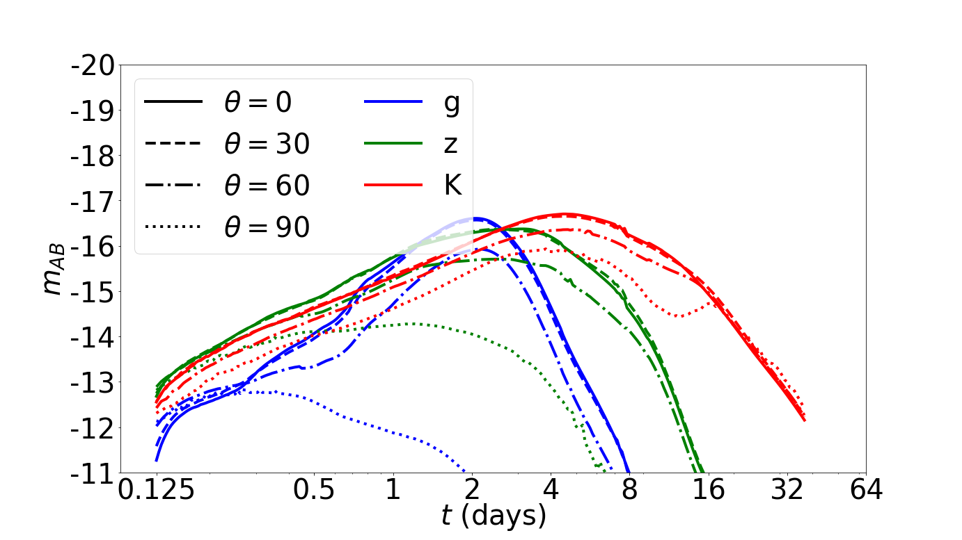
The ejecta model is based on a symmetrically-shaped ideal fluid expanding in vacuum described by the Euler equations of ideal hydrodynamics. The assumption of a radiation-dominated polytropic equation of state allows for an analytic representation of the ejected mass $M$ and average velocity $\bar{v}$ as a function of initial central density $\rho_{0}$, initial time $t_{0}$, and the velocity of the expansion front $v_{max}$ (Equations 11 and 12 in Wollaeger et al. (2018)). When combined with Monte Carlo-based radiative transfer and a specified elemental composition for the ejecta, the code produces time- and orientation-dependent spectra. Convolving these spectra with standard observational filters produces light curves such as the ones in Figures 1 and 4.

Figure 1: Bolometric luminosities of initial and adaptively placed simulations: The top panel shows the $\log_{10}$ bolometric luminosity in CGS units versus time in days for the simulations we initially used to train our grid. These simulations all extend out to roughly 8 days. The bottom panel shows the bolometric light curves for our adaptively placed simulations overlaid on top of the initial grid light curves. Most of these simulations extend past 32 days. Both panels exhibit significant diversity in behavior and timescale.

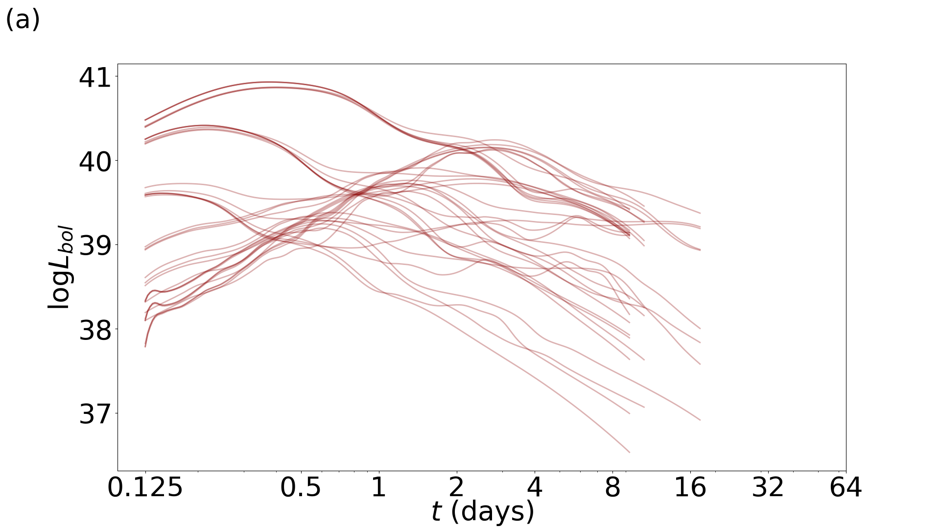
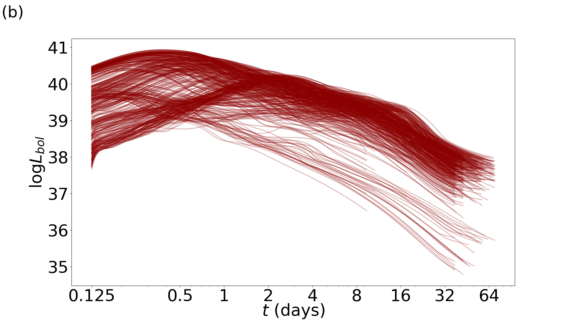
Real neutron star mergers have (at least) two mechanisms for ejecting material, denoted as dynamical and wind ejecta Radice et al. (2020). Due to the difference in formation mechanisms of dynamical and wind ejecta Metzger (2019), a multi-component approach is necessary for accurate modeling. Each of the two types of ejecta, dynamical and wind, is modeled by a separate component with a specified morphology, elemental composition, ejecta mass and ejecta velocity. The components are modeled together as one radiative outflow Wollaeger et al. (2018). The thermal decay energy is treated by mass-weighting between the components where they overlap. The end product represents a time-dependent spectral energy distribution contained in 54 angular bins, equally spaced in $\cos\theta$ from $1$ to $-1$. For the purposes of this study, the spectra are convolved with broadband filters to produce a series of broadband light curves. Specifically, we use the LSST $grizy$ filters for optical and near-infrared bands, 2MASS $JHK$ filters for longer wavelength near-infrared, and the mid-infrared $S$ filter for the Spitzer $4.5\;\mu$m band. For each band and emission direction, we estimate the AB magnitude for that filter, defined for a source at $10{\rm pc}$ in terms of the CGS energy flux $F_{\nu}$ per unit frequency via $m_{X,AB}=-2.5\log_{10}{\left\langle F_{\nu}\right\rangle}-48.6$. All observations used in this work are provided or are translated into this AB-magnitude system Bessell et al. (1998); Blanton and Roweis (2007); Hewett et al. (2006). Because our simulations tend toward reflection-symmetric behavior across the $z=0$ plane, we only consider the independent information contained in the upper half ($z>0$) of these angular bins. To reduce the acquisition cost of each simulation, we evolved each kilonova simulation in our initial grid out to $7.66$ days. To minimize data-handling and training cost, unless otherwise noted, we manipulate a subset of our simulation output based on a log-uniform grid. For the initial simulations, this log-uniform grid consists of 191 time points ranging from $1/8{}$ to $7.66$ days. For the remaining simulations, this grid is extended in log-time to cover their available duration, up to a maximum of 64 days. Because of several systematics associated with modeling emission at early times (e.g., in the ionization states of the medium and in the contribution from and interaction with any strong jet), we do not report on behavior prior to 3 hours post-merger. In this work, we use the orientation-averaged luminosity for simulation placement, but reconstruct the luminosity continuously in angle and time.

The original simulation hypercubes discussed in Wollaeger et al. (2018, 2021) consider multiple wind ejecta morphologies and compositions. To simplify the dimensionality of the problem, this work only considers simulations from the initial grid with a peanut-shaped morphology Korobkin et al. (2021) and lower $Y_{e}=0.27$ composition describing the wind ejecta. Table 1 summarizes the parameters for the 36 simulations in our four-dimensional hypercube and highlights variation in only ejected mass $M$ and average velocity $\bar{v}$ for each of the two components: the mass and velocity of the dynamical and wind ejecta, denoted henceforth as $M_{d},v_{d},M_{w},v_{w}$. Every simulation in our hypercube adopts the same morphologies for the dynamical and wind ejecta, respectively. This initial simulation hypercube thus consists of only 2 of the 3 velocities and 3 of the 5 masses explored in the companion study Wollaeger et al. (2021).

Ejecta	Morphology	$Y_{e}$	$M\textsubscript{ej}$	$\bar{v}$
			$M_{\odot}$	$c$
Dynamical	Torus	$0.04$	0.001, 0.01, 0.1	0.05, 0.3
Wind	Peanut	$0.27$	0.001, 0.01, 0.1	0.05, 0.3

Table 1: Kilonova simulation parameters: Within the framework of models explored in Wollaeger et al. (2021), parameters of the initial kilonova simulations used to initialize our adaptive learning process in this work. All simulations used in this work adopt a two-component model where the morphology and composition of each component is fixed.

As expected and discussed elsewhere Wollaeger et al. (2021), these simulations exhibit significant viewing-angle dependence on the relative speed of the components. The obscuration of the wind by the dynamical ejecta becomes less significant closer to the symmetry axis and the peanut morphology itself also produces orientation dependence. The two-component model shows “blanketing” of slow blue components by fast red components Kasen et al. (2015). Also expected and observed are qualitative trends versus the component masses and velocities: more wind ejecta mass increases the $g$-band luminosity along the symmetry axis.

Illustrating systematics of kilonova simulations

Before extensively discussing our ability to reproduce this specific family of simulations, we first comment on their systematic limitations. Our simulation archive explores only a limited range of initial conditions for the ejecta, with specific assumptions about the composition, morphology, and velocity profiles; with specific assumptions about nucleosynthetic heating; and with specific assumptions about (the absence of) additional power and components, such as a jet or a central source to provide additional power or light Nativi et al. (2021); Klion et al. (2021); Piro et al. (2018); Ai et al. (2018). Several previous studies have indicated that these and other aspects of kilonova simulations can noticably impact the outcome Wollaeger et al. (2018); Even et al. (2020); Wollaeger et al. (2019); Kawaguchi et al. (2021); Zhu et al. (2021); Korobkin et al. (2021); Perego et al. (2017). Where possible, we very briefly comment on how current and previous SuperNu simulations’ results change when making similar changes in assumptions.

Prior work with SuperNu has explored the impact of composition Even et al. (2020). However, recently, Kawaguchi et al 2020 Kawaguchi et al. (2021) (henceforth K20) demonstrated that Zr makes a substantial contribution to the final light curve. Figure 2 shows how our simulations depend on a similar change in composition, noting substantial change in the late-time optical light curves when we remove Zr.

As demonstrated by many previous studies using SuperNu, the morphology and velocity structure also has a notable impact on the post-day light curve behavior Wollaeger et al. (2018); Korobkin et al. (2021); Perego et al. (2017). Several other groups have demonstrated similar strong morphology and orientation dependence in their work Darbha and Kasen (2020); Kawaguchi et al. (2021); Breschi et al. (2021); Heinzel et al. (2021). For example, in their Figure 8, K20 demonstrate how the light curve changes when a specific polar component of the ejecta is removed.

Uncertain nuclear physics inputs also propagate into notable uncertainties about the expected light curve; see, e.g., Zhu et al. (2021); Barnes et al. (2021). Even for the same morphology and amount of ejecta, nuclear physics uncertainties can modify the effective heating rate, particularly for material with low $Y_{e}$ which has the greatest prospect for producing r-process elements.

Given limited exploration of possible kilonova initial conditions and physics, we can only at present quantify the uncertainties of the type listed above. In future work, we will employ our parameterized models to assess the impact of these uncertainties on inferences about kilonova parameters. Future work could require kilonova models which include EOS parameters to enable joint inference which also simultaneously constrains the equation of state.

Figure 2: Impact of removing Zirconium: Solid and dashed lines show simulations with otherwise identical assumptions about composition, morphology, and velocity structure, differing only by the presence (solid) and elimination (dashed) of Zr. The selected simulation parameters, $M_{d}=0.01M_{\odot}$, $v_{d}=0.3c$, $M_{w}=0.01M_{\odot}$, and $v_{w}=0.15c$, are our closest-matching representation of the simulation parameters considered during the Zr-omitting study in Kawaguchi et al. (2021).

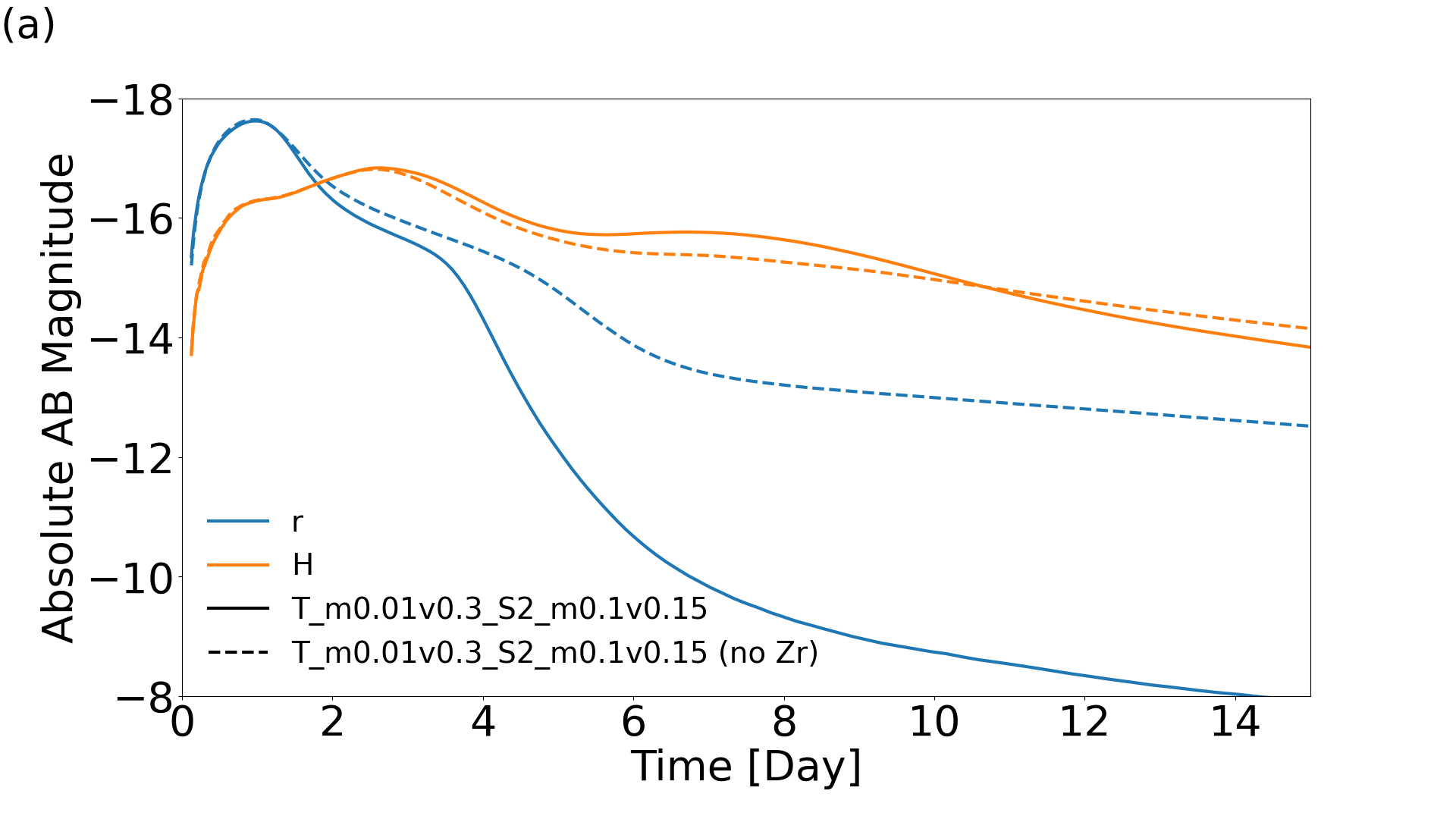
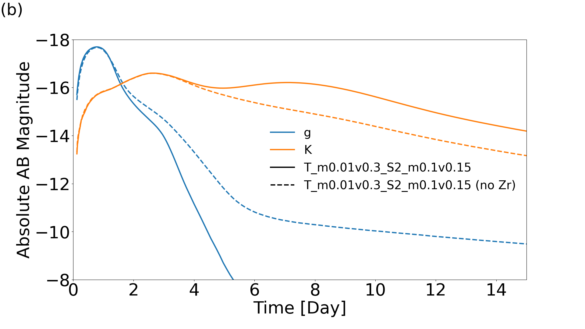
As discussed elsewhere Wollaeger et al. (2021), at late times some light curves show a modest deficit of blue light ($g$-band) relative to observations of GW170817 (unless the dynamical ejecta mass is large). Notably, our $g$-band light curves fall off significantly more rapidly after their peak in all viewing directions and for most parameters considered here. Previous work with other morphologies also recovers similar falloff in these bands, see e.g. Tanvir et al. (2017), though additional components could conceivably contribute. Similar $g$-band behavior has been seen in other detailed kilonova simulations; see, e.g, Figure 12 in Kawaguchi et al. (2020). As noted above, this behavior depends on the assumed composition, notably Zr.

II.2 Interpolation Methodology

In this work, we principally interpolate using Gaussian process (GP) regression. In GP regression, given training data pairs $(x_{a},y_{a})$, the estimated function $\hat{y}(x)$ and its variance $s(x)^{2}$ are approximated by

$$\hat{y}(x) =\sum_{a,a^{\prime}}k(x,x_{a})K^{-1}_{aa^{\prime}}y_{a^{\prime}}$$ (1a)

$$s(x)^{2} =k(x,x)-k(x,x_{a})K^{-1}_{aa^{\prime}}k(x_{a^{\prime}},x)$$ (1b)

where the matrix $K_{aa^{\prime}}=k(x_{a},x_{a^{\prime}})$ and where the function $k(x,x^{\prime})$ is called the kernel of the Gaussian process. In this work, unless otherwise noted, we used a squared-exponential kernel and a white noise (diagonal) kernel

$$k(x,x^{\prime})=\sigma_{o}^{2}e^{-(x-x^{\prime})Q(x-x^{\prime})/2}+\sigma_{n}^{2}\delta_{x,x^{\prime}}$$ (2)

where $Q$ is a diagonal matrix of possible length scales and $\sigma_{0},\sigma_{n}$ are hyperparameters that characterize the amount of noise allowed in the problem. The other interpolation method considered in this work was random forest (RF) regression Breiman (2001). Unlike the GP, the RF output had no error quantification and was used primarily as a consistency check on the Gaussian process prediction. Unless otherwise noted, we performed all GP and RF regression with scikit-learn Pedregosa et al. (2011).

Because of the substantial dynamic range of our many outputs, we interpolate the $\log_{10}$ luminosity (for placement) or AB magnitudes (for all other results). Unless otherwise noted, we quantify the performance of our interpolation with the RMS difference between our prediction and the true value

$$\ell^{2}=\frac{1}{n}\sum_{j=1}^{n}(y_{j}-\log_{10}(L_{\text{bol}})_{j})^{2},$$ (3)

[This expression overweights the importance of large errors when the source is not detectable at late times; see Appendix A].

We employ GP interpolation in two standard use cases. In the first case, used for our exported production results, we interpolate the AB magnitude $m_{\alpha}(t_{*}|\Lambda)$ at some fixed reference time $t_{*}$ and band $\alpha$ versus our four simulation hyperparameters (and, in the end, also across the extrinsic parameters of angle and wavelength) contained in $\Lambda$. In this case, the prediction $y(x_{a})$ has a single scalar value at each point; the $x_{a}$ refer to model hyperparameters; and the interpolation provides us with a scalar function of four or more variables. GP regression [Eq. (1)] provides an error estimate for $m_{\alpha}$ at this specific time $t_{*}$, which in general will depend on time.

In the second case, used for simulation placement, we interpolate the log bolometric luminosity light curve $\log_{10}L_{bol}(t|\Lambda)$ versus all time. [In terms of each simulation’s spectrum, the bolometric luminosity is $L_{bol}=4\pi R^{2}\int_{0}^{\infty}F_{\nu}d\nu$ where R = 10 pc.] In this case, the prediction $\vec{y}(x_{a})$ is vector-valued at each point; the $x_{a}$ refer to model hyperparameters; and the interpolation provides us with a vector-valued function of four or more variables. For simplicity and given our use case, we reduce our error estimate to a single overall value for the entire light curve, reflecting the overall uncertainty in $\vec{y}(x_{a})$.

II.3 Active Learning Scheme

Gaussian processes have long been used for active learning because they provide an error estimate: follow-up simulations can be targeted in regions with the largest expected error (and thus improvement) Murphy (2012). We follow this approach in our active learning scheme; see Solomon and Zacks (1970); Krause and Guestrin (2007); Cohn et al. (1996); Gal et al. (2017); MacKay (1992); Srinivas et al. (2012); Mockus et al. (1978); Wu and Frazier (2018) for a broader discussion of active learning methods and their tradeoffs. To reduce the data volume needed for targeting followup simulations, we used vector-valued interpolation as described above, applied to orientation-averaged outputs of our simulations. This approach has the substantial advantage of providing a single error estimate per light curve (both in training and off-sample), which we can immediately use as an objective function in a minimization algorithm.

We pursued an active learning simulation placement approach in order to maximally explore the parameter space and reduce the amount of redundant information obtained from each new simulation. The subset of 36 light curves discussed in Section II.1 was used as the initial training set. Thousands of parameter combinations were subsequently drawn from uniform distributions with maxima and minima matching those of the varied parameters in Table 1. Each of these parameter combinations was evaluated by an interpolator to produce an initial light-curve prediction as well as an error on the entire light-curve output. The prediction with the largest error across all the tested parameter combinations was selected as the next placed simulation.

Figure 3: Impact of adaptive placement on interpolation: Example of interpolation output at a point with large predicted fitting error, both before and after placing the simulation. In both panels, the solid black curve shows the true simulated bolometric light curve versus time. The red band shows the GP-predicted one-sigma error bar about the expected value. Top panel: Predictions from our RF and GP interpolations versus time. The large error and low practical utility of the GP fit is apparent. Bottom panel: After including this simulation in the training set, the revised RF and GP predictions much more closely conform with this specific simulation as expected.

II.4 Prediction Improvement and Interpolation Results

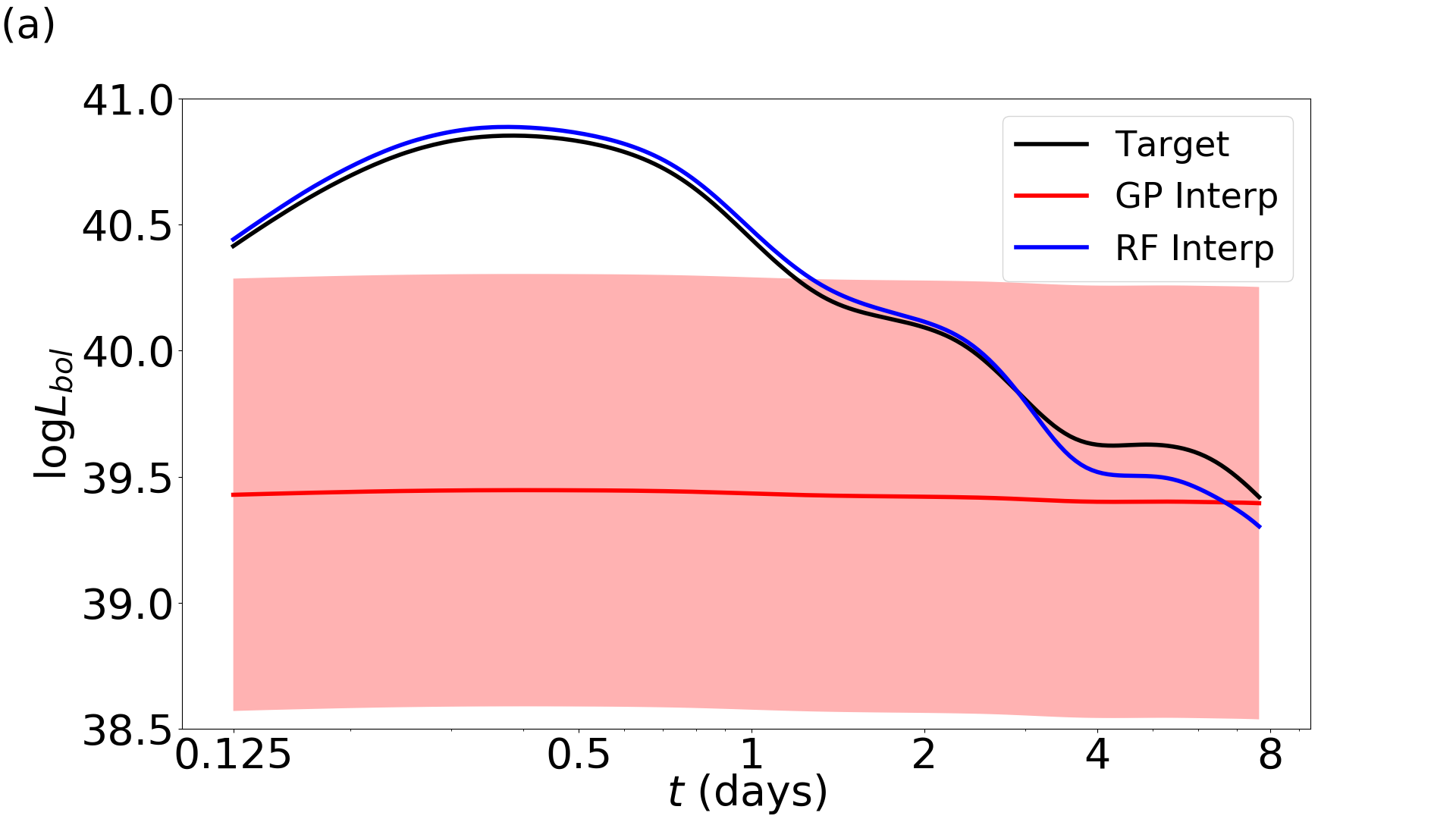
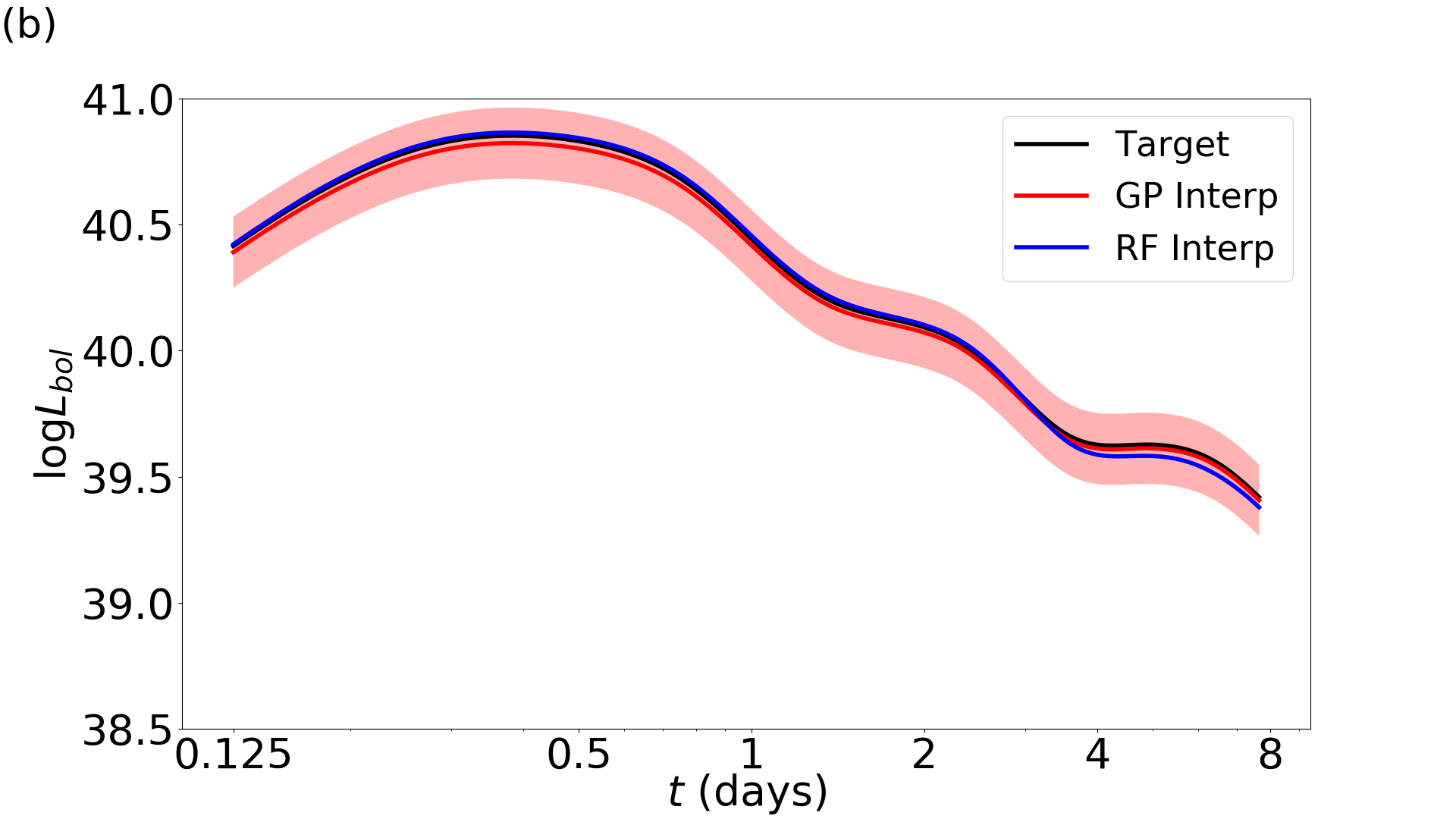
We verified our active learning strategy for simulation placement by randomly sampling combinations of parameters and creating two light curve predictions based on those parameters. The first prediction was trained solely on our initial grid of simulations from Section II.1, while the second prediction was trained on the same initial grid, but with an added simulation output characterized by the aforementioned random combination of parameters. Figure 3 shows these before- and after-inclusion predictions which show that, as expected, the GP interpolation capability is improved. This pair of figures anecdotally illustrates the degree to which new training data improves our surrogate light curve models.

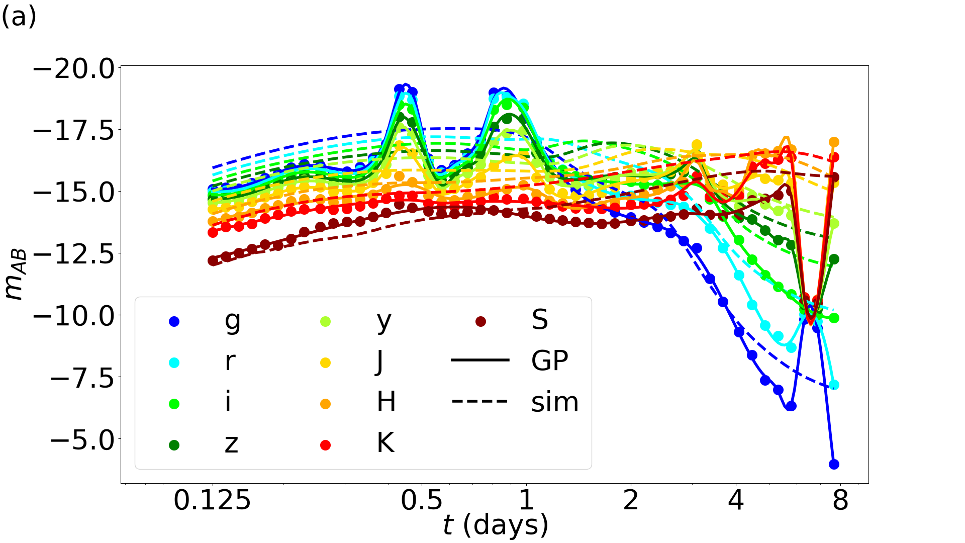
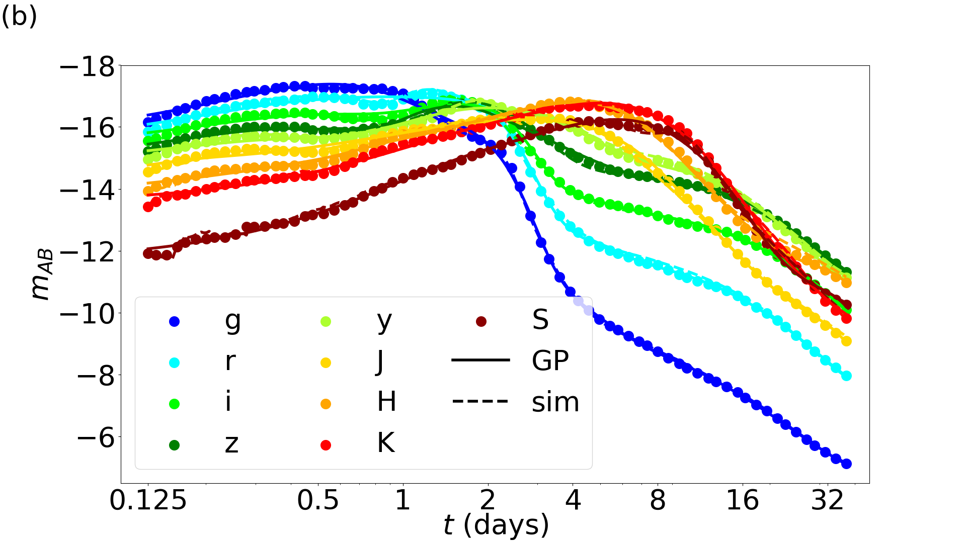
With over 400 placed simulations since the start of the active learning process, the training library is built up enough to allow for physically meaningful interpolation of off-sample events. The performance of our adaptive learning is best illustrated with our production-quality interpolation scheme, illustrated in Figure 4 and described in the next section.

Despite producing many follow-up simulations, we achieve success with a very sparse coverage of our parameter space. To illustrate the sparsity of our parameter space coverage, and how slowly our added simulations increase coverage, we evaluated the median “inter-simulation” distance, using a simple Euclidean ($L^{2}$) norm over $\log_{10}L_{bol}(t_{k})$ for several reference times $t_{k}$. As expected given the high apparent dimension of our output, this median distance changes very slowly with $n$, owing to the large effective dimension of the output light curves. The median distance is also larger than the residual error in our fit, as reported below. The success of our interpolation relies not on an overwhelmingly large training sample, but on the smoothness and predictability of our physics-based light curves.

III Light curve interpolation

III.1 Stitched fixed-time interpolation

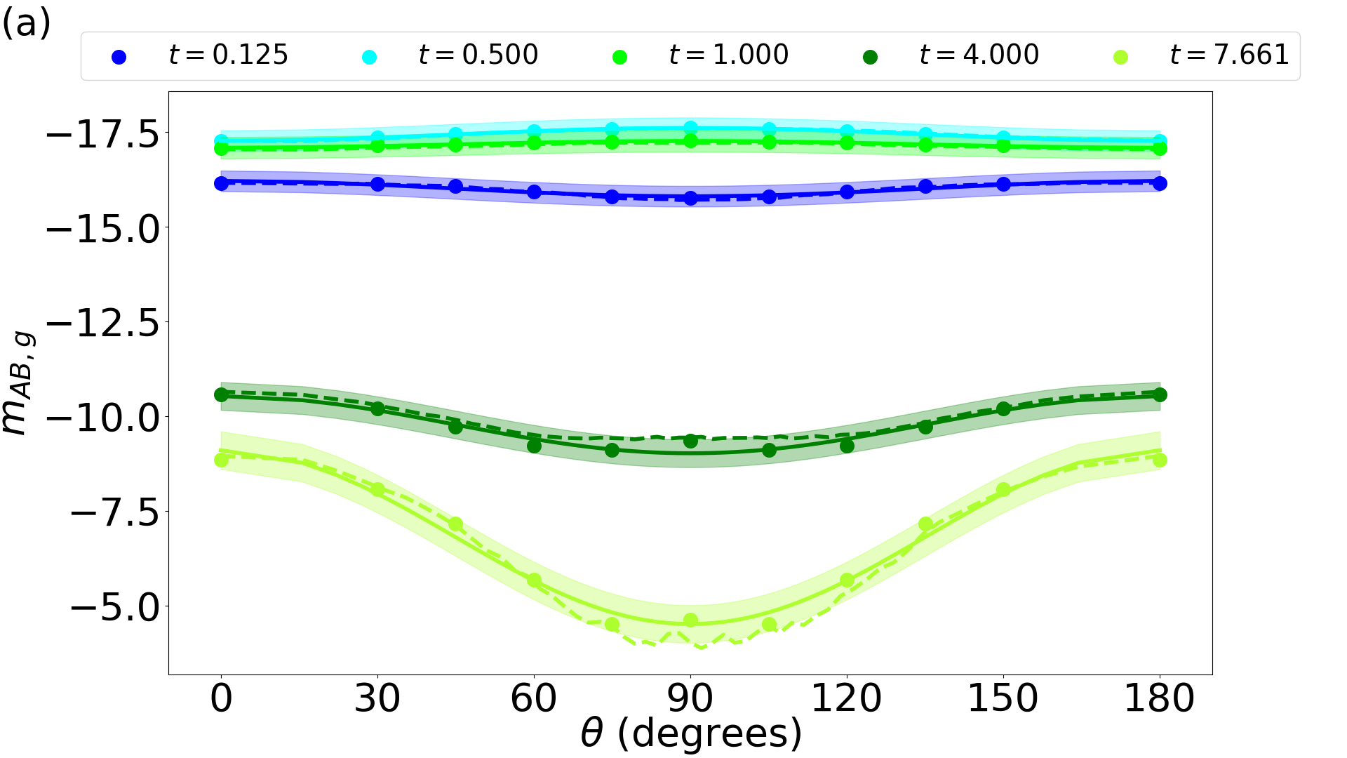
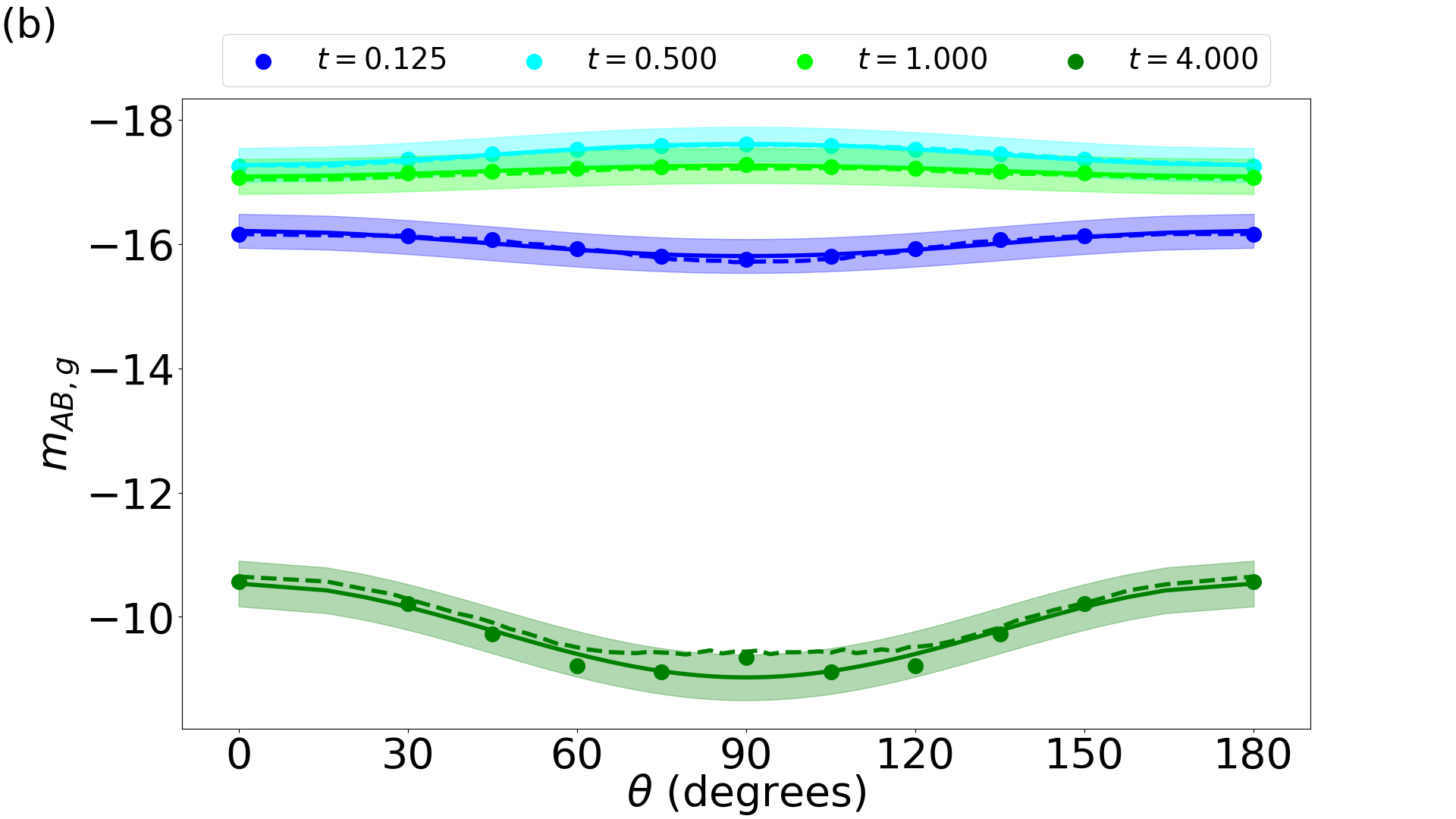
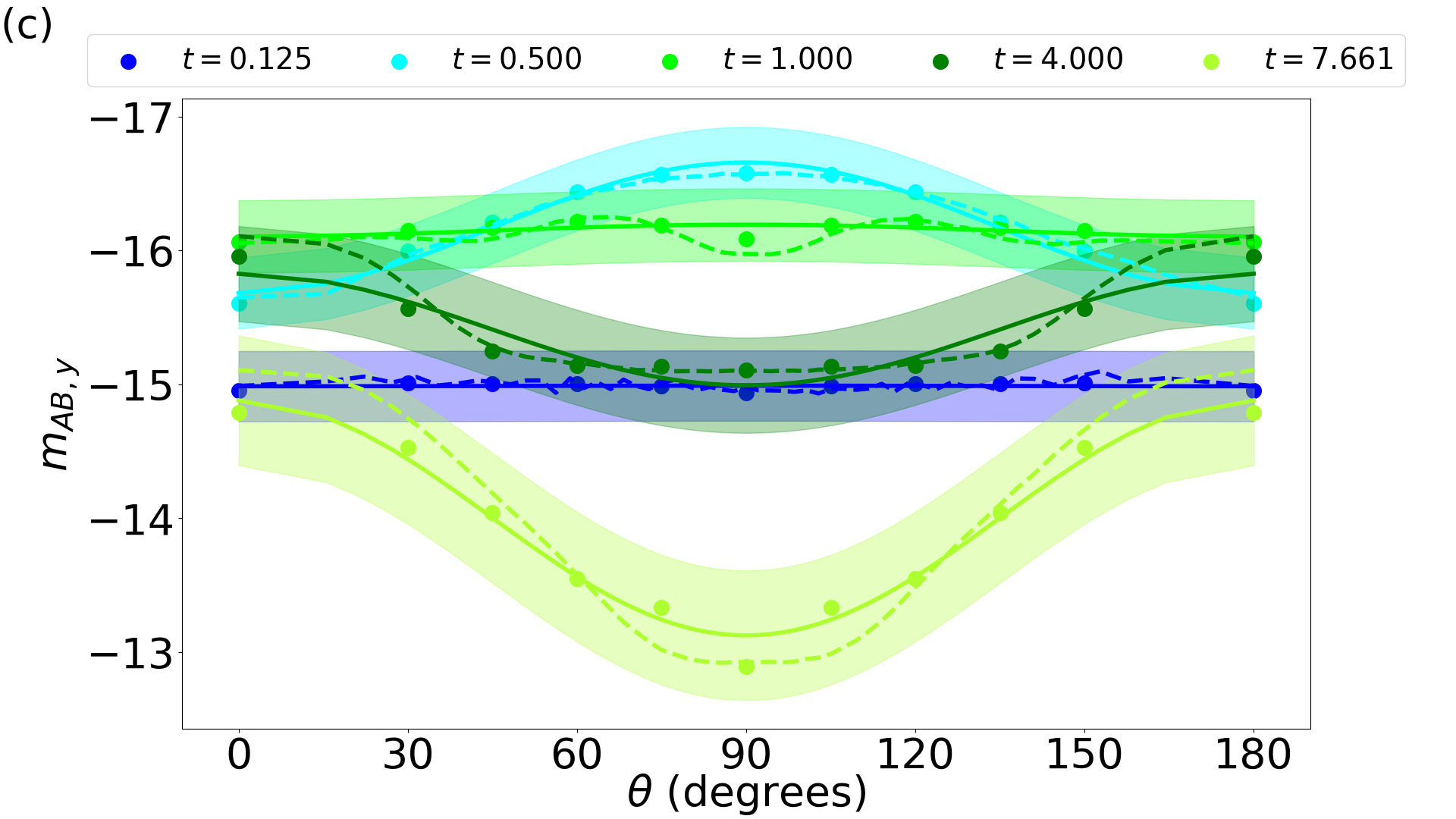
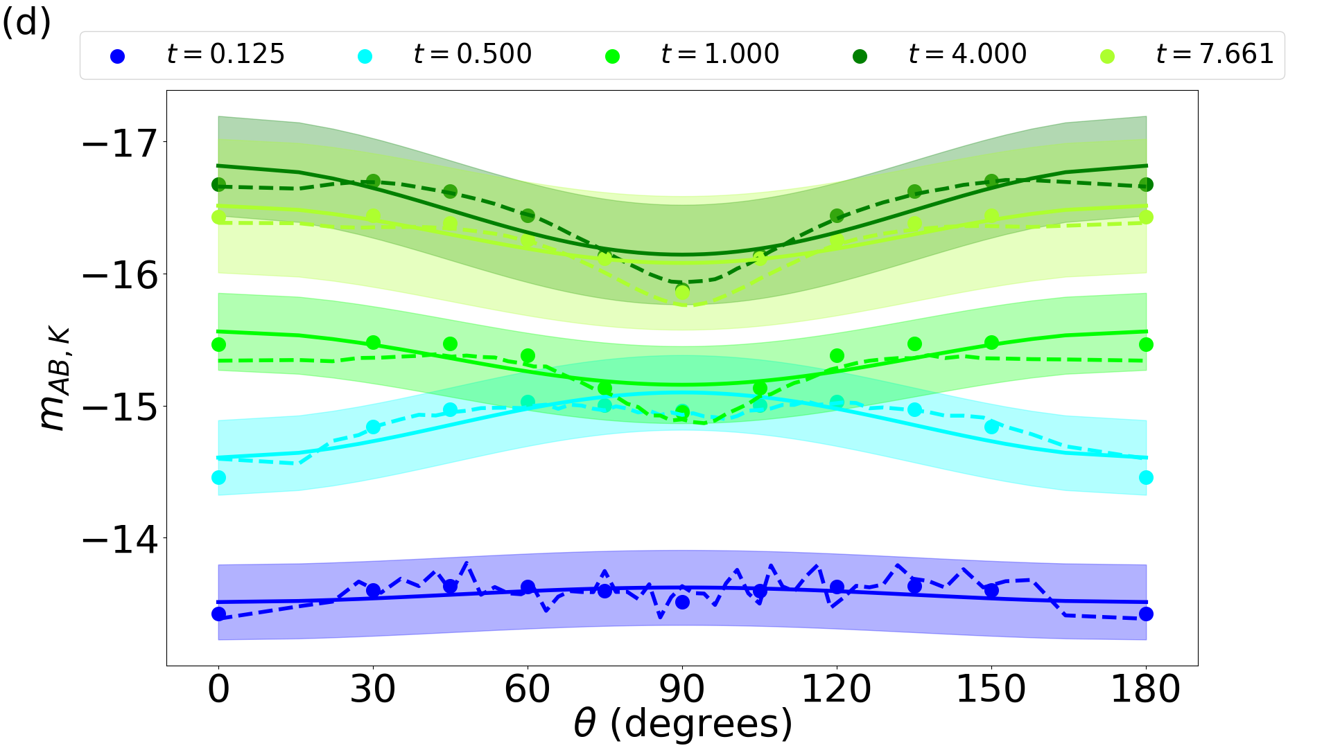
To efficiently interpolate across the whole model space, we follow a strategy illustrated in Figure 1 of Field et al. (2014): we pick several fiducial reference times $t_{q}$ (and angles); use GP interpolation to produce an estimate $m_{\alpha}(t_{q}|\Lambda)$ versus $\Lambda$; interpolate in time to construct a continuous light curve at the model hyperparameters $\Lambda$ at each reference angle; and then interpolate in angle to construct a light curve for an arbitrary orientation. For an error estimate, we stitch together the error estimates in each band to produce a continuous function of time. Figure 4 shows the output of our interpolation (smooth lines), compared to a validation simulation at the same parameters (dashed lines). Our predictions generally agree, though less so for the shortest wavelengths at the latest times. Subsequent figures also illustrate the typical GP error estimate, which is usually $O(0.1)$ in $\log_{10}L$ for most bands and times considered.

Figure 4: Off-sample interpolation with original and refined grid: Example of an interpolated stitched fixed-time prediction compared to a simulation output created from the same corresponding input parameters. The top panel shows our estimate based on the initial $36$ simulations; the bottom panel shows the result after adaptive learning. Different colors denote different filter bands, described in the legend. The dashed lines show full simulation output for each band. The colored points show our interpolated bolometric magnitude predictions at the $191$ evaluation times. The solid lines show our final interpolated light curves, interpolating between the points shown. The largest error in this example occurs for the $g$-band at late times. The simulated parameters and viewing angle for this configuration are $M_{d}=0.097050M_{\odot}$, $M_{w}=0.083748M_{\odot}$, $v_{d}=0.197642c$ and $v_{w}=0.297978c$, viewed on axis ($\theta=0$). The exaggerated modulations in the top panel’s solid lines and dotted curves illustrate interpolation failures, arising from adopting an initially insufficient training set.

III.2 Trends identified with interpolated light curves

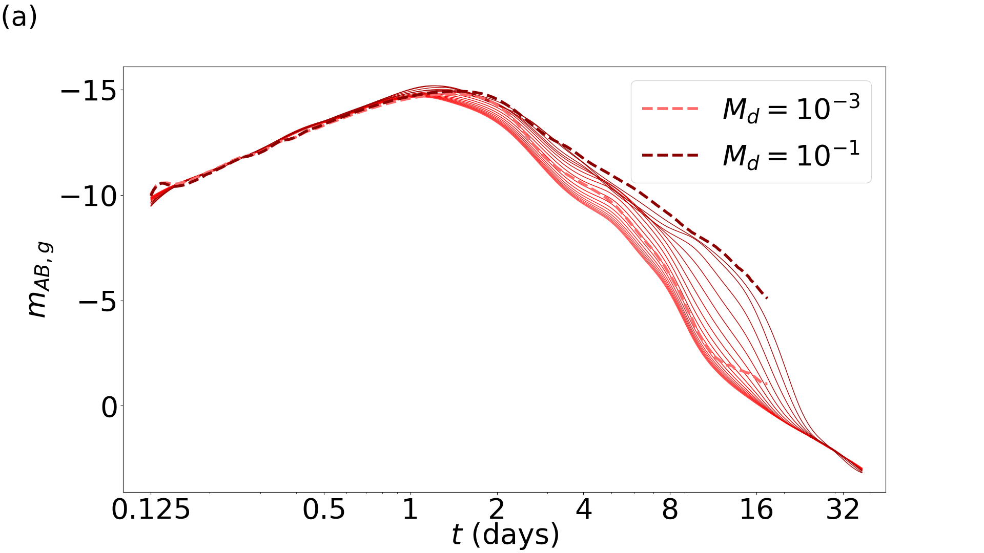
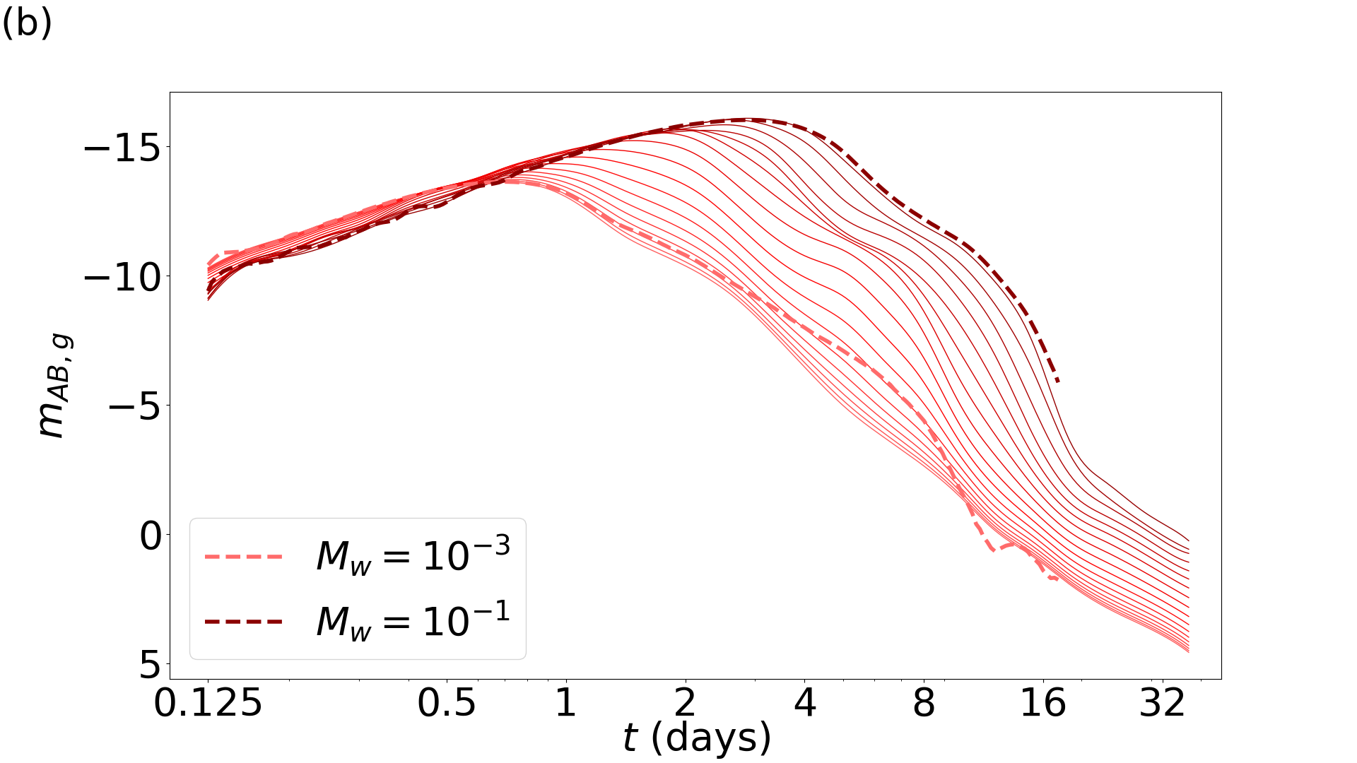
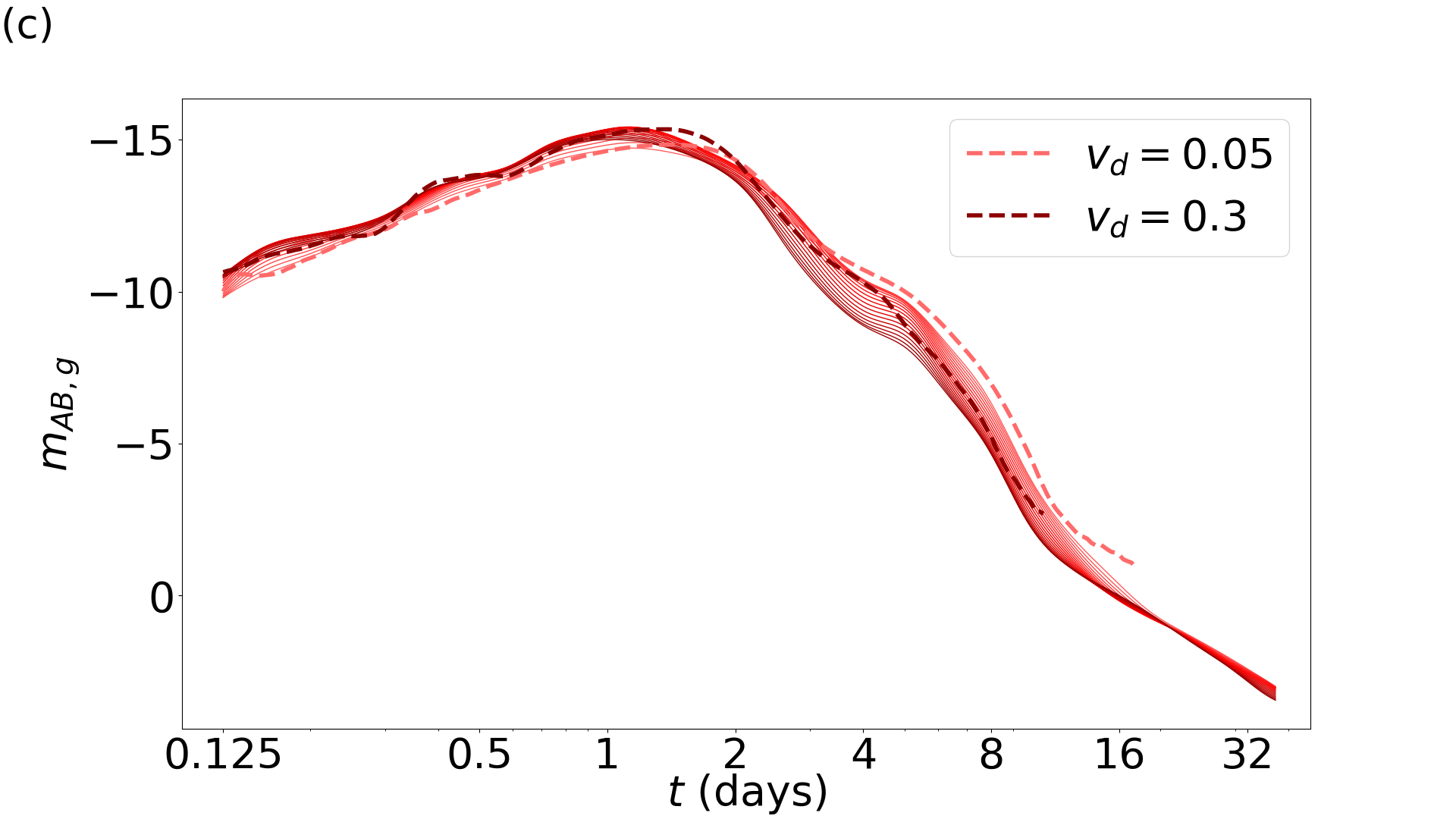
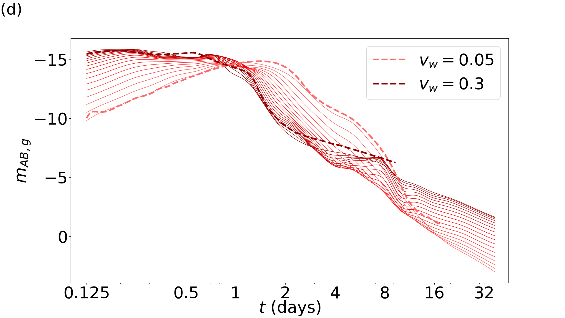
In Figure 5 we show the results of our fit evaluated at a fixed viewing angle ($\theta=0$), varying one parameter at a time continuously, relative to a fiducial configuration with $M_{d}=M_{w}=0.01M_{\odot}$, $v_{w}/c=v_{d}/c=0.05$. The fixed value for the ejected mass of $M=0.01M_{\odot}$ was chosen as the middle ground of the initial grid’s sampled mass space, which does not introduce any biases toward lighter or heavier masses. Since no similar central value was initially available for the velocity parameters, the lower value was selected in the case of both components. The slower velocity resulted in the ejecta not dissipating as quickly and allowed for more variation in the light curves as the non-static parameter was varied. For this viewing angle, changes in the amount and velocity of the dynamical ejecta have relatively modest effect, in large part because that ejecta is concentrated in the equatorial plane. By contrast, changes in the mostly polar wind ejecta has a much more substantial impact on the polar light curve ($\theta=0$). Specifically, increasing the amount of wind ejecta brightens and broadens the light curve, as expected from classic analytic arguments pertaining to how much material the light must diffuse through Arnett (1980, 1982); Chatzopoulos et al. (2012); Metzger (2019). Similarly, increasing the velocity of wind ejecta causes the peak to occur at earlier times (diffusion is easier) and be brighter.

Figure 5: Interpolated and simulated $g$-band light curves: In this figure, we generate $\log L_{g}(t|\Lambda)$ for a one-parameter family of simulations $\Lambda$ where either one of the $M$ parameters vary from $0.001M_{\odot}$ to $0.1M_{\odot}$ or one of the $v$ parameters vary from $0.05c$ to $0.3c$, and the viewing angle is $\theta=0$. The remaining model parameters are fixed to $(M/M_{\odot},v/$c$)=(0.01,0.05)$. Contours in $M$ are uniform in $\log M$, while those for $v$ are linearly uniform. For comparison, the heavy dashed lines show the initial training simulation results for the two parameter endpoints. The $g$-band light curve has the largest dynamic range and is the most sensitive to interpolation errors; notably, the interpolation does not always conform tightly to the underlying simulation data at late times.

III.3 Interpolation in viewing angle

All of the interpolated light curves discussed thus far have been trained at some fixed viewing angle. In Figure 6, we explore the interpolation of several families of models, each of which was trained using simulation data at a different viewing angle. The symmetry of the ejecta across the orbital plane allows for the assumption that any angular variation between $0$ and $\pi/2$ can simply be mirrored across the symmetry axis.

Figure 6 indicates that the first day post-merger does not introduce much angular variation and, as such, is quite well predicted even when interpolating across only 11 angles. After 1 day, the luminosity across different angles begins to change considerably as the peanut-shaped wind ejecta becomes more dominant. Particularly at late times, there is a strong angular variability which manifests near the orbital plane, most strongly apparent in the blue ($g$) and near infrared ($K$) bands. In the blue bands, the angular variation reflects lanthanide curtaining; in the red bands, the angular variation reflects red emission from the late-peaking red dynamical ejecta. [At the latest times and faintest luminosities along the equatorial plane, numerical uncertainty in our Monte Carlo simulations are apparent in the light-curve results.] In all panels, the solid band denotes an estimated error bar from our GP fit in time, extended in angle.

Figure 6: Interpolation of $g$-, $y$-, and $K$-band luminosity at different viewing angles: This figure compares the $g$-, $y$-, and $K$-band luminosity at select times as a function of viewing angle. The solid points represent fixed angles at which the different families of models were trained. The solid lines connecting the points indicate the interpolated prediction of the angular variation at some given time in the light curve. The dashed lines represent the simulation data and show the true angular variation. The shaded regions denote the $1\sigma$ error estimate derived from our Gaussian process fit versus time, extended in angle.

III.4 Predictive Accuracy versus time, angle grid sizes

To better understand the systematic limitations and computational inefficiencies introduced by our stitched-time interpolation grid, we investigated the accuracy of our fits when only using a subset of the time or angular grid.

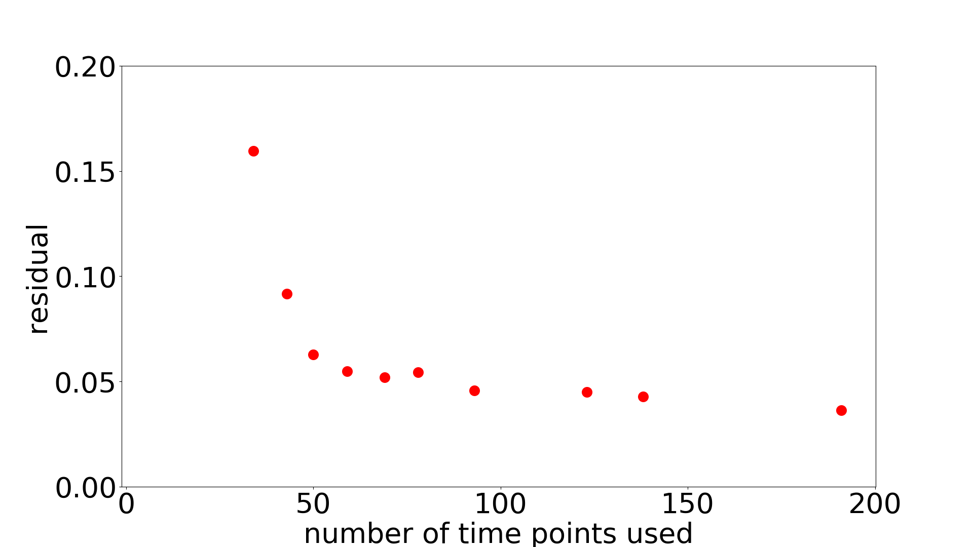
First, we consider a simple analysis of loss of predictive accuracy as the number of GP interpolators used to make a surrogate light curve is decreased. We denote $t\in T$ as the subset of times represented by the GP interpolators used to make a prediction, $T$ as the total available number of time points, and thus interpolators, which can be used to make a light curve, and $\bar{t}$ as all the other times in $T$ which are not represented by $t$ such that $t\cap\bar{t}=0$ and $t\cup\bar{t}=T$.

Thus, when using any number of interpolators at times $t\in T$ which is less than the total number of possible time points $T$, we first generate predictions $y(t)$ with the chosen subset of interpolators. These predictions $y(t)$, along with the times $t$ at which the predictions were made, are then used as inputs for SciPy’s UnivariateSpline method from which the remainder of the light curve $z(t)=f({t},y(t))$ is constructed, where in this last case the function can be evaluated $\forall t\in T$.

Figure 8 shows how the average residual between on-sample light curve predictions and the respective simulation data changes as a function of the number of time points used as the base for constructing the time-interpolated light curve. For the current scheme, we can remove up to roughly 75% of the initial set of time points without substantially diminishing our overall accuracy. Future work will explore smarter selection of representative time points in an effort to further reduce the number of interpolators which can be removed without significant loss of accuracy.

Figure 7: Light curve versus time for selected angles and bands: Comparison to Figure 7 of Kawaguchi et al. (2020) indicating angular dependence of light-curve predictions across the $g$-, $z$- and $K$-bands.

Figure 8: Average residual as a function of number of considered time points: A plot of the average residuals between on-sample time-interpolated light curves and the respective simulation data as a function of how many time points are used to generate the light curves. In each case, we drew the respective number of samples from a log-uniform distribution between the start and end time of our light curves.

IV Parameter inference of radioactively-powered kilonovae

In this section, we describe and demonstrate the algorithm we use to infer kilonova parameters given observations, using the interpolated light-curve model above. Unless otherwise noted, for simplicity all calculations in this section assume the kilonova event time and distance are known parameters. We likewise assume observational errors are understood and well characterized by independent Gaussian magnitude errors in each observation, and that our model families include the underlying properties of the source (i.e., we neglect systematic modeling errors due to the parameters held constant in our simulation grid: morphology, initial composition, et cetera).

IV.1 Framework and validation

As in many previous applications of Bayesian inference to infer parameters of kilonovae Heinzel et al. (2021); Coughlin et al. (2018, 2019); Villar et al. (2017); Smartt et al. (2017), we seek to compare the observed magnitudes $x_{i}$ at evaluation points $i$ (denoting a combination of band and time) to a continuous model that makes predictions $m(i|{\bm{\theta}})$ [henceforth denoted by $m_{i}({\bm{\theta}})$ for brevity] which depend on some model parameters $\theta$. Bayes theorem expresses the posterior probability $p({\bm{\theta}})$ in terms of a prior probability $p_{\rm prior}({\bm{\theta}})$ for the model parameters $\bm{\theta}$ and a likelihood ${\cal L}(\theta)$ of all observations, given the model parameters, as

$$p({\bm{\theta}})=\frac{{\cal L}({\bm{\theta}})p_{\rm prior}({\bm{\theta}})}{\int d{\bm{\theta}}{\cal L}({\bm{\theta}})p_{\rm prior}({\bm{\theta}})}$$ (4)

Unless otherwise noted, for simplicity we assume the source sky location, distance, and merger time are known. We adopt a uniform prior on the ejecta velocity $v/c\in[0.05,0.3]$ and a log uniform prior on the ejecta masses $m/M_{\odot}\in[10^{-3},0.1]$. We assume the observations have Gaussian-distributed magnitude errors with presumed known observational (statistical) uncertainties $\sigma_{i}$, convolved with some additional unknown systematic uncertainty $\sigma$, so that

$$\ln\mathcal{L}(\bm{\theta})=-0.5\sum_{i=1}^{n}\left[\frac{(x_{i}-m_{i}(\bm{\theta}))^{2}}{\sigma_{i}^{2}+\sigma^{2}}+\ln(2\pi(\sigma_{i}^{2}+\sigma^{2}))\right]$$ (5)

where the sum is taken over every data point in every band used in the analysis. In tests, we treat $\sigma$ as an uncertain model parameter, de facto allowing for additional systematic observational uncertainty (or for some systematic theoretical uncertainty). For our GP surrogate models, we set $\sigma$ to the estimated GP model error.

Unlike prior work, we eschew Markov-chain Monte Carlo, instead constructing the posterior distribution by direct Monte Carlo integration as in Pankow et al. (2015); Lange et al. (2018). To efficiently capture correlations, we employ a custom adaptive Monte Carlo integrator; see Champion et al. (2021) for implementation details. In Appendix A, we describe several tests we performed to validate this inference technique using synthetic kilonova data drawn from a previously published semianalytic kilonova model. Our tests include recovering the parameters of a hundred synthetic kilonova sources. In future work, we will demonstrate how our parameter inference method can be incorporated efficiently and simultaneously with gravitational wave (GW) parameter inference with the rapid iterative fitting (RIFT) parameter estimation pipeline Lange et al. (2018).

IV.2 Inference with surrogate kilonova model

Figure 9: Synthetic source recovery with surrogate model: Recovery of a parameters of a known two-component surrogate kilonova model, using inference based on our interpolated model. Solid black curves show results adopting a strong angular prior motivated by radio observations of GW170817. Top panel: Synthetic light cuve data in several bands. Bottom panel: Inferred distribution of the four model parameters, and viewing angle. The blue cross denotes the injected values. Red contours show results without adopting a prior on observing angle; black contours show results inferred when adopting a prior on viewing angle consistent with observations of GW170817.

Figure 10: Simulation parameter recovery with surrogate model: Recovery of a parameters of a known two-component kilonova simulation, using inference based on our interpolated model. The parameters corresponding to the relevant simulation are $M_{d}=0.052780M_{\odot}$, $v_{d}=0.164316c$, $M_{w}=0.026494M_{\odot}$, and $v_{w}=0.174017c$. Top panel: Synthetic light curve data in several bands. Bottom panel: Inferred distribution of the four model parameters.

Figure 11: Simulation parameter recovery with analytic model: Recovery of a parameters of a known two-component kilonova simulation, using inference based on the simplified analytic model described in the appendix. The analytic model cannot fit our simulation data. While only a one-component fit is shown, similar results arise when employing multiple components. The parameters corresponding to the relevant simulation are $M_{d}=0.01M_{\odot}$, $v_{d}=0.3c$, $M_{w}=0.01M_{\odot}$, and $v_{w}=0.3c$. Top panel: Synthetic light curve data in several bands, including error bars on both the synthetic data and posterior light curve predictions. The analytic model cannot fit our simulated data well. Bottom panel: Inferred distribution of the four model parameters. The blue cross denotes the injected values.

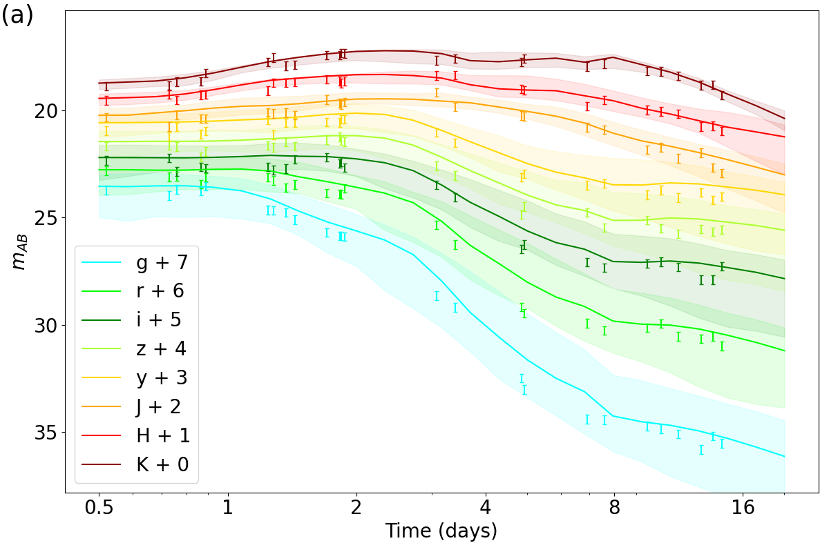
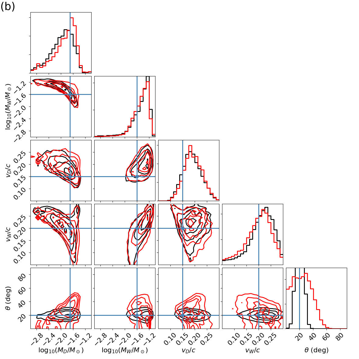
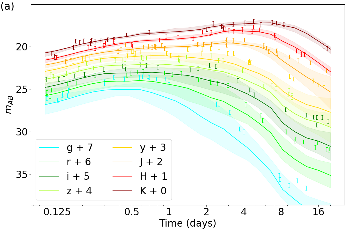
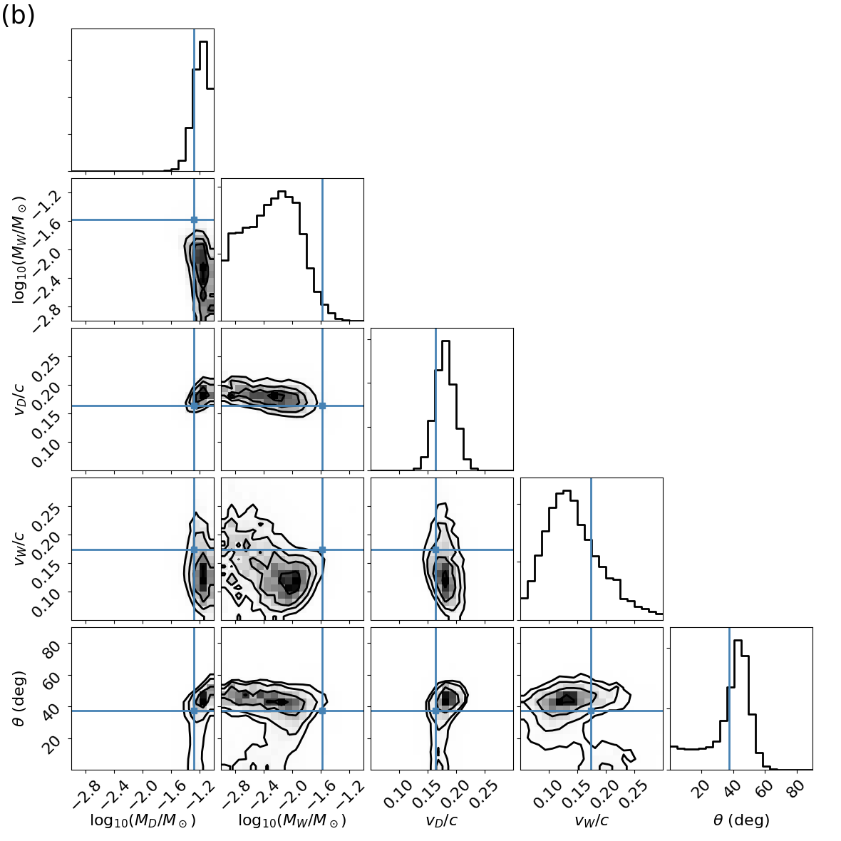
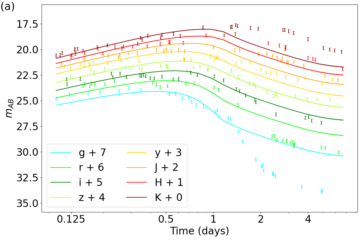
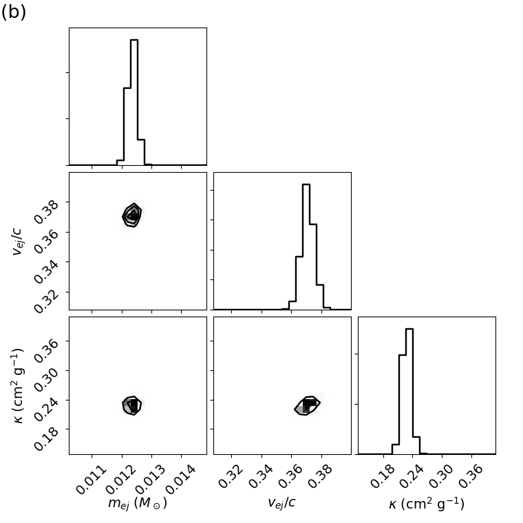
Figure 9 demonstrates parameter inference using our surrogate light curves, for a synthetic source generated using our own model. As expected, we can recover a known source, including constraining the viewing angle $\theta$. Figure 10 performs a similar test, but now using a specific simulation, without interpolation. As expected given our adopted systematic error, we recover the simulation parameters. Finally, Figure 11 repeats the test above, using the semianalytic model described in the appendix. This comparison emphatically demonstrates large systematic differences between this semianalytic model and our detailed simulations.

IV.3 Example: GW170817

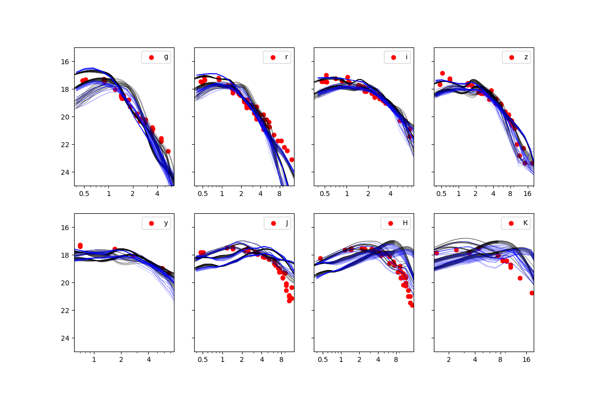
SuperNu-based kilonova models have already been successfully used to interpret GW170817, though as noted previously these models have a rapid falloff in the late-time optical magnitudes that is not present in the observations; see Tanvir et al. (2017). Because of the close proximity of GW170817, only distance modulus (but not redshift) corrections are needed to translate our predictions to apparent magnitudes which can be directly compared to electromagnetic observations. Observational results are taken from (Villar et al., 2017)’s compilation of photometry reported in Arcavi et al. (2017); Tanvir et al. (2017); Troja et al. (2017); Cowperthwaite et al. (2017); Drout et al. (2017); Smartt et al. (2017); Valenti et al. (2017); Pian et al. (2017); Kasliwal et al. (2017); Shappee et al. (2017); Utsumi et al. (2017). Figure 12 shows the results of directly comparing our extended simulation archive directly to observations of GW170817, selecting for simulations (parameters and angles) with the highest overall likelihood. The solid black curves in these figures show the 50 highest-likelihood configurations, where the likelihood requires simultaneously reproducing all observed bands. Except for reddest three bands (JHK), many simulations compare extremely favorably to the observations. The parameters of these simulations, however, do not represent the optimal parameters of this model family: because our placement algorithm minimizes interpolation error, the selected points preferentially occur at the edges of our domain. Finally, for the reddest band ($K$), our fits exhibit notable systematic uncertainty relative to the underlying simulation grid.

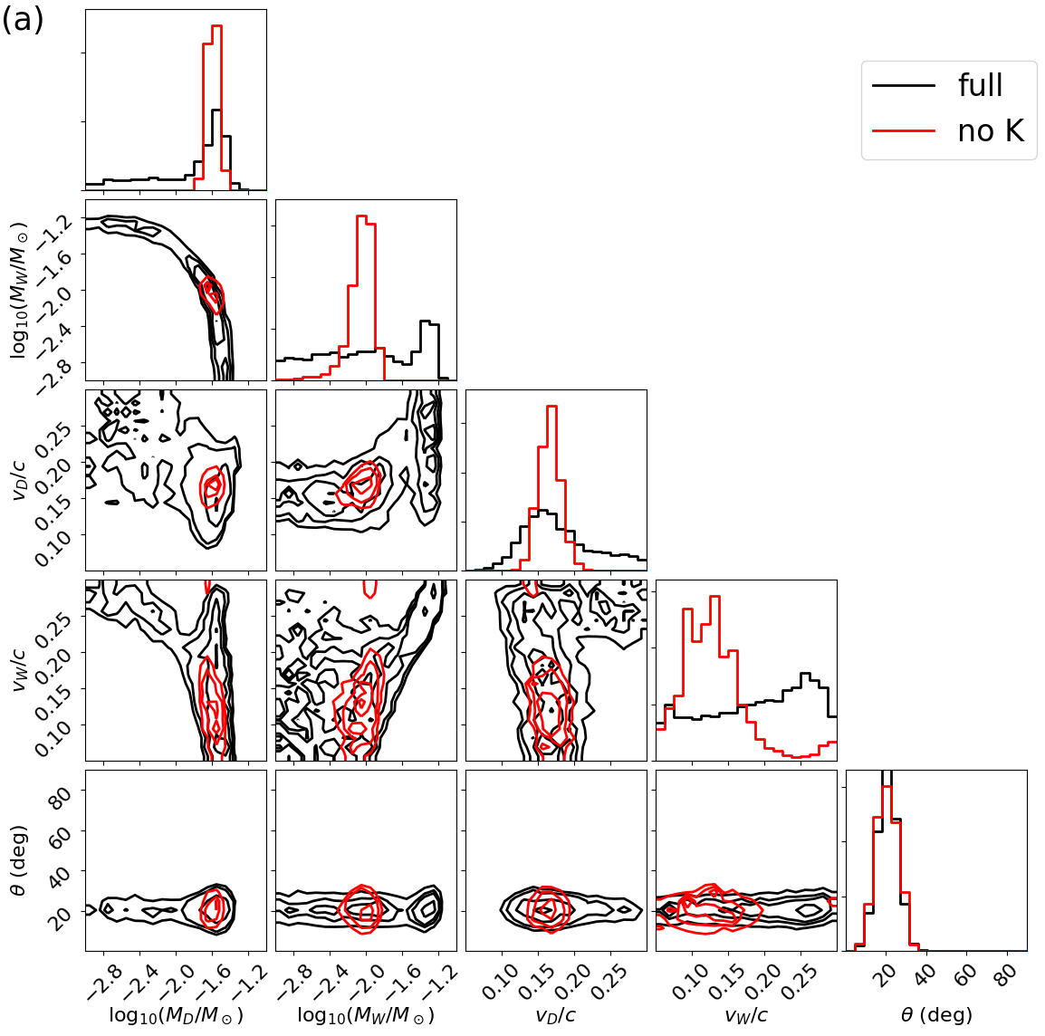
We have performed parametric inference on GW170817 using our surrogate light curve model to the underlying SuperNu results. Motivated by the direct comparisons above, we perform two analyses. In the first, we use all observing data at all times. In the second, we omit the reddest ($K$) band. Figure 13 shows the results of these comparisons. Because of the systematic fitting uncertainties at late times, we highlight the analysis omitting $K$-band observations as our preferred result. Though previously-reported inferences about ejecta masses cover a considerable dynamic range (see, e.g., Fig. 1 in Siegel (2019)), our inferred masses are qualitatively consistent with selected previous estimates including previous inferences with similar SuperNu models Tanvir et al. (2017) and recent surrogate models adapted to simplified multidimensional radiative transfer Dietrich et al. (2020). Notably, however, we infer a large amount of “dynamical” (red, lanthanide-rich) ejecta mass (i.e., $M_{ej}\simeq O(1/30)M_{\odot}$), more dynamical ejecta than wind, and the velocities for the dynamical and wind component are inverted relative to customary expectations (i.e., $v_{d}<v_{w}$). Our dynamical and wind component masses differ from typical semi-analytical treatments (see e.g. Nicholl et al. (2021)).

We also weakly constrain the misalignment angle between the outflow and the line of sight to be consistent with independent late-time radio observations, which (weakly supplemented with gravitational wave constraints) constrain the opening angle between the jet and the line of sight to be roughly $20$ degrees Mooley et al. (2018); Hotokezaka et al. (2019); Evans et al. (2017); Troja et al. (2017); Tanvir et al. (2017); Troja et al. (2020); see also Dietrich et al. (2020) for previous, weaker constraints on binary alignment from kilonova observations. Reanalyzing the light curves using this prior information, imposed as a Gaussian prior on $\theta$ with mean $20{\rm deg}$ with $\sigma_{\theta}=5{\rm deg}$, we find modestly improved overall constraints on the ejecta; see also also, e.g., Figure 2 of Dietrich et al. (2020) for previous, weaker constraints derived using joint radio and kilonova observations.

Figure 12: Comparison to GW170817: Simulations only: This figure shows the results of direct comparison between all our simulations and our observations. Each simulation and angle is assigned a likelihood; the top 50 highest likelihood simulations are shown (black), compared with the observational data (red). The 50 black curves are drawn from a total number of potential candidate angles and simulations of $54\times 448$. For comparison, the blue curves show our continuously-interpolated model, evaluated at the same parameters as the underlying simulations. We emphasize the identified simulations are at the edges of our simulation domain, where interpolation error is most severe.

Figure 13: Comparison to GW170817: The left panel shows the results of interpreting observations of GW170817 using our surrogate light curve model and adopting a strong angular prior $\theta\simeq 20{\rm deg}$. In the left panel, the solid black shows inferences using all observing data, while the red curve omits $K$-band observations. The right panel shows inferred light curves corresponding to the full data set analysis (i.e., the light curves correspond to the black contours in the left panel).

V Discussion

We have demonstrated that our surrogate models can be operationally compared to real kilonova observations, allowing us to deduce what the range of parameters for the original simulation family best fits the observations. In this section, we emphasize several systematic limitations of our approach, to more clearly distinguish the ways in which the answers so obtained could differ from a description of physical reality. When possible, we comment on ways in which these systematic limitations could be mitigated with future work.

First and foremost, our surrogate models introduce some modest bias, being an imperfect representation of the simulations they mimic. We have demonstrated that these errors are relatively small (see Figures 4 and 6). In this work, we principally employed two standard interpolation methods (GP and RF interpolation) to construct synthetic light curves. Recent substantial advances in machine learning have led to many new algorithms and architectures for adaptive learning and interpolation. Our prior work suggests that neural networks can also usefully interpolate kilonova light curves Ristic (2020), which we will describe at greater length in future work. Other groups have also successfully produced surrogate light curves with modest error. Previously, surrogate light curves have been produced by interpolating the coefficients $c_{g}(\Lambda)$ of a basis-function expansion $\log L_{\alpha}(t|\Lambda)=\sum_{g}c_{g}(\Lambda)\phi_{g}(t)$ Heinzel et al. (2021); Coughlin et al. (2018), with the appropriate basis functions identified by principal component analysis of the raw simulation output. Because of the prohibitive cost of GP on large data sets, this analysis had to decimate input data to enable interpolation. Our reference-time method offers several notable advantages. The most important advantage is that our method is embarrassingly parallel–interpolations at every reference time can be performed independently, without need to select suitable basis functions in advance–and completely decoupled between time samples. Our interpolation is also inherently local in time, so artifacts inherited from late-time simulation data of low-photon-count light curves cannot contaminate our estimates of early-time behavior. Finally, our method can in principle be applied to all available data, without decimation, particularly when we employ other interpolation techniques.

Second, we adopt simulations with an imperfect model of the relevant opacities and nuclear physics. For example, we have adopted a conventional nuclear mass and decay model to predict nuclear heating and element abundances Korobkin et al. (2012); Wollaeger et al. (2018). We also find that although our detailed multifrequency opacities yield a more realistic representation of the physics in the system, the assumption of thermalization breaks down much sooner than anticipated. Uncertainties in nuclear physics can play a substantial role in kilonova light curves Barnes et al. (2021); Zhu et al. (2021). Given sufficient simulations, surrogate light curves can be constructed for a wide range of nuclear inputs. We defer a systematic treatment of nuclear physics uncertainties and non-LTE opacities to later work.

Third, we employ simulations with phenomenological initial conditions, that are not initialized with the appropriate orientation-dependent distribution of mass, velocity, and composition versus time. More suitable initial conditions could be provided by detailed disk simulations Miller et al. (2019); De and Siegel (2021).

Fourth, we do not (and cannot) initialize our simulations with initial data that is set by physics of the merger. Unlike previous work Coughlin et al. (2019, 2018), we have not adopted a relationship between our two-component ejecta parameters and the progenitor masses $m_{1},m_{2}$, motivated by substantial uncertainty in the nuclear equation of state and remnant lifetime Sekiguchi et al. (2015); Dietrich et al. (2017); The LIGO Scientific Collaboration et al. (2020); Lucca and Sagunski (2020). Even the best-available fits have considerable systematic uncertainty Krüger and Foucart (2020). Similarly, we have not adopted assumptions about the lifetime of any hypermassive remnant and the duration of neutrino illumination Decoene et al. (2020), nor have we incorporated radiation from any associated jet Nativi et al. (2021). Instead, given substantial systematic uncertainty in merger simulations (relative to the small amount of ejecta), we treat the ejecta purely phenomenologically, implicitly allowing for many potential nuisance parameters to characterize the outflow.

Fourth, our models were trained on a subset of simulations with fixed ejecta morphologies and mass fractions for both components. The predictive capability of our interpolations is restricted to two-component models represented by the parameters in Table 1. Our parameter estimation inherits these limitations and should thus also be considered for bias which stems from the selected subset of models in our interpolation training library.

Finally, we note that GW170817 was likely an exceptional case which contributed sufficient quantities of observational data for extremely informative parameter inference. Our methodology is still applicable in cases with sparser light curve data; however, the level of detail in the inference results will vary based on the aforementioned sparsity.

VI Conclusions

We have adaptively constructed detailed anisotropic models for kilonovae that cover a four-dimensional space describing two components’ masses and velocities. From these models, we have constructed surrogate multiband light curves which can be evaluated continuously over this space. We have demonstrated how our model can be used for kilonova source parameter inference, including the kilonova associated with GW170817. All of our input data products, fitted light curves and the code we used to produce them are available at https://github.com/markoris/surrogate_kne. The underlying full simulations are available at https://ccsweb.lanl.gov/astro/transient/  transients_astro.html.

Though we limited our study to a specific set of assumptions, this analysis is an important stepping stone towards a better understanding of kilonova systematics. Recently, several studies have demonstrated that several physical assumptions can notably impact the deduced light curve. However, these impacts could have effects that are partially degenerate with modest shifts in ejecta properties. To understand the practical impact of these uncertainties, in future work we will employ our parameterized models with these sources of error.

In this work we emphasized inference on only phenomenological kilonova parameters. Several studies have demonstrated the value in using multimessenger information to more tightly constrain parameters like source inclination (see, e.g., Mooley et al. (2018); Hotokezaka et al. (2019); Coughlin et al. (2020a); Dietrich et al. (2020)), even without adopting strong assumptions about the relationship between ejecta and progenitor masses. With such assumptions even stronger constraints have been widely explored. In future work we will show how the electromagnetic inference strategy applied here can be tightly and efficiently integrated with the RIFT parameter inference engine, enabling concordance inference about multimessenger sources.

Appendix A Validation of parameter inference method

A.1 Simple analytic kilonova model

To validate our parameter inference codes, we implemented a standard semianalytic kilonova model previously presented in Villar et al. (2017). This model consists of single-component, two-component, and three-component models, combined by flux addition and not allowing for anisotropy. In the following equations, $M$ is the $r$-process ejecta mass (in $M_{\odot}$) and $v$ is the ejecta velocity. Note that for now we assume the ejecta consists entirely of $r$-process material, so $M$ is the full ejecta mass. The radioactive heating rate at time $t$ is given by Korobkin et al. (2012):

$$L_{\text{in}}(t)=4\times 10^{18}M\times\left[0.5-\pi^{-1}\arctan\left(\frac{t-t_{0}}{\sigma}\right)\right]^{1.3}\text{ erg s}^{-1}$$ (6)

where $t_{0}=1.3$ s and $\sigma=0.11$ s are constants.

Only a fraction of $L_{\text{in}}$ powers the kilonova, given by the thermalization efficiency $\epsilon_{\text{th}}$. This is approximated analytically in Barnes et al. (2016):

$$\epsilon_{\text{th}}(t)=0.36\left[e^{-at}+\frac{\ln(1+2bt^{d})}{2bt^{d}}\right]$$ (7)

The parameters $a$, $b$, and $d$ are constants that depend on the ejecta mass and velocity; an interpolation of Table 1 in Barnes et al. (2016) is used in the model. The bolometric luminosity is calculated via Chatzopoulos et al. (2012)

$$L_{\text{bol}}(t)=\frac{2}{t_{d}}\exp{\left(\frac{-t^{2}}{t_{d}^{2}}\right)}\int_{0}^{t}L_{\text{in}}\epsilon_{\text{th}}\exp{\left(\frac{t^{2}}{t_{d}^{2}}\right)}\frac{t}{t_{d}}dt$$ (8)

where $t_{d}$ is the diffusion timescale, $t_{d}=\sqrt{2\kappa M/\beta vc}$, $\kappa$ is the opacity, and $\beta=13.7$ is a dimensionless constant related to the ejecta’s geometry.

Light curves are calculated by assuming the kilonova behaves as a blackbody photosphere that expands at a velocity $v$. The blackbody temperature is generally defined by its bolometric luminosity; however, once it cools to a critical temperature $T_{c}$, the photosphere recedes into the ejecta and the temperature remains fixed. The photosphere temperature is

$$T_{\text{phot}}(t)=\max\left[\left(\frac{L_{\text{bol}}(t)}{4\pi\sigma_{\text{SB}}v^{2}t^{2}}\right)^{1/4},T_{c}\right]$$ (9)

where $\sigma_{SB}$ is the Stefan-Boltzmann constant. When $T_{\text{phot}}>T_{c}$, the photosphere radius is simply $R_{\text{phot}}=vt$. When $T_{\text{phot}}=T_{c}$ (i.e. the photosphere has receded into the ejecta), the photosphere radius is

$$R_{\text{phot}}(t)=\left(\frac{L_{\text{bol}}(t)}{4\pi\sigma_{\text{SB}}T_{c}^{4}}\right)^{1/2}$$ (10)

The flux density at frequency $\nu$ is given in Metzger (2019):

$$F_{\nu}(t)=\frac{2\pi h\nu^{3}}{c^{2}}\frac{1}{\exp{(h\nu/kT_{\text{photo}}(t))}-1}\frac{R_{\text{photo}}^{2}(t)}{D^{2}}$$ (11)

where $D$ is the source distance. We use a fixed fiducial distance of $D=10$ pc to calculate $F_{\nu}(t)$, then calculate AB magnitude with a distance modulus if necessary.

To compute multi-component light curves we assume each component has a photosphere that evolves independently of the others. The total flux density is the sum of the flux densities of the individual components. The version of the model implemented in the code uses three components with fixed opacities (a blue component with $\kappa=0.5$ cm² g^-1, a purple component with $\kappa=3$, cm² g^-1 and a red component with $\kappa=10$ cm² g^-1).

A.2 Validation test: recovery of synthetic kilonova

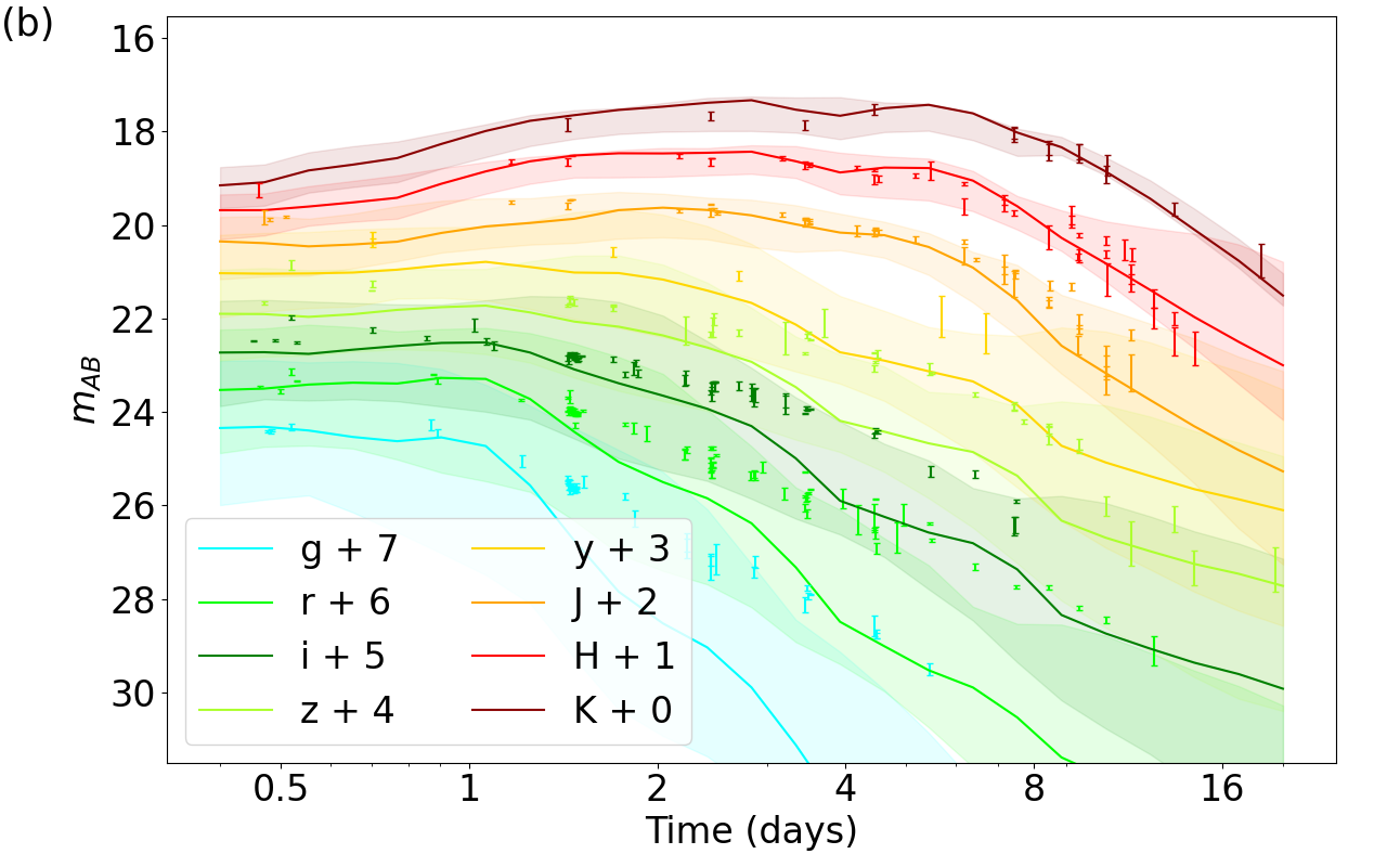
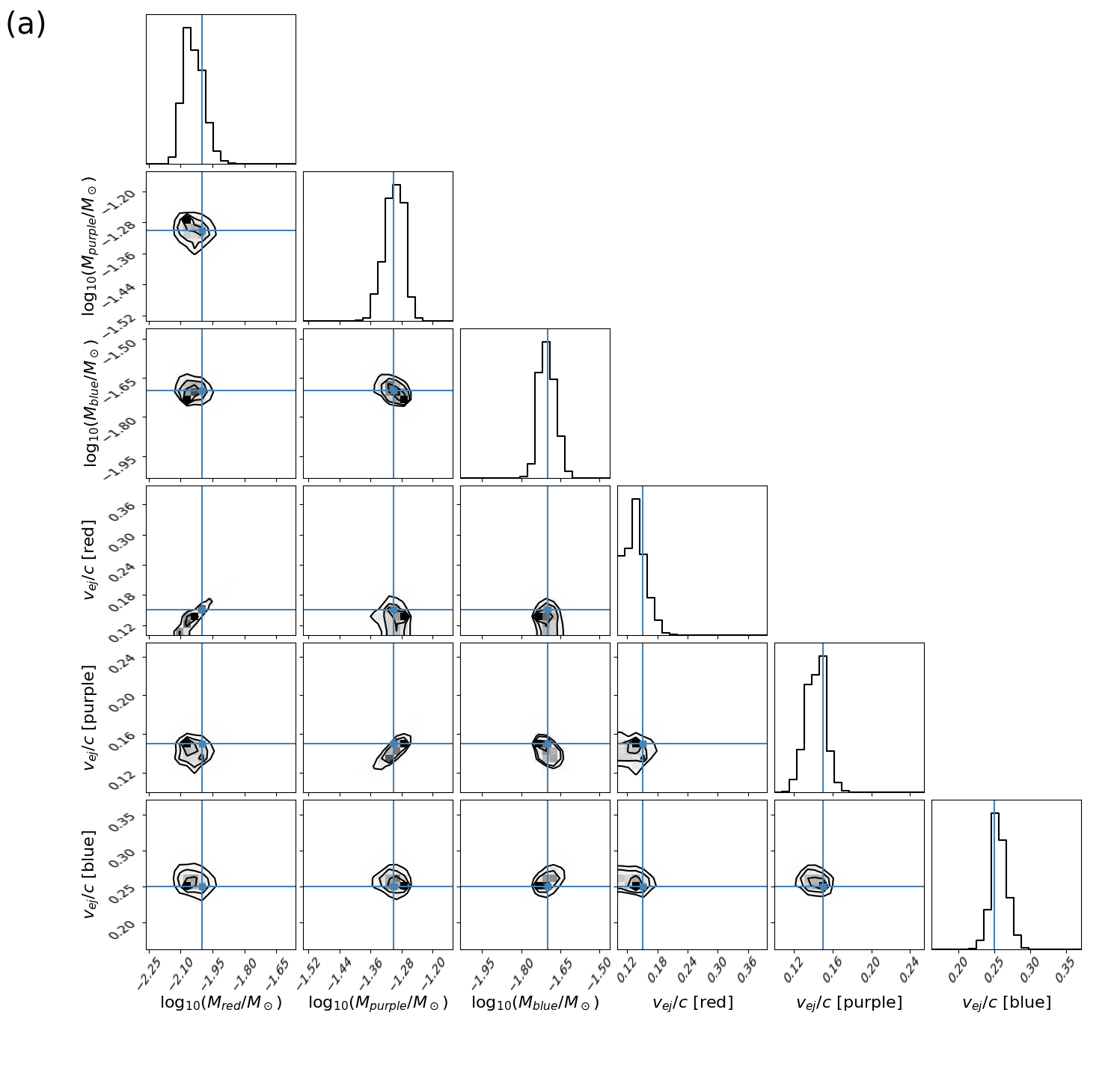
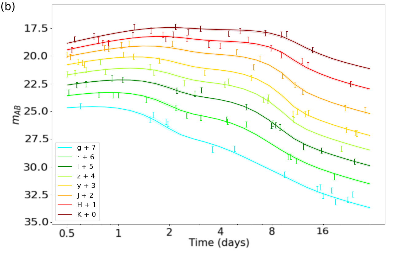
Figure 14 illustrates our implementation of this synthetic model and our parameter inference code. The error bars on the bottom panel show a densely-sampled synthetic multiband light curve with plausible kilonova parameters for all three components. The top panel shows a standard corner plot representing the parameters of our synthetic kilonova with thin blue lines; one-dimensional marginal posterior distributions on the diagonal for each parameter; and two-dimensional marginal posterior distributions in the bottom corner.

Figure 14: Analytic kilonova model injection: Top panel:Posterior distribution for the injection/recovery test (the blue lines show the true parameter values). For this example, $T_{c}$ was fixed for each component and the distance was fixed to 40.0 Mpc. Bottom panel: Fake photometry data and light curve models for the injection/recovery test. The solid line shows the light curve model evaluated at the maximum-likelihood parameters. Both the data and light curves include a confidence interval.

A.3 Validation test: random synthetic kilonova and probability-probability plot

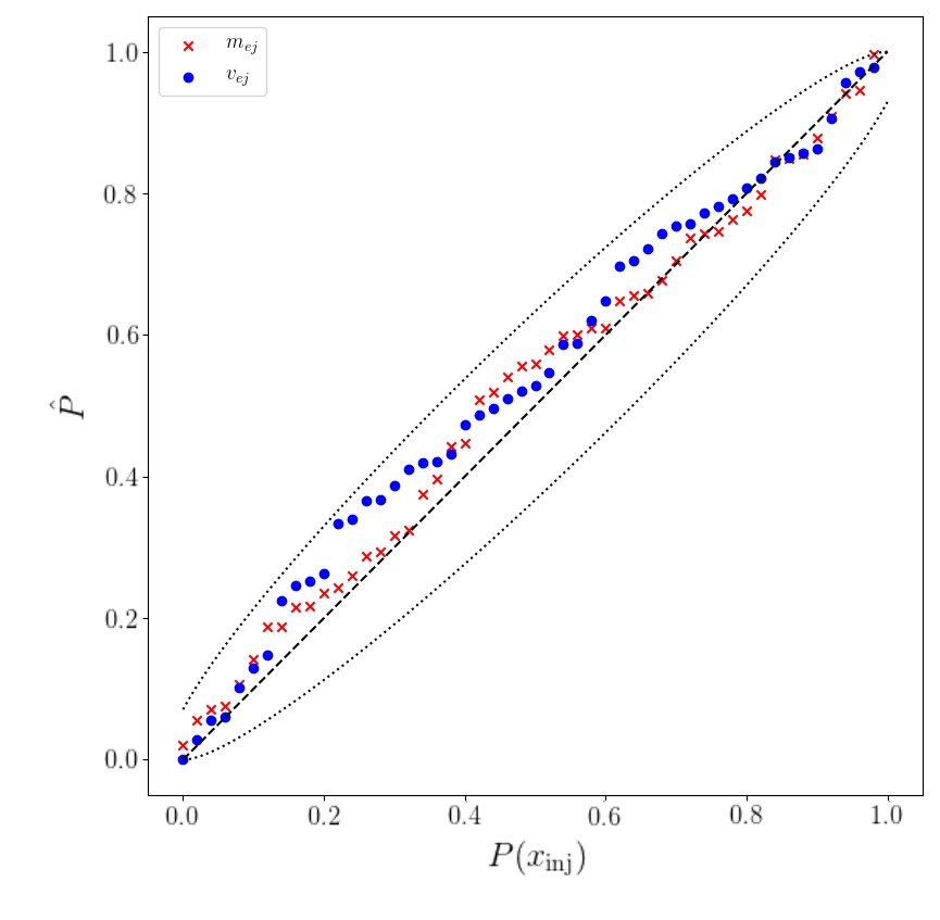
We also demonstrated our inference technique using 100 randomly generated light curves, drawn uniformly from the same priors we use for inference and incorporating noise consistent with our Gaussian noise model. Using these 100 synthetic events and inferences, we can construct a probability-probability (P-P) plot Cook et al. (2012), which corroborates that the one-dimensional marginal distributions are consistent. Figure 15 shows the results of our analysis. More extensive tests of the underlying integration algorithm, including PP plots using more complex and higher dimensional models, are reported elsewhere Champion et al. (2021).

Figure 15: Probability-probability (P-P) tests: P-P plot for 100 synthetic injections generated with one random component.

References

- Abbott et al. (2017) B. P. Abbott, R. Abbott, T. D. Abbott, F. Acernese, K. Ackley, C. Adams, T. Adams, P. Addesso, R. X. Adhikari, V. B. Adya, et al., “Multi-messenger observations of a binary neutron star merger,” The Astrophysical Journal 848, L12 (2017).
- The LIGO Scientific Collaboration et al. (2017a) The LIGO Scientific Collaboration, the Virgo Collaboration, B. P. Abbott, R. Abbott, T. D. Abbott, F. Acernese, K. Ackley, C. Adams, T. Adams, P. Addesso, et al., “GW170817: Observation of gravitational waves from a binary neutron star inspiral,” Phys. Rev. Lett. 119, 161101 (2017a).
- Lattimer and Schramm (1974) J. M. Lattimer and D. N. Schramm, “Black-Hole-Neutron-Star Collisions,” Astrophysical Journal Letters 192, L145 (1974).
- Li and Paczyński (1998) Li-Xin Li and Bohdan Paczyński, “Transient Events from Neutron Star Mergers,” Astrophysical Journal Letters 507, L59–L62 (1998).
- Metzger (2019) Brian D. Metzger, “Kilonovae,” Living Reviews in Relativity 23, 1 (2019).
- Bernuzzi (2020) Sebastiano Bernuzzi, “Neutron star merger remnants,” General Relativity and Gravitation 52, 108 (2020).
- Barnes et al. (2021) Jennifer Barnes, Y. L. Zhu, K. A. Lund, T. M. Sprouse, N. Vassh, G. C. McLaughlin, M. R. Mumpower, and R. Surman, “Kilonovae across the nuclear physics landscape: The impact of nuclear physics uncertainties on r-process-powered emission,” The Astrophysical Journal 918, 44 (2021).
- Zhu et al. (2021) Y. L. Zhu, K. A. Lund, J. Barnes, T. M. Sprouse, N. Vassh, G. C. McLaughlin, M. R. Mumpower, and R. Surman, “Modeling Kilonova Light Curves: Dependence on Nuclear Inputs,” Astrophys. J. 906, 94 (2021).
- Vassh et al. (2021) Nicole Vassh, Gail C. McLaughlin, Matthew R. Mumpower, and Rebecca Surman, “Markov chain monte carlo predictions of neutron-rich lanthanide properties as a probe of r-process dynamics,” The Astrophysical Journal 907, 98 (2021).
- Horowitz (2019) C. J. Horowitz, “Neutron rich matter in the laboratory and in the heavens after GW170817,” Annals of Physics 411, 167992 (2019).
- Chatziioannou (2020) Katerina Chatziioannou, “Neutron-star tidal deformability and equation-of-state constraints,” General Relativity and Gravitation 52, 109 (2020).
- Chen et al. (2021) Hsin-Yu Chen, Philip S. Cowperthwaite, Brian D. Metzger, and Edo Berger, “A program for multimessenger standard siren cosmology in the era of LIGO a, rubin observatory, and beyond,” The Astrophysical Journal 908, L4 (2021).
- Coughlin et al. (2020a) Michael W. Coughlin, Sarah Antier, Tim Dietrich, Ryan J. Foley, Jack Heinzel, Mattia Bulla, Nelson Christensen, David A. Coulter, Lina Issa, and Nandita Khetan, “Measuring the Hubble constant with a sample of kilonovae,” Nature Communications 11, 4129 (2020a).
- Coughlin et al. (2020b) Michael W. Coughlin, Tim Dietrich, Jack Heinzel, Nandita Khetan, Sarah Antier, Mattia Bulla, Nelson Christensen, David A. Coulter, and Ryan J. Foley, “Standardizing kilonovae and their use as standard candles to measure the Hubble constant,” Physical Review Research 2, 022006 (2020b).
- Doctor (2020) Zoheyr Doctor, “Thunder and Lightning: Using Neutron-star Mergers as Simultaneous Standard Candles and Sirens to Measure Cosmological Parameters,” Astrophysical Journal Letters 892, L16 (2020).
- The LIGO Scientific Collaboration et al. (2017b) The LIGO Scientific Collaboration, the Virgo Collaboration, B. P. Abbott, R. Abbott, T. D. Abbott, F. Acernese, K. Ackley, C. Adams, T. Adams, P. Addesso, et al., “Multi-messenger Observations of a Binary Neutron Star Merger,” Astrophysical Journal Letters (2017b), 10.3847/2041-8213/aa91c9.
- The LIGO Scientific Collaboration et al. (2017c) The LIGO Scientific Collaboration, the Virgo Collaboration, B. P. Abbott, R. Abbott, T. D. Abbott, F. Acernese, K. Ackley, C. Adams, T. Adams, P. Addesso, et al., “A standard siren measurement of the Hubble constant,” Nature (London) 551, 85–88 (2017c).
- The LIGO Scientific Collaboration et al. (2018) The LIGO Scientific Collaboration, the Virgo Collaboration, B. P. Abbott, R. Abbott, T. D. Abbott, F. Acernese, K. Ackley, C. Adams, T. Adams, P. Addesso, et al., “GW170817: Measurements of neutron star radii and equation of state,” Phys. Rev. Lett. 121, 161101 (2018).
- The LIGO Scientific Collaboration et al. (2020) The LIGO Scientific Collaboration, the Virgo Collaboration, B. P. Abbott, R. Abbott, T. D. Abbott, S. Abraham, F. Acernese, K. Ackley, C. Adams, V. B. Adya, et al., “Model comparison from LIGO-Virgo data on GW170817’s binary components and consequences for the merger remnant,” Classical and Quantum Gravity 37, 045006 (2020).
- Bauswein et al. (2020) Andreas Bauswein, Sebastian Blacker, Vimal Vijayan, Nikolaos Stergioulas, Katerina Chatziioannou, James A. Clark, Niels-Uwe F. Bastian, David B. Blaschke, Mateusz Cierniak, and Tobias Fischer, “Equation of State Constraints from the Threshold Binary Mass for Prompt Collapse of Neutron Star Mergers,” Phys. Rev. Lett. 125, 141103 (2020).
- Hotokezaka et al. (2019) K. Hotokezaka, E. Nakar, O. Gottlieb, S. Nissanke, K. Masuda, G. Hallinan, K. P. Mooley, and A. T. Deller, “A Hubble constant measurement from superluminal motion of the jet in GW170817,” Nature Astronomy 3, 940–944 (2019).
- Dietrich et al. (2020) Tim Dietrich, Michael W. Coughlin, Peter T. H. Pang, Mattia Bulla, Jack Heinzel, Lina Issa, Ingo Tews, and Sarah Antier, “Multimessenger constraints on the neutron-star equation of state and the Hubble constant,” Science 370, 1450–1453 (2020).
- Coughlin et al. (2018) Michael W. Coughlin, Tim Dietrich, Zoheyr Doctor, Daniel Kasen, Scott Coughlin, Anders Jerkstrand, Giorgos Leloudas, Owen McBrien, Brian D. Metzger, Richard O’Shaughnessy, and Stephen J. Smartt, “Constraints on the neutron star equation of state from AT2017gfo using radiative transfer simulations,” Monthly Notices of the Royal Astronomical Society 480, 3871–3878 (2018).
- Villar et al. (2017) V. A. Villar, J. Guillochon, E. Berger, B. D. Metzger, P. S. Cowperthwaite, M. Nicholl, K. D. Alexand er, P. K. Blanchard, R. Chornock, T. Eftekhari, W. Fong, R. Margutti, and P. K. G. Williams, “The Combined Ultraviolet, Optical, and Near-infrared Light Curves of the Kilonova Associated with the Binary Neutron Star Merger GW170817: Unified Data Set, Analytic Models, and Physical Implications,” Astrophysical Journal Letters 851, L21 (2017).
- Breschi et al. (2021) Matteo Breschi, Albino Perego, Sebastiano Bernuzzi, Walter Del Pozzo, Vsevolod Nedora, David Radice, and Diego Vescovi, “At2017gfo: Bayesian inference and model selection of multicomponent kilonovae and constraints on the neutron star equation of state,” Monthly Notices of the Royal Astronomical Society 505, 1661–1677 (2021).
- Heinzel et al. (2021) J Heinzel, M W Coughlin, T Dietrich, M Bulla, S Antier, N Christensen, D A Coulter, R J Foley, L Issa, and N Khetan, “Comparing inclination-dependent analyses of kilonova transients,” Monthly Notices of the Royal Astronomical Society 502, 3057–3065 (2021).
- Coughlin et al. (2019) Michael W. Coughlin, Tim Dietrich, Ben Margalit, and Brian D. Metzger, “Multimessenger Bayesian parameter inference of a binary neutron star merger,” Monthly Notices of the Royal Astronomical Society 489, L91–L96 (2019).
- Smartt et al. (2017) S. J. Smartt, T. W. Chen, A. Jerkstrand, M. Coughlin, E. Kankare, S. A. Sim, M. Fraser, C. Inserra, K. Maguire, K. C. Chambers, et al., “A kilonova as the electromagnetic counterpart to a gravitational-wave source,” Nature (London) 551, 75–79 (2017).
- Tanvir et al. (2017) N. R. Tanvir, A. J. Levan, C. González-Fernández, O. Korobkin, I. Mandel, S. Rosswog, J. Hjorth, P. D’Avanzo, A. S. Fruchter, C. L. Fryer, et al., “The Emergence of a Lanthanide-rich Kilonova Following the Merger of Two Neutron Stars,” Astrophysical Journal Letters 848, L27 (2017).
- Alexander et al. (2017) K. D. Alexander, E. Berger, W. Fong, P. K. G. Williams, C. Guidorzi, R. Margutti, B. D. Metzger, J. Annis, P. K. Blanchard, D. Brout, et al., “The Electromagnetic Counterpart of the Binary Neutron Star Merger LIGO/Virgo GW170817. VI. Radio Constraints on a Relativistic Jet and Predictions for Late-time Emission from the Kilonova Ejecta,” Astrophysical Journal Letters 848, L21 (2017).
- Chornock et al. (2017) R. Chornock, E. Berger, D. Kasen, P. S. Cowperthwaite, M. Nicholl, V. A. Villar, K. D. Alexander, P. K. Blanchard, T. Eftekhari, W. Fong, et al., “The Electromagnetic Counterpart of the Binary Neutron Star Merger LIGO/Virgo GW170817. IV. Detection of Near-infrared Signatures of r-process Nucleosynthesis with Gemini-South,” Astrophysical Journal Letters 848, L19 (2017).
- Cowperthwaite et al. (2017) P. S. Cowperthwaite, E. Berger, V. A. Villar, B. D. Metzger, M. Nicholl, R. Chornock, P. K. Blanchard, W. Fong, R. Margutti, M. Soares-Santos, et al., “The Electromagnetic Counterpart of the Binary Neutron Star Merger LIGO/Virgo GW170817. II. UV, Optical, and Near-infrared Light Curves and Comparison to Kilonova Models,” Astrophysical Journal Letters 848, L17 (2017).
- Wollaeger et al. (2018) Ryan T. Wollaeger, Oleg Korobkin, Christopher J. Fontes, Stephan K. Rosswog, Wesley P. Even, Christopher L. Fryer, Jesper Sollerman, Aimee L. Hungerford, Daniel R. van Rossum, and Allan B. Wollaber, “Impact of ejecta morphology and composition on the electromagnetic signatures of neutron star mergers,” Monthly Notices of the Royal Astronomical Society 478, 3298–3334 (2018).
- Even et al. (2020) Wesley Even, Oleg Korobkin, Christopher L. Fryer, Christopher J. Fontes, R. T. Wollaeger, Aimee Hungerford, Jonas Lippuner, Jonah Miller, Matthew R. Mumpower, and G. Wendell Misch, “Composition Effects on Kilonova Spectra and Light Curves. I,” Astrophys. J. 899, 24 (2020).
- Wollaeger et al. (2021) R. T. Wollaeger, C. L. Fryer, E. A. Chase, C. J. Fontes, M. Ristic, A. L. Hungerford, O. Korobkin, R. O’Shaughnessy, and A. M. Herring, “A broad grid of 2d kilonova emission models,” The Astrophysical Journal 918, 10 (2021).
- Ristic (2020) Marko Ristic, “Smarter Simulation Placement of Kilonova Light Curve Models for Computationally Inexpensive Surrogate Model Creation,” Thesis, Rochester Institute of Technology (2020).
- Kasen et al. (2017) Daniel Kasen, Brian Metzger, Jennifer Barnes, Eliot Quataert, and Enrico Ramirez-Ruiz, “Origin of the heavy elements in binary neutron-star mergers from a gravitational-wave event,” Nature (London) 551, 80–84 (2017).
- Korobkin et al. (2021) Oleg Korobkin, Ryan T. Wollaeger, Christopher L. Fryer, Aimee L. Hungerford, Stephan Rosswog, Christopher J. Fontes, Matthew R. Mumpower, Eve A. Chase, Wesley P. Even, Jonah Miller, G. Wendell Misch, and Jonas Lippuner, “Axisymmetric radiative transfer models of kilonovae,” The Astrophysical Journal 910, 116 (2021).
- Perego et al. (2017) Albino Perego, David Radice, and Sebastiano Bernuzzi, “AT 2017gfo: An Anisotropic and Three-component Kilonova Counterpart of GW170817,” Astrophysical Journal Letters 850, L37 (2017).
- O’Connor et al. (2020) Brendan O’Connor, Paz Beniamini, and Chryssa Kouveliotou, “Constraints on the circumburst environments of short gamma-ray bursts,” Monthly Notices of the Royal Astronomical Society 495, 4782–4799 (2020).
- O’Connor et al. (2021) B. O’Connor, E. Troja, S. Dichiara, E. A. Chase, G. Ryan, S. B. Cenko, C. L. Fryer, R. Ricci, F. Marshall, C. Kouveliotou, R. T. Wollaeger, C. J. Fontes, O. Korobkin, P. Gatkine, A. Kutyrev, S. Veilleux, N. Kawai, and T. Sakamoto, “A tale of two mergers: constraints on kilonova detection in two short GRBs at z 0.5,” Monthly Notices of the Royal Astronomical Society 502, 1279–1298 (2021).
- Wollaeger and van Rossum (2014) Ryan T. Wollaeger and Daniel R. van Rossum, “Radiation Transport for Explosive Outflows: Opacity Regrouping,” Astroph. J. S. 214, 28 (2014).
- Fontes et al. (2015) C J Fontes, H L Zhang, J Abdallah Jr, R E H Clark, D P Kilcrease, J Colgan, R T Cunningham, P Hakel, N H Magee, and M E Sherrill, “The los alamos suite of relativistic atomic physics codes,” Journal of Physics B: Atomic, Molecular and Optical Physics 48, 144014 (2015).
- Fontes et al. (2020) C. J. Fontes, C. L. Fryer, A. L. Hungerford, R. T. Wollaeger, and O. Korobkin, “A line-binned treatment of opacities for the spectra and light curves from neutron star mergers,” Monthly Notices of the Royal Astronomical Society 493, 4143–4171 (2020).
- Winteler et al. (2012) C. Winteler, R. Käppeli, A. Perego, A. Arcones, N. Vasset, N. Nishimura, M. Liebendörfer, and F. K. Thielemann, “Magnetorotationally Driven Supernovae as the Origin of Early Galaxy r-process Elements?” Astrophysical Journal Letters 750, L22 (2012).
- Barnes et al. (2016) Jennifer Barnes, Daniel Kasen, Meng-Ru Wu, and Gabriel Martínez-Pinedo, “Radioactivity and Thermalization in the Ejecta of Compact Object Mergers and Their Impact on Kilonova Light Curves,” Astrophys. J. 829, 110 (2016).
- Radice et al. (2020) David Radice, Sebastiano Bernuzzi, and Albino Perego, “The Dynamics of Binary Neutron Star Mergers and GW170817,” Annual Review of Nuclear and Particle Science 70, annurev (2020).
- Bessell et al. (1998) M. S. Bessell, F. Castelli, and B. Plez, “Model atmospheres broad-band colors, bolometric corrections and temperature calibrations for O - M stars,” Astronomy and Astrophysics 333, 231–250 (1998).
- Blanton and Roweis (2007) Michael R. Blanton and Sam Roweis, “K-Corrections and Filter Transformations in the Ultraviolet, Optical, and Near-Infrared,” Astronomical Journal 133, 734–754 (2007).
- Hewett et al. (2006) P. C. Hewett, S. J. Warren, S. K. Leggett, and S. T. Hodgkin, “The UKIRT Infrared Deep Sky Survey ZY JHK photometric system: passbands and synthetic colours,” Monthly Notices of the Royal Astronomical Society 367, 454–468 (2006).
- Kasen et al. (2015) Daniel Kasen, Rodrigo Fernández, and Brian D. Metzger, “Kilonova light curves from the disc wind outflows of compact object mergers,” Monthly Notices of the Royal Astronomical Society 450, 1777–1786 (2015).
- Nativi et al. (2021) L. Nativi, M. Bulla, S. Rosswog, C. Lundman, G. Kowal, D. Gizzi, G. P. Lamb, and A. Perego, “Can jets make the radioactively powered emission from neutron star mergers bluer?” Monthly Notices of the Royal Astronomical Society 500, 1772–1783 (2021).
- Klion et al. (2021) Hannah Klion, Paul C. Duffell, Daniel Kasen, and Eliot Quataert, “The effect of jet-ejecta interaction on the viewing angle dependence of kilonova light curves,” Monthly Notices of the Royal Astronomical Society 502, 865–875 (2021).
- Piro et al. (2018) L Piro, E Troja, B Zhang, G Ryan, H van Eerten, R Ricci, M H Wieringa, A Tiengo, N R Butler, S B Cenko, O D Fox, H G Khandrika, G Novara, A Rossi, and T Sakamoto, “A long-lived neutron star merger remnant in GW170817: constraints and clues from X-ray observations,” Monthly Notices of the Royal Astronomical Society 483, 1912–1921 (2018).
- Ai et al. (2018) Shunke Ai, He Gao, Zi-Gao Dai, Xue-Feng Wu, Ang Li, Bing Zhang, and Mu-Zi Li, “The allowed parameter space of a long-lived neutron star as the merger remnant of gw170817,” The Astrophysical Journal 860, 57 (2018).
- Wollaeger et al. (2019) Ryan T. Wollaeger, Chris L. Fryer, Christopher J. Fontes, Jonas Lippuner, W. Thomas Vestrand, Matthew R. Mumpower, Oleg Korobkin, Aimee L. Hungerford, and Wesley P. Even, “Impact of Pulsar and Fallback Sources on Multifrequency Kilonova Models,” Astrophys. J. 880, 22 (2019).
- Kawaguchi et al. (2021) Kyohei Kawaguchi, Sho Fujibayashi, Masaru Shibata, Masaomi Tanaka, and Shinya Wanajo, “A low-mass binary neutron star: Long-term ejecta evolution and kilonovae with weak blue emission,” The Astrophysical Journal 913, 100 (2021).
- Korobkin et al. (2021) Oleg Korobkin, Ryan T. Wollaeger, Christopher L. Fryer, Aimee L. Hungerford, Stephan Rosswog, Christopher J. Fontes, Matthew R. Mumpower, Eve A. Chase, Wesley P. Even, Jonah Miller, G. Wendell Misch, and Jonas Lippuner, “Axisymmetric Radiative Transfer Models of Kilonovae,” Astrophys. J. 910, 116 (2021).
- Darbha and Kasen (2020) Siva Darbha and Daniel Kasen, “Inclination Dependence of Kilonova Light Curves from Globally Aspherical Geometries,” Astrophys. J. 897, 150 (2020).
- Kawaguchi et al. (2020) Kyohei Kawaguchi, Masaru Shibata, and Masaomi Tanaka, “Diversity of Kilonova Light Curves,” Astrophys. J. 889, 171 (2020).
- Breiman (2001) Leo Breiman, “Machine learning, volume 45, number 1 - springerlink,” Machine Learning 45, 5–32 (2001).
- Pedregosa et al. (2011) F. Pedregosa, G. Varoquaux, A. Gramfort, V. Michel, B. Thirion, O. Grisel, M. Blondel, P. Prettenhofer, R. Weiss, V. Dubourg, J. Vanderplas, A. Passos, D. Cournapeau, M. Brucher, M. Perrot, and E. Duchesnay, “Scikit-learn: Machine learning in Python,” Journal of Machine Learning Research 12, 2825–2830 (2011).
- Murphy (2012) Kevin P. Murphy, Machine Learning: A Probabilistic Perspective (The MIT Press, 2012).
- Solomon and Zacks (1970) H. Solomon and S. Zacks, “Optimal Design of Sampling from Finite Populations: A Critical Review and Indication of New Research Areas,” Journal of the American Statistical Association 65, 653 (1970).
- Krause and Guestrin (2007) Andreas Krause and Carlos Guestrin, “Nonmyopic active learning of gaussian processes: an exploration-exploitation approach,” in International Conference on Machine Learning (ICML) (Corvallis, Oregon, 2007).
- Cohn et al. (1996) D.A. Cohn, Z Gahramani, and M.I Jordan, “Active Learning with Statistical Models,” Journal of Artificial Intelligence Research 4, 129–145 (1996).
- Gal et al. (2017) Yarin Gal, Riashat Islam, and Zoubin Ghahramani, “Deep bayesian active learning with image data,” arXiv e-prints (2017).
- MacKay (1992) David J.C. MacKay, “Bayesian methods for adaptive models,” (1992).
- Srinivas et al. (2012) Niranjan Srinivas, Andreas Krause, Sham M. Kakade, and Matthias W. Seeger, “Information-theoretic regret bounds for gaussian process optimization in the bandit setting,” IEEE Transactions on Information Theory 58, 3250–3265 (2012).
- Mockus et al. (1978) J. Mockus, V. Tiesis, and A. Zilinskas, “Toward global optimization,” in The Application of Bayesian Methods for Seeking the Extremum (1978) pp. 117–128.
- Wu and Frazier (2018) Jian Wu and Peter I. Frazier, “The parallel knowledge gradient method for batch bayesian optimization,” arXiv e-prints (2018).
- Field et al. (2014) S. E. Field, C. R. Galley, J. S. Hesthaven, J. Kaye, and M. Tiglio, “Fast Prediction and Evaluation of Gravitational Waveforms Using Surrogate Models,” Physical Review X 4, 031006 (2014).
- Arnett (1980) W. D. Arnett, “Analytic solutions for light curves of supernovae of Type II,” Astrophys. J. 237, 541–549 (1980).
- Arnett (1982) W. D. Arnett, “Type I supernovae. I - Analytic solutions for the early part of the light curve,” Astrophys. J. 253, 785–797 (1982).
- Chatzopoulos et al. (2012) E. Chatzopoulos, J. Craig Wheeler, and J. Vinko, “Generalized Semi-analytical Models of Supernova Light Curves,” The Astrophysical Journal 746, 121 (2012).
- Pankow et al. (2015) C. Pankow, P. Brady, E. Ochsner, and R. O’Shaughnessy, “Novel scheme for rapid parallel parameter estimation of gravitational waves from compact binary coalescences,” Phys. Rev. D 92, 023002 (2015).
- Lange et al. (2018) Jacob Lange, Richard O’Shaughnessy, and Monica Rizzo, “Rapid and accurate parameter inference for coalescing, precessing compact binaries,” arXiv e-prints (2018).
- Champion et al. (2021) E. Champion, V. Delfavero, H. Gallagher, J. Lange, O’Shaughnessy R., J. Wofford, D. Wysocki, and A. Yelikar, in prep (2021).
- Arcavi et al. (2017) Iair Arcavi, Griffin Hosseinzadeh, D. Andrew Howell, Curtis McCully, Dovi Poznanski, Daniel Kasen, Jennifer Barnes, Michael Zaltzman, Sergiy Vasylyev, Dan Maoz, and Stefano Valenti, “Optical emission from a kilonova following a gravitational-wave-detected neutron-star merger,” Nature (London) 551, 64–66 (2017).
- Troja et al. (2017) E. Troja, L. Piro, H. van Eerten, R. T. Wollaeger, M. Im, O. D. Fox, N. R. Butler, S. B. Cenko, T. Sakamoto, C. L. Fryer, et al., “The X-ray counterpart to the gravitational-wave event GW170817,” Nature (London) 551, 71–74 (2017).
- Drout et al. (2017) M. R. Drout, A. L. Piro, B. J. Shappee, C. D. Kilpatrick, J. D. Simon, C. Contreras, D. A. Coulter, R. J. Foley, M. R. Siebert, N. Morrell, et al., “Light curves of the neutron star merger GW170817/SSS17a: Implications for r-process nucleosynthesis,” Science 358, 1570–1574 (2017).
- Valenti et al. (2017) Stefano Valenti, David J. Sand, Sheng Yang, Enrico Cappellaro, Leonardo Tartaglia, Alessandra Corsi, Saurabh W. Jha, Daniel E. Reichart, Joshua Haislip, and Vladimir Kouprianov, “The Discovery of the Electromagnetic Counterpart of GW170817: Kilonova AT 2017gfo/DLT17ck,” Astrophysical Journal Letters 848, L24 (2017).
- Pian et al. (2017) E. Pian, P. D’Avanzo, S. Benetti, M. Branchesi, E. Brocato, S. Campana, E. Cappellaro, S. Covino, V. D’Elia, J. P. U. Fynbo, et al., “Spectroscopic identification of r-process nucleosynthesis in a double neutron-star merger,” Nature (London) 551, 67–70 (2017).
- Kasliwal et al. (2017) M. M. Kasliwal, E. Nakar, L. P. Singer, D. L. Kaplan, D. O. Cook, A. Van Sistine, R. M. Lau, C. Fremling, O. Gottlieb, J. E. Jencson, et al., “Illuminating gravitational waves: A concordant picture of photons from a neutron star merger,” Science 358, 1559–1565 (2017).
- Shappee et al. (2017) B. J. Shappee, J. D. Simon, M. R. Drout, A. L. Piro, N. Morrell, J. L. Prieto, D. Kasen, T. W. S. Holoien, J. A. Kollmeier, D. D. Kelson, et al., “Early spectra of the gravitational wave source GW170817: Evolution of a neutron star merger,” Science 358, 1574–1578 (2017).
- Utsumi et al. (2017) Yousuke Utsumi, Masaomi Tanaka, Nozomu Tominaga, Michitoshi Yoshida, Sudhanshu Barway, Takahiro Nagayama, Tetsuya Zenko, Kentaro Aoki, Takuya Fujiyoshi, Hisanori Furusawa, et al., “J-GEM observations of an electromagnetic counterpart to the neutron star merger GW170817,” PASJ 69, 101 (2017).
- Siegel (2019) Daniel M. Siegel, “GW170817 -the first observed neutron star merger and its kilonova: Implications for the astrophysical site of the r-process,” European Physical Journal A 55, 203 (2019).
- Nicholl et al. (2021) Matt Nicholl, Ben Margalit, Patricia Schmidt, Graham P Smith, Evan J Ridley, and James Nuttall, “Tight multimessenger constraints on the neutron star equation of state from gw170817 and a forward model for kilonova light-curve synthesis,” Monthly Notices of the Royal Astronomical Society 505, 3016–3032 (2021).
- Mooley et al. (2018) K. P. Mooley, A. T. Deller, O. Gottlieb, E. Nakar, G. Hallinan, S. Bourke, D. A. Frail, A. Horesh, A. Corsi, and K. Hotokezaka, “Superluminal motion of a relativistic jet in the neutron-star merger GW170817,” Nature (London) 561, 355–359 (2018).
- Evans et al. (2017) P. A. Evans, S. B. Cenko, J. A. Kennea, S. W. K. Emery, N. P. M. Kuin, O. Korobkin, R. T. Wollaeger, C. L. Fryer, K. K. Madsen, F. A. Harrison, et al., “¡i¿swift¡/i¿ and ¡i¿nustar¡/i¿ observations of gw170817: Detection of a blue kilonova,” Science 358, 1565–1570 (2017).
- Troja et al. (2020) E Troja, H van Eerten, B Zhang, G Ryan, L Piro, R Ricci, B O’Connor, M H Wieringa, S B Cenko, and T Sakamoto, “A thousand days after the merger: Continued X-ray emission from GW170817,” Monthly Notices of the Royal Astronomical Society 498, 5643–5651 (2020).
- Korobkin et al. (2012) O. Korobkin, S. Rosswog, A. Arcones, and C. Winteler, “On the astrophysical robustness of the neutron star merger r-process,” Monthly Notices of the Royal Astronomical Society 426, 1940–1949 (2012).
- Miller et al. (2019) Jonah M. Miller, Benjamin R. Ryan, Joshua C. Dolence, Adam Burrows, Christopher J. Fontes, Christopher L. Fryer, Oleg Korobkin, Jonas Lippuner, Matthew R. Mumpower, and Ryan T. Wollaeger, “Full transport model of GW170817-like disk produces a blue kilonova,” Phys. Rev. D 100, 023008 (2019).
- De and Siegel (2021) Soumi De and Daniel M. Siegel, “Igniting weak interactions in neutron star postmerger accretion disks,” The Astrophysical Journal 921, 94 (2021).
- Sekiguchi et al. (2015) Yuichiro Sekiguchi, Kenta Kiuchi, Koutarou Kyutoku, and Masaru Shibata, “Dynamical mass ejection from binary neutron star mergers: Radiation-hydrodynamics study in general relativity,” Phys. Rev. D 91, 064059 (2015).
- Dietrich et al. (2017) Tim Dietrich, Sebastiano Bernuzzi, and Wolfgang Tichy, “Closed-form tidal approximants for binary neutron star gravitational waveforms constructed from high-resolution numerical relativity simulations,” Phys. Rev. D 96, 121501 (2017).
- Lucca and Sagunski (2020) Matteo Lucca and Laura Sagunski, “The lifetime of binary neutron star merger remnants,” Journal of High Energy Astrophysics 27, 33–37 (2020).
- Krüger and Foucart (2020) Christian J. Krüger and Francois Foucart, “Estimates for disk and ejecta masses produced in compact binary mergers,” Phys. Rev. D 101, 103002 (2020).
- Decoene et al. (2020) V. Decoene, C. Guépin, K. Fang, K. Kotera, and B. D. Metzger, “High-energy neutrinos from fallback accretion of binary neutron star merger remnants,” JCAP 2020, 045 (2020).
- Cook et al. (2012) S. Cook, A. Gelman, and D. Rubin, “Validation of Software for Bayesian Models Using Posterior Quantiles,” Journal of Computational and Graphical Statistics 15, 675 (2012).