Matrix-product state approach to the generalized nuclear pairing Hamiltonian

Abstract

We show that from the point of view of the generalized pairing Hamiltonian, the atomic nucleus is a system with small entanglement and can thus be described efficiently using a one-dimensional tensor network (matrix-product state) despite the presence of long-range interactions. The ground state can be obtained using the density-matrix renormalization group (DMRG) algorithm, which is accurate up to machine precision even for large nuclei, is numerically as cheap as the widely used BCS approach, and does not suffer from any mean-field artefacts.

We apply this framework to compute the even-odd mass differences of all known lead isotopes from ¹⁷⁸Pb to ²²⁰Pb in a very large configuration space of 13 shells between the neutron magic numbers 82 and 184 (i.e., two major shells) and find good agreement with the experiment.

To go beyond the ground state, we calculate the first 100 excited states, as well as the two-neutron removal spectral function of ²¹⁰Pb which relates to a two-neutron pickup experiment. Finally, we treat pairing with non-zero angular momentum and determine the lowest excited states in the full configuration space of one major shell, which we demonstrate for the $N=126$, $Z\geq 82$ isotones.

I Introduction

The atomic nucleus is a many-body problem of interacting fermions. In leading order, these interactions can be accounted for by an effective confining single-particle potential such as the harmonic oscillator or the Woods-Saxon potential [93]. In close analogy to the electronic Fermi sea, the solution to the Schrödinger equation yields two separate Fermi seas for the protons and neutrons. If (effective) spin-orbit coupling is incorporated, one can reproduce the experimentally measured closed-shell structure of the nuclei.

While the single-particle approach is quite successful, a confining potential cannot account for the fact that a short-range attractive two-body interaction prefers the formation of singlet pairs [37, 13, 85]. One of the consequences is that all observed doubly-even nuclei have total spin zero, in opposition to the Hund’s rule in electronic systems where repulsive interactions result in a maximal spin. The pairing effect constitutes the dominant residual interaction, and in order to incorporate it into the theory, one must go beyond the single-particle approach and face the full many-body problem.

A basic model to study the pairing effect was introduced by Richardson [71]. Its Hamiltonian reads:

$$\begin{split}H=d\sum_{j=1}^{L}jn_{j}-G&\sum_{jj^{\prime}}a^{\dagger}_{j\uparrow}a^{\dagger}_{j,\downarrow}a_{j^{\prime},\downarrow}a_{j^{\prime}\uparrow},\end{split}$$ (1)

where $a^{\dagger}_{j\sigma}$ is the creation operator of a spin-$1/2$ particle with spin projection $\sigma=\uparrow,\downarrow$, $n_{j}=\sum_{\sigma}a^{\dagger}_{j\sigma}a_{j\sigma}$ is the particle density in an orbital $j$. There are $L$ equidistant orbitals with some energy spacing $d$ (on the order of MeV for nuclei), and hence the on-site energies $\epsilon_{j}=jd$. The second term with $G>0$ describes attractive pair hopping between all orbitals with equal strength (assumed to be justified if $j$ labels a delocalized eigenstate).

The model is integrable and the solution reduces to a set of algebraic equations [71] closely resembling the Bethe ansatz [11]. It was rediscovered in the context of finite superconducting grains [87, 63], where it can be used for quantitative predictions (e.g. with $d\sim 1\text{meV}$, $G/d\sim 0.2$ for Al grains). In the context of nuclear physics, however, it does not describe any nucleus in particular, but serves as a kind of fundamental demonstration model (akin to the Ising model of condensed matter).

For a quantitative description of a particular nucleus, one needs to use a realistic level scheme $\epsilon_{j}$ (taken from the experiment or computed from an effective single-particle theory). Additional refinement comes from using level-resolved interaction matrix elements $G_{jj^{\prime}}$, whereby the model takes the form:

$$\begin{split}H=\sum_{j,m>0}\epsilon_{j}n_{jm}-&\sum_{jj^{\prime}}G_{jj^{\prime}}\sum_{m>0}\left(-1\right)^{j-m}a^{\dagger}_{jm}a^{\dagger}_{j,-m}\\ \times&\sum_{m^{\prime}>0}\left(-1\right)^{j^{\prime}-m^{\prime}}a_{j^{\prime},-m^{\prime}}a_{j^{\prime}m^{\prime}},\end{split}$$ (2)

with $n_{jm}=a^{\dagger}_{jm}a_{jm}+a^{\dagger}_{j,-m}a_{j,-m}$. Now, $j$ is understood to be a combined index that labels the set of orbitals, each of which has a half-integer angular momentum with projection $m=-j,-j+1,\ldots,+j$ (see Appendix A for more details). The nucleons form singlet pairs and the factor $\left(-1\right)^{j-m}$ is related to the corresponding Clebsch-Gordan coefficient $C^{00}_{jmj,-m}$ (cf. Appendix A). The net effect of the pairing term is that total-singlet states split off and decrease in energy, while the other angular momenta remain degenerate. The model is thus tailored to describe the ground state.

A further sophistication consists in allowing the nucleons to couple to angular momenta $J=2,4,6,\ldots$, leading to:

$$\begin{split}H=\sum_{j,m>0}\epsilon_{j}n_{jm}-&\frac{1}{4}\sum_{J}\sum_{jj^{\prime}}G^{J}_{jj^{\prime}}\\ \times\sum_{M}\sum_{mm^{\prime}nn^{\prime}}&C^{JM}_{jmjn}C^{JM}_{j^{\prime}m^{\prime}j^{\prime}n^{\prime}}~{}a^{\dagger}_{jm}a^{\dagger}_{jn}a_{j^{\prime}n^{\prime}}a_{j^{\prime}m^{\prime}},\end{split}$$ (3)

now with general Clebsch-Gordan coefficients $C^{JM}_{jmjn}$. This allows to treat “rotational bands” of pair excitations with $J>0$.

By adding more and more terms, we go down a hierarchy of models, and eventually we want to solve the generic case

$$\begin{split}H=\sum_{k}\epsilon_{k}n_{k}+\frac{1}{4}\sum_{klmn}V_{klmn}a^{\dagger}_{k}a^{\dagger}_{l}a_{n}a_{m},\end{split}$$ (4)

which would also involve both protons and neutrons. Next, we discuss approaches to diagonalize nuclear many-body Hamiltonians.

Mean field

The pairing of nucleons is analogous to the formation of Cooper pairs of electrons in a conventional superconductor where the attraction is mediated by phonons. The problem of superconductivity was famously solved using mean-field theory by Bardeen, Cooper and Schrieffer (BCS) [7]. Soon after, the BCS theory was imported to the nuclear pairing problem [59, 12] and remains a popular method of choice [14, 74, 10]. However, it has notable shortcomings for the mesoscopic problem of the nucleus. Away from the thermodynamic limit, BCS theory breaks particle number conservation and predicts a phase transition at a critical pairing strength which is absent in nuclei. It also shows deviations in the magnitude of ground-state energies from certain exact results [95]. Some improvement of the BCS theory is possible [8, 73].

Analytical techniques

If the couplings $G_{jj^{\prime}}$ in Eq. (2) are related to the onsite energies $\epsilon_{j}$ in a specific way, the model is analytically solvable [27, 29, 21, 66]. Due to this restriction, however, additional free parameters need to be introduced and fitted to the experiment in order to study real nuclei [28]. We also mention the analytically treatable extended pairing model [60, 61]. While powerful in nature, a common drawback of all of these analytical approaches is the restriction on the model parameters. In this work, we investigate arbitrary pairings $G_{jj^{\prime}}$ and levels $\epsilon_{j}$ where integrability is lost [18, 17, 54].

Exact diagonalization

Finding the ground state in the full Hilbert space is an unbiased method, but limited to a small amount of shells [53]. It works well for the five $j$-shells of the Sn isotopes in the range between $N=50$ and $N=82$ neutrons [95], or for the four $j$-shells of the Ca isotopes above $N=20$ [86], but one soon runs into the exponential barrier of the Hilbert space size for larger nuclei such as lanthanides, Pb, or actinides. Treating such large systems clearly requires an approach that overcomes the exponential barrier, either by truncation or by stochastic probing.

QMC

The stochastic route is taken by various configuration-space quantum Monte Carlo (QMC) techniques [16, 49, 48, 57, 64, 55, 2, 3, 52]. It is well-known that the largest hindrance to the application of Monte Carlo is the infamous sign problem, which is less pronounced for nuclei because the dominant interactions are attractive with the same sign. However, it may still appear for general Hamiltonians that contain repulsive terms (or for odd particle numbers), and requires workarounds [49, 48, 64, 3]. Statistical errors may grow unfavourably, in Ref. [55] as $L^{3}$, reaching the order of $1~{}\text{MeV}$ even for relatively simple models. We also note that early applications of Monte Carlo dealt with constant pairing couplings $G_{jj^{\prime}}\equiv G$, a limitation that was addressed only relatively recently [52].

DMRG

The density matrix renormalization group (DMRG) [91, 75, 76] belongs to the class of approximative wavefunction-based methods. It truncates the Hilbert space to a subset of relevant states based on their entanglement properties. Shortly after its introduction in condensed matter, an early form of DMRG was applied to toy models of nuclear physics, such as pairing in a single shell with a large angular momentum $j=99/2$ [22, 23, 26]. The approach involved specific formulations, dubbed phDMRG or JDMRG rather than the matrix-product state (MPS) formulation [76] that later became the prevalent language in condensed matter. The result was that DMRG can produce machine-precision results for these simple models. We also note the simultaneous application to superconducting grains described by Equation (1) [24, 25, 87, 34, 35] with a similar conclusion. Later, DMRG was applied to the more realistic problem of the pf-shell [62, 67, 83], which contains up to $L_{n}=L_{p}=10$ doubly degenerate neutron and proton orbitals with valence band fillings $N_{\text{val}}=Z_{\text{val}}=4$ for ⁴⁸Cr and $N_{\text{val}}=Z_{\text{val}}=8$ for ⁵⁶Ni. Reference exact solutions exist for this case, allowing to benchmark DMRG. In the first approach, large discrepancy of $0.4~{}\text{MeV}$ was found for ⁵⁶Ni, which hampered further applications. However, algorithmic progress in matrix-product codes over the years led to a re-examination of the problem, resolving the $0.4~{}\text{MeV}$ discrepancy and going further to the fpg-shell for ⁶⁴Ge ($L_{n}=L_{p}=15$, $N_{\text{val}}=Z_{\text{val}}=12$) [51]. A recent proposal involves the combination of DMRG with ab initio calculations of the coupling constants in the sd-shell ($L_{n}=L_{p}=6$) to solve the generic case Equation (4) [84]. Overall, one finds that DMRG is essentially numerically exact for models of the type Equation (1) [87], while it may struggle for the case (4) with generic couplings if the systems are too large.

We propose that instead of jumping to the completely generic case, it stands to reason to slowly increase the complexity of the model and look at the intermediate cases of (2) and (3), where DMRG is expected to still perform very well, which we explore in this paper. A common playground in this context are the magic-shell nuclei, where one can assume spherical symmetry and neglect the interactions between the two nucleon species, solely focusing on the filling of either the neutron or the proton shell. Since Pb is the largest system among these, it lies at the center of our investigation.

This paper is structured as follows. Section II introduces the model and the conventions that are used. In Section III, we explain in detail how the DMRG can be applied to this problem. In Sec. IV, we look at the Sn isotopes as a benchmark. Section V is the main part, where we move to larger Pb and calculate the even-odd mass differences for all of its known isotopes between ¹⁷⁸Pb and ²²⁰Pb. Compared to previous DMRG applications, we thus only look at one nucleon species, but drastically increase the configuration space to 13 $j$-shells, namely all the six $j$-shells between the neutron magic numbers $N=82-126$, as well as all the seven $j$-shells between $N=126-184$, which can accommodate up to 102 particles ($L=51$). We discuss the accuracy of mean field in Sec. VI and briefly revisit the Sn isotopes in Sec. VII. We demonstrate the power of the method to go beyond ground states and calculate up to 100 low-lying states, as well as the two-neutron removal spectral function in Sec. VIII, and discuss going beyond singlet pairing in Sec. IX.

II The Model

We investigate the model (2) that has two essential inputs: (1) The single-particle parameters leading to a particular level structure $\epsilon_{j}$, for which we use the optimized Seminole parametrization [77] of the Woods-Saxon potential. (2) The interaction matrix elements $G_{jj^{\prime}}$ that have to be computed for an effective internucleon interaction $V\left(\mathbf{r}_{1}-\mathbf{r}_{2}\right)$. Here, we employ the ‘delta-force’ or ‘contact interaction’ $V\left(\mathbf{r}_{1}-\mathbf{r}_{2}\right)=V_{0}~{}\delta^{\left(3\right)}\left(\mathbf{r}_{1}-\mathbf{r}_{2}\right)$, which is a reasonable first guess [19, 20, 15, 74, 6, 82, 80]:

$$G_{jj^{\prime}}=G^{J=0}_{jj^{\prime}}=V_{0}~{}\big{<}jj;00\vphantom{\delta^{\left(3\right)}\left(\mathbf{r}_{1}-\mathbf{r}_{2}\right)j^{\prime}j^{\prime};00}\big{|}\delta^{\left(3\right)}\left(\mathbf{r}_{1}-\mathbf{r}_{2}\right)\big{|}j^{\prime}j^{\prime};00\vphantom{jj;00\delta^{\left(3\right)}\left(\mathbf{r}_{1}-\mathbf{r}_{2}\right)}\big{>}.$$ (5)

This expression has to be evaluated using the wavefunctions of the single-particle Schrödinger equation (see Appendix A for more details) paired according to:

$$\big{|}j_{1}j_{2};JM\big{>}=\frac{1}{\sqrt{2}}\sum_{m_{1}m_{2}}C^{JM}_{j_{1}m_{1}j_{2}m_{2}}a^{\dagger}_{j_{1}m_{1}}a^{\dagger}_{j_{2}m_{2}}\big{|}0\big{>}.$$ (6)

$V_{0}=V_{0}^{J=0}$ remains as the only free parameter. This procedure generalizes when studying model Equation 3, which we discuss in Sec. IX.

It is often useful to introduce the pseudospin operators [5]

$$\begin{split}L^{+}_{j}&=\left(L^{-}_{j}\right)^{\dagger}=\frac{1}{2}\sum_{m=-j}^{j}\left(-1\right)^{j-m}a^{\dagger}_{jm}a^{\dagger}_{j,-m},\\ &=\sum_{m>0}\left(-1\right)^{j-m}a^{\dagger}_{jm}a^{\dagger}_{j,-m}\\ L^{z}_{j}&=\frac{1}{2}\sum_{m=-j}^{j}\left(a^{\dagger}_{jm}a_{jm}-\frac{1}{2}\right)\\ &=\frac{1}{2}\sum_{m>0}\left(a^{\dagger}_{jm}a_{jm}+a^{\dagger}_{j,-m}a_{j,-m}-1\right)\\ &=\frac{1}{2}\left(n_{j}-\Omega_{j}\right),\end{split}$$ (7)

with $\Omega_{j}=\left(2j+1\right)/2$ and $n_{j}=\sum_{m}n_{jm}$. They fulfill the SU(2) spin algebra relations $\big{[}L^{+}_{j},L^{-}_{j^{\prime}}\big{]}=2\delta_{jj^{\prime}}L^{z}_{j}$ and $\big{[}L^{z},L^{\pm}_{j^{\prime}}\big{]}=\pm\delta_{jj^{\prime}}L^{\pm}_{j}$. Furthermore, it will be useful to introduce the total pseudospin operators:

$$L^{\pm,z}_{\text{tot}}=\sum_{j}L^{\pm,z}_{j}.$$ (8)

With these operators, the Hamiltonian (2) can be rewritten as

$$H=\sum_{j}\epsilon_{j}\left(2L^{z}_{j}+\Omega_{j}\right)-\sum_{jj^{\prime}}G_{jj^{\prime}}L^{+}_{j}L^{-}_{j^{\prime}},$$ (9)

and particle number conservation translates to a conservation of $L^{z}_{\text{tot}}$.

III Applying DMRG to the nuclear pairing Hamiltonian

III.1 Matrix-product states; mapping to a chain

The DMRG algorithm provides a way to compress the many-body wavefunction [91, 76]. By splitting the system into $L$ sites, each with its local basis $\big{|}\sigma_{l=1\ldots D}\big{>}$ of size $D$, one can transform the basis state coefficients $c_{\sigma_{1}\sigma_{2}\ldots\sigma_{L}}$ into a product of matrices:

$$\begin{split}\big{|}\Psi\big{>}&=\sum_{\boldsymbol{\sigma}}c_{\sigma_{1}\sigma_{2}\ldots\sigma_{L}}\big{|}\sigma_{1}\big{>}\big{|}\sigma_{2}\big{>}\ldots\big{|}\sigma_{L}\big{>}\\ &=\text{Tr}\sum_{\boldsymbol{\sigma}}\underline{A}^{\sigma_{1}}\underline{A}^{\sigma_{2}}\ldots\underline{A}^{\sigma_{L}}\big{|}\sigma_{1}\big{>}\big{|}\sigma_{2}\big{>}\ldots\big{|}\sigma_{L}\big{>}.\end{split}$$ (10)

The key adavantage of such an MPS representation is the notion of locality: The matrix $\underline{A}^{\sigma_{l}}$ associated with the site $\big{|}\sigma_{l}\big{>}$ depends on $\sigma_{l}$ only, and this is the very reason why states with certain entanglement properties can be efficiency encoded (see the next subsection). The concrete choice of the ‘site’ $\big{|}\sigma_{l}\big{>}$ is in principle arbitrary and determined by practicality (it can be as small as a single orbital).

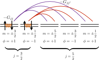
In our case, it is convenient to group the time-conjugate Kramers pairs with $\pm m$ (where $m>0$) into one site, with the local basis given by the following $D=4$ states: the vacuum (pseudospin-down) $\big{|}0\big{>}_{jm}=\big{|}\Downarrow\big{>}_{jm}=\big{|}0\big{>}$, the singly occupied states $\big{|}\uparrow\big{>}_{jm}=a^{\dagger}_{jm}\big{|}0\big{>}$ as well as $\big{|}\downarrow\big{>}_{jm}=a^{\dagger}_{j,-m}\big{|}0\big{>}$, and the doubly occupied (pseudospin-up) state $\big{|}\uparrow\downarrow\big{>}_{jm}=\big{|}\Uparrow\big{>}_{jm}=a^{\dagger}_{jm}a^{\dagger}_{j,-m}\big{|}0\big{>}$. The factor $\left(-1\right)^{j-m}$ is absorbed into the Hamiltonian. Thus, a $j$-shell corresponds to $\Omega_{j}=j+1/2$ sites with energy $\epsilon_{j}$. All of the sites are sequentially enumerated, so that the whole problem is mapped onto a one-dimensional chain of length $L=\sum_{j}\Omega_{j}$. This is illustrated in Figure 1.

Figure 1: The nuclear pairing Hamiltonian in Equation (2) can be mapped to a one-dimensional chain, which can subsequently be treated using matrix-product states. This is illustrated here for the case of two nuclear levels with $j=\frac{3}{2}$ and $j=\frac{5}{2}$, which are mapped onto a chain of length $L=5$. The arched lines indicate the long-range pair hopping $-G_{jj^{\prime}}$ between the sites with an additional phase $\phi=\left(-1\right)^{j-m}$ ($m>0$) for each site.

III.2 Entanglement entropy

Equation (10) is exact if the matrices are not truncated; in order to represent an arbitrary state, exponentially large matrices of size up to $D^{L/2}$ are necessary. At the heart of the DMRG algorithm lies the observation that a large class of physical states can in fact be expressed by matrices of a much smaller size $\chi\ll D^{L/2}$ (called the ‘bond dimension’) without introducing much error. The value $\chi$ is a measure of the number of variational parameters that are used to represent the wavefunction. It is also a measure of the numerical effort, since the largest matrix that must be handled is of size $\chi\times\chi$. The maximal value that can be treated in typical DMRG calculations is $\chi\sim 10^{4}$.

The reason why many physical states can be efficiently represented by an MPS is related to the notion of entanglement. To quantify this, one divides the chain into two parts A and B and integrates out part B, resulting in a mixed state:

$$\rho_{A}=\text{Tr}_{B}\big{|}\Psi\big{>}\big{<}\Psi\big{|}.$$ (11)

The quantity that characterizes the entanglement of this bipartition is the entanglement entropy

$$S_{A|B}=-\text{Tr}\rho_{A}\ln\rho_{A},$$ (12)

which is granted as a byproduct in the DMRG algorithm. The crucial question is thus how $S_{A|B}$ scales with the number of particles. For gapped one-dimensional models with short-range interactions, the so-called area law guarantees that $S_{A|B}$ stays constant [30], so that the numerical effort grows only linearly.

The nuclear pairing problem features long-range interactions, and the existence of an area law is not guaranteed. Even though the system is finite, the amount of entanglement (and thus $\chi$) might still be prohibitively large. However, we in fact find that the ground state does indeed have a very low entanglement and can be represented by a rather small $\chi\sim 10^{2}$ to nearly machine precision. The reason is that the nucleus is in the weak-coupling regime and the deep $j$-shells in the left part of the chain are almost completely filled, forming a weakly entangled near-product state, while the right part of the chain is mostly empty, with only few excitations across a softened Fermi edge that contribute to the entanglement. This will be demonstrated explicitly in Sec. V.

Finally, we emphasize that the DMRG approach does not neglect any diagrams and does not rely on particle-hole excitation cutoffs as, e.g., in the configuration interaction approach [38]. If a good MPS representation of the ground state can be found, the result becomes numerically exact.

III.3 Matrix-product operators

In order to implement the DMRG algorithm, we also need to express the Hamiltonian in a form analogous to the one of the wavefunction in Equation (10). This is achieved by a matrix-product operator (MPO) representation:

$$H=\sum_{\boldsymbol{\sigma}\boldsymbol{\sigma}^{\prime}}\text{Tr}~{}\underline{W}^{\sigma_{1}\sigma_{1}^{\prime}}\ldots\underline{W}^{\sigma_{L}\sigma_{L}^{\prime}}\big{|}\sigma_{1}\big{>}\ldots\big{|}\sigma_{L}\big{>}\big{<}\sigma_{1}^{\prime}\big{|}\ldots\big{<}\sigma_{L}^{\prime}\big{|},$$ (13)

where the coefficients $\underline{W}^{\sigma_{i}\sigma_{i}^{\prime}}$ can be determined analytically for any given $H$ [76]. However, the bond dimension $\chi_{\text{MPO}}$ of the MPO (the size of the matrices $\underline{W}$) can in general be prohibitively large, in particular if the Hamiltonian contains long-range interactions. We address this problem by applying a lossless MPO compression algorithm [41] that exploits linear dependencies in the matrices to reduce $\chi_{\text{MPO}}$. We find a reduction by as much as $99\%$ from the naive construction; the runtime of this algorithm is a few seconds. We point out that no approximation is introduced by this compression procedure.

The massive reduction of $\chi_{\text{MPO}}$ is probably a specific feature of the nuclear pairing Hamiltonian and likely related to the fact that the interaction terms are the same for all sites between fixed $j$ and $j^{\prime}$. We suspect that the efficient representation can also be found analytically in the case of singlet pairing. Note that in the Richardson model (1), where $G_{jj^{\prime}}\equiv G$, only the total pseudospinflip operators Equation (8) couple to each other in the form $-GL^{+}_{\text{tot}}L^{-}_{\text{tot}}$. A sum of local operators such as $L^{+}_{\text{tot}}$ has an analytical MPO representation with $\chi_{\text{MPO}}=2$, and the product $L^{+}_{\text{tot}}L^{-}_{\text{tot}}$ is at most described by $\chi_{\text{MPO}}=4$ [65]. However, if more complicated terms are added to the Hamiltonian (like the pairing to $J>0$ considered in Sec. IX), analytical approaches become too cumbersome and the numerical compression that we use becomes indispensable.

III.4 Implementation

The core idea of a ground-state DMRG algorithm is to locally optimize the tensors $\underline{A}^{\sigma_{i}}$ from Equation (10) using the Ritz variational principle [91, 75, 76]. In the presence of symmetries the tensors acquire a block structure and the algorithm has to distribute the available bond dimension among these blocks. For this, we use the subspace expansion method of the 1-site algorithm described in Ref. [40].

As a measure of convergence we use the energy variance per particle

$$\Delta E^{2}/N=\left(\big{<}H^{2}\big{>}-E^{2}\right)/N,$$ (14)

which indicates how close we are to an eigenstate.

In condensed-matter language, the Hamiltonian in Equation (2) is mapped to a chain of fermionic orbital pairs with on-site energies $\epsilon_{j}$, an on-site attractive Hubbard term $-G_{jj}n_{jm}n_{j,-m}$, and attractive pair hoppings between all sites (see Figure 1). Since the single-band Hubbard model is a standard application for the DMRG method, we point out that the code can be implemented without any significant modification of standard algorithms, with the exception of the MPO representation of the Hamiltonian. For this, either a compact analytical expression must be found, or it has to be compressed numerically. Another obstacle is the impeded convergence due to the slightly pathological nature of the Hamiltonian (2). We discuss how it can be resolved in Appendix B.

IV Benchmark: the tin isotopes

Figure 2: The Sn isotopes serve as a benchmark case for the DMRG algorithm. The even-odd mass differences (15) as well as the staggered variant (16) are compared to experimental data [88] and exact diagonalization (ED) results; the latter are reproduced by the DMRG to 10 relevant digits. The single-particle levels $\epsilon_{j}$ as the interaction matrix elements $G_{jj^{\prime}}$ are taken from Ref. [95]. The grey and purple shaded areas indicates closed shells and half filling, respectively.

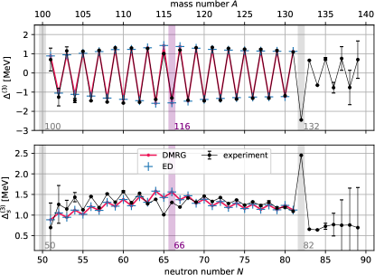
It is instructive to study a drosophila scenario to benchmark the DMRG algorithm. To this end, we consider pairing in the Sn isotopes, which can still be treated using exact diagonalization [39] and which frequently serves as a testing ground for approximate techniques [95, 73, 17]. The on-site energies $\epsilon_{j}$ are taken from the experiment, and the interaction parameters $G_{jj^{\prime}}$ result from G-matrix calculations [95]. The system is assumed to have an inert core with $Z=50$ protons and $N=50$ neutrons. The valence neutrons fill the shells $1g_{7/2}$, $2d_{5/2}$, $2d_{3/2}$, $3s_{1/2}$, and $1h_{11/2}$ from $N=50$ to $N=82$. In our nomenclature, this corresponds to a chain of $L=16$ sites. To fix the filling, we only exploit the conservation of the particle number (U(1) charge symmetry).

The MPO associated with the Hamiltonian of the Sn isotopes can be compressed exactly in under 0.1s runtime from the maximal bond dimension of $\chi_{\text{MPO}}=130$ down to $\chi_{\text{MPO}}=8$. The ground state search is most difficult around half filling ($N=66$ or 16 fermions in the chain), but the runtime is still less than 1s on a regular desktop computer. The MPS bond dimension is at most $\chi\sim 50$. The variance per particle (Equation (14)) is of the order of $10^{-9}~{}\text{MeV}^{2}$ or smaller, so that we can be confident to have well-converged results.

Figure 3: The even-odd mass differences [see Eqs. (15) and (16)] are calculated using the DMRG for the lead isotopes. We use a large configuration space that includes all shells between $N=82$ and $N=184$. Their energies $\epsilon_{j}$ are determined by solving the single-particle Hamiltonian Equation (21) in the Seminole parametrization. The pairing strength $V_{0}$ is the only free parameter, see Equation (5). For $V_{0}=250~{}\text{MeV}$, we find excellent agreement with the experimental data [88].

A quantity that demonstrates the even-odd effect due to pairing is the discrete derivative of the ground-state energy with respect to the particle number, which we compute via the 3-point rule [9]

$$\Delta^{\left(3\right)}\left(N\right)=E_{0}\left(N\right)-\left[E_{0}\left(N-1\right)+E_{0}\left(N+1\right)\right]/2.$$ (15)

This is known as the ‘even-odd mass difference’. In condensed matter, it is referred to as the ‘pair binding energy’ and is connected to superconductivity of coupled molecules [92]. One can also add a staggered factor that makes all values positive:

$$\Delta_{s}^{\left(3\right)}\left(N\right)=\left(-1\right)^{N+1}\Delta^{\left(3\right)}\left(N\right).$$ (16)

The result is shown in Figure 2; exact diagonalization data are reproduced to at least 10 digits. We also show experimental results  [88]. The agreement between theory and experiment is noticeably worse around half filling, where there is a gap between $2d_{5/2}$ and $3s_{1/2}$ in the single-particle energies. This can be improved upon in our approach (see Sec. VII).

V The lead isotopes

We now turn to the Pb isotopes. We assume an inert core of $Z=82$ protons and $N=82$ neutrons and include all the shells between $N=82$ and $N=126$ into our parameter space ($2f_{7/2}$, $1h_{9/2}$, $1i_{13/2}$, $3p_{3/2}$, $2f_{5/2}$, $3p_{1/2}$), as well as all the shells up to the next magic number $N=184$ ($2g_{9/2}$, $1i_{11/2}$, $1j_{15/2}$, $3d_{5/2}$, $4s_{1/2}$, $2g_{7/2}$, $2d_{3/2}$). This is a very large configuration space that corresponds to a chain length of $L=51$. The half filling point of the $N=82-126$ major shell is given by $N=104$ (¹⁸⁶Pb), or by 22 fermions in the chain. The smallest and largest known isotopes are ¹⁷⁸Pb and ²²⁰Pb [88], respectively (corresponding to 14 and 56 fermions in the chain). The energies $\epsilon_{j}$ are now taken from the numerical solution of the single-particle Schrödinger equation, and the pairing strength $V_{0}$ is the only free parameter in the calculation, see Equation (5). Note that large-scale ED shell model calculations have been performed for this system for doping of up to 14 neutrons away from the magic $N=126$ shell, i.e. $\Delta^{\left(3\right)}$ has been computed in a range of $N=114-126$ [69].

The MPO representation of the Hamiltonian for this much larger system can be again compressed from the naive setup that results in $\chi_{\text{MPO}}=1302$ down to $\chi_{\text{MPO}}=16$. An MPS bond dimension of around $\chi\sim 250$ is sufficient to faithfully represent the ground state at intermediate fillings, and the variance per particle Equation (14) is again at worst of the order of $10^{-9}~{}\text{MeV}^{2}$. The calculation takes about 1-2 minutes on a desktop computer.

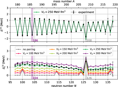
The results for the even-odd mass difference $\Delta^{\left(3\right)}$ are displayed in Figure 3. We find that a pairing strength of $V_{0}=250~{}\text{MeV}~{}\text{fm}^{3}$ yields excellent agreement with the experimental data [88] despite the simplicity of the delta-force interaction. This can be quantified by introducing

$$\sigma=\sqrt{\frac{\sum_{N=N_{\text{min}}}^{N_{\text{max}}}\left(\Delta^{\left(3\right)}_{\text{theory}}\left(N\right)-\Delta^{\left(3\right)}_{\text{exper.}}\left(N\right)\right)^{2}}{N_{\text{max}}-N_{\text{min}}}},$$ (17)

and we find $\sigma\approx 0.13~{}\text{MeV}$ (for the Sn benchmark, the corresponding value is $\sigma\approx 0.16~{}\text{MeV}$). This should be compared to the scale of $\Delta^{\left(3\right)}$, which is of the order of $1~{}\text{MeV}$. The value of $\Delta^{\left(3\right)}$ at the closing of the magic shell is insensitive to pairing and is mostly determined by the quality of the single-particle energies $\epsilon_{j}$.

Figure 4: Occupation numbers $\big{<}n_{j}\big{>}$ for ¹⁸⁶Pb and ¹⁹⁷Pb at $V_{0}=250~{}\text{MeV}~{}\text{fm}^{3}$ as computed with the DMRG. The scale of the y-axis for the levels below (above) the magic number $N=126$ is shown on the left (right) side. The location of the gap is marked by the vertical line and grey shading indicates the maximum shell capacity.

Figure 5: The same as in Figure 4 but for all neutron fillings between $N=82$ and $N=184$ of the Pb isotopes. Red (blue) colors indicate the shells below (above) the magic gap. The gap itself is indicated by the black vertical line. The known Pb isotopes have neutron numbers within the white area.

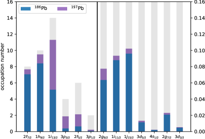
Next, we examine the softening of the Fermi edge due to pairing by computing the occupation numbers $\big{<}n_{j}\big{>}=\sum_{m>0}\big{<}n_{jm}\big{>}$ of each $j$-shell. The results for half filling and 3/4 filling are shown in Figure 4. One observes that it is favourable not to fill the lowest two shells completely before putting a significant number of neutrons into the third $1i_{13/2}$ shell. Furthermore, it is favourable to place a small number of neutrons into much higher shells (even across the magic gap), in particular for high angular momenta.

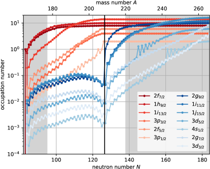
Figure 5 shows all occupation numbers as a function of $N$. We find that an occupation of around $\big{<}n_{j}\big{>}\sim 10^{-1}-10^{-2}$ is kept in the high-$j$ levels $2g_{9/2}$, $1i_{11/2}$, $1j_{15/2}$ before the ²⁰⁸Pb magic shell is filled. Apart from some even-odd oscillations, the rate of filling follows two different laws: The deep shells ($2f_{7/2}$, $1h_{9/2}$ below the magic gap and $2g_{9/2}$, $1i_{11/2}$, $1j_{15/2}$ above it) are filled very rapidly at first and then cross over to a slow saturation. The higher shells are filled exponentially (as seen by the straight lines in the logarithmic plot). Their occupancy is thus exponentially suppressed at first and then steeply increases. This is most extreme in the case of the $3p_{1/2}$ level, which has the smallest pairing overlap with the other shells. The filling of this level abruptly changes by one between $N=125$ and shell closure at $N=126$. This ‘rapid filling’ effect is responsible for the dip in the $\Delta^{\left(3\right)}$ curve at $N=125$ [72].

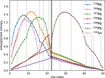
Finally, we compute the entanglement entropy Equation (12) between the lower and higher single-particle orbitals, or equivalently, between the left and right part of the chain. The result is shown in Figure 6. Not surprisingly, the largest values of $S_{A|B}\approx 1.4$ are found for open-shell isotopes ¹⁸⁶Pb and ²²⁰Pb, while the closed-shell ²⁰⁸Pb only has maximal value of around $S_{A|B}\approx 0.3$. One should note that even $S_{A|B}\approx 1.4$ is still only a modest increase compared to $S_{A|B}=\ln\left(2\right)\approx 0.693$ for a pure singlet state. Furthermore, there is only little change between the half-filled ¹¹⁶Sn with 16 neutrons and the half-filled ¹⁸⁶Pb with 22 neutrons. We see that the nuclear shell structure acts as a natural ‘entanglement barrier’: Beyond half filling, the shell starts to close again and the entanglement decreases as the wavefunction gets closer to a product state. Since entanglement depends on the choice of basis, we conclude that the Woods-Saxon basis of the effective shell models is already a very good choice to minimize it. Coupled with the possibility to represent Hamiltonians in Eqs. 1, 2, 3 by only moderately-sized MPOs, this explains the very good performance of DMRG for these systems.

Figure 6: Entanglement entropy (12) for different bipartitions on the chain geometry (the lower single-particle orbitals are to the left) for various Pb isotopes as well as for the half-filled ¹¹⁶Sn. Closures of the various $j$-shells of Pb are indicated by the dotted vertical lines. The Pb magic gap is indicated by the solid vertical line.

VI Comparison with mean field

In this section we address the deviations of our approach from mean field theory (BCS), where the pairing terms are replaced by averages and a quadratic Hamiltonian remains. It is known that for the Richardson model (1), mean field becomes a good approximation for large $L$ (at half filling) or large $G$ [24, 87], as both limits lead to the bulk superconducting gap $\Delta_{\text{BCS}}$ to dominate over the finite-size spacing $d$, i.e. $\Delta_{\text{BCS}}\gg d$. However, for model (2) it is a priori not clear what happens, as a larger nucleus also leads to a weaker coupling because of a smaller radial overlap [13], so that the two effects are to some degree compensatory. Note that the previously obtained optimal coupling value for Pb $V_{0}=250~{}\text{MeV}~{}\text{fm}^{3}$ has be be multiplied with the interaction matrix elements, so that we find that the actual pair hopping strength $G_{jj^{\prime}}$ is in the range of $0.03-0.29~{}\text{MeV}$, compared to $0.15-0.72~{}\text{MeV}$ for Sn.

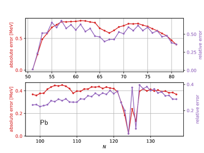
Figure 7 shows the deviation of $\Delta^{(3)}$ between the BCS result and the DMRG result (which we take as the exact value). We see that it becomes somewhat smaller for Pb, but still reaches a value of $0.4~{}\text{MeV}$ in absolute terms, or up to 40% in relative terms. Thus, BCS does not tie with DMRG in terms of accuracy even for large nuclei. Normally, the appeal to use BCS is the cheap numerics, but we find that DMRG is able to provide the exact solution at essentially the same numerical cost.

Figure 7: Absolute (left scale) and relative (right scale) error of the BCS computation for $\Delta^{\left(3\right)}\left(N\right)$, Eq. (15) for $V_{0}=250~{}\text{MeV}~{}\text{fm}^{3}$. We take the DMRG result as the exact reference value.

VII The tin isotopes revisited

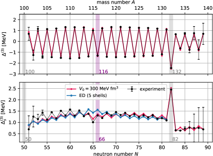
We now revisit the Sn isotopes and try to improve the agreement with the experimental data by extending the parameter space from five shells to all bound eigenstates above $N=50$. To this end, we add $2f_{7/2}$, $3p_{3/2}$, $3p_{1/2}$, $1h_{9/2}$, and $2f_{5/2}$ ($1i_{13/2}$ turns out to be unbound) to the configuration space, resulting in a chain of $L=31$ sites. The shell energies $\epsilon_{j}$ are now determined via the single-particle Hamiltonian as described in Appendix A and the pairing strength $V_{0}$ is a free parameter. The result is shown in Figure 8 for the optimal $V_{0}=300~{}\text{MeV}~{}\text{fm}^{3}$. The average deviation from the experimental values has now decreased to $\sigma\approx 0.10~{}\text{MeV}$. In particular, the dip around half filling is captured more accurately. Moreover, we can compare with the neutron-rich isotopes up to ¹⁴⁰Sn that were not considered previously using ED, and still find excellent agreement with the experiment [88].

Figure 8: Even-odd mass differences of Sn calculated with the DMRG for a large configuration space that includes 10 $j$-shells between the magic numbers $N=50$ and $N=126$ (all bound eigenstates). The shell energies $\epsilon_{j}$ are determined via the single-particle Hamiltonian Equation (2), the pairing strength $V_{0}$ is a free parameter. The agreement between theory and experiment is significantly better than the typically used benchmark dataset in Figure 2, where only five shells were included in the calculation (‘ED’ shows the same dataset as in Figure 2).

VIII Excited states, Two-neutron removal spectral function

We now explore the potential of our approach to compute excited states. We first discuss to which extent the phenomenological pairing Hamiltonian Equation (2) is suited for this purpose.

Pictorially speaking, one can obtain an excited state of a nucleus by promoting a pair to higher angular momentum, by exciting it to a higher level, or by breaking it up. Protons can be excited along neutrons and interact with them, leaving the nucleus deformed, which leads to further complications [72]. The $J=0$ pairing Hamiltonian is tailored to describe the ground state: It only pulls the many-body eigenstates with $J=0$ down in energy but leaves the other eigenstates highly degenerate.

However, it is reasonable to investigate to which degree the Hamiltonian (2) also captures pair excitations with $J=0$. A particularly interesting system is ²⁰⁸Pb where such ‘pair vibrations’ arise across the magic gap and can be probed by two-neutron pickup and stripping experiments: A proton that passes by a nucleus can pick up two neutrons and end up as a triton [43]. Vice versa, two neutrons may be stripped and added to the nucleus [1]. (Note that the condensed matter electronic equivalents are the Auger Electron Spectroscopy and the Appearance Potential Spectroscopy [90, 68, 32, 70].) By choosing ²¹⁰Pb and ²⁰⁶Pb as targets, one can thus specifically study the excited neutron states of ²⁰⁸Pb. If a pair is taken out above (below) the magic gap of ²¹⁰Pb, the nucleus should essentially end up in the ground state (an excited state) of ²⁰⁸Pb.

Within the DMRG, the lowest eigenstates can be constructed by first finding the ground state $\big{|}E_{0}\big{>}$ and then altering the Hamiltonian to $\tilde{H}=H+E_{p}\big{|}E_{0}\big{>}\big{<}E_{0}\big{|}$ with a suitably high energy penalty $E_{p}$. This lifts the ground state in energy by $E_{p}$, and the ground state of $\tilde{H}$ will be the first excited eigenstate $\big{|}E_{1}\big{>}$. The procedure can then be iterated.

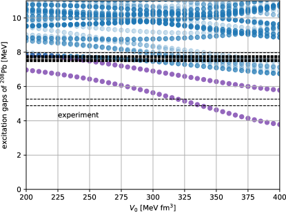
Figure 9 shows the first 100 eigenenergies relative to the ground state of the pairing Hamiltonian for ²⁰⁸Pb as a function of $V_{0}$ within our parameter space of 13 $j$-shells. For comparison, we plot the energies of the singlet states measured experimentally [79]. Theory predicts that as the pairing strength $V_{0}$ is increased, two non-degenerate singlet states split off from a quasi-continuum of other excitations. This is compatible with the experiment where one finds two singlet excitations with $E-E_{0}=4.868~{}\text{MeV}$ and $E-E_{0}=5.241~{}\text{MeV}$ that lie below a dense sequence of singlets around $E-E_{0}\approx 8~{}\text{MeV}$. In order to quantitatively reproduce the energy of the lower singlet, one needs to choose a pairing strength of $V_{0}\approx 340~{}\text{MeV}~{}\text{fm}^{3}$, which is larger than the optimal value of $V_{0}\approx 250~{}\text{MeV}~{}\text{fm}^{3}$ that was found in the ground-state calculation. Given the simplicity of the pairing Hamiltonian, the agreement is thus only qualitative.

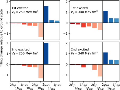
It is instructive to plot the filling of the single-particle levels relative to the ground state, $\big{<}E_{n}\vphantom{n_{j}E_{n}}\big{|}n_{j}\big{|}E_{n}\vphantom{E_{n}n_{j}}\big{>}-\big{<}E_{0}\vphantom{n_{j}E_{0}}\big{|}n_{j}\big{|}E_{0}\vphantom{E_{0}n_{j}}\big{>}$, see Figure 10. For a pairing strength of $V_{0}\approx 250~{}\text{MeV}~{}\text{fm}^{3}$, the excitations are characterized by a transfer of one pair mostly from the highest occupied $3p_{1/2}$ level to the lowest unoccupied $2g_{9/2}$ level. For $V_{0}\approx 340~{}\text{MeV}~{}\text{fm}^{3}$, the levels below the magic gap contribute more equally to the excited state, and the levels above the gap are more strongly hybridized. In the latter case, it is essential to work with a configuration space that is as large as ours.

Figure 9: DMRG data for the energies of the first 100 excited states of the pairing Hamiltonian Equation (2) relative to the ground state as a function of the coupling strength $V_{0}$ for ²⁰⁸Pb. The lowest two singlet states are marked in purple. In all other cases, a stronger colour saturation indicates larger degeneracy. The dashed horizontal lines mark experimentally measured excitation gaps of singlet states [79]. The lowest two can be observed in two-neutron pickup experiments.

In two-neutron pickup experiments, the two singlets are observed with a cross section ratio of about 10:1 [43]. Furthermore, the $E-E_{0}=4.868~{}\text{MeV}$ excitation has a much larger cross section than the ground state. We can check to what degree these results are reproduced by the theory. In a first approximation that neglects the details of the scattering process, we can consider the two-neutron removal spectral function, which we define as [56, 33, 4]:

$$S^{-}\left(E\right)=\sum_{n}\big{|}\big{<}E_{n}^{N-2}\vphantom{L^{-}_{\text{tot}}E_{0}^{N}}\big{|}L^{-}_{\text{tot}}\big{|}E_{0}^{N}\vphantom{E_{n}^{N-2}L^{-}_{\text{tot}}}\big{>}\big{|}^{2}~{}\delta\left(E-E_{0}^{N-2}+E_{n}^{N-2}\right).$$ (18)

The shift in the $\delta$-function is such that the ground state $n=0$ contributes at $E=0$.

A two-particle spectral function such as Equation (18) is usually difficult to compute and requires further approximations. Within DMRG, however, it can be evaluated straightforwardly using a Chebyshev polynomial technique [78, 89]. The spectral function is decomposed as a sum over Chebyshev polynomials whose coefficients are computed via the Chebyshev recurrence relation $\big{|}\Psi_{n+1}\big{>}=2H\big{|}\Psi_{n}\big{>}-\big{|}\Psi_{n-1}\big{>}$ starting from the initial state $\big{|}\Psi_{0}\big{>}=L^{-}_{\text{tot}}\big{|}E_{0}^{N}\big{>}$. Each state $\big{|}\Psi_{n}\big{>}$ is expressed as an MPS, and the bond dimension is adjusted such that $\left\lVert\big{|}\Psi_{n+1}\big{>}-2H\big{|}\Psi_{n}\big{>}+\big{|}\Psi_{n-1}\big{>}\right\rVert^{2}<10^{-5}$. The resulting energy resolution is approximately given by the many-body bandwidth divided by the number of the Chebyshev moments, $\delta E=\left(E_{\text{max}}^{N-2}-E_{0}^{N-2}\right)/N_{\text{mom}}$. We set $\delta E=0.1~{}\text{MeV}$, which translates to $N_{\text{mom}}\gtrsim 4000$.

Figure 10: Filling of the single-particle levels relative to the ground state for the two lowest singlet excitations from Figure 9 (purple) for two different pairing strengths $V_{0}$.

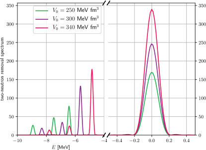
The two-particle spectral function for ²¹⁰Pb is displayed in Figure 11. The peaks are associated with the ground state ($E=0$) as well as with the different excited states. The two peaks closest to $E=0$ correspond to the split-off singlet excitations from Figure 9. We observe that an increase of the pairing strength results in an increase of spectral weight for the lower singlet and the ground state, but in a reduction for all higher eigenstates. The spectral weight ratio between the ground state and the lowest two excitations for $V_{0}=340~{}\text{MeV}~{}\text{fm}^{3}$ is about 14:7:1. Thus, the larger experimental cross section of the state at $E-E_{0}=4.868~{}\text{MeV}$ is not quantitatively reproduced in this simple model. Qualitatively, however, we see that only the two states that are split off from the quasi-continuum (Figure 9) have an appreciable spectral weight at all.

IX Coupling to finite angular momentum

As a final point, we demonstrate that the DMRG is also capable of effectively treating Hamiltonians that are more general than the pure singlet pairing in Equation (2) and investigate model (3). The matrix elements $G^{J}_{jj^{\prime}}$ are independent of $M$ and are again evaluated using the simple contact interaction,

$$G^{J}_{jj^{\prime}}=V^{J}_{0}~{}\big{<}jj;JM\vphantom{\delta^{\left(3\right)}\left(\mathbf{r}_{1}-\mathbf{r}_{2}\right)j^{\prime}j^{\prime};JM}\big{|}\delta^{\left(3\right)}\left(\mathbf{r}_{1}-\mathbf{r}_{2}\right)\big{|}j^{\prime}j^{\prime};JM\vphantom{jj;JM\delta^{\left(3\right)}\left(\mathbf{r}_{1}-\mathbf{r}_{2}\right)}\big{>},$$ (19)

which is reasonable for low to moderate nucleon fillings [72, 82, 85, 80].

The MPO bond dimension is now significantly larger than before due to the presence of many long-range terms. Restricting ourselves to the $N=82-126$ ($N=126-184$) major shell of Pb, the MPO can be compressed down to $\chi_{\text{MPO}}=166$ ($\chi_{\text{MPO}}=234$). Testing the code on the worst case scenario of half-filled ¹⁸⁶Pb [58], we are still able to converge the ground-state wavefunction to a variance per particle of around $10^{-5}\text{MeV}^{2}$ with a couple of hours runtime per eigenstate.

For singlet pairing, it was sufficient to exploit particle number conservation only. At this point, we exploit the conservation of the angular momentum projection $J^{z}$ as well. For every multiplet with integer $J=0,2,4,6,8$ (each containing $2J+1$ states), there is now exactly one state that lies in the sector with $\big{<}J^{z}\big{>}=0$. We can determine $J$ by directly computing $\big{<}\mathbf{J}^{2}\big{>}=J\left(J+1\right)$.

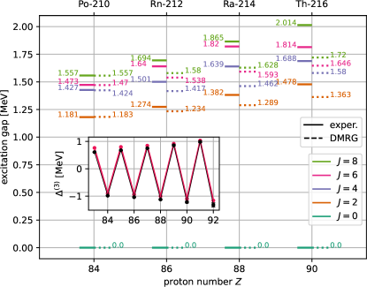
A textbook case are the proton excitations of ²¹⁰Po, which form a sequence with total angular momenta of $J=2,4,6,8$. We extend this analysis to higher isotones by continuing to fill the proton levels up to ²¹⁶Th. In contrast to the literature, we do not only fill the lowest $1h_{9/2}$ level but take into account the full space made up of $1h_{9/2}$, $2f_{7/2}$, $1i_{13/2}$, $2f_{5/2}$, and $3p_{3/2}$ ($L=21$). For these moderate proton fillings, the variance per particle is around $10^{-8}\text{MeV}^{2}$ or less, and the runtime is of the order of tens of minutes.

It is well-known that the delta force interaction alone underpredicts the splitting of the excited state energies [82]. We thus weigh the matrix elements in Equation (19) with different $J$-dependent prefactors $V_{0}^{J}$ (we choose a constant $V_{0}^{J\geq 8}$). $V_{0}^{J=0}$ is determined by fitting the even-odd mass differences of the pure singlet pairing Hamiltonian (2) to the experimental data as before, while the remaining parameters are fitted to the measured splitting of the four lowest eigenenergies of ²¹⁰Po. We obtain, in units of $\text{MeV}~{}\text{fm}^{3}$, $V_{0}^{J=0}=320$, $V_{0}^{J=2}=360$, $V_{0}^{J=4}=230$, $V_{0}^{J=6}=220$, and $V_{0}^{J\geq 8}=-210$.

Figure 11: Two-neutron removal spectral function (18), calculated using the DMRG for ²¹⁰Pb for various pairing strengths at a resolution of $\delta E\approx 0.1~{}\text{MeV}$.

The spectra of the higher isotones up to ²¹⁶Th are shown in Figure 12 (the inset displays the even-odd mass differences used to determine $V_{0}^{J=0}$). While the increase of the energies relative to the ground state is captured qualitatively, the splitting is underestimated quantitatively and clearly requires using a better effective interaction [80, 36].

Figure 12: Excitation energies of the $N=126$ isotones above $Z=82$ calculated with the Hamiltonian (3) that goes beyond singlet pairing. The solid and dotted lines are experimental values and DMRG results, respectively. The inset shows the even-odd mass differences up to ²¹⁸U for $V_{0}^{J=0}=320~{}\text{MeV}~{}\text{fm}^{3}$ (red) in comparison with the experimental values (black) [88].

X Conclusion and outlook

The density-matrix renormalization is very suitable to study simplified nuclear shell models. We argue that the DMRG method should supersede the mean-field BCS approach, as it only brings advantages across the board. We have shown that it is equally effective in dealing with generalized models that have level-dependent matrix elements and additional coupling terms. One can obtain very accurate results – basically up to machine precision – with modest numerical effort even for a very large number of shells. The reason for the efficiency is the naturally low entanglement in the Woods-Saxon basis.

We have demonstrated the capabilities of the method by calculating the even-odd mass differences for all known isotopes of Pb. The energies of the 13 shells were determined from the single-particle Hamiltonian with a Woods-Saxon potential in the Seminole parametrization. Pairing was included via a delta-force interaction whose strength $V_{0}$ is the only free parameter of the calculation. We found that experimental results can be reproduced quantitatively by choosing a universal value of $V_{0}=250~{}\text{MeV}~{}\text{fm}^{3}$ across all neutron fillings.

The DMRG is not just limited to the ground state, but allows one to access excited-state properties as well. To illustrate this, we have computed the low-energy eigenvalue spectrum of the pairing Hamiltonian as well as the two-neutron removal spectral function, which automatically yields the spectral weight for all eigenstates. We found qualitative agreement with the experimental data for the singlet excitations of ²⁰⁸Pb; this can in principle be improved by using a more general Hamiltonian and a better theory of the neutron removal process.

One can readily envision a further extension by continuing to add terms to the Hamiltonian that are most relevant for particular effects, as we did with $J>0$ pairing. Proton-neutron interactions can be incorporated by including the isospin as an additional quantum number. If one goes away from the magic shells, deformation starts to play a role, but it only enters on the one-particle level (e.g., as a deformed Woods-Saxon potential) and can thus be accounted for easily. Studying finite temperatures, which relates to nuclear thermometry [45, 81], would be possible within the grand-canonical ensemble by doubling the system [31, 76, 44, 46].

In terms of further algorithmic development, we may think about more optimal arrangements of orbitals along the chain [84], using a more general tensor network geometry to better account for both neutron and proton states, or exploiting the full rotational symmetry of spherical nuclei. In the latter case, each $j$-level would be a site with an SU(2)-invariant basis. This greatly shrinks the MPO bond dimension but dramatically increases the size of the local basis (up to $D=847$ for $j=13/2$), a problem that also arises for the spatial point-group SU(2) symmetry of molecules and lattices. This idea leads to the question of whether the local basis can be further optimized [50], and the nuclear many-body problem could serve as a testing ground for such methods [50, 47].

Appendix A One-particle parameters

To leading order, the fermions within a nucleus can be described by the single-particle Schrödinger equation with an effective potential. The Woods-Saxon potential [93] is a well-established choice for an undeformed nucleus with spherical symmetry. It is near-constant within the nucleus and has a diffuse boundary, which can be described by a formfactor which is identical to the Fermi function:

$$f_{R,a}\left(r\right)=\frac{1}{\exp\left(\frac{r-R}{a}\right)+1},$$ (20)

where $a$ is the diffuseness of the surface and $R=R_{0}A^{1/3}$ is the nuclear radius. In the Seminole parametrization [77], the effective single-particle Hamiltonian reads:

$$\begin{split}H&=-\frac{\hbar^{2}}{2\mu}\Delta+U^{c}_{R}\left(r\right)-U_{0}~{}g_{N,Z,\kappa}~{}f_{R,a}\left(r\right)\\ &~{}~{}~{}+\lambda\frac{U_{0}\hbar^{2}}{2\mu^{2}c^{2}r}\left(\frac{\partial f_{R_{\text{SO}},a_{\text{SO}}}\left(r\right)}{\partial r}\right)\mathbf{l}\cdot\mathbf{s},\end{split}$$ (21)

with $\mu$ being the reduced mass, $c$ the speed of light, $U^{c}_{R}\left(r\right)$ a Coulomb term which appears for protons only, $g_{N,Z,\kappa}$ an isospin-dependent prefactor ($N$: number of neutrons, $Z$: number of protons, $A=N+Z$), and $\mathbf{l}\cdot\mathbf{s}$ the spin-orbit coupling. The six parameters of the model are given by the potential depth $U_{0}=52.06~{}\text{MeV}$, isospin splitting $\kappa=0.639$, nuclear radius $R_{0}=1.260~{}\text{fm}$, diffuseness $a=a_{\text{SO}}=0.662~{}\text{fm}$, dimensionless spin-orbit coupling $\lambda=24.1$, and spin-orbit radius $R_{0,\text{SO}}=1.16~{}\text{fm}$. The reader is referred to Ref. [77] for more details and a comparison to other parametrizations.

The eigenstates of the single-particle Schrödinger equation are given by

$$\psi_{nljm}\left(r,\theta,\phi\right)=R_{nlj}\left(r\right)i^{l}\mathcal{Y}_{jl}^{m}\left(\theta,\phi\right),$$ (22)

where $m=m_{j}$ is the projection of the total angular momentum $j$ on the z-axis, and $j$ is restricted by the relation $j=l\pm 1/2$ as a result of the action of the spin-orbit operator:

$$\mathbf{l}\cdot\mathbf{s}~{}\psi_{nljm}=\left\{\begin{array}[]{ll}\frac{1}{2}l\psi_{nljm}&j=l+1/2,\\ -\frac{1}{2}\left(l+1\right)\psi_{nljm}&j=l-1/2.\end{array}\right.$$ (23)

$R_{nlj}\left(r\right)$ is the solution of the radial Schrödinger equation, which we obtain numerically using a Chebyshev polynomial technique [94]. $\mathcal{Y}_{jl}^{m}\left(\theta,\phi\right)$ are the spinor spherical harmonics that result from the coupling of the fermionic spin $s=1/2$ to the orbital momentum $l$:

$$\mathcal{Y}_{j=l\pm 1/2}^{m}\left(\theta,\phi\right)=\begin{pmatrix}\alpha^{\uparrow}_{l,m,\pm}~{}Y_{l}^{m-1/2}\left(\theta,\phi\right)\\ \alpha^{\downarrow}_{l,m,\pm}~{}Y_{l}^{m+1/2}\left(\theta,\phi\right)\end{pmatrix},$$ (24)

where $\alpha^{\uparrow}_{l,m,\pm}=\pm\sqrt{\frac{l\pm m+1/2}{2l+1}}$ and $\alpha^{\downarrow}_{l,m,\pm}=\sqrt{\frac{l\mp m+1/2}{2l+1}}$ are the Clebsch-Gordan coefficients of this coupling, only the plus sign is possible for $l=0$; and $Y^{m}_{l}\left(\theta,\phi\right)$ are the regular spherical harmonics (set to $Y^{m}_{l}=0$ for $m>l$). The factor $i^{l}$ is a matter of convention, and is related to time-reversal [42, 12, 72]. As is common practice, we subsume the indices $n$, $l$ and $j$ under one index $j\equiv\left(n,l,j\right)$, which is understood to run over all split levels that are degenerate in $m$, resulting in a shorthand $\big{|}jm\big{>}$ braket notation.

A normalized two-particle state which involves the shells $j_{1}$ and $j_{2}$ and in which the two particles are coupled to a total angular momentum $J$ with a projection $M$ takes the form [85]

$$\big{|}j_{1}j_{2};JM\big{>}=\frac{1}{\sqrt{2}}\sum_{m_{1}m_{2}}C^{JM}_{j_{1}m_{1}j_{2}m_{2}}a^{\dagger}_{j_{1}m_{1}}a^{\dagger}_{j_{2}m_{2}}\big{|}0\big{>},$$ (25)

where $a^{\dagger}_{jm}$ is a fermionic creation operator, and $\big{|}0\big{>}$ denotes the vacuum. For the ground state, the dominant residual interaction term is given by singlet coupling $J=M=0$ in the same $j$-shell, which we can explicitly write out as [95, 85, 53]

$$\begin{split}\big{|}jj;00\big{>}&=\frac{1}{\sqrt{2}}\sum_{m=-j}^{j}\frac{\left(-1\right)^{j-m}}{\sqrt{2j+1}}a^{\dagger}_{j,+m}a^{\dagger}_{j,-m}\big{|}0\big{>}\\ &=\frac{1}{\sqrt{j+\frac{1}{2}}}\sum_{m>0}\left(-1\right)^{j-m}a^{\dagger}_{j,+m}a^{\dagger}_{j,-m}\big{|}0\big{>}.\end{split}$$ (26)

The second-quantized Hamiltonian that describes hoppings of singlet pairs between all $j$-shells with the strengths $G_{jj^{\prime}}$ takes the form of Equation (2):

$$\begin{split}H=\sum_{j,m>0}\epsilon_{j}n_{jm}-&\sum_{jj^{\prime}}G_{jj^{\prime}}\sum_{m>0}\left(-1\right)^{j-m}a^{\dagger}_{jm}a^{\dagger}_{j,-m}\\ \times&\sum_{m^{\prime}>0}\left(-1\right)^{j^{\prime}-m^{\prime}}a_{j^{\prime},-m^{\prime}}a_{j^{\prime}m^{\prime}}.\end{split}$$ (27)

The couplings $G_{jj^{\prime}}$ are a priori unknown. One should note that in order to properly describe excited states, it is necessary to add further quartic terms to the Hamiltonian (see Sec. IX).

Appendix B Dealing with convergence problems

The pairing Hamiltonian Equation (27) has the peculiarity that for odd particle numbers, a unpaired one remains ‘without a partner’ and is unaffected by the pair hopping, thus blocking a particular, a priori unknown orbital. Within exact diagonalization, this can be exploited in the ‘seniority scheme’ to block-diagonalize the Hamiltonian for all possible values of the seniority $s_{j}$, which is essentially the number of unpaired particles in the $j$-shell [53].

Like any numerical variational approach, the DMRG algorithm is prone to getting stuck in states which are not eigenstates (signalled by a large variance Equation (14)) or not the true ground state. In our case, a single particle that gets stuck in an orbital causes the DMRG algorithm to converge to a pair-broken excited eigenstate. Exploiting as few quantum numbers as possible (in this case only the particle number) increases the local fluctuations, which partly improves convergence but does not fully resolve the issue. This problem can be solved for even fillings where we can safely remove the singly occupied states from the local basis and work only with $\big{|}\Downarrow\big{>}_{jm}$ and $\big{|}\Uparrow\big{>}_{jm}$ at each site (which is equivalent to a pseudospin representation).

In order to resolve this issue for odd fillings, we take the full local basis in a given $j$-shell and the restricted basis $\big{|}\Downarrow\big{>}_{jm},\big{|}\Uparrow\big{>}_{jm}$ everywhere else; and compute the lowest state for this configuration. The true ground state is given by the one with the lowest energy among all selections of $j$. Still, we find that this procedure tends to get stuck with a large variance Equation (14). A simple way to help the algorithm is to first determine the ground state $\big{|}E_{0}(N)\big{>}$ for even fillings $N$ and to subsequently use $\sum_{m}a^{\dagger}_{jm}\big{|}E_{0}(N,\text{even})\big{>}$ as initial guesses for odd fillings. These states are already very close to eigenstates, and the remaining convergence is very quick.

An alternative approach to prevent the variational algorithm from getting stuck is to perturb the Hamiltonian, $H\to H+\alpha H_{p}$, where the perturbation $H_{p}$ should contain hopping terms of the type $a^{\dagger}_{jm}a_{j^{\prime}m^{\prime}}$ that make single particles mobile. By slowly letting $\alpha$ go to zero every few iterations, good convergence can be achieved for even fillings. The calculation for odd filling is then performed analogously by using $\sum_{m}a^{\dagger}_{jm}\big{|}E_{0}(N,\text{even})\big{>}$ as an initial guess. This alternative method does not rely on restricting the local basis, which is beneficial if the full wavefunction is needed in subsequent steps. We have tested that both of our approaches yield the same ground state.

We note that the issue does not appear when dealing with the Hamiltonian Equation (3), where more ‘shake-up’ terms are naturally present.

References

- Alford et al. [1983] W. P. Alford, R. N. Boyd, E. Sugarbaker, F. W. N. de Boer, Ronald E. Brown, and E. R. Flynn. Two-step contributions in the two-neutron transfer reaction. Phys. Rev. C, 27:1032–1039, Mar 1983. doi: 10.1103/PhysRevC.27.1032. URL https://link.aps.org/doi/10.1103/PhysRevC.27.1032.
- Alhassid et al. [2008] Y. Alhassid, L. Fang, and H. Nakada. Heavy deformed nuclei in the shell model monte carlo method. Phys. Rev. Lett., 101:082501, Aug 2008. doi: 10.1103/PhysRevLett.101.082501. URL https://link.aps.org/doi/10.1103/PhysRevLett.101.082501.
- Alhassid et al. [2012] Y Alhassid, A Mukherjee, H Nakada, and C Özen. Recent developments in the shell model monte carlo approach to nuclei. Journal of Physics: Conference Series, 403:012012, dec 2012. doi: 10.1088/1742-6596/403/1/012012. URL https://doi.org/10.1088/1742-6596/403/1/012012.
- Amir-Azimi-Nili et al. [1997] K. Amir-Azimi-Nili, J.M. Udias, H. Müther, L.D. Skouras, and A. Polls. Correlations and the cross section of exclusive (e, e’p) reactions for o. Nuclear Physics A, 625(3):633–650, 1997. ISSN 0375-9474. doi: https://doi.org/10.1016/S0375-9474(97)00595-2. URL https://www.sciencedirect.com/science/article/pii/S0375947497005952.
- Anderson [1958] P. W. Anderson. Random-phase approximation in the theory of superconductivity. Phys. Rev., 112:1900–1916, Dec 1958. doi: 10.1103/PhysRev.112.1900. URL https://link.aps.org/doi/10.1103/PhysRev.112.1900.
- Armstrong et al. [2012] J. R. Armstrong, S. Åberg, S. M. Reimann, and V. G. Zelevinsky. Complexity of quantum states in the two-dimensional pairing model. Phys. Rev. E, 86:066204, Dec 2012. doi: 10.1103/PhysRevE.86.066204. URL https://link.aps.org/doi/10.1103/PhysRevE.86.066204.
- Bardeen et al. [1957] J. Bardeen, L. N. Cooper, and J. R. Schrieffer. Theory of superconductivity. Phys. Rev., 108:1175–1204, Dec 1957. doi: 10.1103/PhysRev.108.1175. URL https://link.aps.org/doi/10.1103/PhysRev.108.1175.
- Bayman [1960] B.F. Bayman. A derivation of the pairing-correlation method. Nuclear Physics, 15:33–38, 1960. ISSN 0029-5582. doi: https://doi.org/10.1016/0029-5582(60)90279-0. URL https://www.sciencedirect.com/science/article/pii/0029558260902790.
- Bender et al. [2000] M. Bender, K. Rutz, P.-G. Reinhard, and J. A. Maruhn. Pairing gaps from nuclear mean-field models. The European Physical Journal A, 8(1):59–75, Jul 2000. ISSN 1434-601X. doi: 10.1007/s10050-000-4504-z. URL https://doi.org/10.1007/s10050-000-4504-z.
- Bertsch et al. [2009] G. F. Bertsch, C. A. Bertulani, W. Nazarewicz, N. Schunck, and M. V. Stoitsov. Odd-even mass differences from self-consistent mean field theory. Phys. Rev. C, 79:034306, Mar 2009. doi: 10.1103/PhysRevC.79.034306. URL https://link.aps.org/doi/10.1103/PhysRevC.79.034306.
- Bethe [1931] Hans Bethe. Zur Theorie der Metalle. Zeitschrift für Physik, 71(3-4):205–226, 1931.
- Bohr and Mottelson [1998] Aage Bohr and Ben R Mottelson. Nuclear structure, volume 1. World Scientific, 1998.
- Brink and Broglia [2005] David M Brink and Ricardo A Broglia. Nuclear Superfluidity: pairing in finite systems, volume 24. Cambridge University Press, 2005.
- Broglia and Zelevinsky [2013] Ricardo A Broglia and Vladimir Zelevinsky. Fifty years of nuclear BCS: Pairing in finite systems. World Scientific, 2013.
- Burglin and Rowley [1997] Olivier Burglin and Neil Rowley. Details of nuclear masses away from stability: pairing and deformation effects. Acta Physica Hungarica New Series Heavy Ion Physics, 6(1):189–199, 1997.
- Cerf and Martin [1993] Nicolas Cerf and Olivier Martin. Pairing hamiltonian by a path integral monte carlo procedure. Phys. Rev. C, 47:2610–2615, Jun 1993. doi: 10.1103/PhysRevC.47.2610. URL https://link.aps.org/doi/10.1103/PhysRevC.47.2610.
- Claeys [2018] Pieter W. Claeys. Richardson-Gaudin models and broken integrability, 2018.
- Claeys et al. [2017] Pieter W. Claeys, Jean-Sébastien Caux, Dimitri Van Neck, and Stijn De Baerdemacker. Variational method for integrability-breaking Richardson-Gaudin models. Phys. Rev. B, 96:155149, Oct 2017. doi: 10.1103/PhysRevB.96.155149. URL https://link.aps.org/doi/10.1103/PhysRevB.96.155149.
- Dobaczewski et al. [1995] J Dobaczewski, W Nazarewicz, and T R Werner. Closed shells at drip-line nuclei. Physica Scripta, T56:15–22, jan 1995. doi: 10.1088/0031-8949/1995/t56/002. URL https://doi.org/10.1088/0031-8949/1995/t56/002.
- Dobaczewski et al. [1996] J. Dobaczewski, W. Nazarewicz, T. R. Werner, J. F. Berger, C. R. Chinn, and J. Dechargé. Mean-field description of ground-state properties of drip-line nuclei: Pairing and continuum effects. Phys. Rev. C, 53:2809–2840, Jun 1996. doi: 10.1103/PhysRevC.53.2809. URL https://link.aps.org/doi/10.1103/PhysRevC.53.2809.
- Dukelsky [2014] J Dukelsky. Exactly solvable pairing models in nuclear and mesoscopic physics. Journal of Physics: Conference Series, 533:012057, sep 2014. doi: 10.1088/1742-6596/533/1/012057. URL https://doi.org/10.1088/1742-6596/533/1/012057.
- Dukelsky and Dussel [1999] J. Dukelsky and G. G. Dussel. Application of the density matrix renormalization group to the two level pairing model. Phys. Rev. C, 59:R3005–R3008, Jun 1999. doi: 10.1103/PhysRevC.59.R3005. URL https://link.aps.org/doi/10.1103/PhysRevC.59.R3005.
- Dukelsky and Pittel [2001] J. Dukelsky and S. Pittel. New approach to large-scale nuclear structure calculations. Phys. Rev. C, 63:061303, May 2001. doi: 10.1103/PhysRevC.63.061303. URL https://link.aps.org/doi/10.1103/PhysRevC.63.061303.
- Dukelsky and Sierra [1999] J. Dukelsky and G. Sierra. Density matrix renormalization group study of ultrasmall superconducting grains. Phys. Rev. Lett., 83:172–175, Jul 1999. doi: 10.1103/PhysRevLett.83.172. URL https://link.aps.org/doi/10.1103/PhysRevLett.83.172.
- Dukelsky and Sierra [2000] J. Dukelsky and G. Sierra. Crossover from bulk to few-electron limit in ultrasmall metallic grains. Phys. Rev. B, 61:12302–12314, May 2000. doi: 10.1103/PhysRevB.61.12302. URL https://link.aps.org/doi/10.1103/PhysRevB.61.12302.
- Dukelsky et al. [2002] J. Dukelsky, S. Pittel, S. S. Dimitrova, and M. V. Stoitsov. Density matrix renormalization group method and large-scale nuclear shell-model calculations. Phys. Rev. C, 65:054319, May 2002. doi: 10.1103/PhysRevC.65.054319. URL https://link.aps.org/doi/10.1103/PhysRevC.65.054319.
- Dukelsky et al. [2004] J. Dukelsky, S. Pittel, and G. Sierra. Colloquium: Exactly solvable Richardson-Gaudin models for many-body quantum systems. Rev. Mod. Phys., 76:643–662, Aug 2004. doi: 10.1103/RevModPhys.76.643. URL https://link.aps.org/doi/10.1103/RevModPhys.76.643.
- Dukelsky et al. [2011] J. Dukelsky, S. Lerma H., L. M. Robledo, R. Rodriguez-Guzman, and S. M. A. Rombouts. Exactly solvable pairing Hamiltonian for heavy nuclei. Phys. Rev. C, 84:061301(R), Dec 2011. doi: 10.1103/PhysRevC.84.061301. URL https://link.aps.org/doi/10.1103/PhysRevC.84.061301.
- Dukelsky and Pittel [2013] Jorge Dukelsky and S Pittel. Exact solutions for pairing interactions. In Fifty Years of Nuclear BCS: Pairing in Finite Systems, pages 200–211. World Scientific, 2013.
- Eisert et al. [2010] J. Eisert, M. Cramer, and M. B. Plenio. Colloquium: Area laws for the entanglement entropy. Rev. Mod. Phys., 82:277–306, Feb 2010. doi: 10.1103/RevModPhys.82.277. URL https://link.aps.org/doi/10.1103/RevModPhys.82.277.
- Feiguin and White [2005] Adrian E. Feiguin and Steven R. White. Finite-temperature density matrix renormalization using an enlarged Hilbert space. Phys. Rev. B, 72:220401(R), Dec 2005. doi: 10.1103/PhysRevB.72.220401. URL https://link.aps.org/doi/10.1103/PhysRevB.72.220401.
- Fukuda [2010] Y. Fukuda. Appearance potential spectroscopy (APS): Old method, but applicable to study of nano-structures. Analytical Sciences, 26(2):187–197, 2010. doi: 10.2116/analsci.26.187.
- Geurts et al. [1996] W. J. W. Geurts, K. Allaart, W. H. Dickhoff, and H. Müther. Two-nucleon spectral function of at high momenta. Phys. Rev. C, 54:1144–1157, Sep 1996. doi: 10.1103/PhysRevC.54.1144. URL https://link.aps.org/doi/10.1103/PhysRevC.54.1144.
- Gobert et al. [2004a] D. Gobert, U. Schollwöck, and J. von Delft. Josephson effect between superconducting nanograins with discrete energy levels. The European Physical Journal B - Condensed Matter and Complex Systems, 38(3):501–513, Apr 2004a. ISSN 1434-6036. doi: 10.1140/epjb/e2004-00145-6. URL https://doi.org/10.1140/epjb/e2004-00145-6.
- Gobert et al. [2004b] Dominique Gobert, Moshe Schechter, Ulrich Schollwöck, and Jan von Delft. Well-defined quasiparticles in interacting metallic grains. Phys. Rev. Lett., 93:186402, Oct 2004b. doi: 10.1103/PhysRevLett.93.186402. URL https://link.aps.org/doi/10.1103/PhysRevLett.93.186402.
- Gottardo et al. [2012] A. Gottardo, J. J. Valiente-Dobón, G. Benzoni, R. Nicolini, A. Gadea, S. Lunardi, P. Boutachkov, A. M. Bruce, M. Górska, J. Grebosz, S. Pietri, Zs. Podolyák, M. Pfützner, P. H. Regan, H. Weick, J. Alcántara Núñez, A. Algora, N. Al-Dahan, G. de Angelis, Y. Ayyad, N. Alkhomashi, P. R. P. Allegro, D. Bazzacco, J. Benlliure, M. Bowry, A. Bracco, M. Bunce, F. Camera, E. Casarejos, M. L. Cortes, F. C. L. Crespi, A. Corsi, A. M. Denis Bacelar, A. Y. Deo, C. Domingo-Pardo, M. Doncel, Zs. Dombradi, T. Engert, K. Eppinger, G. F. Farrelly, F. Farinon, E. Farnea, H. Geissel, J. Gerl, N. Goel, E. Gregor, T. Habermann, R. Hoischen, R. Janik, S. Klupp, I. Kojouharov, N. Kurz, S. M. Lenzi, S. Leoni, S. Mandal, R. Menegazzo, D. Mengoni, B. Million, A. I. Morales, D. R. Napoli, F. Naqvi, C. Nociforo, A. Prochazka, W. Prokopowicz, F. Recchia, R. V. Ribas, M. W. Reed, D. Rudolph, E. Sahin, H. Schaffner, A. Sharma, B. Sitar, D. Siwal, K. Steiger, P. Strmen, T. P. D. Swan, I. Szarka, C. A. Ur, P. M. Walker, O. Wieland, H-J. Wollersheim, F. Nowacki, E. Maglione, and A. P. Zuker. New isomers in the full seniority scheme of neutron-rich lead isotopes: The role of effective three-body forces. Phys. Rev. Lett., 109:162502, Oct 2012. doi: 10.1103/PhysRevLett.109.162502. URL https://link.aps.org/doi/10.1103/PhysRevLett.109.162502.
- Heyde [1994] KLG Heyde. The nuclear shell model. Study edition. Springer-Verlag, 1994.
- Hjorth-Jensen et al. [2017] Morten Hjorth-Jensen, Maria Paola Lombardo, and Ubirajara Van Kolck. An advanced course in computational nuclear physics. Springer Lecture Notes in Physics, 936, 2017.
- Holt et al. [1998] A. Holt, T. Engeland, M. Hjorth-Jensen, and E. Osnes. Effective interactions and shell model studies of heavy tin isotopes. Nuclear Physics A, 634(1):41–56, 1998. ISSN 0375-9474. doi: https://doi.org/10.1016/S0375-9474(98)00146-8. URL https://www.sciencedirect.com/science/article/pii/S0375947498001468.
- Hubig et al. [2015] C. Hubig, I. P. McCulloch, U. Schollwöck, and F. A. Wolf. Strictly single-site DMRG algorithm with subspace expansion. Phys. Rev. B, 91:155115, Apr 2015. doi: 10.1103/PhysRevB.91.155115. URL https://link.aps.org/doi/10.1103/PhysRevB.91.155115.
- Hubig et al. [2017] C. Hubig, I. P. McCulloch, and U. Schollwöck. Generic construction of efficient matrix product operators. Phys. Rev. B, 95:035129, Jan 2017. doi: 10.1103/PhysRevB.95.035129. URL https://link.aps.org/doi/10.1103/PhysRevB.95.035129.
- Huby [1954] R Huby. Phase of matrix elements in nuclear reactions and radioactive decay. Proceedings of the Physical Society. Section A, 67(12):1103–1105, dec 1954. doi: 10.1088/0370-1298/67/12/408. URL https://doi.org/10.1088/0370-1298/67/12/408.
- Igo et al. [1970] G. J. Igo, P. D. Barnes, and E. R. Flynn. Mixing of two-particle, two-hole states in . Phys. Rev. Lett., 24:470–473, Mar 1970. doi: 10.1103/PhysRevLett.24.470. URL https://link.aps.org/doi/10.1103/PhysRevLett.24.470.
- Karrasch et al. [2012] C. Karrasch, J. H. Bardarson, and J. E. Moore. Finite-temperature dynamical density matrix renormalization group and the Drude weight of spin- chains. Phys. Rev. Lett., 108:227206, May 2012. doi: 10.1103/PhysRevLett.108.227206. URL https://link.aps.org/doi/10.1103/PhysRevLett.108.227206.
- Kelić et al. [2006] A. Kelić, J. B. Natowitz, and K. H. Schmidt. Nuclear thermometry. In Philippe Chomaz, Francesca Gulminelli, Wolfgang Trautmann, and Sherry J. Yennello, editors, Dynamics and Thermodynamics with Nuclear Degrees of Freedom, pages 203–213, Berlin, Heidelberg, 2006. Springer Berlin Heidelberg. ISBN 978-3-540-46496-9.
- Kennes and Karrasch [2016] D.M. Kennes and C. Karrasch. Extending the range of real time density matrix renormalization group simulations. Computer Physics Communications, 200:37 – 43, 2016. ISSN 0010-4655. doi: https://doi.org/10.1016/j.cpc.2015.10.019. URL http://www.sciencedirect.com/science/article/pii/S0010465515004002.
- Köhler et al. [2020] Thomas Köhler, Jan Stolpp, and Sebastian Paeckel. Efficient and flexible approach to simulate low-dimensional quantum lattice models with large local Hilbert spaces. 2020.
- Koonin et al. [1997a] S. E. Koonin, D. J. Dean, and K. Langanke. Results from shell-model monte carlo studies. Annual Review of Nuclear and Particle Science, 47(1):463–504, 1997a. doi: 10.1146/annurev.nucl.47.1.463. URL https://doi.org/10.1146/annurev.nucl.47.1.463.
- Koonin et al. [1997b] S.E. Koonin, D.J. Dean, and K. Langanke. Shell model monte carlo methods. Physics Reports, 278(1):1–77, 1997b. ISSN 0370-1573. doi: https://doi.org/10.1016/S0370-1573(96)00017-8. URL https://www.sciencedirect.com/science/article/pii/S0370157396000178.
- Krumnow et al. [2016] C. Krumnow, L. Veis, Ö. Legeza, and J. Eisert. Fermionic orbital optimization in tensor network states. Phys. Rev. Lett., 117:210402, Nov 2016. doi: 10.1103/PhysRevLett.117.210402. URL https://link.aps.org/doi/10.1103/PhysRevLett.117.210402.
- Legeza et al. [2015] Ö. Legeza, L. Veis, A. Poves, and J. Dukelsky. Advanced density matrix renormalization group method for nuclear structure calculations. Phys. Rev. C, 92:051303, Nov 2015. doi: 10.1103/PhysRevC.92.051303. URL https://link.aps.org/doi/10.1103/PhysRevC.92.051303.
- Lingle and Volya [2015] Mark Lingle and Alexander Volya. Nuclear pairing within a configuration-space monte carlo approach. Phys. Rev. C, 91:064304, Jun 2015. doi: 10.1103/PhysRevC.91.064304. URL https://link.aps.org/doi/10.1103/PhysRevC.91.064304.
- Liu et al. [2020] Xiaoyu Liu, Chong Qi, Xin Guan, and Zhong Liu. PairDiagSph: Generalization of the exact pairing diagonalization program for spherical systems. 2020.
- Molique and Dudek [1997] H. Molique and J. Dudek. Fock-space diagonalization of the state-dependent pairing Hamiltonian with the Woods-Saxon mean field. Phys. Rev. C, 56:1795–1813, Oct 1997. doi: 10.1103/PhysRevC.56.1795. URL https://link.aps.org/doi/10.1103/PhysRevC.56.1795.
- Mukherjee et al. [2011] Abhishek Mukherjee, Y. Alhassid, and G. F. Bertsch. Number-conserving theory of nuclear pairing gaps: A global assessment. Phys. Rev. C, 83:014319, Jan 2011. doi: 10.1103/PhysRevC.83.014319. URL https://link.aps.org/doi/10.1103/PhysRevC.83.014319.
- Müther et al. [1995] H. Müther, A. Polls, and W. H. Dickhoff. Momentum and energy distributions of nucleons in finite nuclei due to short-range correlations. Phys. Rev. C, 51:3040–3051, Jun 1995. doi: 10.1103/PhysRevC.51.3040. URL https://link.aps.org/doi/10.1103/PhysRevC.51.3040.
- Nakada and Alhassid [1997] H. Nakada and Y. Alhassid. Total and parity-projected level densities of iron-region nuclei in the auxiliary fields monte carlo shell model. Phys. Rev. Lett., 79:2939–2942, Oct 1997. doi: 10.1103/PhysRevLett.79.2939. URL https://link.aps.org/doi/10.1103/PhysRevLett.79.2939.
- Pakarinen et al. [2007] J. Pakarinen, V. Hellemans, R. Julin, S. Juutinen, K. Heyde, P.-H. Heenen, M. Bender, I. G. Darby, S. Eeckhaudt, T. Enqvist, T. Grahn, P. T. Greenlees, F. Johnston-Theasby, P. Jones, H. Kettunen, M. Leino, A.-P. Leppänen, P. Nieminen, M. Nyman, R. D. Page, P. M. Raddon, P. Rahkila, C. Scholey, J. Uusitalo, and R. Wadsworth. Investigation of nuclear collectivity in the neutron mid-shell nucleus . Phys. Rev. C, 75:014302, Jan 2007. doi: 10.1103/PhysRevC.75.014302. URL https://link.aps.org/doi/10.1103/PhysRevC.75.014302.
- Pal and Stamp [1967] M.K. Pal and A.P. Stamp. Pairing effects in nuclei described by the Hartree-Fock theory. Nuclear Physics A, 99(2):228–240, 1967. ISSN 0375-9474. doi: https://doi.org/10.1016/0375-9474(67)90338-7. URL https://www.sciencedirect.com/science/article/pii/0375947467903387.
- Pan et al. [2004] Feng Pan, V. G. Gueorguiev, and J. P. Draayer. Algebraic solutions of an extended pairing model for well deformed nuclei. Phys. Rev. Lett., 92:112503, Mar 2004. doi: 10.1103/PhysRevLett.92.112503. URL https://link.aps.org/doi/10.1103/PhysRevLett.92.112503.
- Pan et al. [2017] Feng Pan, Xin Guan, and Jerry P Draayer. Exactly solvable pairing in a mean-field framework: Models and applications. Emergent Phenomena In Atomic Nuclei From Large-scale Modeling: A Symmetry-guided Perspective, page 327, 2017.
- Papenbrock and Dean [2005] T Papenbrock and D J Dean. Density matrix renormalization group and wavefunction factorization for nuclei. Journal of Physics G: Nuclear and Particle Physics, 31(8):S1377, jul 2005. doi: 10.1088/0954-3899/31/8/016. URL https://dx.doi.org/10.1088/0954-3899/31/8/016.
- Pavešić et al. [2021] Luka Pavešić, Daniel Bauernfeind, and Rok Žitko. Subgap states in superconducting islands. Phys. Rev. B, 104:L241409, Dec 2021. doi: 10.1103/PhysRevB.104.L241409. URL https://link.aps.org/doi/10.1103/PhysRevB.104.L241409.
- Pieper and Wiringa [2001] Steven C. Pieper and R. B. Wiringa. Quantum monte carlo calculations of light nuclei. Annual Review of Nuclear and Particle Science, 51(1):53–90, 2001. doi: 10.1146/annurev.nucl.51.101701.132506. URL https://doi.org/10.1146/annurev.nucl.51.101701.132506.
- Pirvu et al. [2010] B Pirvu, V Murg, J I Cirac, and F Verstraete. Matrix product operator representations. New Journal of Physics, 12(2):025012, feb 2010. doi: 10.1088/1367-2630/12/2/025012. URL https://dx.doi.org/10.1088/1367-2630/12/2/025012.
- Pittel [2015] S Pittel. Recent advances in exact solutions of pairing models. Journal of Physics: Conference Series, 578:012011, jan 2015. doi: 10.1088/1742-6596/578/1/012011. URL https://doi.org/10.1088/1742-6596/578/1/012011.
- Pittel and Sandulescu [2006] S. Pittel and N. Sandulescu. Density matrix renormalization group and the nuclear shell model. Phys. Rev. C, 73:014301, Jan 2006. doi: 10.1103/PhysRevC.73.014301. URL https://link.aps.org/doi/10.1103/PhysRevC.73.014301.
- Potthoff et al. [1993] M. Potthoff, J. Braun, G. Borstel, and W. Nolting. Theory of Auger electron and appearance-potential spectroscopy from solids with partially filled valence bands: Effects of valence-band–core interaction. Phys. Rev. B, 47:12480–12497, May 1993. doi: 10.1103/PhysRevB.47.12480. URL https://link.aps.org/doi/10.1103/PhysRevB.47.12480.
- Qi et al. [2016] Chong Qi, L. Y. Jia, and G. J. Fu. Large-scale shell-model calculations on the spectroscopy of pb isotopes. Phys. Rev. C, 94:014312, Jul 2016. doi: 10.1103/PhysRevC.94.014312. URL https://link.aps.org/doi/10.1103/PhysRevC.94.014312.
- Rausch and Potthoff [2016] Roman Rausch and Michael Potthoff. Multiplons in the two-hole excitation spectra of the one-dimensional Hubbard model. New Journal of Physics, 18(2):023033, feb 2016. doi: 10.1088/1367-2630/18/2/023033. URL https://doi.org/10.1088/1367-2630/18/2/023033.
- Richardson [1966] R. W. Richardson. Numerical study of the 8-32-particle eigenstates of the pairing Hamiltonian. Phys. Rev., 141:949–956, Jan 1966. doi: 10.1103/PhysRev.141.949. URL https://link.aps.org/doi/10.1103/PhysRev.141.949.
- Rowe and Wood [2010] David J Rowe and John L Wood. Fundamentals of nuclear models: Foundational models. World Scientific, 2010.
- Sambataro [2012] M. Sambataro. Multipair approach to pairing in nuclei. Phys. Rev. C, 85:064326, Jun 2012. doi: 10.1103/PhysRevC.85.064326. URL https://link.aps.org/doi/10.1103/PhysRevC.85.064326.
- Sandulescu and Bertsch [2008] N. Sandulescu and G. F. Bertsch. Accuracy of BCS-based approximations for pairing in small fermi systems. Phys. Rev. C, 78:064318, Dec 2008. doi: 10.1103/PhysRevC.78.064318. URL https://link.aps.org/doi/10.1103/PhysRevC.78.064318.
- Schollwöck [2005] U. Schollwöck. The density-matrix renormalization group. Rev. Mod. Phys., 77:259–315, Apr 2005. doi: 10.1103/RevModPhys.77.259. URL https://link.aps.org/doi/10.1103/RevModPhys.77.259.
- Schollwöck [2011] Ulrich Schollwöck. The density-matrix renormalization group in the age of matrix product states. Annals of Physics, 326(1):96–192, 2011. ISSN 0003-4916. doi: https://doi.org/10.1016/j.aop.2010.09.012. URL https://www.sciencedirect.com/science/article/pii/S0003491610001752. January 2011 Special Issue.
- Schwierz et al. [2007] N. Schwierz, I. Wiedenhover, and A. Volya. Parameterization of the Woods-Saxon potential for shell-model calculations. 2007.
- Silver et al. [1996] R.N. Silver, H. Roeder, A.F. Voter, and J.D. Kress. Kernel polynomial approximations for densities of states and spectral functions. Journal of Computational Physics, 124(1):115–130, 1996. ISSN 0021-9991. doi: https://doi.org/10.1006/jcph.1996.0048. URL https://www.sciencedirect.com/science/article/pii/S0021999196900480.
- [79] Alejandro A. Sonzogni. National nuclear data center, information extracted from the NuDat 2 database. URL https://www.nndc.bnl.gov/nudat2/.
- Stepanov, M. et al. [2018] Stepanov, M., Imasheva, L., Ishkhanov, B., and Tretyakova, T. Pairing and (9/2)n configuration in nuclei in the 208Pb region. EPJ Web Conf., 177:03004, 2018. doi: 10.1051/epjconf/201817703004. URL https://doi.org/10.1051/epjconf/201817703004.
- Sumaryada and Volya [2007] Tony Sumaryada and Alexander Volya. Thermodynamics of pairing in mesoscopic systems. Phys. Rev. C, 76:024319, Aug 2007. doi: 10.1103/PhysRevC.76.024319. URL https://link.aps.org/doi/10.1103/PhysRevC.76.024319.
- Talmi [2017] Igal Talmi. Simple models of complex nuclei. Routledge, 2017.
- Thakur et al. [2008] B. Thakur, S. Pittel, and N. Sandulescu. Density matrix renormalization group study of and . Phys. Rev. C, 78:041303, Oct 2008. doi: 10.1103/PhysRevC.78.041303. URL https://link.aps.org/doi/10.1103/PhysRevC.78.041303.
- Tichai et al. [2022] A. Tichai, S. Knecht, A. T. Kruppa, Ö. Legeza, C. P. Moca, A. Schwenk, M. A. Werner, and G. Zarand. Combining the in-medium similarity renormalization group with the density matrix renormalization group: Shell structure and information entropy, 2022.
- V. Zelevinsky [2017] A. Volya V. Zelevinsky. Physics of Atomic Nuclei. John Wiley & Sons, Ltd, 2017. ISBN 9783527693610. doi: https://doi.org/10.1002/9783527693610.
- Volya et al. [2001] Alexander Volya, B.Alex Brown, and Vladimir Zelevinsky. Exact solution of the nuclear pairing problem. Physics Letters B, 509(1):37 – 42, 2001. ISSN 0370-2693. doi: https://doi.org/10.1016/S0370-2693(01)00431-2. URL http://www.sciencedirect.com/science/article/pii/S0370269301004312.
- von Delft [2001] Jan von Delft. Superconductivity in ultrasmall metallic grains. Annalen der Physik, 513(3):219–276, 2001. doi: https://doi.org/10.1002/andp.20015130302. URL https://onlinelibrary.wiley.com/doi/abs/10.1002/andp.20015130302.
- Wang et al. [2021] Meng Wang, W.J. Huang, F.G. Kondev, G. Audi, and S. Naimi. The AME 2020 atomic mass evaluation (II). Tables, graphs and references. Chinese Physics C, 45(3):030003, mar 2021. doi: 10.1088/1674-1137/abddaf. URL https://doi.org/10.1088/1674-1137/abddaf.
- Weiße et al. [2006] Alexander Weiße, Gerhard Wellein, Andreas Alvermann, and Holger Fehske. The kernel polynomial method. Rev. Mod. Phys., 78:275–306, Mar 2006. doi: 10.1103/RevModPhys.78.275. URL https://link.aps.org/doi/10.1103/RevModPhys.78.275.
- Weissmann and Müller [1981] R. Weissmann and K. Müller. Auger electron spectroscopy - a local probe for solid surfaces. Surface Science Reports, 1(5):251–309, 1981. ISSN 0167-5729. doi: https://doi.org/10.1016/0167-5729(81)90005-4. URL https://www.sciencedirect.com/science/article/pii/0167572981900054.
- White [1992] Steven R. White. Density matrix formulation for quantum renormalization groups. Phys. Rev. Lett., 69:2863–2866, Nov 1992. doi: 10.1103/PhysRevLett.69.2863. URL https://link.aps.org/doi/10.1103/PhysRevLett.69.2863.
- White et al. [1992] Steven R. White, Sudip Chakravarty, Martin P. Gelfand, and Steven A. Kivelson. Pair binding in small Hubbard-model molecules. Phys. Rev. B, 45:5062–5065, Mar 1992. doi: 10.1103/PhysRevB.45.5062. URL https://link.aps.org/doi/10.1103/PhysRevB.45.5062.
- Woods and Saxon [1954] Roger D. Woods and David S. Saxon. Diffuse surface optical model for nucleon-nuclei scattering. Phys. Rev., 95:577–578, Jul 1954. doi: 10.1103/PhysRev.95.577. URL https://link.aps.org/doi/10.1103/PhysRev.95.577.
- Yücel [2015] Uğur Yücel. Numerical approximations of Sturm–Liouville eigenvalues using Chebyshev polynomial expansions method. Cogent Mathematics, 2(1), 2015. doi: 10.1080/23311835.2015.1045223. URL http://doi.org/10.1080/23311835.2015.1045223.
- Zelevinsky and Volya [2003] Vladimir Zelevinsky and Alexander Volya. Nuclear pairing: New perspectives. Physics of Atomic Nuclei, 66(10):1781–1801, 2003.