Actuarial strategy for pricing Asian options under a mixed fractional Brownian motion with jumps

Foad Shokrollahi Department of Mathematics and Statistics, University of Vaasa, P.O. Box 700, FIN-65101 Vaasa, FINLAND foad.shokrollahi@uva.fi Davood Ahmadian Faculty of Mathematical Sciences, University of Tabriz 29Blvd, Tabriz, Iran d.ahmadian@tabrizu.ac.ir  and  Luca Vincenzo Ballestra Department of Statistical Sciences, Alma Mater Studiorum University of Bologna, Via delle Belle Arti 41, 40126 Bologna, Italy luca.ballestra@unibo.it
(Date: March 18, 2024)
Abstract.

The mixed fractional Brownian motion (mfBm𝑚𝑓𝐵𝑚mfBm) has become quite popular in finance, since it allows one to model long-range dependence and self-similarity while remaining, for certain values of the Hurst parameter, arbitrage-free. In the present paper, we propose approximate closed-form solutions for pricing arithmetic Asian options on an underlying described by the mfBm𝑚𝑓𝐵𝑚mfBm. Specifically, we consider both arithmetic Asian options and arithmetic Asian power options, and we obtain analytical formulas for pricing them based on a convenient approximation of the strike price. Both the standard mfBm𝑚𝑓𝐵𝑚mfBm and the mfBm𝑚𝑓𝐵𝑚mfBm with Poisson log-normally distributed jumps are taken into account.

Key words and phrases:
Mixed fractional Brownian motion; Asian options; Power options; Jump-diffusion; Option pricing
2010 Mathematics Subject Classification:
91G20; 91G80; 60G22

1. Introduction

As documented by several empirical studies, returns of financial assets are often affected by long-range dependence and self-similarity, and thus several scholars have proposed to model them by using the so-called fractional Brownian motion (fBm𝑓𝐵𝑚fBm) with Hurst exponent H(1/2,1)𝐻121H\in(1/2,1), see, e.g., [9], [12], [17]. Nevertheless, as shown in [3], and [7], the fBm𝑓𝐵𝑚fBm is not arbutrage-free, and thus, some authors [6], [13], [14], [28] have proposed to use the so-called mixed fractional Brownian motion (mfBm𝑚𝑓𝐵𝑚mfBm), i.e., a linear combination of the Wiener process and the fBm𝑓𝐵𝑚fBm itself. When the Hurst exponent of the fBm𝑓𝐵𝑚fBm is greater than 1/2121/2, the mfBm𝑚𝑓𝐵𝑚mfBm results in a Gaussian long-memory process suitable for modeling the returns of financial assets. Furthermore, as shown in [6], if H𝐻H is greater than 3/4343/4 the mfBm𝑚𝑓𝐵𝑚mfBm is arbitrage-free. Therefore, the mfBm𝑚𝑓𝐵𝑚mfBm has been largely employed for pricing various kinds of derivatives, including stock options [2], [5], [25], equity warrants [26], currency options [22, 20, 19], and credit derivatives [10].

The mfBm𝑚𝑓𝐵𝑚mfBm has also been used for pricing Asian options, i.e. options whose payoff depends on the average, either geometric or arithmetic, of the underlying asset over the whole option’s lifespan [18]. In particular, [16] obtained an exact closed-form solution for geometric Asian options, [27] derived an exact analytical formula for geometric Asian power options, [25] proposed an exact closed-form solution for geometric Asian rainbow options on two underlying assets, which was generalized to the case on an arbitrarily large number of underlying assets in [1]. Furthermore, [15] considered a mfBm𝑚𝑓𝐵𝑚mfBm with jumps and obtained an exact analytical formula for valuing geometric Asian power options.

All the exact closed-form solutions proposed in the aforementioned papers are valid for Asian options of geometric type. By contrast, for arithemtic Asian options, exact closed-form solutions cannot be found, and thus some numerical approximation is required. To this aim, some researchers have proposed to apply the Monte Carlo simulation method, which could also be enhanced by using the price of a geometric Asian option as a control variate (see [15]). Nevertheless, this approach, albeit flexible and relatively simple to implement, has the disadvantage of being very slow to converge.

Therefore, in this paper we propose the use of approximate closed-form solutions. Specifically, we consider both arithmetic Asian options and arithmetic Asian power options, and we value them by applying an analytical formula that we obtain by a convenient approximation of the strike price. Both the standard mfBm𝑚𝑓𝐵𝑚mfBm and the mfBm𝑚𝑓𝐵𝑚mfBm with Poisson log-normally distributed jumps are taken into account.

The remainder of the paper is organized as follows: in Section 2 we describe the mfBm𝑚𝑓𝐵𝑚mfBm with jumps and present exact analytical formulas for pricing Asian options of geometric type. In Section 3 we derive an approximate closed-form solution for pricing arithmetic Asian options, which in Section 4 we extend to arithmetic Asian power options. Finally, Section 5 concludes.

2. Preliminaries

We assume that the following assumptions hold:

  1. (i)

    the dynamics of the stock price is governed by the following equation

    (2.1) St=S0exp{f(t)+σBt+εBtH12σ2t12ε2t2H+i=1NtJi},subscript𝑆𝑡subscript𝑆0𝑓𝑡𝜎subscript𝐵𝑡𝜀superscriptsubscript𝐵𝑡𝐻12superscript𝜎2𝑡12superscript𝜀2superscript𝑡2𝐻superscriptsubscript𝑖1subscript𝑁𝑡subscript𝐽𝑖\displaystyle S_{t}=S_{0}\exp\{f(t)+\sigma B_{t}+\varepsilon B_{t}^{H}-\frac{1}{2}\sigma^{2}t-\frac{1}{2}\varepsilon^{2}t^{2H}+\sum_{i=1}^{N_{t}}J_{i}\},

    where f(t)𝑓𝑡f(t) is a non-random function of t𝑡t, and, σ𝜎\sigma, ε𝜀\varepsilon are constants; Btsubscript𝐵𝑡B_{t} and BtHsuperscriptsubscript𝐵𝑡𝐻B_{t}^{H} are a standard Brownian motion and a fBm𝑓𝐵𝑚fBm respectively; Ntsubscript𝑁𝑡N_{t} is a poisson process with rate λ𝜆\lambda; eJi1superscript𝑒subscript𝐽𝑖1e^{J_{i}}-1 is jump size which is a sequence of independent identically distributed and JiN(μJ,σJ2)similar-tosubscript𝐽𝑖𝑁subscript𝜇𝐽superscriptsubscript𝜎𝐽2J_{i}\sim N(\mu_{J},\sigma_{J}^{2}). Moreover, all three sources of randomness, the Btsubscript𝐵𝑡B_{t} and BtHsuperscriptsubscript𝐵𝑡𝐻B_{t}^{H} and Ntsubscript𝑁𝑡N_{t} are supposed to be independent;

  2. (ii)

    the risk free interest rate r𝑟r and dividend rate q𝑞q are known and constant through time;

  3. (iii)

    the option can be exercised only at the maturity time;

  4. (iv)

    there are no transaction costs in buying or selling the stocks or option.

Based on option valuation strategy and risk neutral measure (cf.Refs.[8, 21]), the dynamics of the stock price process S(t)𝑆𝑡S(t) can be written as:

(2.2) St=S0exp[(rq)t+σBt+εBtH12σ2t12ε2t2H+i=1NtJi].subscript𝑆𝑡subscript𝑆0𝑟𝑞𝑡𝜎subscript𝐵𝑡𝜀superscriptsubscript𝐵𝑡𝐻12superscript𝜎2𝑡12superscript𝜀2superscript𝑡2𝐻superscriptsubscript𝑖1subscript𝑁𝑡subscript𝐽𝑖\displaystyle S_{t}=S_{0}\exp[(r-q)t+\sigma B_{t}+\varepsilon B_{t}^{H}-\frac{1}{2}\sigma^{2}t-\frac{1}{2}\varepsilon^{2}t^{2H}+\sum_{i=1}^{N_{t}}J_{i}].
Lemma 2.1.
(2.3) E[ST]=S0e(rq)T+λ(ρ1)T.𝐸delimited-[]subscript𝑆𝑇subscript𝑆0superscript𝑒𝑟𝑞𝑇𝜆𝜌1𝑇\displaystyle E[S_{T}]=S_{0}e^{(r-q)T+\lambda(\rho-1)T}.

where ρ=E[eJ1]𝜌𝐸delimited-[]superscript𝑒subscript𝐽1\rho=E[e^{J_{1}}].

Proof.
(2.4) E[ST]𝐸delimited-[]subscript𝑆𝑇\displaystyle E[S_{T}] =\displaystyle= S0E[e(rq)t+σBt+εBtH12σ2t12ε2t2H+i=1NTJi\displaystyle S_{0}E[e^{(r-q)t+\sigma B_{t}+\varepsilon B_{t}^{H}-\frac{1}{2}\sigma^{2}t-\frac{1}{2}\varepsilon^{2}t^{2H}+\sum_{i=1}^{N_{T}}J_{i}}
=\displaystyle= S0E[e(rq)t+σBt+εBtH12σ2t12ε2t2H]E[i=1NTeJi]subscript𝑆0𝐸delimited-[]superscript𝑒𝑟𝑞𝑡𝜎subscript𝐵𝑡𝜀superscriptsubscript𝐵𝑡𝐻12superscript𝜎2𝑡12superscript𝜀2superscript𝑡2𝐻𝐸delimited-[]superscriptsubscriptproduct𝑖1subscript𝑁𝑇superscript𝑒subscript𝐽𝑖\displaystyle S_{0}E[e^{(r-q)t+\sigma B_{t}+\varepsilon B_{t}^{H}-\frac{1}{2}\sigma^{2}t-\frac{1}{2}\varepsilon^{2}t^{2H}}]E[\prod_{i=1}^{N_{T}}e^{J_{i}}]
=\displaystyle= S0e(rq)TE[i=0NTeJi],subscript𝑆0superscript𝑒𝑟𝑞𝑇𝐸delimited-[]superscriptsubscriptproduct𝑖0subscript𝑁𝑇superscript𝑒subscript𝐽𝑖\displaystyle S_{0}e^{(r-q)T}E[\prod_{i=0}^{N_{T}}e^{J_{i}}],

and

(2.5) E[i=0NTeJi]𝐸delimited-[]superscriptsubscriptproduct𝑖0subscript𝑁𝑇superscript𝑒subscript𝐽𝑖\displaystyle E\left[\prod_{i=0}^{N_{T}}e^{J_{i}}\right] =\displaystyle= n=0(λT)neλTn!E[i=1neJi]superscriptsubscript𝑛0superscript𝜆𝑇𝑛superscript𝑒𝜆𝑇𝑛𝐸delimited-[]superscriptsubscriptproduct𝑖1𝑛superscript𝑒subscript𝐽𝑖\displaystyle\sum_{n=0}^{\infty}\frac{(\lambda T)^{n}e^{-\lambda T}}{n!}E[\prod_{i=1}^{n}e^{J_{i}}]
=\displaystyle= n=0(λT)neλTn!ρnsuperscriptsubscript𝑛0superscript𝜆𝑇𝑛superscript𝑒𝜆𝑇𝑛superscript𝜌𝑛\displaystyle\sum_{n=0}^{\infty}\frac{(\lambda T)^{n}e^{-\lambda T}}{n!}\rho^{n}
=\displaystyle= eλ(ρ1)Tn=0(λT)neρλTn!superscript𝑒𝜆𝜌1𝑇superscriptsubscript𝑛0superscript𝜆𝑇𝑛superscript𝑒𝜌𝜆𝑇𝑛\displaystyle e^{\lambda(\rho-1)T}\sum_{n=0}^{\infty}\frac{(\lambda T)^{n}e^{-\rho\lambda T}}{n!}
=\displaystyle= eλ(ρ1)T.superscript𝑒𝜆𝜌1𝑇\displaystyle e^{\lambda(\rho-1)T}.

Then,

(2.6) E[ST]=S0e(rq)T+λ(ρ1)T.𝐸delimited-[]subscript𝑆𝑇subscript𝑆0superscript𝑒𝑟𝑞𝑇𝜆𝜌1𝑇\displaystyle E[S_{T}]=S_{0}e^{(r-q)T+\lambda(\rho-1)T}.

This section deals with the new pricing model for the currency options using the actuarial approach, when the spot exchange rate follows the MFBM𝑀𝐹𝐵𝑀MFBM with jumps process. This model can be applied to different financial markets such as: in the arbitrage-free, equilibrium and complete markets and also in the arbitrage,non-equilibrium and incomplete markets.

Definition 2.1.

([4]) The expectation return rate θ(t)𝜃𝑡\theta(t) of Stsubscript𝑆𝑡S_{t} on t[0,T]𝑡0𝑇t\in[0,T] is defined to 0Tθ(s)𝑑ssuperscriptsubscript0𝑇𝜃𝑠differential-d𝑠\int_{0}^{T}\theta(s)ds as follows:

(2.7) E(S(T))S0=exp(0Tθ(s)𝑑s),𝐸𝑆𝑇subscript𝑆0superscriptsubscript0𝑇𝜃𝑠differential-d𝑠\displaystyle\frac{E\Big{(}S(T)\Big{)}}{S_{0}}=\exp\Big{(}\int_{0}^{T}\theta(s)ds\Big{)},

where θ(t)𝜃𝑡\theta(t) is the continuously compounding ram of return of Stsubscript𝑆𝑡S_{t} at time t𝑡t.

Definition 2.2.

Let A(T)𝐴𝑇A(T) be the average price of the underlying asset over the predetermined interval. Then, the value of geometric Asian options with exercise price K𝐾K and maturity time T𝑇T by actuarial approach are as follows:

(2.8) C(ST,K)=E[(exp(0Tθ(t)𝑑t)A(T)KerT)IB],𝐶subscript𝑆𝑇𝐾𝐸delimited-[]superscriptsubscript0𝑇𝜃𝑡differential-d𝑡𝐴𝑇𝐾superscript𝑒𝑟𝑇subscript𝐼𝐵\displaystyle C(S_{T},K)=E\Big{[}\Big{(}\exp\Big{(}-\int_{0}^{T}\theta(t)dt\Big{)}A(T)-Ke^{-rT}\Big{)}I_{B}\Big{]},

for Asian call option, where B=exp(0Tθ(t)𝑑t)A(T)>KerT𝐵superscriptsubscript0𝑇𝜃𝑡differential-d𝑡𝐴𝑇𝐾superscript𝑒𝑟𝑇B=\exp\Big{(}-\int_{0}^{T}\theta(t)dt\Big{)}A(T)>Ke^{-rT}.

(2.9) P((ST,K)=E[(KerTexp(0Tθ(t)dt)A(T))IB],\displaystyle P((S_{T},K)=E\Big{[}\Big{(}Ke^{-rT}-\exp\Big{(}-\int_{0}^{T}\theta(t)dt\Big{)}A(T)\Big{)}I_{B^{\prime}}\Big{]},

for Asian put option, B=exp(0Tθ(t)𝑑t)A(T)<KerTsuperscript𝐵superscriptsubscript0𝑇𝜃𝑡differential-d𝑡𝐴𝑇𝐾superscript𝑒𝑟𝑇B^{\prime}=\exp\Big{(}-\int_{0}^{T}\theta(t)dt\Big{)}A(T)<Ke^{-rT}.

Theorem 2.1.

Let the stock price STsubscript𝑆𝑇S_{T} satisfy Equation (2.2). Then, the value of geometric Asian options with exercise price K𝐾K is given by

(2.10) C(ST,K)𝐶subscript𝑆𝑇𝐾\displaystyle C(S_{T},K) =\displaystyle=
=\displaystyle= n=0(λT)neλTn![e(rq)Tλ(ρ1)T+μ^+12σ^2Φ(d1)KerTΦ(d2)],superscriptsubscript𝑛0superscript𝜆𝑇𝑛superscript𝑒𝜆𝑇𝑛delimited-[]superscript𝑒𝑟𝑞𝑇𝜆𝜌1𝑇^𝜇12superscript^𝜎2Φsubscript𝑑1𝐾superscript𝑒𝑟𝑇Φsubscript𝑑2\displaystyle\sum_{n=0}^{\infty}\frac{(\lambda T)^{n}e^{-\lambda T}}{n!}\left[e^{-(r-q)T-\lambda(\rho-1)T+\hat{\mu}+\frac{1}{2}\hat{\sigma}^{2}}\Phi(d_{1})-Ke^{-rT}\Phi(d_{2})\right],

for the call options, and

(2.11) P(ST,K)𝑃subscript𝑆𝑇𝐾\displaystyle P(S_{T},K) =\displaystyle=
=\displaystyle= n=0(λT)neλTn![KerTΦ(d2)e(rq)Tλ(ρ1)T+μ^+12σ^2Φ(d1)],superscriptsubscript𝑛0superscript𝜆𝑇𝑛superscript𝑒𝜆𝑇𝑛delimited-[]𝐾superscript𝑒𝑟𝑇Φsubscript𝑑2superscripte𝑟𝑞𝑇𝜆𝜌1𝑇^𝜇12superscript^𝜎2Φsubscript𝑑1\displaystyle\sum_{n=0}^{\infty}\frac{(\lambda T)^{n}e^{-\lambda T}}{n!}\left[Ke^{-rT}\Phi(-d_{2})-\mathrm{e}^{-(r-q)T-\lambda(\rho-1)T+\hat{\mu}+\frac{1}{2}\hat{\sigma}^{2}}\Phi(-d_{1})\right],

for the put options, where

d2=μ^lnUσ^,d1=d2+σ^,U=KeqT(1ρ)λT,formulae-sequencesubscript𝑑2^𝜇𝑈^𝜎formulae-sequencesubscript𝑑1subscript𝑑2^𝜎𝑈𝐾superscript𝑒𝑞𝑇1𝜌𝜆𝑇\displaystyle d_{2}=\frac{\hat{\mu}-\ln U}{\hat{\sigma}},\,d_{1}=d_{2}+\hat{\sigma},\,U=Ke^{-qT-(1-\rho)\lambda T},
ρ=E(eJ)=eμJ+12σJ2,μ^=lnS0+12(rn12σn2)T,σ^2=σn2T3,formulae-sequence𝜌𝐸superscript𝑒𝐽superscript𝑒subscript𝜇𝐽12superscriptsubscript𝜎𝐽2formulae-sequence^𝜇subscript𝑆012subscript𝑟𝑛12superscriptsubscript𝜎𝑛2𝑇superscript^𝜎2superscriptsubscript𝜎𝑛2𝑇3\displaystyle\rho=E(e^{J})=e^{\mu_{J}+\frac{1}{2}\sigma_{J}^{2}},\,\hat{\mu}=\ln S_{0}+\frac{1}{2}(r_{n}-\frac{1}{2}\sigma_{n}^{2})T,\,\hat{\sigma}^{2}=\sigma_{n}^{2}\frac{T}{3},
(2.12) rn=rq+nT(μJ+12σJ2),σn2=σ2+1T(ε2T2H+nσJ2).formulae-sequencesubscript𝑟𝑛𝑟𝑞𝑛𝑇subscript𝜇𝐽12superscriptsubscript𝜎𝐽2superscriptsubscript𝜎𝑛2superscript𝜎21𝑇superscript𝜀2superscript𝑇2𝐻𝑛superscriptsubscript𝜎𝐽2\displaystyle r_{n}=r-q+\frac{n}{T}(\mu_{J}+\frac{1}{2}\sigma_{J}^{2}),\,\sigma_{n}^{2}=\sigma^{2}+\frac{1}{T}(\varepsilon^{2}T^{2H}+n\sigma_{J}^{2}).

and Φ(.)\Phi(.) is cumulative normal density function.

Proof.

We know that BTN(0,T)similar-tosubscript𝐵𝑇𝑁0𝑇B_{T}\sim N(0,T) and BTHN(0,T2H)similar-tosuperscriptsubscript𝐵𝑇𝐻𝑁0superscript𝑇2𝐻B_{T}^{H}\sim N(0,T^{2H}). If Z1N(0,1)similar-tosubscript𝑍1𝑁01Z_{1}\sim N(0,1) and Z2N(0,1)similar-tosubscript𝑍2𝑁01Z_{2}\sim N(0,1), then BT=TZ1subscript𝐵𝑇𝑇subscript𝑍1B_{T}=\sqrt{T}Z_{1} and BTH=T2HZ2superscriptsubscript𝐵𝑇𝐻superscript𝑇2𝐻subscript𝑍2B_{T}^{H}=\sqrt{T^{2H}}Z_{2}. Given that JiN(μJ,σJ2)similar-tosubscript𝐽𝑖𝑁subscript𝜇𝐽superscriptsubscript𝜎𝐽2J_{i}\sim N(\mu_{J},\sigma_{J}^{2}) and eJi1superscript𝑒subscript𝐽𝑖1e^{J_{i}}-1 is a sequence of independent identically distributed, we have i=1nJiN(nμJ,nσJ2)similar-tosuperscriptsubscript𝑖1𝑛subscript𝐽𝑖𝑁𝑛subscript𝜇𝐽𝑛superscriptsubscript𝜎𝐽2\sum_{i=1}^{n}J_{i}\sim N\left(n\mu_{J},n\sigma_{J}^{2}\right); and for Z3N(0,1)similar-tosubscript𝑍3𝑁01Z_{3}\sim N(0,1) we have i=1nJi=nμJ+nσJZ3superscriptsubscript𝑖1𝑛subscript𝐽𝑖𝑛subscript𝜇𝐽𝑛subscript𝜎𝐽subscript𝑍3\sum_{i=1}^{n}J_{i}=n\mu_{J}+\sqrt{n}\sigma_{J}Z_{3}. Then for Zn(0,1)similar-tosubscript𝑍𝑛01Z_{n}\sim(0,1), it follows

(2.13) σnTZn=σTZ1+εT2HZ2+nσJZ3,subscript𝜎𝑛𝑇subscript𝑍𝑛𝜎𝑇subscript𝑍1𝜀superscript𝑇2𝐻subscript𝑍2𝑛subscript𝜎𝐽subscript𝑍3\displaystyle\sigma_{n}\sqrt{T}Z_{n}=\sigma\sqrt{T}Z_{1}+\varepsilon\sqrt{T^{2H}}Z_{2}+\sqrt{n}\sigma_{J}Z_{3},

where σn2=σ2+1T(ε2T2H+nσJ2)superscriptsubscript𝜎𝑛2superscript𝜎21𝑇superscript𝜀2superscript𝑇2𝐻𝑛superscriptsubscript𝜎𝐽2\sigma_{n}^{2}=\sigma^{2}+\frac{1}{T}\left(\varepsilon^{2}T^{2H}+n\sigma_{J}^{2}\right). Consequently, assuming NT=nsubscript𝑁𝑇𝑛N_{T}=n, from Eqs. (2.2) and (2.13) we obtain

(2.14) STnsuperscriptsubscript𝑆𝑇𝑛\displaystyle S_{T}^{n} =\displaystyle= S0exp[(rq)T12σ2T12ε2T2H+nμJ+σnTZn]subscript𝑆0𝑟𝑞𝑇12superscript𝜎2𝑇12superscript𝜀2superscript𝑇2𝐻𝑛subscript𝜇𝐽subscript𝜎𝑛𝑇subscript𝑍𝑛\displaystyle S_{0}\exp\left[(r-q)T-\frac{1}{2}\sigma^{2}T-\frac{1}{2}\varepsilon^{2}T^{2H}+n\mu_{J}+\sigma_{n}\sqrt{T}Z_{n}\right]
=\displaystyle= S0exp[(rn12σn2)T+σnTZn],subscript𝑆0subscript𝑟𝑛12superscriptsubscript𝜎𝑛2𝑇subscript𝜎𝑛𝑇subscript𝑍𝑛\displaystyle S_{0}\exp\left[(r_{n}-\frac{1}{2}\sigma_{n}^{2})T+\sigma_{n}\sqrt{T}Z_{n}\right],

here

(2.15) rn=rq+nT(μJ+12σJ2).subscript𝑟𝑛𝑟𝑞𝑛𝑇subscript𝜇𝐽12superscriptsubscript𝜎𝐽2\displaystyle r_{n}=r-q+\frac{n}{T}(\mu_{J}+\frac{1}{2}\sigma_{J}^{2}).

Let,

(2.16) L(T)=1T0TlnStdt,𝐿𝑇1𝑇superscriptsubscript0𝑇subscript𝑆𝑡𝑑𝑡\displaystyle L(T)=\frac{1}{T}\int_{0}^{T}\ln S_{t}dt,

and

(2.17) G(T)=exp{L(T)}.𝐺𝑇𝐿𝑇\displaystyle G(T)=\exp\left\{L(T)\right\}.

We know that the random variable L(T)𝐿𝑇L(T) has Gaussian distribution under the risk-neutral probability measure. Let μ^^𝜇\hat{\mu} and σ^2superscript^𝜎2\hat{\sigma}^{2} denote the mean and the variance of the random variable L(T)𝐿𝑇L(T), respectively. If NT=nsubscript𝑁𝑇𝑛N_{T}=n, then

(2.18) μ^^𝜇\displaystyle\hat{\mu} =\displaystyle= E[L(T)]=1T0TE[lnStn]𝑑t=lnS0+1T0T(rn12σn2)t𝑑t𝐸delimited-[]𝐿𝑇1𝑇superscriptsubscript0𝑇𝐸delimited-[]superscriptsubscript𝑆𝑡𝑛differential-d𝑡subscript𝑆01𝑇superscriptsubscript0𝑇subscript𝑟𝑛12superscriptsubscript𝜎𝑛2𝑡differential-d𝑡\displaystyle E[L(T)]=\frac{1}{T}\int_{0}^{T}E\left[\ln S_{t}^{n}\right]dt=\ln S_{0}+\frac{1}{T}\int_{0}^{T}(r_{n}-\frac{1}{2}\sigma_{n}^{2})tdt
=\displaystyle= lnS0+12(rn12σn2)T,subscript𝑆012subscript𝑟𝑛12superscriptsubscript𝜎𝑛2𝑇\displaystyle\ln S_{0}+\frac{1}{2}(r_{n}-\frac{1}{2}\sigma_{n}^{2})T,

and

(2.19) σ^2superscript^𝜎2\displaystyle\hat{\sigma}^{2} =\displaystyle= Var[L(T)]=E[L(T)μ^]2𝑉𝑎𝑟delimited-[]𝐿𝑇𝐸superscriptdelimited-[]𝐿𝑇^𝜇2\displaystyle Var[L(T)]=E[L(T)-\hat{\mu}]^{2}
=\displaystyle= 1T2σn20T0TE(tZn(t)sZn(s))𝑑t𝑑s1superscript𝑇2superscriptsubscript𝜎𝑛2superscriptsubscript0𝑇superscriptsubscript0𝑇𝐸𝑡subscript𝑍𝑛𝑡𝑠subscript𝑍𝑛𝑠differential-d𝑡differential-d𝑠\displaystyle\frac{1}{T^{2}}\sigma_{n}^{2}\int_{0}^{T}\int_{0}^{T}E\left(\sqrt{t}Z_{n}(t)\sqrt{s}Z_{n}(s)\right)dtds
=\displaystyle= 1T2σn20T0T[|t|+|s||ts|]𝑑t𝑑s1superscript𝑇2superscriptsubscript𝜎𝑛2superscriptsubscript0𝑇superscriptsubscript0𝑇delimited-[]𝑡𝑠𝑡𝑠differential-d𝑡differential-d𝑠\displaystyle\frac{1}{T^{2}}\sigma_{n}^{2}\int_{0}^{T}\int_{0}^{T}[|t|+|s|-|t-s|]dtds
=\displaystyle= σn2T3superscriptsubscript𝜎𝑛2𝑇3\displaystyle\sigma_{n}^{2}\frac{T}{3}

The random variable G(T)𝐺𝑇G(T) is log-normally distributed and the random variable lnG(T)𝐺𝑇\ln G(T) has the Gaussian distribution with the mean μ^^𝜇\hat{\mu} and the variance σ^2superscript^𝜎2\hat{\sigma}^{2} as obtained above. Then, from Eq. (2.8), the price of geometric Asian call option is:

(2.20) C(ST,K)𝐶subscript𝑆𝑇𝐾\displaystyle C(S_{T},K) =\displaystyle= E[(exp(0Tθ(t)𝑑t)G(T)KerT)IB]𝐸delimited-[]superscriptsubscript0𝑇𝜃𝑡differential-d𝑡𝐺𝑇𝐾superscript𝑒𝑟𝑇subscript𝐼𝐵\displaystyle E\left[\left(\exp\left(-\int_{0}^{T}\theta(t)dt\right)G(T)-Ke^{-rT}\right)I_{B}\right]
=\displaystyle= E[(e(rq)Tλ(ρ1)TG(T)KerT)IB]𝐸delimited-[]superscript𝑒𝑟𝑞𝑇𝜆𝜌1𝑇𝐺𝑇𝐾superscript𝑒𝑟𝑇subscript𝐼𝐵\displaystyle E\left[\left(e^{-(r-q)T-\lambda(\rho-1)T}G(T)-Ke^{-rT}\right)I_{B}\right]
=\displaystyle= e(rq)Tλ(ρ1)TE[G(T)IB]KerTE[IB]superscript𝑒𝑟𝑞𝑇𝜆𝜌1𝑇𝐸delimited-[]𝐺𝑇subscript𝐼𝐵𝐾superscript𝑒𝑟𝑇𝐸delimited-[]subscript𝐼𝐵\displaystyle e^{-(r-q)T-\lambda(\rho-1)T}E\left[G(T)I_{B}\right]-Ke^{-rT}E\left[I_{B}\right]
=\displaystyle= e(rq)Tλ(ρ1)TI1KerTI2,superscript𝑒𝑟𝑞𝑇𝜆𝜌1𝑇subscript𝐼1𝐾superscript𝑒𝑟𝑇subscript𝐼2\displaystyle e^{-(r-q)T-\lambda(\rho-1)T}I_{1}-Ke^{-rT}I_{2},

where I1=E[G(T)IB]subscript𝐼1𝐸delimited-[]𝐺𝑇subscript𝐼𝐵I_{1}=E\left[G(T)I_{B}\right] and I2=E[IB]subscript𝐼2𝐸delimited-[]subscript𝐼𝐵I_{2}=E\left[I_{B}\right]. Let

(2.21) B𝐵\displaystyle B =\displaystyle= {x:ex>U=KeqT(1ρ)λT}conditional-set𝑥superscript𝑒𝑥𝑈𝐾superscript𝑒𝑞𝑇1𝜌𝜆𝑇\displaystyle\left\{x:e^{x}>U=Ke^{-qT-(1-\rho)\lambda T}\right\}
=\displaystyle= {x:G(T)>U}conditional-set𝑥𝐺𝑇𝑈\displaystyle\left\{x:G(T)>U\right\}
=\displaystyle= {y:eμ^+σ^y>U}={y:μ^+σ^y>lnU}conditional-set𝑦superscript𝑒^𝜇^𝜎𝑦𝑈conditional-set𝑦^𝜇^𝜎𝑦𝑈\displaystyle\left\{y:e^{\hat{\mu}+\hat{\sigma}y}>U\right\}=\left\{y:\hat{\mu}+\hat{\sigma}y>\ln U\right\}
=\displaystyle= {y:y>d2=lnUμ^σ^}.conditional-set𝑦𝑦subscript𝑑2𝑈^𝜇^𝜎\displaystyle\left\{y:y>-d_{2}=\frac{\ln U-\hat{\mu}}{\hat{\sigma}}\right\}.

Observe that

(2.22) I2subscript𝐼2\displaystyle I_{2} =\displaystyle= E[IB]=n=0E[IG(T)>d2]P[NT=n]𝐸delimited-[]subscript𝐼𝐵superscriptsubscript𝑛0𝐸delimited-[]subscript𝐼𝐺𝑇subscript𝑑2𝑃delimited-[]subscript𝑁𝑇𝑛\displaystyle E\left[I_{B}\right]=\sum_{n=0}^{\infty}E\left[I_{G(T)>-d_{2}}\right]P\left[N_{T}=n\right]
=\displaystyle= n=0(λT)neλTn!E[IG(T)>d2]superscriptsubscript𝑛0superscript𝜆𝑇𝑛superscript𝑒𝜆𝑇𝑛𝐸delimited-[]subscript𝐼𝐺𝑇subscript𝑑2\displaystyle\sum_{n=0}^{\infty}\frac{(\lambda T)^{n}e^{-\lambda T}}{n!}E\left[I_{G(T)>-d_{2}}\right]
=\displaystyle= n=0(λT)neλTn!d2ϕ(y)𝑑ysuperscriptsubscript𝑛0superscript𝜆𝑇𝑛superscript𝑒𝜆𝑇𝑛superscriptsubscriptsubscript𝑑2italic-ϕ𝑦differential-d𝑦\displaystyle\sum_{n=0}^{\infty}\frac{(\lambda T)^{n}e^{-\lambda T}}{n!}\int_{-d_{2}}^{\infty}\phi(y)dy
=\displaystyle= n=0(λT)neλTn!Φ(d2),superscriptsubscript𝑛0superscript𝜆𝑇𝑛superscript𝑒𝜆𝑇𝑛Φsubscript𝑑2\displaystyle\sum_{n=0}^{\infty}\frac{(\lambda T)^{n}e^{-\lambda T}}{n!}\Phi(d_{2}),

and

(2.23) I1subscript𝐼1\displaystyle I_{1} =\displaystyle= E[G(T)IB]=n=0E[G(T)IG(T)>d2]P[NT=n]𝐸delimited-[]𝐺𝑇subscript𝐼𝐵superscriptsubscript𝑛0𝐸delimited-[]𝐺𝑇subscript𝐼𝐺𝑇subscript𝑑2𝑃delimited-[]subscript𝑁𝑇𝑛\displaystyle E\left[G(T)I_{B}\right]=\sum_{n=0}^{\infty}E\left[G(T)I_{G(T)>-d_{2}}\right]P\left[N_{T}=n\right]
=\displaystyle= n=0(λT)neλTn!E[eL(T)IG(T)>d2]superscriptsubscript𝑛0superscript𝜆𝑇𝑛superscript𝑒𝜆𝑇𝑛𝐸delimited-[]superscript𝑒𝐿𝑇subscript𝐼𝐺𝑇subscript𝑑2\displaystyle\sum_{n=0}^{\infty}\frac{(\lambda T)^{n}e^{-\lambda T}}{n!}E\left[e^{L(T)}I_{G(T)>-d_{2}}\right]
=\displaystyle= n=0(λT)neλTn!Bex12πσ^e(xμ^)22σ^2𝑑xsuperscriptsubscript𝑛0superscript𝜆𝑇𝑛superscript𝑒𝜆𝑇𝑛subscript𝐵superscript𝑒𝑥12𝜋^𝜎superscript𝑒superscript𝑥^𝜇22superscript^𝜎2differential-d𝑥\displaystyle\sum_{n=0}^{\infty}\frac{(\lambda T)^{n}e^{-\lambda T}}{n!}\int_{B}e^{x}\frac{1}{\sqrt{2\pi}\hat{\sigma}}e^{-\frac{(x-\hat{\mu})^{2}}{2\hat{\sigma}^{2}}}dx
=\displaystyle= n=0(λT)neλTn!Beμ^+σ^y12πσ^e(xμ^)22σ^2𝑑ysuperscriptsubscript𝑛0superscript𝜆𝑇𝑛superscript𝑒𝜆𝑇𝑛subscript𝐵superscript𝑒^𝜇^𝜎𝑦12𝜋^𝜎superscript𝑒superscript𝑥^𝜇22superscript^𝜎2differential-d𝑦\displaystyle\sum_{n=0}^{\infty}\frac{(\lambda T)^{n}e^{-\lambda T}}{n!}\int_{B}e^{\hat{\mu}+\hat{\sigma}y}\frac{1}{\sqrt{2\pi}\hat{\sigma}}e^{-\frac{(x-\hat{\mu})^{2}}{2\hat{\sigma}^{2}}}dy
=\displaystyle= n=0(λT)neλTn!eμ^+12σ^2d212πe12(yσ^)2𝑑ysuperscriptsubscript𝑛0superscript𝜆𝑇𝑛superscript𝑒𝜆𝑇𝑛superscript𝑒^𝜇12superscript^𝜎2superscriptsubscriptsubscript𝑑212𝜋superscript𝑒12superscript𝑦^𝜎2differential-d𝑦\displaystyle\sum_{n=0}^{\infty}\frac{(\lambda T)^{n}e^{-\lambda T}}{n!}e^{\hat{\mu}+\frac{1}{2}\hat{\sigma}^{2}}\int_{-d_{2}}^{\infty}\frac{1}{\sqrt{2\pi}}e^{-\frac{1}{2}(y-\hat{\sigma})^{2}}dy
=\displaystyle= n=0(λT)neλTn!eμ^+12σ^2d2σ^ϕ(y)𝑑ysuperscriptsubscript𝑛0superscript𝜆𝑇𝑛superscript𝑒𝜆𝑇𝑛superscript𝑒^𝜇12superscript^𝜎2superscriptsubscriptsubscript𝑑2^𝜎italic-ϕ𝑦differential-d𝑦\displaystyle\sum_{n=0}^{\infty}\frac{(\lambda T)^{n}e^{-\lambda T}}{n!}e^{\hat{\mu}+\frac{1}{2}\hat{\sigma}^{2}}\int_{-d_{2}-\hat{\sigma}}^{\infty}\phi(y)dy
=\displaystyle= n=0(λT)neλTn!eμ^+12σ^2Φ(d1=d2+σ^).superscriptsubscript𝑛0superscript𝜆𝑇𝑛superscript𝑒𝜆𝑇𝑛superscript𝑒^𝜇12superscript^𝜎2Φsubscript𝑑1subscript𝑑2^𝜎\displaystyle\sum_{n=0}^{\infty}\frac{(\lambda T)^{n}e^{-\lambda T}}{n!}e^{\hat{\mu}+\frac{1}{2}\hat{\sigma}^{2}}\Phi(d_{1}=d_{2}+\hat{\sigma}).

From Eqs. (2.23), (2.22) and (2.20), we get desired result. ∎

Refer to caption
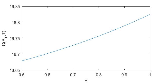
Figure 1. The variation of the geometric Asian option with respect to the Husrt parameter H𝐻H.
Refer to caption
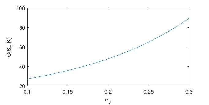
Figure 2. The variation of the geometric Asian option with respect to the σJsubscript𝜎𝐽\sigma_{J}.
Refer to caption
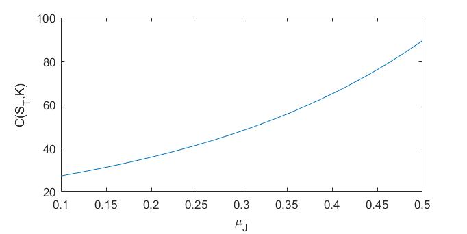
Figure 3. The variation of the geometric Asian option with respect to the μJsubscript𝜇𝐽\mu_{J}.

In Figs 1-3 we show the price of the geometric Asian option computed using formula (2.10) as a function of the Hurst and the jump parameters.
Refer to caption
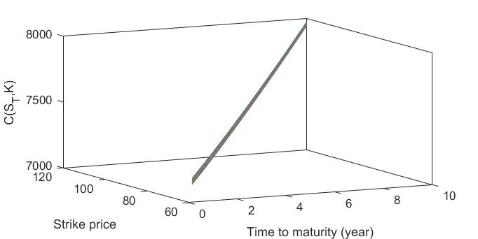
Figure 4. The variation of the geometric Asian option with respect to the strike price K𝐾K and time to maturity (year) T𝑇T.

In Fig 4 we show the price of the geometric Asian option computed using formula (2.10) as a function of the strike price and of the maturity.

3. Arithmetic Asian option

Lemma 3.1.

([24])

An approximate value of the arithmetic Asian option is given by

(3.1) C~(ST,K)~𝐶subscript𝑆𝑇𝐾\displaystyle\tilde{C}(S_{T},K) =\displaystyle= erTE[(G(T)K)+],superscript𝑒𝑟𝑇𝐸delimited-[]superscript𝐺𝑇superscript𝐾\displaystyle e^{-rT}E\left[(G(T)-K^{\prime})^{+}\right],

where G(T)𝐺𝑇G(T) ia the geometric Asian option and Ksuperscript𝐾K^{\prime} is the adjusted strike price as follows

(3.2) K=K(E[A]E[G]).superscript𝐾𝐾𝐸delimited-[]𝐴𝐸delimited-[]𝐺\displaystyle K^{\prime}=K-\left(E[A]-E[G]\right).

Now, based on the actuarial approach an approximate of the arithmetic Asian options are proposed [23, 11].

Theorem 3.1.

An approximate value of the arithmetic Asian option is given by

(3.3) C~(ST,K)~𝐶subscript𝑆𝑇𝐾\displaystyle\tilde{C}(S_{T},K) =\displaystyle=
=\displaystyle= n=0(λT)neλTn![e(rq)Tλ(ρ1)T+μ^+12σ^2Φ(d1)KerTΦ(d2)],superscriptsubscript𝑛0superscript𝜆𝑇𝑛superscript𝑒𝜆𝑇𝑛delimited-[]superscript𝑒𝑟𝑞𝑇𝜆𝜌1𝑇^𝜇12superscript^𝜎2Φsubscript𝑑1superscript𝐾superscript𝑒𝑟𝑇Φsubscript𝑑2\displaystyle\sum_{n=0}^{\infty}\frac{(\lambda T)^{n}e^{-\lambda T}}{n!}\left[e^{-(r-q)T-\lambda(\rho-1)T+\hat{\mu}+\frac{1}{2}\hat{\sigma}^{2}}\Phi(d_{1})-K^{\prime}e^{-rT}\Phi(d_{2})\right],

for the call options, and

(3.4) P~(ST,K)~𝑃subscript𝑆𝑇𝐾\displaystyle\tilde{P}(S_{T},K) =\displaystyle=
=\displaystyle= n=0(λT)neλTn![KerTΦ(d2)e(rq)Tλ(ρ1)T+μ^+12σ^2Φ(d1)],superscriptsubscript𝑛0superscript𝜆𝑇𝑛superscript𝑒𝜆𝑇𝑛delimited-[]superscript𝐾superscript𝑒𝑟𝑇Φsubscript𝑑2superscripte𝑟𝑞𝑇𝜆𝜌1𝑇^𝜇12superscript^𝜎2Φsubscript𝑑1\displaystyle\sum_{n=0}^{\infty}\frac{(\lambda T)^{n}e^{-\lambda T}}{n!}\left[K^{\prime}e^{-rT}\Phi(-d_{2})-\mathrm{e}^{-(r-q)T-\lambda(\rho-1)T+\hat{\mu}+\frac{1}{2}\hat{\sigma}^{2}}\Phi(-d_{1})\right],

for the put options, where

d2=μ^lnUσ^,d1=d2+σ^,formulae-sequencesubscript𝑑2^𝜇𝑈^𝜎subscript𝑑1subscript𝑑2^𝜎\displaystyle d_{2}=\frac{\hat{\mu}-\ln U}{\hat{\sigma}},\,d_{1}=d_{2}+\hat{\sigma},
ρ=E(eJ)=eμJ+12σJ2,U=KeqT(1ρ)λT,formulae-sequence𝜌𝐸superscript𝑒𝐽superscript𝑒subscript𝜇𝐽12superscriptsubscript𝜎𝐽2𝑈superscript𝐾superscript𝑒𝑞𝑇1𝜌𝜆𝑇\displaystyle\rho=E(e^{J})=e^{\mu_{J}+\frac{1}{2}\sigma_{J}^{2}},\,U=K^{\prime}e^{-qT-(1-\rho)\lambda T},
μ^=lnS0+12(rn12σn2)T,μ¯=S0rnT(ernT1)formulae-sequence^𝜇subscript𝑆012subscript𝑟𝑛12superscriptsubscript𝜎𝑛2𝑇¯𝜇subscript𝑆0subscript𝑟𝑛𝑇superscript𝑒subscript𝑟𝑛𝑇1\displaystyle\hat{\mu}=\ln S_{0}+\frac{1}{2}(r_{n}-\frac{1}{2}\sigma_{n}^{2})T,\,\bar{\mu}=\frac{S_{0}}{r_{n}T}\left(e^{r_{n}T}-1\right)
σ^2=σn2T3,σn2=σ2+1T(ε2T2H+nσJ2)formulae-sequencesuperscript^𝜎2superscriptsubscript𝜎𝑛2𝑇3superscriptsubscript𝜎𝑛2superscript𝜎21𝑇superscript𝜀2superscript𝑇2𝐻𝑛superscriptsubscript𝜎𝐽2\displaystyle\hat{\sigma}^{2}=\sigma_{n}^{2}\frac{T}{3},\,\sigma_{n}^{2}=\sigma^{2}+\frac{1}{T}(\varepsilon^{2}T^{2H}+n\sigma_{J}^{2})
(3.5) K=K+E[G]μ¯,rn=rq+nT(μJ+12σJ2),E[G]=eμ^+12σ^2.formulae-sequencesuperscript𝐾𝐾𝐸delimited-[]𝐺¯𝜇formulae-sequencesubscript𝑟𝑛𝑟𝑞𝑛𝑇subscript𝜇𝐽12superscriptsubscript𝜎𝐽2𝐸delimited-[]𝐺superscript𝑒^𝜇12superscript^𝜎2\displaystyle K^{\prime}=K+E[G]-\bar{\mu},\,r_{n}=r-q+\frac{n}{T}(\mu_{J}+\frac{1}{2}\sigma_{J}^{2}),\leavevmode\nobreak\ E[G]=e^{\hat{\mu}+\frac{1}{2}\hat{\sigma}^{2}}.

and Φ(.)\Phi(.) is cumulative normal density function.

Proof.

Suppose

(3.6) A(T)=1T0TSt𝑑t𝐴𝑇1𝑇superscriptsubscript0𝑇subscript𝑆𝑡differential-d𝑡\displaystyle A(T)=\frac{1}{T}\int_{0}^{T}S_{t}dt

be an arithmetic average with mean μ¯=E[A(T)]¯𝜇𝐸delimited-[]𝐴𝑇\bar{\mu}=E\left[A(T)\right], then from Lemma 2.1 we can get

(3.7) μ¯¯𝜇\displaystyle\bar{\mu} =\displaystyle= E[A(T)]=1T0TE[ST]𝑑t𝐸delimited-[]𝐴𝑇1𝑇superscriptsubscript0𝑇𝐸delimited-[]subscript𝑆𝑇differential-d𝑡\displaystyle E\left[A(T)\right]=\frac{1}{T}\int_{0}^{T}E\left[S_{T}\right]dt
=\displaystyle= S0T0Ternt𝑑tsubscript𝑆0𝑇superscriptsubscript0𝑇superscript𝑒subscript𝑟𝑛𝑡differential-d𝑡\displaystyle\frac{S_{0}}{T}\int_{0}^{T}e^{{r_{n}t}}dt
=\displaystyle= S0rnT(ernT1).subscript𝑆0subscript𝑟𝑛𝑇superscript𝑒subscript𝑟𝑛𝑇1\displaystyle\frac{S_{0}}{r_{n}T}\left(e^{r_{n}T}-1\right).

From Theorem 3.1, to provide an approximation of the arithmetic Asian options, we need to calculate the new exercise price Ksuperscript𝐾K^{\prime},

(3.8) Ksuperscript𝐾\displaystyle K^{\prime} =\displaystyle= K(E[A]E[G])𝐾𝐸delimited-[]𝐴𝐸delimited-[]𝐺\displaystyle K-\left(E[A]-E[G]\right)
=\displaystyle= K+E[G]μ¯,𝐾𝐸delimited-[]𝐺¯𝜇\displaystyle K+E[G]-\bar{\mu},

where E[G]=eμ^+12σ^2𝐸delimited-[]𝐺superscript𝑒^𝜇12superscript^𝜎2E[G]=e^{\hat{\mu}+\frac{1}{2}\hat{\sigma}^{2}} is calculated in Theorem 2.1. Now, by replacing K𝐾K with Ksuperscript𝐾K^{\prime} in the proof of Theorem 2.1, the proof is completed. ∎

Suppose, G𝐺G and A𝐴A be the geometric and arithmetic average, respectively. Since the geometric average is less than the arithmetic average, G<A𝐺𝐴G<A, the geometric option price is a lower bound for the arithmetic option price

(3.9) CG=erTE[(GK)+]erTE[(AK)+]=CA.subscript𝐶𝐺superscript𝑒𝑟𝑇𝐸delimited-[]superscript𝐺𝐾superscript𝑒𝑟𝑇𝐸delimited-[]superscript𝐴𝐾subscript𝐶𝐴\displaystyle C_{G}=e^{-rT}E\left[(G-K)^{+}\right]\leq e^{-rT}E\left[(A-K)^{+}\right]=C_{A}.

The inequality

(3.10) max(AK,0)𝐴𝐾0\displaystyle\max(A-K,0) =\displaystyle= max(GK,GA)+AG𝐺𝐾𝐺𝐴𝐴𝐺\displaystyle\max(G-K,G-A)+A-G
\displaystyle\leq max(GK,0)+AG,𝐺𝐾0𝐴𝐺\displaystyle\max(G-K,0)+A-G,

leads to the upper bound

erTE[max(GK,0)+AG]superscript𝑒𝑟𝑇𝐸delimited-[]𝐺𝐾0𝐴𝐺\displaystyle e^{-rT}E\left[\max(G-K,0)+A-G\right]
=erT{E[max(GK)+]+E[A]E[G]}\displaystyle=e^{-rT}\left\{E\left[\max(G-K)^{+}\right]+E[A]-E[G]\right\}
(3.11) =CG+erT(E[A]E[G]).absentsubscript𝐶𝐺superscript𝑒𝑟𝑇𝐸delimited-[]𝐴𝐸delimited-[]𝐺\displaystyle=C_{G}+e^{-rT}\left(E[A]-E[G]\right).

Therefore, we have the following bounds on the arithmetic option price

(3.12) CGCACG+erT(E[A]E[G]).subscript𝐶𝐺subscript𝐶𝐴subscript𝐶𝐺superscript𝑒𝑟𝑇𝐸delimited-[]𝐴𝐸delimited-[]𝐺\displaystyle C_{G}\leq C_{A}\leq C_{G}+e^{-rT}\left(E[A]-E[G]\right).

To compute the upper bound we need to compute the mean of arithmetic average, which is obtained in Theorem 3.1.

Theorem 3.2.

The pricing error of arithmetic approximate vale C~~𝐶\tilde{C} is given by

(3.13) |C~CA|~𝐶subscript𝐶𝐴\displaystyle|\tilde{C}-C_{A}| =\displaystyle= erT(E[A]E[G]).superscript𝑒𝑟𝑇𝐸delimited-[]𝐴𝐸delimited-[]𝐺\displaystyle e^{-rT}\left(E[A]-E[G]\right).
Proof.

Sine

(3.14) max(GK,0)𝐺𝐾0\displaystyle\max(G-K,0) \displaystyle\leq max(GK+E[A]E[G],0)𝐺𝐾𝐸delimited-[]𝐴𝐸delimited-[]𝐺0\displaystyle\max\left(G-K+E[A]-E[G],0\right)
=\displaystyle= max(GK+E[G]E[A])+E[A]E[G]𝐺𝐾𝐸delimited-[]𝐺𝐸delimited-[]𝐴𝐸delimited-[]𝐴𝐸delimited-[]𝐺\displaystyle\max\left(G-K+E[G]-E[A]\right)+E[A]-E[G]
\displaystyle\leq max(GK,0)+E[A]E[G],𝐺𝐾0𝐸delimited-[]𝐴𝐸delimited-[]𝐺\displaystyle\max\left(G-K,0\right)+E[A]-E[G],

it follows that

(3.15) CGsubscript𝐶𝐺\displaystyle C_{G} =\displaystyle= erTE[(GK)+]superscript𝑒𝑟𝑇𝐸delimited-[]superscript𝐺𝐾\displaystyle e^{-rT}E\left[(G-K)^{+}\right]
\displaystyle\leq erTE[(GK+E[A]E[G])+]superscript𝑒𝑟𝑇𝐸delimited-[]superscript𝐺𝐾𝐸delimited-[]𝐴𝐸delimited-[]𝐺\displaystyle e^{-rT}E\left[(G-K+E[A]-E[G])^{+}\right]
=\displaystyle= C~~𝐶\displaystyle\tilde{C}
\displaystyle\leq erTE[(GK)++E[A]E[G]]superscript𝑒𝑟𝑇𝐸delimited-[]superscript𝐺𝐾𝐸delimited-[]𝐴𝐸delimited-[]𝐺\displaystyle e^{-rT}E\left[(G-K)^{+}+E[A]-E[G]\right]
=\displaystyle= CG+erT(E[A]E[G]).subscript𝐶𝐺superscript𝑒𝑟𝑇𝐸delimited-[]𝐴𝐸delimited-[]𝐺\displaystyle C_{G}+e^{-rT}\left(E[A]-E[G]\right).

The analogous bounds exert for the exact value CAsubscript𝐶𝐴C_{A}, then the absolute difference between C~~𝐶\tilde{C} and CAsubscript𝐶𝐴C_{A} is less than the difference between the upper and lower bounds

(3.16) |C~CA|~𝐶subscript𝐶𝐴\displaystyle|\tilde{C}-C_{A}| \displaystyle\leq CG+erT(E[A]E[G])CGsubscript𝐶𝐺superscript𝑒𝑟𝑇𝐸delimited-[]𝐴𝐸delimited-[]𝐺subscript𝐶𝐺\displaystyle C_{G}+e^{-rT}\left(E[A]-E[G]\right)-C_{G}
=\displaystyle= erT(E[A]E[G]).superscript𝑒𝑟𝑇𝐸delimited-[]𝐴𝐸delimited-[]𝐺\displaystyle e^{-rT}\left(E[A]-E[G]\right).

4. Asian power options

This section is deals with evaluate Asian power options by using actuarial approach in a mixed fractional Brownian motion with jumps environment. From [some references], we know that the payoff function of Asian options is given by (Gm(T)K)+superscriptsuperscript𝐺𝑚𝑇𝐾(G^{m}(T)-K)^{+} and (Am(T)K)+superscriptsuperscript𝐴𝑚𝑇𝐾(A^{m}(T)-K)^{+} for the geometric and arithmetic call options with some integer m1𝑚1m\geq 1, respectively.

Theorem 4.1.

Let the stock price S(T)𝑆𝑇S(T) satisfy Equation (2.2). Then, the value of geometric Asian power options with exercise price K𝐾K is given by

(4.1) C(ST,K)𝐶subscript𝑆𝑇𝐾\displaystyle C(S_{T},K) =\displaystyle=
=\displaystyle= n=0(λT)neλTn![e(rq)Tλ(ρ1)T+mμ^+12m2σ^2Φ(d1)KerTΦ(d2)],superscriptsubscript𝑛0superscript𝜆𝑇𝑛superscript𝑒𝜆𝑇𝑛delimited-[]superscript𝑒𝑟𝑞𝑇𝜆𝜌1𝑇𝑚^𝜇12superscript𝑚2superscript^𝜎2Φsubscript𝑑1𝐾superscript𝑒𝑟𝑇Φsubscript𝑑2\displaystyle\sum_{n=0}^{\infty}\frac{(\lambda T)^{n}e^{-\lambda T}}{n!}\left[e^{-(r-q)T-\lambda(\rho-1)T+m\hat{\mu}+\frac{1}{2}m^{2}\hat{\sigma}^{2}}\Phi(d_{1})-Ke^{-rT}\Phi(d_{2})\right],

for the call options, and

(4.2) P(ST,K)𝑃subscript𝑆𝑇𝐾\displaystyle P(S_{T},K) =\displaystyle=
=\displaystyle= n=0(λT)neλTn![KerTΦ(d2)e(rq)Tλ(ρ1)T+mμ^+12m2σ^2Φ(d1)],superscriptsubscript𝑛0superscript𝜆𝑇𝑛superscript𝑒𝜆𝑇𝑛delimited-[]𝐾superscript𝑒𝑟𝑇Φsubscript𝑑2superscripte𝑟𝑞𝑇𝜆𝜌1𝑇𝑚^𝜇12superscript𝑚2superscript^𝜎2Φsubscript𝑑1\displaystyle\sum_{n=0}^{\infty}\frac{(\lambda T)^{n}e^{-\lambda T}}{n!}\left[Ke^{-rT}\Phi(-d_{2})-\mathrm{e}^{-(r-q)T-\lambda(\rho-1)T+m\hat{\mu}+\frac{1}{2}m^{2}\hat{\sigma}^{2}}\Phi(-d_{1})\right],

for the put options, where d2=μ^lnU1nσ^subscript𝑑2^𝜇superscript𝑈1𝑛^𝜎d_{2}=\frac{\hat{\mu}-\ln U^{\frac{1}{n}}}{\hat{\sigma}} and other parameters are defined in Theorem 2.1.

Proof.

For the geometric Asian power options, the payoff function is (Gm(T)K)+=(emL(T)K)+superscriptsuperscript𝐺𝑚𝑇𝐾superscriptsuperscript𝑒𝑚𝐿𝑇𝐾(G^{m}(T)-K)^{+}=(e^{mL(T)}-K)^{+}. Using the strategy given in proof of Theorem 2.1, then we have

(4.3) C(ST,K)𝐶subscript𝑆𝑇𝐾\displaystyle C(S_{T},K) =\displaystyle= E[(exp(0Tθ(t)𝑑t)Gm(T)KerT)IB]𝐸delimited-[]superscriptsubscript0𝑇𝜃𝑡differential-d𝑡superscript𝐺𝑚𝑇𝐾superscript𝑒𝑟𝑇subscript𝐼𝐵\displaystyle E\left[\left(\exp\left(-\int_{0}^{T}\theta(t)dt\right)G^{m}(T)-Ke^{-rT}\right)I_{B}\right]
=\displaystyle= E[(e(rq)Tλ(ρ1)TGm(T)KerT)IB]𝐸delimited-[]superscript𝑒𝑟𝑞𝑇𝜆𝜌1𝑇superscript𝐺𝑚𝑇𝐾superscript𝑒𝑟𝑇subscript𝐼𝐵\displaystyle E\left[\left(e^{-(r-q)T-\lambda(\rho-1)T}G^{m}(T)-Ke^{-rT}\right)I_{B}\right]
=\displaystyle= e(rq)Tλ(ρ1)TE[Gm(T)IB]KerTE[IB]superscript𝑒𝑟𝑞𝑇𝜆𝜌1𝑇𝐸delimited-[]superscript𝐺𝑚𝑇subscript𝐼𝐵𝐾superscript𝑒𝑟𝑇𝐸delimited-[]subscript𝐼𝐵\displaystyle e^{-(r-q)T-\lambda(\rho-1)T}E\left[G^{m}(T)I_{B}\right]-Ke^{-rT}E\left[I_{B}\right]
=\displaystyle= e(rq)Tλ(ρ1)TI1KerTI2,superscript𝑒𝑟𝑞𝑇𝜆𝜌1𝑇subscript𝐼1𝐾superscript𝑒𝑟𝑇subscript𝐼2\displaystyle e^{-(r-q)T-\lambda(\rho-1)T}I_{1}-Ke^{-rT}I_{2},

where I1=E[A(T)IB]subscript𝐼1𝐸delimited-[]𝐴𝑇subscript𝐼𝐵I_{1}=E\left[A(T)I_{B}\right] and I2=E[IB]subscript𝐼2𝐸delimited-[]subscript𝐼𝐵I_{2}=E\left[I_{B}\right]. Let

(4.4) B𝐵\displaystyle B =\displaystyle= {x:emx>U=KeqT(1ρ)λT}conditional-set𝑥superscript𝑒𝑚𝑥𝑈𝐾superscript𝑒𝑞𝑇1𝜌𝜆𝑇\displaystyle\left\{x:e^{mx}>U=Ke^{-qT-(1-\rho)\lambda T}\right\}
=\displaystyle= {x:Gm(T)>U}conditional-set𝑥superscript𝐺𝑚𝑇𝑈\displaystyle\left\{x:G^{m}(T)>U\right\}
=\displaystyle= {y:em(μ^+σ^y)>U}={y:m(μ^+σ^y)>lnU}conditional-set𝑦superscript𝑒𝑚^𝜇^𝜎𝑦𝑈conditional-set𝑦𝑚^𝜇^𝜎𝑦𝑈\displaystyle\left\{y:e^{m(\hat{\mu}+\hat{\sigma}y)}>U\right\}=\left\{y:m(\hat{\mu}+\hat{\sigma}y)>\ln U\right\}
=\displaystyle= {y:y>d2=lnU1mμ^σ^}.conditional-set𝑦𝑦subscript𝑑2superscript𝑈1𝑚^𝜇^𝜎\displaystyle\left\{y:y>-d_{2}=\frac{\ln U^{\frac{1}{m}}-\hat{\mu}}{\hat{\sigma}}\right\}.

Observe that

(4.5) I2subscript𝐼2\displaystyle I_{2} =\displaystyle= E[IB]=n=0E[IGm(T)>d2]P[NT=n]𝐸delimited-[]subscript𝐼𝐵superscriptsubscript𝑛0𝐸delimited-[]subscript𝐼superscript𝐺𝑚𝑇subscript𝑑2𝑃delimited-[]subscript𝑁𝑇𝑛\displaystyle E\left[I_{B}\right]=\sum_{n=0}^{\infty}E\left[I_{G^{m}(T)>-d_{2}}\right]P\left[N_{T}=n\right]
=\displaystyle= n=0(λT)neλTn!E[IGm(T)>d2]superscriptsubscript𝑛0superscript𝜆𝑇𝑛superscript𝑒𝜆𝑇𝑛𝐸delimited-[]subscript𝐼superscript𝐺𝑚𝑇subscript𝑑2\displaystyle\sum_{n=0}^{\infty}\frac{(\lambda T)^{n}e^{-\lambda T}}{n!}E\left[I_{G^{m}(T)>-d_{2}}\right]
=\displaystyle= n=0(λT)neλTn!d2ϕ(y)𝑑ysuperscriptsubscript𝑛0superscript𝜆𝑇𝑛superscript𝑒𝜆𝑇𝑛superscriptsubscriptsubscript𝑑2italic-ϕ𝑦differential-d𝑦\displaystyle\sum_{n=0}^{\infty}\frac{(\lambda T)^{n}e^{-\lambda T}}{n!}\int_{-d_{2}}^{\infty}\phi(y)dy
=\displaystyle= n=0(λT)neλTn!Φ(d2),superscriptsubscript𝑛0superscript𝜆𝑇𝑛superscript𝑒𝜆𝑇𝑛Φsubscript𝑑2\displaystyle\sum_{n=0}^{\infty}\frac{(\lambda T)^{n}e^{-\lambda T}}{n!}\Phi(d_{2}),

and

(4.6) I1subscript𝐼1\displaystyle I_{1} =\displaystyle= E[Gm(T)IB]=n=0E[Gm(T)IGm(T)>d2]P[NT=n]𝐸delimited-[]superscript𝐺𝑚𝑇subscript𝐼𝐵superscriptsubscript𝑛0𝐸delimited-[]superscript𝐺𝑚𝑇subscript𝐼superscript𝐺𝑚𝑇subscript𝑑2𝑃delimited-[]subscript𝑁𝑇𝑛\displaystyle E\left[G^{m}(T)I_{B}\right]=\sum_{n=0}^{\infty}E\left[G^{m}(T)I_{G^{m}(T)>-d_{2}}\right]P\left[N_{T}=n\right]
=\displaystyle= n=0(λT)neλTn!E[emL(T)IGm(T)>d2]superscriptsubscript𝑛0superscript𝜆𝑇𝑛superscript𝑒𝜆𝑇𝑛𝐸delimited-[]superscript𝑒𝑚𝐿𝑇subscript𝐼superscript𝐺𝑚𝑇subscript𝑑2\displaystyle\sum_{n=0}^{\infty}\frac{(\lambda T)^{n}e^{-\lambda T}}{n!}E\left[e^{mL(T)}I_{G^{m}(T)>-d_{2}}\right]
=\displaystyle= n=0(λT)neλTn!Bemx12πσ^e(xμ^)22σ^2𝑑xsuperscriptsubscript𝑛0superscript𝜆𝑇𝑛superscript𝑒𝜆𝑇𝑛subscript𝐵superscript𝑒𝑚𝑥12𝜋^𝜎superscript𝑒superscript𝑥^𝜇22superscript^𝜎2differential-d𝑥\displaystyle\sum_{n=0}^{\infty}\frac{(\lambda T)^{n}e^{-\lambda T}}{n!}\int_{B}e^{mx}\frac{1}{\sqrt{2\pi}\hat{\sigma}}e^{-\frac{(x-\hat{\mu})^{2}}{2\hat{\sigma}^{2}}}dx
=\displaystyle= n=0(λT)neλTn!Bem(μ^+σ^y)12πσ^e(xμ^)22σ^2𝑑ysuperscriptsubscript𝑛0superscript𝜆𝑇𝑛superscript𝑒𝜆𝑇𝑛subscript𝐵superscript𝑒𝑚^𝜇^𝜎𝑦12𝜋^𝜎superscript𝑒superscript𝑥^𝜇22superscript^𝜎2differential-d𝑦\displaystyle\sum_{n=0}^{\infty}\frac{(\lambda T)^{n}e^{-\lambda T}}{n!}\int_{B}e^{m(\hat{\mu}+\hat{\sigma}y)}\frac{1}{\sqrt{2\pi}\hat{\sigma}}e^{-\frac{(x-\hat{\mu})^{2}}{2\hat{\sigma}^{2}}}dy
=\displaystyle= n=0(λT)neλTn!emμ^+12m2σ^2d212πe12(ymσ^)2𝑑ysuperscriptsubscript𝑛0superscript𝜆𝑇𝑛superscript𝑒𝜆𝑇𝑛superscript𝑒𝑚^𝜇12superscript𝑚2superscript^𝜎2superscriptsubscriptsubscript𝑑212𝜋superscript𝑒12superscript𝑦𝑚^𝜎2differential-d𝑦\displaystyle\sum_{n=0}^{\infty}\frac{(\lambda T)^{n}e^{-\lambda T}}{n!}e^{m\hat{\mu}+\frac{1}{2}m^{2}\hat{\sigma}^{2}}\int_{-d_{2}}^{\infty}\frac{1}{\sqrt{2\pi}}e^{-\frac{1}{2}(y-m\hat{\sigma})^{2}}dy
=\displaystyle= n=0(λT)neλTn!emμ^+12m2σ^2d2σ^ϕ(y)𝑑ysuperscriptsubscript𝑛0superscript𝜆𝑇𝑛superscript𝑒𝜆𝑇𝑛superscript𝑒𝑚^𝜇12superscript𝑚2superscript^𝜎2superscriptsubscriptsubscript𝑑2^𝜎italic-ϕ𝑦differential-d𝑦\displaystyle\sum_{n=0}^{\infty}\frac{(\lambda T)^{n}e^{-\lambda T}}{n!}e^{m\hat{\mu}+\frac{1}{2}m^{2}\hat{\sigma}^{2}}\int_{-d_{2}-\hat{\sigma}}^{\infty}\phi(y)dy
=\displaystyle= n=0(λT)neλTn!emμ^+12m2σ^2Φ(d1=d2+σ^).superscriptsubscript𝑛0superscript𝜆𝑇𝑛superscript𝑒𝜆𝑇𝑛superscript𝑒𝑚^𝜇12superscript𝑚2superscript^𝜎2Φsubscript𝑑1subscript𝑑2^𝜎\displaystyle\sum_{n=0}^{\infty}\frac{(\lambda T)^{n}e^{-\lambda T}}{n!}e^{m\hat{\mu}+\frac{1}{2}m^{2}\hat{\sigma}^{2}}\Phi(d_{1}=d_{2}+\hat{\sigma}).

From Eqs. (4.3), (4.5) and (4.6), we get desired result.

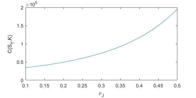
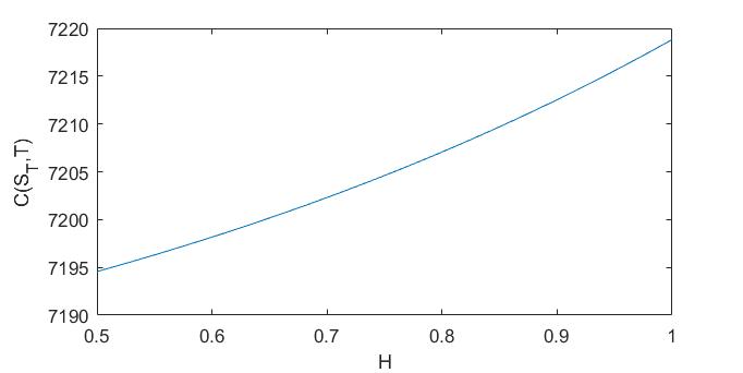
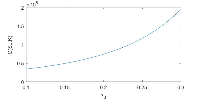
In Figs 5-7 we show the price of the power Asian option computed using formula 4.1 as a function of the Hurst and the jump. parameters.
Refer to caption
Figure 5. The variation of the power Asian option with respect to the Husrt parameter H𝐻H.
Refer to caption
Figure 6. The variation of the power Asian option with respect to the σJsubscript𝜎𝐽\sigma_{J}

.

Refer to caption
Figure 7. The variation of the power Asian option with respect to the μJsubscript𝜇𝐽\mu_{J}

.

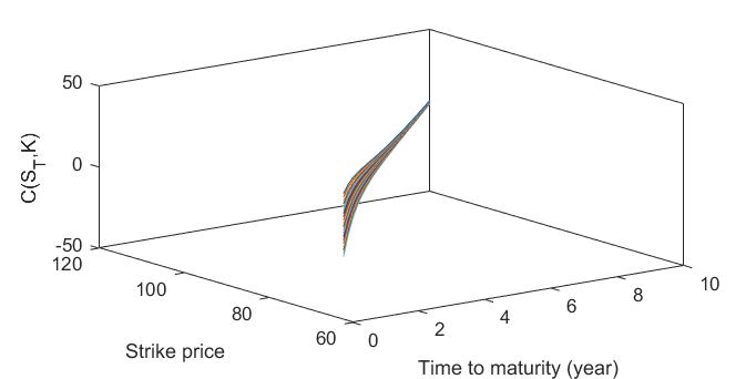
Refer to caption
Figure 8. The variation of the power Asian option with respect to the both strike price K𝐾K and time to maturity (year) T𝑇T.

In Fig 8 we show the price of the power Asian option computed using formula 4.1 as a function of the strike price and of the maturity.

The payoff function of the power Asian power call option is (Am(T)K)superscript𝐴𝑚𝑇𝐾(A^{m}(T)-K), then its approximate value is given by the following theorem.

Theorem 4.2.

An approximate value of the arithmetic Asian power option is given by

(4.7) C~(ST,K)~𝐶subscript𝑆𝑇𝐾\displaystyle\tilde{C}(S_{T},K) =\displaystyle=
=\displaystyle= n=0(λT)neλTn![e(rq)Tλ(ρ1)T+μ^+12σ^2Φ(d1)KerTΦ(d2)],superscriptsubscript𝑛0superscript𝜆𝑇𝑛superscript𝑒𝜆𝑇𝑛delimited-[]superscript𝑒𝑟𝑞𝑇𝜆𝜌1𝑇^𝜇12superscript^𝜎2Φsubscript𝑑1superscript𝐾superscript𝑒𝑟𝑇Φsubscript𝑑2\displaystyle\sum_{n=0}^{\infty}\frac{(\lambda T)^{n}e^{-\lambda T}}{n!}\left[e^{-(r-q)T-\lambda(\rho-1)T+\hat{\mu}+\frac{1}{2}\hat{\sigma}^{2}}\Phi(d_{1})-K^{\prime}e^{-rT}\Phi(d_{2})\right],

for the call options, and

(4.8) P~(ST,K)~𝑃subscript𝑆𝑇𝐾\displaystyle\tilde{P}(S_{T},K) =\displaystyle=
=\displaystyle= n=0(λT)neλTn![KerTΦ(d2)e(rq)Tλ(ρ1)T+μ^+12σ^2Φ(d1)],superscriptsubscript𝑛0superscript𝜆𝑇𝑛superscript𝑒𝜆𝑇𝑛delimited-[]superscript𝐾superscript𝑒𝑟𝑇Φsubscript𝑑2superscripte𝑟𝑞𝑇𝜆𝜌1𝑇^𝜇12superscript^𝜎2Φsubscript𝑑1\displaystyle\sum_{n=0}^{\infty}\frac{(\lambda T)^{n}e^{-\lambda T}}{n!}\left[K^{\prime}e^{-rT}\Phi(-d_{2})-\mathrm{e}^{-(r-q)T-\lambda(\rho-1)T+\hat{\mu}+\frac{1}{2}\hat{\sigma}^{2}}\Phi(-d_{1})\right],

for the put options, where d2=μ^lnU1mσ^subscript𝑑2^𝜇superscript𝑈1𝑚^𝜎d_{2}=\frac{\hat{\mu}-\ln U^{\frac{1}{m}}}{\hat{\sigma}} and other parameters are defined in Theorem 3.1.

Proof.

Suppose μ¯=E[Am(T)]¯𝜇𝐸delimited-[]superscript𝐴𝑚𝑇\bar{\mu}=E\left[A^{m}(T)\right], then

(4.9) μ¯¯𝜇\displaystyle\bar{\mu} =\displaystyle= E[Am(T)]=1T0TE[(Stn)m]𝑑t𝐸delimited-[]superscript𝐴𝑚𝑇1𝑇superscriptsubscript0𝑇𝐸delimited-[]superscriptsuperscriptsubscript𝑆𝑡𝑛𝑚differential-d𝑡\displaystyle E\left[A^{m}(T)\right]=\frac{1}{T}\int_{0}^{T}E\left[(S_{t}^{n})^{m}\right]dt
=\displaystyle= S0T0Tem((rn12σn2)t+12mσn2t)=S0mT0Temrnt𝑑tsubscript𝑆0𝑇superscriptsubscript0𝑇superscript𝑒𝑚subscript𝑟𝑛12superscriptsubscript𝜎𝑛2𝑡12𝑚superscriptsubscript𝜎𝑛2𝑡superscriptsubscript𝑆0𝑚𝑇superscriptsubscript0𝑇superscript𝑒𝑚subscript𝑟𝑛𝑡differential-d𝑡\displaystyle\frac{S_{0}}{T}\int_{0}^{T}e^{m((r_{n}-\frac{1}{2}\sigma_{n}^{2})t+\frac{1}{2}m\sigma_{n}^{2}t)}=\frac{S_{0}^{m}}{T}\int_{0}^{T}e^{mr_{n}t}dt
=\displaystyle= S0mmrnT(emrnT1).superscriptsubscript𝑆0𝑚𝑚subscript𝑟𝑛𝑇superscript𝑒𝑚subscript𝑟𝑛𝑇1\displaystyle\frac{S_{0}^{m}}{mr_{n}T}\left(e^{mr_{n}T}-1\right).

From Theorem [24], to provide an approximation of the arithmetic Asian power options, we need to calculate the new exercise price Ksuperscript𝐾K^{\prime},

(4.10) Ksuperscript𝐾\displaystyle K^{\prime} =\displaystyle= K(E[Am]E[Gm])𝐾𝐸delimited-[]superscript𝐴𝑚𝐸delimited-[]superscript𝐺𝑚\displaystyle K-\left(E[A^{m}]-E[G^{m}]\right)
=\displaystyle= K+E[Gm]μ¯,𝐾𝐸delimited-[]superscript𝐺𝑚¯𝜇\displaystyle K+E[G^{m}]-\bar{\mu},

where E[Gm]=emμ^+12m2σ^2𝐸delimited-[]superscript𝐺𝑚superscript𝑒𝑚^𝜇12superscript𝑚2superscript^𝜎2E[G^{m}]=e^{m\hat{\mu}+\frac{1}{2}m^{2}\hat{\sigma}^{2}} is calculated in Theorem 4.1. Now, by replacing K𝐾K with Ksuperscript𝐾K^{\prime} in the proof of Theorem 4.1, the proof is completed. ∎

5. Conclusions

We derived approximate closed-form solutions for pricing arithmetic Asian options on an underlying described by the mixed fractional Brownian motion (mfBm𝑚𝑓𝐵𝑚mfBm). In the last decade, the mfBm𝑚𝑓𝐵𝑚mfBm has gained increasing popularity in finance, since it allows one to incorporate long-range dependence and self-similarity and, for certain values of the Hurst parameter, it is arbitrage-free. In the present paper, suitable approximate closed-form solutions are obtained for both arithmetic Asian options and arithmetic Asian power options, by applying a convenient approximation of their strike prices. Both the standard mfBm𝑚𝑓𝐵𝑚mfBm and the mfBm𝑚𝑓𝐵𝑚mfBm with Poisson log-normally distributed jumps are considered.

References

  • [1] D. Ahmadian and L. V. Ballestra. Pricing geometric Asian rainbow options under the mixed fractional Brownian motion. Physica A: Statistical Mechanics and its Applications, 555:124458, 2020.
  • [2] L. V. Ballestra, G. Pacelli, and D. Radi. A very efficient approach for pricing barrier options on an underlying described by the mixed fractional Brownian motion. Chaos, Solitons & Fractals, 87:240–248, 2016.
  • [3] C. Bender and R. J. Elliott. Arbitrage in a discrete version of the Wick-fractional Black-Scholes market. Mathematics of Operations Research, 29:935–945, 2004.
  • [4] Mogens Bladt and Tina Hviid Rydberg. An actuarial approach to option pricing under the physical measure and without market assumptions. Insurance: Mathematics and Economics, 22(1):65–73, 1998.
  • [5] J. H Chen, F. Y. Ren, and W. Y. Qiu. Option pricing of a mixed fractional-fractional version of the Black-Scholes model. Chaos, Solitons & Fractals, 21:1163–1174, 2004.
  • [6] P. Cheridito. Mixed fractional Brownian motion. Bernoulli, 7:913–934, 2001.
  • [7] P. Cheridito. Arbitrage in fractional Brownian motion models. Finance and Stochastics, 7:533–553, 2003.
  • [8] Patrick Cheridito. Arbitrage in fractional Brownian motion models. Finance and Stochastics, 7(4):533–553, 2003.
  • [9] Z. Ding, C. W. J. Granger, and R. F. Engle. A long memory property of stock market returns and a new model. Journal of Empirical Finance, 1:83–106, 1993.
  • [10] X. He and W. Chen. The pricing of credit default swaps under a generalized mixed fractional Brownian motion. Physica A: Statistical Mechanics and its Applications, 404:26–33, 2014.
  • [11] Angelien GZ Kemna and Antonius CF Vorst. A pricing method for options based on average asset values. Journal of Banking & Finance, 14(1):113–129, 1990.
  • [12] A. W. Lo. Long-term memory in stock market prices. Econometrica, 59:1279–1313, 1991.
  • [13] Y. S. Mishura. Stochastic Calcular for Fractional Brownian Motion and Related Process. Springer–Verlag, Berlin, 2008.
  • [14] Y. S. Mishura and E. Valkeila. The absence of arbitrage in a mixed Brownian fractional Brownian model. In Proceedings of the Steklov Institute of Mathematics, number 237, pages 224–233. Trudy Matematicheskogo Instituta Imeni V.A. Steklova, 2002.
  • [15] B. Peng and F. Peng. Pricing Asian power options under jump-fraction process. Journal of Economics Finance and Administrative Science, 17:2–9, 2012.
  • [16] B. L. S. Prakasa Rao. Pricing geometric Asian power options under mixed fractional Brownian motion environment. Physica A: Statistical Mechanics and its Applications, 446:92–99, 2012.
  • [17] S. Rostek and R. Schöbel. A note on the use of fractional Brownian motion for financial modeling. Economic Modelling, 30:30–35, 2013.
  • [18] Foad Shokrollahi. The evaluation of geometric Asian power options under time changed mixed fractional Brownian motion. Journal of Computational and Applied Mathematics, 344:716–724, 2018.
  • [19] Foad Shokrollahi and Adem Kılıçman. Pricing currency option in a mixed fractional Brownian motion with jumps environment. Mathematical Problems in Engineering, 2014, 2014.
  • [20] Foad Shokrollahi and Adem Kılıçman. Actuarial approach in a mixed fractional Brownian motion with jumps environment for pricing currency option. Advances in Difference Equations, 2015(1):1–8, 2015.
  • [21] Steven E Shreve. Stochastic calculus for finance II: Continuous-time models, volume 11. Springer Science & Business Media, 2004.
  • [22] L. Sun. Pricing currency options in the mixed fractional Brownian motion. Physica A: Statistical Mechanics and its Applications, 392:3441–3458, 2013.
  • [23] Stuart M Turnbull and Lee Macdonald Wakeman. A quick algorithm for pricing European average options. Journal of Financial and Quantitative Analysis, pages 377–389, 1991.
  • [24] Ton Vorst. Prices and hedge ratios of average exchange rate options. International Review of Financial Analysis, 1(3):179–193, 1992.
  • [25] X.-T. Wang, E.-H. Zhu, M.-M. Tang, and H.-G. Yan. Scaling and long-range dependence in option pricing II: Pricing European option with transaction costs under the mixed Brownian–fractional Brownian model. Physica A: Statistical Mechanics and its Applications, 3:445–451, 2010.
  • [26] W. L. Xiao, W. G. Zhang, X. Zhang, and X. Zhang. Pricing model for equity warrants in a mixed fractional Brownian environment and its algorithm. Physica A: Statistical Mechanics and its Applications, 391:6418–6431, 2012.
  • [27] W. G. Zhang, Z. Li, and Y. J. Liu. Analytical pricing of geometric Asian power options on an underlying driven by a mixed fractional Brownian motion. Physica A: Statistical Mechanics and its Applications, 490:402–418, 2018.
  • [28] M. Zili. On the mixed fractional Brownian motion. Journal of Applied Mathematics and Stochastic Analysis, ID 32435:1–9, 2006.