Analytic and exponentially localized brane-world Reissner-Nordström-AdS solution: a top-down approach

Theodoros Nakas* — and Panagiota Kanti* —

Division of Theoretical Physics, Department of Physics,
University of Ioannina, Ioannina GR-45110, Greece

Abstract

In this work, we construct a five-dimensional spherically-symmetric, charged and asymptotically Anti-de Sitter black hole with its singularity being point-like and strictly localised on our brane. In addition, the induced brane geometry is described by a Reissner-Nordström-(A)dS line-element. We perform a careful classification of the horizons, and demonstrate that all of them are exponentially localised close to the brane thus exhibiting a pancake shape. The bulk gravitational background is everywhere regular, and reduces to an AdS₅ spacetime right outside the black-hole event horizon. This geometry is supported by an anisotropic fluid with only two independent components, the energy density $\rho_{E}$ and tangential pressure $p_{2}$. All energy conditions are respected close to and on our brane, but a local violation takes place within the event horizon regime in the bulk. A tensor-vector-scalar field-theory model is built in an attempt to realise the necessary bulk matter, however, in order to do so, both gauge and scalar degrees of freedom need to turn phantom-like at the bulk boundary. The study of the junction conditions reveals that no additional matter needs to be introduced on the brane for its consistent embedding in the bulk geometry apart from its constant, positive tension. We finally compute the effective gravitational equations on the brane, and demonstrate that the Reissner-Nordström-(A)dS geometry on our brane is caused by the combined effect of the five-dimensional geometry and bulk matter with its charge being in fact a tidal charge.

 

 

1 Prologue

The idea of the existence of extra spacelike dimensions, first suggested by Kaluza [1] and Klein [2], is now more than a hundred years old. During this time interval, it has been employed in order to formulate fundamental theories of particle physics, such as string theory [3, 4], or more phenomenologically-oriented models such as the Large Extra Dimensions [5, 6, 7] or Warped Extra Dimensions [8, 9] scenaria. In the latter two models in particular, our four-dimensional world is a 3-brane [10, 11] embedded in a higher-dimensional spacetime (the bulk). In the Large Extra Dimension scenario [5, 6, 7], the extra spacelike dimensions are compactified to a new length scale—this scale is an independent scale of the theory which however has to be smaller than the $\mu m$ scale in order to avoid observation [12, 13]. In the Warped Extra Dimensions scenario[8, 9], there is only one extra spacelike dimension, which may be either compactified, by introducing a second brane, or assumed to be infinite—in the latter case, the localisation of the graviton close to our brane, ensured by an exponentially decaying warp factor in the metric, leads to an effective compactification of the infinite fifth dimension.

Motivated by the above, a plethora of higher-dimensional studies in both particle physics and gravity were performed over the years. The interest in the construction of black-hole solutions living in an arbitrary number of spacelike dimensions, flat or warped, was intense. In the case of Large Extra Dimensions, the assumed flatness of the higher-dimensional spacetime allowed for previously derived, analytical black-hole solutions [14, 15] to accurately model such gravitational objects also in the new context. In contrast, the warping of the bulk spacetime in the case of the Warped Extra Dimensions scenario posed a significant obstacle in the construction of analytical solutions describing black holes centered on our brane and extending in a regular bulk spacetime. In the first such attempt [16], the effort to construct a five-dimensional brane-world black hole led instead to the emergence of a black-string solution; although the line-element on the brane matched the Schwarzschild solution, its singularity was not point-like and localised on our brane, where the gravitational collapse had taken place, but it was extending along the infinite fifth dimension. This infinitely-long black-string solution was plagued by a curvature singularity at the AdS infinity, thus refuting the gravity localisation, and was also proven to be unstable [17, 18]. Since then, numerous attempts for the construction of a robust brane-world black-hole solution have been made in the literature (for a partial only list, see [19, 20, 21, 22, 23, 24, 25, 26, 27, 28, 29, 30, 31, 32, 33, 34, 35, 36, 37, 38, 39, 40, 41, 42, 43, 44, 45, 46, 47, 48, 49, 50, 51, 52, 53, 54, 55, 56, 57]). Despite these efforts, an exact, analytic solution describing a five-dimensional black hole localised close to our brane and leading also to a Schwarzschild black hole on the brane was never found. The construction, on the other hand, of numerical solutions describing small [58, 59] and large [60, 61, 62] black holes as well as the easiness with which black-string solutions emerge in the context of the same theory (again, for a non-exhaustive list, see [63, 64, 65, 66, 67, 68, 69, 70, 71, 72, 73, 74, 75, 76, 77, 78, 79, 80, 81, 82, 83, 84]) kept vibrant the interest in providing an answer as to what type of geometrical construction could lead to the long-sought brane-world black-hole solution.

In a recent work of ours [85], we have addressed the above question and constructed from first principles, the geometry of an analytic, spherically-symmetric five-dimensional black hole. This was done by combining both bulk and brane perspectives, that is by employing a set of coordinates that ensured the isotropy of the five-dimensional spacetime and combining it with an appropriately selected metric function of the four-dimensional line-element. This geometrical construction resulted into a black-hole solution which had its singularity strictly localised at a single point on the brane. Its horizon was extending into the bulk, as expected, but it had a pancake shape and was localised exponentially close to our brane. The five-dimensional background was everywhere regular and reduced to a pure AdS₅ spacetime right outside the black-hole horizon. This geometric solution was not a vacuum one, and a form of bulk matter had to be introduced in order to support it. However, this bulk matter was characterised by a very simple energy-momentum tensor describing an anisotropic fluid with only two independent components, the energy density and tangential pressure. The geometric background on the brane was of a pure Schwarzschild form, which was shown to satisfy the gravitational field equations of the effective four-dimensional theory.

In the present work, we generalise our previous analysis by retaining the basic method for the construction of the five-dimensional, spherically-symmetric black hole but by considering an alternative form of the metric function. This form is inspired by the one of the four-dimensional Reissner-Nordström-(A)dS solution. In this way, we allow for the presence of a charge term and of a cosmological constant in the effective metric, thus generalising our previous assumption of a neutral, asymptotically-flat brane black hole. However, being also part of a five-dimensional line-element, the richer topological structure following from this new metric function is transferred also in the bulk. Thus, we perform a thorough study of both the horizon structure of the five-dimensional spacetime and of all curvature invariants. We demonstrate that the singularity of the black hole remains point-like and strictly localised on the brane. We also show that every horizon radius characterising the spacetime, depending on the values of its parameters, acquires a pancake shape and gets exponentially localised close to the brane. The five-dimensional spacetime is everywhere regular and reduces again to an AdS₅ spacetime right outside the black hole event horizon. Our analysis remains at all points analytical and manages to accommodate all geometrical features necessary for the localisation of a physical black-hole solution close to our brane. In fact, as we will demonstrate, our constructed line-element has the same general structure as the one used in [61] for the numerical construction of such a solution with the difference that in our case all metric components are analytically known.

We next turn to the question of what is the form of the bulk matter that would support the aforementioned geometry. To this end, we perform a detailed study of the bulk energy-momentum tensor, and show that its minimal structure with only two independent components is preserved also in this case. We then attempt to construct a field-theory model for the realisation of the bulk matter, in the form of a five-dimensional tensor-vector-scalar theory, and discuss the conditions under which such a description could be viable. We then focus on the presence of the brane itself, and we first study the junctions conditions which govern its consistent embedding in the five-dimensional background. We demonstrate that these are satisfied by a brane with no additional matter apart from its positive tension. Finally, we derive the gravitational equations of the effective theory and demonstrate that they are indeed satisfied by the induced solution on the brane, namely the Reissner-Nordström-(A)dS solution.

The structure of this paper is as follows: in Section 2, we present the general method for constructing the five-dimensional geometry and study its geometrical properties. In Section 3, we turn to the gravitational theory, study the profile of the bulk matter and present the field-theory toy model. In Section 4, we investigate the junction conditions and the effective gravitational theory on the brane. We summarise our analysis and discuss our results in Section 5.

2 The Geometrical Setup

We start our analysis with the Randall-Sundrum (RS) metric ansatz [8, 9] which describes a five-dimensional warped spacetime. Its line-element has the form

$$ds^{2}=e^{-2k|y|}\left(-dt^{2}+d\vec{x}^{\,2}\right)+dy^{2}\,.$$ (2.1)

The aforementioned spacetime is comprised by four-dimensional flat slices stacked together along a fifth dimension denoted by the coordinate $y$. The warp factor of each slice is $e^{-2k|y|}$, where $k$ is the curvature of the five-dimensional AdS spacetime. In [8, 9], the AdS bulk spacetime is sourced by a negative five-dimensional cosmological constant. In the context of this work, we will assume that our four-dimensional world is represented by a 3-brane located at $y=0$.

We may also write the above line-element in conformally-flat coordinates: we thus introduce a new bulk coordinate $z$ via the relation $z=sgn(y)\,(e^{k|y|}-1)/k$. In addition, as we will address the presence of localised, spherically-symmetric solutions on our brane, we employ spherical coordinates for the spatial brane directions. Then, the line-element (2.1) takes the form

$$ds^{2}=\frac{1}{(k|z|+1)^{2}}\left(-dt^{2}+dr^{2}+r^{2}\,d\Omega_{2}^{2}+dz^{2}\right)\,,$$ (2.2)

where $d\Omega_{2}^{2}=d\theta^{2}+\sin^{2}\theta\,d\phi^{2}$. As in the original RS models, the bulk-related ${\mathbf{Z}}_{2}$ symmetry under the change $z\rightarrow-z$ has been also preserved here for consistency reasons.

We will now extend the spherical symmetry into the bulk by performing the following change of variables

$$\left\{r=\rho\sin\chi\,,\hskip 5.0ptz=\rho\cos\chi\right\}\,,$$ (2.3)

in terms of which Eq. (2.2) reads

$$ds^{2}=\frac{1}{(1+k\rho|\cos\chi|)^{2}}\left(-dt^{2}+d\rho^{2}+\rho^{2}\,d\Omega_{3}^{2}\right)\,.$$ (2.4)

In the above, $\chi$ is an angular coordinate which takes values in the range $[0,\pi]$, $\rho$ denotes the radial coordinate of the four-dimensional spatial part of the five-dimensional spacetime, while

$$d\Omega_{3}^{2}=d\chi^{2}+\sin^{2}\chi\,d\theta^{2}+\sin^{2}\chi\,\sin^{2}\theta\,d\phi^{2}$$ (2.5)

corresponds to the line-element of a unit 3-sphere. From (2.3) we easily deduce that $\rho$ is always positive definite while the domains $\chi\in\left[0,\pi/2\right)$ and $\chi\in\left(\pi/2,\pi\right]$ correspond to positive and negative values of $z$, respectively. The line-element (2.4) is invariant under the coordinate transformation $\chi\rightarrow\pi-\chi$, which relates the two domains, due to the assumed ${\mathbf{Z}}_{2}$ symmetry. We may therefore focus only on the $\left[0,\pi/2\right]$ domain for which $\cos\chi\geq 0$. The inverse transformation to (2.3) reads

$$\big{\{}\rho=\sqrt{r^{2}+z^{2}}\ ,\quad\tan\chi=r/z\big{\}}\,.$$ (2.6)

From this, we deduce that the radial coordinate $\rho$ ranges over the interval $[0,\infty)$. In fact, it receives contributions both from the (brane) $r$ and (bulk) $z$ coordinates. Therefore, the radial infinity, $\rho\rightarrow\infty$, may describe both the asymptotic AdS boundary ($|z|\rightarrow\infty$) and the radial infinity on the brane ($r\rightarrow\infty$). In the new coordinate system (2.3), the brane, which was located at $y=0$ or $z=0$, now lies at $\cos\chi=0$, i.e. at $\chi=\pi/2$. There, $\rho$ reduces to the brane radial coordinate $r$. The geometrical set-up of the five-dimensional spacetime along with the two systems of coordinates are depicted in Fig. 1.

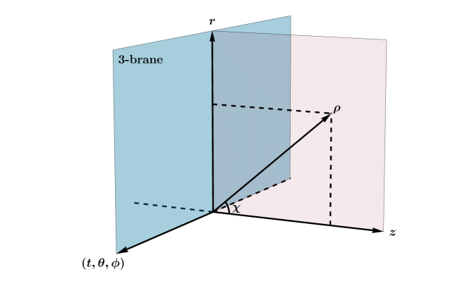
Figure 1: The geometrical set-up of the five-dimensional spacetime and the set of coordinates.

As mentioned previously, we are interested in placing a spherically-symmetric black hole on our brane. To this end, we replace the two-dimensional flat part $(-dt^{2}+d\rho^{2})$ of the line-element in Eq. (2.4) with a curved part, and thus we write

$$ds^{2}=\frac{1}{(1+k\rho\cos\chi)^{2}}\bigg{[}-f(\rho)\,dt^{2}+\frac{d\rho^{2}}{f(\rho)}+\rho^{2}\,d\Omega_{3}^{2}\bigg{]}\,,\hskip 15.00002pt\chi\in[0,\pi/2]\,.$$ (2.7)

Here, $f(\rho)$ is a general spherically-symmetric function. In the context of this work, we are interested in the study of black holes, and we will therefore assume that $f(\rho)$ has a form inspired by the more general spherically-symmetric black-hole solution of General Relativity, namely the Reissner-Nordström-(Anti-)de Sitter solution:

$$f(\rho)=1-\frac{2M}{\rho}+\frac{Q^{2}}{\rho^{2}}-\frac{\Lambda}{3}\,\rho^{2}\,.$$ (2.8)

Note that, on the brane where $\cos\chi=0$ and $\rho=r$, the line-element (2.7) does reduce to a Reissner-Nordström-(Anti-)de Sitter black hole, with the parameter $M$ being related to its mass, $Q$ to its charge and $\Lambda$ to the effective cosmological constant on the brane.

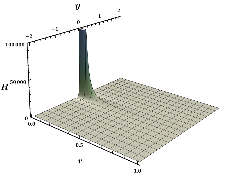
(a)

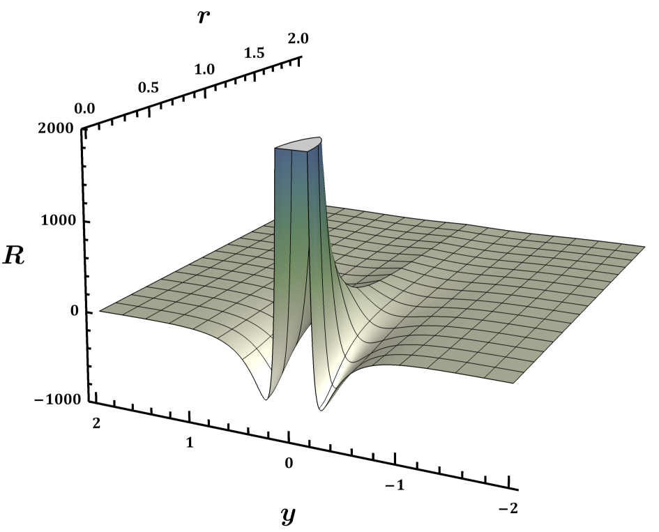
(b)          

Figure 2: (a) The scalar curvature $R$ in terms of the coordinates $(r,y)$ for $k=1$, $M=10$, $Q=1$, and $\Lambda=5\times 10^{-4}$, while (b) shows a magnification of the geometry near the singularity.

However, its interpretation from the bulk point-of-view needs to be carefully examined. Indeed, almost all known analytic black-hole solutions on the brane either lack completely a bulk description, or correspond to bulk solutions with an undesired topology (i.e. that of a black string) or unattractive characteristics (i.e. non-asymptotically AdS solutions). We will therefore investigate now the topological characteristics of our five-dimensional construction. To this end, we compute all scalar gravitational quantities, namely the Ricci scalar $R$, the Ricci tensor combination $\mathcal{R}\equiv R^{MN}R_{MN}$ and the Kretchmann scalar $\mathcal{K}\equiv R^{MNKL}R_{MNKL}$. The expression of the Ricci scalar is the most elegant one and is given below

$$R=-20\left(k^{2}-\frac{\Lambda}{3}\right)+\frac{12k^{2}M\cos^{2}\chi}{\rho}-\frac{12k\cos\chi\left(kQ^{2}\cos\chi+2M\right)}{\rho^{2}}+\frac{4\left(2kQ^{2}\cos\chi+M\right)}{\rho^{3}}\,,$$ (2.9)

while the more extended $\mathcal{R}$ and $\mathcal{K}$ quantities are presented in Appendix A. The above expression contains a constant term which involves the warping parameter $k$ and the effective cosmological parameter $\Lambda$. It also contains additional terms sourced by the mass and charge of the black hole. These terms are singular at the value $\rho=0$ of the bulk radial coordinate. However, this singularity arises only when $r$ and $z$ are simultaneously zero, i.e. at the location of the black-hole singularity on the brane. Any bulk point having by definition a non zero value of $z$, and thus a non-zero value of $\rho$, is regular. In addition, all singular terms vanish in the limit $\rho\rightarrow\infty$, i.e. when approaching the AdS asymptotic boundary or the radial infinity on the brane. Therefore, the spacetime (2.7) does describe the gravitational background around a five-dimensional localised black hole with a spacetime singularity strictly restricted on the brane. We also note that no singularity arises at the AdS asymptotic boundary, a feature which plagues most non-homogeneous black-string solutions. In our case, far away from the brane, the spacetime becomes a maximally-symmetric one with a curvature determined by the combination $-20\,(k^{2}-\Lambda/3)$. For $\Lambda=0$, we obtain the exact same AdS spacetime of the Randall-Sundrum model; for positive but small values—compared to the warping effect driven by $k$—of the effective cosmological constant on the brane, the AdS character of the asymptotic regime is again retained  while, for $\Lambda<0$, it is further enhanced.

The expressions of the $\mathcal{R}$ and $\mathcal{K}$ invariant quantities displayed in Appendix A also lead to the same conclusions drawn above for the topology of the five-dimensional spacetime. It is illuminating to plot the behaviour of all curvature quantities. To this end, we use the original $(r,y)$ brane and bulk coordinates as it is easier to depict the location of the brane. Using (2.6) in (2.9), we easily obtain for $R$ the expression

$$R=-20\left(k^{2}-\frac{\Lambda}{3}\right)+\frac{4k^{3}M\left(10-12e^{k|y|}+3e^{2k|y|}\right)}{\left[k^{2}r^{2}+\left(e^{k|y|}-1\right)^{2}\right]^{3/2}}-\frac{4k^{4}Q^{2}\left(5-8e^{k|y|}+3e^{2k|y|}\right)}{\left[k^{2}r^{2}+\left(e^{k|y|}-1\right)^{2}\right]^{2}}\,.$$ (2.10)

Similar expressions may be derived for $\mathcal{R}$ and $\mathcal{K}$, and these are again presented in Appendix A. In Fig. 2, we depict the Ricci scalar $R$ in terms of both $r$ and $y$—we remind the reader that, in this coordinate system, the brane is located at $y=0$. We observe that the curvature of the 5-dimensional spacetime increases only when we approach the brane and simultaneously take the limit $r\rightarrow 0$. All other bulk or brane points are regular. The curvature quickly decreases as we move away from the singularity on the brane acquiring its constant, negative, asymptotic value corresponding to an AdS spacetime—this value is much smaller than the one adopted in the vicinity of the singularity and thus is not visible in the plots. In Fig. 2(2(b)), we present a magnification of the behaviour of the Ricci scalar close to the singular point: we observe the presence of an interesting regime in the bulk where the curvature of spacetime dips to a large negative value before starting to increase close to the singularity. We will comment on this feature in the following section. In Figs. 3(3(a)) and 3(3(b)), we also present the behaviour of the $\mathcal{R}$ and $\mathcal{K}$ invariant quantities, respectively. They exhibit the same asymptotic and near-singularity behaviours as the scalar curvature $R$ with the only difference being the absence of the negative curvature well.

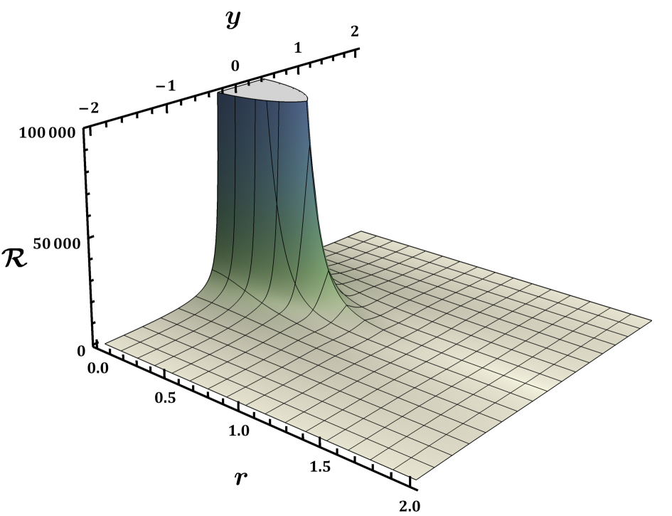
(a)

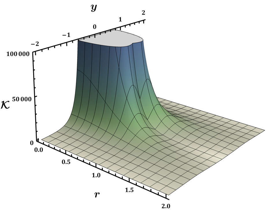
(b)

Figure 3: (a) The invariant quantity $\mathcal{R}\equiv R_{MN}R^{MN}$ in terms of the coordinates $(r,y)$ for $k=1$, $M=10$, $Q=1$, and $\Lambda=5\times 10^{-4}$, and (b) the invariant quantity $\mathcal{K}\equiv R_{MNKL}R^{MNKL}$ for the same values of the parameters.

In order to discuss further the topology of the five-dimensional spacetime (2.7), let us also re-write it in terms of the original non-spherical coordinates $(r,y)$. Employing again the inverse transformations (2.6), the line-element takes the form

$$ds^{2}=e^{-2k|y|} \left\{-f(r,y)dt^{2}+\frac{dr^{2}}{r^{2}+z^{2}(y)}\biggl{[}\frac{r^{2}}{f(r,y)}+z^{2}(y)\biggr{]}+r^{2}d\Omega_{2}^{2}+\frac{2rz(y)\,e^{k|y|}}{r^{2}+z^{2}(y)}\biggl{[}\frac{1}{f(r,y)}-1\biggr{]}drdy\right\}$$

$$\hskip 6.99997pt+\frac{dy^{2}}{r^{2}+z^{2}(y)}\left[r^{2}+\frac{z^{2}(y)}{f(r,y)}\right]\,,$$ (2.11)

where $z(y)=sgn(y)(e^{k|y|}-1)/k$, and

$$f(r,y)=1-\frac{2M}{\sqrt{r^{2}+z^{2}(y)}}+\frac{Q^{2}}{r^{2}+z^{2}(y)}-\frac{\Lambda}{3}\big{[}r^{2}+z^{2}(y)\big{]}\,.$$ (2.12)

As a side remark, we note that the line-element (2) has come out to have the exact same structure as the one employed in [61] for the numerical construction of a 5-dimensional black hole localised on the brane. In our case though all metric components are analytically known whereas, in [61], the five unknown metric fuctions had to be numerically determined.

Returning to the topology of our five-dimensional solution, we are interested in the behaviour of the black-hole horizon(s) in the bulk. If the aforementioned spacetime describes a regular, localised-on-the-brane black hole, its horizon(s) are expected to extend into the bulk but stay close to the brane. To investigate this, we will study the causal structure of the bulk spacetime as this is defined by the light cone. We will consider radial null trajectories in the five-dimensional background (2), and thus keep $\theta$ and $\phi$ constant. Then, for a fixed value $y=y_{0}$ of the fifth coordinate, the condition $ds^{2}=0$ leads to the result

$$\frac{dt}{dr}=\pm\frac{1}{f(r,y_{0})}\left[\frac{r^{2}k^{2}+f(r,y_{0})\left(e^{k|y_{0}|}-1\right)^{2}}{r^{2}k^{2}+\left(e^{k|y_{0}|}-1\right)^{2}}\right]^{1/2},$$ (2.13)

where

$$f(r,y_{0})=1-2M\left[r^{2}+\frac{\left(e^{k|y_{0}|}-1\right)^{2}}{k^{2}}\right]^{-\frac{1}{2}}+Q^{2}\left[r^{2}+\frac{\left(e^{k|y_{0}|}-1\right)^{2}}{k^{2}}\right]^{-1}-\frac{\Lambda}{3}\left[r^{2}+\frac{\left(e^{k|y_{0}|}-1\right)^{2}}{k^{2}}\right].$$ (2.14)

The location and topology of the horizons characterising the line-element (2) may be obtained via Eq. (2.13), by determining the values of $(r,y_{0})$ for which $dt/dr=\pm\infty$, or equivalently $f(r,y_{0})=0$. For $y_{0}=0$, Eq. (2.14) reduces to the metric function $f(r)$ of a four-dimensional Reissner-Nordström-(anti-)de Sitter spacetime for which the emergence and location of horizons has been extensively studied (see, for example, [86, 87]). A similar analysis may be conducted also in the context of the five-dimensional spacetime (2), where the location of horizons is determined by the equation $f(\rho)=0$, with the bulk radial coordinate being $\rho=\sqrt{r^{2}+z^{2}(y)}$ —we keep the $y$-coordinate fixed in Eqs. (2.13) and (2.14) in order to present the view of a static “observer” located at different slices of the bulk spacetime as we move away from the brane.

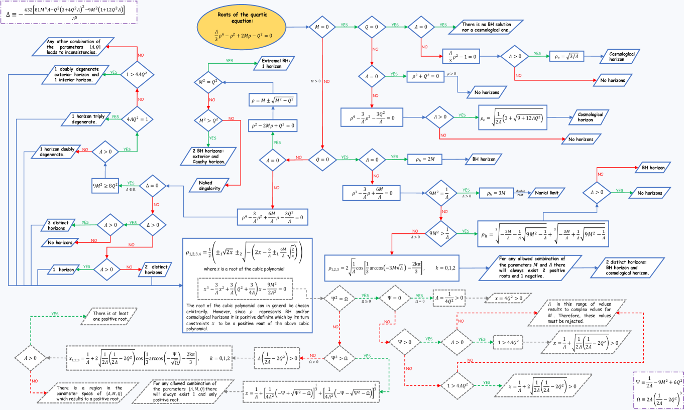
Figure 4: All possible roots of the quartic polynomial $f(\rho)=1-\frac{2M}{\rho}+\frac{Q^{2}}{\rho^{2}}-\frac{\Lambda}{3}\rho^{2}$. In the above flowchart, we catalogue the maximum possible number of horizons for each particular case.

In Fig. 4, we depict a flowchart which constitutes an attentive scrutiny of the roots of the quartic polynomial $f(\rho)=1-\frac{2M}{\rho}+\frac{Q^{2}}{\rho^{2}}-\frac{\Lambda}{3}\rho^{2}$. Every real, positive root of this polynomial corresponds either to a black-hole or a cosmological horizon of the five-dimensional spacetime (2.7). Let us consider some indicative cases. For $M\neq 0$ but $Q=0$ and $\Lambda=0$, we obtain the case of a five-dimensional spacetime with a sole black-hole horizon at $\rho_{H}=2M$. This may be written in terms of $(r,y)$ as

$$r_{H}^{2}=4M^{2}-\frac{\big{(}e^{k|y_{0}|}-1\big{)}^{2}}{k^{2}}\,.$$ (2.15)

This case was studied in [85] where it was shown that the black-hole horizon was exponentially localised close to the brane. Indeed, the aforementioned equation reveals the exponential decrease of $r_{H}$ as $|y_{0}|$ increases and the existence of a value where the horizon vanishes, namely at $|y_{0}|=\ln(2Mk+1)/k$. Beyond this point, any $y$-slice of the five-dimensional spacetime is horizon-free and almost pure AdS, as was shown in [85]. In addition, the black-hole singularity was strictly localised on the brane as in the present analysis.

Does the horizon exponential localisation persist also in the case of multiple horizons? Let us consider the case with $M\neq 0$ and $Q\neq 0$ ($M^{2}>Q^{2}$), but $\Lambda=0$ for simplicity. In that case, it is easy to see that two horizons emerge, an internal Cauchy horizon and an external event horizon located at $\rho_{\pm}=M\pm\sqrt{M^{2}-Q^{2}}$. Employing again the $(r,y)$ coordinates, these are re-written as

$$r_{\pm}^{2}=\left(M\pm\sqrt{M^{2}-Q^{2}}\right)^{2}-\frac{\big{(}e^{k|y_{0}|}-1\big{)}^{2}}{k^{2}}\,.$$ (2.16)

We observe that both horizons shrink as we move to $y$-slices of the bulk spacetime located further away from the brane. Once again both horizons cease to exist beyond a certain value of $y$, namely at the values

$$|y_{0}|_{\pm}=\frac{1}{k}\,\ln\left[1+kM\left(1\pm\sqrt{1-\frac{Q^{2}}{M^{2}}}\right)\right]\,.$$ (2.17)

Note that each horizon will vanish at its own value of the $y$-coordinate and that the horizon corresponding to the smaller value of the radial coordinate $\rho$, i.e to the smaller root of the equation $f(\rho)=0$, will vanish first.

The most general case arises when $M\neq 0$, $Q\neq 0$ and $\Lambda>0$. Then, we can have at most three real, positive roots of the equation $f(\rho)=0$, and thus three horizons: an internal Cauchy horizon $\rho_{-}$, an external event horizon $\rho_{+}$ and a cosmological horizon $\rho_{\scriptscriptstyle{C}}$. Their location in terms of the radial coordinate $\rho$ is determined solely by the parameters $M$, $Q$ and $\Lambda$ and they naturally extend both on the brane and in the bulk. As above, their profile in the bulk may be studied if we change to the $(r,y)$ coordinates; then, the following general relation holds

$$r_{h}^{2}=\rho_{h}^{2}-\frac{\big{(}e^{k|y_{0}|}-1\big{)}^{2}}{k^{2}}\,,$$ (2.18)

where the subscript $h$ has been used to denote the location of all three horizons. Since the value of $\rho_{h}$ is fixed by $M$, $Q$ and $\Lambda$, it is obvious that as $|y_{0}|$ increases the value of $r_{h}$ exponentially decreases. Thus, as we move along the extra dimension away from the brane, $r_{h}$ quickly shrinks and becomes zero at a distance

$$|y_{0}|_{(h)}=\frac{1}{k}\ln(k\rho_{h}+1)\,.$$ (2.19)

Again, each horizon will vanish at a different point along the extra dimension: the Cauchy horizon will vanish first, the event horizon will follow next and the cosmological horizon will disappear last. Due to the exponential fall-off of each $r_{h}$ in terms of the $y$-coordinate, all horizons acquire a “pancake” shape with its longer dimension lying along the brane and its shorter one along the bulk. As an indicative case, in Fig. 5 we give the geometrical representation of the event horizon of the five-dimensional Schwarzschild spacetime. It is important to stress that by introducing non-vanishing $Q$ or $\Lambda$ the depicted general behaviour does not change.

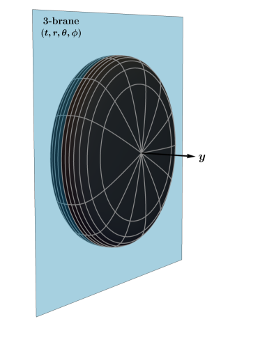
(a)

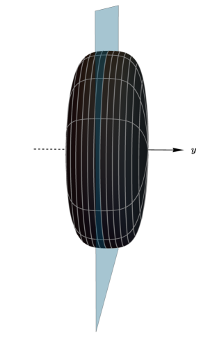
(b)         

Figure 5: The horizon of the localized five-dimensional Schwarzschild black-hole from the bulk point of view for $M=7$, $k=0.5$, $Q=0$ and $\Lambda=0$. Both figures (a) and (b) depict the same image from different angles. The depicted brane coordinates are the radial coordinate $r$ and the angular coordinate $\phi$.

3 The Gravitational Theory

After constructing the geometrical set-up of our five-dimensional gravitational theory, we now consider its action functional which is described by the general expression

$$S_{B}=\int d^{5}x\,\sqrt{-g}\left(\frac{R}{2\kappa_{5}^{2}}+\mathcal{L}^{(B)}_{m}\right).$$ (3.1)

In the above, $R$ is the Ricci scalar constructed in terms of the metric tensor $g_{MN}$ of the five-dimensional spacetime, and $\kappa_{5}^{2}=8\pi G_{5}$ incorporates the five-dimensional gravitational constant $G_{5}$. All matter fields, which may exist in the bulk, are described by the Lagrangian density $\mathcal{L}^{(B)}_{m}$. Notice that we have not explicitly included the five-dimensional cosmological constant $\Lambda_{5}$ in the above action – as we will see in the analysis below, this quantity will appear naturally inside the bulk energy-momentum tensor.

By varying the aforementioned action functional $S_{B}$ with respect to the metric tensor $g_{MN}$, we may derive the gravitational field equations in the bulk which have the form

$$G_{MN}=\kappa_{5}^{2}\,T^{(B)}_{MN}\,.$$ (3.2)

The quantity $G_{MN}=R_{MN}-\frac{1}{2}\,g_{MN}R$ denotes the Einstein-tensor while

$$T^{(B)}_{MN}=-\frac{2}{\sqrt{-g}}\frac{\delta\left(\mathcal{L}^{(B)}_{m}\sqrt{-g}\right)}{\delta g^{MN}}$$ (3.3)

is the bulk energy-momentum tensor associated with the Lagrangian density $\mathcal{L}^{(B)}_{m}$. If we use the gravitational background (2.7) constructed in the previous section, we find that the non-zero components of $T^{(B)}_{MN}$ in mixed form are the following:

$$T^{(B)t}{}_{t}=T^{(B)\rho}{}_{\rho}=\frac{1}{\kappa_{5}^{2}}\left[2(3k^{2}-\Lambda)+\frac{3k\cos\chi}{\rho^{2}}\left(3M-\frac{2Q^{2}}{\rho}\right)-\frac{3M}{\rho^{3}}\right],$$ (3.4)

$$T^{(B)\chi}{}_{\chi}=T^{(B)\theta}{}_{\theta}=T^{(B)\phi}{}_{\phi}=\frac{1}{\kappa_{5}^{2}}\left[2(3k^{2}-\Lambda)-\frac{6k^{2}\cos^{2}\chi}{\rho}\left(M-\frac{Q^{2}}{\rho}\right)+\frac{6kM\cos\chi}{\rho^{2}}\right].$$ (3.5)

The bulk energy-momentum tensor is thus characterized solely by three components: the energy-density $\rho_{E}\equiv-T^{(B)t}{}_{t}$, the radial pressure $p_{1}\equiv T^{(B)\rho}{}_{\rho}$, and a common tangential pressure $p_{2}\equiv T^{(B)\chi}{}_{\chi}=T^{(B)\theta}{}_{\theta}=T^{(B)\phi}{}_{\phi}$. Therefore, the gravitational background (2.7) of a five-dimensional, localised close to the brane black-hole solution may be supported by a diagonal energy-momentum tensor which describes an anisotropic fluid. Employing the fluid’s timelike five-velocity $U^{M}$ and a spacelike unit vector in the direction of $\rho$-coordinate satisfying the relations

$$U^{M}=\{U^{t},0,0,0,0\},\hskip 10.00002ptU^{M}U^{N}g_{MN}=-1\,,$$ (3.6)

$$X^{M}=\{0,X^{\rho},0,0,0\},\hskip 10.00002ptX^{M}X^{N}g_{MN}=1\,,$$ (3.7)

the bulk energy-momentum tensor may be written in a covariant notation as follows

$$T^{(B)MN}=(\rho_{E}+p_{2})U^{M}U^{N}+(p_{1}-p_{2})X^{M}X^{N}+p_{2}\,g^{MN}\,.$$ (3.8)

The aforementioned, rather minimal, content of the bulk energy-momentum tensor was first found in the case where the brane background was assumed to be the Schwarzschild solution [85]. As we see, this structure persists also in the case where the brane background assumes the form of more generalised four-dimensional black-hole solutions.

In fact, there are only two independent components of the energy-momentum tensor, namely the energy-density $\rho_{E}$ and the tangential pressure component $p_{2}$; as Eq. (3.4) reveals, the radial pressure component $p_{1}$ is found to satisfy the equation of state $p_{1}=-\rho_{E}$ everywhere in the bulk. In addition, at asymptotic infinity, i.e. as $\rho\rightarrow+\infty$, all three components of the energy-momentum tensor reduce to a constant value, which can be identified as the five-dimensional cosmological constant $\Lambda_{5}$,

$$\lim_{\rho\rightarrow+\infty}\rho_{E}(\rho,\chi)=-\frac{2(3k^{2}-\Lambda)}{\kappa_{5}^{2}}\equiv\Lambda_{5}\,,$$ (3.9)

$$\lim_{\rho\rightarrow+\infty}p_{1}(\rho,\chi)=\lim_{\rho\rightarrow+\infty}p_{2}(\rho,\chi)=\frac{2(3k^{2}-\Lambda)}{\kappa_{5}^{2}}\equiv-\Lambda_{5}\,.$$ (3.10)

As discussed in the previous section and also confirm here, the asymptotic form of the bulk spacetime depends on the sign of the quantity $(3k^{2}-\Lambda)$. If $3k^{2}>\Lambda$, the asymptotic form of the energy-momentum tensor reduces to that of a negative bulk cosmological constant and the curvature invariant quantities $R$, $\mathcal{R}$, $\mathcal{K}$ match the ones of an AdS₅ spacetime. Then, the brane parameter $\Lambda$ is determined through the relation $2\Lambda=6k^{2}-\kappa^{2}_{5}|\Lambda_{5}|$, and its exact value depends on the inter-balance between the warp parameter $k$ and the bulk cosmological constant $\Lambda_{5}$. In the special case where a fine-tuning is imposed so that $\Lambda=0$, the metric (2.7) incorporates exactly the Randall-Sundrum model [8, 9] at the spacetime boundary. Note, however, that the form of the warp factor remains of an exponential form, i.e. $e^{-k|y|}$, in our analysis regardless of the value of $\Lambda$.

(a)

(b)

Figure 6: (a) The profiles of the energy density $\rho_{E}$ and tangential pressure $p_{2}$ in terms of the $y$-coordinate for $\kappa_{5}=1$, $k=1$, $M=10$, $Q=9$, $\Lambda=5\times 10^{-21}$ and $r=0.85$. (b) The profiles of $T^{(B)r}{}_{r}$, $T^{(B)r}{}_{y}$, $T^{(B)y}{}_{r}$ and $T^{(B)y}{}_{y}$ depicted for the same values of the parameters. Region I lies inside the Cauchy horizon, region II corresponds to the bulk spacetime between the two black-hole horizons, while region III is located between the exterior black-hole horizon and the cosmological one.

In order to study in more detail the profiles of the energy density $\rho_{E}$ and pressure $p_{2}$ in the bulk, we employ again the coordinates $(r,y)$. Using Eqs. (2.6), (3.4) and (3.5), we find

$$\rho_{E}(r,y)=-\frac{1}{\kappa_{5}^{2}}\left\{2(3k^{2}-\Lambda)-\frac{3Mk^{3}\left(4-3e^{k|y|}\right)}{\left[k^{2}r^{2}+\left(e^{k|y|}-1\right)^{2}\right]^{3/2}}-\frac{6Q^{2}k^{4}\left(e^{k|y|}-1\right)}{\left[k^{2}r^{2}+\left(e^{k|y|}-1\right)^{2}\right]^{2}}\right\}\,,$$ (3.11)

$$p_{2}(r,y)=\frac{1}{\kappa_{5}^{2}}\left\{2(3k^{2}-\Lambda)+\frac{6Mk^{3}\left(e^{k|y|}-1\right)\left(2-e^{k|y|}\right)}{\left[k^{2}r^{2}+\left(e^{k|y|}-1\right)^{2}\right]^{3/2}}+\frac{6Q^{2}k^{4}\left(e^{k|y|}-1\right)^{2}}{\left[k^{2}r^{2}+\left(e^{k|y|}-1\right)^{2}\right]^{2}}\right\}\,.$$ (3.12)

In Fig. 6(6(a)), we present the profiles of the energy density $\rho_{E}$ and tangential pressure $p_{2}$ in terms of the bulk coordinate $y$. In this indicative case, the values of the parameters were chosen to be $\kappa_{5}=1$, $k=1$, $M=10$, $Q=9$, $\Lambda=5\times 10^{-21}$, and we have also fixed the radial coordinate on the brane at the random value $r=0.85$. Substituting the aforementioned values of $M$, $Q$ and $\Lambda$ in the flowchart of Fig. 4, one can evaluate the locations of the three distinct horizons, namely $\rho_{-}=5.64$ (Cauchy horizon), $\rho_{+}=14.36$ (exterior black-hole horizon) and $\rho_{\scriptscriptstyle{C}}=2.45\times 10^{10}$ (cosmological horizon). Given these values and the fixed radial distance $r=0.85$, it is straightforward to calculate from Eq. (2.18) the corresponding values of $y$ at which we encounter the three horizons in the bulk: the Cauchy horizon lies at $y_{-}=1.88$, the exterior black-hole horizon at $y_{+}=2.73$, and the cosmological horizon at $y_{c}=23.92$. We denote the bulk region inside the Cauchy horizon as region I, the region between the two black-hole horizons as region II, and the region between the exterior black-hole horizon and the cosmological horizon as region III; we denote these regions also in Fig. 6(6(b)).

We observe that both the energy density $\rho_{E}$ and tangential pressure $p_{2}$ exhibit a shell-like distribution in region I, i.e. in the region between the brane, located at $y=0$, and the Cauchy horizon. As the latter is approached, both components quickly decrease towards their AdS₅ asymptotic values given by Eqs. (3.9) and (3.10). These values are adopted even before the exterior black-hole horizon is reached, therefore, as Fig. 6(6(a)) clearly depicts, region III describes a pure AdS₅ spacetime. On the brane, the energy density $\rho_{E}$ and tangential pressure $p_{2}$ adopt values which respect all energy conditions since there we have $\rho_{E}>0$, $\rho_{E}+p_{1}=0$ and $\rho_{E}>p_{2}$. Although the profiles of $\rho_{E}$ and $p_{2}$ depend on the chosen values of the parameters of the theory, the behaviour depicted in Fig. 6(6(a)) is by no means a special one and in fact arises for a large number of sets of parameter values. What we should also stress is the emergence of a regime close to the Cauchy horizon where the energy conditions are violated since $\rho_{E}<p_{2}$. The same behaviour was also observed in our previous work [85] and seems to be a requisite for the localisation of the black-hole topology close to the brane as well as for the transition to a pure AdS₅ spacetime which, by construction, is characterised by the relation $p_{i}=-\rho_{E}=|\Lambda_{5}|$.

When we perform the coordinate change described via Eq. (2.6), the components $T^{(B)M}{}_{N}$ of the energy-momentum tensor are bound to change. The $T^{(B)t}{}_{t}\equiv-\rho_{E}$ and $T^{(B)\theta}{}_{\theta}=T^{(B)\phi}{}_{\phi}\equiv p_{2}$ components receive no additive corrections and their change amounts to merely substituting $\{\rho,\chi\}$ by $\{r,y\}$ in their expressions, thus leading to Eqs. (3.11) and (3.12). However, the $T^{(B)r}{}_{r}$, $T^{(B)r}{}_{y}$, $T^{(B)y}{}_{r}$ and $T^{(B)y}{}_{y}$ components receive also additive corrections and their expressions are significantly modified. The analysis leading to the new expressions of all the components of the energy-momentum tensor is given in Appendix C. Therefore, for completeness, in Fig. 6(6(b)) we depict also the behaviour of these four components of the energy-momentum tensor in terms of the extra dimension $y$ and for the same set of parameter values as in Fig. 6(6(a)). As was the case with $\rho_{E}$ and $p_{2}$, these components remain everywhere regular, have a shell-like distribution inside region I and quickly adopt their asymptotic values even before the exterior black-hole horizon is reached: for the $T^{(B)r}{}_{r}$ and $T^{(B)y}{}_{y}$ components, this asymptotic value is $|\Lambda_{5}|$ while, for the off-diagonal components $T^{(B)r}{}_{y}$ and $T^{(B)y}{}_{r}$, this asymptotic value is zero, as expected. Note also that the coordinate change (2.6) destroys the simple relations (3.4), (3.5) between the components of the energy momentum tensor which were valid in the $\{t,\rho,\chi,\theta,\phi\}$ set of coordinates. All these reveal that, although the “axial” set of coordinates $\{t,r,\theta,\phi,y\}$ serve better to illustrate the behaviour of both the curvature and distribution of matter with respect to the brane observer, it is the “spherical” set of coordinates $\{t,\rho,\chi,\theta,\phi\}$ which encodes the highest symmetry of the five-dimensional theory and leads to the simplest profile of both the spacetime and the energy-momentum tensor.

3.1 A Field-Theory Toy-Model

In this subsection, we will investigate further the nature of the bulk energy-momentum tensor which is necessary to support the geometry of the five-dimensional localized Reissner-Nordström-(A)dS black hole presented in Section 2. Due to the simple structure of $T_{MN}^{(B)}$, given in Eqs. (3.4), (3.5), the term “anisotropic fluid” was used to describe it, and a covariant form for its expression was also found. However, it would be interesting to see if a field-theory model could be proposed to support it, and under which conditions on the associated fields this task could be fulfilled.

In the following analysis, we will use the spherically-symmetric set of coordinates $\{t,\rho,\chi,\theta,\phi\}$ in which $T^{(B)}_{MN}$ takes its simplest possible form, as argued above. We will employ five-dimensional fields that are allowed to propagate outside our brane, and thus consider scalar or gauge fields which are distinct from the corresponding Standard-Model degrees of freedom living on the brane. According to our results, a theory with only minimally-coupled scalars or with only minimally-coupled vector fields fails to lead to the desired structure of the bulk energy-momentum tensor. We therefore consider a tensor-vector-scalar five-dimensional field theory where the bulk matter Lagrangian density $\mathcal{L}^{(B)}_{m}$ appearing in Eq. (3.1) is given by

$$\mathcal{L}^{(B)}_{m}:=\mathcal{L}^{(g)}+\mathcal{L}^{(sc)}\,,$$ (3.13)

with

$$\mathcal{L}^{(g)}:=-\frac{1}{4}\,F^{MN}F_{MN}\,,$$ (3.14)

$$\mathcal{L}^{(sc)}:=-f_{1}(\xi,\psi)(\partial\xi)^{2}-f_{2}(\xi,\psi)(\partial\psi)^{2}-V(\xi,\psi)\,.$$ (3.15)

Above, $F_{MN}=\nabla_{M}A_{N}-\nabla_{N}A_{M}$ is the field-strength tensor of an Abelian gauge field $A_{M}$ and $\{\xi(\rho,\chi),\psi(\rho,\chi)\}$ are two scalar fields. In addition, we have introduced two arbitrary functions $f_{1}(\xi,\psi)$ and $f_{2}(\xi,\psi)$ in the kinetic terms of the scalar fields as well as an interaction potential $V(\xi,\psi)$. The variation of $\sqrt{-g}\,\mathcal{L}^{(B)}_{m}$ with respect to $g_{MN}$ leads to the result

$$T^{(B)MN}=T^{(g)MN}+T^{(sc)MN}\,,$$ (3.16)

where

$$T^{(g)MN}=F^{MA}F^{N}{}_{A}-\frac{1}{4}\,g^{MN}F^{AB}F_{AB}\,,$$ (3.17)

and

$$T^{(sc)}_{MN}=2f_{1}(\xi,\psi)\partial_{M}\xi\,\partial_{N}\xi+2f_{2}(\xi,\psi)\partial_{M}\psi\,\partial_{N}\psi+g_{MN}\,\mathcal{L}^{(sc)}\,.$$ (3.18)

In what follows, we will also assume the following configuration for the gauge field-strength tensor

$$\left(F^{MN}\right)=\left(\begin{array}[]{ccccc}0&E_{1}(\rho,\chi)&E_{2}(\rho,\chi)&0&0\\[2.84526pt] -E_{1}(\rho,\chi)&0&0&0&0\\[2.84526pt] -E_{2}(\rho,\chi)&0&0&0&0\\[2.84526pt] 0&0&0&0&B(\rho,\chi,\theta)\\[2.84526pt] 0&0&0&-B(\rho,\chi,\theta)&0\end{array}\right),$$ (3.19)

where $E_{1}$, $E_{2}$ and $B$ stand for two components of the “electric” bulk gauge field and a sole component of the “magnetic” field, respectively. Employing the above in Eq. (3.17), one may easily calculate the components of the gauge-field energy-momentum tensor $T^{(g)MN}$. Using also the expression (3.18), the components of $T^{(sc)}_{MN}$ for the two scalar fields readily follow. Taking their sum, we obtain the following results for the non-vanishing mixed components of the bulk energy-momentum tensor

$$T^{(B)t}{}_{t}=\frac{1}{2}(-bB^{2}+a_{1}E_{1}^{2}+a_{2}E_{2}^{2})-f_{1}(\partial\xi)^{2}-f_{2}(\partial\psi)^{2}-V,$$

$$T^{(B)\rho}{}_{\rho}=\frac{1}{2}(-bB^{2}+a_{1}E_{1}^{2}-a_{2}E_{2}^{2})+f_{1}\left(\partial^{\rho}\xi\partial_{\rho}\xi-\partial^{\chi}\xi\partial_{\chi}\xi\right)+f_{2}\left(\partial^{\rho}\psi\partial_{\rho}\psi-\partial^{\chi}\psi\partial_{\chi}\psi\right)-V,$$

$$T^{(B)\rho}{}_{\chi}=a_{2}E_{1}E_{2}+2\left(f_{1}\,\partial^{\rho}\xi\partial_{\chi}\xi+f_{2}\,\partial^{\rho}\psi\partial_{\chi}\psi\right),$$ (3.20)

$$T^{(B)\chi}{}_{\chi}=\frac{1}{2}(-bB^{2}-a_{1}E_{1}^{2}+a_{2}E_{2}^{2})-f_{1}\left(\partial^{\rho}\xi\partial_{\rho}\xi-\partial^{\chi}\xi\partial_{\chi}\xi\right)-f_{2}\left(\partial^{\rho}\psi\partial_{\rho}\psi-\partial^{\chi}\psi\partial_{\chi}\psi\right)-V,$$

$$T^{(B)\theta}{}_{\theta}=T^{(B)\phi}{}_{\phi}=\frac{1}{2}(bB^{2}-a_{1}E_{1}^{2}-a_{2}E_{2}^{2})-f_{1}(\partial\xi)^{2}-f_{2}(\partial\psi)^{2}-V.$$

In the above, we have defined the quantities $a_{1}\equiv g_{tt}\,g_{\rho\rho}$, $a_{2}\equiv g_{tt}\,g_{\chi\chi}$ and $b\equiv g_{\theta\theta}\,g_{\phi\phi}$ for simplicity.

Let us now investigate whether the above set of components can be simplified in order to resemble the minimal configuration described by Eqs. (3.4), (3.5). We thus first demand that $T^{(B)t}{}_{t}=T^{(B)\rho}{}_{\rho}$, and we obtain the constraint

$$E_{2}^{2}=\frac{2\left(f_{1}\,\partial^{\rho}\xi\partial_{\rho}\xi+f_{2}\,\partial^{\rho}\psi\partial_{\rho}\psi\right)}{a_{2}}\,.$$ (3.21)

We next observe that the configuration of Eqs. (3.4), (3.5) has no off-diagonal component. Thus demanding that $T^{(B)\rho}{}_{\chi}=0$ and employing Eq. (3.21), we also obtain

$$E_{1}^{2}=\frac{1}{a_{2}}\frac{2\left(f_{1}\,\partial^{\rho}\xi\partial_{\chi}\xi+f_{2}\,\partial^{\rho}\psi\partial_{\chi}\psi\right)^{2}}{f_{1}\,\partial^{\rho}\xi\partial_{\rho}\xi+f_{2}\,\partial^{\rho}\psi\partial_{\rho}\psi}\,.$$ (3.22)

Demanding finally that $T^{(B)\chi}{}_{\chi}=T^{(B)\theta}{}_{\theta}=T^{(B)\phi}{}_{\phi}$, we are led to a third constraint

$$B^{2}=\frac{2\left[f_{1}(\partial\xi)^{2}+f_{2}(\partial\psi)^{2}\right]}{b}\,.$$ (3.23)

Therefore, the co-existence in the bulk of the three components of the field-strength tensor with the two scalar fields, in a way that they satisfy the above three constraints, ensures that the total energy-momentum tensor in the bulk acquires the form dictated by Eqs. (3.4), (3.5).

In addition, setting $\rho_{E}\equiv-T^{(B)t}{}_{t}$ and $p_{2}\equiv T^{(B)\chi}{}_{\chi}$, the remaining two components give

$$f_{1}(\partial\xi)^{2}+f_{2}(\partial\psi)^{2}+V=\frac{1}{2}(\rho_{E}-p_{2})\,,$$ (3.24)

$$bB^{2}-a_{1}E_{1}^{2}-a_{2}E_{2}^{2}=\rho_{E}+p_{2}\,.$$ (3.25)

Therefore, the two independent components of the energy-momentum tensor in the bulk are determined by the exact profiles of the gauge and scalar fields. These in turn must satisfy their own equations of motion. By considering the variation of the action $S_{B}$ with respect to $A_{M}$, we obtain the five-dimensional equation for the gauge field in the bulk, namely

$$\partial_{M}\left(\sqrt{-g}\,F^{MN}\right)=0\,.$$ (3.26)

Considering the components $N=t$ and $N=\phi$, we find

$$\displaystyle{\partial_{\rho}E_{1}+\partial_{\chi}E_{2}+E_{1}\frac{\partial_{\rho}\sqrt{-g}}{\sqrt{-g}}+E_{2}\frac{\partial_{\chi}\sqrt{-g}}{\sqrt{-g}}=0}\,,$$ (3.27)

$$\partial_{\theta}B+\frac{B\,\cos\theta}{\sin\theta}=0\Rightarrow B(\rho,\chi,\theta)=\frac{B_{0}(\rho,\chi)}{\sin\theta}\,,$$ (3.28)

respectively, while the remaining components are identically zero. Additionally, the variation of $S_{B}$ with respect to the scalar fields $\xi$ and $\psi$ results in the equations

$$\frac{1}{2}\left[(\partial_{\xi}f_{1})(\partial\xi)^{2}+(\partial_{\xi}f_{2})(\partial\psi)^{2}+\partial_{\xi}V\right]=\frac{\partial_{M}\left(\sqrt{-g}\,f_{1}\,g^{MN}\partial_{N}\xi\right)}{\sqrt{-g}}\,,$$ (3.29)

$$\frac{1}{2}\left[(\partial_{\psi}f_{1})(\partial\xi)^{2}+(\partial_{\psi}f_{2})(\partial\psi)^{2}+\partial_{\psi}V\right]=\frac{\partial_{M}\left(\sqrt{-g}\,f_{2}\,g^{MN}\partial_{N}\psi\right)}{\sqrt{-g}}\,.$$ (3.30)

The above set of four differential equations (3.27)-(3.30), together with the constraints (3.22)-(3.25), may indeed possess a mathematically consistent solution. The complexity of the system would most likely demand numerical calculation for this solution to be derived. However, instead of attempting to solve this coupled system of equations, we would like to examine the ensuing characteristics of the fields. To this end, let us focus on Eq. (3.25): employing the exact form of the components $\rho_{E}$ and $p_{2}$ from Eqs. (3.4), (3.5), we may rewrite it as

$$bB^{2}-a_{1}E_{1}^{2}-a_{2}E_{2}^{2}=\frac{1}{\kappa_{5}^{2}}\left[-\frac{6k^{2}\cos^{2}\chi}{\rho}\left(M-\frac{Q^{2}}{\rho}\right)-\frac{3k\cos\chi}{\rho^{2}}\left(3M-\frac{2Q^{2}}{\rho}\right)+\frac{3M}{\rho^{3}}\right].$$ (3.31)

The right-hand-side of the above equation is clearly not sign-definite. For small $\rho$, it is positive definite since in this regime both $\rho_{E}$ and $p_{2}$ are positive, as Fig. 6(6(a)) reveals. However, as $\rho$ increases, negative-valued terms inside the square brackets begin to dominate making this combination clearly negative for large values of $\rho$. Since $a_{1}<0$, $a_{2}<0$ and $b>0$, according to their definitions below Eq. (3.20), this means that at least one of the components of the gauge field strength-tensor $F_{MN}$ must turn imaginary near the bulk boundary. Due to the constraints (3.22), (3.23), this may lead to $\xi$ or $\psi$ also becoming imaginary.

Simpler variants of the above model may also be built, however, they all suffer from the above problem. For instance, if we consider the case with $E_{2}=0$ and $\xi=\xi(\chi)$ together with the condition $f_{2}=0$, the energy-momentum tensor comes out to be automatically diagonal and satisfying $T^{(B)t}{}_{t}=T^{(B)\rho}{}_{\rho}$. The constraints (3.21), (3.22) now disappear while the one for $B$ still holds. The gauge-field equations (3.27) and (3.28) are easily satisfied for a wide range of choices for $E_{1}$ and $B$. The second scalar field $\psi(\rho,\chi)$ is now an auxilary field whose equation of motion (3.30) introduces a constraint between $f_{1}$ and $V$. Nevertheless, Eq. (3.31) still holds with $E_{2}=0$, and thus the necessity for a “phantom” gauge field (and a “phantom” scalar field) at the bulk boundary still exists.

Phantom scalar fields are often used in the context of four-dimensional analyses as a mean to create the necessary yet peculiar dark energy component with $w<-1$ in our universe. In our analysis, a bulk matter with also peculiar characteristics seems to be necessary to localise a five-dimensional black hole on the brane, otherwise its singularity would leak in the bulk. The desired structure of the bulk energy-momentum tensor as well as the introduction of the “charge” parameter $Q$ in our metric demand the presence of gauge and scalar fields with phantom-like properties at the bulk boundary. We should stress that all fields are “ordinary” close to our brane and no violation of energy conditions takes place on our brane. Could a gauge field, that turns phantom-like at the outskirts of the bulk spacetime, be considered as “natural” or at least acceptable? Such an analysis, although well-motivated, would take us beyond the scope of the present study and is thus left for a future work.

4 Junction Conditions and Effective Theory

In this final section, we turn our attention from the structure and content of the five-dimensional spacetime to issues related to the presence of the brane itself, namely its consistent embedding in the bulk and the effective four-dimensional gravitational equations. A detailed derivation of the effective theory on the 3-brane in brane-world models was presented in [88], however, in order to keep our analysis self-contained, we will reproduce here the main results and equations. It is also important to note that in [88] the bulk matter of the brane-world model was described only by a negative cosmological constant, whereas in our case the bulk spacetime contains an anisotropic fluid, a feature that slightly modifies some parts of the analysis.

In the standard brane-world scenario, our 3-brane ($\Sigma$, $h_{MN}$) is embedded in the five-dimensional spacetime ($\mathcal{M}$, $g_{MN}$) at $y=0$. The induced metric on the brane is defined via the relation $h_{MN}\equiv\left(g_{MN}\right)_{y=0}-n_{M}n_{N}$, where $n^{M}$ is the unit normal vector to the 3-brane. From Eq. (2), we may deduce that $n^{M}=\delta^{M}{}_{y}$. In what follows, we will denote tensors on $\Sigma$ with a bar to be distinguished from the corresponding five-dimensional tensors. Using the Gauss’s Theorema Egregium

$$\bar{R}^{A}{}_{BCD}=h^{A}{}_{M}\,h^{N}{}_{B}\,h^{K}{}_{C}\,h^{L}{}_{D}R^{M}{}_{NKL}+2K^{A}{}_{[C}K_{D]B}\,,$$ (4.1)

and the Codazzi’s equation

$$R_{AB}\,h^{A}{}_{M}\,n^{B}=D_{L}K^{L}{}_{M}-D_{M}\,K\,,$$ (4.4)

we obtain the following relation for the Einstein tensor on the 3-brane:

$$\bar{G}_{MN}=h^{A}{}_{M}h^{B}{}_{N}\,G_{AB}+R_{AB}\,n^{A}n^{B}h_{MN}+KK_{MN}-K_{M}{}^{L}K_{LN}-\frac{1}{2}h_{MN}\left(K^{2}-K^{AB}K_{AB}\right)-\widetilde{E}_{MN}\,.$$ (4.5)

In the above, $K_{MN}$ is the extrinsic curvature of the brane defined as

$$K_{MN}\equiv h^{A}{}_{M}\,h^{B}{}_{N}\,\nabla_{A}\,n_{B}=h^{L}{}_{M}\,\nabla_{L}\,n_{N}\,,$$ (4.6)

while

$$\widetilde{E}_{MN}\equiv R^{A}{}_{BCD}\,n_{A}\,n^{C}\,h^{B}{}_{M}\,h^{D}{}_{N}\,.$$ (4.7)

Decomposing the Riemann tensor into the Weyl curvature, the Ricci tensor and the Ricci scalar, we obtain

$$R_{ABCD}=\frac{2}{3}\left(g_{A[C}R_{D]B}-g_{B[C}R_{D]A}\right)-\frac{1}{6}g_{A[C}\,g_{D]B}R+C_{ABCD}\,.$$ (4.8)

Using the five-dimensional gravitational field equations (3.2) together with (4.8) in (4.5) we are led to

$$\bar{G}_{MN}=\frac{2\kappa_{5}^{2}}{3}\left[h^{A}{}_{M}h^{B}{}_{N}\,T^{(B)}_{AB}+\left(n^{A}n^{B}\,T^{(B)}_{AB}-\frac{T^{(B)}}{4}\right)h_{MN}\right]+KK_{MN}-K_{M}{}^{L}K_{LN}$$

$$-\frac{1}{2}h_{MN}\left(K^{2}-K^{AB}K_{AB}\right)-E_{MN}\,,$$ (4.9)

where $T^{(B)}\equiv T^{(B)L}{}_{L}$ is the trace of the bulk energy-momentum tensor, and

$$E_{MN}\equiv C^{A}{}_{BCD}\,n_{A}\,n^{C}\,h^{B}{}_{M}\,h^{D}{}_{N}\,.$$ (4.10)

As is usual in all brane-world scenarios, we may write the total energy-momentum tensor as the sum of the bulk $T^{(B)}_{MN}$ and brane $T^{(br)}_{\mu\nu}$ energy-momentum tensors, namely

$$T_{MN}=T^{(B)}_{MN}+\delta^{\mu}_{M}\delta^{\nu}_{N}\,T^{(br)}_{\mu\nu}\delta(y)\,.$$ (4.11)

The brane energy-momentum tensor can be decomposed further as follows

$$T^{(br)}_{\mu\nu}=-\sigma\,h_{\mu\nu}+\tau_{\mu\nu}\,,$$ (4.12)

where $\sigma$ is the tension of the brane, and $\tau_{\mu\nu}$ encodes all the other possible sources of energy and/or pressure on the brane. A natural question which arises in the context of our analysis is whether the consistent embedding of our brane in the five-dimensional line-element (2) demands the introduction of a non-trivial $\tau_{\mu\nu}$ on the brane.

In order to investigate this, we will study Israel’s junction conditions [89] at $y=0$. These require that

$$[h_{MN}]=0\,,$$ (4.13)

$$[K_{\mu\nu}]=-\kappa_{5}^{2}\left(T^{(br)}_{\mu\nu}-\frac{1}{3}h_{\mu\nu}\,T^{(br)}\right)\,.$$ (4.14)

In the above, the bracket notation for a quantity $X$ simply means

$$[X]=\lim_{y\rightarrow 0^{+}}X-\lim_{y\rightarrow 0^{-}}X=X^{(+)}-X^{(-)}\,.$$ (4.15)

Let us determine first the components of the induced metric on the brane $h_{MN}$. These are found to be

$$(h_{MN})=\left(\begin{array}[]{ccccc}-\left(1-\frac{2M}{r}+\frac{Q^{2}}{r^{2}}-\frac{\Lambda}{3}r^{2}\right)&0&0&0&0\\[2.84526pt] 0&\left(1-\frac{2M}{r}+\frac{Q^{2}}{r^{2}}-\frac{\Lambda}{3}r^{2}\right)^{-1}&0&0&0\\[2.84526pt] 0&0&r^{2}&0&0\\ 0&0&0&r^{2}\sin^{2}\theta&0\\ 0&0&0&0&0\end{array}\right)\,.$$ (4.16)

We may easily see that they indeed satisfy Israel’s first condition. Also, employing these, we may easily determine the components of the extrinsic curvature close to the 3-brane which have the form

$$K_{MN}=-k\frac{d|y|}{dy}\,\delta^{\mu}_{M}\delta^{\nu}_{N}\,h_{\mu\nu}.$$ (4.17)

The trace of $K_{MN}$ is also found to be $K=-4k\,(d|y|/dy)$. We may alternatively write Eq. (4.14) as

$$T^{(br)}_{\mu\nu}=-\frac{1}{\kappa_{5}^{2}}\left([K_{\mu\nu}]-h_{\mu\nu}[K]\right)\,.$$ (4.18)

Using Eq. (4.15), the assumed $\mathbf{Z}_{2}$-symmetry of the model in the bulk and the components of $K_{\mu\nu}$, we find

$$T^{(br)}_{\mu\nu}=-\frac{6k}{\kappa_{5}^{2}}\,h_{\mu\nu}\,.$$ (4.19)

Comparing Eq. (4.19) with Eq. (4.12), we easily deduce that $\sigma=6k/\kappa_{5}^{2}>0$, while $\tau_{\mu\nu}=0$. This means that the consistent embedding of our 3-brane in the five-dimensional spacetime constructed in Section 2—and described by either the line-element (2) or (2.7)—does not demand the introduction of any additional matter on the brane. In the context of the five-dimensional theory, the brane contains only its constant positive self-energy $\sigma$. In fact, it is this quantity together with the five-dimensional gravitational constant $\kappa_{5}^{2}$ that determine the warp parameter $k$ of the line-element in the bulk.

We may now proceed to derive the effective theory on the brane. The gravitational equations on the 3-brane can be determined from Eq. (4.9) by setting $y=0$. We note that for either $M$ or $N$ equal to $y$, the r.h.s. of (4.9) is trivially zero; this implies that $\bar{G}_{yN}=0\ \forall N$, as expected. Due to the $\mathbf{Z}_{2}$-symmetry, we may perform the calculation either on the $+$ or $-$ side of the brane, therefore we will omit the $\pm$ signs in what follows. Using the results for the induced metric $h_{MN}$, the extrinsic curvature $K_{MN}$ and the normal vector $n^{M}$ derived above in (4.12), we obtain

$$\bar{G}_{\mu\nu}=8\pi G_{4}\left(T^{(eff)}_{\mu\nu}+\tau_{\mu\nu}\right)+\kappa_{5}^{4}\left(\pi_{\mu\nu}-\frac{\ \sigma^{2}}{12}\,h_{\mu\nu}\right)-E_{\mu\nu}\Big{|}_{y\rightarrow 0}\,,$$ (4.20)

where

$$G_{4}=\frac{\kappa_{5}^{4}\,\sigma}{48\pi}\,,$$ (4.21)

$$T^{(eff)}_{\mu\nu}\equiv\frac{2}{3k}\left[T^{(B)}_{\mu\nu}+\left(T^{(B)}_{yy}-\frac{T^{(B)}}{4}\right)h_{\mu\nu}\right]_{y=0}\,,$$ (4.22)

$$\pi_{\mu\nu}=-\frac{1}{4}\tau_{\mu}{}^{\lambda}\,\tau_{\lambda\nu}+\frac{1}{12}\tau\,\tau_{\mu\nu}+\frac{1}{8}\tau^{\alpha\beta}\tau_{\alpha\beta}\,h_{\mu\nu}-\frac{1}{24}\tau^{2}\,h_{\mu\nu}\,.$$ (4.23)

In the above, $G_{4}$ constitutes the effective four-dimensional gravitational constant on the brane; this is also defined in terms of the fundamental gravitational constant $\kappa_{5}^{2}$ and the brane tension $\sigma$. The quantity $\pi_{\mu\nu}$ is the well-known quadratic contribution of $\tau_{\mu\nu}$ [88] which here, however, trivially vanishes since $\tau_{\mu\nu}=0$. Finally, $T^{(eff)}_{\mu\nu}$ can be interpreted as the effective energy-momentum tensor on the brane. Together with $E_{\mu\nu}$, they constitute the imprint of the dynamics of the bulk fields—gravitational, and possibly gauge and scalar fields generating the bulk energy-momentum tensor $T^{(B)}_{MN}$—on the brane. The components of $T^{(eff)}_{\mu\nu}$ are given by the following relation

$$T^{(eff)}_{\mu\nu}=\frac{1}{\kappa_{5}^{2}k}\left[3k^{2}h_{\mu\nu}-{\Lambda}\,h_{\mu\nu}+\frac{M}{r^{3}}\left(\begin{array}[]{cccc}-h_{tt}&0&0&0\\ 0&-h_{rr}&0&0\\ 0&0&h_{\theta\theta}&0\\ 0&0&0&h_{\phi\phi}\\ \end{array}\right)\right]\,,$$ (4.24)

while the components of the tensor $E_{\mu\nu}$, defined in (4.10), are evaluated to be

$$E_{\mu}{}_{\nu}\Big{|}_{y\rightarrow 0}=\left(-\frac{Q^{2}}{r^{4}}+\frac{M}{r^{3}}\right)\left(\begin{array}[]{cccc}-h_{tt}&0&0&0\\ 0&-h_{rr}&0&0\\ 0&0&h_{\theta\theta}&0\\ 0&0&0&h_{\phi\phi}\end{array}\right)\,.$$ (4.25)

We notice that $E_{\mu\nu}$ is evaluated infinitesimally close to the brane but not exactly on it, its source being the five-dimensional Weyl tensor. Substituting the above relations in (4.20), we obtain

$$\bar{G}_{\mu\nu}=\left(\begin{array}[]{cccc}\left(\frac{Q^{2}}{r^{4}}+\Lambda_{4}\right)f(r)&0&0&0\\ 0&-\left(\frac{Q^{2}}{r^{4}}+\Lambda_{4}\right)\frac{1}{f(r)}&0&0\\ 0&0&\left(\frac{Q^{2}}{r^{4}}-\Lambda_{4}\right)r^{2}&0\\ 0&0&0&\left(\frac{Q^{2}}{r^{4}}-\Lambda_{4}\right)r^{2}\sin^{2}\theta\end{array}\right)\,,$$ (4.26)

with

$$f(r)\equiv 1-\frac{2M}{r}+\frac{Q^{2}}{r^{2}}-\frac{\Lambda_{4}}{3}r^{2}\,.$$ (4.27)

One can verify that the expression of the Einstein tensor in (4.26) matches exactly the Einstein tensor of the four-dimensional Reissner-Nordström-(A)dS metric, with $\Lambda_{4}=\Lambda$ being the effective cosmological constant on the brane and $Q^{2}/r^{4}$ the equivalent of the energy-momentum tensor component of an electromagnetic field. Although we have called our five-dimensional black-hole solution a Reissner-Nordström-(A)dS one, it is clear that no four-dimensional electromagnetic field has been—or needed to be—introduced on the brane. The “charge” $Q$ is a conserved quantity carried by the bulk fields and left as an imprint in the four-dimensional spacetime. It is therefore a tidal charge, as the one accommodated in the black-hole solution of [21], rather than an ordinary electromagnetic one. It is worth noting that our present analysis can be considered as one which completes the brane black-hole solution found in [21] since it provides the bulk description that was lacking from the aforementioned work.

5 Epilogue

In this work, we have generalised our previous analysis [85], where we studied the localisation of a five-dimensional spherically-symmetric, neutral and asymptotically-flat black hole on our brane, by considering also a cosmological constant and a charge term in the metric function. We have preserved the assumption of spherical symmetry in the five-dimensional bulk and by adopting an appropriate set of spherical coordinates, we have built a black-hole solution with its singularity strictly residing on the brane. We have performed a careful classification of the horizons that this background admits, depending on the values of its parameters, and demonstrated that all of them have pancake shapes and one after the other get exponentially localised close to the brane. The bulk gravitational background is everywhere regular, as the calculation of all scalar gravitational quantities has shown, and reduces to an AdS₅ spacetime right outside the black-hole event horizon. Our analytically constructed, five-dimensional line-element has all the desired geometric features of a physical black hole localised close to our brane, and shares the exact same structure as the line-element employed in [61] where such a solution was numerically constructed.

In order to support such a geometric background, we need to assume the presence of a bulk energy-momentum tensor. In terms of the spherical coordinates, this quantity has a minimal structure: it is diagonal with only two independent components, the energy density $\rho_{E}$ and tangential pressure $p_{2}$, and may be thus described as an anisotropic fluid. Close to and on the brane, both $\rho_{E}$ and $p_{2}$ are positive, and respect all energy conditions. However, in order to localise the black-hole topology close to the brane and prevent the leaking of the singularity along the extra dimension, a transition needs to take place in the bulk resulting in the violation of both the $\rho_{E}\geq 0$ and $\rho_{E}+p_{2}\geq 0$ conditions. This violation is only local and takes place within the event horizon regime in the bulk—soon afterwards, both $\rho_{E}$ and $p_{2}$ reduce to constant quantities, which give rise to the AdS₅ spacetime outside the black-hole event horizon. In fact, a general question emerges from our analysis as to the nature of the necessary bulk matter that is usually asked to satisfy all energy conditions at the location of our brane and, at the same time, to support asymptotically – in the context of most brane-world models – an AdS spacetime which by construction violates most energy conditions. Are there matter or field configurations that would support and smoothly match these two asymptotic behaviours?

To this end, we attempted to provide a physical interpretation of the nature of the bulk matter by building a field-theory model involving scalar and gauge fields living in the bulk. Without determining explicitly the profiles of these fields—a task that would demand numerical analysis, we obtained the primary constraints and equations for a viable solution. Although we demonstrated that this scalar-vector model could indeed reproduce the general structure of the energy-momentum tensor in the bulk, our analysis also revealed that the gauge, and inevitably the scalar, fields should become phantom-like at the bulk boundary. The decision on whether a five-dimensional tensor-scalar-vector theory, whose particle degrees of freedom are well behaved near and on our brane but they turn phantom-like away from it, is physically acceptable is still pending. Alternative field theory constructions could also be considered. For instance, the negative sign of the energy density of the bulk matter points perhaps to a non-minimal gravitational coupling of the fields that takes over at the outskirts of the bulk—the fact that all terms proportional to the charge $Q$, and therefore sourced by the bulk gauge field, remain always positive whereas the gravitational terms proportional to $M$ are the ones that cause the energy density to turn negative seems to agree with this. We plan to study this alternative model in a follow-up work.

By considering the junction conditions, we have subsequently studied in detail the consistent embedding of our 3-brane into the bulk geometry we have constructed. We have demonstrated that no additional matter needs to be introduced on the brane by hand, and that the only energy content of our brane in the context of the five-dimensional theory is its constant , and positive self-energy or tension. In fact it is this quantity together with the five-dimensional gravitational constant that determine the warp parameter of the bulk metric—we note that the warp factor of the model has the exact same form as the one of the original Randall-Sundrum model, a feature which also ensures the localisation of gravity close to our brane. These two fundamental quantities determine also the effective four-dimensional gravitational constant on our brane as the study of the effective theory on the brane revealed. There, we showed that the combined effect of the five-dimensional geometry and the bulk matter leaves its imprint on the brane and supports the Reissner-Nordström-(A)dS geometry that the four-dimensional observer sees. Let us, however, stress again that the charge appearing in the metric is a tidal charge, first employed in the brane construction of [21], rather than an electromagnetic one as it is sourced by the bulk, gravitational and gauge, fields. In this sense, our work provides the description of the bulk geometry which gives rise to the four-dimensional Reissner-Nordström-type of background of [21] and which was missing from that analysis.

Apart from the successful localisation of the black-hole geometry close to our brane and the incorporation of the Randall-Sundrum model in our analysis, our construction supports an Anti-de Sitter spacetime not only at the bulk boundary but effectively throughout the bulk regime outside the black-hole event horizon. Therefore, our results could be considered also in the context of holography [91, 92, 93] and used to study interesting field-theory phenomena such as chiral symmetry breaking [94, 95], confinement/deconfinement [96], etc. Future directions of work could also address the stability behaviour of our solution as the Gregory-Laflamme instability arguments [17] do not hold here. In previous studies, a stability analysis led also to observable effects such as echoes of braneworld compact objects [55, 56], as well as other exotic compact objects [97, 98, 99]. A natural question emerges of whether gravitational waves from black hole mergers or other astrophysical processes could provide evidence for extra dimensions and distinguish brane-world solutions of this type from the corresponding four-dimensional ones [57]. The study of the cosmological aspects of our construction on the brane is also a future direction of research (see, for example, [100, 101]). Also, could we construct alternative localised black-hole solutions by considering different forms of the metric function $f(\rho)$, such as the Schwarzschild-Rindler-(Anti-)de Sitter solution with an additional linear term associated with dark matter or scalar-hair effects [102], and what would be in that case the profile of the bulk matter? Is it finally possible to construct rotating brane-world black holes using a similar process as the one we developed for static brane-world black holes? We plan to return to, at least, some of those questions, in future works.

Acknowledgements. The research of T.N. was co-financed by Greece and the European Union (European Social Fund- ESF) through the Operational Programme “Human Resources Development, Education and Lifelong Learning” in the context of the project “Strengthening Human Resources Research Potential via Doctorate Research – 2nd Cycle” (MIS-5000432), implemented by the State Scholarships Foundation (IKY).

Appendix A Curvature Invariants

In $(\rho,\chi)$ coordinates, the expressions of the scalar invariants $\mathcal{R}$ and $\mathcal{K}$ are given by

$$\mathcal{R} =\frac{80}{9}\left(3k^{2}-\Lambda\right)^{2}-\frac{32k^{2}M\left(3k^{2}-\Lambda\right)\cos^{2}\chi}{\rho}-\frac{8\left(27k^{3}M\cos^{3}\chi+12k^{2}-4\Lambda\right)\left(2kQ^{2}\cos\chi+M\right)}{3\rho^{3}}$$

$$\hskip 10.00002pt+\frac{2k\cos\chi\left\{k\cos\chi\left[3k^{2}\left(9M^{2}+16Q^{2}\right)-16\Lambda Q^{2}\right]+M\left[9k^{3}M\cos(3\chi)+96k^{2}-32\Lambda\right]\right\}}{\rho^{2}}$$

$$\hskip 10.00002pt+\frac{6k^{2}\cos^{2}\chi\left[6k^{2}Q^{4}\cos(2\chi)+6k^{2}Q^{4}+4kMQ^{2}\cos\chi+17M^{2}\right]}{\rho^{4}}+\frac{14\left(2kQ^{2}\cos\chi+M\right)^{2}}{\rho^{6}}$$

$$\hskip 10.00002pt+\frac{12k\cos\chi\left[2k^{2}Q^{4}\cos(2\chi)+2k^{2}Q^{4}-8kMQ^{2}\cos\chi-5M^{2}\right]}{\rho^{5}}\,,$$ (A.1)

$$\mathcal{K} =\frac{40}{9}\left(3k^{2}-\Lambda\right)^{2}-\frac{16k^{2}M\left(3k^{2}-\Lambda\right)\cos^{2}\chi}{\rho}+\frac{8k\cos\chi\left[3k^{2}\left(27M^{2}-4Q^{2}\right)+4\Lambda Q^{2}\right]}{3\rho^{3}}$$

$$\hskip 10.00002pt+\frac{4k\cos\chi\left\{k\cos\chi\left[3k^{2}\left(9M^{2}+4Q^{2}\right)-4\Lambda Q^{2}\right]+M\left[9k^{3}M\cos(3\chi)+24k^{2}-8\Lambda\right]\right\}}{\rho^{2}}$$

$$\hskip 10.00002pt-\frac{4M\left\{27k^{3}\left[kQ^{2}\left(4\cos(2\chi)+\cos(4\chi)+3\right)-2M\cos(3\chi)\right]+12k^{2}-4\Lambda\right\}}{3\rho^{3}}$$

$$\hskip 10.00002pt+\frac{24k^{2}\cos^{2}\chi\left[3k^{2}Q^{4}\cos(2\chi)+3k^{2}Q^{4}-28kMQ^{2}\cos\chi+19M^{2}\right]}{\rho^{4}}$$

$$\hskip 10.00002pt+\frac{48k\cos\chi\left[4k^{2}Q^{4}\cos(2\chi)+4k^{2}Q^{4}-19kMQ^{2}\cos\chi+5M^{2}\right]}{\rho^{5}}+\frac{72Q^{4}}{\rho^{8}}$$

$$\hskip 10.00002pt+\frac{8\left[31k^{2}Q^{4}\cos(2\chi)+31k^{2}Q^{4}-64kMQ^{2}\cos\chi+11M^{2}\right]}{\rho^{6}}-\frac{144Q^{2}\left(M-2kQ^{2}\cos\chi\right)}{\rho^{7}}\,,$$ (A.2)

while, in $(r,y)$ coordinates, the above expressions take the form

$$\mathcal{R} =\frac{80}{9}\left(3k^{2}-\Lambda\right)^{2}+\frac{2k^{6}M^{2}\left(160-384e^{k\left|y\right|}+375e^{2k\left|y\right|}-180e^{3k\left|y\right|}+36e^{4k\left|y\right|}\right)}{\left[k^{2}r^{2}+\left(e^{k|y|}-1\right)^{2}\right]^{3}}$$

$$\hskip 10.00002pt+\frac{32k^{4}Q^{2}\left(3k^{2}-\Lambda\right)\left(e^{k\left|y\right|}-1\right)\left(3e^{k\left|y\right|}-5\right)}{3\left[k^{2}r^{2}+\left(e^{k|y|}-1\right)^{2}\right]^{2}}+\frac{8k^{8}Q^{4}\left(e^{k\left|y\right|}-1\right)^{2}\left(10-12e^{k\left|y\right|}+9e^{2k\left|y\right|}\right)}{\left[k^{2}r^{2}+\left(e^{k|y|}-1\right)^{2}\right]^{4}}$$

$$\hskip 10.00002pt-\frac{8k^{3}M}{3\left[k^{2}r^{2}+\left(e^{k|y|}-1\right)^{2}\right]^{7/2}}\bigg{\{}40\Big{[}3k^{6}r^{4}+k^{4}\left(3Q^{2}-\Lambda r^{4}+6r^{2}\right)+k^{2}\left(3-2\Lambda r^{2}\right)-\Lambda\Big{]}$$

$$\hskip 10.00002pt-16e^{k\left|y\right|}\Big{[}9k^{6}r^{4}+k^{4}\left(21Q^{2}-3\Lambda r^{4}+48r^{2}\right)+k^{2}\left(39-16\Lambda r^{2}\right)-13\Lambda\Big{]}$$

$$\hskip 10.00002pt+e^{2k\left|y\right|}\Big{[}36k^{6}r^{4}+k^{4}\left(387Q^{2}-12\Lambda r^{4}+888r^{2}\right)-148k^{2}\left(2\Lambda r^{2}-9\right)-444\Lambda\Big{]}$$

$$\hskip 10.00002pt+e^{3k\left|y\right|}\Big{[}-9k^{4}\left(25Q^{2}+48r^{2}\right)+48k^{2}\left(3\Lambda r^{2}-31\right)+496\Lambda\Big{]}$$

$$\hskip 10.00002pt+2e^{4k\left|y\right|}\Big{[}9k^{4}\left(3Q^{2}+4r^{2}\right)-12k^{2}\left(\Lambda r^{2}-38\right)-152\Lambda\Big{]}+12\left(3k^{2}-\Lambda\right)e^{5k\left|y\right|}\left(e^{k\left|y\right|}-8\right)\bigg{\}}\,,$$ (A.3)

$$\mathcal{K} =-\frac{16k^{3}M\left(3k^{2}-\Lambda\right)\left(10-12e^{k\left|y\right|}+3e^{2k\left|y\right|}\right)}{3\left[k^{2}r^{2}+\left(e^{k|y|}-1\right)^{2}\right]^{3/2}}-\frac{16k^{7}MQ^{2}\left(10-28e^{k\left|y\right|}+39e^{2k\left|y\right|}-30e^{3k\left|y\right|}+18e^{4k\left|y\right|}\right)}{\left[k^{2}r^{2}+\left(e^{k|y|}-1\right)^{2}\right]^{7/2}}$$

$$\hskip 10.00002pt+\frac{8k^{6}M^{2}\left(20-48e^{k\left|y\right|}+57e^{2k\left|y\right|}-36e^{3k\left|y\right|}+18e^{4k\left|y\right|}\right)}{\left[k^{2}r^{2}+\left(e^{k|y|}-1\right)^{2}\right]^{3}}+\frac{16k^{4}Q^{2}\left(3k^{2}-\Lambda\right)\left(e^{k\left|y\right|}-1\right)\left(3e^{k\left|y\right|}-5\right)}{3\left[k^{2}r^{2}+\left(e^{k|y|}-1\right)^{2}\right]^{2}}$$

$$\hskip 10.00002pt+\frac{8k^{8}Q^{4}\left(5-16e^{k\left|y\right|}+26e^{2k\left|y\right|}-24e^{3k\left|y\right|}+18e^{4k\left|y\right|}\right)}{\left[k^{2}r^{2}+\left(e^{k|y|}-1\right)^{2}\right]^{4}}+\frac{40}{9}\left(3k^{2}-\Lambda\right)^{2}\,.$$ (A.4)

Appendix B How to remedy the cosmological horizon singularity

The line-element (2.7) in terms of the radial, null coordinates $(u,v)$ which are defined by

$$\left\{\begin{array}[]{c}v=t+\rho_{*}\\[2.84526pt] u=t-\rho_{*}\end{array}\right\}\,,$$ (B.1)

takes the form

$$ds^{2}=\frac{1}{(1+k\rho\cos\chi)^{2}}\left[-f(\rho)\,dudv+\rho^{2}d\Omega_{3}^{2}\right]\,.$$ (B.2)

In the above, the variable $\rho_{*}$ is determined by the following relation

$$\rho_{*}=\int\frac{d\rho}{f(\rho)}=-\frac{1}{2\kappa_{\scriptscriptstyle{C}}}\ln\bigg{|}\frac{\rho}{\rho_{\scriptscriptstyle{C}}}-1\bigg{|}+\frac{1}{2\kappa_{\scriptscriptstyle{+}}}\ln\bigg{|}\frac{\rho}{\rho_{\scriptscriptstyle{+}}}-1\bigg{|}-\frac{1}{2\kappa_{\scriptscriptstyle{-}}}\ln\bigg{|}\frac{\rho}{\rho_{\scriptscriptstyle{-}}}-1\bigg{|}+\frac{1}{2\kappa_{4}}\ln\bigg{|}\frac{\rho}{\rho_{4}}-1\bigg{|}\,,$$ (B.3)

where the integration constant has been set to zero. The constants $\rho_{\scriptscriptstyle{C}}$, $\rho_{\scriptscriptstyle{+}}$, $\rho_{\scriptscriptstyle{-}}$, $\rho_{4}$ are the roots of the quartic polynomial $f(\rho)=0$ which for $\Lambda>0$ satisfy the inequality $\rho_{\scriptscriptstyle{C}}>\rho_{\scriptscriptstyle{+}}>\rho_{\scriptscriptstyle{-}}>\rho_{4}$, with $\rho_{4}<0$. The parameters $\kappa_{i}$ denote the surface gravity at the corresponding $i_{th}$ horizon located at $\rho=\rho_{i}$ (for more details see [86]). Using the aforementioned roots, the function $f(\rho)$ given by (2.8) can be factorised as follows

$$f(\rho)=-\frac{\Lambda}{3}\frac{(\rho-\rho_{\scriptscriptstyle{C}})(\rho-\rho_{\scriptscriptstyle{+}})(\rho-\rho_{\scriptscriptstyle{-}})(\rho-\rho_{4})}{\rho^{2}}\,.$$ (B.4)

Combining Eqs. (B.3) and (B.4), the function $f(\rho)$ near the cosmological horizon reduces to

$$\lim_{\rho\rightarrow\rho_{\scriptscriptstyle{C}}^{\pm}}f(\rho)=\mp 2\rho_{\scriptscriptstyle{C}}\kappa_{\scriptscriptstyle{C}}e^{-2\kappa_{C}\rho_{*}}\,,$$ (B.5)

where the minus or plus sign on the right-hand-side depends on the direction from which we approach the cosmological horizon, while

$$\kappa_{\scriptscriptstyle{C}}=\frac{\Lambda}{6}\frac{(\rho_{\scriptscriptstyle{C}}-\rho_{\scriptscriptstyle{+}})(\rho_{\scriptscriptstyle{C}}-\rho_{\scriptscriptstyle{-}})(\rho_{\scriptscriptstyle{C}}-\rho_{4})}{\rho_{\scriptscriptstyle{C}}^{2}}\,.$$ (B.6)

The future cosmological horizon $\rho_{\scriptscriptstyle{C}}$ lies at $t\rightarrow+\infty$ and $\rho_{*}\rightarrow+\infty$, i.e. at $v\rightarrow+\infty$. Consequently, by defining the coordinates

$$\left\{\begin{array}[]{l}V=-e^{-\kappa_{\scriptscriptstyle{C}}v}\\[2.84526pt] U=e^{\kappa_{\scriptscriptstyle{C}}u}\end{array}\right\}\,,$$ (B.7)

we can readily see that $V\rightarrow 0$ as $v\rightarrow+\infty$. Therefore, using the limit (B.5) and the $(U,V)$ coordinates, the line-element (B.2) near the future cosmological horizon takes the form

$$ds^{2}\simeq\frac{1}{(1+k\rho\cos\chi)^{2}}\left[\frac{2\rho_{\scriptscriptstyle{C}}}{\kappa_{\scriptscriptstyle{C}}}\,dUdV+\rho^{2}d\Omega_{3}^{2}\right].$$ (B.8)

It is easy to see now that in the above coordinate system the geometry close to the cosmological horizon is completely regular.

Appendix C Bulk energy-momentum tensor components transformed

In this section, we will derive the components of the energy-momentum tensor as we change from the set of coordinates $x^{M}=\{t,\rho,\chi,\theta,\phi\}$ to the set $x^{\prime M}=\{t,r,\theta,\phi,y\}$. We will denote all new quantities with a prime in order to distinguish them from those in the old coordinates. Thus, using Eq. (3.8) we have

$$T^{\prime(B)MN}=(\rho_{E}+p_{2})U^{\prime M}\,U^{\prime N}+(p_{1}-p_{2})X^{\prime M}\,X^{\prime N}+p_{2}\,g^{\prime MN}\,.$$ (C.1)

The quantities $\rho_{E}$, $p_{1}$ and $p_{2}$ are scalars and thus they do not change under a coordinate transformation. Their expressions in the new coordinates can be easily obtained from Eqs. (3.4) and (3.5) by using the relations of Eq. (2.6). However, the vectors $U^{\prime M}$ and $X^{\prime M}$, defined in (3.6) and(3.7), under the coordinate transformation are transformed as follows

$$U^{\prime M}=\frac{dx^{\prime M}}{dx^{A}}\,U^{A}=\frac{dx^{\prime M}}{dt}\,U^{t}=\frac{e^{k|y|}}{\sqrt{f(r,y)}}\,\delta^{M}{}_{t}\,,$$ (C.2)

$$X^{\prime M}=\frac{dx^{\prime M}}{dx^{A}}\,X^{A}=\frac{dx^{\prime M}}{d\rho}\,X^{\rho}=\left[r^{2}+\frac{\left(e^{k|y|}-1\right)^{2}}{k^{2}}\right]^{-1/2}e^{k|y|}\sqrt{f(r,y)}\left(r\,\delta^{M}{}_{r}+\frac{1-e^{-k|y|}}{k}\delta^{M}{}_{y}\right)\,.$$ (C.3)

In the above, the function $f(r,y)$ is given in Eq. (2.12). One can also verify that $U^{\prime M}U^{\prime N}g^{\prime}_{MN}=-1$ and $X^{\prime M}X^{\prime N}g^{\prime}_{MN}=1$, where $g^{\prime}_{MN}$ is evaluated from the line-element (2). Then, for the mixed components of the energy-momentum tensor $T^{\prime(B)M}{}_{N}$, we obtain

$$T^{\prime(B)M}{}_{N}=T^{\prime(B)ML}g^{\prime}_{LN}=(\rho_{E}+p_{2})U^{\prime M}\,U^{\prime t}\,g^{\prime}_{tN}+(p_{1}-p_{2})X^{\prime M}\left(X^{\prime r}\,g^{\prime}_{rN}+X^{\prime y}\,g^{\prime}_{yN}\right)+p_{2}\,\delta^{M}{}_{N}\,.$$ (C.4)

Using Eqs. (C.2) and (C.3) in Eq. (C.4), it is straightforward to calculate the non-zero mixed components of the energy-momentum tensor in the new coordinate system. These read:

$$T^{(B)t}{}_{t} =-\rho_{E}(r,y)=\frac{1}{\kappa_{5}^{2}}\left\{2(3k^{2}-\Lambda)-\frac{3Mk^{3}\left(4-3e^{k|y|}\right)}{\left[k^{2}r^{2}+\left(e^{k|y|}-1\right)^{2}\right]^{3/2}}-\frac{6Q^{2}k^{4}\left(e^{k|y|}-1\right)}{\left[k^{2}r^{2}+\left(e^{k|y|}-1\right)^{2}\right]^{2}}\right\}\,,$$ (C.5)

$$T^{(B)r}{}_{r} =\frac{1}{\kappa_{5}^{2}}\left\{2(3k^{2}-\Lambda)+\frac{3k^{3}M\left\{-4\left(1+k^{2}r^{2}\right)+e^{k|y|}\left[14-2e^{k|y|}\left(9-5e^{k|y|}+e^{2k|y|}\right)+3k^{2}r^{2}\right]\right\}}{\left[k^{2}r^{2}+\left(e^{k|y|}-1\right)^{2}\right]^{5/2}}\right.$$

$$\hskip 77.67589pt\left.+\frac{6k^{4}Q^{2}\left(e^{k\left|y\right|}-1\right)\left(3e^{k\left|y\right|}-3e^{2k\left|y\right|}+e^{3k\left|y\right|}-k^{2}r^{2}-1\right)}{\left[k^{2}r^{2}+\left(e^{k|y|}-1\right)^{2}\right]^{3}}\right\}\,,$$ (C.6)

$$T^{(B)r}{}_{y} =e^{2k|y|}\,T^{(B)y}{}_{r}=\frac{3k^{4}r\,e^{2k|y|}}{\kappa_{5}^{2}}\left\{\frac{M\left(e^{k\left|y\right|}-1\right)\left(2e^{k\left|y\right|}-3\right)}{\left[k^{2}r^{2}+\left(e^{k|y|}-1\right)^{2}\right]^{5/2}}-\frac{2kQ^{2}\left(e^{k\left|y\right|}-1\right)^{2}}{\left[k^{2}r^{2}+\left(e^{k|y|}-1\right)^{2}\right]^{3}}\right\}\,,$$ (C.7)

$$T^{(B)\theta}{}_{\theta} =T^{(B)\phi}{}_{\phi}=p_{2}(r,y)=\frac{1}{\kappa_{5}^{2}}\left\{2(3k^{2}-\Lambda)+\frac{6Mk^{3}\left(e^{k|y|}-1\right)\left(2-e^{k|y|}\right)}{\left[k^{2}r^{2}+\left(e^{k|y|}-1\right)^{2}\right]^{3/2}}+\frac{6Q^{2}k^{4}\left(e^{k|y|}-1\right)^{2}}{\left[k^{2}r^{2}+\left(e^{k|y|}-1\right)^{2}\right]^{2}}\right\}\,,$$ (C.8)

$$T^{(B)y}{}_{y} =\frac{1}{\kappa_{5}^{2}}\left\{2(3k^{2}-\Lambda)+\frac{3k^{3}M\left(e^{k\left|y\right|}-1\right)\left[e^{k\left|y\right|}\left(3e^{k\left|y\right|}-2k^{2}r^{2}-7\right)+4\left(1+k^{2}r^{2}\right)\right]}{\left[k^{2}r^{2}+\left(e^{k|y|}-1\right)^{2}\right]^{5/2}}\right.$$

$$\hskip 77.67589pt\left.+\frac{6k^{4}Q^{2}\left(e^{k\left|y\right|}-1\right)^{2}\left(1+k^{2}r^{2}-e^{k\left|y\right|}\right)}{\left[k^{2}r^{2}+\left(e^{k|y|}-1\right)^{2}\right]^{3}}\right\}\,.$$ (C.9)

Appendix D Brane energy-momentum tensor in terms of the extrinsic curvature

From Eq. (4.14), we have

$$h^{\mu\nu}[K_{\mu\nu}]=[h^{\mu\nu}K_{\mu\nu}]=-\kappa_{5}^{2}\left(h^{\mu\nu}T^{(br)}_{\mu\nu}-\frac{1}{3}\,h^{\mu\nu}h_{\mu\nu}\,T^{(br)}\right)\Rightarrow T^{(br)}=\frac{3}{\kappa_{5}^{2}}\,[K]\,.$$ (D.1)

Using then Eq. (D.1) in Eq. (4.14), we obtain

$$[K_{\mu\nu}]=-\kappa_{5}^{2}\left(T^{(br)}_{\mu\nu}-\frac{1}{3}h_{\mu\nu}\,\frac{3}{\kappa_{5}^{2}}[K]\right)\Rightarrow T^{(br)}_{\mu\nu}=-\frac{1}{\kappa_{5}^{2}}\left([K_{\mu\nu}]-h_{\mu\nu}[K]\right)\,.$$ (D.2)

References

- [1] T. Kaluza, “Zum Unitätsproblem der Physik,” Sitzungsber. Preuss. Akad. Wiss. Berlin (Math. Phys.) 1921 (1921) 966–972, arXiv:1803.08616 [physics.hist-ph]. [Int. J. Mod. Phys.D27,no.14,1870001(2018)].
- [2] O. Klein, “Quantum Theory and Five-Dimensional Theory of Relativity. (In German and English),” Z. Phys. 37 (1926) 895–906.
- [3] M. B. Green, J. H. Schwarz, and E. Witten, SUPERSTRING THEORY. VOL. 1: INTRODUCTION. Cambridge Monographs on Mathematical Physics. Cambridge University Press, 1988. http://www.cambridge.org/us/academic/subjects/physics/theoretical-physics-and-mathematical-physics/superstring-theory-volume-1.
- [4] J. Polchinski, String theory. Vol. 1: An introduction to the bosonic string. Cambridge Monographs on Mathematical Physics. Cambridge University Press, 2007.
- [5] N. Arkani-Hamed, S. Dimopoulos, and G. R. Dvali, “The Hierarchy problem and new dimensions at a millimeter,” Phys. Lett. B429 (1998) 263–272, arXiv:hep-ph/9803315 [hep-ph].
- [6] I. Antoniadis, N. Arkani-Hamed, S. Dimopoulos, and G. R. Dvali, “New dimensions at a millimeter to a Fermi and superstrings at a TeV,” Phys. Lett. B436 (1998) 257–263, arXiv:hep-ph/9804398 [hep-ph].
- [7] N. Arkani-Hamed, S. Dimopoulos, and G. R. Dvali, “Phenomenology, astrophysics and cosmology of theories with submillimeter dimensions and TeV scale quantum gravity,” Phys. Rev. D59 (1999) 086004, arXiv:hep-ph/9807344 [hep-ph].
- [8] L. Randall and R. Sundrum, “A Large mass hierarchy from a small extra dimension,” Phys. Rev. Lett. 83 (1999) 3370–3373, arXiv:hep-ph/9905221.
- [9] L. Randall and R. Sundrum, “An Alternative to compactification,” Phys. Rev. Lett. 83 (1999) 4690–4693, arXiv:hep-th/9906064.
- [10] V. A. Rubakov and M. E. Shaposhnikov, “Do We Live Inside a Domain Wall?,” Phys. Lett. B 125 (1983) 136–138.
- [11] K. Akama, “An Early Proposal of ’Brane World’,” Lect. Notes Phys. 176 (1982) 267–271, arXiv:hep-th/0001113.
- [12] D. J. Kapner, T. S. Cook, E. G. Adelberger, J. H. Gundlach, B. R. Heckel, C. D. Hoyle, and H. E. Swanson, “Tests of the gravitational inverse-square law below the dark-energy length scale,” Phys. Rev. Lett. 98 (2007) 021101, arXiv:hep-ph/0611184 [hep-ph].
- [13] R. Franceschini, P. P. Giardino, G. F. Giudice, P. Lodone, and A. Strumia, “LHC bounds on large extra dimensions,” JHEP 05 (2011) 092, arXiv:1101.4919 [hep-ph].
- [14] F. R. Tangherlini, “Schwarzschild field in n dimensions and the dimensionality of space problem,” Il Nuovo Cimento (1955-1965) 27 no. 3, (Feb, 1963) 636–651.
- [15] R. Myers and M. Perry, “Black holes in higher dimensional space-times,” Annals of Physics 172 no. 2, (1986) 304 – 347.
- [16] A. Chamblin, S. Hawking, and H. Reall, “Brane world black holes,” Phys. Rev. D 61 (2000) 065007, arXiv:hep-th/9909205.
- [17] R. Gregory and R. Laflamme, “Black strings and p-branes are unstable,” Phys. Rev. Lett. 70 (1993) 2837–2840, arXiv:hep-th/9301052.
- [18] R. Gregory, “Black string instabilities in Anti-de Sitter space,” Class. Quant. Grav. 17 (2000) L125–L132, arXiv:hep-th/0004101.
- [19] R. Emparan, G. T. Horowitz, and R. C. Myers, “Exact description of black holes on branes,” JHEP 01 (2000) 007, arXiv:hep-th/9911043.
- [20] N. Dadhich, “Negative energy condition and black holes on the brane,” Phys. Lett. B 492 (2000) 357–360, arXiv:hep-th/0009178.
- [21] N. Dadhich, R. Maartens, P. Papadopoulos, and V. Rezania, “Black holes on the brane,” Phys. Lett. B 487 (2000) 1–6, arXiv:hep-th/0003061.
- [22] G. Kofinas, E. Papantonopoulos, and V. Zamarias, “Black hole solutions in brane worlds with induced gravity,” Phys. Rev. D 66 (2002) 104028, arXiv:hep-th/0208207.
- [23] P. Kanti and K. Tamvakis, “Quest for localized 4-D black holes in brane worlds,” Phys. Rev. D 65 (2002) 084010, arXiv:hep-th/0110298.
- [24] M. Govender and N. Dadhich, “Collapsing sphere on the brane radiates,” Phys. Lett. B 538 (2002) 233–238, arXiv:hep-th/0109086.
- [25] R. Casadio, A. Fabbri, and L. Mazzacurati, “New black holes in the brane world?,” Phys. Rev. D 65 (2002) 084040, arXiv:gr-qc/0111072.
- [26] R. Emparan, A. Fabbri, and N. Kaloper, “Quantum black holes as holograms in AdS brane worlds,” JHEP 08 (2002) 043, arXiv:hep-th/0206155.
- [27] V. P. Frolov, M. Snajdr, and D. Stojkovic, “Interaction of a brane with a moving bulk black hole,” Phys. Rev. D 68 (2003) 044002, arXiv:gr-qc/0304083.
- [28] R. Emparan, J. Garcia-Bellido, and N. Kaloper, “Black hole astrophysics in AdS brane worlds,” JHEP 01 (2003) 079, arXiv:hep-th/0212132.
- [29] T. Tanaka, “Classical black hole evaporation in Randall-Sundrum infinite brane world,” Prog. Theor. Phys. Suppl. 148 (2003) 307–316, arXiv:gr-qc/0203082.
- [30] P. Kanti, I. Olasagasti, and K. Tamvakis, “Quest for localized 4-D black holes in brane worlds. 2. Removing the bulk singularities,” Phys. Rev. D 68 (2003) 124001, arXiv:hep-th/0307201.
- [31] C. Charmousis and R. Gregory, “Axisymmetric metrics in arbitrary dimensions,” Class. Quant. Grav. 21 (2004) 527–554, arXiv:gr-qc/0306069.
- [32] G. Kofinas and E. Papantonopoulos, “Gravitational collapse in brane world models with curvature corrections,” JCAP 12 (2004) 011, arXiv:gr-qc/0401047.
- [33] S. Shankaranarayanan and N. Dadhich, “Nonsingular black holes on the brane,” Int. J. Mod. Phys. D 13 (2004) 1095–1104, arXiv:gr-qc/0306111.
- [34] D. Karasik, C. Sahabandu, P. Suranyi, and L. C. R. Wijewardhana, “Small black holes on branes: Is the horizon regular or singular?,” Phys. Rev. D 70 (2004) 064007, arXiv:gr-qc/0404015.
- [35] C. Galfard, C. Germani, and A. Ishibashi, “Asymptotically AdS brane black holes,” Phys. Rev. D 73 (2006) 064014, arXiv:hep-th/0512001.
- [36] S. Creek, R. Gregory, P. Kanti, and B. Mistry, “Braneworld stars and black holes,” Class. Quant. Grav. 23 (2006) 6633–6658, arXiv:hep-th/0606006.
- [37] R. Casadio and J. Ovalle, “Brane-world stars and (microscopic) black holes,” Phys. Lett. B 715 (2012) 251–255, arXiv:1201.6145 [gr-qc].
- [38] T. Harko and M. J. Lake, “Null fluid collapse in brane world models,” Phys. Rev. D 89 (2014) 064038, arXiv:1312.1420 [gr-qc].
- [39] A. Herrera-Aguilar, A. M. Kuerten, and R. da Rocha, “Regular Bulk Solutions in Brane-worlds with Inhomogeneous Dust and Generalized Dark Radiation,” Adv. High Energy Phys. 2015 (2015) 359268, arXiv:1501.07629 [gr-qc].
- [40] M. Anber and L. Sorbo, “New exact solutions on the Randall-Sundrum 2-brane: lumps of dark radiation and accelerated black holes,” JHEP 07 (2008) 098, arXiv:0803.2242 [hep-th].
- [41] A. L. Fitzpatrick, L. Randall, and T. Wiseman, “On the existence and dynamics of braneworld black holes,” JHEP 11 (2006) 033, arXiv:hep-th/0608208.
- [42] R. Gregory, S. F. Ross, and R. Zegers, “Classical and quantum gravity of brane black holes,” JHEP 09 (2008) 029, arXiv:0802.2037 [hep-th].
- [43] M. Heydari-Fard and H. R. Sepangi, “Spherically symmetric solutions and gravitational collapse in brane-worlds,” JCAP 02 (2009) 029, arXiv:0903.0066 [gr-qc].
- [44] D.-C. Dai and D. Stojkovic, “Analytic solution for a static black hole in RSII model,” Phys. Lett. B 704 (2011) 354–359, arXiv:1004.3291 [gr-qc].
- [45] M. Bruni, C. Germani, and R. Maartens, “Gravitational collapse on the brane,” Phys. Rev. Lett. 87 (2001) 231302, arXiv:gr-qc/0108013.
- [46] H. Yoshino, “On the existence of a static black hole on a brane,” JHEP 01 (2009) 068, arXiv:0812.0465 [gr-qc].
- [47] B. Kleihaus, J. Kunz, E. Radu, and D. Senkbeil, “Electric charge on the brane?,” Phys. Rev. D 83 (2011) 104050, arXiv:1103.4758 [gr-qc].
- [48] A. M. Kuerten and R. a. da Rocha, “Probing topologically charged black holes on brane worlds in bulk,” Gen. Rel. Grav. 48 no. 7, (2016) 90, arXiv:1407.1483 [gr-qc].
- [49] A. A. Andrianov and M. A. Kurkov, “Black stars induced by matter on a brane: Exact solutions,” Phys. Rev. D 82 (2010) 104027, arXiv:1008.2705 [hep-th].
- [50] A. A. Andrianov and M. A. Kurkov, “Black holes in the brane world: Some exact solutions,” Theor. Math. Phys. 169 (2011) 1629–1642.
- [51] B. Cuadros-Melgar, E. Papantonopoulos, M. Tsoukalas, and V. Zamarias, “BTZ Like-String on Codimension-2 Braneworlds in the Thin Brane Limit,” Phys. Rev. Lett. 100 (2008) 221601, arXiv:0712.3232 [hep-th].
- [52] P. Kanti, N. Pappas, and K. Zuleta, “On the localization of four-dimensional brane-world black holes,” Class. Quant. Grav. 30 (2013) 235017, arXiv:1309.7642 [hep-th].
- [53] P. Kanti, N. Pappas, and T. Pappas, “On the localisation of four-dimensional brane-world black holes: II. The general case,” Class. Quant. Grav. 33 no. 1, (2016) 015003, arXiv:1507.02625 [hep-th].
- [54] S. Banerjee, U. Danielsson, and S. Giri, “Dark bubbles and black holes,” arXiv:2102.02164 [hep-th].
- [55] R. Dey, S. Chakraborty, and N. Afshordi, “Echoes from braneworld black holes,” Phys. Rev. D 101 no. 10, (2020) 104014, arXiv:2001.01301 [gr-qc].
- [56] R. Dey, S. Biswas, and S. Chakraborty, “Ergoregion instability and echoes for braneworld black holes: Scalar, electromagnetic, and gravitational perturbations,” Phys. Rev. D 103 no. 8, (2021) 084019, arXiv:2010.07966 [gr-qc].
- [57] S. Chakraborty, S. Datta, and S. Sau, “Tidal heating of black holes and exotic compact objects on the brane,” arXiv:2103.12430 [gr-qc].
- [58] H. Kudoh, T. Tanaka, and T. Nakamura, “Small localized black holes in brane world: Formulation and numerical method,” Phys. Rev. D 68 (2003) 024035, arXiv:gr-qc/0301089.
- [59] H. Kudoh, “Six-dimensional localized black holes: Numerical solutions,” Phys. Rev. D 69 (2004) 104019, arXiv:hep-th/0401229. [Erratum: Phys.Rev.D 70, 029901 (2004)].
- [60] N. Tanahashi and T. Tanaka, “Time-symmetric initial data of large brane-localized black hole in RS-II model,” JHEP 03 (2008) 041, arXiv:0712.3799 [gr-qc].
- [61] P. Figueras and T. Wiseman, “Gravity and large black holes in Randall-Sundrum II braneworlds,” Phys. Rev. Lett. 107 (2011) 081101, arXiv:1105.2558 [hep-th].
- [62] S. Abdolrahimi, C. Cattoen, D. N. Page, and S. Yaghoobpour-Tari, “Large Randall-Sundrum II Black Holes,” Phys. Lett. B 720 (2013) 405–409, arXiv:1206.0708 [hep-th].
- [63] S. S. Gubser, “On non-uniform black branes,” Classical and Quantum Gravity 19 no. 19, (2002) 4825. arXiv: hep-th/0110193.
- [64] T. Wiseman, “Static axisymmetric vacuum solutions and non-uniform black strings,” Classical and Quantum Gravity 20 no. 6, (2003) 1137. arXiv: hep-th/0209051.
- [65] H. Kudoh and T. Wiseman, “Connecting Black Holes and Black Strings,” Phys. Rev. Lett. 94 (Apr, 2005) 161102. arXiv: hep-th/0409111.
- [66] E. Sorkin, “Critical Dimension in the Black-String Phase Transition,” Phys. Rev. Lett. 93 (Jul, 2004) 031601. arXiv: hep-th/0402216.
- [67] E. Sorkin, “Nonuniform black strings in various dimensions,” Phys. Rev. D 74 (Nov, 2006) 104027. arXiv: gr-qc/0608115.
- [68] B. Kleihaus, J. Kunz, and E. Radu, “New nonuniform black string solutions,” Journal of High Energy Physics 2006 no. 06, (2006) 016. arXiv: hep-th/0603119.
- [69] M. Headrick, S. Kitchen, and T. Wiseman, “A new approach to static numerical relativity and its application to Kaluza–Klein black holes,” Classical and Quantum Gravity 27 no. 3, (2010) 035002. arXiv: gr-qc/09051822.
- [70] C. Bogdanos, C. Charmousis, B. Gouteraux, and R. Zegers, “Einstein-Gauss-Bonnet metrics: Black holes, black strings and a staticity theorem,” JHEP 10 (2009) 037, arXiv:0906.4953 [hep-th].
- [71] C. Charmousis, T. Kolyvaris, and E. Papantonopoulos, “Charged C-metric with conformally coupled scalar field,” Class. Quant. Grav. 26 (2009) 175012, arXiv:0906.5568 [gr-qc].
- [72] P. Figueras, K. Murata, and H. S. Reall, “Stable non-uniform black strings below the critical dimension,” Journal of High Energy Physics 2012 no. 11, (Nov, 2012) 71. arXiv: gr-qc/12091981.
- [73] M. Kalisch and M. Ansorg, “Pseudo-spectral construction of non-uniform black string solutions in five and six spacetime dimensions,” Classical and Quantum Gravity 33 no. 21, (2016) 215005. arXiv: gr-qc/160703099.
- [74] R. Emparan, R. Luna, M. Martínez, R. Suzuki, and K. Tanabe, “Phases and stability of non-uniform black strings,” Journal of High Energy Physics 2018 no. 5, (May, 2018) 104. arXiv: hep-th/180208191.
- [75] A. Cisterna and J. Oliva, “Exact black strings and p-branes in general relativity,” Class. Quant. Grav. 35 no. 3, (2018) 035012, arXiv:1708.02916 [hep-th].
- [76] P. Kanti, T. Nakas, and N. Pappas, “Antigravitating braneworld solutions for a de Sitter brane in scalar-tensor gravity,” Phys. Rev. D 98 no. 6, (2018) 064025, arXiv:1807.06880 [gr-qc].
- [77] A. Cisterna, C. Corral, and S. del Pino, “Static and rotating black strings in dynamical Chern–Simons modified gravity,” Eur. Phys. J. C79 no. 5, (2019) 400, arXiv:1809.02903 [gr-qc].
- [78] A. Cisterna, L. Guajardo, and M. Hassaine, “Axionic charged black branes with arbitrary scalar nonminimal coupling,” Eur. Phys. J. C79 no. 5, (2019) 418, arXiv:1901.00514 [hep-th]. [Erratum: Eur. Phys. J.C79,no.8,710(2019)].
- [79] A. Cisterna, S. Fuenzalida, M. Lagos, and J. Oliva, “Homogeneous black strings in Einstein–Gauss–Bonnet with Horndeski hair and beyond,” Eur. Phys. J. C78 no. 11, (2018) 982, arXiv:1810.02798 [hep-th].
- [80] S. Rezvanjou, R. Saffari, and M. Masoudi, “Particle Dynamics Around the Black String,” arXiv:1707.02817 [gr-qc].
- [81] T. Nakas, N. Pappas, and P. Kanti, “New Black-String Solutions for an Anti-de Sitter Brane in Scalar-Tensor Gravity,” Phys. Rev. D 99 no. 12, (2019) 124040, arXiv:1904.00216 [hep-th].
- [82] T. Nakas, P. Kanti, and N. Pappas, “Incorporating Physical Constraints in Braneworld Black-String Solutions for a Minkowski Brane in Scalar-Tensor Gravity,” Phys. Rev. D 101 no. 8, (2020) 084056, arXiv:2001.07226 [hep-th].
- [83] M. Estrada, “A new exact solution of black-strings-like with a dS core,” arXiv:2102.08222 [gr-qc].
- [84] A. Cisterna, C. Henríquez-Báez, N. Mora, and L. Sanhueza, “Quasitopological electromagnetism: Reissner-Nordström black strings in Einstein and Lovelock gravities,” arXiv:2105.04239 [gr-qc].
- [85] T. Nakas and P. Kanti, “Localized brane-world black hole analytically connected to an AdS5 boundary,” Phys. Lett. B 816 (2021) 136278, arXiv:2012.09199 [hep-th].
- [86] C. M. Chambers, “The Cauchy horizon in black hole de sitter space-times,” Annals Israel Phys. Soc. 13 (1997) 33, arXiv:gr-qc/9709025.
- [87] R. Bousso and S. W. Hawking, “(Anti)evaporation of Schwarzschild-de Sitter black holes,” Phys. Rev. D 57 (1998) 2436–2442, arXiv:hep-th/9709224.
- [88] T. Shiromizu, K.-i. Maeda, and M. Sasaki, “The Einstein equation on the 3-brane world,” Phys. Rev. D 62 (2000) 024012, arXiv:gr-qc/9910076.
- [89] W. Israel, “Singular hypersurfaces and thin shells in general relativity,” Nuovo Cim. B 44S10 (1966) 1. [Erratum: Nuovo Cim.B 48, 463 (1967)].
- [90] S. Fichet, “Braneworld effective field theories — holography, consistency and conformal effects,” JHEP 04 (2020) 016, arXiv:1912.12316 [hep-th].
- [91] J. M. Maldacena, “The Large N limit of superconformal field theories and supergravity,” Int. J. Theor. Phys. 38 (1999) 1113–1133, arXiv:hep-th/9711200.
- [92] S. Gubser, I. R. Klebanov, and A. M. Polyakov, “Gauge theory correlators from noncritical string theory,” Phys. Lett. B 428 (1998) 105–114, arXiv:hep-th/9802109.
- [93] E. Witten, “Anti-de Sitter space and holography,” Adv. Theor. Math. Phys. 2 (1998) 253–291, arXiv:hep-th/9802150.
- [94] L. Da Rold and A. Pomarol, “Chiral symmetry breaking from five dimensional spaces,” Nucl. Phys. B 721 (2005) 79–97, arXiv:hep-ph/0501218.
- [95] T. Alho, N. Evans, and K. Tuominen, “Dynamic AdS/QCD and the Spectrum of Walking Gauge Theories,” Phys. Rev. D 88 (2013) 105016, arXiv:1307.4896 [hep-ph].
- [96] C. Ballon Bayona, H. Boschi-Filho, N. R. Braga, and L. A. Pando Zayas, “On a Holographic Model for Confinement/Deconfinement,” Phys. Rev. D 77 (2008) 046002, arXiv:0705.1529 [hep-th].
- [97] V. Cardoso, S. Hopper, C. F. B. Macedo, C. Palenzuela, and P. Pani, “Gravitational-wave signatures of exotic compact objects and of quantum corrections at the horizon scale,” Phys. Rev. D 94 no. 8, (2016) 084031, arXiv:1608.08637 [gr-qc].
- [98] Z. Mark, A. Zimmerman, S. M. Du, and Y. Chen, “A recipe for echoes from exotic compact objects,” Phys. Rev. D 96 no. 8, (2017) 084002, arXiv:1706.06155 [gr-qc].
- [99] E. Maggio, V. Cardoso, S. R. Dolan, and P. Pani, “Ergoregion instability of exotic compact objects: electromagnetic and gravitational perturbations and the role of absorption,” Phys. Rev. D 99 no. 6, (2019) 064007, arXiv:1807.08840 [gr-qc].
- [100] S. Antonini and B. Swingle, “Cosmology at the end of the world,” Nature Phys. 16 no. 8, (2020) 881–886, arXiv:1907.06667 [hep-th].
- [101] S. Antonini and B. Swingle, “Holographic boundary states and dimensionally-reduced braneworld spacetimes,” arXiv:2105.02912 [hep-th].
- [102] G. Alestas, G. V. Kraniotis, and L. Perivolaropoulos, “Existence and stability of static spherical fluid shells in a Schwarzschild-Rindler–anti–de Sitter metric,” Phys. Rev. D 102 no. 10, (2020) 104015, arXiv:2005.11702 [gr-qc].