Charged pion electric polarizability from lattice QCD

Abstract

We present a calculation of the charged pion electric polarizability using the background field method. To extract the mass-shift induced by the electric field for the accelerated charged particle we fit the lattice QCD correlators using correlators derived from an effective model. The methodology outlined in this study (boundary conditions, fitting procedure, etc) is designed to ensure that the results are invariant under gauge transformations of the background field. We apply the method to four $N_{f}=2$ dynamical ensembles to extract $\alpha_{\pi^{\pm}}$ at pion mass of $315\mathop{\hbox{MeV}}$.

I Introduction

Electromagnetic polarizabilities are important properties that shed light on the internal structure of hadrons. The charged quarks inside a hadron respond to applied electromagnetic fields, revealing the deformation (or ‘stiffness’) of the composite system as a fraction of its volume for uniform fields, and charge and current distributions for varying fields. There is an active community in nuclear physics partaking in this endeavor. Experimentally, polarizabilities are primarily studied by low-energy Compton scattering. On the theoretical side, a variety of methods have been employed to describe the physics involved, from dispersion relations Lvov:1993fp , to chiral perturbation theory (ChPT) Moinester:2019sew ; Lensky:2009uv ; Hagelstein:2020vog or chiral effective field theory (EFT) Griesshammer:2012we ,to lattice QCD. Refs. Moinester:2019sew ; Griesshammer:2012we also contain reviews of the experimental status.

Understanding electromagnetic polarizabilities has been a long-term goal of lattice QCD. One challenge is that it requires the application of both QCD and QED first principles. The standard tool to compute polarizabilities is the background field method Fiebig:1988en ; Lujan:2016ffj ; Lujan:2014kia ; Freeman:2014kka ; Freeman:2013eta ; Tiburzi:2008ma ; Detmold:2009fr ; Alexandru:2008sj ; Lee:2005dq ; Lee:2005ds ; Engelhardt:2007ub ; Bignell:2020xkf ; Deshmukh:2017ciw ; Bali:2017ian ; Bruckmann:2017pft ; Parreno:2016fwu ; Luschevskaya:2015cko ; Chang:2015qxa ; Detmold:2010ts . Although such calculations are relatively straightforward, the challenge lies in determining very small energy shift relative to the mass of the hadron. An alternative is based on evaluating derivatives with respect to the external field directly, which requires evaluation of four-point functions (current-current correlators). This directly mimics the Compton scattering process on the lattice, but is significantly more demanding computationally Andersen:1996qb ; Wilcox:1996vx . Methods to study higher-order polarizabilities have also been proposed Davoudi:2015cba ; Engelhardt:2011qq ; Lee:2011gz ; Detmold:2006vu .

In this work, we focus on the electric polarizability of charged pions in the background field method, which presents its own challenge because the entire system accelerates in the presence of electric field. This motion is unrelated to polarizability and must be isolated from the deformation due to quark and gluon dynamics inside the hadron. Standard plateau technique of extracting energy from the large-time behavior of the two-point correlator fails. Our goal is to find a robust methodology to take the motion into account so that the polarizability can be reliably extracted. In this study we employ Dirichlet boundary conditions and address a number of related theoretical issues.

In Section II, we discuss the effective model we use to capture the behavior of the charged pion. In Section III, we describe our fitting procedure incorporating the effective model and present results on the polarizability from lattice QCD simulations. Conclusions are given in Section IV.

II Methodology

II.1 Background field method

To extract the polarizability, we compute the pion mass shift induced by an external electric field. For technical convenience we use imaginary electric fields and the mass shift is then

$$\Delta m=\frac{1}{2}\alpha\mathcal{E}^{2}.$$ (1)

The imaginary background electric field is introduced by multiplying the $SU(3)$ gauge links by the $U(1)$ links

$$U_{\mu}(x)=e^{-iqaA_{\mu}(x)}.$$ (2)

Note that here the charge $q$ is the charge of the relevant quark field: for down quarks $q_{d}=-e/3$ and for up quarks $q_{u}=2e/3$, with $e$ the absolute value for the electron charge. There are an infinite number of $U(1)$ gauges that produce the same electric field; one such gauge is the $t$-dependent vector potential on the $x$-links,

$$\begin{split}A_{\mu}(x,t)&={\cal E}(t-t_{0})\,\delta_{\mu,x},\end{split}$$ (3)

where $t_{0}$ is the origin of the potential. Since the calculation will be performed in a gauge-invariant manner, the value of $t_{0}$ can be shifted via a gauge transformation; we set $t_{0}=0$. The potential produces a constant electric field in the $x$ direction except at the edges of the lattice.

Note that the interaction with the background field is physical only if the electric field is real. In this case the electric field leads to a real-valued exponential factor in Eq. (2). Using an imaginary electric field is convenient since in this case the factor in Eq. (2) is a complex factor of modulus one and the implementation for the discretizied Dirac operator is basically unchanged. Using imaginary fields is justified because the theory, with Dirichlet boundary conditions, is analytic for small values of ${\cal E}$ and we can use analytically continuation to make the fields imaginary. The two formulations are equivalent as long as analytic continuation is valid and the sign is corrected in the interpretation of Eq. (1) (see discussion of the issue in Refs. Alexandru:2008sj ; Shintani:2006xr ). We note in passing that there is no such ambiguity for introducing a constant magnetic field on the lattice where only spatial coordinates are involved. A real magnetic field leads to a $U(1)$ phase factor and the magnetic polarizability term in the mass shift has the negative sign: $\Delta m=-\beta B^{2}/2$.

II.2 Relativistic effective correlator

In the presence of the background field the two-point correlator for charged particles is not expected to be a simple sum of exponentials, as is the case for the neutral particles. A work around is to fit the hadron correlators against the functional form expected for a charged particle propagator in the presence of an electric field Detmold:2009dx . As it turns out the proposed correlation function computed in the infinite-volume is not a good fit for our correlators since the finite volume effects are important. We proposed a method that incorporates these effects Alexandru:2015dva . In this section we outline the method used to compute the fit correlator. We show that our correlator converges in the infinite volume limit to the expected correlator and that the finite volume effects are important.

To extract polarizabilities, we fit the lattice QCD correlator for pions to the correlator for a relativistic scalar particle in two-dimensions. As we discuss later in the paper we use Dirichlet boundary conditions in the direction of the electric field. For transverse directions we use periodic boundary conditions and we expect that the low energy pion states have zero momentum in the transverse directions. As such calculating the particle propagator in $3+1$ dimensions reduces to a two-dimensional problem. We start with the continuum action in Euclidean space for a massive scalar particle

$$S_{E}=\int dt\,dx\left[\partial_{\mu}\phi^{*}\,\partial_{\mu}\phi+m^{2}\phi^{*}\phi\right]$$ (4)

where $\phi$ is a complex scalar field. A background electromagnetic field can be introduced via a vector potential $A_{\mu}$ through minimal coupling to the charge,

$$S_{E}=\int dt\,dx\left[\left(\partial_{\mu}+iqA_{\mu}\right)\phi^{*}\left(\partial_{\mu}-iqA_{\mu}\right)\phi+m^{2}\phi^{*}\phi\right].$$ (5)

Note that here the charge corresponds to the pion charge $q=e$. Our effective model is a two-dimensional, discretized version of the action given by Rothe:1992nt

$$S_{E}=\sum_{n,m}\phi_{n}^{*}K_{nm}\phi_{m}$$ (6)

with

$$\begin{split}K&{}_{nm}=[4+(am)^{2}]\delta_{nm}-\\ &-\sum_{\hat{\mu}>0}\Big{[}\delta_{n+\hat{\mu},m}\,e^{-iqaA_{\mu}(n)}+\delta_{n-\hat{\mu},m}\,e^{+iqaA_{\mu}(m)}\Big{]}\end{split}$$ (7)

where $n$ denotes the sites on the lattice, $a$ is the lattice spacing, and $\hat{\mu}$ accounts for the nearest neighbors of every site on the lattice, i.e. $\pm\,\hat{x}$ and $\pm\,\hat{t}$. The two-point correlation function is the inverse of the $K$-matrix:

$$\left\langle\phi_{n}\phi_{m}^{*}\right\rangle=\frac{1}{2}K_{nm}^{-1}.$$ (8)

This effective correlator can be compared to its infinite-volume, continuum version which can be derived using Schwinger’s proper time method Schwinger:1951nm ; Tiburzi:2008ma

$$C(t)=\frac{1}{2}\int_{0}^{\infty}ds\,\sqrt{\frac{q\mathcal{E}}{2\pi\sinh(q\mathcal{E}s)}}\,\,e^{-\frac{1}{2}m^{2}s-\frac{1}{2}q\mathcal{E}t^{2}\coth(q\mathcal{E}s)}.$$ (9)

The comparison is shown in Fig. 1 for the effective mass function

$$m_{\text{eff}}(t)=-\ln{\frac{C(t)}{C(t-1)}},$$ (10)

where the continuum and infinite volume limits are taken. The effective model correlator is computed using Dirichlet boundary conditions. We see that our effective model converges to the correct infinite-volume, continuum version, with or without background electric field. The effective mass in the presence of the field is not constant even at large times. In fact, it grows as a function of time, probably due to the acceleration of the particle in the field. As we advertised earlier, a different fitting procedure must be developed for the new functional form. We also note large differences between the finite-volume and infinite-volume forms for values of $mL\approx 5$ encountered in typical lattice QCD simulations (in this study we focus on the pion and $m$ is the pion mass). Since we are relying on tiny mass shifts to extract polarizabilities, such differences can have a large impact on the results. We will develop in this work a fitting method incorporating the full content of the effective correlator and test it out on a number of lattice QCD ensembles.

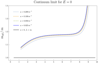
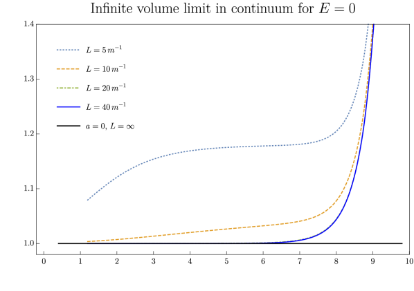
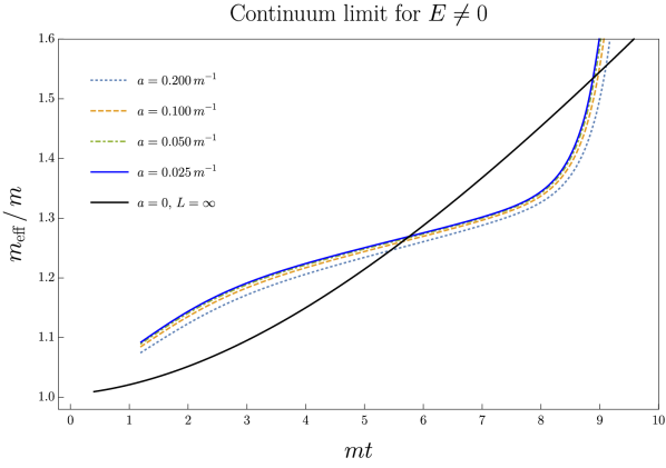
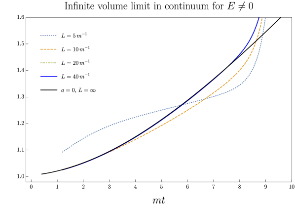
Figure 1: Comparison of effective mass function extracted from the effective correlator and the infinite-volume one in Eq. (9). For plots on the left we study the continuum limit: we make the lattice spacing finer and finer at fixed box size until convergence. For plots on the right, we focus on the finite volume effects. For the lower plots we use a value of the electric field of $a^{2}q{\cal E}=0.005$. For all plots the effective correlator is computed using Dirichlet boundary conditions in both directions. The lattice size in the time direction is $L_{t}=10m^{-1}$ and the source for the propagator is at $t_{0}=m^{-1}$.

II.3 Boundary conditions

In a finite volume the background field method requires careful handling of the external field at the boundaries. Even though the electric field is constant, the electrostatic potential $A_{\mu}$ has discontinuities at the edges of the box. For real electric fields, these discontinuities cannot be avoided. One workaround is to use imaginary fields with quantized values such that the ratio $q{\cal E}/(2\pi L_{x}L_{t})$ is an integer. This ensures uniform electric flux through all the $xt$ plaquettes and while the electrostatic potential is still discontinuous. One problem with this approach is that there is no obvious analytical continuation that connects this setup to a situation involving physical electric fields, so it is unclear whether the results computed in this setup are directly relevant for polarizability. Another problem is that in this setup different equivalent gauge choices for the external fields lead to results that are not connected by a gauge transformation. For example, in a gauge similar to the one used in Ref. Detmold:2010ts , of the form corresponding to Eq. (3), the Polyakov loops in the spatial directions depend on the choice of $t_{0}$ and, since the Polyakov loops are invariant under gauge transformations, different $t_{0}$ choices could lead to different results. This might not be a problem if the two gauges produce the same results, but it has to be verified, a posteriori. We choose to work with Dirichlet boundary conditions in both $x$ and $t$ directions. In this setup gauge invariance in the external field is guaranteed as we will discuss later. We can use either real or imaginary electric fields, and non-quantized values for the field strength, as small as needed for the quadratic terms due to polarizability to dominate.

On the other hand, using Dirichlet boundaries introduces a number of issues that must be dealt with. First issue is that the lowest energy state corresponds to a moving hadron. This is the main reason for the discrepancy present in the upper-right panel of Fig. 7 between the effective mass extracted from the finite-volume correlator and the infinite-volume one. For neutral hadrons, when extracting the energy from exponential decay of the correlators, we need an estimate of the hadron momentum to correct for the effect on the mass shift Lujan:2016ffj . When fitting the lattice QCD correlator to the one from the effective model, this ajustment is done automatically and the value extracted is directly the rest mass of the particle.

Another important effect is due to the pion interactions with the Dirichlet walls. Since hadrons are extended objects, they interact with the walls differently than the point-like particles described by the effective model. Away from the walls the hadrons move freely and the center-of-mass wavefunction corresponds to a free particle wave, but this does not hold true near the walls. The net effect is that the free wavefunction for the hadrons away from the walls has nodes that are not exactly aligned with the walls. To account for this difference we use a different distance between the walls in the effective model. The difference is related to the reflection scattering length introduced to capture the effect of this interaction for extended objects Lee:2010km ; Pine:2012zv . This effect will be studied using the pion correlator in the absence of an external field.

III Technical details and results

To fit the effective model we need to construct the hadron wavefunction profile between the Dirichlet walls. This requires us to calculate lattice QCD correlators as a function of both $x$ and $t$, the directions where we use Dirichlet boundary conditions. In the $y$ and $z$ directions we use periodic boundary conditions and we project the correlator to zero momentum in these directions,

$$G(x,t;A_{\mu},L)=\sum_{y,z}\langle 0|\hat{O}(x,y,z,t)\hat{O}^{\dagger}(x_{s},y_{s},z_{s},t_{s})|0\rangle,$$ (11)

where $\hat{O}=\bar{d}\gamma_{5}u$ is the interpolator for $\pi^{+}$ in the two-point function, is $(x_{s},y_{s},z_{s},t_{s})$ is the source for the quark correlators. Note that due to isospin symmetry between the $u$ and $d$ quarks, $\pi^{+}$ and $\pi^{-}$ ($\hat{O}=\bar{u}\gamma_{5}d$) have identical polarizability.

For the effective model we use the propagator derived in Eq. (8)

$$G_{0}(x,t;A_{\mu},\tilde{L})=K_{(x,t);(x,t)_{s}}^{-1}\,.$$ (12)

Above we emphasized that the correlators are functions of the external field $A_{\mu}$ and the distance between the walls: $\tilde{L}$ for the effective correlator and $L$ for QCD calculation.

We have generated the correlators with the position of quark sources fixed at $x_{s}/a=N_{x}/2+1$ and $t_{s}/a=6$. We use a coordinate system where the Dirichlet walls are positioned at $x=0$ and $x=L$ in the lattice QCD box. The effective model is aligned such that the source is at the same position and the walls are at $x=(L-\tilde{L})/2$ and $x=(L+\tilde{L})/2$. In effect the setup keeps the source position the same and changes the distance to the $x$-direction walls by the same amount. For both QCD and the effective model the time boundaries are $t=0$, and $t/a=(N_{t}+1)$. For QCD correlator, we take advantage of translation invariance of the system in $y$ and $z$ directions, and use sources at 64 locations for each configuration to obtain more statistics. The sources are spaced regularly at 8 positions on a $y$-$z$ grid and we use 8 different time translations. Note that since the gauge fields are generated with (anti-)periodic boundary conditions in time, time-translation is a symmetry of the ensemble. We apply the Dirichlet boundary conditions in time after the translation. A similar symmetry exists also in the $x$-direction but we did not take advantage of it in this study.

To find the appropriate distance between the walls for the model, we fit the lattice correlator to the effective model using different sizes for the model. We fit the correlators away from the walls to insure that the difference in the interactions with the walls do not affect the fit. The fit ranges, in both $x$- and $t$-directions are reported in Table 1.

Ensemble	$N_{x}N_{y}N_{z}N_{t}$	$N_{\texttt{cfg}}$	$\tilde{L}/a$	$x_{i}-x_{f}$	$t_{i}-t_{f}$
EN1	$16\times 16^{2}\times 32$	450	14.00(13)	$07-10$	$15-24$
EN2	$24\times 24^{2}\times 48$	300	21.50(17)	$07-18$	$15-32$
EN3	$30\times 24^{2}\times 48$	300	26.50(18)	$07-24$	$15-32$
EN4	$48\times 24^{2}\times 48$	300	44.00(72)	$07-42$	$15-32$

Table 1: Dynamical QCD ensembles on elongated lattice used in our study. In all cases $a=0.1245\,\mathop{\hbox{fm}}$ and $m_{\pi}=315\,\mathop{\hbox{MeV}}$. The last three columns show the effective spatial size and fit ranges.

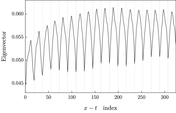
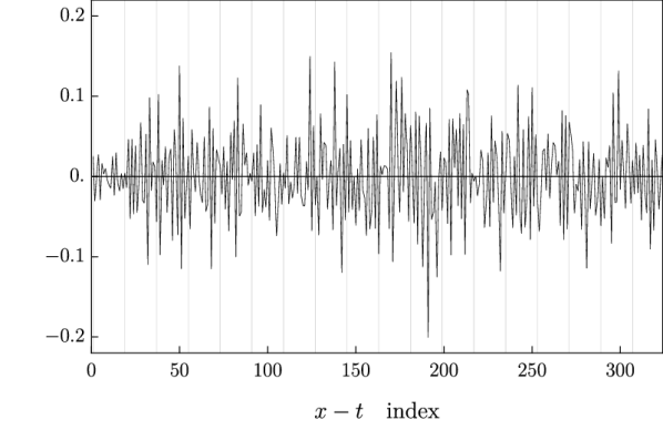
Figure 2: Eigenvectors corresponding to the largest (left) and smallest (right) eigenvalue of the covariance matrix, when including all points in the range listed in Table 1 for EN3. The thin vertical lines are the lines separating different time-slices; within each time slice, $x$ changes from left to right from $x_{i}$ to $x_{f}$.

III.1 Fitting procedure

To extract the mass from the lattice correlator we determine the mass in the effective model that minimizes the distance between the QCD correlator $G$ and the effective one $G_{0}$. The distance between the two correlators is defined via a $\chi^{2}$ function. The design of this distance function was guided by two main concerns: the fit procedure should produces the same results for all possible equivalent external field gauges and we want to accommodate the fact that the correlator is a complex valued function.

Assume that we perform on each configuration the measurements $y_{i}$ that are complex valued. The effective model value that is designed to match $y_{i}$ is assumed to be $f_{i}$. We define the $\chi^{2}$-function

$$\chi^{2}\equiv\delta^{\dagger}C^{-1}\delta\quad\text{with the {\em residues}}\quad\delta_{i}\equiv\left\langle y_{i}\right\rangle-f_{i}\,,$$ (13)

and the covariance matrix

$$C_{ij}\equiv\left\langle(y_{i}-\left\langle y_{i}\right\rangle)(y_{j}-\left\langle y_{j}\right\rangle)^{*}\right\rangle\,.$$ (14)

The covariance matrix is hermitian and the $\chi^{2}$-function is real and positive-definite. The minimization process will vary the parameters of the effective model to minimize $\chi^{2}$.

We are now interested in the action of the gauge transformations on the distance functions through the observables $y_{i}$. Assuming that the transformation acts linearly on the observables such that $y^{\prime}=Ty$ (that is $y^{\prime}_{i}=T_{ij}y_{j}$), with $T$ the same matrix for all configurations. Then $\left\langle y^{\prime}\right\rangle=T\left\langle y\right\rangle$ and if we have $f^{\prime}=Tf$, then $\delta^{\prime}=T\delta$. Similarly for the covariance matrix we have $C^{\prime}=TCT^{\dagger}$ and the distance function is then invariant, that is $(\chi^{2})^{\prime}=(\delta^{\prime})^{\dagger}(C^{\prime})^{-1}\delta^{\prime}=\chi^{2}$. This condition is satisfied if the observables $y_{i}$ are any subset of the point-to-point propagator function $G(x,t;A_{\mu},L)$ since under a gauge transformation, $(A,\phi)\to(A^{\prime},\phi^{\prime})$ with

$$\begin{split}A^{\prime}_{\mu}(x,t)&=A_{\mu}(x,t)+[\Lambda((x,t)+\hat{\mu})-\Lambda(x,t)]/a\\ \phi^{\prime}(x,t)&=e^{iq\Lambda(x,t)}\phi(x,t)\,,\end{split}$$ (15)

we have

$$G(x,t;A_{\mu}^{\prime},L)=e^{iq[\Lambda(x,t)-\Lambda(x_{s},t_{s})]}G(x,t;A_{\mu},L)\,.$$ (16)

Above we assumed that we use imaginary electric field. The same relation holds for the effective theory propagator $G_{0}$ so the distance between the point-to-point propagators is invariant under gauge transformations.

Given the discussion above it is then tempting to fit the lattice propagator at a subset of the $(x,t)$ positions, in the range included in Table 1. The problem is the presence of high frequency modes in the propagators close to the ultraviolet cutoff that are distorted due to lattice discretization. These modes can have an important contribution to the $\chi^{2}$-function. The smallest eigenvalues of the covariance matrix $C$ will have the biggest contribution to the $\chi^{2}$. This means that the lowest eigenvalues will drive the fitter and force the minimizer to a point in the parameter space that matches the distorted high frequency modes in the lattice QCD data instead of the physical long-range two-point function we are interested in. This is indeed the case for our calculation. In Fig. 2 we show the modes corresponding to the lowest and the highest eigenvalue in the covariance matrix, when we take the observables to be all space-time points in the range indicated in Table 1 for ensemble EN3. We see that the most important modes for the fitter, the ones that correspond to the lowest eigenvalue of the correlation matrix, are the ones that fluctuate rapidly along the spatial directions, the distorted high-frequency modes. To remedy this problem, we need to filter out the these high frequency modes from our observables.

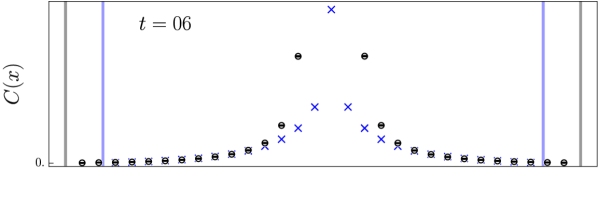
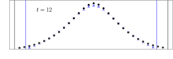
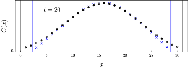
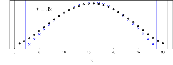
Figure 3: Spatial profile of the lattice correlator $G(x,t)$ (black) in zero electric field for EN3 is compared to the effective one (blue) at fixed time slices. The corresponding Dirichlet boundaries are represented by vertical lines.

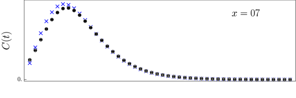
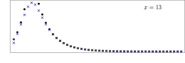
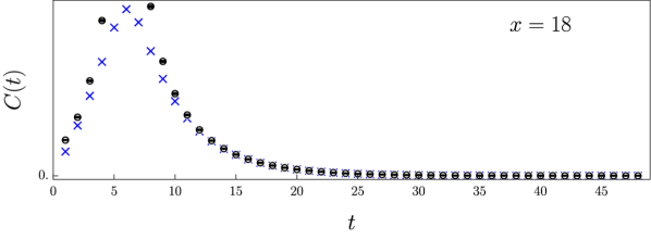
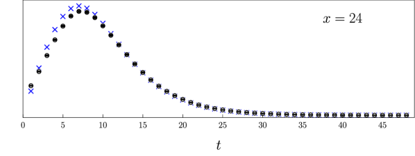
Figure 4: Similar to Fig 3, but for amplitude decay of the correlator at fixed $x$ locations.

For the zero-field propagators, we can just sum over the spatial position to filter out the high-frequency modes. This is akin to zero momentum projection used when fitting propagators with periodic boundary conditions. For our case this is only used to reduce the influence of the high-frequency modes, not to project to a particular momentum state. Our summation only extends over the interior points, away from the Dirichlet walls. However, this does not work for non-zero field propagators since gauge transformations act non-linearly on the observable defined via this summation. A different form is required to preserve gauge-invariance. In this work we use the following observables:

$$\begin{split}y(t)&=\sum_{x=x_{i}}^{x_{f}}L(x,t)G(x,t;A_{\mu}=0,L)\,\\ f(t)&={\cal A}\sum_{x=x_{i}}^{x_{f}}L(x,t)G_{0}(x,t;A_{\mu}=0,{\tilde{L}})\,.\end{split}$$ (17)

where

$$L(x,t)=\prod_{x^{\prime}=x_{i}}^{x-a}e^{-iqaA_{\mu}(x^{\prime},t)}\,,$$ (18)

and we fit for the amplitude ${\cal A}$ and mass $am$ that enters the definition of $G_{0}$. For the zero field case $L(x,t)=1$ and the summation produces the usual filtering. For the non-zero case, the gauge line $L(x,t)$ transforms as $L^{\prime}(x,t)=e^{iq[\Lambda(x_{i},t)-\Lambda(x,t)]}L(x,t)$. The observables then change under gauge transformation as

$$y^{\prime}(t)=e^{iqa[\Lambda(x_{i},t)-\Lambda(x_{s},t_{s})]}y(t)$$ (19)

and similarly for $f(t)$, and the distance function becomes gauge invariant.

The energy shift induced by the background field is very small, much smaller than the stochastic error on the extracted hadron masses. To extract the shift reliably we need to take into account the correlations between zero-field and non-zero field correlators. We perform simultaneous fits of the zero-field and non-zero field correlators. The residue vector $\delta=\{\delta_{0},\delta_{\cal E}\}$ includes the zero-field residue $\delta_{0}$ and the residue in the presence of the field $\delta_{\cal E}$ defined using the fit form

$$f(t)=({\cal A}+\Delta{\cal A})\sum_{x=x_{i}}^{x_{f}}L(x)G_{0}(x,t;A_{\mu},{\tilde{L}},am+\Delta am)\,.$$ (20)

The enlarged covariance matrix can be written as

$$C=\left(\begin{array}[]{cc}C_{00}&C_{0{\cal E}}\\ C_{{\cal E}0}&C_{{\cal E}{\cal E}}\end{array}\right).$$ (21)

The enlarged $\chi^{2}$ remains gauge invariant. Above we made explicit the dependence on the mass parameter. The fit parameters are ${\cal A}$, $am$, $\Delta{\cal A}$, and $\Delta am$. The mass shift $\Delta am$ is used to compute the polarizability.

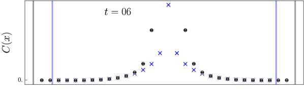
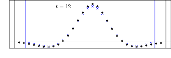
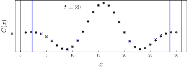
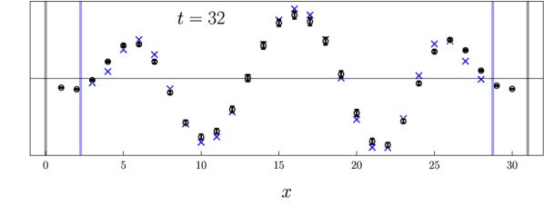
Figure 5: Real part of the lattice correlator $G(x,t)$ (black) in the presence of the electric field for EN3 is compared to the effective one (blue) at fixed time slices. The corresponding Dirichlet boundaries are represented by vertical lines.

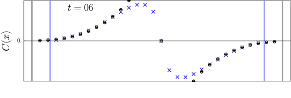
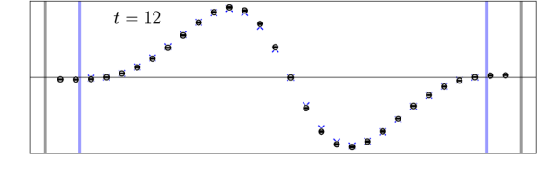
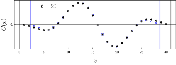
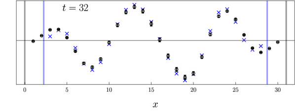
Figure 6: Similar to Fig 5, but for the imaginary part.

III.2 Effective range

As discussed earlier, the effective size $\tilde{L}$, the distance between the Dirichlet walls in the effective model, is slightly different from the distance between the walls in the QCD ensemble due to the interaction between the hadrons and the walls. To determine $\tilde{L}$ we use zero-field lattice QCD correlators. The ensembles used in this study are summarized in Table 1. For details about the generation of the ensembles see Niyazi:2020erg .

For each ensemble, we have done multiple fits to map out the dependence of the extracted mass on $\tilde{L}$. We choose the $x$ and $t$ ranges as wide as possible while maintaining a reasonable $\chi^{2}$, and look for an effective size $\tilde{L}$ that reproduces the mass obtained from periodic boundary conditions on the same ensembles Culver:2019qtx . For the three larger ensembles the finite-volume corrections for the pion mass are small and we used $am_{\pi}=0.1936(2)$. For the smallest ensemble, EN1, we used $am_{\pi}=0.1986(22)$ Lujan:2016ffj . The error-bars on $\tilde{L}$ were determined by jackknife. The dependence of the extracted mass on $\tilde{L}$ for our ensembles is shown in Fig. 7. We will discuss later the sensitivity of the mass-shift extraction on the effective size. The $\tilde{L}$ values determined from our ensembles and the fit ranges used are added to Table 1 and will be used in all of our subsequent fits. Note that the $\tilde{L}$ values were rounded up to the nearest half lattice-spacing to make the effective model calculations easier.

To see how well the effective model describes the lattice QCD correlators, we show in Fig. 3 some snapshots of the spatial profile (wavefunction) in the absence of electric field. Indeed, the Dirichlet walls force a standing wave in the $x$ direction. For the effective model there are no excited states in contrast to QCD where other excitations are present. However, in the pion channel the excited states lie much higher and the ground state pion becomes dominant as we move away from the source. We can see from the figure that this is indeed the case: the two correlators match very well as time progresses. This suggests that our effective models correctly captures the relevant dynamics. We note here that the correlators match well only after we adjust the effective distance $\tilde{L}$ appropriatedly. The same match is observed in the time decay of the correlation at fixed $x$ locations, as shown in Fig. 4.

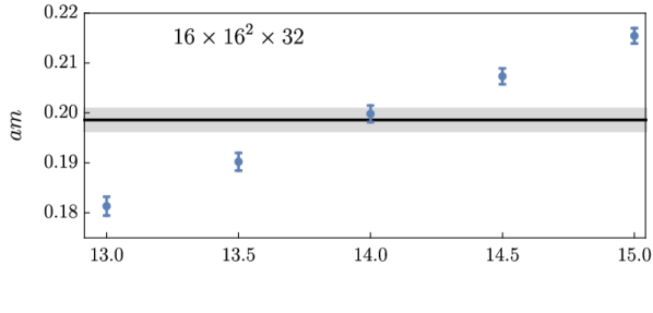
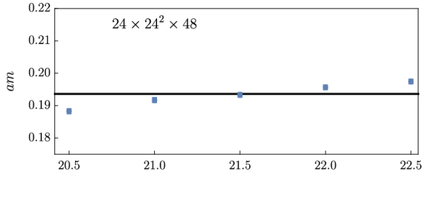
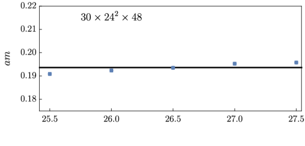
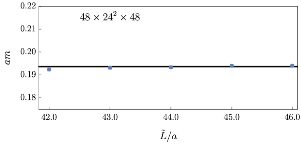
Figure 7: Dependence of $am$ on the distance between the Dirichlet walls for zero-field case. This is used to determine the effective lattice size $\tilde{L}$ in Table 1.

In the presence of the background electric field the correlators become complex. We show in Fig. 5 and Fig. 6 the real and imaginary parts separately of the charged particle correlator. For the effective correlator we use the same parameters, $am$ and $\cal A$, as in the zero-field case above. The agreement is very good since the corrections, $\Delta am$ and $\Delta{\cal A}$, associated with the external field ($a^{2}q_{d}{\cal E}=10^{-2}$ in this case) are minute. Interestingly, the wavefunction develops nodes between the walls in the presence of background electric field. It is tempting to think that this is due to the acceleration in the presence of the field, but in fact this is due to the gauge choice for the external field.

III.3 Polarizability extraction

To determine the pion polarizbility, we computed the lattice QCD correlators $G(x,t)$ on the four ensembles in Table 1 for charged pions, and carried out correlated fits as described above. We have used the same fit region that we had used when determining $\tilde{L}$ of the effective model in Table 1. Furthermore, for ensembles EN2, EN3, and EN4 which have the same temporal extension, we have fixed the temporal fit range to be the same for all of them.

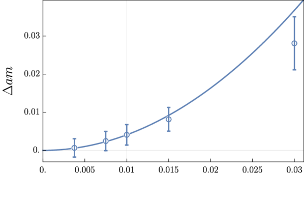
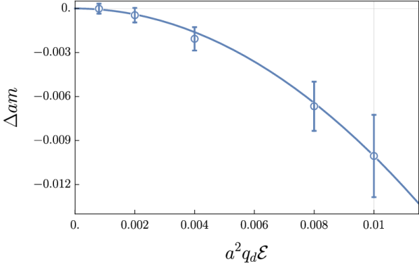
Figure 8: Mass shift as a function of the electric field for EN1 (top) and EN4 (bottom). The curves plotted here are the quadratic function which goes through zero and the central value of $\Delta am$ at $a^{2}q_{d}\mathcal{E}=0.01$. The quadratic behavior breaks down for larger values of the electric field since the higher-order corrections to the energy of the pion dominate.

Ensemble	$\Delta am$	$\alpha_{\pi^{\pm}}\,[10^{-4}\mathop{\hbox{fm}}^{3}]$	$\chi^{2}/{\rm dof}$
EN1	0.0041(27)	$1.30(84)$	1.4
EN2	0.0013(14)	$0.41(43)$	1.6
EN3	0.0040(16)	$1.26(50)$	1.4
EN4	-0.0101(28)	$-3.17(87)$	1.6

Table 2: Mass shift in lattice units and extracted electric polarizability for charged pions for a pion mass of $315\mathop{\hbox{MeV}}$.

To make sure that we are extracting the quadratic response to the electric field, we compute the mass shift for a sequence of increasing values for the electric field strength. In Fig. 8 we plot the mass shift as a function of field strength for the smallest ensemble (EN1) and the largest (EN4). We see that the value of the electric field used in this study is indeed in the regime where the mass shift scales quadratically with the electric field strength. For our study we used the smallest value of the electric field where the mass-shift is not statistically compatible with zero on the smallest ensemble (EN1): $a^{2}q_{d}{\cal E}=0.01$.

The fit results are summarized in Table 2. The mass shifts are indeed small when compared to the particle mass. The conversion from lattice units to physical units from Eq. 1 is given by

$$\alpha_{\pi^{\pm}}=\frac{2}{a{\cal E}^{2}}\delta am$$ (22)

where $a=0.1245$ fm, $e^{2}=1/137$, and $a^{2}q_{d}{\cal E}=0.01$.

The dominant sources of systematic errors are the choice of the fit range in the spatial and temporal direction, and the value of $\tilde{L}$ using in the effective model. To determine their contribution we analyze the sensitivity of the polarizability to expected changes in these parameters. For the fitting range, we reduced both the $x$ and $t$-ranges by one unit of lattice spacing. For $\tilde{L}$ we vary it within the error bands reported in Table 1. The results are included in Table 3. We note here that for the three largest ensembles used in our study the finite-volume corrections estimate from ChPT is less than 10% Tiburzi:2008pa .

Ensemble		Original		$x_{i}+1$ $x_{f}-1$	$t_{i}+1$	$\tilde{L}-\delta\tilde{L}$
EN1		1.30(84)		1.22(85)	1.18(87)	1.57(85)
EN2		0.41(43)		0.35(43)	0.51(47)	0.68(43)
EN3		1.26(50)		1.26(50)	1.34(54)	1.50(50)
EN4		-3.17(87)		-3.13(85)	-4.4(1.2)	-3.00(87)

Table 3: Sensitivity of the results on the choice of fit ranges and the model size. We compare the polarizability $\alpha_{\pi^{\pm}}$ extracted using our choice for the fit ranges with the value extracted for slightly different choices. In this table $\delta{\tilde{L}}$ is the error on $\tilde{L}$ reported in Table 1.

In Fig. 9 we plot the results for polarizability as a function of the lattice extent in the field direction. Our results are compared with the ChPT value of Holstein:2013kia

$$\alpha_{\pi^{\pm}}=\frac{\alpha_{\text{em}}}{8\pi^{2}m_{\pi}f_{\pi}^{2}}\frac{h_{A}}{h_{V}}=0.93(6)\times 10^{-4}\,{\mathop{\hbox{fm}}}^{3},$$ (23)

evaluated at our pion mass of $m_{\pi}=315\mathop{\hbox{MeV}}$. To compute the pion decay constant for our pion mass we used NLO ChPT expression with low-energy constant $\overline{\ell}_{4}$ from the FLAG review Aoki:2019cca to get $f_{\pi}=106\mathop{\hbox{MeV}}$. For the form factors ratio $h_{A}/h_{V}$ we used the experimental value $0.469\pm 0.031$ Holstein:2013kia which also gives the dominant source of error to the ChPT estimate. For the smallest ensembles, our results are in agreement with the ChPT estimate. For the largest volume (EN4) the polarizability turns, surprisingly, negative. We do not have an explanation for this behavior but we note that there are other lattice calculations of pion polarizability for comparable quark masses that are at variance with ChPT expectations. One is on magnetic polarizability that is expected to satisfy $\beta_{\pi^{+}}=-\alpha_{\pi^{+}}$, a calculation for $m_{\pi}=296\mathop{\hbox{MeV}}$ finds $\beta_{\pi^{+}}=0.35(11)\times 10^{-4}\mathop{\hbox{fm}}^{3}$. Another calculation of the “connected” neutral pion electric polarizability—where the disconnected diagrams are not included—finds that the polarizability turns negative for $m_{\pi}<350\mathop{\hbox{MeV}}$ Lujan:2014kia ; Lujan:2016ffj although the ChPT expectations are that this value should be positive Detmold:2009dx .

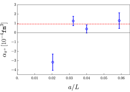
Figure 9: Volume dependence of the extract polarizability at pion mass of $m_{\pi}=315\mathop{\hbox{MeV}}$. The dotted line is prediction from leading-order ChPT.

IV Conclusion

Computing electric polarizability for charged hadrons has been a challenge for lattice QCD due to the acceleration experienced by charged particles in the background electric field. Using the lightest charged hadron, the pion, as an example, we presented a method to extract the electric polarizability. The method relies on an effective field model that is designed to capture the behavior of the charged pion in a box with the same geometry as that used in lattice simulations. This has proven crucial since the infinite-volume version of the model fails to account for the significant finite-volume effects. This is important to isolate the energy shift due only to the deformation of the hadron from the effects due to its motion in the electric field.

To fit the lattice QCD correlators we need to compute its $x$ and $t$ dependence separately to match the effective model. We construct a $\chi^{2}$-function that utilizes information in both the real and imaginary parts of the correlator simultaneously and is invariant under gauge transformations of the background field.

Since we use Dirichlet boundary conditions, we are not limited to just quantized values under periodic boundary conditions. We can dial the electric field continuously and choose values that give better signals.

We extract the pion polarizability on a set of ensembles with different distance between the Dirichlet walls. For the pion mass $m_{\pi}=315\mathop{\hbox{MeV}}$ used in this study, the results on the smallest three ensembles are compatible with a small positive value for $\alpha$, a value in agreement with ChPT predictions. However, on the largest ensemble the polarizability is negative, a puzzling result. We have checked the sensitivity of the polarizability on the fitting range and the effective distance between the walls employed in the effective model. The effect of varying these parameters is smaller than the stochastic error and cannot explain the shift to negative values for the polarizability. We note that there are other lattice calculations of electromagnetic polarizabilities at similar pion mass that in tension with ChPT predictions.

In this paper we focused more on the technical aspects of the extraction method. Looking to the future, in order to compare with experiments, we need to extrapolate to physical quark masses. We expect that as we approach the physical mass ChPT predictions become more reliable and should offer a strong check for our results. In particular we plan to investigate the puzzling result we got on the largest volume in this study. ChPT predicts a $1/m_{\pi}$ rise as the pion mass is lowered (see Eq. 23) so the signal might be stronger at smaller pion masses. Another direction we plan to investigate is the effect of lattice discretization. As an additional check of the fitting procedure, we plan to apply the same method to neutral mesons on the same set of ensembles where simple exponential fits were previously employed Lujan:2016ffj ; Lujan:2014kia . Another systematic effect, namely charging the sea quarks, is not addressed here, though such effects are expected to be small Freeman:2014kka ; Freeman:2013eta . In the long run, an extension to baryons would be desirable with an eye towards the proton electric polarizability which is more precisely measured than charged pions but is less well studied on the lattice.

- (1) A.I. L’vov, Theoretical aspects of the polarizability of the nucleon, Int. J. Mod. Phys. A 8 (1993) 5267.
- (2) M. Moinester and S. Scherer, Compton Scattering off Pions and Electromagnetic Polarizabilities, Int. J. Mod. Phys. A 34 (2019) 1930008 [1905.05640].
- (3) V. Lensky and V. Pascalutsa, Predictive powers of chiral perturbation theory in Compton scattering off protons, Eur. Phys. J. C 65 (2010) 195 [0907.0451].
- (4) F. Hagelstein, Nucleon Polarizabilities and Compton Scattering as a Playground for Chiral Perturbation Theory, Symmetry 12 (2020) 1407 [2006.16124].
- (5) H.W. Griesshammer, J.A. McGovern, D.R. Phillips and G. Feldman, Using effective field theory to analyse low-energy Compton scattering data from protons and light nuclei, Prog. Part. Nucl. Phys. 67 (2012) 841 [1203.6834].
- (6) H.R. Fiebig, W. Wilcox and R.M. Woloshyn, A Study of Hadron Electric Polarizability in Quenched Lattice QCD, Nucl. Phys. B 324 (1989) 47.
- (7) M. Lujan, A. Alexandru, W. Freeman and F.X. Lee, Finite volume effects on the electric polarizability of neutral hadrons in lattice QCD, Phys. Rev. D94 (2016) 074506 [1606.07928].
- (8) M. Lujan, A. Alexandru, W. Freeman and F. Lee, Electric polarizability of neutral hadrons from dynamical lattice QCD ensembles, Phys. Rev. D89 (2014) 074506 [1402.3025].
- (9) W. Freeman, A. Alexandru, M. Lujan and F.X. Lee, Sea quark contributions to the electric polarizability of hadrons, Phys. Rev. D 90 (2014) 054507 [1407.2687].
- (10) W. Freeman, A. Alexandru, F.X. Lee and M. Lujan, Update on the Sea Contributions to Hadron Electric Polarizabilities through Reweighting, in 31st International Symposium on Lattice Field Theory, 10, 2013 [1310.4426].
- (11) B.C. Tiburzi, Hadrons in Strong Electric and Magnetic Fields, Nucl. Phys. A814 (2008) 74 [0808.3965].
- (12) W. Detmold, B.C. Tiburzi and A. Walker-Loud, Lattice QCD in Background Fields, 0908.3626.
- (13) A. Alexandru and F.X. Lee, The Background field method on the lattice, PoS LATTICE2008 (2008) 145 [0810.2833].
- (14) F.X. Lee, L. Zhou, W. Wilcox and J.C. Christensen, Magnetic polarizability of hadrons from lattice QCD in the background field method, Phys. Rev. D 73 (2006) 034503 [hep-lat/0509065].
- (15) F.X. Lee, R. Kelly, L. Zhou and W. Wilcox, Baryon magnetic moments in the background field method, Phys. Lett. B 627 (2005) 71 [hep-lat/0509067].
- (16) M. Engelhardt, Neutron electric polarizability from unquenched lattice QCD using the background field approach, Phys. Rev. D 76 (2007) 114502 [0706.3919].
- (17) R. Bignell, W. Kamleh and D. Leinweber, Magnetic polarizability of the nucleon using a Laplacian mode projection, Phys. Rev. D 101 (2020) 094502 [2002.07915].
- (18) A. Deshmukh and B.C. Tiburzi, Octet Baryons in Large Magnetic Fields, Phys. Rev. D 97 (2018) 014006 [1709.04997].
- (19) G.S. Bali, B.B. Brandt, G. Endrődi and B. Gläßle, Meson masses in electromagnetic fields with Wilson fermions, Phys. Rev. D 97 (2018) 034505 [1707.05600].
- (20) F. Bruckmann, G. Endrodi, M. Giordano, S.D. Katz, T.G. Kovacs, F. Pittler et al., Landau levels in QCD, Phys. Rev. D 96 (2017) 074506 [1705.10210].
- (21) A. Parreno, M.J. Savage, B.C. Tiburzi, J. Wilhelm, E. Chang, W. Detmold et al., Octet baryon magnetic moments from lattice QCD: Approaching experiment from a three-flavor symmetric point, Phys. Rev. D 95 (2017) 114513 [1609.03985].
- (22) E.V. Luschevskaya, O.E. Solovjeva and O.V. Teryaev, Magnetic polarizability of pion, Phys. Lett. B 761 (2016) 393 [1511.09316].
- (23) NPLQCD collaboration, Magnetic structure of light nuclei from lattice QCD, Phys. Rev. D 92 (2015) 114502 [1506.05518].
- (24) W. Detmold, B.C. Tiburzi and A. Walker-Loud, Extracting Nucleon Magnetic Moments and Electric Polarizabilities from Lattice QCD in Background Electric Fields, Phys. Rev. D81 (2010) 054502 [1001.1131].
- (25) W. Andersen and W. Wilcox, Lattice charge overlap. 1. Elastic limit of pi and rho mesons, Annals Phys. 255 (1997) 34 [hep-lat/9502015].
- (26) W. Wilcox, Lattice charge overlap. 2: Aspects of charged pion polarizability, Annals Phys. 255 (1997) 60 [hep-lat/9606019].
- (27) Z. Davoudi and W. Detmold, Implementation of general background electromagnetic fields on a periodic hypercubic lattice, Phys. Rev. D 92 (2015) 074506 [1507.01908].
- (28) M. Engelhardt, Exploration of the electric spin polarizability of the neutron in lattice QCD, PoS LATTICE2011 (2011) 153 [1111.3686].
- (29) F.X. Lee and A. Alexandru, Spin Polarizabilities on the Lattice, PoS LATTICE2011 (2011) 317 [1111.4425].
- (30) W. Detmold, B.C. Tiburzi and A. Walker-Loud, Electromagnetic and spin polarisabilities in lattice QCD, Phys. Rev. D73 (2006) 114505 [hep-lat/0603026].
- (31) E. Shintani, S. Aoki, N. Ishizuka, K. Kanaya, Y. Kikukawa, Y. Kuramashi et al., Neutron electric dipole moment with external electric field method in lattice QCD, Phys. Rev. D 75 (2007) 034507 [hep-lat/0611032].
- (32) W. Detmold, B.C. Tiburzi and A. Walker-Loud, Extracting Electric Polarizabilities from Lattice QCD, Phys. Rev. D 79 (2009) 094505 [0904.1586].
- (33) A. Alexandru, M. Lujan, W. Freeman and F. Lee, Pion electric polarizability from lattice QCD, AIP Conf. Proc. 1701 (2016) 040002 [1501.06516].
- (34) H.J. Rothe, Lattice gauge theories: An Introduction, World Sci. Lect. Notes Phys. 43 (1992) 1.
- (35) J.S. Schwinger, On gauge invariance and vacuum polarization, Phys. Rev. 82 (1951) 664.
- (36) D. Lee and M. Pine, How quantum bound states bounce and the structure it reveals, Eur. Phys. J. A 47 (2011) 41 [1008.5187].
- (37) M. Pine and D. Lee, Effective Field Theory for Bound State Reflection, Annals Phys. 331 (2013) 24 [1206.6280].
- (38) H. Niyazi, A. Alexandru, F.X. Lee and R. Brett, Setting the scale for nHYP fermions with the Lüscher-Weisz gauge action, Phys. Rev. D 102 (2020) 094506 [2008.13022].
- (39) C. Culver, M. Mai, A. Alexandru, M. Döring and F.X. Lee, Pion scattering in the isospin channel from elongated lattices, Phys. Rev. D 100 (2019) 034509 [1905.10202].
- (40) B.C. Tiburzi, Volume Effects for Pion Two-Point Functions in Constant Electric and Magnetic Fields, Phys. Lett. B 674 (2009) 336 [0809.1886].
- (41) B.R. Holstein and S. Scherer, Hadron Polarizabilities, Ann. Rev. Nucl. Part. Sci. 64 (2014) 51 [1401.0140].
- (42) Flavour Lattice Averaging Group collaboration, FLAG Review 2019: Flavour Lattice Averaging Group (FLAG), Eur. Phys. J. C 80 (2020) 113 [1902.08191].