Efficient Parallel Self-Adjusting Computation

Abstract

Self-adjusting computation is an approach for automatically producing dynamic algorithms from static ones. The approach works by tracking control and data dependencies, and propagating changes through the dependencies when making an update. Extensively studied in the sequential setting, some results on parallel self-adjusting computation exist, but are either only applicable to limited classes of computations, such as map-reduce, or are ad-hoc systems with no theoretical analysis of their performance.

In this paper, we present the first system for parallel self-adjusting computation that applies to a wide class of nested parallel algorithms and provides theoretical bounds on the work and span of the resulting dynamic algorithms. As with bounds in the sequential setting, our bounds relate a “distance” measure between computations on different inputs to the cost of propagating an update. However, here we also consider parallelism in the propagation cost.

The main innovation in the paper is in using Series-Parallel trees (SP trees) to track sequential and parallel control dependencies to allow propagation of changes to be applied safely in parallel. We show both theoretically and through experiments that our system allows algorithms to produce updated results over large datasets significantly faster than from-scratch execution. We demonstrate our system with several example applications, including algorithms for dynamic sequences and dynamic trees. In all cases studied, we show that parallel self-adjusting computation can provide a significant benefit in both work savings and parallel time.

1 Introduction

Self-adjusting computation is an approach to automatically, or semi automatically, convert a (suitable) static algorithm to a dynamic one [20, 27, 4, 5, 6, 1, 26, 19]. Most often, self-adjusting computation is implemented in the form of a change propagation algorithm. The idea, roughly, is to run a static algorithm while keeping track of data dependencies. Then when an input changes (e.g. adding an edge to a graph), the change can be propagated through the computation, updating intermediate values, creating new dependencies, and updating the final output. Not all algorithms are suitable for the approach—for some, updating a single input value could propagate changes through most of the computation. To account for how much computation needs to be rerun, researchers have studied the notion of “stability” [6, 1] over classes of changes. The goal is to bound the “distance” between executions of a program on different inputs based on the distance between the inputs. For example, for an appropriate sorting algorithm adding an element to the unsorted input list ideally would cause at most $O(\log n)$ recomputation, and that recomputation could be propagated with a constant factor overhead. This would lead to the performance of a dynamic binary search tree.

In the sequential setting this approach has been applied to a wide variety of algorithms, with various bounds on the stability, and also cost of change propagation as a function of the computational distance. Applications includes dynamic trees [6], kinetic data structures [9, 8, 10], convex hulls [3], Huffman coding [7], and Bayesian inference [11].

More recent work [2, 13, 18, 25, 12] has studied applying change propagation in parallel, allowing for batch dynamic updates—e.g., adding a set of edges to an existing graph and then propagating those changes in parallel. Batch updates are particularly important in practice due to the rapid rate of modifications to very large data sets such as the web graph or social networks. Furthermore, in principle, parallelism and change propagation should work well together since algorithms with shallow dependence chains tend both to be good for parallelism (since fewer dependencies means more task can run in parallel) and for dynamic updates (since changes will not have to propagate as deeply). Indeed several researchers have studied the approach and developed systems in the applied setting, which show good performance improvements [13, 18, 12] on tasks such as map-reduce.

In the theoretical setting, recent work has studied bounds on the cost of change propagation for a class of so-called “round-synchronous” computations [2]. This was applied to generate efficient algorithms for batch-dynamic trees, supporting batches of links and cuts among other operations. However, the round-synchronous nature limits the applicability to certain algorithms that fit the restrictive model.

In this paper we develop a more general framework for supporting self-adjusting computation for arbitrary nested-parallel algorithms. We prove bounds on the cost of change propagation in the framework based on an appropriately defined distance metric. We have also implemented the framework and run experiments on a variety of benchmarks. A nested parallel program is one that is built from arbitrary sequential and parallel composition. A computation is defined recursively as either two computations that are composed in parallel (a fork), two that are composed sequentially, or the base case which is a sequential strand. Multiway forking can easily be implemented by nesting parallel compositions.

The crux of our technique is to represent a computation by a dependency graph that is anchored on a Series-Parallel tree [23], or SP tree for short. An SP tree corresponds to the sequential and parallel composition of binary nested parallel programs—i.e., parallel composition consists of a $P$ node with two children (the left-right order does not matter), and sequential composition consists of an $S$ node with two children (here the order does matter). The leaves are sequential strands of computation, and can just be modeled as leaf $S$ nodes. The SP tree represents the control dependencies in the program—i.e., that a particular strand needs to executed before another strand. We additionally introduce R nodes to indicate data reads, which are used to track data dependencies between writes and reads—i.e., that a particular read depends on the value of a particular write. Together we refer to the trees as RSP trees, corresponding to the three types of nodes. The RSP tree of a computation allows propagating a change in a way that respects sequential control dependencies while allowing parallelism where there is no dependence. We prove that a parallel change propagation algorithm can propagate changes through the computation in a manner that is both efficient and scalable.

Programs written in our framework write their inputs and any non-local values that depend on them into “modifiable references”, or modifiables for short, which track all reads to them and facilitate change propagation. Like previous work on sequential change propagation [6], we achieve our efficiency by restricting input programs to those which write to each modifiable exactly once. All race-free functional programs satisfy this restriction. We note that since local variables do not need to be tracked, they are not bound by this restriction, so the scope of programs amenable to our framework is not just those which are purely functional.

Roughly speaking, given two executions of the same algorithm on different inputs, we define the computation distance to be the work that is performed by one but not the other (see Definition 4.2 for the full definition). We then show the following theorem that bounds the runtime of the change propagation algorithm as a function of computation distance.

Theorem 1.1 (Efficiency).

Consider an algorithm $A$, two input states $I$ and $I^{\prime}$, and their corresponding RSP trees $T$ and $T^{\prime}$. Let $W_{\Delta}=\delta(T,T^{\prime})$ denote the computation distance, $R_{\Delta}$ denote the number of affected reads, $s$ denote the span of $A$, and $h$ denote the maximum heights of $T$ and $T^{\prime}$. Then, change propagation on $T$ with the dynamic update $(I,I^{\prime})$ runs in $O(W_{\Delta}+R_{\Delta}\cdot h)$ work in expectation and $O(s\cdot h)$ span w.h.p.

We have implemented the proposed techniques in a library for C++, which we call PSAC++ (Parallel Self-Adjusting Computation in C++). The library allows writing parallel self-adjusting programs by using several small annotations in a style similar to writing conventional parallel programs. Self-adjusting programs can respond to changes to their data by updating their output via the built-in change propagation. Our experiments with several applications show that parallel change propagation can handle a broad variety of batch changes to input data efficiently and in a scalable fashion. For small changes, parallel change propagation can yield very significant savings in work; such savings can amount to orders of magnitude of improvement. For larger changes, parallel change propagation may save some work, and still exploit parallelism, yielding improvements due to both reduction in work and an increase in scalability. We summarize the contributions of the paper as follows:

• A general approach for parallel change propagation based on using RSP trees to safely propagate changes in the correct order while allowing parallelism in the propagation.

• Theoretical bounds on the work (sequential time) and span (parallel time) of our algorithms.

• An implementation as C++ library, with six example applications to study as benchmarks.

• Experimental results that confirm what is backed up by our theoretical analysis, that parallel change propagation is efficient for a range of applications.

1.1 Technical Overview

The idea of the change propagation algorithm is first to run an algorithm on some initial input while keeping a trace of reads and writes to “non local” locations. This trace can be thought of as a write-read dependence graph, indicating what reads depend on what writes (also called a data dependence graph). Along with each read the trace also stores the code that was run on the value, and maintains some form of control ordering of the execution. When an input is updated at particular locations, the change propagation algorithm knows what read those locations and reruns them. This can cause new reads and writes that both update the trace, and create changes that have to propagated to their readers. Importantly, and one of the biggest challenges in change propagation, is that the reads that rerun have to do so in control order, otherwise they could use stale information. For example, if a read A, and a later a read B in program control order both need to be rerun, running B first might miss updates by A. Since A could do something different when rerun, the trace might not even know there will be a data dependence between them (A is now going to write to something B reads). This means that the topological order on the trace’s data dependence graph in insufficient for safety, and that control dependencies also need to be considered.

In the sequential setting, the total order of all instructions is typically maintained using a dynamic list-maintenance data structure [21] keeping all reads in time order. The structure needs to be dynamic since during propagation new computation can be added, and old deleted, at arbitrary points in the ordering. During change-propagation, all reads that are affected by a write are placed in a priority queue prioritized by this order, and always processing the earliest first.

For our work on parallel change propagation, the broad idea is to organize the control dependencies of the program around the RSP tree. Unlike the sequential case, instead of having a total order of execution time, the RSP tree effectively keeps track of the parallel partial order of control dependencies among the strands. As with the sequential case, we also keep track of all write-read data dependencies. Unlike the sequential algorithm which uses a priority queue of time order, our algorithm instead uses the RSP tree itself to maintain the partial order among strands—and this allows running multiple tasks in parallel during the propagation.

The initial run builds the RSP tree. It stores on each read (R) node a closure to rerun if the value it read changes. When the input is modified, the change-propagation algorithm identifies all readers of the changed values. We refer to these as the affected readers. Now, instead of adding them to a priority queue by sequential time order, the algorithm makes some markings in the RSP tree. In particular it starts at each affected reader and marks all ancestors in the RSP tree. It then traverses the RSP tree and using the marks finds readers that require and are safe to rerun, i.e., only descending if a node is marked. Whenever it gets to a $P$ node, the algorithm traverses down whichever children are marked (either left, right, or both in parallel), and whenever it gets to an internal $S$ node, it traverses down the left branch if it is marked, and then the right branch if it is marked. At an $S$ node the algorithm never goes down both branches simultaneously since that would be unsafe—it would run strands in parallel that should be run sequentially.

Whenever the traversal meets an affected reader, change propagation runs the closure associated with the reader and updates the resulting computation and its corresponding subtree of the RSP tree, possibly cascading new reads and writes and marking additional regions of the RSP tree for additional propagation. Once the marked regions of the tree have all been traversed, change propagation is complete and the computation will be fully up to date.

1.2 Related Work

While there is little work on fully fledged parallel self-adjusting computation, a few systems have been developed.

Incoop. On the programming language side, Bhatodia et al. [13] develop a framework for self-adjusting computation in the map-reduce paradigm. Their system specifically targets map-reduce-style computations in a distributed model of computation, and does not provide any theoretical guarantees on the runtime of updates.

Two for the price of one. Burckhartd et al. [18] were the first to develop a general-purpose system for parallel self-adjusting computation. They do so by extending the so-called concurrent revisions model with primitives for self-adjusting computation. This model enables programs to express fork-join parallelism with versioned types that allow multiple threads to concurrently write to an object that is automatically aggregated at the join point, in a style similar to Cilk reducers [24]. Their algorithm for self-adjusting computation then essentially performs memoisation of the versioned writes done by each fork, allowing them to be looked up and re-used if their dependencies haven’t changed. Their work is evaluated on a set of five benchmark problems, where it is demonstrated experimentally that the combination of parallelism and self-adjusting computation is worthwhile, producing both work savings and parallel time speedups. This work, however, is purely experiential and does not provide theoretical guarantees on the runtime of updates.

iThreads. Bhatodia et al. [12] develop iThreads, a pthreads drop-in replacement that automatically dynamizes the underlying program. The advantage of such a system is that dynamization is completely automatic; the programmer does not even have to annotate their code or add additional primitives to perform self-adjusting computation. The corresponding downside is that the dynamization is very coarse grained, since the only units of work that can be re-executed are the entire pthread computations. The user is therefore unable to fine tune the dynamism, which is often important to optimize self-adjusting programs. Theoretical guarantees on the runtime of updates are not provided.

PAL. Hammer et al. [25] present Parallel Adaptive Language (PAL), a proposed (though not fully implemented) language for parallel self-adjusting computation. Like other works, including ours, it represents the trace of a computation using a tree structure, which encodes parallel and sequential dependencies between computations and the data that they read. Their proposed algorithm, however, requires several nontrivial data structures, some of which, such as an efficient concurrent fully dynamic lowest common ancestor (LCA) structure, do not yet exist. Their evaluation therefore consists of a simulation of the work that would be performed by the algorithm if said data structures were available, rather than a realistic evaluation.

1.3 Model of Computation

We analyze algorithms in the work-span model, where work is the total number of instructions performed by the algorithm and span (also called depth) is the length of the longest chain of sequentially dependent instructions [14]. The model can work-efficiently cross simulate the classic CRCW PRAM model [14], and the more recent Binary Forking model [16], incurring at most an additional $O(\log^{*}(n))$ factor overhead in the depth due to load balancing. An algorithm with work $W$ and span $s$ can be ran on a $p$-processor PRAM in $O(W/p+s)$ time [17].

2 Framework

Our framework for parallel self-adjusting computation is built around a set of core primitives that are easy to integrate into existing algorithms. In this section, we describe these primitives and give an example algorithm for illustration.

write(dest: $\alpha\ \textbf{mod}{}$, value : $\alpha$)
alloc_mod(T: type) : T mod
read(m : $(\alpha_{1}\ \textbf{mod},...,\alpha_{k}\ \textbf{mod})$, r : $\alpha_{1}\times...\times\alpha_{k}\mapsto()$)
par(left_f : $()\mapsto()$ , right_f : $()\mapsto()$)
run($f:()\mapsto()$) : $S$
propagate(root : $S$)

Figure 1: Interface for Parallel Self-Adjusting Computation

Modifiables. The primary mechanism by which computations are dynamised is through the use of modifiable variables. A modifiable variable, or modifiable for short, is either a value that is part of the input to the algorithm, or a nonlocal variable whose value depends on the value of another modifiable variable. Algorithms are dynamised by placing their inputs in modifiables, and ensuring that all nonlocal variables whose values depend on a modifiable are also placed in modifiables. When a modifiable is updated, our framework can then automatically determine which values are affected by the resulting changes, and automatically propagate the appropriate updates.

Modifiables can be allocated either statically, i.e. before the computation is run, or dynamically, in which case their lifetime will be tied to the scope of the computation that allocated them. Writing to modifiables is achieved using the write operation. We require that each modifiable is written to at most once during each run of the computation, and that modifiables are not read before they are written. We also require that modifiables are only read from and written to by computations that are in the dynamic (nested) scope of the computation that allocated it.

Read operations. To ensure that dependencies are tracked, modifiables must be read using the read operation. read reads the values of the given modifiables and invoke the given reader function with their current values as arguments.

Parallelism. We support fork-join parallelism through a binary fork operation par, which takes two code thunks and executes them in parallel.

Control. Computations are initiated with the run operation, which returns a handle to the computation (represented by the root of the RSP tree). After making changes to the input, changes are propagated using the propagate operation.

Additional primitives. For convenience, we also support an alloc_array operation and a corresponding read_array operation for allocating and reading arrays of modifiables. We also support a parallel_for primitive, which executes a given function over a range of values in parallel. We omit the details of these primitives.

A note on randomness. We require that all algorithms implemented in our framework be deterministic. That is, given some input, if re-executed they must produce exactly the same output. It is still possible, and indeed we have several in our application examples, to implement randomized algorithms. To do so, the randomness must simply be pre-generated before executing the computation to ensure that, when re-executed, the same results will be obtained.

Example. To illustrate our framework, we give an implementation of a parallel divide-and-conquer sum function. See Algorithm 1. Note that in our pseudocode, for readability, we denote reads using the syntax:

with read(mods…) as args… do $f$(args…)

This computation is static in the sense that regardless of updates, the RSP tree will always look the same. In general, our system supports arbitrary changes, even if they lead to wildly different trees.

Algorithm 1 Parallel self-adjusting sum

1:function Sum(A[lo…hi] : int mod array, res : int mod)

2:   if lo = hi - 1 then

3:     with read(A[lo]) as x do

4:        write(res, x)      

5:   else

6:     local mid $\leftarrow$ lo + (hi - lo) / 2

7:     local left_res $\leftarrow$ alloc_mod(int)

8:     local right_res $\leftarrow$ alloc_mod(int)

9:      par(function $\Rightarrow$ Sum(A[lo…mid], left_res), function $\Rightarrow$ Sum(A[mid…hi], right_res))

10:     with read(left_res, right_res) as x, y do

11:        write(res, x + y)         

3 Change Propagation Algorithm

We use a variant of SP trees (see introduction) extended with read (R) nodes, which we call RSP trees. A read is tracked in the RSP tree by creating an R node as the left child of the current S node whenever a reader is executed. The reader code then executes in the subtree of the R node and the subsequent continuation proceeds in the sibling node. The full semantics for RSP trees for any given computation is defined by the algorithms in this section.

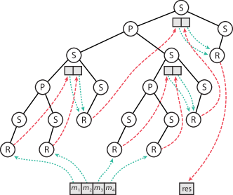
Figure 2: The RSP tree of the divide-and-conquer sum algorithm on an input of size four. Dynamically allocated modifiables are depicted underneath the $S$ node that allocated them. Writes and reads to/from modifiables are shown as red (long-dashed) and green (short-dashed) arrows respectively.

Figure 2 shows an example RSP tree for the divide-and-conquer sum computation of Algorithm 1 on an input of size four. We use green (short-dashed) arrows to show which read nodes read from which modifiables, and red (long-dashed nodes) to indicate which sequential computations wrote to which modifiables. The four $R$ nodes lowest in the tree correspond to the reads of the input, which occur at the base case of the algorithm. The $R$ nodes higher in the tree are the reads of the results of the recursive calls.

Our framework facilitates self-adjusting computation by first building the RSP tree during the initial run of the static algorithm. To execute dynamic updates, when a modifiable is written to, all of the read nodes that read from it, and all of their ancestors in the RSP tree are marked as pending re-execution. Change propagation then simply consists in traversing the RSP tree, ignoring paths which are not marked, since no changes are present, and re-executing the marked readers. Note that this re-execution destroys the old portion of the RSP tree corresponding to the read and generates a new one, meaning that the old and new computations can be entirely structurally different. Additionally, such re-execution may also write to subsequent modifiables that were also read during the computation, so this process may mark additional nodes in the tree as pending re-execution, which will cause further propagation. The remainder of this section discusses the high-level implementation of these operations and the framework’s primitives.

Pseudocode for the key components of our algorithm is shown in Algorithms 2–5. In the code, current_scope is a thread-local variable pointing to the current S node of the RSP tree that the code is running in.

Maintaining this notion of scope is important for two reasons. Most obviously, it ensures that the RSP tree can be constructed while the algorithm is ran. Less obviously, and more interestingly, it also allows us to more efficiently allocate and collect dynamically allocated modifiables.

Writing to modifiables. Pseudocode for writing to modifiables is given in Algorithm 2. If the new value differs from the old value, all of the readers of that modifiable must be marked to trigger change propagation.

Algorithm 2 Writing modifiables

1:function write(dest : $\alpha\ \textbf{mod}{}$, value: $\alpha$)

2:   if dest is unwritten or value $\neq$ dest.val then

3:     dest.val $\leftarrow$ value

4:     for each reader in dest.readers do in parallel

5:        reader.affected $\leftarrow$ true

6:        reader.mark()         

Reading modifiables. Pseudocode for the core read operation and for handling R nodes is shown in Algorithm 3. R nodes consist of two specific fields, the list of modifiables that were read (mods), and the reader function that executes on the values of the modifiables (reader_f). When an R node is created or destroyed, it adds or removes itself from the corresponding modifiables’ list of readers respectively. Note that this operation needs to happen atomically. We will discuss how we implement this in Section 5. Lastly, for added efficiency, we note that the size of the RSP tree can be reduced by creating the continuation S node (Line 6) lazily, so that it will be omitted if there is no subsequent computation.

Algorithm 3 Reading modifiables

1:function read(m : $(\alpha_{1}\ \textbf{mod},...,\alpha_{k}\ \textbf{mod})$, r : $\alpha_{1}\times...\times\alpha_{k}\mapsto()$)

2:   local cur $\leftarrow$ current_scope

3:   cur.left $\leftarrow$ new $R$ node (m, r)

4:   current_scope $\leftarrow$ cur.left

5:   cur.left.do_read()

6:    cur.right $\leftarrow$ new S node

7:   current_scope $\leftarrow$ cur.right

8:function $R$::create(m, r)

9:   this.mods $\leftarrow$ m

10:   this.reader_f $\leftarrow$ r

11:   for each mod v in mods do in parallel

12:      v.readers $\leftarrow$ v.readers $\cup\{\textbf{this}{}\}$   // must be atomic!    

13:function $R$::do_read

14:   local $m_{1},...,m_{k}$ $\leftarrow$ this.mods

15:   local $v_{1},...,v_{k}$ $\leftarrow$ $m_{1}$.val, …, $m_{k}$.val

16:   this.reader_f($v_{1},...,v_{k}$)

17:function $R$::destroy

18:   for each mod m in this.mods do

19:      m.readers $\leftarrow$ m.readers $\setminus$ $\{\textbf{this}\}$   // must be atomic!    

Parallelism. The par function creates a $P$ node as the left child of the current scope. The $P$ node has two $S$ nodes as children, which will correspond to the scope of the two computations that run in parallel. After completing the parallel computation, an $S$ node is created as the right child of the current node to be the scope of any subsequent computation. The algorithm is shown in Algorithm 4.

Algorithm 4 Parallelism

1:function par(left_f: $()\mapsto()$ , right_f: $()\mapsto()$)

2:   local cur $\leftarrow$ current_scope

3:   cur.left $\leftarrow$ new $P$ node

4:   cur.left.left $\leftarrow$ new $S$ node

5:   cur.left.right $\leftarrow$ new $S$ node

6:   in parallel do:

7:       { current_scope $\leftarrow$ cur.left.left;  left_f() }

8:       { current_scope $\leftarrow$ cur.left.right;  right_f() }

9:   cur.right $\leftarrow$ new $S$ node

10:   current_scope $\leftarrow$ cur.right

Control operations. These are depicted in Algorithm 5. Run creates the root S node of the RSP tree and runs the computation from scratch. The propagate functions perform change propagation for each of the kind of RSP tree nodes. Note that the P version propagates in parallel, and the S version sequentially. When reaching a read node, the algorithm reruns the associated reader function.

Algorithm 5 Control operations

1:function run($f:()\mapsto()$) : $S$

2:   local root $\leftarrow$ new $S$ node

3:   current_scope $\leftarrow$ root

4:   $f$()

5:   return root

6:function propagate(root : $S$)

7:   if root.marked then root.propagate()    

8:function node::mark

9:   this.marked $\leftarrow$ true

10:   if this.parent $\neq$ $\perp$ $\land\ \lnot$ this.parent.marked then

11:     this.parent.mark()    

12:function $S$::propagate

13:   if this.left $\neq$ $\perp$ $\land$ this.left.marked then

14:     this.left.propagate()    

15:   if this.right $\neq$ $\perp$ $\land$ this.right.marked then

16:     this.right.propagate()    

17:   this.marked $\leftarrow$ false

18:function $P$::propagate

19:   if this.left.marked $\land$ this.right.marked then

20:     in parallel do:

21:         this.left.propagate()

22:         this.right.propagate()

23:   else if this.left.marked then this.left.propagate()

24:   else this.right.propagate()    

25:   this.marked $\leftarrow$ false

26:function $R$::propagate

27:   if this.affected then

28:     this.left $\leftarrow$ $\perp$

29:     this.right $\leftarrow$ $\perp$

30:     this.do_read()

31:     this.affected $\leftarrow$ false

32:   else

33:     if this.left $\neq$ $\perp$ $\land$ this.left.marked then

34:        this.left.propagate()      

35:     if this.right $\neq$ $\perp$ $\land$ this.right.marked then

36:        this.right.propagate()         

37:   this.marked $\leftarrow$ false

4 Analysis

In this section, we provide an analysis of our model to establish its correctness and prove bounds on the runtimes of our algorithms. Bounds in our analysis will depend on the work and span of the underlying algorithm, as well as the height of the generated RSP tree, which we note is at most the span of the algorithm, but can be much less. For all of our examples, it is at most $O(\log(n))$, even when the span of the algorithm is larger.

Setting. For our analysis, we will consider algorithms $A$ in our parallel self-adjusting framework, which can be thought of as functions which act on given inputs $I=\{(m,v)\}$, a set of modifiable-value pairs consisting of modifiables that $A$ will read, and their values. Executing $A(I)$ results in an output $(\tau,T)$, where state $\tau=\{(m,v)\}$ denotes that for each $(m,v)\in\tau$, $A$ wrote the value $v$ to the modifiable $m$. $T$ is the RSP tree of the computation, where each read node is annotated with the reader function and the values that were read. We define the domain of a set of pairs $X$ by $dom(X)=\{m:(m,v)\in X\}$. Due to the write-once restriction, note that in a valid execution, we must have $dom(I)\cap dom(\tau)=\emptyset$.

We can then define a dynamic update $\Delta=(I,I^{\prime})$ to be a pair of input states with $I\neq I^{\prime}$, denoting that the input is changed from $I$ to $I^{\prime}$, which may involve changing the values of modifiables in $I$, adding new modifiables that were not read the first time, and removing modifiables that are no longer read. We can then think of change propagation as taking an RSP tree $T$ and a dynamic update $(I,I^{\prime})$, and outputting a set of writes $\tau$ and an updated RSP tree $T^{\prime}$.

We can now define the notion of affected readers, which, intuitively, when applying an algorithm to two different inputs, are readers that exist in both versions of the computation but read different values, i.e. they are the frontiers at which the computations diverge.

Definition 4.1 (Affected readers).

Consider an algorithm $A$, two input states $I$ and $I^{\prime}$, and their corresponding RSP trees $T$ and $T^{\prime}$, i.e., $A(I)=(\tau,T)$ and $A(I^{\prime})=(\tau^{\prime},T^{\prime})$ for some $\tau$ and $\tau^{\prime}$. We say that a read node is subsumed by another read node in the same tree if the first one is in the subtree of the second one. i.e., the first one was created while executing the second one’s computation. Given two read nodes $v\in T$ and $v^{\prime}\in T^{\prime}$, we say that they are cognates if the paths in $T$ and $T^{\prime}$ to $v$ and $v^{\prime}$ are the same, that is, the path branches left or right at the same time and have the same labels. We call a pair of cognate read nodes affected if they read different values, and are not subsumed by another such node.

Note that this definition of affected node makes sense because of the fact that computations in our framework are deterministic, and hence, the only place at which a computation can begin to differ is at a read node that reads different values than last time. We now introduce the notion of computation distance. The computation distance models the amount of work required to re-execute the affected readers. In essence, it is the minimum amount of work required to update the computation assuming absolutely no overhead.

Definition 4.2.

Consider an algorithm $A$, two input states $I$ and $I^{\prime}$, and their corresponding RSP trees $T$ and $T^{\prime}$. Define the cost of a read node to be the work performed by its reader function. The computation distance between the executions of $A$ on the inputs $I$ and $I^{\prime}$ is defined as the sum of the costs of the affected read nodes in $T$ and $T^{\prime}$. More formally, if we denote by $l(T),v(T),w(T)$, the RSP label of the root node of $T$, the values read by the read node at the root of $T$, and the work performed by the reader function of the read node at the root of $T$, we can define the computation distance recursively as follows.

$$\begin{split}\delta(T,T^{\prime})&=\begin{cases}w(T)+w(T^{\prime})&\text{if }l(T)=R\land{}v(T)\neq v(T^{\prime}),\\ \sum_{i=1}^{k}\delta(T_{i},T_{i}^{\prime})&\text{otherwise},\end{cases}\end{split}$$ (1)

where $T_{i}$ denotes the $i^{\text{th}}$ subtree of $T$.

Observe that due to determinism, the definition of computation distance will only consider cognate nodes $T,T^{\prime}$ which must have the same number of children/subtrees. We are now ready to state the correctness theorem of our framework.

Theorem 4.1 (Correctness).

Consider an algorithm $A$ and an input state $I$ where $A(I)=(\tau,T)$. Let $\Delta=(I,I^{\prime})$, where $A(I^{\prime})=(\tau^{\prime},T^{\prime})$, denote a dynamic update to the input. Then, applying change propagation to the RSP tree $T$ with dynamic update $\Delta$ yields

1. writes $\tau^{\prime\prime}$ such that $\tau^{\prime}\subseteq\tau^{\prime\prime}\cup\{(m,v)\in\tau\ |\ m\not\in dom(\tau^{\prime\prime})\}$,

2. the RSP tree $T^{\prime}$.

Proof sketch.

Proving the correctness of change propagation essentially relies on establishing two facts: that it visits and re-executes all affected read nodes, and that re-executing just the affected read nodes is sufficient.

The fact that all affected read nodes are re-executed can be established inductively on the sequential dependencies of the affected readers. The earliest affected reader must read a modifiable that exists in $I$ and $I^{\prime}$ but has a different value, and hence will be marked in the RSP tree and will be re-executed. An affected reader that has had all of its sequential dependencies re-executed must be marked since it either reads a modifiable that exists in $I$ and $I^{\prime}$ but has a different value, or it reads a modifiable that is written earlier in the computation. In the second case, since computations are deterministic, the modifiable must be written inside a reader whose input has changed, and hence is an affected reader which has already been re-executed.

Establishing that re-executing all affected readers writes to all modifiables whose values in $\tau^{\prime}$ are different than in $\tau$ follows from determinism and the write-once restriction. Determinism implies that all differing writes must occur inside an affected reader, and the write-once restriction ensures that these writes exist in $\tau^{\prime}$. Lastly, the fact that the RSP tree is updated to $T^{\prime}$ follows from determinism. ∎

Proof sketch of Theorem 1.1.

Since there are $O(R_{\Delta})$ affected readers, it costs at most $O(R_{\Delta}\cdot h)$ work to traverse the RSP tree to reach each of them. The work required to re-execute all affected readers and destroy their old RSP subtrees is $O(W_{\Delta})$ by definition, plus any overhead encountered from maintaining modifiables’ reader sets and marking ancestors when performing the write primitive. We can argue that these overheads can be reduced to constant or amortized. To reduce the maintenance of reader sets to constant overhead, the algorithm can maintain each modifiable’s reader set as a hashtable. To avoid issues of concurrency and resizing, insertions and deletions (Lines 12 and 19 in Algorithm 3) can be deferred and performed in batch after change propagation is complete. The overhead of write can be amortized by noticing that for all marked nodes, they will either be traversed by change propagation, or destroyed by a re-execution.

Lastly, we consider how these overheads affect the span of the algorithm. Each write operation takes up to $h$ time, and each read may require a hashtable operation that takes up to $\log(r)$ time w.h.p, where $r$ is the size of the reader set. However, $h\geq\log(r)$ and hence the overhead is at most $h$ per operation w.h.p., leading to a total span of $O(s\cdot h)$ w.h.p. ∎

It is worth noting that the randomness in our bounds comes purely from the use of hashtables to store the reader sets. For algorithms in which each modifiable has only a constant number of readers, which is very often the case, the bounds can therefore be made deterministic.

Analyzing the computation distance of algorithms. To obtain bounds for dynamic updates on particular algorithms implemented in our framework, it suffices to analyze the number of affected reads and the computation distance for the desired class of updates (and the span of the algorithm which is usually already known). Here, we will sketch an analysis of the sum algorithm from Algorithm 1.

Theorem 4.2.

Consider Algorithm 1 on an input $A$ of $n$ modifiables, and a dynamic update in which the values of $k$ modifiables are changed. The number of affected reads and the computation distance induced by such an update is $O(k\log(1+n/k))$.

Proof sketch.

Note that the algorithm performs $\log(n)$ levels of recursion. We count separately the number of affected reads that occur during the first $\log(k)$ levels and those that occur after. During the first $\log(k)$ levels, since the algorithm performs binary recursion, there can be no more than $O(2^{\log(k)})=O(k)$ reads in total, affected or not. The $k$ updated modifiables will affect $k$ of the base-case reads on Line 3. The corresponding writes on Line 4 then affect up to $k$ reads on Line 10 from the calling functions. The writes on Line 11 then affect up to $k$ reads from their callers, and so on. The final $\log(n/k)$ levels of recursion therefore account for at most $k\log(n/k)$ affected readers. Therefore, in total, there can be at most $O(k+k\log(n/k))=O(k\log(1+n/k))$ affected readers, each of which performs $O(1)$ work. ∎

In  [2], several algorithms, including list contraction and tree contraction, which also appear in our benchmarks, had their computation distance analyzed in the round-synchronous model. The round-synchronous model can be implemented in our framework, and hence it is straightforward to translate these analyses to bounds our framework.

Overhead of self-adjusting computation. In addition to the cost of dynamic updates, we can also discuss the overhead of the initial computation. Note that each node in the RSP tree corresponds to at least one primitive operation, and hence the cost of the building the tree and later destroying it can be charged to the computation. Then, just as in change propagation, the overhead of the read and write primitives are either constant, or can be amortized (see the Proof sketch of Theorem 1.1), leading to constant amortized overhead.

Lastly, we remark on the memory usage. The two sources of memory overhead come from the RSP tree and modifiables. In the worst case, the size of the RSP tree is proportional to the work of the algorithm. However, for any sensible algorithm, both strands of any parallel fork will contain at least one read (if they do not, the parallel fork was unnecessary). Therefore, under this assumption, the size of the SP tree is proportional to the number of reads in the algorithm. Since the memory overhead of modifiables (their reader sets) is also proportional to the number of reads, the additional memory overhead is just proportional to the number of reads.

Work-efficiency of change propagation. By definition, re-executing a set of affected readers of computation distance $W_{\Delta}$ must take $O(W_{\Delta})$ work. Based on Theorem 1.1, we therefore consider the work overhead of change propagation to be $R_{\Delta}\cdot h$. This means that if $W_{\Delta}\geq R_{\Delta}\cdot h$, i.e, each affected reader performs at least $h$ work on average, then change propagation essentially has just constant-time overhead. In practice, this suggests that good granularity control is important for writing efficient self-adjusting algorithms.

Comparison to sequential self-adjusting computation. The best sequential algorithms for self-adjusting computation [6] can propagate an update of computation distance $W_{\Delta}$ in $O(W_{\Delta}\log(W_{\Delta}))$ work. Compared to our bounds, which are at most $O(W_{\Delta}\cdot h)$, the difference is a $\log(W_{\Delta})$ versus $h$. Given a parallel algorithm on input size $n$ with $\text{polylog}(n)$ span, we have $h\leq\text{polylog}(n)$. However, often, and for every example we studied, $h$ is just $\log(n)$, even for algorithms with larger span. Therefore at worst, our algorithm is $O(\text{polylog}(n))$ slower than the best sequential algorithm, but in the common case, just $O(\log(n)/\log(W_{\Delta}))$ slower.

5 Implementation

To study its practical performance, we implemented our framework as a library for C++. For parallelism, we use the work-stealing scheduler from the Parlay library [15]. For memory allocation, we use jemalloc [22] in addition to Parlay’s pool-based memory allocator. In this section, we discuss some of the interesting aspects of the implementation of the system, and note some useful optimizations.

Reader set implementation. One interesting part of the system is handling the reader sets of modifiables. Since multiple concurrently executing threads may read the same modifiable, it is important that modifications to this set are thread-safe. To obtain our theoretical bounds, we describe the algorithm using a hashtable. In practice, however, we observe that the majority of modifiables in self-adjusting algorithms have just a small constant number of readers, often just one. We therefore implement the reader sets with a hybrid data structure that stores a single reader inline with no heap allocation when there is only one reader. When the number of readers becomes more than one, the reader set atomically converts itself into a linked data structure. We used a linked list for algorithms with small reader sets, and a randomized binary search tree for algorithms with larger reader sets.

Our binary search tree uses the hashes of the addresses of the reader nodes as the random keys. To insert a new reader into the tree, our algorithms attempts to insert it into the appropriate leaf of the tree using an atomic compare-and-swap (CAS) operation. If the CAS succeeds, the insertion is successful. Otherwise, note that the correct location for the key must be a child of the node that instead won the CAS, so our algorithm proceeds down and tries again. To simplify deletions, rather than deleting from the tree eagerly, nodes that need to be removed are simply marked as dead, and removed during the next traversal.

To ensure thread safety, we have to make sure that operations on the reader sets that might race are safe. Note that insertions correspond to reads, traversals correspond to writes, and deletions correspond to the cleanup of destroyed subtrees after a computation is re-executed. Insertions will therefore never race with traversals since reads and writes to the same modifiable can not race in a valid self-adjusting program. Deletions may however race with traversals or insertions since the cleanup of an RSP subtree may take place while another re-computation is occurring. One way to mitigate any potential problems is to defer all destructions of RSP subtrees until a later garbage-collection phase, rather than performing them during change propagation. Lastly, multiple traversals can not race due to the write-once condition, but multiple insertions or deletions can. Our algorithm is safe with respect to concurrent insertions, and our lazy deletion strategy makes concurrent deletions safe.

Garbage collection. Rather than eagerly deleting subtrees of the RSP tree when a reader is re-executed, we instead move such subtrees off to a garbage pile which we collect after performing change propagation. This simplifies the destruction of subtrees since doing so naively can very easily lead to race conditions. For example, if performing eager deletion, it is possible that while a subtree is being collected, a concurrent computation causes one of its $R$ nodes to be marked, which could lead to marking a node that has already been deleted.

Supporting dynamically sized inputs. Modifiables give us the ability to easily write algorithms that support updating the values in the input and propagating the results. In many situations, we also want to support the ability to add/remove elements to/from the input. In sequential self-adjusting computation, this is achieved by using linked lists to represent the input. In the parallel setting, we can achieve similar results by representing the input as a balanced binary tree. The trick is to use modifiables to represent the parent/children relationships in the tree so that if a new element is inserted, this will cause an update of a child modifiable and allow change propagation to update the computation with the new element.

6 Benchmarks and Evaluation

In this section, we evaluate the practical performance of our system. We implemented six benchmarks, exhibiting a range of different characteristics and providing different insights into the quality of the proposed algorithms.

Experimental setup. We ran our experiments on a 4-socket AMD machine with 32 physical cores in total, each running at 2.4 GHz, with 2-way hyperthreading, a 6MB L3 cache per socket, and 200 GB of main memory. All of our code was compiled using Clang 9 with optimization level -O3. Each experiment was run using 1 – 64 worker threads in increasing powers of two. We used the Google Benchmark C++ library to measure the speed (in real/wall time) of each benchmark. We run each benchmark ten times and take the average running time.

Benchmark setup. Each benchmark consists of four parts. First, we run a static sequential program and a static parallel program that implement the same algorithm to the self-adjusting one but without any overhead from self-adjusting computation. We then benchmark the parallel self-adjusting program, both on its initial computation, and on performing dynamic updates with change propagation. For each of the examples, we use varying batch update sizes to measure the effect that batch sizes have on the amount of parallelism exhibited by the update, and the amount of work required to propagate it. We do not include the time taken to perform garbage collection in the measurements.

We hoped to experimentally compare our results to those of [18], but their code is not publicly available, and we were unable, despite our efforts, to obtain it.

Reporting of results. For each benchmark, we provide numerical results in Tables 1–6, which show the running times of the static sequential algorithm (Seq), parallel static algorithm (Parallel Static), the initial computation of the self-adjusting algorithm (PSAC Compute), and the dynamic updates (PSAC Update), for $1$ processor (1), $32$ processors (32), and $32$ processors with hyperthreading (32ht). For each of the parallel algorithms, we compute the self-speedup (SU), which is the relative improvement of the 32 or 32ht performance (whichever is better) compared to the 1 processor performance. For each example, we measure the performance for some fixed input size $n$ and varying batch update sizes $k$.

For the dynamic updates, we measure work savings (WS), which is the relative improvement of their 1 processor performance compared to the static sequential algorithm. Finally, we report the total speedup, which is the relative performance of the dynamic updates with 32 or 32ht processors compared to the static sequential algorithm (equivalently, the product of the speedup and the work savings). This allows us to measure separately, the benefits due to parallelism (the SU), the benefits due to dynamism (the WS), and their total combined benefit (Total).

Applications. We implemented the following benchmarks.

• Spellcheck: Computes the minimum edit distance of a set of one million strings to a target string.

• Raytracer: Renders a $2000\times 2000$ pixel scene consisting of three reflective balls using a simple ray tracing method.

• String Hash: Computes the Rabin-Karp fingerprint (hash) of a one-hundred-million character string.

• Dynamic Sequence: Computes a list contraction of a linked list of length one million.

• Dynamic Trees: Computes a tree contraction of a tree on one million nodes.

• Filter: Filters the elements of a BST with respect to a given predicate, returning a new BST.

6.1 Results

The results of our experiments are depicted in Tables 1–6.

Static Algorithm
$\mathbf{n}$	$\mathbf{1t}$	$\mathbf{32}$t	$\mathbf{32}$ht	SU	Seq Baseline
$10^{6}$	36.21s	1.19s	908ms	39.84	36.72s
PSAC Initial Run
$\mathbf{n}$	$\mathbf{1t}$	$\mathbf{32}$t	$\mathbf{32}$ht	SU
$10^{6}$	36.89s	1.20s	750ms	49.16
PSAC Dynamic Update
$\mathbf{k}$	$\mathbf{1t}$	$\mathbf{32}$t	$\mathbf{32}$ht	SU	WS	T
$10^{0}$	44us	45us	47us	0.98	819.6k	800.4k
$10^{1}$	445us	90us	112us	4.93	82.42k	406.7k
$10^{2}$	4.36ms	265us	208us	20.92	8.41k	176.0k
$10^{3}$	44ms	2.03ms	1.20ms	36.97	827.9	30.61k
$10^{4}$	436ms	19ms	11ms	37.46	84.18	3.15k
$10^{5}$	4.04s	167ms	118ms	34.08	9.10	310.2
$10^{6}$	37.67s	1.81s	1.21s	31.04	0.97	30.26

Table 1: Benchmark results for Spellcheck.

Static Algorithm
$\mathbf{n}$	$\mathbf{1t}$	$\mathbf{32}$t	$\mathbf{32}$ht	SU	Seq Baseline
-	2.46s	80ms	49ms	49.32	2.54s
PSAC Initial Run
$\mathbf{n}$	$\mathbf{1t}$	$\mathbf{32}$t	$\mathbf{32}$ht	SU
-	13.65s	520ms	323ms	42.24
PSAC Dynamic Update
$\mathbf{k}$	$\mathbf{1t}$	$\mathbf{32}$t	$\mathbf{32}$ht	SU	WS	T
-	112ms	8.66ms	7.47ms	15.08	26.44	398.8

Table 2: Benchmark results for Raytracer.

Static Algorithm
$\mathbf{n}$	$\mathbf{1t}$	$\mathbf{32}$t	$\mathbf{32}$ht	SU	Seq Baseline
$10^{8}$	1.86s	58ms	31ms	58.34	1.72s
PSAC Initial Run
$\mathbf{n}$	$\mathbf{1t}$	$\mathbf{32}$t	$\mathbf{32}$ht	SU
$10^{8}$	3.05s	96ms	61ms	49.81
PSAC Dynamic Update
$\mathbf{k}$	$\mathbf{1t}$	$\mathbf{32}$t	$\mathbf{32}$ht	SU	WS	T
$10^{0}$	14us	16us	16us	0.90	118.8k	107.1k
$10^{1}$	134us	66us	74us	2.02	12.81k	25.86k
$10^{2}$	1.26ms	162us	122us	10.35	1.36k	14.10k
$10^{3}$	12ms	717us	512us	25.17	133.3	3.36k
$10^{4}$	103ms	4.63ms	3.11ms	33.16	16.68	553.0
$10^{5}$	621ms	26ms	18ms	34.20	2.77	94.76
$10^{6}$	2.49s	108ms	66ms	37.27	0.69	25.73
$10^{7}$	5.21s	213ms	132ms	39.30	0.33	12.99
$10^{8}$	19.47s	709ms	472ms	41.24	0.09	3.65

Table 3: Benchmark results for String Hash.

Static Algorithm
$\mathbf{n}$	$\mathbf{1t}$	$\mathbf{32}$t	$\mathbf{32}$ht	SU	Seq Baseline
$10^{6}$	647ms	70ms	73ms	8.77	586ms
PSAC Initial Run
$\mathbf{n}$	$\mathbf{1t}$	$\mathbf{32}$t	$\mathbf{32}$ht	SU
$10^{6}$	4.32s	219ms	464ms	19.66
PSAC Dynamic Update
$\mathbf{k}$	$\mathbf{1t}$	$\mathbf{32}$t	$\mathbf{32}$ht	SU	WS	T
$10^{0}$	761us	629us	736us	1.21	770.2	931.0
$10^{1}$	5.58ms	1.65ms	1.97ms	3.38	105.2	355.2
$10^{2}$	31ms	3.31ms	2.95ms	10.69	18.62	199.0
$10^{3}$	201ms	14ms	10ms	18.53	2.91	53.94
$10^{4}$	1.26s	74ms	53ms	23.33	0.47	10.89
$10^{5}$	5.11s	263ms	195ms	26.15	0.11	3.00
$10^{6}$	8.45s	624ms	492ms	17.14	0.07	1.19

Table 4: Benchmark results for Dynamic Sequence.

Static Algorithm
$\mathbf{n}$	$\mathbf{1t}$	$\mathbf{32}$t	$\mathbf{32}$ht	SU	Seq Baseline
$10^{6}$	915ms	85ms	66ms	13.85	824ms
PSAC Initial Run
$\mathbf{n}$	$\mathbf{1t}$	$\mathbf{32}$t	$\mathbf{32}$ht	SU
$10^{6}$	4.85s	242ms	689ms	20.02
PSAC Dynamic Update
$\mathbf{k}$	$\mathbf{1t}$	$\mathbf{32}$t	$\mathbf{32}$ht	SU	WS	T
$10^{0}$	698us	584us	672us	1.19	1.18k	1.41k
$10^{1}$	3.28ms	1.04ms	1.23ms	3.14	251.7	789.4
$10^{2}$	24ms	2.29ms	2.18ms	11.03	34.23	377.7
$10^{3}$	210ms	12ms	10ms	20.46	3.93	80.33
$10^{4}$	1.47s	79ms	60ms	24.33	0.56	13.68
$10^{5}$	5.19s	254ms	173ms	29.85	0.16	4.74
$10^{6}$	8.59s	428ms	306ms	28.00	0.10	2.69

Table 5: Benchmark results for Dynamic Trees.

Static Algorithm
$\mathbf{n}$	$\mathbf{1t}$	$\mathbf{32}$t	$\mathbf{32}$ht	SU	Seq Baseline
$10^{7}$	361ms	17ms	15ms	23.09	262ms
PSAC Initial Run
$\mathbf{n}$	$\mathbf{1t}$	$\mathbf{32}$t	$\mathbf{32}$ht	SU
$10^{7}$	630ms	35ms	31ms	20.27
PSAC Dynamic Update
$\mathbf{k}$	$\mathbf{1t}$	$\mathbf{32}$t	$\mathbf{32}$ht	SU	WS	T
$10^{0}$	36us	109us	128us	0.33	13.20k	4.36k
$10^{1}$	275us	242us	298us	1.14	1.73k	1.96k
$10^{2}$	2.74ms	1.39ms	1.25ms	2.19	173.6	380.9
$10^{3}$	25ms	3.73ms	3.69ms	6.95	18.56	129.1
$10^{4}$	143ms	9.96ms	8.18ms	17.50	3.32	58.19
$10^{5}$	543ms	31ms	23ms	22.97	0.88	20.13
$10^{6}$	1.04s	80ms	55ms	18.76	0.46	8.61
$10^{7}$	2.12s	198ms	159ms	13.28	0.22	2.98

Table 6: Benchmark results for Filter.

The initial run. We are interested in the overhead of the initial run. This is the ratio of the runtime of the self-adjusting algorithm compared to the sequential baseline. Prior work on sequential self-adjusting computation [3] observed overheads ranging from 1.9 to 29 depending on the application.

The overhead of the initial run varies with the problem and the granularity of the work performed by the readers. For the spellcheck benchmark, the overhead is negligible since each of the readers performs a relatively expensive edit distance computation, completely hiding the overhead of the framework. For algorithms with smaller granularity, such as the Rabin-Karp benchmark, we observe work overheads of around 1.7. The filter algorithm also uses a similar granularity, and hence experiences similarly low overhead.

On the other hand, the raytracing algorithm involves modifiables with a large number of readers, so the work overhead is higher, at around a factor of 4.6. The list contraction and tree contraction benchmarks both perform $O(\log(n))$ rounds of computation, with dependency chains spanning across them, and hence have larger overheads of 5.8 and 7.3.

Work savings. Work savings measure the relative improvement in runtime from using self-adjusting computation to perform an update compared to running the algorithm from scratch. As was the case for the work overhead, the work savings are dependent on the granularity of the work performed by the readers. Of course, the work savings are also heavily dependent on the size of the update relative to the size of the entire input. For small updates, the work savings range from 770 when updating one element of one million elements (list contraction) to 819k when updating one of one million strings (edit distance). The work savings for the raytracer benchmark are also very encouraging. For the given dynamic update, a total of $6.25\%$ of the image needed to be updated, but the change propagation algorithm performed approximately $4\%$ of the work required to recompute from scratch. For benchmarks with varying update sizes, the work savings gradually decrease as the update size increases. It is interesting to look at the crossover point where from-scratch execution becomes more efficient than change propagation.

For benchmarks like spellcheck, which perform heavy work at the reads, from-scratch execution does not outperform change propagation until updating the entire input. For modest-granularity benchmarks like hashing, from-scratch execution wins when the update size reaches $k=10^{6}$ for sequential execution, or $k=10^{5}$ for parallel execution, on an initial input of size $n=10^{8}$. For tree contraction and list contraction, the crossover points occur at $k=10^{4}$ out of $n=10^{6}$ elements for both sequential and parallel execution. For filter, the crossover point occurs at roughly $k=10^{5}$ out of $n=10^{7}$ elements. In general, crossovers tend to occur a couple of orders of magnitude before the input size.

Speedup. The initial runs of our algorithms all benefit, often substantially, from parallelism. On 32 hyperthreaded cores (64 threads), spellcheck and hashing experience parallel speedups of 49-50x. Raytracing achieves 42x, and list contraction, tree contraction, and filter speed up 19-20x.

In addition to the initial run, updates also benefit from parallelism, particularly as the update sizes increases. Although there is little potential for parallelism for $k=1$ updates, each benchmark exhibits speedups ranging from 22-39x for larger update sizes. At the crossover points, where change propagation is still competitive with from-scratch execution, speedups range from 22-34x. This further supports the notion that parallelism and self-adjusting computation are highly complementary methods. Self-adjusting computation leads to substantial savings for small update sizes, and parallelism provides strong speedups for larger update sizes. For moderate update sizes, both are effective and their benefits combine to yield good total performance improvements.

Tree size and memory usage. The RSP tree size, and hence the memory overhead of a self-adjusting algorithm depends heavily on the granularity at which the data is stored and processed. Table 7 shows the RSP tree sizes and memory usage of each of our benchmarks at their default granularity. For most algorithms, the memory overhead ranges between 1-7x the input size, which is consistent with prior work on sequential self-adjusting computation [3]. The outliers are our list contraction and tree contraction benchmarks, which use substantially more memory because they perform $O(n\log(n))$ work over $O(\log(n))$ rounds of computation, all of which is represented in the RSP tree, essentially leading to the tree size being an additional factor of $\log(n)$ larger than the input. A more sophisticated implementation of these algorithms could achieve $O(n)$ work by using compaction on the set of live nodes at each round. This could reduce their memory footprint, and would be interesting to explore in future work.

Benchmark	Problem size	Input memory	Tree size	Memory
Spellcheck	$10^{6}$ strings	$80$MB	6M	312MB
Raytracer	$8$M pixels	$192$MB	24M	1.3GB
String Hash	$10^{8}$ chars	$100$MB	9.4M	462.5MB
Sequence	$10^{6}$ elems	$20$MB	33M	1.96GB
Tree	$10^{6}$ nodes	$20$MB	18.8M	1.3GB
Filter	$10^{7}$ elems	$200$MB	2.48M	193MB

Table 7: RSP tree sizes and the amount of memory consumed by the RSP tree for each benchmark problem.

The cost of garbage collection. When a self-adjusting computation is discarded, the resulting RSP tree must be destroyed, which also entails removing its read nodes from the reader sets of any modifiables that they read. Table 8 shows the runtime of garbage collection for each of the RSP trees for our six benchmark problems compared to the performance of the initial run. Note that for all of the problems other than Raytracer, garbage collection time is at least a factor of $500$ less than the actual computation. For Raytracer, garbage collection is slightly more costly since it has many readers per modifiable and hence has to pay the cost of deletion from the reader sets. Even then, garbage collection takes less than $1\%$ of the time of the initial run.

Benchmark	Initial Run	Garbage Collection (32ht)
Spellcheck	750ms	158us
Raytracer	323ms	1.99ms
String Hash	61ms	101us
Sequence	464ms	437us
Tree	242ms	493us
Filter	31ms	31us

Table 8: The cost of garbage collection for each benchmark problem. The initial run is the performance on 32 threads or 32 hyperthreads, whichever is better.

6.2 Additional experiments

Finally, we perform two additional small experiments that measure the effect that data granularity and the sizes of reader sets have on the overall performance of self-adjusting computation.

Granularity tradeoffs. An important consideration when implementing parallel algorithms is careful control of granularity. This is perhaps even more true when implementing self-adjusting algorithms, since the granularity of the data and the functions executed by readers will directly influence the size of the RSP tree and the overhead of modifiables. A larger granularity will lead to lower work and memory overheads. The tradeoff, however, is that if the granularity is too large, updates will slow down, since more irrelevant information will be recomputed when a small piece of the input is updated. Here, we will explore the performance implications and tradeoffs that come from tuning the granularity of our string hashing benchmark. Results are shown in Table 9.

Granularity	Memory	Run	Update	Run	Update
		$p=1$	$k=1$	$p=32\text{ht}$	$k=10^{4}$
16	1.85GB	6.8s	17us	158ms	4ms
32	925MB	4.11s	15us	95ms	3.64ms
64	462.5MB	3.03s	14us	62ms	3.12ms
128	231.25MB	2.5s	14us	44ms	3.04ms
256	115.63MB	2.3s	15us	34ms	2.88ms
512	57.81MB	2.1s	18us	31ms	2.83ms
1024	28.79MB	2.0s	24us	29ms	3.68ms
2048	14.45MB	2.0s	39us	28ms	5.79ms

Table 9: Memory usage, initial run speed and update speed for various granularities in the hashing benchmark with size $n=10^{8}$. Memory denotes memory used by the RSP tree.

As expected, the memory usage and work overhead decreases monotonically as the granularity is increased. The more interesting aspect to look at is the update performance. Note that it is not necessarily the case that the smallest granularity will lead to the fastest updates. Although a smaller granularity means less redundant data is read and recomputed, it also leads to larger RSP trees, which might negate the benefit. The optimal granularity for update speed will therefore be one that balances the tradeoff between reading data and reducing the RSP tree size. For our string hashing benchmark, we observe that the optimal tradeoff occurs at a granularity of 128 characters for single character ($k=1$) updates, and at 512 characters for larger ($k=10^{4}$) updates. This phenomena is explainable by cache line reads.

Impact of reader-set size. Most self-adjusting computations, including all but one of our benchmarks, only have a constant number of readers (often just one) per modifiable. The raytracer benchmark illustrates the effect of having a large number of readers per modifiable, exhibiting a lesser speedup compared to most of the others. Here, we present a small microbenchmark that examines the performance impact of varying the number of readers of a modifiable. In Table 10, we depict the results of experiment in which $10^{6}$ workers in parallel each read from a random modifiable and write its value to a unique output destination. We vary the number of modifiables to observe the effect on performance.

# Mods	Readers/Mod	Run	Update
$1$	$10^{6}$	55.1ms	191ms
$10$	$10^{5}$	48.9ms	183ms
$10^{2}$	$10^{4}$	47.2ms	163ms
$10^{3}$	$10^{3}$	46.5ms	130ms
$10^{4}$	$10^{2}$	45.1ms	57.5ms
$10^{5}$	$10$	38.4ms	57.0ms
$10^{6}$	$1$	27.8ms	44.3ms

Table 10: Runtime of the reader-set size microbenchmark for varying numbers of input modifiables. Run denotes the runtime of the initial run, and Update denotes the runtime of a making a dynamic update to every modifiable.

We observe that for the initial run (the Run column), the performance is only marginally impacted as the number of readers per mod varies from $10$ to $10^{6}$. The exception is when there is only one expected reader per mod, in which case the performance is up to twice as fast as the $10^{6}$ reader case. This is because of the optimization we perform in which modifiables with a single reader store that reader inline instead of allocating a linked data structure. We measure the effect on updates (the Update column) by changing the value of all of the modifiables and propagating the result. We observe that when varying from $10$ to $10^{6}$ reads per modifiable, performance is at most a factor of four slower, or a factor of five slower compared to the one reader case.

7 Conclusion

In this work, we designed, analyzed, and implemented a system for parallel self-adjusting computation. We showed that a small set of primitives is sufficient to express self-adjusting programs that can exploit arbitrary nested parallelism. Compared to previous work, this is the first such system with theoretical bounds on the runtime of the updates. Our experiments show that the system is capable of producing dynamic algorithms that both vastly outperform their static counterparts when performing small to moderately sized updates, and scale well on multiprocessor machines.

References

- [1] U. A. Acar. Self-Adjusting Computation. PhD thesis, Department of Computer Science, Carnegie Mellon University, May 2005.
- [2] U. A. Acar, D. Anderson, G. E. Blelloch, L. Dhulipala, and S. Westrick. Parallel batch-dynamic trees via change propagation. In European Symposium on Algorithms (ESA), 2020.
- [3] U. A. Acar, G. E. Blelloch, M. Blume, R. Harper, and K. Tangwongsan. An experimental analysis of self-adjusting computation. ACM Trans. Prog. Lang. Syst., 32(1):1–53, 2009.
- [4] U. A. Acar, G. E. Blelloch, and R. Harper. Adaptive functional programming. In ACM Symposium on Principles of Programming Languages (POPL), 2002.
- [5] U. A. Acar, G. E. Blelloch, and R. Harper. Selective memoization. In Proceedings of the 30th Annual ACM Symposium on Principles of Programming Languages (POPL), 2003.
- [6] U. A. Acar, G. E. Blelloch, R. Harper, J. L. Vittes, and S. L. M. Woo. Dynamizing static algorithms, with applications to dynamic trees and history independence. In ACM-SIAM Symposium on Discrete Algorithms (SODA), 2004.
- [7] U. A. Acar, G. E. Blelloch, R. Ley-Wild, K. Tangwongsan, and D. Türkoğlu. Traceable data types for self-adjusting computation. In Programming Language Design and Implementation (PLDI), 2010.
- [8] U. A. Acar, G. E. Blelloch, K. Tangwongsan, and D. Türkoğlu. Robust kinetic convex hulls in 3D. In European Symposium on Algorithms (ESA), Sept. 2008.
- [9] U. A. Acar, G. E. Blelloch, K. Tangwongsan, and J. L. Vittes. Kinetic algorithms via self-adjusting computation. In European Symposium on Algorithms (ESA), 2006.
- [10] U. A. Acar, B. Hudson, and D. Türkoğlu. Kinetic mesh-refinement in 2D. In SCG ’11: Proceedings of the 27th Annual Symposium on Computational Geometry, 2011.
- [11] U. A. Acar, A. Ihler, R. Mettu, and O. Sümer. Adaptive Bayesian inference. In Neural Information Processing Systems (NIPS), 2007.
- [12] P. Bhatotia, P. Fonseca, U. A. Acar, B. B. Brandenburg, and R. Rodrigues. ithreads: A threading library for parallel incremental computation. In Proceedings of the Twentieth International Conference on Architectural Support for Programming Languages and Operating Systems, pages 645–659, 2015.
- [13] P. Bhatotia, A. Wieder, R. Rodrigues, U. A. Acar, and R. Pasquin. Incoop: Mapreduce for incremental computations. In ACM Symposium on Cloud Computing (SoCC), 2011.
- [14] G. E. Blelloch. Programming parallel algorithms. Commun. ACM, 39(3), Mar. 1996.
- [15] G. E. Blelloch, D. Anderson, and L. Dhulipala. Parlaylib-a toolkit for parallel algorithms on shared-memory multicore machines. In ACM Symposium on Parallelism in Algorithms and Architectures (SPAA), 2020.
- [16] G. E. Blelloch, J. T. Fineman, Y. Gu, and Y. Sun. Optimal parallel algorithms in the binary-forking model. In ACM Symposium on Parallelism in Algorithms and Architectures (SPAA), 2020.
- [17] R. P. Brent. The parallel evaluation of general arithmetic expressions. J. ACM, 21(2):201–206, 1974.
- [18] S. Burckhardt, D. Leijen, C. Sadowski, J. Yi, and T. Ball. Two for the price of one: A model for parallel and incremental computation. In ACM SIGPLAN Conference on Object-Oriented Programming, Systems, Languages, and Applications (OOPSLA), 2011.
- [19] Y. Chen, U. A. Acar, and K. Tangwongsan. Functional programming for dynamic and large data with self-adjusting computation. In International Conference on Functional Programming (ICFP), Sep 2014.
- [20] A. Demers, T. Reps, and T. Teitelbaum. Incremental evaluation of attribute grammars with application to syntax directed editors. In ACM Symposium on Principles of Programming Languages (POPL), 1981.
- [21] P. F. Dietz and D. D. Sleator. Two algorithms for maintaining order in a list. In Proceedings. 19th ACM Symposium. Theory of Computing, pages 365–372, 1987.
- [22] J. Evans. A scalable concurrent malloc (3) implementation for FreeBSD. In Proceedings of the BSDCan conference, Ottawa, Canada, 2006.
- [23] M. Feng and C. E. Leiserson. Efficient detection of determinacy races in cilk programs. Theory of Computing Systems, 32(3):301–326, 1999.
- [24] M. Frigo, P. Halpern, C. E. Leiserson, and S. Lewin-Berlin. Reducers and other cilk++ hyperobjects. In ACM Symposium on Parallelism in Algorithms and Architectures (SPAA), 2009.
- [25] M. Hammer, U. A. Acar, M. Rajagopalan, and A. Ghuloum. A proposal for parallel self-adjusting computation. In Proceedings of the 2007 workshop on Declarative aspects of multicore programming, pages 3–9, 2007.
- [26] M. A. Hammer, U. A. Acar, and Y. Chen. CEAL: a C-based language for self-adjusting computation. In ACM SIGPLAN Conference on Programming Language Design and Implementation, 2009.
- [27] W. Pugh and T. Teitelbaum. Incremental computation via function caching. In ACM Symposium on Principles of Programming Languages (POPL), 1989.