Innovation Compression for Communication-efficient Distributed Optimization with Linear Convergence

Abstract

Information compression is essential to reduce communication cost in distributed optimization over peer-to-peer networks. This paper proposes a communication-efficient linearly convergent distributed (COLD) algorithm to solve strongly convex optimization problems. By compressing innovation vectors, which are the differences between decision vectors and their estimates, COLD is able to achieve linear convergence for a class of $\delta$-contracted compressors. We explicitly quantify how the compression affects the convergence rate and show that COLD matches the same rate of its uncompressed version. To accommodate a wider class of compressors that includes the binary quantizer, we further design a novel dynamical scaling mechanism and obtain the linearly convergent Dyna-COLD. Importantly, our results strictly improve existing results for the quantized consensus problem. Numerical experiments demonstrate the advantages of both algorithms under different compressors.

I Introduction

We consider the following distributed optimization problem over a network of $n$ interconnected nodes

$$\operatorname*{minimize}_{\mathbf{x}\in\mathbb{R}^{d}}\ f(\mathbf{x})\triangleq\sum_{i=1}^{n}f_{i}(\mathbf{x}),$$ (1)

where the local function $f_{i}$ is only known to node $i$. Each node aims to find an optimal solution $\mathbf{x}^{\star}\in\operatorname*{\text{argmin}}f(\mathbf{x})$ by communicating with only a subset of nodes that are defined as its neighbors. Such a distributed model has been shown to achieve promising results in formation control [1], multi-agent consensus [2], networked resource allocation [3], and empirical risk minimization problems [4].

Till now, many novel algorithms have been proposed by transmitting messages with infinite precision, such as DGD [5], EXTRA [6], NIDS [7], DIGing [8, 9], to name a few. As nodes iteratively communicate with neighbors, communication cost can be a bottleneck for the efficiency of distributed optimization.

To resolve it, a compressor $\mathsf{Q}(\cdot):\mathbb{R}^{d}\rightarrow\mathbb{R}^{d}$ is unavoidable for each node to send compressed messages which can be usually encoded with a moderate number of bits. For example, the output of a binary quantizer (i.e. $\mathsf{Q}(x)=1$ if $x\geq 0$ and $\mathsf{Q}(x)=-1$ otherwise) needs only one bit to encode. Since $\mathsf{Q}(\cdot)$ is typically highly nonlinear and nonsmooth, how to design a provably convergent distributed algorithm with efficient communication compressions has attracted an increasing attention. To this end, quantized variants of the DGD [5] have been proposed for convex problems [10, 11, 12, 13, 14, 15] and non-convex problems [16, 17, 18], respectively. Unfortunately, their convergence rates are constrained by the sublinear rate of DGD. Though linear convergence has been achieved in [19, 20, 21], they are restricted to a specified compressor which is then extended to a class of stochastic compressors in [22, 23, 24]. However, their stochastic compressors are assumed to be unbiased and $\delta$-contracted in the sense that $\mathbb{E}[\mathsf{Q}(\mathbf{x})]=\mathbf{x}$ and $\mathbb{E}\|\mathsf{Q}(\mathbf{x})-\mathbf{x}\|^{2}\leq\delta\|\mathbf{x}\|^{2},\ \forall\mathbf{x}\in\mathbb{R}^{d}$. Clearly, this condition excludes some important compressors, including deterministic compressors such as the binary quantizer. In fact, the unavoidable round-off error in finite-precision implementation can be regarded as the consequence of a biased compressor.

In this paper, we propose two communication-efficient distributed algorithms, namely COLD and Dyna-COLD, that converge linearly under two important classes of compressors. In comparison, our contributions can be summarized as follows:

• We notice that it is efficient to compress the innovation—the difference between a decision variable and its estimate, as it is expected to eventually decrease to zero. By leveraging such an observation, COLD is the first distributed algorithm that achieves linear convergence for $\mu$-strongly convex and $L$-smooth functions with both unbiased and biased $\delta$-contracted compressors, which is in sharp contrast to [10, 11, 12, 13, 14, 15, 19, 20, 21, 23, 24, 22] as they are only applicable to some specific biased or unbiased compressors.

• The effect of compression on the convergence rate of COLD is explicitly revealed, e.g., the number of iterations to find an $\epsilon$-optimal solution is $\mathcal{O}\big{(}\max\{\frac{L}{\mu},\frac{1}{(1-\delta)^{2}\rho}\}\log\frac{1}{\epsilon}\big{)}$ for unbiased $\delta$-contracted compressors, where $\delta<1$ characterizes the compression resolution and $\rho<1$ is the spectral gap of the network. Specifically, $\delta=0$ corresponds to the uncompressed case under which COLD matches the rate of NIDS [7] with infinite precision.

• By designing a novel dynamical scaling mechanism, we obtain linearly convergent Dyna-COLD for a wider class of compressors, which covers the quantizers in [19, 20, 21]. Numerical experiments validate the linear convergence of Dyna-COLD even for the 1-bit binary quantizer and show its advantages over competitors.

• When (1) is reduced to the consensus problem, i.e., $f_{i}(\mathbf{x})=\|\mathbf{x}-\mathbf{x}_{i}\|^{2}$, we strictly improve the rate of the state-of-the-art CHOCO-GOSSIP method [25] from $\mathcal{O}(\frac{1}{(1-\delta)\rho^{2}}\log\frac{1}{\epsilon})$ to $\mathcal{O}(\frac{1}{(1-\delta)\rho}\log\frac{1}{\epsilon})$, which matches the best rate in [26]. By the dynamic scaling, we generalize and strengthen the theoretical result in [27] which was established for a finite-level uniform quantizer.

The rest of this paper is organized as follows. Section II formalizes the problem and introduces two important classes of compressors. Section III develops the COLD and provides its theoretical results. Section IV introduces the Dyna-COLD with the dynamic scaling mechanism and shows its linear convergence rate. Section V validates the theoretical finding via numerical experiments. Some concluding remarks are drawn in Section VI. A preliminary version of this paper has been submitted to CDC [28], which covers only one class of compressors and does not include the dynamic scaling method.

Notation: We use $\nabla f$ to denote the gradient of $f$. $[A]_{ij}$ denotes the $(i,j)$-th element of $A$. $\lambda_{j}(A)$ denotes the $j$-th largest eigenvalue of $A$. $\|\cdot\|_{p}$ denotes the vector $p$-norm. Let $\langle X,Y\rangle_{M}\triangleq\text{tr}(X^{\mathsf{T}}MY)$, $\|A\|_{M}^{2}\triangleq\langle A,A\rangle_{M}$ and $\|A\|^{2}\triangleq\|A\|_{I}^{2}$, where $M$ is a scalar or a symmetric matrix, and $I$ is the identity matrix. Define the matrix norm $\|A\|_{\text{max}}\triangleq\max_{i}\|\mathbf{a}_{i\cdot}\|_{p}$, where $A\in\mathbb{R}^{n\times d}$ and $\mathbf{a}_{i\cdot}$ is the $i$-th row of $A$. ${\mathbf{1}}$ denotes a vector with all ones. $\mathcal{O}(\cdot)$ denotes the big-O notation. We say a sequence $\{x^{k}\}$ converges linearly to an optimal solution $x^{\star}$ if $\|x^{k}-x^{\star}\|^{2}=\mathcal{O}((1-\alpha)^{k})$ for some $\alpha\in(0,1]$, which implies that an $\epsilon$-optimal solution can be obtained in $\widehat{k}=\mathcal{O}(\frac{1}{\alpha}\log\frac{1}{\epsilon})$ iterations, i.e., $\|x^{k}-x^{\star}\|^{2}\leq\epsilon$ for all $k\geq\widehat{k}$.

II Problem Formulation

II-A Compressors

A compressor $\mathsf{Q}(\cdot):\mathbb{R}^{d}\rightarrow\mathbb{R}^{d}$ is a (possibly stochastic) mapping either for quantization or sparsification, and its output can be usually encoded with much fewer bits than its input. Instead of focusing on a specific compressor, this work considers the following two broad classes of compressors.

Assumption 1

For some $\delta\in[0,1)$, $\mathsf{Q}$ satisfies that

$$\mathbb{E}[\|\mathsf{Q}(\mathbf{x})-\mathbf{x}\|^{2}]\leq\delta\|\mathbf{x}\|^{2},\ \forall\mathbf{x}\in\mathbb{R}^{d}$$ (2)

where $\mathbb{E}[\cdot]$ denotes the expectation over $\mathsf{Q}$.

Assumption 1 requires the mean square of the relative compression error to be bounded, which is called $\delta$-contracted compressors in [16, 25, 23, 18].

Assumption 2

For some $\delta\in[0,1)$, $\mathsf{Q}$ satisfies that

$$\|\mathsf{Q}(\mathbf{x})-\mathbf{x}\|_{p}\leq\delta,\ \forall\mathbf{x}\in\{\mathbf{x}\in\mathbb{R}^{d}:\|\mathbf{x}\|_{p}\leq 1\}.$$ (3)

In Assumption 2, the absolute compression error over the unit ball is bounded by $\delta$. Since we do not impose any condition on $\mathsf{Q}(\mathbf{x})$ for $\|\mathbf{x}\|_{p}>1$, Assumption 2 is strictly weaker than the deterministic version of Assumption 1, and covers the compressors in [10, 11, 12, 13, 14, 15, 19, 20, 21]. To our best knowledge, Moniqua [17] is the only distributed method that converges sublinearly under a special case $p=\infty$ of Assumption 2. In this work, we design a dynamical scaling mechanism to achieve linear convergence in Section IV.

A compressor $\mathsf{Q}$ is unbiased if $\mathbb{E}[\mathsf{Q}(\mathbf{x})]=\mathbf{x}$ for all $\mathbf{x}\in\mathbb{R}^{d}$. Though unbiasedness is essential to the linear convergence in [23, 24, 22], the widely-used deterministic quantizers are biased. Round-off errors are inevitable in a finite-precision processor and result in a biased compressor, which satisfies both assumptions when $\mathbf{x}$ is large, but only satisfies Assumption 2 if $\mathbf{x}$ lies in the subnormal range (e.g. $|\mathbf{x}|<2^{-126}$ for single-precision, IEEE 754 standard [29]). In this view, biased compressors have more practical significance. Some commonly used compressors are given below.

Example 1 (Compressors)

1. Nearest neighbor rounding: Given a set of numbers $\mathcal{Q}$, $\mathsf{Q}(\mathbf{x})$ returns the nearest number in $\mathcal{Q}$ for each coordinate of $\mathbf{x}$, i.e., $[\mathsf{Q}(\mathbf{x})]_{i}=\operatorname*{\text{argmin}}_{x\in\mathcal{Q}}{|[\mathbf{x}]_{i}-x|}$. The uniform quantizers [27] and logarithmic quantizers [30] fall in this category by letting $\mathcal{Q}$ be the set of numbers spaced evenly on a linear scale and a log scale, respectively. Typically, this class of compressors are biased, and may satisfy only Assumption 2. Particularly, the 1-bit binary quantizer, i.e., $\mathsf{Q}(x)=0.5$ for $x\geq 0$ and $\mathsf{Q}(x)=-0.5$ for $x<0$, satisfies Assumption 2 with $\delta=0.5$ and $p=\infty$.

2. Unbiased stochastic quantization: Let $\text{sgn}(\cdot)$ and $|\cdot|$ be the element-wise sign function and absolute function, respectively. The compressor is given by $\mathsf{Q}_{u}(\mathbf{x})=\frac{\|\mathbf{x}\|_{p}\cdot\text{sgn}(\mathbf{x})}{u}\circ\left\lfloor\frac{u|\mathbf{x}|}{\|\mathbf{x}\|_{p}}+\xi\right\rfloor,$ where $\circ$ denotes the Hadamard product, $u\geq 1$, $\xi$ is a random vector uniformly sampled from $[0,1]^{d}$. This compressor is unbiased and satisfies Assumption 1 with $\delta={d}/{4u^{2}}$ for $p=2$ [23, 31], and meets Assumption 2 with $\delta=\frac{1}{u}\sqrt[p]{d}$. A common choice is $u=2^{l-1}$ for some integer $l\geq 1$, where each coordinate can be encoded with $l+1$ bits. Transmitting $\mathsf{Q}_{u}(\mathbf{x})$ needs $(l+1)d+b$ bits if a scalar can be transmitted with $b$ bits with sufficient precision.

3. Biased quantization: A proper scaling can reduce $\delta$ but introduce bias. In particular, $\mathsf{Q}_{b}(\mathbf{x})\triangleq\mathsf{Q}_{u}(\mathbf{x})/\phi$ with $\phi>1$ is biased. It satisfies Assumption 1 with $\delta=1-\phi^{-1}$ for $\phi=1+{d}/{(4u^{2})}$ and $p=2$ [25], and satisfies Assumption 2 with $\delta=\frac{1}{u+\sqrt[p]{d}}\sqrt[p]{d}$ for $\phi=1+{1}/{u}\cdot\sqrt[p]{d}$ and $\xi={\mathbf{1}}$.

4. Sparsification: Randomly selecting $l\leq d$ coordinates of $\mathbf{x}$ or selecting the largest $l$ coordinates in magnitude gives a biased compressor, which meets Assumption 1 with $\delta=1-{l}/{d}$ [32], and Assumption 2 with $\delta=(1-{l}/{d})^{1/p}$.

5. Compression for multimedia data: The structure of $\mathbf{x}$ can be exploited for efficient compression. For example, if $\mathbf{x}$ can be viewed as an image, then the standard JPEG method is a good compressor which is biased with an adjustable compression error $\delta$ [33].

II-B Cost functions and the communication network

To achieve linear convergence, we focus on strongly convex problems of 1 in this work.

Assumption 3

Each local cost function $f_{i}$ is $\mu$-strongly convex and $L$-Lipschitz smooth, where $0<\mu\leq L$. That is, for all $\mathbf{x},\mathbf{y}\in\mathbb{R}^{d},i\in\mathcal{V}$,

$$f_{i}(\mathbf{y})\geq f_{i}(\mathbf{x})+\langle\nabla f_{i}(\mathbf{x}),\mathbf{y}-\mathbf{x}\rangle+\frac{\mu}{2}\|\mathbf{x}-\mathbf{y}\|^{2},$$ (4)

$$\|\nabla f_{i}(\mathbf{x})-\nabla f_{i}(\mathbf{y})\|\leq L\|\mathbf{x}-\mathbf{y}\|.$$

Under Assumption 3, Problem 1 has a unique optimal solution $\mathbf{x}^{\star}\triangleq\operatorname*{\text{argmin}}f(\mathbf{x})$ [34].

The interaction between nodes is modeled as an undirected network $\mathcal{G}=(\mathcal{V},\mathcal{E},W)$, where $\mathcal{V}=\{1,2,\cdots,n\}$ is the set of nodes, $\mathcal{E}\subseteq\mathcal{V}\times\mathcal{V}$ is the set of edges, and edge $(i,j)\in\mathcal{E}$ if and only if nodes $i$ and $j$ can directly exchange compressed messages with each other. $\mathcal{G}$ is called connected if there exists a path between any pair of nodes. We denote the set of nodes that directly communicate with node $i$ as the neighbors of $i$, i.e., $\mathcal{N}_{i}=\{j|(j,i)\in\mathcal{E}\}\cup\{i\}$. $W\in\mathbb{R}^{n\times n}$ is an adjacency matrix of $\mathcal{G}$, i.e., $[W]_{ij}=0$ if $(i,j)\notin\mathcal{E}$. It captures the interactions between neighboring nodes, e.g., $WX$ can be evaluated via local communications, where $X=[\mathbf{x}_{1},\cdots,\mathbf{x}_{n}]^{\mathsf{T}}$ and $\mathbf{x}_{i}$ denotes the local copy of node $i$. We make the following standard assumption [6, 7]:

Assumption 4

$\mathcal{G}$ is connected, and $W$ satisfies that

1. (Symmetry) $W=W^{\mathsf{T}}$;

2. (Consensus property) $\text{null}(I-W)=\text{span}({\mathbf{1}}_{n})$;

3. (Spectral property) $-I\prec W\preceq I$.

An eligible $W$ can be constructed by the Metropolis rule [6, 26]. Assumption 4 implies that $-1<\lambda_{n}(W)\leq\lambda_{2}(W)<1$. We define the spectral gap $\rho=1-\lambda_{2}(W)\in[0,1)$ to characterize the effect of $W$ on the convergence rate. Under Assumption 4, Problem 1 is equivalent to the following optimization problem

$$\operatorname*{minimize}_{\mathbf{x}\in\mathbb{R}^{d}}\ F(X)\triangleq\sum_{i=1}^{n}f_{i}(\mathbf{x}_{i}),$$ (5)

$$\operatorname*{subject\ to}\ (I-W)X=0.$$

For simplicity, let

$$\nabla F(X)=[\nabla f_{1}(\mathbf{x}_{1}),\cdots,\nabla f_{n}(\mathbf{x}_{n})]^{\mathsf{T}}\in\mathbb{R}^{n\times d}$$

and we slightly abuse the notation by letting $\mathsf{Q}(X)=[\mathsf{Q}(\mathbf{x}_{1}),\cdots,\mathsf{Q}(\mathbf{x}_{n})]^{\mathsf{T}}\in\mathbb{R}^{n\times d}$ where $X=[\mathbf{x}_{1},\cdots,\mathbf{x}_{n}]^{\mathsf{T}}\in\mathbb{R}^{n\times d}$. Then, $\mathbb{E}\|\mathsf{Q}(X)-X\|^{2}\leq\delta\|X\|^{2}$ if $\mathsf{Q}$ satisfies Assumption 1, and $\|\mathsf{Q}(X)-X\|_{\text{max}}\leq\delta$ if $\|X\|_{\text{max}}\leq 1$ and $\mathsf{Q}$ satisfies Assumption 2.

III The communication-efficient COLD

This section focuses on $\delta$-contracted compressors under Assumption 1, where we propose COLD and explicitly derive its linear convergence rate. The novelty of COLD lies in compressing an innovation vector, which is the discrepancy between the true value of a decision vector and its estimate. Note that innovation is an important concept in the Kalman filtering theory where it represents the discrepancy between the measurements vector and their optimal predictor [35]. Since the innovation is expected to asymptotically decrease to $0$, the compression error vanishes eventually, which is key to the development of COLD. We elaborate this idea by firstly revisiting the distributed consensus problem and provide a strictly improved rate over CHOCO-GOSSIP [25].

III-A Compressed consensus with an explicitly improved convergence rate

Distributed consensus is an important special case of Problem 1 with $f_{i}(\mathbf{x})=\|\mathbf{x}-\mathbf{x}_{i}\|^{2},\forall i\in\mathcal{V}$, where nodes are supposed to converge to the average $\bar{\mathbf{x}}=\frac{1}{n}\sum_{i=1}^{n}\mathbf{x}_{i}$. A celebrated algorithm to solve it is proposed in [26] with the update rule $\mathbf{x}_{i}^{k+1}=\sum_{j\in\mathcal{N}_{i}}[W]_{ij}\mathbf{x}_{j}^{k},\forall i\in\mathcal{V}$ and $\mathbf{x}_{i}^{0}=\mathbf{x}_{i}$. Let $X^{k}=[\mathbf{x}_{1}^{k},\cdots,\mathbf{x}_{n}^{k}]^{\mathsf{T}}$. Its compact form is given as

$$X^{k+1}=WX^{k}.$$ (6)

Under Assumption 4, it follows from [26] that $\mathbf{x}_{i}^{k}$ of 6 converges to $\bar{\mathbf{x}}$ at a linear rate $\mathcal{O}(\frac{1}{\rho}\log\frac{1}{\epsilon})$ to find an $\epsilon$-solution.

However, it requires to transmit $\mathbf{x}_{i}^{k}$ with infinite precision communication. To reduce communication cost by only transmitting $\mathsf{Q}(\mathbf{x}_{i}^{k})$, Ref. [36] proposes $X^{k+1}=W\mathsf{Q}(X^{k})$, which was then improved in [11] as $X^{k+1}=X^{k}+(W-I)\mathsf{Q}(X^{k})$. Since $\mathbf{x}_{i}^{k}$ does not converge to zero, we cannot expect the compression error $\mathsf{Q}(\mathbf{x}_{i}^{k})-\mathbf{x}_{i}^{k}$ to vanish. Thus, both algorithms cannot converge to $\bar{\mathbf{x}}$.

The first linearly convergent algorithm with a $\delta$-contracted compressor is proposed in [25] as follows:

$$\widehat{X}^{k+1} =\widehat{X}^{k}+\mathsf{Q}(X^{k}-\widehat{X}^{k}),$$ (7)

$$X^{k+1} =X^{k}+\gamma(W-I)\widehat{X}^{k+1},$$

where $\gamma$ is a tunable stepsize and $\mathbf{x}_{i}^{0}=\mathbf{x}_{i},\widehat{\mathbf{x}}_{i}^{0}=0$. We owe the success of 7 to the compression on the innovation $X^{k}-\widehat{X}^{k}$, where $\widehat{X}^{k}$ can be viewed as an estimate of $X^{k}$, and reduces to $X^{k}$ if the compression error is zero. Since the fixed points of $\widehat{\mathbf{x}}_{i}^{k}$ and $\mathbf{x}_{i}^{k}$ in 7 are both $\bar{\mathbf{x}}$, the innovation as well as its compression error is expected to vanish if nodes have achieved consensus. In this view, we obtain a strictly better convergence rate for 7 than that of [25] in the following theorem, the proof of which is relegated to Appendix A.

Theorem 1

Let Assumptions 1 and 4 hold, $\{X^{k}\}$ and $\{\widehat{X}^{k}\}$ be generated by 7, $\gamma\in\big{(}0,\frac{1-\delta}{(1+\delta)(1-\lambda_{n}(W))}\big{)}$, and $\mathbf{e}^{k}=\mathbb{E}\big{(}q\|X^{k}-{\mathbf{1}}\bar{\mathbf{x}}^{\mathsf{T}}\|^{2}+\|\widehat{X}^{k+1}-X^{k}\|^{2}\big{)}$, where $q=\frac{(1+\gamma(1-\lambda_{n}(W)))\delta}{1-\gamma(1-\lambda_{n}(W))}>0$. Then, it holds that

$$\mathbf{e}^{k+1}\leq\sigma\mathbf{e}^{k}$$ (8)

where $\sigma=\max\big{\{}1-\frac{2\gamma\rho}{1+\gamma(1-\lambda_{n}(W))},\ \frac{\delta(1+\gamma(1-\lambda_{n}(W)))}{1-\gamma(1-\lambda_{n}(W))}\big{\}}<1$. In particular, if $\gamma=\frac{1-\delta}{(3+\delta)(1-\lambda_{n}(W))}$, then

$$\sigma=1-\frac{(1-\delta)\rho}{2(1-\lambda_{n}(W))}.$$ (9)

Remark 1

Theorem 1 shows that each node in 7 exactly converges to the average at the linear rate $\mathcal{O}(\frac{1}{(1-\delta)\rho}\log\frac{1}{\epsilon})$, which strictly improves the rate $\mathcal{O}(\frac{1}{(1-\delta)\rho^{2}}\log\frac{1}{\epsilon})$ in [25], and recovers the best rate of 6 in terms of $\rho$[26]. Moreover, Theorem 1 shows the linear convergence of both innovations and consensus errors to zero, which is consistent with our observations.

III-B Development of COLD

An extension of 7 for the distributed optimization problem 1 is proposed in [25] by directly adding a gradient step in the update of $X^{k+1}$. The resulting algorithm is a quantized version of DGD and can only converge sublinearly.

To achieve a faster convergence rate, we are motivated by the state-of-the-art NIDS [7] that has a linear convergence rate $\mathcal{O}(\max\{\frac{L}{\mu},\frac{1}{\rho}\}\log\frac{1}{\epsilon})$ to find an $\epsilon$-optimal solution of 1, i.e., $\|\mathbf{x}_{i}-\mathbf{x}^{\star}\|^{2}\leq\epsilon,\forall i\in\mathcal{V}$ [37]. NIDS can be written compactly as follows

$$X^{k+1}=\widetilde{W}(2X^{k}-X^{k-1}-\gamma\nabla F(X^{k})+\gamma\nabla F(X^{k-1})),$$ (10)

where $\widetilde{W}=\frac{1}{2}(I+W)$ and the first iteration is initialized as $X^{1}=X^{0}-\gamma\nabla F(X^{0})$. Clearly, it requires transmitting the exact $X^{k}$ with infinite precision. Similar to the case of the consensus algorithm in 6, a straightforward compression of 10 by transmitting $\mathsf{Q}(X^{k})$ instead of $X^{k}$ fails to ensure exact convergence.

We adopt the idea of compressing the innovation vector to design a communication-efficient variant of 10. Let $Y^{k}=2X^{k}-X^{k-1}-\gamma\nabla F(X^{k})+\gamma\nabla F(X^{k-1})$. Then, 10 can be rewritten as $X^{k+1}=\widetilde{W}Y^{k}$. This is different from 6 in that each node $i$ updates its state as a weighted average of $\mathbf{y}_{j}^{k}$ rather than $\mathbf{x}_{j}^{k}$ for all $j\in\mathcal{N}_{i}$. We can show that $Y^{k}$ converges to $X^{k}$ by checking the fixed points of 10. Thus, it is reasonable to view $Y^{k}$ as an approximation of $X^{k}$. By replacing $X^{k}$ in 7 with $Y^{k}$ and introducing one more stepsize $\tau$, we obtain COLD in the following form:

$$Y^{k} =2X^{k}-X^{k-1}-\gamma\nabla F(X^{k})+\gamma\nabla F(X^{k-1}),$$ (11)

$$\widehat{Y}^{k+1} =\widehat{Y}^{k}+\mathsf{Q}(Y^{k}-\widehat{Y}^{k}),$$

$$X^{k+1} =Y^{k}+\tau\gamma(W-I)\widehat{Y}^{k+1},$$

where $\widehat{Y}^{k}$ is an auxiliary vector to track $Y^{k}$. The iteration is initialized by $X^{1}=Y^{0}=X^{0}-\gamma\nabla F(X^{0})$ and $\widehat{Y}^{1}=\mathsf{Q}(Y^{0})$. Note that the introduction of the tunable stepsize $\tau$ is critical in both theoretical analysis and practical performance. Intuitively, $\gamma$ acts like the stepsize in the standard gradient method and $\tau$ plays a similar role of the stepsize in 7.

By introducing another auxiliary vector $\psi_{i}^{k}\in\mathbb{R}^{d}$ for each node and defining $\Psi^{k}=[\psi_{1}^{k},\cdots,\psi_{n}^{k}]^{\mathsf{T}}\in\mathbb{R}^{n\times p}$, COLD in 11 is equivalent to the following form

$$Y^{k} =X^{k}-\gamma\nabla F(X^{k})-\gamma\Psi^{k},$$ (12a)

$$\widehat{Y}^{k+1} =\widehat{Y}^{k}+\mathsf{Q}(Y^{k}-\widehat{Y}^{k}),$$ (12b)

$$\Psi^{k+1} =\Psi^{k}+\tau(I-W)\widehat{Y}^{k+1},$$ (12c)

$$X^{k+1} =X^{k}-\gamma\nabla F(X^{k})-\gamma\Psi^{k+1},$$ (12d)

and $\Psi^{1}=\Psi^{0}=0$ for $k=0$. The equivalence can be readily checked by eliminating $\Psi^{k}$ in 12. COLD of this form is more desirable in implementation since it does not require node $i$ to re-compute or store $\nabla f_{i}(\mathbf{x}_{i}^{k-1})$. The implementation details are summarized in Algorithm 1, where each node only transmits the compressed vector $\mathsf{Q}(\mathbf{y}_{i}^{k}-\widehat{\mathbf{y}}_{i}^{k})$ to its neighbors.

Algorithm 1 The COLD — from the view of node $i$

0:  The initial point $\mathbf{x}_{i}^{0}$. Set $\mathbf{x}_{i}^{1}=\mathbf{x}_{i}^{0}-\gamma\nabla f_{i}(\mathbf{x}_{i}^{0})$ and $\psi_{i}^{1}=\widehat{\mathbf{y}}_{i}^{1}=\widetilde{\mathbf{y}}_{i}^{1}={\mathbf{0}}$.

1:  for $k=1,2,\cdots$ do

2:     Compute $\mathbf{y}_{i}^{k}=\mathbf{x}_{i}^{k}-\gamma\nabla f_{i}(\mathbf{x}_{i}^{k})-\gamma\psi_{i}^{k}$, $\mathbf{q}_{i}^{k}=\mathsf{Q}(\mathbf{y}_{i}^{k}-\widehat{\mathbf{y}}_{i}^{k})$ and $\widehat{\mathbf{y}}_{i}^{k+1}=\widehat{\mathbf{y}}_{i}^{k}+\mathbf{q}_{i}^{k}$.

3:     Send $\mathbf{q}_{i}^{k}$ to all neighbors and receive $\mathbf{q}_{j}^{k}$ from each neighbor $j\in\mathcal{N}_{i}$.

4:     Update

$$\widetilde{\mathbf{y}}_{i}^{k+1} =\widetilde{\mathbf{y}}_{i}^{k}+\tau\left(\mathbf{q}_{i}^{k}-\sum\nolimits_{j\in\mathcal{N}_{i}}[W]_{ij}\mathbf{q}_{j}^{k}\right)$$ (13)

$$\psi_{i}^{k+1} =\psi_{i}^{k}+\widetilde{\mathbf{y}}_{i}^{k+1}$$

$$\mathbf{x}_{i}^{k+1} =\mathbf{x}_{i}^{k}-\gamma\nabla f_{i}(\mathbf{x}_{i}^{k})-\gamma\psi_{i}^{k+1}.$$

5:  end for

III-C Convergence result

The following lemma shows the equivalence between fixed points of 12 and optimal solutions of LABEL:original2.

Lemma 1

1. $(X^{\star},\Psi^{\star},\widehat{Y}^{\star})$ is a fixed-point of 12 if and only if $(I-W)X^{\star}=0,\widehat{Y}^{\star}=X^{\star},\Psi^{\star}=-\nabla F(X^{\star})$.

2. $X^{\star}$ is an optimal solution of LABEL:original2 if and only if $(I-W)X^{\star}=0$ and $\nabla F(X^{\star})\in\text{range}(I-W)$.

Proof:

(a) It can be easily checked that $(X^{\star},\Psi^{\star},\widehat{Y}^{\star})$ satisfying the condition is a fixed-point. Conversely, it follows from 12d that $\Psi^{\star}=-\nabla F(X^{\star})$, and hence $Y^{\star}=\widehat{Y}^{\star}=X^{\star}$ by 12a and 12b. Then, we obtain $(I-W)X^{\star}=0$ from 12c. (b) It directly follows from the Karush-Kuhn-Tucker (KKT) theorem for LABEL:original2 [34].  

Since $\Psi^{1}=0$, it follows from 12c that $\Psi^{k}\in\text{range}(I-W)$ which implies that $\Psi^{\star}\in\text{range}(I-W)$. Thus, Lemma 1 allows us to focus only on the convergence of 12 to its fixed points. Define $\Theta=\tau^{-1}(I-W)^{\dagger}-\gamma I$, which is nonnegative-definite in the sequel. We first provide the convergence result of COLD for unbiased compressors under Assumption 1.

Theorem 2

Suppose Assumptions 1, 4 and 3 hold, and $\mathsf{Q}(\cdot)$ is unbiased. Let $\gamma\in\big{(}0,\frac{1}{\mu+L}\big{)}$, $\tau\in\big{(}0,\frac{(1-\delta)^{2}}{2\gamma(24\delta+(1-\delta)^{2})}\big{)}$ in 12 and $\mathbf{e}^{k}=\mathbb{E}\big{(}\|X^{k}-X^{\star}\|_{\gamma^{-1}}^{2}+\|\Psi^{k}-\Psi^{\star}\|_{\Theta+\gamma I}^{2}+\|\Psi^{k}-\Psi^{k-1}\|_{\Theta}^{2}+\frac{2(1+\delta)\tau}{1-\delta}\|\widehat{Y}^{k}-Y^{k-1}\|_{I-W}^{2}\big{)}$ where $\{X^{k}\}$, $\{\Psi^{k}\}$ and $\{\widehat{Y}^{k}\}$ are generated by 12. Then, we have

$$\mathbf{e}^{k+1}\leq\sigma\mathbf{e}^{k},$$ (14)

where $\sigma=\max\big{\{}1-\frac{2\mu L\gamma}{\mu+L},1-\frac{\gamma\tau\rho}{2}\big{\}}<1$. In particular, if we set $\gamma=\frac{1}{2L}$ and $\tau=\frac{(1-\delta)^{2}}{2\gamma(24\delta+1)}$, then

$$\sigma=\max\Big{\{}\frac{L}{\mu+L},1-\frac{(1-\delta)^{2}\rho}{4(1+24\delta)}\Big{\}}.$$ (15)

Theorem 2 shows that COLD converges at a linear rate $\mathcal{O}\big{(}\max\{\frac{L}{\mu},\frac{1}{(1-\delta)^{2}\rho}\}\log\frac{1}{\epsilon}\big{)}$. In comparison with the (centralized) gradient method of the convergence rate $\mathcal{O}\big{(}\frac{L}{\mu}\log\frac{1}{\epsilon}\big{)}$ [38], we can explicitly quantify how the network and compression affect the rates in terms of two simple quantities, i.e, $\delta$ and $\rho$.

Since the uncompressed NIDS converges at a linear rate $\mathcal{O}\big{(}\max\{\frac{L}{\mu},\frac{1}{\rho}\}\log\frac{1}{\epsilon}\big{)}$ [7], the $\delta$-contracted compression only affects the term related to the network. Particularly, COLD converges at the same rate as NIDS over a network with a “modified” adjacency matrix $W^{\prime}$ such that $\lambda_{2}(W^{\prime})=1-(1-\delta)^{2}\lambda_{2}(W)$, and reduces to NIDS if $\delta=0$. Note that COLD is communication-efficient since each node only sends the compressed vector $\mathbf{q}_{i}^{k}$.

Theorem 2 also shows how to design a compressor to minimize the overall communication costs for COLD. Consider the unbiased compressor in Example 1(b) with $p=\infty$. The total number of transmitted bits of node $i$ to obtain an $\epsilon$-optimal solution is $((l+1)d+b)\mathcal{O}\big{(}\max\{\frac{L}{\mu},(1-\frac{1}{2^{l-1}})^{-2}\frac{1}{\rho}\}\log\frac{1}{\epsilon}\big{)}$, where $l+1$ is the encoding length. An optimal $l$ can be obtained by minimizing it, which depends on $\mu,L,\rho,d,b$ and is not larger than $\max\{0,\log_{2}{\frac{b}{d}}\}+5$. Thus, transmitting a minimum number of bits (e.g. 1-bit) per iteration may be not optimal for COLD in terms of the total communication load.

The proof of Theorem 2 is based on the following two lemmas. Lemma 2 bounds the innovation and Lemma 3 bounds the distance of current decision variables to the fixed points, the proofs of which are relegated to Appendix B. To facilitate presentation, we let $\widetilde{X}^{k}=X^{k}-X^{\star}$, $\widetilde{\Psi}^{k}=\Psi^{k}-\Psi^{\star}$ and abbreviate $\nabla F(X^{k})$ and $\nabla F(X^{\star})$ to $\nabla F^{k}$ and $\nabla F^{\star}$, respectively.

Lemma 2

Under Assumptions 1, 4 and 3, it holds that

$$\mathbb{E}\|\widehat{Y}^{k+1}-Y^{k}\|^{2}\leq\frac{2\delta}{1+\delta}\|\widehat{Y}^{k}-Y^{k-1}\|^{2}$$ (16)

$$+\frac{2\delta\gamma^{2}}{1-\delta}\|\Psi^{k}-\Psi^{\star}+\Psi^{k}-\Psi^{k-1}+\nabla F^{k}-\nabla F^{\star}\|^{2}.$$

Lemma 3

Under Assumptions 1, 4 and 3, it holds that

$$\|\widetilde{X}^{k+1}\|_{\gamma^{-1}}^{2}+\|\widetilde{\Psi}^{k+1}\|_{\Theta+\gamma I}^{2}+\|\Psi^{k+1}-\Psi^{k}\|_{\Theta}^{2}$$ (17)

$$\leq\Big{(}1-\frac{2\mu L\gamma}{\mu+L}\Big{)}\|\widetilde{X}^{k}\|_{\gamma^{-1}}^{2}+\|\widetilde{\Psi}^{k}\|_{\Theta}^{2}+2\langle\widetilde{\Psi}^{k+1},\widehat{Y}^{k+1}-Y^{k}\rangle$$

$$\quad+\Big{(}1-\frac{2\gamma^{-1}}{\mu+L}\Big{)}\|\nabla F^{k}-\nabla F^{\star}\|_{\gamma}^{2}.$$

Proof:

Notice that

$$2\langle\Psi^{k+1}-\Psi^{\star},\widehat{Y}^{k+1}-Y^{k}\rangle$$ (18)

$$\overset{\lx@cref{creftype~refnum}{alg_opt1c}}{=}2\langle\Psi^{k}-\Psi^{\star}+\tau(I-W)Y^{k},\widehat{Y}^{k+1}-Y^{k}\rangle$$

$$\quad+\|\widehat{Y}^{k+1}-Y^{k}\|_{2\tau(I-W)}^{2}$$

$$=2\langle\Psi^{k}-\Psi^{\star}+\tau(I-W)Y^{k},\mathsf{Q}(Y^{k}-\widehat{Y}^{k})-(Y^{k}-\widehat{Y}^{k})\rangle$$

$$\quad+\|\widehat{Y}^{k+1}-Y^{k}\|_{2\tau(I-W)}^{2}.$$

Since $\mathsf{Q}$ is unbiased, we have

$$\mathbb{E}[2\langle\Psi^{k+1}-\Psi^{\star},\widehat{Y}^{k+1}-Y^{k}\rangle]=\mathbb{E}\|\widehat{Y}^{k+1}-Y^{k}\|_{2\tau(I-W)}^{2}.$$ (19)

Let $\Lambda=\frac{4}{1-\delta}\tau(I-W)$ and add $\mathbb{E}\|\widehat{Y}^{k+1}-Y^{k}\|_{\Lambda}^{2}$ to both sides of LABEL:eq1. We obtain that

$$\|\widetilde{X}^{k+1}\|_{\gamma^{-1}}^{2}+\|\widetilde{\Psi}^{k+1}\|_{\Theta+\gamma I}^{2}+\|\Psi^{k+1}-\Psi^{k}\|_{\Theta}^{2}$$ (20)

$$\quad+\mathbb{E}\|\widehat{Y}^{k+1}-Y^{k}\|_{\Lambda-2\tau(I-W)}^{2}$$ (21)

$$\overset{\lx@cref{creftype~refnum}{eq1_lemma5},\lx@cref{creftype~refnum}{eq1}}{\leq}\Big{(}1-\frac{2\mu L\gamma}{\mu+L}\Big{)}\|\widetilde{X}^{k}\|_{\gamma^{-1}}^{2}+\frac{2\delta}{1+\delta}\|\widehat{Y}^{k}-Y^{k-1}\|_{\Lambda}^{2}$$ (22)

$$\;+\Big{(}1-\frac{2\gamma^{-1}}{\mu+L}\Big{)}\|\nabla F^{k}-\nabla F^{\star}\|_{\gamma}^{2}+\|\widetilde{\Psi}^{k}\|_{\Theta}^{2}$$ (23)

$$\;+\frac{3\delta\gamma^{2}}{1-\delta}\Big{(}(1+\eta)\|\widetilde{\Psi}^{k}\|_{\Lambda}^{2}+(1+\eta^{-1})\|\Psi^{k}-\Psi^{k-1}\|_{\Lambda}^{2}\Big{)}$$ (24)

$$\;+\frac{6\delta\gamma^{2}}{1-\delta}\|\nabla F^{k}-\nabla F^{\star}\|_{\Lambda}^{2}$$ (25)

$$\leq\Big{(}1-\frac{2\mu L\gamma}{\mu+L}\Big{)}\|\widetilde{X}^{k}\|_{\gamma^{-1}}^{2}+\frac{2\delta}{1+\delta}\|\widehat{Y}^{k}-Y^{k-1}\|_{\Lambda}^{2}$$ (26)

$$\;+\|\nabla F^{k}-\nabla F^{\star}\|_{\gamma I-\frac{2}{\mu+L}I+\frac{6\delta\gamma^{2}\Lambda}{1-\delta}}^{2}+\|\widetilde{\Psi}^{k}\|_{\Theta}^{2}$$ (27)

$$\;+\frac{\gamma}{2}\|\widetilde{\Psi}^{k}\|^{2}+\frac{3\delta\gamma^{2}}{1-\delta}(1+\eta^{-1})\|\Psi^{k}-\Psi^{k-1}\|_{\Lambda}^{2}$$ (28)

$$\leq\Big{(}1-\frac{2\mu L\gamma}{\mu+L}\Big{)}\|\widetilde{X}^{k}\|_{\gamma^{-1}}^{2}+\|\widehat{Y}^{k}-Y^{k-1}\|_{\frac{8\delta\tau(I-W)}{1-\delta^{2}}}^{2}$$ (29)

$$\quad+\|\widetilde{\Psi}^{k}\|_{\Theta+\frac{\gamma}{2}I}^{2}+\frac{\lambda_{1}(\Theta)+\gamma/2}{\lambda_{1}(\Theta)+\gamma}\|\Psi^{k}-\Psi^{k-1}\|_{\Theta}^{2}$$ (30)

where the second inequality is obtained by setting $\eta=\frac{(1-\delta)^{2}}{24\delta}\gamma^{-1}\tau^{-1}(1-\lambda_{n}(W))^{-1}-1>\frac{(1-\delta)^{2}}{24\delta}$. The last inequality follows from $\gamma I-\frac{2}{\mu+L}I+\frac{6\delta\gamma^{2}\Lambda}{1-\delta}=\frac{24\delta}{(1-\delta)^{2}}\gamma^{2}\tau(I-W)+\gamma-\frac{2}{\mu+L}I\preceq 2\gamma-\frac{2}{\mu+L}I\preceq 0$ and the following relation

$$\frac{3\delta\gamma^{2}(1+\eta^{-1})}{1-\delta}\Lambda\preccurlyeq\frac{\lambda_{1}(\Theta)+\gamma/2}{\lambda_{1}(\Theta)+\gamma}\Theta,$$ (31)

which follows from the following inequalities

$$\frac{3\delta\gamma(1+\eta)\Lambda}{1-\delta}\preccurlyeq\frac{12\delta\gamma(1+\eta)\tau(1-\lambda_{n}(W))}{(1-\delta)^{2}}I=\frac{1}{2}I$$ (32)

and

$$\frac{1}{2}I \preccurlyeq\frac{\xi-1/2}{\xi}\eta(\xi-1)I\preccurlyeq\frac{\lambda_{1}(\Theta)+\gamma/2}{\lambda_{1}(\Theta)+\gamma}\eta(\xi-1)I$$ (33)

$$\preccurlyeq\frac{\lambda_{1}(\Theta)+\gamma/2}{\lambda_{1}(\Theta)+\gamma}\eta\gamma^{-1}\Theta$$

where $\xi=\gamma^{-1}\tau^{-1}(1-\lambda_{n}(W))^{-1}\geq\frac{24\delta}{(1-\delta)^{2}}+1$.

Hence, it holds that

$$\|\widetilde{X}^{k+1}\|_{\gamma^{-1}}^{2}+\|\widetilde{\Psi}^{k+1}\|_{\Theta+\gamma I}^{2}+\|\Psi^{k+1}-\Psi^{k}\|_{\Theta}^{2}$$ (34)

$$\quad+\mathbb{E}\|\widehat{Y}^{k+1}-Y^{k}\|_{\frac{2(1+\delta)}{1-\delta}\tau(I-W)}^{2}$$

$$\leq\Big{(}1-\frac{2\mu L\gamma}{\mu+L}\Big{)}\|\widetilde{X}^{k}\|_{\gamma^{-1}}^{2}+\frac{\lambda_{1}(\Theta)+\gamma/2}{\lambda_{1}(\Theta)+\gamma}\|\widetilde{\Psi}^{k}\|_{\Theta+\gamma I}^{2}$$

$$\quad+\frac{4\delta}{(1+\delta)^{2}}\|\widehat{Y}^{k}-Y^{k-1}\|_{\frac{2(1+\delta)}{1-\delta}\tau(I-W)}^{2}$$

$$\quad+\frac{\lambda_{1}(\Theta)+\gamma/2}{\lambda_{1}(\Theta)+\gamma}\|\Psi^{k}-\Psi^{k-1}\|_{\Theta}^{2}$$

$$\leq\sigma\bigg{(}\|\widetilde{X}^{k}\|_{\gamma^{-1}}^{2}+\|\widetilde{\Psi}^{k}\|_{\Theta+\gamma I}^{2}$$

$$\qquad+\|\Psi^{k}-\Psi^{k-1}\|_{\Theta}^{2}+\|\widehat{Y}^{k}-Y^{k-1}\|_{\frac{2(1+\delta)}{1-\delta}\tau(I-W)}^{2}\bigg{)}$$

where $\sigma=\max\Big{\{}1-\frac{2\mu L\gamma}{\mu+L},1-\frac{\gamma\tau(1-\lambda_{2}(W))}{2}\Big{\}}$ and we used the relation

$$\frac{\lambda_{1}(\Theta)+\gamma/2}{\lambda_{1}(\Theta)+\gamma} =\frac{\gamma^{-1}\tau^{-1}(1-\lambda_{2}(W))^{-1}-1/2}{\gamma^{-1}\tau^{-1}(1-\lambda_{2}(W))^{-1}}$$ (35)

$$=1-\frac{\gamma\tau(1-\lambda_{2}(W))}{2}\geq\frac{4\delta}{(1+\delta)^{2}}.$$

The proof is completed by taking expectations on both sides.  

Now, we turn to general biased compressors. Different from the unbiased case, the convergence requires a small $\delta$ to compensate the biasedness caused by the compressor.

Theorem 3

Suppose that Assumptions 1, 4 and 3 hold, and $\delta^{\prime}\triangleq\frac{4\sqrt{\delta}}{1-\delta}<1$. Let $\{X^{k}\}$, $\{\Psi^{k}\}$ and $\{\widehat{Y}^{k}\}$ be generated by 12, $\gamma\in(0,\frac{1-\delta}{\mu+L})$, $\tau\in(0,\frac{1-\delta}{2\gamma(1-\lambda_{n}(W))})$, and $\mathbf{e}^{k}=\mathbb{E}\big{(}\|X^{k}-X^{\star}\|_{\gamma^{-1}}^{2}+\|\Psi^{k}-\Psi^{\star}\|_{\Theta+(1-{\sqrt{\delta^{\prime}}}/{2})\gamma I}^{2}+\|\Psi^{k}-\Psi^{k-1}\|_{\Theta}^{2}+{\frac{1+\delta-4\sqrt{\delta}}{2\gamma\sqrt{\delta\delta^{\prime}}}}\|\widehat{Y}^{k}-Y^{k-1}\|\big{)}$. Then, it holds that

$$\mathbf{e}^{k+1}\leq\sigma\mathbf{e}^{k},$$ (36)

where $\sigma=\max\big{\{}1-\frac{2\mu L\gamma}{\mu+L},1-\gamma\tau\rho(1-\sqrt{\delta^{\prime}})\big{\}}<1$.

Compared to the contraction factor $\sigma=\max\big{\{}1-\frac{2\mu L\gamma}{\mu+L},1-\frac{\gamma\tau\rho}{2}\big{\}}$ for the unbiased compressors in Theorem 2, Theorem 3 shows that the linear convergence rate for biased compressors has the same dependence on $\gamma,\tau,\mu,L$ and $\rho$ if $\delta$ is small, but reduces faster as $\delta$ increases. Fortunately, a moderate number of encoding bits often leads to a very small $\delta$ since it typically decreases exponentially in the encoding length as shown in Example 1(b). Moreover, the round-off error caused by finite-precision is a consequence of biased compression with a small $\delta$. For instance, $\delta<1.2\times 10^{-7}$ when using 32-bit floating-point format for $|\mathbf{x}|>2^{-126}$ [39, 29].

Remark 2

Linear convergence has been achieved in [23, 24, 22] for only unbiased $\delta$-contracted compressors. Though the time-varying uniform quantizers in [19, 20, 21] are biased, it is unclear whether their algorithms can adapt to other compressors and how the network and compression affect the convergence rates. To the best of our knowledge, COLD is the first distributed algorithm with linear convergence rate for biased $\delta$-contracted compressors.

Proof:

It follows from the Cauchy-Schwarz inequality [34] that

$$\mathbb{E}[2\langle\Psi^{k+1}-\Psi^{\star},\widehat{Y}^{k+1}-Y^{k}\rangle]$$ (37)

$$\leq\zeta\mathbb{E}\|\widetilde{\Psi}^{k+1}\|^{2}+\zeta^{-1}\mathbb{E}\|\widehat{Y}^{k+1}-Y^{k}\|^{2},\forall\zeta>0.$$

Let $\eta=\frac{1-\delta}{1+\delta}$, $\zeta=\frac{\gamma}{1-\delta}\sqrt{2\delta(1+\delta)\delta^{\prime-1}(1+\eta)}=\frac{2\gamma}{1-\delta}\sqrt{\delta\delta^{\prime-1}}=\frac{\sqrt{\delta^{\prime}}\gamma}{2}$ and $\Lambda=\frac{1+\delta}{\delta^{\prime}(1-\delta)}\zeta^{-1}$. Adding $\mathbb{E}\|\widehat{Y}^{k+1}-Y^{k}\|_{\Lambda}^{2}$ to both sides of LABEL:eq1, we obtain that

$$\|\widetilde{X}^{k+1}\|_{\gamma^{-1}}^{2}+\|\widetilde{\Psi}^{k+1}\|_{\Theta+\gamma I-\zeta I}^{2}+\|\Psi^{k+1}-\Psi^{k}\|_{\Theta}^{2}$$ (38)

$$\quad+\mathbb{E}\|\widehat{Y}^{k+1}-Y^{k}\|_{\Lambda-\zeta^{-1}}^{2}$$ (39)

$$\overset{\lx@cref{creftype~refnum}{eq1_lemma5},\lx@cref{creftype~refnum}{eq1}}{\leq}\Big{(}1-\frac{2\mu L\gamma}{\mu+L}\Big{)}\|\widetilde{X}^{k}\|_{\gamma^{-1}}^{2}+\|\widetilde{\Psi}^{k}\|_{\Theta}^{2}$$ (40)

$$\quad+\Big{(}1-\frac{2\gamma^{-1}}{\mu+L}\Big{)}\|\nabla F^{k}-\nabla F^{\star}\|_{\gamma}^{2}$$ (41)

$$\quad+\frac{2\delta}{1+\delta}\|\widehat{Y}^{k}-Y^{k-1}\|_{\Lambda}^{2}+\frac{2\delta\gamma^{2}(1+\eta)}{1-\delta}\|\widetilde{\Psi}^{k}\|_{\Lambda}^{2}$$ (42)

$$\quad+\frac{4\delta\gamma^{2}(1+\eta^{-1})}{1-\delta}\big{(}\|\Psi^{k}-\Psi^{k-1}\|_{\Lambda}^{2}+\|\nabla F^{k}-\nabla F^{\star}\|_{\Lambda}^{2}\big{)}$$ (43)

$$\leq\Big{(}1-\frac{2\mu L\gamma}{\mu+L}\Big{)}\|\widetilde{X}^{k}\|_{\gamma^{-1}}^{2}+\|\widetilde{\Psi}^{k}\|_{\Theta}^{2}$$ (44)

$$\quad+\Big{(}1-\frac{2\gamma^{-1}}{\mu+L}\Big{)}\|\nabla F^{k}-\nabla F^{\star}\|_{\gamma}^{2}$$ (45)

$$\quad+\frac{2\delta\|\widehat{Y}^{k}-Y^{k-1}\|_{\Lambda-\zeta^{-1}}^{2}}{1-\delta^{\prime}+(1+\delta^{\prime})\delta}+\frac{4\delta\gamma^{2}\zeta^{-1}}{\delta^{\prime}(1-\delta)^{2}}\|\widetilde{\Psi}^{k}\|^{2}$$ (46)

$$\quad+\frac{8\delta\gamma^{2}}{(1-\delta)^{2}}\big{(}\|\Psi^{k}-\Psi^{k-1}\|_{\Lambda}^{2}+\|\nabla F^{k}-\nabla F^{\star}\|_{\Lambda}^{2}\big{)}$$ (47)

$$\overset{(a)}{\leq}\Big{(}1-\frac{2\mu L\gamma}{\mu+L}\Big{)}\|\widetilde{X}^{k}\|_{\gamma^{-1}}^{2}+\|\widetilde{\Psi}^{k}\|_{\Theta+\zeta I}^{2}$$ (48)

$$\quad+\Big{(}1-\frac{2\gamma^{-1}}{\mu+L}\Big{)}\|\nabla F^{k}-\nabla F^{\star}\|_{\gamma}^{2}$$ (49)

$$\quad+\frac{2\delta}{1-\delta^{\prime}+(1+\delta^{\prime})\delta}\|\widehat{Y}^{k}-Y^{k-1}\|_{\Lambda-\zeta^{-1}}^{2}$$ (50)

$$\quad+\frac{\sqrt{\delta^{\prime}}\gamma(1+\delta)}{1-\delta}\big{(}\|\Psi^{k}-\Psi^{k-1}\|^{2}+\|\nabla F^{k}-\nabla F^{\star}\|^{2}\big{)}$$ (51)

$$\leq\Big{(}1-\frac{2\mu L\gamma}{\mu+L}\Big{)}\|\widetilde{X}^{k}\|_{\gamma^{-1}}^{2}+\frac{\sqrt{\delta^{\prime}}\gamma(1+\delta)}{1-\delta}\|\Psi^{k}-\Psi^{k-1}\|^{2}$$ (52)

$$\quad+\big{(}1-\gamma\tau(1-\lambda_{2}(W))(1-\sqrt{\delta^{\prime}})\big{)}\|\widetilde{\Psi}^{k}\|_{\Theta+\gamma I-\zeta I}^{2}$$ (53)

$$\quad+\frac{2\delta}{1-\delta^{\prime}+(1+\delta^{\prime})\delta}\|\widehat{Y}^{k}-Y^{k-1}\|_{\Lambda-\zeta^{-1}}^{2}$$ (54)

where we used $\frac{4\delta\gamma^{2}\zeta^{-1}}{\delta^{\prime}(1-\delta)^{2}}=\zeta$ and $\frac{8\delta\gamma^{2}\Lambda}{(1-\delta)^{2}}=\frac{16\delta(1+\delta)\gamma}{\delta^{\prime}\sqrt{\delta^{\prime}}(1-\delta)^{3}}=\frac{\sqrt{\delta^{\prime}}\gamma(1+\delta)}{1-\delta}$ to obtain $(a)$. The last inequality follows from $\gamma-\frac{2}{\mu+L}+\frac{\sqrt{\delta^{\prime}}\gamma(1+\delta)}{1-\delta}\leq 0$ and

$$\Theta+\zeta I \preceq\frac{\tau^{-1}(1-\lambda_{2}(W))^{-1}-\gamma+\zeta}{\tau^{-1}(1-\lambda_{2}(W))^{-1}-\zeta}(\Theta+\gamma I-\zeta I)$$ (55)

$$\preceq(1-\gamma\tau(1-\lambda_{2}(W))(1-\sqrt{\delta^{\prime}}))(\Theta+\gamma I-\zeta I).$$

Since $\tau\leq\frac{1-\delta}{2\gamma(1-\lambda_{n}(W))}$, we have

$$\frac{\sqrt{\delta^{\prime}}\gamma(1+\delta)}{1-\delta}I \leq\frac{\sqrt{\delta^{\prime}}(1+\delta)}{(1-\delta)(\gamma^{-1}\tau^{-1}(1-\lambda_{n}(W))^{-1}-1)}\Theta$$ (56)

$$\leq\sqrt{\delta^{\prime}}\Theta.$$

Moreover, it is easy to show that $1-\gamma\tau(1-\lambda_{2}(W))(1-\sqrt{\delta^{\prime}})\geq\sqrt{\delta^{\prime}}\geq\frac{2\delta}{1-\delta^{\prime}+(1+\delta^{\prime})\delta}$. Then, it follows from 38 that

$$\|\widetilde{X}^{k+1}\|_{\gamma^{-1}}^{2}+\|\widetilde{\Psi}^{k+1}\|_{\Theta+\gamma I-\zeta I}^{2}$$ (57)

$$\quad+\|\Psi^{k+1}-\Psi^{k}\|_{\Theta}^{2}+\mathbb{E}\|\widehat{Y}^{k+1}-Y^{k}\|_{\Lambda-\zeta^{-1}}^{2}$$

$$\leq\sigma\Big{(}\|\widetilde{X}^{k}\|_{\gamma^{-1}}^{2}+\|\widetilde{\Psi}^{k}\|_{\Theta+\gamma I-\zeta I}^{2}$$

$$\qquad+\|\Psi^{k}-\Psi^{k}\|_{\Theta}^{2}+\mathbb{E}\|\widehat{Y}^{k}-Y^{k-1}\|_{\Lambda-\zeta^{-1}}^{2}\Big{)}$$

where $\sigma=\max\big{(}1-\frac{2\mu L\gamma}{\mu+L},1-\gamma\tau(1-\lambda_{2}(W))(1-\sqrt{\delta^{\prime}})\big{)}.$

 

IV COLD with Dynamic Scaling

Although COLD converges linearly for $\delta$-contracted compressors, it may diverge for the compressors under Assumption 2. To resolve it, we design a dynamic scaling mechanism in this section. A key observation is that the compression error for $\mathbf{x}\in\{\mathbf{x}:\|\mathbf{x}\|_{p}>1\}$ can be arbitrarily large under Assumption 2. Hence, we need to restrict the vector to be compressed to the unit ball via an appropriate scaling. Specifically, each node transmits $\mathsf{Q}(\mathbf{x}/s^{k})$ instead of $\mathsf{Q}(\mathbf{x})$ to neighbors, where $s^{k}>0$ is a time-varying scaling factor, i.e., the compressor is applied to a scaled version of $\mathbf{x}$. The receiver then recovers $\mathbf{x}$ by scaling $\mathsf{Q}(\mathbf{x}/s^{k})$ back with $s^{k}$.

IV-A Compressed consensus with dynamic scaling

We first apply the idea on dynamic scaling mechanism to the distributed consensus problem. Define $\Delta^{k}=X^{k}-\widehat{X}^{k}$. The following algorithm is proposed by incorporating the dynamic scaling into 7, i.e.,

$$\widehat{X}^{k+1} =\widehat{X}^{k}+s^{k}\mathsf{Q}(\Delta^{k}/s^{k})$$ (58)

$$X^{k+1} =X^{k}+\gamma(W-I)\widehat{X}^{k+1}$$

We show its linear convergence under Assumption 2 and $s^{k}=c_{s}\beta^{k}$ for some $c_{s}>0,\beta\in(0,1)$ below. The proof is deferred to Appendix C.

Algorithm 2 The Dyna-COLD — from the view of node $i$

0:  The initial point $\mathbf{x}_{i}^{0}$ and scaling factor sequence $\{s^{k}\}$. Set $\mathbf{x}_{i}^{1}=\mathbf{x}_{i}^{0}-\gamma\nabla f_{i}(\mathbf{x}_{i}^{0})$ and $\psi_{i}^{1}=\widehat{\mathbf{y}}_{i}^{1}=\widetilde{\mathbf{y}}_{i}^{1}={\mathbf{0}}$.

1:  for $k=1,2,\cdots$ do

2:     Compute $\mathbf{y}_{i}^{k}=\mathbf{x}_{i}^{k}-\gamma\nabla f_{i}(\mathbf{x}_{i}^{k})-\gamma\psi_{i}^{k}$, $\mathbf{q}_{i}^{k}=\mathsf{Q}((\mathbf{y}_{i}^{k}-\widehat{\mathbf{y}}_{i}^{k})/s^{k})$ and $\widehat{\mathbf{y}}_{i}^{k+1}=\widehat{\mathbf{y}}_{i}^{k}+s^{k}\cdot\mathbf{q}_{i}^{k}$.

3:     Send $\mathbf{q}_{i}^{k}$ to all neighbors and receive $\mathbf{q}_{j}^{k}$ from each neighbor $j\in\mathcal{N}_{i}$.

4:     Update

$$\widetilde{\mathbf{y}}_{i}^{k+1} =\widetilde{\mathbf{y}}_{i}^{k}+\tau s^{k}\left(\mathbf{q}_{i}^{k}-\sum\nolimits_{j\in\mathcal{N}_{i}}[W]_{ij}\mathbf{q}_{j}^{k}\right)$$ (59)

$$\psi_{i}^{k+1} =\psi_{i}^{k}+\widetilde{\mathbf{y}}_{i}^{k+1}$$

$$\mathbf{x}_{i}^{k+1} =\mathbf{x}_{i}^{k}-\gamma\nabla f_{i}(\mathbf{x}_{i}^{k})-\gamma\psi_{i}^{k+1}.$$

5:  end for

Theorem 4

Let Assumptions 4 and 2 hold, and $\{X^{k}\}$ and $\{\widehat{X}^{k}\}$ be generated by 58. Let $0<\gamma\leq\min\big{\{}\frac{(1-\delta)\rho}{2\delta(1+2c_{p})},1\big{\}}$ and $s^{k}=c_{s}\beta^{k}$ for any $\beta\in[\underline{\beta},1)$, where $\beta^{k}$ denotes the $k$-th power of $\beta$, $c_{p}=\sqrt{n}d^{|\frac{1}{2}-\frac{1}{p}|}$, $c_{s}\geq\|X^{0}-{\mathbf{1}}\bar{\mathbf{x}}^{\mathsf{T}}\|/\varsigma$, $\varsigma$ is given in 89, and $\underline{\beta}=\max\left\{1-\frac{\gamma\rho}{2}+\frac{2\delta\gamma^{2}c_{p}}{1-(1+2\gamma)\delta},\ \frac{1+\delta}{2}+\delta\gamma\big{(}1+\frac{2c_{p}}{\rho}\big{)}\right\}<1$. Then, it holds that

$$\|X^{k}-{\mathbf{1}}\bar{\mathbf{x}}^{\mathsf{T}}\| \leq\|X^{0}-{\mathbf{1}}\bar{\mathbf{x}}^{\mathsf{T}}\|\beta^{k},$$ (60)

$$\|\widehat{X}^{k}-X^{k}\|_{\text{max}} \leq c_{s}\beta^{k}.$$

Theorem 4 shows the linear convergence of 58 for compressors satisfying Assumption 2, which includes the one-bit binary quantizer in Example 1(a). In contrast, 7 fails to converge with this compressor as illustrated in Section V-C.

Remark 3

While 58 is motivated by 7, a special case of 58 is studied in [27] with a different form for an element-wise uniform quantizer. In this view, Theorem 4 generalizes their result to a broader class of compressors. Moreover, [27] only provides the asymptotic convergence rate where in Theorem 4 we establish a non-asymptotic linear convergence rate.

IV-B The Dyna-COLD

Now, we integrate the idea of dynamic scaling with COLD to design the Dyna-COLD as follows

$$Y^{k} =X^{k}-\gamma\nabla F(X^{k})-\gamma\Psi^{k},$$ (61)

$$\varDelta^{k} =Y^{k}-\widehat{Y}^{k},$$

$$\widehat{Y}^{k+1} =\widehat{Y}^{k}+s^{k}\mathsf{Q}(\varDelta^{k}/s^{k}),$$

$$\Psi^{k+1} =\Psi^{k}+\tau(I-W)\widehat{Y}^{k+1},$$

$$X^{k+1} =X^{k}-\gamma\nabla F(X^{k})-\gamma\Psi^{k+1}.$$

Different from 12, each node of Dyna-COLD sends $\mathsf{Q}(\varDelta^{k}/s^{k})$ rather than $\mathsf{Q}(\varDelta^{k})$ to its neighbors, and each neighbor scales it back by $s^{k}$ to obtain an approximation of $\varDelta^{k}$. The implementation is very similar to Algorithm 1 except that the updates in $\mathbf{q}_{i}^{k}$ and $\widetilde{\mathbf{y}}_{i}^{k+1}$. See Algorithm 2 for details. The linear convergence rate of Dyna-COLD is given below.

Theorem 5

Under Assumptions 2-4, and $\delta^{\prime}\triangleq\frac{64\delta(1+\delta)c_{p}}{(1-\delta)^{3}\rho}<1$, where $c_{p}=\sqrt{n}d^{|\frac{1}{2}-\frac{1}{p}|}$. Let $\{X^{k}\}$, $\{\Psi^{k}\}$ and $\{\widehat{Y}^{k}\}$ be generated by 61, $\tau\leq\frac{2\mu L}{\rho(\mu+L)},\ \gamma\leq\min\big{\{}\frac{2}{\mu+L},\frac{1}{2\tau(1-\lambda_{n}(W))},\frac{\tau(1-\lambda_{n}(W))}{L^{2}}\big{\}}$ and $s^{k}=c\beta^{k}$, where

• $\beta=\frac{1}{2}+\max\{\frac{2\nu}{4-\delta^{\prime}\widetilde{\tau}\rho},\ \frac{\delta}{1+\delta}+\frac{16\delta\widetilde{\tau}c_{p}}{(1-\delta)^{2}(1-\nu)}\}<1$, and $\widetilde{\tau}=\gamma\tau(1-\lambda_{n}(W))<\frac{1}{2}$, $\nu=\max\big{\{}1-\frac{2\mu L\gamma}{\mu+L},1-\frac{1}{2}\gamma\tau\rho\big{\}}<1$;

• $c=\varsigma\widetilde{c}$, $\widetilde{c}\geq\max\big{\{}(\|X^{0}-X^{\star}\|_{\gamma^{-1}}^{2}+\|\Psi^{0}-\Psi^{\star}\|_{\Theta+\frac{\gamma}{2}I}^{2})/\varsigma,\|\widehat{Y}^{0}-Y^{0}\|_{\text{max}}^{2}\big{\}}$, $\varsigma=\frac{1}{2}(\varsigma_{1}+\varsigma_{2})$, and $\varsigma_{1}=\frac{8\bar{c}\gamma\widetilde{\tau}\nu(1+\delta)}{(1-\delta)^{3}(1-\widetilde{\tau})-16\delta(1+\delta)\widetilde{\tau}\underline{c}\underline{c}},\ \varsigma_{2}=\frac{(1-\nu)\gamma}{2\underline{c}\delta}.$

Let $\mathbf{e}_{1}^{k}=\|X^{k}-X^{\star}\|_{\gamma^{-1}}^{2}+\|\Psi^{k}-\Psi^{\star}\|_{\Theta+\frac{\gamma}{2}I}^{2}$ and $\mathbf{e}_{2}^{k}=\|\widehat{Y}^{k}-Y^{k}\|_{\text{max}}^{2}$. Then, it holds that

$$\mathbf{e}_{1}^{k}\leq\widetilde{c}\beta^{k},\ \mathbf{e}_{2}^{k}\leq c\beta^{k},\ \forall k\geq 0.$$ (62)

The proof is given in Appendix D. Theorem 5 shows that Dyna-COLD achieves a linear convergence rate by setting $s^{k}=c\beta^{k}$ for a sufficiently large $c>0$ and for some $\beta\in(0,1)$. We use the mathematical induction to show that the innovation $\|\varDelta^{k}\|_{\text{max}}\leq s^{k}$. If the compression error $\delta$ is small, then $\beta$ can be set close to ${(\nu+1)}/{2}$ such that Dyna-COLD has a similar convergence rate with the NIDS.

We note that $s^{k}$ in Dyna-COLD can be arbitrarily chosen without affecting the linear convergence if $\mathsf{Q}$ further satisfies Assumption 1. To elucidate it, define $\widetilde{\mathsf{Q}}(\mathbf{x})=s^{k}\mathsf{Q}(\mathbf{x}/s^{k})$, and Dyna-COLD is identical to COLD with compressor $\widetilde{\mathsf{Q}}(\mathbf{x})$. Then, $\|\widetilde{\mathsf{Q}}(\mathbf{x})-\mathbf{x}\|^{2}=(s^{k})^{2}\|\mathsf{Q}(\mathbf{x}/s^{k})-\mathbf{x}/s^{k}\|^{2}\leq(s^{k})^{2}\delta\|\mathbf{x}/s^{k}\|^{2}=\delta\|\mathbf{x}\|^{2}$, which also satisfies Assumption 1. Hence, the linear convergence follows immediately from Theorem 2. This suggests that Dyna-COLD is preferable to COLD, which is confirmed in numerical experiments. Moreover, the experiments also illustrate the robustness of Dyna-COLD to the choice of $s^{k}$, which can ease the parameter tuning process in implementation.

It is worth noting that linear convergence has been observed in our experiments even if $\delta$ is larger than the threshold in Theorem 5, where we test the 1-bit binary compressor in Example 1(a) with $\delta=0.5$. We do not find other methods that achieve linear convergence with this compressor.

Remark 4

Ref. [14] proposes an exactly convergent algorithm for a uniform quantizer without convergence rate analysis by directly combining 58 with a gradient step in the update of $X^{k+1}$, which is improved in [40] with an explicit sublinear convergence rate. Then, linear convergence is achieved in [19, 20, 21] by designing specified time-varying uniform compressors. In contrast, Dyna-COLD converges linearly for a class of compressors.

V Numerical Experiments

In this section, we use numerical experiments to (a) validate our theoretical results, (b) examine the effects of different compressors on the convergence rates, and (c) compare COLD and Dyna-COLD with existing methods.

V-A Setup

Network. We consider $n=20$ computing nodes connected as an Erdős-Rényi graph [41], where any two nodes are linked with probability $2\text{ln}(n)/n$. Note that $\text{ln}(n)/n$ is the lowest probability to ensure a connected graph. Then, we use the Metropolis rule [26] to construct $W$ to satisfy Assumption 4. All results are repeated 10 times on different graphs, and we report their average performance.

Tasks. We consider two problems. The first one is a logistic regression problem on the MNIST dataset [42] with the cost function $f(\mathbf{x}_{1},\cdots,\mathbf{x}_{10})=-\frac{1}{m}\sum_{i=1}^{m}\sum_{j=1}^{10}l_{j}^{i}\log\big{(}\frac{u_{j}}{\sum_{j^{\prime}=1}^{10}u_{j^{\prime}}}\big{)}+\frac{r}{2}\|\mathbf{x}_{j}\|^{2}$, where $m=60000,l_{j}^{i}\in\{0,1\}$, $\mathbf{h}^{i}\in\mathbb{R}^{784}$, $u_{j}=\exp(\mathbf{x}_{j}^{\mathsf{T}}\mathbf{h}^{i})$, and $r=0.1$. We sort the samples by their labels and then evenly divide them into $n$ parts to create heterogeneous local datasets, and each node has exclusive access to one of them. This setting is more difficult than the random partition [25]. The second problem is an average consensus problem where nodes are supposed to find the mean $\bar{\mathbf{x}}=\sum_{i=1}^{n}{\mathbf{x}}_{i}$, and ${\mathbf{x}}_{i}\in\mathbb{R}^{10000}$ are randomly generated from a normal distribution.

Compressors. We test four compressors as shown in Table I, including both unbiased and biased compressors satisfying Assumptions 1 or 2. The required numbers of bits to transmit their outputs are given. In comparison, nodes in NIDS send $32d$ bits per iteration (32-bit floating point format).

TABLE I: Tested compressors. ‘Bits’ means the number of bits needed to encode the output of the compressor for input $\mathbf{x}\in\mathbb{R}^{d}$.

Name	Description	Bits
C1	Unbiased stochastic quantizer in Example 1(b) with $l=2$ and $p=\infty$	$3d+32$
C2	Biased quantizer in Example 1(c) with $l=2$, $p=\infty$ and $\xi=0.5{\mathbf{1}}_{d}$	$3d+32$
C3	Logarithmic quantizer in Example 1(a) with $\mathcal{Q}=\{\pm 2^{i}|i=-3,-2,\cdots,3\}$	$4d$
C4	1-bit binary quantizer in Example 1(a)	$d$

Algorithms. We compare COLD and Dyna-COLD with NIDS [7], LEAD [23], DQOA [24], and CHOCO-SGD [25]. NIDS involves no compression and serves as a baseline. In all experiments, we fix $s^{k}=3\|X^{1}\|_{\text{max}}\cdot 0.99^{k}$ in Dyna-COLD. We tune all hyperparameters of these algorithms from the grid $[0.01,0.05,0.1,0.3,0.5,0.7,1,1.5]$ (1 hyperparameter for CHOCO-SGD; 2 for COLD, Dyna-COLD, and NIDS; 3 for LEAD and DQOA).

V-B Logistic regression

The convergence rates for different algorithm-compressor combinations are shown in Figs. 1 and 2. We highlight the following observations:

• For C1 and C2 satisfying Assumption 1, COLD, Dyna-COLD, and LEAD have almost indistinguishable performance from the uncompressed algorithm NIDS w.r.t. iterations (Figs. LABEL:sub@fig2a and LABEL:sub@fig2b). This result extends the convergence analysis of LEAD which is only established for unbiased compressors. Moreover, DQOA only converges with the unbiased C1, and CHOCO-SGD cannot converge to the exact solution for both compressors.

• For C3 and C4 that satisfy only Assumption 2, Dyna-COLD outperforms other algorithms and is the only convergent algorithm (Figs. LABEL:sub@fig2c and LABEL:sub@fig2d). It has an almost identical convergence rate with NIDS in both cases even though the key parameter $s^{k}$ is not fine-tuned. This result shows the robustness of Dyna-COLD to $s^{k}$.

• Dyna-COLD with the 1-bit compressor achieves the lowest communication cost among all algorithms (Fig. 2). Moreover, all methods outperform NIDS w.r.t. transmitted bits, which shows the effectiveness of the communication compression.

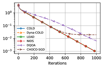
(a) C1

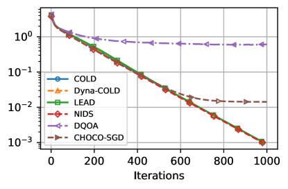
(b) C2

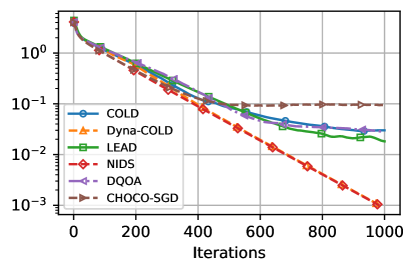
(c) C3

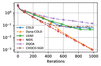
(d) C4

Figure 1: Optimality gap ($\|\nabla f(\bar{\mathbf{x}}^{k})\|$) vs number of iterations for different algorithms with compressors C1-C4.

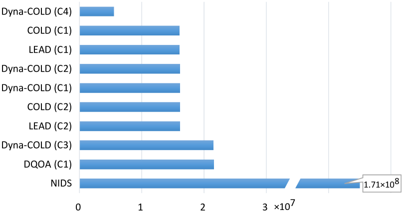
Figure 2: Transmitted bits for different algorithms to reach $\epsilon$-optimal solutions with $\epsilon=10^{-4}$. The algorithm-compressor combinations unable to find an $\epsilon$-optimal solution are not plotted.

V-C Distributed consensus

We compare the uncompressed method in 6, CHOCO-GOSSIP in 7, and our compressed consensus method with scaling (CCS) in 58 on the consensus task. The result is depicted in Fig. 3. We have the following observations:

• CHOCO-GOSSIP and CCS can have similar convergence rates as 6 w.r.t. iterations, which validates Theorem 1.

• CHOCO-GOSSIP cannot converge using C3 and C4, while CCS converges linearly.

• Biased compressors (e.g. C2) can converge faster than the unbiased one (C1) in terms of both iterations and transmitted bits. Moreover, transmitting the minimum number of bits per iteration (C4) does not lead to the minimum overall cost, which is consistent with our theoretical finding.

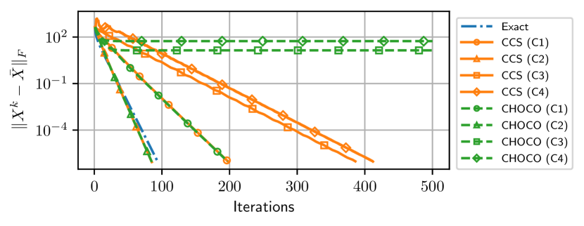
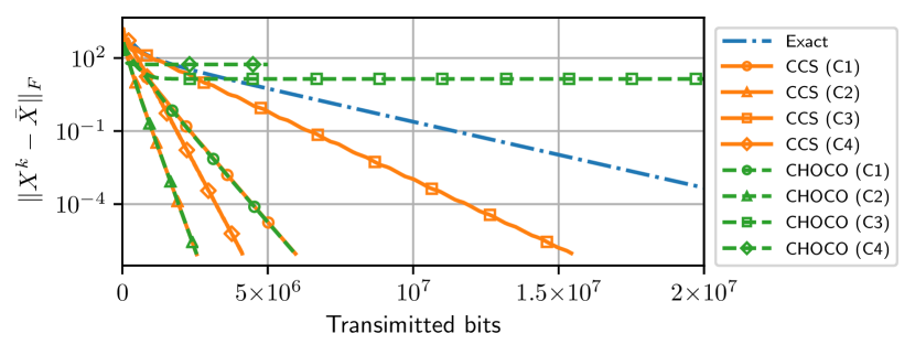
Figure 3: Consensus error vs iterations or transmitted bits. ‘Exact’, ‘CHOCO’, and ‘CCS’ represent the algorithms in 6, 7, and 58, respectively.

VI Conclusion

We proposed two novel communication-efficient distributed algorithms based on innovation compression and dynamic scaling, which achieve linear convergence for two broad classes of compressors. Future works may focus on the extensions to the non-convex and stochastic settings.

Appendix A Proof of Theorem 1

The proof depends on several lemmas. Lemma 4 shows the contraction property of the adjacency matrix $W$.

Lemma 4

For any $W$ satisfying Assumption 4 and $\mathbf{x}\in\text{range}(I-W)$, we have $\lambda_{n}(W)\|\mathbf{x}\|^{2}\leq\|\mathbf{x}\|_{W}^{2}\leq\lambda_{2}(W)\|\mathbf{x}\|^{2}$.

Proof:

By Assumption 4, the eigenvalue 1 is the only eigenvalue of $W$ with magnitude 1, and the corresponding eigenvector is ${\mathbf{1}}_{n}$. Hence, $\text{range}(I-W)=\text{range}(I-\frac{1}{n}{\mathbf{1}}{\mathbf{1}}^{\mathsf{T}})$. Since $\mathbf{x}\in\text{range}(I-W)$, there exists some $\mathbf{d}$ such that $\mathbf{x}=(I-\frac{1}{n}{\mathbf{1}}{\mathbf{1}}^{\mathsf{T}})\mathbf{d}$, which implies that $\|\mathbf{x}\|_{W}^{2}=\mathbf{d}^{\mathsf{T}}(I-\frac{1}{n}{\mathbf{1}}{\mathbf{1}}^{\mathsf{T}})W(I-\frac{1}{n}{\mathbf{1}}{\mathbf{1}}^{\mathsf{T}})\mathbf{d}=\mathbf{d}^{\mathsf{T}}(I-\frac{1}{n}{\mathbf{1}}{\mathbf{1}}^{\mathsf{T}})(W-\frac{1}{n}{\mathbf{1}}{\mathbf{1}}^{\mathsf{T}})(I-\frac{1}{n}{\mathbf{1}}{\mathbf{1}}^{\mathsf{T}})\mathbf{d}=\mathbf{x}^{\mathsf{T}}(W-\frac{1}{n}{\mathbf{1}}{\mathbf{1}}^{\mathsf{T}})\mathbf{x}$. Note that $\lambda_{n}(W)I\preceq W-\frac{1}{n}{\mathbf{1}}{\mathbf{1}}^{\mathsf{T}}\preceq\lambda_{2}(W)I$, and thus the result follows.  

Lemma 5

Under Assumption 4 and let $\bar{X}={\mathbf{1}}\bar{\mathbf{x}}^{\mathsf{T}}$. It holds that

$$\|X^{k}-\bar{X}\|^{2}+\|\widehat{X}^{k}-X^{k-1}\|_{\gamma(W-I)}^{2}$$ (63)

$$=\|X^{k-1}-\bar{X}\|_{I+\gamma(W-I)}^{2}+\|\widehat{X}^{k}-\bar{X}\|_{\gamma(W-I)(I+\gamma(W-I))}^{2}.$$

Proof:

It follows from 7 and Assumption 4 that

$$X^{k}-\bar{X}=X^{k-1}-\bar{X}+\gamma(W-I)\widehat{X}^{k}$$ (64)

$$=X^{k-1}-\bar{X}+\gamma(W-I)(\widehat{X}^{k}-\bar{X}).$$

This implies that

$$\|X^{k}-\bar{X}\|^{2} =\|X^{k-1}-\bar{X}+\gamma(W-I)(\widehat{X}^{k}-\bar{X})\|^{2}$$ (65)

$$=\|X^{k-1}-\bar{X}\|^{2}+\|\widehat{X}^{k}-\bar{X}\|_{\gamma^{2}(W-I)^{2}}^{2}$$

$$\quad+2\langle X^{k-1}-\bar{X},\widehat{X}^{k}-\bar{X}\rangle_{\gamma(W-I)}.$$

Since $\langle\mathbf{a},\mathbf{b}\rangle_{M}=\|\mathbf{a}+\mathbf{b}\|_{M}^{2}-\|\mathbf{a}\|_{M}^{2}-\|\mathbf{b}\|_{M}^{2}$ for any symmetric matrix $M$, we have

$$2\langle X^{k-1}-\bar{X},\widehat{X}^{k}-\bar{X}\rangle_{\gamma(W-I)}$$ (66)

$$=\|\widehat{X}^{k}-X^{k-1}\|_{\gamma(I-W)}^{2}-\|\widehat{X}^{k}-\bar{X}\|_{\gamma(I-W)}^{2}$$

$$\quad-\|X^{k-1}-\bar{X}\|_{\gamma(I-W)}^{2}$$

which jointly with 65 completes the proof.  

Lemma 6

Under Assumptions 1 and 4, it holds that

$$\mathbb{E}\|\widehat{X}^{k+1}-X^{k}\|^{2}$$ (67)

$$\leq\delta\Big{(}\|\widehat{X}^{k}-X^{k-1}\|_{I-\gamma(W-I)}^{2}+\|X^{k-1}-\bar{X}\|_{\gamma(W-I)}^{2}$$

$$\quad+\|\widehat{X}^{k}-\bar{X}\|_{\gamma(W-I)(\gamma(W-I)-I)}^{2}\Big{)}.$$

Proof:

We have from 7 that

$$\mathbb{E}\|\widehat{X}^{k+1}-X^{k}\|^{2}=\mathbb{E}\|\mathsf{Q}(X^{k}-\widehat{X}^{k})-(X^{k}-\widehat{X}^{k})\|^{2}$$ (68)

$$\leq\delta\|\widehat{X}^{k}-X^{k}\|^{2}=\delta\|\widehat{X}^{k}-X^{k-1}-\gamma(W-I)(\widehat{X}^{k}-\bar{X})\|^{2}$$

$$=\delta\big{(}\|\widehat{X}^{k}-X^{k-1}\|^{2}+2\langle X^{k-1}-\widehat{X}^{k},\widehat{X}^{k}-\bar{X}\rangle_{\gamma(W-I)}$$

$$\quad+\|\widehat{X}^{k}-\bar{X}\|_{\gamma^{2}(W-I)^{2}}^{2}\big{)}$$

$$=\delta\big{(}\|\widehat{X}^{k}-X^{k-1}\|_{I-\gamma(W-I)}^{2}+\|X^{k-1}-\bar{X}\|_{\gamma(W-I)}^{2}$$

$$\quad+\|\widehat{X}^{k}-\bar{X}\|_{\gamma(W-I)(\gamma(W-I)-I)}^{2}\big{)}$$

where the inequality follows from Assumption 1, and the last equality follows from

$$2\langle X^{k-1}-\widehat{X}^{k},\widehat{X}^{k}-\bar{X}\rangle_{\gamma(W-I)}$$ (69)

$$=\|X^{k-1}-\bar{X}\|_{\gamma(W-I)}^{2}-\|X^{k-1}-\widehat{X}^{k}\|_{\gamma(W-I)}^{2}$$

$$\quad-\|\widehat{X}^{k}-\bar{X}\|_{\gamma(W-I)}^{2}.$$

Combining the above completes the proof.  

Proof:

Let $q=\frac{1+\gamma(1-\lambda_{n}(W))}{1-\gamma(1-\lambda_{n}(W))}\delta>\delta$. Multiplying LABEL:eq1_lemma1 by $q$ and then adding it to LABEL:eq1_lemma2, we obtain

$$\|X^{k}-\bar{X}\|_{qI}^{2}+\mathbb{E}\|\widehat{X}^{k+1}-X^{k}\|^{2}$$ (70)

$$\leq\|X^{k-1}-\bar{X}\|_{q(I+\gamma(W-I))+\delta\gamma(W-I)}^{2}$$

$$\quad+\|\widehat{X}^{k}-X^{k-1}\|_{\delta(I-\gamma(W-I))-q\gamma(W-I)}^{2}$$

$$\quad+\|\widehat{X}^{k}-\bar{X}\|_{\gamma(W-I)(qI-\delta I+(q+\delta)\gamma(W-I))}^{2}.$$

For any $\gamma\in(0,(1-\lambda_{n}(W))^{-1})$, it follows from Assumption 4 that $\widetilde{W}=\sqrt{\gamma(I-W)}\succeq 0$. We have

$$\gamma(W-I)(qI-\delta I+(q+\delta)\gamma(W-I))$$ (71)

$$=\frac{2\delta\gamma\widetilde{W}\big{(}(I-W)-(1-\lambda_{n}(W))I\big{)}\widetilde{W}}{1-\gamma(1-\lambda_{n}(W))}\preceq 0.$$

It follows from LABEL:eq1_theo1 that

$$\|X^{k}-\bar{X}\|_{qI}^{2}+\mathbb{E}\|\widehat{X}^{k+1}-X^{k}\|^{2}$$ (72)

$$\leq\|X^{k-1}-\bar{X}\|_{q(I+\gamma(W-I))+\delta\gamma(W-I)}^{2}$$

$$\quad+\|\widehat{X}^{k}-X^{k-1}\|_{\delta(I-\gamma(W-I))-q\gamma(W-I)}^{2}$$

$$\leq\|X^{k-1}-\bar{X}\|_{qI+(q+\delta)\gamma(\lambda_{2}(W)-1)I}^{2}$$

$$\quad+\|\widehat{X}^{k}-X^{k-1}\|_{\delta I-(q+\delta)\gamma(\lambda_{n}(W)-1)I}^{2}$$

$$\leq\sigma\Big{(}\|X^{k-1}-\bar{X}\|_{qI}^{2}+\|\widehat{X}^{k}-X^{k-1}\|^{2}\Big{)}$$

where the second inequality follows from Lemma 4 by noticing that each column of $X^{k-1}-\bar{X}=(I-\frac{1}{n}{\mathbf{1}}{\mathbf{1}}^{\mathsf{T}})X^{k-1}$ belongs to $\text{range}(I-W)$, and $\sigma$ is defined as follows

$$\sigma =\max\Big{\{}1-(1+{\delta}/{q})\gamma(1-\lambda_{2}),\delta+(q+\delta)\gamma(1-\lambda_{n})\Big{\}}$$ (73)

$$=\max\Big{\{}1-\frac{2\gamma(1-\lambda_{2})}{1+\gamma(1-\lambda_{n})},\frac{\delta(1+\gamma(1-\lambda_{n}))}{1-\gamma(1-\lambda_{n})}\Big{\}}$$

$$<1$$

where $\lambda_{2}$ and $\lambda_{n}$ are abbreviations for $\lambda_{2}(W)$ and $\lambda_{n}(W)$, respectively, and the last inequality follows from $\gamma<\frac{1-\delta}{(1+\delta)(1-\lambda_{n}(W))}$. Then, the first part of Theorem 1 follows by taking full expectations on both sides.

Substituting $\gamma=\frac{1-\delta}{(3+\delta)(1-\lambda_{n}(W))}$ into 73, we obtain

$$\sigma =\max\Big{\{}1-\frac{(1-\delta)(1-\lambda_{2}(W))}{2(1-\lambda_{n}(W))},\frac{2\delta}{1+\delta}\Big{\}}$$ (74)

$$=1-\frac{(1-\delta)(1-\lambda_{2}(W))}{2(1-\lambda_{n}(W))}.$$

The desired result follows.  

Appendix B Proofs of Lemmas 2 and 3

B-A Proof of Lemma 2

Proof:

We have

$$Y^{k} \overset{\lx@cref{creftype~refnum}{alg_opt1a}}{=}X^{k}-\gamma\Psi^{k}-\gamma\nabla F^{k}$$ (75)

$$\overset{\lx@cref{creftype~refnum}{alg_opt1a}}{=}Y^{k-1}+X^{k}-X^{k-1}+\gamma(\Psi^{k-1}-\Psi^{k})$$

$$\quad+\gamma(\nabla F^{k-1}-\nabla F^{k})$$

$$\overset{\lx@cref{creftype~refnum}{alg_opt1d}}{=}Y^{k-1}+\gamma(\Psi^{k-1}-2\Psi^{k})-\gamma\nabla F^{k}$$

$$\overset{\text{Lemma}~{}\ref{fixed_point}}{=}Y^{k-1}+\gamma(\Psi^{k-1}-\Psi^{k})-\gamma(\Psi^{k}-\Psi^{\star})$$

$$\qquad-\gamma(\nabla F^{k}-\nabla F^{\star}).$$

Therefore,

$$\mathbb{E}\|\widehat{Y}^{k+1}-Y^{k}\|^{2}$$ (76)

$$\overset{\lx@cref{creftype~refnum}{alg_opt1b}}{=}\mathbb{E}\|\mathsf{Q}(Y^{k}-\widehat{Y}^{k})-(Y^{k}-\widehat{Y}^{k})\|^{2}\leq\delta\|\widehat{Y}^{k}-Y^{k}\|^{2}$$

$$\overset{\lx@cref{creftype~refnum}{eq2_lemma5}}{=}\delta\|\widehat{Y}^{k}-Y^{k-1}+\gamma(\Psi^{k}-\Psi^{\star})+\gamma(\Psi^{k}-\Psi^{k-1})$$

$$\quad+\gamma(\nabla F^{k}-\nabla F^{\star})\|^{2}$$

$$\leq\frac{2\delta}{1+\delta}\|\widehat{Y}^{k}-Y^{k-1}\|^{2}$$

$$\quad+\frac{2\delta\gamma^{2}}{1-\delta}\|\Psi^{k}-\Psi^{\star}+\Psi^{k}-\Psi^{k-1}+\nabla F^{k}-\nabla F^{\star}\|^{2}$$

where the first inequality follows from Assumption 1 and the last inequality used the relation $\|\mathbf{a}+\mathbf{b}\|^{2}\leq(1+c)\|\mathbf{a}\|^{2}+(1+\frac{1}{c})\|\mathbf{b}\|^{2},\forall\mathbf{a},\mathbf{b}$ with $c=\frac{1-\delta}{1+\delta}$.  

B-B Proof of Lemma 3

We need several lemmas first.

Lemma 7

Under Assumptions 1, 4 and 3. The following relation holds for all $k\geq 1$,

$$\|X^{k+1}-X^{\star}\|_{\gamma^{-1}}^{2}+\|\Psi^{k+1}-\Psi^{\star}\|_{\Theta}^{2}$$ (77)

$$=\|X^{k}-X^{\star}\|_{\gamma^{-1}}^{2}+\|\Psi^{k}-\Psi^{\star}\|_{\Theta}^{2}-\|X^{k+1}-X^{k}\|_{\gamma^{-1}}^{2}$$

$$\quad-\|\Psi^{k+1}-\Psi^{k}\|_{\Theta}^{2}-2\langle X^{k}-X^{\star},\nabla F^{k}-\nabla F^{\star}\rangle$$

$$\quad-2\langle\nabla F^{k}-\nabla F^{\star},X^{k+1}-X^{k}\rangle$$

$$\quad+2\langle\Psi^{k+1}-\Psi^{\star},\widehat{Y}^{k+1}-Y^{k}\rangle$$

Proof:

We have

$$\langle\widetilde{\Psi}^{k+1},\widetilde{X}^{k+1}\rangle$$ (78)

$$\overset{\lx@cref{creftype~refnum}{alg_opt1d}}{=}\langle\widetilde{\Psi}^{k+1},X^{k}-\gamma\nabla F^{k}-\gamma\Psi^{k+1}-X^{\star}\rangle$$

$$\overset{\lx@cref{creftype~refnum}{alg_opt1a}}{=}\langle\widetilde{\Psi}^{k+1},Y^{k}+\gamma\Psi^{k}-\gamma\Psi^{k+1}-X^{\star}\rangle$$

$$=\langle\widetilde{\Psi}^{k+1},(I-W)Y^{k}\rangle_{(I-W)^{\dagger}}$$

$$\quad+\langle\widetilde{\Psi}^{k+1},\gamma\Psi^{k}-\gamma\Psi^{k+1}-X^{\star}\rangle$$

$$\overset{\lx@cref{creftype~refnum}{alg_opt1c}}{=}\langle\widetilde{\Psi}^{k+1},\tau^{-1}(\Psi^{k+1}-\Psi^{k})$$

$$\quad-(I-W)(\widehat{Y}^{k+1}-Y^{k})\rangle_{(I-W)^{\dagger}}+\gamma\langle\widetilde{\Psi}^{k+1},\Psi^{k}-\Psi^{k+1}\rangle$$

$$=\langle\widetilde{\Psi}^{k+1},\Psi^{k+1}-\Psi^{k}\rangle_{\Theta}-\langle\widetilde{\Psi}^{k+1},\widehat{Y}^{k+1}-Y^{k}\rangle$$

where we used $\widetilde{\Psi}^{k}\in\text{range}(I-W)$ and hence $\langle\widetilde{\Psi}^{k+1},\mathbf{d}\rangle_{(I-W)^{\dagger}(I-W)}=\langle\widetilde{\Psi}^{k+1},\mathbf{d}\rangle,\forall\mathbf{d}$ and $\langle\widetilde{\Psi}^{k+1},X^{\star}\rangle=0$. Therefore,

$$\langle\widetilde{X}^{k},\nabla F^{k}-\nabla F^{\star}\rangle$$ (79)

$$\overset{\lx@cref{creftype~refnum}{alg_opt1d}}{=}\langle\widetilde{X}^{k},\gamma^{-1}(X^{k}-X^{k+1})-\Psi^{k+1}+\Psi^{\star}\rangle$$

$$=\langle\widetilde{X}^{k},X^{k}-X^{k+1}\rangle_{\gamma^{-1}}-\langle\widetilde{X}^{k+1},\widetilde{\Psi}^{k+1}\rangle$$

$$\quad+\langle X^{k+1}-X^{k},\widetilde{\Psi}^{k+1}\rangle$$

$$\overset{\lx@cref{creftype~refnum}{eq1_lemma6}}{=}\langle\widetilde{\Psi}^{k+1}-\gamma^{-1}(\widetilde{X}^{k}),X^{k+1}-X^{k}\rangle$$

$$\quad-\langle\widetilde{\Psi}^{k+1},\Psi^{k+1}-\Psi^{k}\rangle_{\Theta}+\langle\widetilde{\Psi}^{k+1},\widehat{Y}^{k+1}-Y^{k}\rangle$$

$$\overset{\lx@cref{creftype~refnum}{alg_opt1d}}{=}\langle\nabla F^{k}-\nabla F^{\star}+\gamma^{-1}(\widetilde{X}^{k+1}),X^{k}-X^{k+1}\rangle$$

$$\quad-\langle\widetilde{\Psi}^{k+1},\Psi^{k+1}-\Psi^{k}\rangle_{\Theta}+\langle\widetilde{\Psi}^{k+1},\widehat{Y}^{k+1}-Y^{k}\rangle$$

$$=\langle\widetilde{X}^{k+1},X^{k}-X^{k+1}\rangle_{\gamma^{-1}}+\langle\nabla F^{k}-\nabla F^{\star},X^{k}-X^{k+1}\rangle$$

$$\quad-\langle\widetilde{\Psi}^{k+1},\Psi^{k+1}-\Psi^{k}\rangle_{\Theta}+\langle\widetilde{\Psi}^{k+1},\widehat{Y}^{k+1}-Y^{k}\rangle$$

Using $2\langle\mathbf{a},\mathbf{b}\rangle=\|\mathbf{a}+\mathbf{b}\|^{2}-\|\mathbf{a}\|^{2}-\|\mathbf{b}\|^{2}$, we have

$$2\langle\widetilde{X}^{k},\nabla F^{k}-\nabla F^{\star}\rangle+2\langle\nabla F^{k}-\nabla F^{\star},X^{k+1}-X^{k}\rangle$$ (80)

$$\overset{\lx@cref{creftype~refnum}{eq2_lemma6}}{=}2\langle\widetilde{X}^{k+1},X^{k}-X^{k+1}\rangle_{\gamma^{-1}}+2\langle\widetilde{\Psi}^{k+1},\Psi^{k}-\Psi^{k+1}\rangle_{\Theta}$$

$$\quad+2\langle\widetilde{\Psi}^{k+1},\widehat{Y}^{k+1}-Y^{k}\rangle$$

$$=\|\widetilde{X}^{k}\|_{\gamma^{-1}}^{2}-\|\widetilde{X}^{k+1}\|_{\gamma^{-1}}^{2}-\|X^{k+1}-X^{k}\|_{\gamma^{-1}}^{2}$$

$$\quad+\|\widetilde{\Psi}^{k}\|_{\Theta}^{2}-\|\widetilde{\Psi}^{k+1}\|_{\Theta}^{2}-\|\Psi^{k+1}-\Psi^{k}\|_{\Theta}^{2}$$

$$\quad+2\langle\widetilde{\Psi}^{k+1},\widehat{Y}^{k+1}-Y^{k}\rangle$$

The desired result is obtained.  

Lemma 8

Under Assumption 3, we have for all $X,Y\in\mathbb{R}^{n\times p}$ that

$$\langle X-Y,\nabla F(X)-\nabla F(Y)\rangle$$ (81)

$$\geq\frac{\mu L}{\mu+L}\|X-Y\|^{2}+\frac{1}{\mu+L}\|\nabla F(X)-\nabla F(Y)\|^{2}.$$

Proof:

It follows from Theorem 2.1.12 in [38] that

$$\langle\nabla f_{i}(\mathbf{x})-\nabla f_{i}(\mathbf{y}),\mathbf{x}-\mathbf{y}\rangle$$ (82)

$$\geq\frac{\mu L}{\mu+L}\|\mathbf{x}-\mathbf{y}\|^{2}+\frac{1}{\mu+L}\|\nabla f_{i}(\mathbf{x})-\nabla f_{i}(\mathbf{y})\|^{2},\forall i\in\mathcal{V}.$$

The result then follows directly from the definition of $\nabla F$.  

Proof:

For any symmetric $\Theta$, we have $2\langle\mathbf{a},\mathbf{b}\rangle_{\Theta}=\|\mathbf{a}+\mathbf{b}\|_{\Theta}^{2}-\|\mathbf{a}\|_{\Theta}^{2}-\|\mathbf{b}\|_{\Theta}^{2},\forall\mathbf{a},\mathbf{b}$, and hence

$$2\langle\widetilde{X}^{k},\nabla F^{k}-\nabla F^{\star}\rangle+2\langle\nabla F^{k}-\nabla F^{\star},X^{k+1}-X^{k}\rangle$$ (83)

$$=2\langle\widetilde{X}^{k},\nabla F^{k}-\nabla F^{\star}\rangle$$

$$\quad+\|X^{k+1}-X^{k}+\gamma\nabla F^{k}-\gamma\nabla F^{\star}\|_{\gamma^{-1}}^{2}$$

$$\quad-\|\nabla F^{k}-\nabla F^{\star}\|_{\gamma}^{2}-\|X^{k+1}-X^{k}\|_{\gamma^{-1}}^{2}$$

$$\geq\frac{2\mu L\gamma}{\mu+L}\|\widetilde{X}^{k}\|_{\gamma^{-1}}^{2}-\|X^{k+1}-X^{k}\|_{\gamma^{-1}}^{2}+\|\widetilde{\Psi}^{k+1}\|_{\gamma}^{2}$$

$$\quad+\Big{(}\frac{2\gamma^{-1}}{\mu+L}-I\Big{)}\|\nabla F^{k}-\nabla F^{\star}\|_{\gamma}^{2}$$

where the inequality follows from Lemma 8 and 12c. Therefore,

$$\|\widetilde{X}^{k+1}\|_{\gamma^{-1}}^{2}+\|\widetilde{\Psi}^{k+1}\|_{\Theta}^{2}-2\langle\widetilde{\Psi}^{k+1},\widehat{Y}^{k+1}-Y^{k}\rangle$$ (84)

$$\quad+\|\Psi^{k+1}-\Psi^{k}\|_{\Theta}^{2}$$

$$\overset{\lx@cref{creftype~refnum}{eq3_lemma3}}{=}\|\widetilde{X}^{k}\|_{\gamma^{-1}}^{2}+\|\widetilde{\Psi}^{k}\|_{\Theta}^{2}-\|X^{k+1}-X^{k}\|_{\gamma^{-1}}^{2}$$

$$\quad-2\langle\widetilde{X}^{k},\nabla F^{k}-\nabla F^{\star}\rangle-2\langle\nabla F^{k}-\nabla F^{\star},X^{k+1}-X^{k}\rangle$$

$$\overset{\lx@cref{creftype~refnum}{eq1_lemma9}}{\leq}\Big{(}1-\frac{2\mu L\gamma}{\mu+L}\Big{)}\|\widetilde{X}^{k}\|_{\gamma^{-1}}^{2}-\|\widetilde{\Psi}^{k+1}\|_{\gamma}^{2}$$

$$\quad+\|\widetilde{\Psi}^{k}\|_{\Theta}^{2}+\Big{(}1-\frac{2\gamma^{-1}}{\mu+L}\Big{)}\|\nabla F^{k}-\nabla F^{\star}\|_{\gamma}^{2}$$

The desired result is then obtained.  

Appendix C Proof of Theorem 4

We first show some properties of the norm $\|A\|_{\text{max}}\triangleq\max_{i}\|\mathbf{a}_{i*}\|_{p}$.

Lemma 9

1. For any $A\in\mathbb{R}^{n\times d}$, we have $\|A\|_{\text{max}}\leq\bar{c}\|A\|$ and $\|A\|\leq\underline{c}\|A\|_{\text{max}}$, where $\bar{c}=d^{1/p-1/2}$ and $\underline{c}=\sqrt{n}$ for $p\in[1,2)$, and $\bar{c}=1$ and $\underline{c}=\sqrt{n}d^{1/2-1/p}$ for $p\geq 2$.

2. For any two matrices $A$ and $B$ with compatible sizes, it holds that $\|AB\|_{\text{max}}\leq\|A\|_{\infty}\|B\|_{\text{max}}$.

Proof:

(a) The result follows from the definition of $p$-norm and Hölder’s inequality [34].

(b) The result holds since $\|AB\|_{\text{max}}=\max_{i}\|\mathbf{a}_{i*}B\|_{p}\leq\max_{i}\sum_{j=1}^{n}\|a_{ij}\mathbf{b}_{j*}\|_{p}\leq\max_{i}\|\mathbf{a}_{i*}\|_{1}\max_{j}\|\mathbf{b}_{j*}\|_{p}=\|A\|_{\infty}\|B\|_{\text{max}}$.  

Proof:

We prove the result by mathematical induction. It can be easily checked that 60 holds for $k=0$. Suppose that

$$\|\widehat{X}^{k}-X^{k}\|_{\text{max}} \leq c_{s}\beta^{k}=s^{k},$$ (85)

$$\|X^{k}-\bar{X}\| \leq\|X^{0}-{\mathbf{1}}\bar{\mathbf{x}}^{\mathsf{T}}\|\beta^{k}\leq\varsigma c_{s}\beta^{k}$$

for some $k\geq 0$, where $\bar{X}={\mathbf{1}}\bar{\mathbf{x}}^{\mathsf{T}}$. We have

$$\|\widehat{X}^{k+1}-X^{k}\|_{\text{max}}=\|s^{k}\mathsf{Q}(\Delta^{k}/s^{k})-\Delta^{k}\|_{\text{max}}$$ (86)

$$=s^{k}\|\mathsf{Q}(\Delta^{k}/s^{k})-\Delta^{k}/s^{k}\|_{\text{max}}\leq s^{k}\delta=\delta c_{s}\beta^{k}$$

where the inequality follows from Assumption 2 and (85). Note that $\underline{\beta}<1$, it implies that

$$\|\widehat{X}^{k+1}-X^{k+1}\|_{\text{max}}$$ (87)

$$=\|\widehat{X}^{k+1}-X^{k}+\gamma(I-W)\widehat{X}^{k+1}\|_{\text{max}}$$

$$=\|(I+\gamma(I-W))(\widehat{X}^{k+1}-X^{k})$$

$$\qquad+\gamma(I-W)(X^{k}-\bar{X})\|_{\text{max}}$$

$$\leq(1+c_{W}\gamma)\|\widehat{X}^{k+1}-X^{k}\|_{\text{max}}+c_{W}\bar{c}\gamma\|X^{k}-\bar{X}\|$$

$$\leq\big{(}(1+2\gamma)\delta+2\bar{c}\gamma\varsigma\big{)}c_{s}\beta^{k}$$

$$=\Big{(}\frac{1}{2}+\delta\big{(}\frac{1+2\gamma}{2}+\frac{2\underline{c}\bar{c}\gamma}{\rho}\big{)}\Big{)}c_{s}\beta^{k}\leq c_{s}\beta^{k+1}$$

where $c_{W}=1+\|W\|_{\infty}=2$. The first inequality used Lemma 9 and Assumption 4, and the second inequality follows from (85) and LABEL:eq2_theo5.

Moreover, we have

$$\|X^{k+1}-\bar{X}\|$$ (88)

$$\overset{\lx@cref{creftype~refnum}{alg_con2}}{=}\|X^{k}-\bar{X}+\gamma(W-I)(\widehat{X}^{k+1}-X^{k})$$

$$\qquad+\gamma(W-I)(X^{k}-\bar{X})\|$$

$$=\|(I+\gamma(W-I))(X^{k}-\bar{X})+\gamma(W-I)(\widehat{X}^{k+1}-X^{k})\|$$

$$\leq(1-\gamma\rho)\|X^{k}-\bar{X}\|+2\gamma\underline{c}\|\widehat{X}^{k+1}-X^{k}\|_{\text{max}}$$

where the inequality follows from Lemmas 4 and 9.

Let $\underline{\varsigma}={2\delta\underline{c}}/{\rho}\geq 0$ and $\bar{\varsigma}=\frac{1-(1+2\gamma)\delta}{2\gamma}>0$. We have $\underline{\varsigma}\leq\bar{\varsigma}$ and

$$\varsigma=\frac{1}{2}(\underline{\varsigma}+\bar{\varsigma})=\frac{\delta\underline{c}}{\rho}+\frac{1-(1+2\gamma)\delta}{4\gamma}.$$ (89)

By (85), it follows from LABEL:eq3_theo5 that

$$\|X^{k+1}-\bar{X}\| \leq\Big{(}(1-\gamma\rho)+{2\gamma\underline{c}\delta}/{\varsigma}\Big{)}\varsigma c_{s}\beta^{k}$$ (90)

$$\leq\Big{(}(1-\gamma\rho)+{\gamma\underline{c}\delta}/{\underline{\varsigma}}+{\gamma\underline{c}\delta}/{\bar{\varsigma}}\Big{)}\varsigma c_{s}\beta^{k}$$

$$=\Big{(}1-\frac{\gamma\rho}{2}+\frac{2\delta\gamma^{2}\underline{c}\bar{c}}{1-(1+2\gamma)\delta}\Big{)}\varsigma c_{s}\beta^{k}$$

$$\leq\varsigma c_{s}\beta^{k+1}$$

where the second inequality used the relation $\frac{1}{\varsigma}\leq\frac{1}{2\underline{\varsigma}}+\frac{1}{2\bar{\varsigma}}$. Thus, we have shown that $\|X^{k+1}-\bar{X}\|\leq\|X^{0}-{\mathbf{1}}\bar{\mathbf{x}}^{\mathsf{T}}\|\beta^{k+1}$ and $\|\widehat{X}^{k+1}-X^{k+1}\|_{\text{max}}\leq c_{s}\beta^{k+1}$. Thus, he result holds by using $c_{p}=\bar{c}\underline{c}\leq\sqrt{n}d^{|\frac{1}{2}-\frac{1}{\mathbf{p}}|}$ from Lemma 9.  

Appendix D Proof of Theorem 5

D-A Preliminary lemmas

Lemma 10

Under Assumptions 3, 4 and 2. Let $\{X^{k}\}$ and $\{\Psi^{k}\}$ be generated by 61. The following relation holds,

$$\|X^{k+1}-X^{\star}\|_{\gamma^{-1}}^{2}+\|\Psi^{k+1}-\Psi^{\star}\|_{\Theta+\gamma I}^{2}$$ (91)

$$\quad-2\langle\Psi^{k+1}-\Psi^{\star},\widehat{Y}^{k+1}-Y^{k}\rangle+\|\Psi^{k+1}-\Psi^{k}\|_{\Theta}^{2}$$

$$\leq\Big{(}1-\frac{2\mu L\gamma}{\mu+L}\Big{)}\|X^{k}-X^{\star}\|_{\gamma^{-1}}^{2}+\|\Psi^{k}-\Psi^{\star}\|_{\Theta}^{2}$$

$$\quad+\Big{(}1-\frac{2\gamma^{-1}}{\mu+L}\Big{)}\|\nabla F^{k}-\nabla F^{\star}\|_{\gamma}^{2},\forall k\geq 0$$

Proof:

The proof follows from the same line of that of Lemma 3, and hence we omit it here.  

Lemma 11

Suppose Assumptions 3, 4 and 2 hold. Then, for any $\gamma\in(0,\frac{2}{\mu+L})$ and $\zeta\in(0,\gamma)$, the following relation holds,

$$\|X^{k+1}-X^{\star}\|_{\gamma^{-1}}^{2}+\|\Psi^{k+1}-\Psi^{\star}\|_{\Theta+\gamma I-\zeta I}^{2}+\|\Psi^{k+1}-\Psi^{k}\|_{\Theta}^{2}$$ (92)

$$\leq\nu\Big{(}\|X^{k}-X^{\star}\|_{\gamma^{-1}}^{2}+\|\Psi^{k}-\Psi^{\star}\|_{\Theta+\gamma I-\zeta I}^{2}\Big{)}$$

$$\quad+\zeta^{-1}\underline{c}\|\widehat{Y}^{k+1}-Y^{k}\|_{\text{max}}^{2},\ \forall k\geq 0,$$

where

$$\nu\triangleq\max\Big{\{}1-\frac{2\mu L\gamma}{\mu+L},1-\frac{(\gamma-\zeta)\tau(1-\lambda_{2}(W))}{1-\zeta\tau(1-\lambda_{2}(W))}\Big{\}}<1.$$ (93)

Proof:

It follows from LABEL:eq1_lemma10 in Lemma 10, $\gamma\leq\frac{2}{\mu+L}$, and the Cauchy-Schwarz inequality that

$$\|\widetilde{X}^{k+1}\|_{\gamma^{-1}}^{2}+\|\widetilde{\Psi}^{k+1}\|_{\Theta+\gamma I}^{2}+\|\Psi^{k+1}-\Psi^{k}\|_{\Theta}^{2}$$ (94)

$$\leq\big{(}1-\frac{2\mu L\gamma}{\mu+L}\big{)}\|\widetilde{X}^{k}\|_{\gamma^{-1}}^{2}+\|\widetilde{\Psi}^{k}\|_{\Theta}^{2}$$

$$\quad+\zeta\|\widetilde{\Psi}^{k+1}\|^{2}+\zeta^{-1}\|\widehat{Y}^{k+1}-Y^{k}\|^{2}.$$

Since $\zeta\in(0,\gamma)$, we have

$$\Theta \preceq\frac{\tau^{-1}(1-\lambda_{2}(W))^{-1}-\gamma}{\tau^{-1}(1-\lambda_{2}(W))^{-1}-\zeta}(\Theta+\gamma I-\zeta I)$$ (95)

$$\preceq\Big{(}1-\frac{(\gamma-\zeta)\tau(1-\lambda_{2}(W))}{1-\zeta\tau(1-\lambda_{2}(W))}\Big{)}(\Theta+\gamma I-\zeta I).$$

It then follows from LABEL:eq2_lemma10 and Lemma 9 that

$$\|\widetilde{X}^{k+1}\|_{\gamma^{-1}}^{2}+\|\widetilde{\Psi}^{k+1}\|_{\Theta+\gamma I-\zeta I}^{2}+\|\Psi^{k+1}-\Psi^{k}\|_{\Theta}^{2}$$ (96)

$$\leq\big{(}1-\frac{2\mu L\gamma}{\mu+L}\big{)}\|\widetilde{X}^{k}\|_{\gamma^{-1}}^{2}+\zeta^{-1}\underline{c}\|\widehat{Y}^{k+1}-Y^{k}\|_{\text{max}}^{2}$$

$$\quad+\Big{(}1-\frac{(\gamma-\zeta)\tau(1-\lambda_{2}(W))}{1-\zeta\tau(1-\lambda_{2}(W))}\Big{)}\|\widetilde{\Psi}^{k}\|_{\Theta+\gamma I-\zeta I}^{2}$$

which is the desired result LABEL:eq1_lemma4.

 

Lemma 12

Suppose Assumptions 3, 4 and 2 hold. Let $\tau>0$ and $\widetilde{\tau}\in(0,1)$. If $\gamma\in\big{(}0,\min\{\frac{2}{\mu+L},\frac{1}{L}\sqrt{\frac{\widetilde{\tau}}{1-\widetilde{\tau}}},\frac{\widetilde{\tau}}{\tau(1-\lambda_{n}(W))}\}\big{)}$, then

$$\|\widehat{Y}^{k+1}-Y^{k+1}\|_{\text{max}}^{2}$$ (97)

$$\leq\frac{8\gamma\widetilde{\tau}\Big{(}\|\widetilde{\Psi}^{k+1}\|_{\Theta+\frac{\gamma}{2}I}^{2}+\|\widetilde{X}^{k+1}\|_{\gamma^{-1}}^{2}+\|\Psi^{k}-\Psi^{k+1}\|_{\Theta}^{2}\Big{)}}{(1-\delta)^{2}(1-\widetilde{\tau})}$$

$$\quad+\frac{2}{1+\delta}\|\widehat{Y}^{k+1}-Y^{k}\|_{\text{max}}^{2}$$

Proof:

Let $\xi_{1},\xi_{2},\xi_{3}$ be some positive numbers. We have

$$\|\widehat{Y}^{k+1}-Y^{k+1}\|_{\text{max}}^{2}$$ (98)

$$\overset{\lx@cref{creftype~refnum}{alg_opt2}}{=}\|\widehat{Y}^{k+1}-Y^{k}-\gamma(\Psi^{k}-\Psi^{k+1})$$

$$\quad+\gamma(\Psi^{k+1}-\Psi^{\star})+\gamma(\nabla F^{k+1}-\nabla F^{\star})\|_{\text{max}}^{2}$$

$$\leq(1+\xi_{1})\|\widehat{Y}^{k+1}-Y^{k}\|_{\text{max}}^{2}+(1+\xi_{1}^{-1})(1+\xi_{2})\bar{c}\|\widetilde{\Psi}^{k+1}\|_{\gamma^{2}}^{2}$$

$$\quad+(1+\xi_{1}^{-1})(1+\xi_{2}^{-1})\bar{c}\gamma^{2}\times$$

$$\quad\Big{(}(1+\xi_{3})\|\nabla F^{k+1}-\nabla F^{\star}\|^{2}+(1+\xi_{3}^{-1})\|\Psi^{k}-\Psi^{k+1}\|^{2}\Big{)}$$

$$\overset{\lx@cref{creftype~refnum}{eq_lipschitz}}{\leq}(1+\xi_{1})\|\widehat{Y}^{k+1}-Y^{k}\|_{\text{max}}^{2}+(1+\xi_{1}^{-1})(1+\xi_{2})\bar{c}\gamma\Big{(}\|\widetilde{\Psi}^{k+1}\|_{\gamma}^{2}$$

$$\;+\xi_{2}^{-1}\gamma\big{(}(1+\xi_{3})L^{2}\|\widetilde{X}^{k+1}\|^{2}+(1+\xi_{3}^{-1})\|\Psi^{k}-\Psi^{k+1}\|^{2}\big{)}\Big{)}$$

where the first inequality used the Cauchy-Schwarz inequality three times. Set $\xi_{1}=\xi_{2}={(1-\delta)}/{(1+\delta)}>0$ and $\xi_{3}=\left({\gamma L^{2}(\tau^{-1}(1-\lambda_{n}(W))^{-1}-\gamma)}\right)^{-1}>0$. We have

$$\|\widehat{Y}^{k+1}-Y^{k+1}\|_{\text{max}}^{2}$$ (99)

$$\leq(1+\xi_{1})\|\widehat{Y}^{k+1}-Y^{k}\|_{\text{max}}^{2}+(1+\xi_{1}^{-1})(1+\xi_{2})\bar{c}\gamma\Big{(}\|\widetilde{\Psi}^{k+1}\|_{\gamma}^{2}$$

$$\quad+\frac{\xi_{2}^{-1}\gamma(1+\xi_{3}^{-1})\big{(}\|\widetilde{X}^{k+1}\|_{\gamma^{-2}}^{2}+\|\Psi^{k}-\Psi^{k+1}\|_{\psi-1}^{2}\big{)}}{\psi-1}\Big{)}$$

$$\leq\frac{2\|\widehat{Y}^{k+1}-Y^{k}\|_{\text{max}}^{2}}{1+\delta}$$

$$\quad+(1+\xi_{1}^{-1})(1+\xi_{2})\bar{c}\gamma^{2}\Big{(}(\psi-\frac{1}{2})\|\widetilde{\Psi}^{k+1}\|_{\gamma(\Theta+\frac{\gamma}{2}I)}^{2}$$

$$\quad+\frac{\xi_{2}^{-1}(1+\xi_{3}^{-1})\big{(}\|\widetilde{X}^{k+1}\|^{2}+\|\Psi^{k}-\Psi^{k+1}\|_{\gamma\Theta}^{2}\big{)}}{\gamma(\psi-1)}\Big{)}$$

$$\leq\frac{2\|\widehat{Y}^{k+1}-Y^{k}\|_{\text{max}}^{2}}{1+\delta}$$

$$\quad+\bar{c}\gamma\vartheta\Big{(}\|\widetilde{\Psi}^{k+1}\|_{\Theta+\frac{\gamma}{2}I}^{2}+\|\widetilde{X}^{k+1}\|_{\gamma^{-1}}^{2}+\|\Psi^{k}-\Psi^{k+1}\|_{\Theta}^{2}\Big{)}$$

where $\psi=\tau^{-1}\gamma^{-1}(1-\lambda_{n}(W))^{-1}$ and

$$\vartheta =\gamma\max\Big{\{}(1+\xi_{1}^{-1})(1+\xi_{2})\gamma(\psi-\frac{1}{2}),$$ (100)

$$\qquad\qquad\quad\frac{(1+\xi_{1}^{-1})(1+\xi_{2}^{-1})(1+\xi_{3}^{-1})}{\tau^{-1}(1-\lambda_{n}(W))^{-1}-\gamma}\Big{\}}$$

$$=\max\Big{\{}\frac{4\gamma(\tau^{-1}(1-\lambda_{n}(W))^{-1}-\frac{\gamma}{2})}{1-\delta^{2}},$$

$$\qquad\qquad\frac{4\gamma^{2}L^{2}}{(1-\delta)^{2}}+\frac{4\gamma\tau(1-\lambda_{n}(W))}{(1-\delta)^{2}(1-\gamma\tau(1-\lambda_{n}(W)))}\Big{\}}$$

$$\leq\frac{8\widetilde{\tau}}{(1-\delta)^{2}(1-\widetilde{\tau})}$$

and the last inequality follows from $\gamma\leq\frac{1}{L}\sqrt{\frac{\widetilde{\tau}}{1-\widetilde{\tau}}}$. The desired result follows immediately.  

D-B Proof of Theorem 5

Proof:

We prove the result by mathematical induction. Suppose that $\|\widehat{Y}^{k}-Y^{k}\|_{\text{max}}^{2}\leq c\beta^{k}$ and $\|X^{k}-X^{\star}\|_{\gamma^{-1}}^{2}+\|\Psi^{k}-\Psi^{\star}\|_{\Theta+\frac{\gamma}{2}I}^{2}\leq\widetilde{c}\beta^{k}$. Clearly, it holds when $k=0$. Then, we have from Assumption 2 that

$$\|\widehat{Y}^{k+1}-Y^{k}\|_{\text{max}}^{2}=\|s^{k}\mathsf{Q}(\varDelta^{k}/s^{k})-\varDelta^{k}\|_{\text{max}}^{2}\leq\delta s^{k}=\delta c\beta^{k}.$$ (101)

We have from Lemmas 11 and 12 that

$$\|X^{k+1}-X^{\star}\|_{\gamma^{-1}}^{2}+\|\Psi^{k+1}-\Psi^{\star}\|_{\Theta+\frac{\gamma}{2}I}^{2}$$ (102)

$$\overset{\lx@cref{creftype~refnum}{eq1_lemma4}}{\leq}\nu\widetilde{c}\beta^{k}+2\gamma^{-1}\underline{c}\delta c\beta^{k}$$

and

$$\|\widehat{Y}^{k+1}-Y^{k+1}\|_{\text{max}}^{2}$$ (103)

$$\overset{\lx@cref{creftype~refnum}{eq1_lemma11},\lx@cref{creftype~refnum}{eq1_lemma4}}{\leq}\frac{8\bar{c}\gamma\widetilde{\tau}\nu\widetilde{c}\beta^{k}}{(1-\delta)^{2}(1-\widetilde{\tau})}+\Big{(}\frac{16\widetilde{\tau}\underline{c}\bar{c}}{(1-\delta)^{2}(1-\widetilde{\tau})}+\frac{2}{1+\delta}\Big{)}\delta c\beta^{k}$$

where we have set $\zeta=\frac{\gamma}{2}$ and used the hypothesis and 101.

Define the following two functions:

$$g_{1}(t)\triangleq\nu+2\gamma^{-1}\underline{c}\delta t$$ (104)

$$g_{2}(t)\triangleq\frac{2\delta}{1+\delta}+\frac{16\delta\widetilde{\tau}\underline{c}\bar{c}}{(1-\delta)^{2}(1-\widetilde{\tau})}+\frac{8\bar{c}\gamma\widetilde{\tau}\nu}{t(1-\delta)^{2}(1-\widetilde{\tau})}.$$ (105)

In view of LABEL:eq2_theo3 and LABEL:eq1_theo3, it is sufficient to show that $g_{1}(\varsigma)\leq\beta$ and $g_{2}(\varsigma)\leq\beta$ since $\varsigma=c/\widetilde{c}$. To this end, notice that $0<\varsigma_{1}<\varsigma_{2}$, since

$$\Big{(}\frac{(1-\delta)^{3}(1-\widetilde{\tau})}{1+\delta}-16\delta\widetilde{\tau}\underline{c}\bar{c}\Big{)}(\varsigma_{1}-\varsigma_{2})$$ (106)

$$=8\bar{c}\gamma\widetilde{\tau}-\frac{\gamma(1-\delta)^{3}(1-\widetilde{\tau})(1-\nu)}{2\delta(1+\delta)\underline{c}}\leq 0$$

where we used $\widetilde{\tau}\leq\frac{1}{2}$ and the bounds of $\gamma$ and $\tau$ in Theorem 5.

An important relation is that $g_{1}(\varsigma_{2})=1$ and $g_{2}(\varsigma_{1})=1$, which can be readily checked. Moreover, $g_{1}$ is strictly increasing and $g_{2}$ is strictly decreasing w.r.t. $\varsigma$, and both are convex functions. Therefore, we have

$$g_{1}(\varsigma)<\frac{g_{1}(\varsigma_{1})+g_{1}(\varsigma_{2})}{2}\leq\frac{1+\beta_{1}}{2}\leq\beta$$ (107)

and

$$g_{2}(\varsigma)<\frac{g_{2}(\varsigma_{1})+g_{2}(\varsigma_{2})}{2}\leq\frac{1+\beta_{2}}{2}\leq\beta$$ (108)

where $\beta_{1}=g_{1}(\zeta_{1})=\frac{(1-\delta)^{3}(1-\widetilde{\tau})\nu}{(1-\delta)^{3}(1-\widetilde{\tau})-16\delta\widetilde{\tau}(1+\delta)c_{p}}<1$, $\beta_{2}=g_{2}(\zeta_{2})=\frac{2\delta}{1+\delta}+\frac{16\delta\widetilde{\tau}c_{p}}{(1-\delta)^{2}(1-\nu)(1-\widetilde{\tau})}<1$, and we used $c_{p}=\bar{c}\underline{c}\leq\sqrt{n}d^{|\frac{1}{2}-\frac{1}{\mathbf{p}}|}$. Therefore, we finished the induction.  

Jiaqi Zhang received the B.S. degree in electronic and information engineering from the School of Electronic and Information Engineering, Beijing Jiaotong University, Beijing, China, in 2016. He is currently pursuing the Ph.D. degree at the Department of Automation, Tsinghua University, Beijing, China. His current research interests include networked control systems, distributed optimization and learning, and their applications.

Keyou You (SM’17) received the B.S. degree in Statistical Science from Sun Yat-sen University, Guangzhou, China, in 2007 and the Ph.D. degree in Electrical and Electronic Engineering from Nanyang Technological University (NTU), Singapore, in 2012. After briefly working as a Research Fellow at NTU, he joined Tsinghua University in Beijing, China where he is now a tenured Associate Professor in the Department of Automation. He held visiting positions at Politecnico di Torino, Hong Kong University of Science and Technology, University of Melbourne and etc. His current research interests include networked control systems, distributed optimization and learning, and their applications. Dr. You received the Guan Zhaozhi award at the 29th Chinese Control Conference in 2010 and the ACA (Asian Control Association) Temasek Young Educator Award in 2019. He received the National Science Fund for Excellent Young Scholars in 2017. He is serving as an Associate Editor for the IEEE Transactions on Control of Network Systems, IEEE Transactions on Cybernetics, IEEE Control Systems Letters(L-CSS), Systems & Control Letters.

Lihua Xie (F’07) received the B.E. and M.E. degrees in electrical engineering from Nanjing University of Science and Technology in 1983 and 1986, respectively, and the Ph.D. degree in electrical engineering from the University of Newcastle, Australia, in 1992. Since 1992, he has been with the School of Electrical and Electronic Engineering, Nanyang Technological University, Singapore, where he is currently a professor and Director, Delta-NTU Corporate Laboratory for Cyber-Physical Systems. He served as the Head of Division of Control and Instrumentation from July 2011 to June 2014. He held teaching appointments in the Department of Automatic Control, Nanjing University of Science and Technology from 1986 to 1989 and Changjiang Visiting Professorship with South China University of Technology from 2006 to 2011. His research interests include robust control and estimation, networked control systems, multiagent networks, localization, and unmanned systems. He is an Editor-in-Chief for Unmanned Systems and has served as the Editor of IET Book Series in Control and an Associate Editor for a number of journals including the IEEE Transactions on Automatic Control, Automatica, the IEEE Transactions on Control Systems Technology, IEEE Transactions on Network Control Systems, and the IEEE Transactions on Circuits and Systems-II. He was the IEEE Distinguished Lecturer from January 2012 to December 2014 and an Elected Member of Board of Governors, the IEEE Control System Society from January 2016 to December 2018. He is a Fellow of IFAC and Fellow of Academy of Engineering Singapore.

References

- [1] X. Li and L. Xie, “Dynamic formation control over directed networks using graphical laplacian approach,” IEEE Transactions on Automatic Control, vol. 63, no. 11, pp. 3761–3774, 2018.
- [2] Z. Li, W. Ren, X. Liu, and M. Fu, “Consensus of multi-agent systems with general linear and lipschitz nonlinear dynamics using distributed adaptive protocols,” IEEE Transactions on Automatic Control, vol. 58, no. 7, pp. 1786–1791, 2013.
- [3] J. Zhang, K. You, and K. Cai, “Distributed dual gradient tracking for resource allocation in unbalanced networks,” IEEE Transactions on Signal Processing, vol. 68, pp. 2186–2198, 2020.
- [4] J. Zhang and K. You, “Decentralized stochastic gradient tracking for non-convex empirical risk minimization,” arXiv preprint arXiv:1909.02712, 2019.
- [5] A. Nedić and A. Ozdaglar, “Distributed subgradient methods for multi-agent optimization,” IEEE Transactions on Automatic Control, vol. 54, no. 1, pp. 48–61, 2009.
- [6] W. Shi, Q. Ling, G. Wu, and W. Yin, “EXTRA: An exact first-order algorithm for decentralized consensus optimization,” SIAM Journal on Optimization, vol. 25, no. 2, pp. 944–966, 2015.
- [7] Z. Li, W. Shi, and M. Yan, “A decentralized proximal-gradient method with network independent step-sizes and separated convergence rates,” IEEE Transactions on Signal Processing, vol. 67, no. 17, pp. 4494–4506, 2019.
- [8] A. Nedić, A. Olshevsky, and W. Shi, “Achieving geometric convergence for distributed optimization over time-varying graphs,” SIAM Journal on Optimization, vol. 27, no. 4, pp. 2597–2633, 2017.
- [9] G. Qu and N. Li, “Harnessing smoothness to accelerate distributed optimization,” IEEE Transactions on Control of Network Systems, vol. 5, no. 3, pp. 1245–1260, 2018.
- [10] A. Nedic, A. Olshevsky, A. Ozdaglar, and J. N. Tsitsiklis, “Distributed subgradient methods and quantization effects,” in 2008 47th IEEE Conference on Decision and Control. IEEE, 2008, pp. 4177–4184.
- [11] R. Carli, F. Fagnani, P. Frasca, and S. Zampieri, “Gossip consensus algorithms via quantized communication,” Automatica, vol. 46, no. 1, pp. 70–80, 2010.
- [12] A. Reisizadeh, A. Mokhtari, H. Hassani, and R. Pedarsani, “An exact quantized decentralized gradient descent algorithm,” IEEE Transactions on Signal Processing, vol. 67, no. 19, pp. 4934–4947, 2019.
- [13] H. Li, C. Huang, Z. Wang, G. Chen, and H. G. A. Umar, “Computation-efficient distributed algorithm for convex optimization over time-varying networks with limited bandwidth communication,” IEEE Transactions on Signal and Information Processing over Networks, vol. 6, pp. 140–151, 2020.
- [14] P. Yi and Y. Hong, “Quantized subgradient algorithm and data-rate analysis for distributed optimization,” IEEE Transactions on Control of Network Systems, vol. 1, no. 4, pp. 380–392, 2014.
- [15] T. T. Doan, S. T. Maguluri, and J. Romberg, “Convergence rates of distributed gradient methods under random quantization: A stochastic approximation approach,” IEEE Transactions on Automatic Control, 2020.
- [16] H. Tang, S. Gan, C. Zhang, T. Zhang, and J. Liu, “Communication compression for decentralized training,” Advances in Neural Information Processing Systems, vol. 31, pp. 7652–7662, 2018.
- [17] Y. Lu and C. De Sa, “Moniqua: Modulo quantized communication in decentralized SGD,” in Proceedings of the 37th International Conference on Machine Learning, 2020, pp. 6415–6425.
- [18] H. Taheri, A. Mokhtari, H. Hassani, and R. Pedarsani, “Quantized decentralized stochastic learning over directed graphs,” in International Conference on Machine Learning. PMLR, 2020, pp. 9324–9333.
- [19] C.-S. Lee, N. Michelusi, and G. Scutari, “Finite rate quantized distributed optimization with geometric convergence,” in 2018 52nd Asilomar Conference on Signals, Systems, and Computers. IEEE, 2018, pp. 1876–1880.
- [20] S. Magnússon, H. Shokri-Ghadikolaei, and N. Li, “On maintaining linear convergence of distributed learning and optimization under limited communication,” IEEE Transactions on Signal Processing, vol. 68, pp. 6101–6116, 2020.
- [21] Y. Xiong, L. Wu, K. You, and L. Xie, “Quantized distributed gradient tracking algorithm with linear convergence in directed networks,” arXiv preprint arXiv:2104.03649, 2021.
- [22] Z. Li, Y. Liao, K. Huang, and S. Pu, “Compressed gradient tracking for decentralized optimization with linear convergence,” arXiv preprint arXiv:2103.13748, 2021.
- [23] X. Liu, Y. Li, R. Wang, J. Tang, and M. Yan, “Linear convergent decentralized optimization with compression,” in International Conference on Learning Representations, 2021.
- [24] D. Kovalev, A. Koloskova, M. Jaggi, P. Richtarik, and S. Stich, “A linearly convergent algorithm for decentralized optimization: Sending less bits for free!” in International Conference on Artificial Intelligence and Statistics. PMLR, 2021, pp. 4087–4095.
- [25] A. Koloskova, S. Stich, and M. Jaggi, “Decentralized stochastic optimization and gossip algorithms with compressed communication,” in Proceedings of the 36th International Conference on Machine Learning, 2019, pp. 3478–3487.
- [26] L. Xiao and S. Boyd, “Fast linear iterations for distributed averaging,” Systems & Control Letters, vol. 53, no. 1, pp. 65–78, 2004.
- [27] T. Li, M. Fu, L. Xie, and J. Zhang, “Distributed consensus with limited communication data rate,” IEEE Transactions on Automatic Control, vol. 56, no. 2, pp. 279–292, 2011.
- [28] J. Zhang and K. You, “Linearly convergent distributed optimization methods with compressed innovation,” Submitted to the 60th IEEE Conference on Decision and Control, 2021.
- [29] IEEE, “IEEE standard for floating-point arithmetic,” IEEE Std 754-2019 (Revision of IEEE 754-2008), pp. 1–84, 2019.
- [30] N. Elia and S. K. Mitter, “Stabilization of linear systems with limited information,” IEEE transactions on Automatic Control, vol. 46, no. 9, pp. 1384–1400, 2001.
- [31] D. Alistarh, D. Grubic, J. Li, R. Tomioka, and M. Vojnovic, “QSGD: Communication-efficient SGD via gradient quantization and encoding,” in Advances in Neural Information Processing Systems, 2017, pp. 1709–1720.
- [32] S. U. Stich, J.-B. Cordonnier, and M. Jaggi, “Sparsified SGD with memory,” in Advances in Neural Information Processing Systems, 2018, pp. 4447–4458.
- [33] J. Minguillon and J. Pujol, “JPEG standard uniform quantization error modeling with applications to sequential and progressive operation modes,” Journal of Electronic Imaging, vol. 10, no. 2, pp. 475–485, 2001.
- [34] S. Boyd and L. Vandenberghe, Convex optimization. Cambridge university press, 2004.
- [35] B. D. Anderson and J. B. Moore, Optimal filtering. Courier Corporation, 2012.
- [36] T. C. Aysal, M. J. Coates, and M. G. Rabbat, “Distributed average consensus with dithered quantization,” IEEE Transactions on Signal Processing, vol. 56, no. 10, pp. 4905–4918, 2008.
- [37] J. Xu, Y. Tian, Y. Sun, and G. Scutari, “Distributed algorithms for composite optimization: Unified and tight convergence analysis,” arXiv preprint arXiv:2002.11534, 2020.
- [38] Y. Nesterov, Introductory lectures on convex optimization: A basic course. Springer Science & Business Media, 2013, vol. 87.
- [39] N. J. Higham, Accuracy and stability of numerical algorithms. SIAM, 2002.
- [40] T. T. Doan, S. T. Maguluri, and J. Romberg, “Fast convergence rates of distributed subgradient methods with adaptive quantization,” IEEE Transactions on Automatic Control, vol. 66, no. 5, pp. 2191–2205, 2021.
- [41] D. B. West et al., Introduction to graph theory. Prentice hall Upper Saddle River, NJ, 1996, vol. 2.
- [42] Y. LeCun, “The mnist database of handwritten digits,” http://yann. lecun. com/exdb/mnist/, 1998.