Fast Stencil Computations
using Fast Fourier Transforms

Abstract.

Stencil computations are widely used to simulate the change of state of physical systems across a multidimensional grid over multiple timesteps. The state-of-the-art techniques in this area fall into three groups: cache-aware tiled looping algorithms, cache-oblivious divide-and-conquer trapezoidal algorithms, and Krylov subspace methods.

In this paper, we present two efficient parallel algorithms for performing linear stencil computations. Current direct solvers in this domain are computationally inefficient, and Krylov methods require manual labor and mathematical training. We solve these problems for linear stencils by using DFT preconditioning on a Krylov method to achieve a direct solver which is both fast and general. Indeed, while all currently available algorithms for solving general linear stencils perform ${\Theta}\left({NT}\right)$ work, where $N$ is the size of the spatial grid and $T$ is the number of timesteps, our algorithms perform ${o}\left({NT}\right)$ work.

To the best of our knowledge, we give the first algorithms that use fast Fourier transforms to compute final grid data by evolving the initial data for many timesteps at once. Our algorithms handle both periodic and aperiodic boundary conditions, and achieve polynomially better performance bounds (i.e., computational complexity and parallel runtime) than all other existing solutions.

Initial experimental results show that implementations of our algorithms that evolve grids of roughly $10^{7}$ cells for around $10^{5}$ timesteps run orders of magnitude faster than state-of-the-art implementations for periodic stencil problems, and 1.3$\times$ to 8.5$\times$ faster for aperiodic stencil problems.

Code Repository: https://github.com/TEAlab/FFTStencils

1. Introduction

A stencil is a pattern used to compute the value of a cell in a spatial grid at some time step from the values of nearby cells at previous time steps. A stencil computation [49, 130] applies a given stencil to the cells in a spatial grid for some set number of timesteps. Stencil computations have applications in a variety of fields including fluid dynamics [45, 68, 21], electromagnetics [82, 128, 140, 10], mechanical engineering [113, 127, 111], meteorology [114, 115, 11, 75], cellular automata [123, 102, 122, 94], and image processing [147, 107, 142, 146, 117]. In particular, they are widely used for simulating the change of state of physical systems over time [105, 14, 143, 134].

Due to the importance of stencil computations in scientific computing [108, 41, 59], various methods have been devised to improve their runtime performance on different machine architectures [101, 76, 120, 42, 37]. All currently available stencil compilers [37, 65, 67, 92, 109, 25, 130] that can accept arbitrary linear stencils perform ${\Theta}\left({NT}\right)$ work, where $N$ is the number of cells in the spatial grid and $T$ is the number of timesteps.

In this paper, we present the first ${o}\left({NT}\right)$-work stencil computation algorithms that support general linear stencils and arbitrary boundary conditions. Our algorithms have polynomially lower work than all other known options of equivalent or greater generality.

Problem Specification. Consider a stencil computation to be performed over $T$ timesteps on a $d$-dimensional spatial grid of $N$ cells with initial data $a_{0}[\cdots]$. Cell data at subsequent timesteps are defined via application of the linear stencil $S$ across the grid, formalized as $a_{t+1}=Sa_{t}$, where $a_{t}$ is the spatial grid data at timestep $t$. The stencil must define the value of a grid cell in terms of a fixed size neighborhood containing cells from only the prior timestep. We will not be able to apply the stencil to some cells near the boundaries of the grid; the values of these cells are instead defined via boundary conditions. Our goal is to compute the final grid data $a_{T}$ by evolving the initial data $a_{0}$ for $T$ timesteps.

There are two types of boundary conditions we can use: periodic and aperiodic. If the boundary conditions are periodic, it means that every dimension of the spatial grid wraps around onto itself, so the entire grid forms a torus. In this case modular arithmetic is used for all calculations involving spatial indices, and the stencil alone can be used to update all cells. On the other hand, if the boundary conditions are aperiodic, then the cells at the boundary of the grid have to be computed via some method other than straightforward application of the stencil. In this paper, we consider both types of boundary conditions.

Existing Algorithms. There are a handful of algorithms commonly used for carrying out general stencil computations, and many more designed for solving problems with specific boundary conditions and stencils. Here we will give an overview of algorithms which can be used for computations with arbitrary boundary conditions and linear stencils. It is worth noting that almost none of the following algorithms require stencil linearity.

1. [Looping Algorithms.] It is a simple matter to implement stencil computations using nested loops, as shown in Figure 1. However, such computations suffer from poor data locality and hence are inefficient both in theory and in practice. As can be seen from the pseudocode listing, looping codes require ${\Theta}\left({NT}\right)$ work to evolve a grid of $N$ cells forward $T$ timesteps, assuming that the stencil only uses values from a constant size neighborhood.

Figure 1. Looping code for 1-D stencil computations.

2. [Tiled Looping Algorithms.] Adopting a tiling [12, 24] of the spatial grid is a common way to improve the data locality [152, 150, 151, 153, 23] of looping algorithms. The tiles’ size and shape have a strong influence on the runtime of the algorithm, and generally the best performance is attained when each tile fits into the cache. Most modern multicore machines have a hierarchy of caches; to make better use of the cache hierarchy, loop nests may need to be tiled at multiple levels [77, 42].

The most common framework that can be used to derive tiled looping implementations is the polyhedral model, which uses a set of hyperplanes to partition the grid being solved for. The polyhedral model is extensively used in several code generators [3, 2, 4, 155, 141].

3. [Recursive Divide-and-Conquer Algorithms.] Instead of using a predetermined tiling of the spatial grid, these algorithms recursively break the region to be solved for into multiple smaller subregions. The trapezoidal decomposition algorithm [50, 51, 131] is the most well known divide-and-conquer stencil algorithm. Its recursive approach to tiling allows it to be not only both cache-oblivious [48] and cache-adaptive [17, 16], but also to achieve asymptotic cache performance matching that of an optimally tiled stencil code across all levels of the memory hierarchy in a multicore machine.

4. [Krylov Subspace Methods.] Krylov methods compose a diverse set of mathematical techniques which are extensively used in numerical analysis to find successively better approximations of the exact solution to a stencil problem. Such methods are often used to solve problems for which there is no known direct (tiled-loop or divide-and-conquer) solution technique. Discrete Fourier transforms (DFTs) are frequently used in the analysis [27] and implementations [7, 74, 62] of these methods. Krylov methods that use DFTs in their implementations are very restricted in their applicability, usually applying only to stencils from specific PDEs that benefit from spectral analysis.

There are several limitations of Krylov methods as a whole: $(i)$ their initial design requires nontrivial manual convergence analysis [87, 103, 29], $(ii)$ they are mostly applicable only to very small classes of problems [74, 56, 8], $(iii)$ they generally do not produce exact solutions in finite time, but exhibit a trade-off between runtime and accuracy. Improving this trade-off by finding near-optimal preconditioners [19, 18, 135] is a hard problem [33, 81] in the general case.

These common limitations should not be confused for rules, however: because of their diversity, Krylov methods can take on a variety of useful properties when specially designed. For example, when an optimal preconditioner is selected they can find the exact solution in a finite number of iterations. The algorithms we present in this paper will be partially based on an optimally preconditioned Krylov method that is applicable to a rather large class of stencil problems.

Our FFT-Based Algorithms. The computation $S^{T}a_{0}=a_{T}$ (where $S^{T}$ denotes that the stencil $S$ is applied $T$ times) evolves the initial grid data $a_{0}$ for $T$ timesteps to produce the final data $a_{T}$. As will be seen in Section 4, any method of computing $a_{t+1}=Sa_{t}$ is mathematically equivalent to a product where $S$ is viewed as a matrix and $a_{t}$ as a vector. All existing algorithms which find $a_{T}$ exactly do so by direct computation of $a_{T}=S(S(S(\cdots a_{0})))$, where $S$ is applied for a total of $T$ timesteps, incurring ${\Theta}\left({NT}\right)$ work in the process. The looping, tiled, and recursive algorithms we have described differ only in how they break up this series of matrix-vector products. We will instead evaluate this product by diagonalization and repeated squaring of the stencil matrix $S$.

In this paper, we present two FFT-based stencil algorithms: StencilFFT-P for problems with periodic boundary conditions, and StencilFFT-A for those with aperiodic boundary conditions. Our algorithms are applicable to arbitrary uniform linear stencils across vector-valued fields.

1. [Periodic Stencil Algorithm.] Let the discrete Fourier transform (DFT) matrix be written $\mathcal{F}[i,j]=\omega_{N}^{-ij}/\sqrt{N}$, where $\omega_{N}=e^{2\pi\sqrt{-1}/N}$, and let $\mathcal{F}^{-1}$ be the inverse DFT matrix. We use fast Fourier transforms to compute $a_{T}$ as follows:

$$\framebox{$a_{T}=\mathcal{F}^{-1}(\mathcal{F}S\mathcal{F}^{-1})^{T}\mathcal{F}a_{0}$}$$

where $\mathcal{F}S\mathcal{F}^{-1}$ is a diagonal matrix, and $T$ = #timesteps (not a transposition).

To the best of our knowledge, this is the first time that FFT is being applied directly to the problem of computing integral powers of the circulant [61] stencil matrix $S$ that appears in linear stencil computations, even though there is a strong history of using FFT to improve the efficiency of matrix computations [58, 136, 43].

2. [Aperiodic Stencil Algorithm.] When given aperiodic boundary conditions, we use a recursive divide-and-conquer strategy to solve for the boundary of the spatial grid; StencilFFT-P is used as a subroutine to compute cells whose values are independent of the boundary. This method allows us to compute every timestep of the boundary in serial, yet to skip over computing most timesteps of cells near the middle of the grid.

Before we analyze the complexities of our algorithms briefly described above, we give the performance metrics that will be used.

Performance Metrics. We use the work-span model [39] to analyze the performance of dynamic multithreaded parallel programs. Work $T_{1}(n)$ of an algorithm, where $n$ is the input parameter, denotes the total number of serial computations. Span $T_{\infty}(n)$ of an algorithm, also called critical-path length or depth, denotes the maximum number of operations performed on any single processor when the algorithm is run on a machine with an unbounded number of processors. Our analysis of span is performed according to the binary-forking model [22], in which spawning $n$ threads required ${\Theta}\left({\log n}\right)$ span. This model is stricter than PRAM, so all bounds we give hold in the PRAM model as well. Parallel running time $T_{p}(n)$ of an algorithm when run on $p$ processors under a greedy scheduler is given by $T_{p}(n)={\mathcal{O}}\left({T_{1}(n)/p+T_{\infty}(n)}\right)$. Parallelism of an algorithm is the average amount of work performed in each step of its critical path and is computed as $T_{1}(n)/T_{\infty}(n)$.

Table 1. Complexity bounds for stencil algorithms, where $N=$ spatial grid size, $T=$ #timesteps, and $M=$ cache size. It is important to note that the bounds given for our algorithms are for computations with ${\Theta}\left({1}\right)$-size stencils on $d={\Theta}\left({1}\right)$ dimensional hypercubic grids, and that we have simplified the span of StencilFFT-A by assuming $T={\Omega}\left({\log N\log\log N}\right)$. The nested loop, tiled loop, and D&C algorithms work for both periodic and aperiodic boundary conditions. The span for the tiled loop algorithm is ${\Omega}\left({T\log\log N}\right)$.

Table 2. Performance summary of parallel stencil algorithms on a KNL/SKX node.

Performance Analysis of Our Algorithms. The performance of our periodic and aperiodic stencil algorithms are summarized in Table 2. We see that: $(i)$ Both work and span of StencilFFT-P have only logarithmic dependence on $T$ compared with the linear dependence on $T$ in the existing algorithms. $(ii)$ For a $d$-D problem, StencilFFT-A has work quasilinearly dependent on $(TN^{1-1/d}+N)$, whereas all existing algorithms for general linear stencils perform ${\Theta}\left({NT}\right)$ work – a polynomially greater amount. This asymptotic improvement makes possible stencil computations over much larger spacetime grids.

Although we do not show explicit analysis of cache complexity in this paper, it is worth noting that our algorithms are cache-oblivious [48] and cache-adaptive [17, 16].

Our Contributions. Our key contributions are as follows:
1. [Theory.] We present the first algorithms for general linear stencil computations (for both periodic and aperiodic boundary conditions) with ${o}\left({NT}\right)$ work and low span, achieving polynomial speedups over the best existing stencil algorithms.
2. [Practice.] We experimentally analyze the numerical accuracy and runtime of our algorithms as compared to PLuTo [3] code. Implementations of our algorithms for on the order of $10^{7}$ grid cells and $10^{5}$ timesteps suffer no more loss in accuracy from floating point arithmetic than PluTo code, yet run orders of magnitude faster than the best existing implementations of state-of-the-art algorithms for periodic stencil problems, and 1.3$\times$ to 8.5$\times$ faster for aperiodic stencil problems. This is shown in Table 7. Our code is publicly available at
https://github.com/TEAlab/FFTStencils.

2. Related Work & Its Limitations

There is substantial literature devoted to the applications and analysis of stencils and Discrete Fourier Transforms (DFTs). Here we give a background of the relationship between these two areas and examine some of the limitations which appear in the current approaches to stencil codes.

Discrete Fourier Transforms. DFTs are widely used in numerical analysis, with examples including Von Neumann stability analysis [148, 106] to show validity of numerical schemes, DFT-based preconditioning to optimize Krylov iterations [31, 63, 79], and time-domain analysis to achieve partial solutions of given PDEs [69, 36, 97, 121, 104].

A Fast Fourier Transform (FFT) is an algorithm that quickly computes the DFT of an array. The use of FFTs will be important for our algorithms, as they represent a particularly efficient type of matrix-vector multiplication. Several ${\mathcal{O}}\left({N\log N}\right)$-work FFT algorithms exist [60, 30, 149], the most famous among which is the Cooley-Tukey algorithm [38].

Theorem 2.1 (Cooley-Tukey Algorithm, [38, 48]).

The generic Cooley-Tukey FFT algorithm computes the DFT of an array of size $N$ in ${\Theta}\left({N\log N}\right)$ work, ${\mathcal{O}}\left({\log N\log\log N}\right)$ span, and ${\Theta}\left({N}\right)$ space.

Stencil Problems. Stencils are often used in numerical analysis as discretizations of PDEs, since many simple PDEs have prohibitively complex analytical solutions [110, 46] but allow good numerical approximations with a proper choice of stencil.

There are two major types of methods related to stencils: those for deriving numerical schemes, and those for evolving grid data via a given stencil. A discretization method is a way of converting a PDE, which deals with quantities defined over a continuum, into a stencil, which relates quantities defined over discrete sets of variables. A stencil solver is an algorithm that takes stencils, boundary conditions, and initial data as input and performs stencil computations to output final data. This paper presents a pair of stencil solvers for linear stencils which support, respectively, periodic and aperiodic boundary conditions.

Stencil Solvers. Numerical results from stencils are obtained through two primary paths: direct solvers and Krylov methods [118, 70].

Direct solvers are those which find the solution to a stencil problem in a finite number of steps. They often involve feeding the stencil into a stencil compiler such as PLuTo [25], Pochoir [130], or Devito [91], which will output optimized code to compute the action of the stencil across some prespecified grid of initial data for multiple timesteps. Cutting-edge stencil code generators feature many improvements over simple looping algorithms, including better cache efficiency [49, 85], parallelism [83], and low-level compiler optimizations. These systems all perform the same set of updates on the stencil grid, although they vary in the order that these updates are performed. In general they make no use of FFTs.

Krylov subspace methods produce successively better approximations of the exact solution to a given stencil problem. Krylov solvers are often used to solve problems for which there is no known direct solution technique. It is common for DFTs to be used either in the analysis [27] or implementations [7, 74, 62] of Krylov subspace methods, as Fourier analysis is useful for proving scheme stability [32, 156] and convergence rates [57], and DFT matrices are good preconditioners [44] for a large class of matrix equations [26]. In some instances choosing the DFT matrix as a Krylov preconditioner can even convert an approximate solver into a direct one [69, 54]. Krylov subspace methods generally do not produce exact solutions in finite time, but exhibit a trade-off between runtime and accuracy.

Limitations of Current Methods for Stencil Problems.

(1) Manual Analysis. Krylov subspace methods are often accompanied by a mathematically nontrivial convergence analysis [87, 103, 29]; this requires human labor for every new method developed. Since this analysis is not automated [64, 99, 53], the quantity of time it takes varies widely from case to case. Also, the requirement of mathematical rigour strongly discourages the development of unnecessarily general Krylov methods, thus those in the literature usually only apply to specific stencils [9, 93, 56, 8] in order to simplify analysis.

(2) Specialization. The methods [121, 74, 56, 8] published in most of the existing literature on computation with numerical schemes are only applicable to very small classes of problems. DFT preconditioning for Krylov iterations has been used for specific stencils before [72, 52, 124]. However, these techniques have not been generalized to work for higher dimensional grids with general linear stencils.

(3) Inexact Solution. Krylov methods often cannot produce exact solutions, even in the absence of floating-point rounding errors. Using them optimally and reliably thus requires expertise in numerical analysis [137, 70], as well as for substantial effort to be put into uncertainty quantification [89, 86].

(4) Nonoptimal Computational Complexity. All currently available code compilers [37, 65, 67, 92, 109, 25, 130] generate code which has linear work complexity in the number of grid cells and number of time steps to compute, no matter what stencil they are given. Improving this bound has not been addressed in the literature, even when only considering linear stencils.

We show in this paper that when dealing with linear stencils it is possible to produce code that has significantly better asymptotic performance.

(5) No Support for Implicit Stencils. Direct solvers for stencil problems usually do not support implicit stencils; stencil compilers in particular are weak in this respect. Neither Pochoir, PLuTo, nor Devito can be used for directly evolving data via an implicit stencil. This is a significant limitation, as several important stencils are implicit [6, 80, 100, 115, 40, 138].

Significance of This Paper. Current direct solvers for general linear stencil computations are inefficient, and Krylov methods require manual labor and mathematical training. We solve these problems for linear stencils by using DFT preconditioning on a Krylov method to achieve a direct solver which is both fast and general.

3. Applicability of Our Algorithms

In this section, we describe the classes of stencil problems on which our FFT-based stencil algorithms do or do not apply.

Supported Stencil Types. Our algorithms are most directly applicable to homogeneous linear stencils across vector-valued fields. A homogeneous stencil is one that does not vary across the entire spatial grid, and by vector-valued fields we mean we allow each cell value across the spatial grid to be treated as a vector.

All homogeneous linear PDEs can be discretized into supported stencils by using a finite difference approximation [71]. Thus all numerical results for these linear PDEs that were previously reached via analytically-motivated numerical schemes, including those set in the Fourier domain [97, 95], can easily be reached computationally by our algorithms.

It is noteworthy that we support both explicit and implicit linear stencils, and also that vector-valued fields can be used to enable stencils that are dependent on more than one previous timestep. In addition, vector-valued fields allow us to support certain types of inhomogeneity, as mentioned at the end of this section.

Linear stencils are quite common in computational numerics. In fact, the majority of stencils currently used to benchmark [112, 3, 25, 23] stencil compilers are linear.

Unsupported Stencil Types. Our algorithms are not applicable to nonlinear stencils. This is because introducing nonlinearity of any sort invalidates our technique of using DFTs to simplify the action of the stencil. Common examples of nonlinearity in stencils include conditionals, i.e. max/min/if-else, and quadratic dependence on cell values. Most discretizations of nonlinear PDEs pass the nonlinearity on to the stencil, so in general our algorithms cannot be used for stencils from nonlinear PDEs.

Our algorithms cannot be applied to inhomogeneous stencils either. There are two ways that a stencil can break homogeneity. The first is spatially, by having the stencil itself be dependent on local field data, such as is used in slope limiter and flux limiter methods [126, 55, 88] and in mixed media problems [119, 133, 34, 154, 132, 144]. The second way to break homogeneity is temporally, i.e. using a stencil that is dependent on time [66, 84], as would arise from the presence of a forcing term in the original PDE being discretized.

However, we note that there are some special types of inhomogeneity our algorithms can handle, such as those arising from forcing terms which are low-order polynomials in time. These are handled by discretizing homogeneous systems of PDEs to mimic the behaviour of a single inhomogenous PDE.

4. Periodic Stencil Algorithm

In this section we present StencilFFT-P, an efficient parallel algorithm for performing stencil computations with periodic boundary conditions using fast Fourier transforms (FFT). We begin by considering explicit linear stencils on one-dimensional spatial grids, after which we give simple extensions to high-dimensional grids, implicit stencils, and grids where cells are vector-valued.

Mathematical Formulation. Suppose we have a spatial grid of data that evolves in time according to some fixed stencil: cells in the grid at time $t$ are updated as a function of some local neighborhood of cell values at recent times before $t$. For simplicity’s sake, we will assume that the spatial grid is one dimensional until Section 4.2.

In this section, we will exclusively consider linear stencils. A linear stencil $\mathbf{S}$ defines future array values $a_{t+1}[0,\ldots,N-1]$ as a linear function of current array values $a_{t}[0,\ldots,N-1]$. We will later allow array values to be higher dimensional, but for now these constraints are enough on their own to make a significant statement about stencils.

An arbitrary linear mapping from arrays of size $N$ to arrays of size $N$ is, by definition, an $N\times N$ matrix, and therefore the update rule can be written $a_{t+1}[i]=\sum_{j}S[i,j]a_{t}[j]$. We will usually omit the indices in formulas like this, writing $a_{t+1}=Sa_{t}$. As shown in Figure 2, on the surface this update rule may look incomplete – since we require $S$ to use the same neighborhood around each point for updates, how should we proceed when the neighborhood extends beyond the bounds of our spatial array? As filling in these cells is exactly the purpose of boundary conditions, it should come as no surprise that in this section the resolution to this difficulty will come in the form of periodicity.

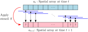
Figure 2. Updating data with a stencil that uses a neighborhood extending one cell to the left and two cells to the right. Cells marked with question marks do not have values defined by the stencil, as the neighborhood required to update them lies partially outside the bounds of the spatial array.

Periodic boundary conditions consist of the rule that $a_{t}[i]=a_{t}[i+N]$, for all $i$. This allows the spatial grid to be extended arbitrarily far in either direction by wrapping around instead of moving outside of the array bounds; in the presence of periodic boundary conditions the spatial grid is effectively a torus, with no clearly defined boundary.

For a stencil to be uniform across space means that it defines updated cell values only from a set of cells which are selected based on their relative location to the cell being updated. For example, if we were to reindex all cells in the spatial array, incrementing them all so the bounds became $1$ and $N$ rather than $0$ and $N-1$, this change of index ought to be invisible to the stencil. Furthermore, in the presence of periodic boundary conditions, this reindexing is equivalent to cyclically shifting the field data $a_{t}$, since we have $a_{t}[0]=a_{t}[N]$.

We mathematically represent the concept of cyclically permuting grid data by introducing the right shift matrix [116] $X$. The array $Xa_{t}$ is defined to be the result of taking the rightmost element $a_{t}[0]$ off and appending it to the left side of the array, i.e. its action on arrays is $(Xa_{t})[i]=a_{t}[i-1]$. An equivalent definition is by $X$’s matrix elements $X[i,j]=\delta_{i,j+1}$, where the Kronecker delta $\delta_{i,j}$ is defined to be 1 if $i=j$ and 0 otherwise, and the arithmetic is understood to be modular with base $N$ in the presence of periodic boundary conditions.

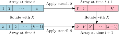
Figure 3. The stencil $S$ does not care where cells are with respect to the start of the array; it only cares about where they are with respect to one another. The shift matrix $X$ does not affect cells’ relative locations, so it does not change the values of the updated cells.

Given that we have periodic boundary conditions and the update rule is fixed across space, the action of our stencils must be invariant under spatial shifts of the grid values. As shown in Figure 3, cyclically permuting $a_{t}$ and then applying $S$ should give the exact same result as applying $S$ and then cyclically permuting $a_{t+1}$. In symbols, we have $SX=XS$, which implies that $S$ must be a circulant matrix [61], satisfying $S[i,j]=S[i-j,0]$. If we name these elements $S[i-j,0]=s_{i-j}$, we can write out the full update equation as follows:

$$\mathop{{}\begin{bmatrix}a_{t+1}[0]\\ a_{t+1}[1]\\ \vdots\\ a_{t+1}[N-2]\\ a_{t+1}[N-1]\end{bmatrix}}_{\textstyle\mathstrut a_{t+1}}=\mathop{{}\begin{bmatrix}s_{0}&s_{N-1}&\cdots&s_{2}&s_{1}\\ s_{1}&s_{0}&s_{N-1}&&s_{2}\\ \vdots&s_{1}&s_{0}&\ddots&\vdots\\ s_{N-2}&&\ddots&\ddots&s_{N-1}\\ s_{N-1}&s_{N-2}&\cdots&s_{1}&s_{0}\end{bmatrix}}_{\textstyle\mathstrut S}\mathop{{}\begin{bmatrix}a_{t}[0]\\ a_{t}[1]\\ \vdots\\ a_{t}[N-2]\\ a_{t}[N-1]\end{bmatrix}}_{\textstyle\mathstrut a_{t}}.$$

A example of this matrix with concrete numbers is constructed in Appendix A.2.

A useful representation of circulant matrices is found through the right shift matrix. Notice that powers of $X$ have the property $(X^{k}a_{t})[i]=a_{t}[i-k]$, which means that their matrix elements are given by $(X^{k})[i,j]=\delta_{i,j+k}$. Thus powers of $X$ allow us to pick out the individual diagonals that appear in circulant matrices; any circulant matrix $S$ can be expanded in terms of shift operators as

$$S=\sum_{i}S[i,0]X^{i},$$

the proof of which is given in Appendix A.6.

The above equation shows that circulant matrices can be uniquely specified by a single one of their columns or rows. We will make use of this fact to avoid performing redundant computations: for all of the algorithms presented in this paper, we will store only the first column of $S$ in memory.

Reformulating the Final Data. We now turn back to the definition of the final data $a_{T}=S^{T}a_{0}$ and the DFT matrix $\mathcal{F}$. Here the exponent $T$ will always denote a matrix power, not a transposition. As before, the DFT matrix has elements $\mathcal{F}[i,j]=\omega_{N}^{-ij}$, where $\omega_{N}=e^{2\pi\sqrt{-1}/N}$ is a primitive $N$th root of unity, and $\mathcal{F}$’s inverse has elements $\mathcal{F}^{-1}[i,j]=\omega_{N}^{ij}/N$. Since we know that $\mathcal{F}^{-1}\mathcal{F}$ is the identity, it can make no difference mathematically to drop it into our equation for the final data:

$$a_{T}=\mathcal{F}^{-1}\mathcal{F}S^{T}\mathcal{F}^{-1}\mathcal{F}a_{0}.$$

Continuing to insert identities and regrouping, we find that $\mathcal{F}S^{T}\mathcal{F}^{-1}=\mathcal{F}S\mathcal{F}^{-1}\mathcal{F}S\mathcal{F}^{-1}\cdots\mathcal{F}S\mathcal{F}^{-1}=(\mathcal{F}S\mathcal{F}^{-1})^{T}$, so we can rewrite our equation as

$$a_{T}=\mathcal{F}^{-1}(\mathcal{F}S\mathcal{F}^{-1})^{T}\mathcal{F}a_{0}.$$

This form of the final data equation points to a remarkably efficient way of computing $a_{T}$. We first apply the convolution theorem [28], which states that if $S$ is a circulant matrix, then $\mathcal{F}S\mathcal{F}^{-1}=\Lambda$ is diagonal. The equation for final data can now be regrouped with $\mathcal{F}S\mathcal{F}^{-1}=\Lambda$ and $\mathcal{F}a_{0}=x$:

(1) $$\boxed{a_{T}=\mathcal{F}^{-1}\Lambda^{T}x.}$$

This equation may appear to be more complicated than what we started with, but really all we have done is made a change of basis into the frequency domain and performed all actions of the stencil there. This will now be shown to be computable with only a couple calls to highly efficient FFTs and some repeated squarings of scalars.

4.1. 1-D Explicit Stencil Algorithm

Let $a_{0}[0,\ldots,N-1]$ be the initial 1-D spatial grid data to be acted on with the stencil $S=\sum_{i}S[i,0]X^{i}$. We will impose periodic boundary conditions; these allow us to benefit from pushing the stencil and initial data into the frequency domain with $\mathcal{F}S\mathcal{F}^{-1}=\Lambda$ and $\mathcal{F}a_{0}=x$. Our goal is to compute the final data

$$a_{T}=S^{T}a_{0}=\mathcal{F}^{-1}\Lambda^{T}x.$$

The prevalent approach to finding $a_{T}$ is currently through iterative applications of the stencil to field data, grouping $S^{T}a_{0}$ into $S(S(\cdots S(a_{0})\cdots))$ and evaluating according to parenthesization. Here we will instead compute a power of the diagonalized stencil $(\mathcal{F}S\mathcal{F}^{-1})^{T}=\Lambda^{T}$ by repeated squaring, after which we will apply it to $\mathcal{F}a_{0}$, giving us $\mathcal{F}S^{T}a_{0}$, from which we can recover $S^{T}a_{0}$ with an inverse FFT.

It is shown in Appendix A.8 that we can write the elements of the diagonal matrix $\Lambda$ as $\Lambda[i,i]=(\mathcal{F}s)[i]$, where $s$ is the column of $S$ that we are storing in memory, i.e. $s[i]=S[i,0]$. Since $\mathcal{F}$ is the DFT matrix, this means that $\Lambda$ can be computed with a single FFT.

Blindly using repeated squaring only allows us to compute $\Lambda^{T}$ when $T$ is an exact power of 2; arbitrary positive integer powers are computed as follows. Let $\sum_{i}b_{i}2^{i}$ be the binary representation of $T$. As we compute successive squares of $\Lambda$, i.e. $\Lambda^{2^{i}}$, we will multiply them into a running total only if $b_{i}=1$. Thus the final result will be

$$\Lambda^{T}=\prod_{i\colon b_{i}=1}\Lambda^{2^{i}}.$$

Since $\Lambda$ is diagonal, elements of the large matrix power $\Lambda^{T}$ can be computed by taking powers of the original elements, $\Lambda^{T}[i,i]=\Lambda[i,i]^{T}$. Evaluating each of these elements in parallel will improve the span of our algorithm.

Wrapping up, we evaluate Equation 1 as follows: we find $x=\mathcal{F}a_{0}$ by applying FFT to the initial data, $\Lambda^{T}x$ by elementwise multiplication, and then $a_{T}$ with an inverse FFT.

We now present the PStencil-1D-FFT algorithm, which efficiently performs stencil computations with periodic boundary conditions by transferring almost all relevant calculations to within the frequency domain. A diagrammatic outline is shown in Figure 5, and the pseudocode is given in Figure 5.

[Step 1. FFT.] We compute $(i)$ $\mathcal{F}S\mathcal{F}^{-1}$ from $S$, and $(ii)$ $\mathcal{F}a_{0}$ from $a_{0}$. Since $S$ is circulant, we know that the FFT of $S$’s first column contains exactly the same information as $\mathcal{F}S\mathcal{F}^{-1}$. Thus for $(i)$ an FFT is applied to the first column of $S$ to get $S$’s eigenvalues; this FFT will be computed for $N$ points, irrespective of how many nonzero coefficients are present in the stencil. Note that only the first column of $S$ is needed here, which is why the rest of $S$ is never constructed or stored in memory. Likewise, for $(ii)$ an FFT is applied to $a_{0}$.
[Step 2. Repeated Squaring.] We compute $\mathcal{F}S^{T}\mathcal{F}^{-1}$ from $\mathcal{F}S\mathcal{F}^{-1}$. Since $\mathcal{F}S\mathcal{F}^{-1}$ is diagonal, the individual elements of $\mathcal{F}S^{T}\mathcal{F}^{-1}=(\mathcal{F}S\mathcal{F}^{-1})^{T}$ can be computed in parallel by performing $\lceil\log T\rceil$ sequential squarings for each element along the principal diagonal of $\mathcal{F}S\mathcal{F}^{-1}$ according to the decomposition of $\Lambda^{T}$ given earlier.
[Step 3. Elementwise Product.] We compute $\mathcal{F}a_{T}$ by taking the product of $\mathcal{F}S^{T}\mathcal{F}^{-1}$ and $\mathcal{F}a_{0}$. As in step 2, every element of $\mathcal{F}a_{T}=(\mathcal{F}S^{T}\mathcal{F}^{-1})(\mathcal{F}a_{0})$ can be computed in parallel, since we are multiplying a vector by a diagonal matrix.
[Step 4. Inverse FFT.] We now compute $a_{T}$ by applying an inverse FFT to $\mathcal{F}a_{T}$.

Theorem 4.1.

StencilFFT-P computes the $T$th timestep of a stencil computation on a periodic grid of $N$ cells in ${\Theta}\left({N\log(NT)}\right)$ work and ${\Theta}\left({\log T+\log N\log\log N}\right)$ span.

Proof.

Theorem follows from bounds given in Table 5. ∎

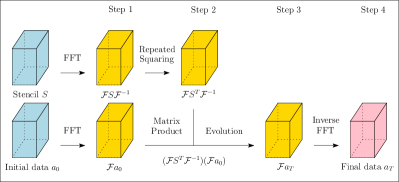
Figure 4. Block diagram of our FFT-based periodic stencil algorithm, which works for all grid sizes in all dimensions.

Figure 5. Arbitrary dimensional periodic stencil algorithm. The Multi-FFT algorithm takes FFTs over every index of the array passed to it. Lines 6-13 compute $\Lambda[j_{1}..j_{d}]^{T}$, where $T$ need not be an exact power of two.

Table 3. Work and span complexity bounds for steps 1-4 of StencilFFT-P. Note that we include thread spawning time from the Binary Forking model in these bounds.

4.2. Generalizations

We now give overviews of some straightforward generalizations of the 1-D algorithm given above. These greatly enhance the scope of stencil problems our algorithm can handle, yet do not require significant conceptual work beyond what we have already presented. There are no changes in the asymptotic complexities of our algorithm when any of these generalizations are applied.

T

Multi-Dimensional Stencils. The first extension of the 1-D version of our algorithm is to support arbitrarily high dimensional grids. The notions involved with solving across a grid of size $\ell_{1}\times\cdots\times\ell_{d}=N$ differ from a 1-D grid only in that we now require indices for every grid dimension; details on the math can be found in Appendix A.1. For our complexity analysis we assume that $d={\Theta}\left({1}\right)$.

Implicit Stencils. The second way we expand the set of problems our algorithm can handle is by giving a method for handling implicit stencils [80]. This is accomplished by mapping them to mathematically equivalent explicit stencils, as explained in Appendix A.4.

Supporting implicit stencils is a significant capability in a stencil solver, as implicit stencils can often be designed to be more stable than explicit ones.

Vector-Valued Fields. The third way we extend our algorithms is to handle vector-valued fields, i.e. fields where the grid data for each cell is an array of fixed length instead of being just a scalar. We allow a set of scalar-valued fields $\{a^{(i)}_{t}\}$ to evolve according to linear stencils as

$$a^{(i)}_{t+1}=\sum_{j}S^{(i,j)}a^{(j)}_{t},$$

where $S^{(i,j)}$ is a circulant stencil matrix describing how $a_{t+1}^{(i)}$ is dependent on $a_{t}^{(j)}$. The details are given in Appendix A.5. It is noteworthy that if there are a constant number of scalar fields $a^{(i)}_{t}$ making up our grid data, then the complexity of finding the final data is only a constant factor greater than if the field were scalar.

Vector-valued grid data allows us to support much larger classes of stencils, such those that are affine or require data from multiple prior timesteps.

5. Aperiodic Stencil Algorithm

In this section we will first consider how introducing aperiodicity into our boundary conditions leads to changes in the final data, then present an algorithm for computing the values of the specific cells that are affected by the aperiodic boundary conditions.

5.1. The Effect of Aperiodicity

Often numerical computations require boundary conditions that are not periodic [20, 15, 98, 129, 73], including well-known classes such as Dirichlet [145] and Von Neumann [90], as well as more exotic options [125]. Indeed, the set of potential aperiodic boundary conditions is extremely diverse. Here we will not attempt to describe how given aperiodic boundary conditions change the final data, but rather what sections of the final data are changed.

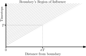
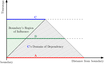
Figure 6. The growth of the boundary’s region of influence over time. Here we assume a stencil that uses $\sigma$ cells in each direction.

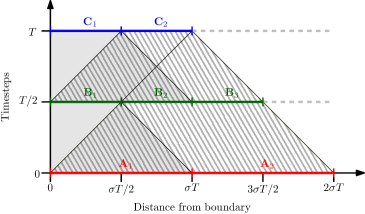
Figure 7. The set of cells relevant to our divide and conquer approach to solving for the boundary’s region of influence. We start with set $A$, from which we will compute set $B$ as an intermediate step, after which we will solve for $C$.

Figure 8. Additional detail on the regions already specified in Figure 8. The dark regions show areas that will be dealt with as RecursiveBoundary subproblems; the light areas can be handled by StencilFFT-P.

The set of cells that are dependent on values from the grid boundary are called the boundary’s region of influence (ROI) [13, 139, 35, 96]. It is common for the boundary’s region of influence to be smaller than the entire spatial grid, as would be the case in a simulation of a large spatial region for a small time period. A cell’s influence on its neighbors is mediated by the stencil, so the larger the stencil is the fewer timesteps it takes for one cell to influence the whole grid.

Consider a stencil with radius $\sigma$, i.e. one which only uses values from a neighborhood extending up to $\sigma$ cells away from its center. After one timestep of a computation based on this stencil, the set of cells which are influenced by aperiodic boundary conditions will be exactly those that are at distance $\sigma$ or less from the grid boundary. After $T$ timesteps, all cells within distance $\sigma T$ of the boundary will be influenced. This suggests that we should visualize how the boundary’s region of influence grows by drawing a diagram in two variables (as in Figure 8), one being time and the other distance from the boundary. Figures of this type will be of significant use to us while describing our aperiodic algorithm.

We now move to our aperiodic algorithm StencilFFT-A, at the core of which is RecursiveBoundary, a divide and conquer technique for correcting the values of the cells in the boundary’s region of influence.

5.2. Correcting Final Values in the Boundary’s Region of Influence

Our aperiodic algorithm breaks up the final data into two regions which will be computed with different methods. The interior region consists of cells whose values will not change no matter what boundary conditions we apply. In particular, periodic boundary conditions would not change the value of these cells. This region will thus be dealt with by using our efficient periodic algorithm. The exterior region is the boundary’s region of influence, made up of cells that are dependent on boundary values.

Since we already know how to solve for the interior region, let us turn our attention to the boundary’s region of influence, which we solve for with a recursive divide and conquer approach. The core idea here will be to perform a time-cut to reduce the number of cells affected by the aperiodic boundary; by splitting one large step into two smaller steps we will be able to use the periodic solver on more space, at the cost of having to compute cell values at an intermediate time.

Figure 8 diagrammatically shows how RecursiveBoundary solves for the boundary region. First all values in region $A$ are used to solve for region $B$, then region $B$ is used to solve for region $C$. These regions can be much smaller than the entire spatial grid, since even though they wrap around the entirety of the boundary, they are only a fixed number of cells thick.

Suppose again that we are performing computations with a stencil of radius $\sigma$. Then set $C$ is the boundary’s region of influence after $T$ timesteps, which includes all cells within distance $\sigma T$ of the boundary. Since we want to be able to fully compute $C$ from $B$ and $B$ from $A$, we must continue to extend our regions as we go $T/2$ steps back for each; $B$ includes everything within $3\sigma T/2$ cells of the boundary, and $A$ includes everything out to a distance of $2\sigma T$. We now refine our naming of these regions, defining subregions $A_{1},A_{2},B_{1},B_{2},B_{3},C_{1}$, and $C_{2}$, whose sizes and locations are shown in Figure 8.

The language we have used up to this point has been dimension-free, in that every statement made has been independent of the number of dimensions in the spatial grid we are performing computations on. Now, to make clear the regions shown in Figures 8 and 8, we will consider what exactly they look like when we make a choice of spatial grid dimension.

In 1-D, when the spatial grid $a[0,\dots,N-1]$ is just a linear array of $N$ cells, the boundary lies to the left of $a[0]$ and to the right of $a[N-1]$. The set of all cells within distance $d$ of the 1-D grid’s boundary is given by the union of $a[0,\dots,d-1]$ and $a[N-d,\dots,N-1]$. For example, the region $C$ is the union of $a[0,\dots,\sigma T-1]$ and $a[N-\sigma T,\dots,N-1]$.

In 2-D things become more complicated, since the boundary of the $n_{1}\times n_{2}$ spatial grid $a[0..(n_{1}-1),0..(n_{2}-1)]$ lies on the outside of the connected set of cells made up of the 1-D subarrays $a[0,0..(n_{2}-1)]$, $a[n_{1}-1,0..(n_{2}-1)]$, $a[0..(n_{1}-1),0]$, and $a[0..(n_{1}-1),n_{2}-1]$. The set of all cells within distance $d$ of the 2-D grid’s boundary is the union of $a[0..(d-1),0..(n_{2}-1)]$, $a[(n_{1}-d)..(n_{1}-1),0..(n_{2}-1)]$, $a[0..(n_{1}-1),0..(d-1)]$, and $a[0..(n_{1}-1),(n_{2}-d)..(n_{2}-1)]$. Note that we are listing some cells twice here, specifically those in the corners of the grid.

Now we are prepared to describe in detail the RecursiveBoundary algorithm for computing the correct values of cells in the boundary’s region of influence. Consider again Figure 8. The RecursiveBoundary algorithm solves for two time-slices which are done sequentially. Each time-slice is divided into two distinct regions: one which is solved for with a periodic solver, and one which is solved for recursively. These two regions are handled in parallel.

1. Solving for $\bm{B}$ from $\bm{A}$. We will begin by feeding data from region $A=A_{1}\cup A_{2}$ into our periodic solver to find values for region $B_{2}\cup B_{3}$. For a $d$-D grid this will take $2d$ calls to the periodic solver. At the same time (in parallel), a recursive call is made to the RecursiveBoundary algorithm with $A_{1}$ as input, writing the output to $B_{1}$. This completes all the values of $B$.

2. Solving for $\bm{C}$ from $\bm{B}$. Now $B=B_{1}\cup B_{2}\cup B_{3}$ is fed into our periodic algorithm to find $C_{2}$, while in parallel we feed $B_{1}\cup B_{2}$ into another recursive call to RecursiveBoundary, which will find the values for $C_{1}$. Thus all cell values in $C=C_{1}\cup C_{2}$ are computed.

The base cases in recursion occur when the only cells to be computed are within a constant distance of the boundary. In this case a standard looping algorithm is applied. Theoretically we can set the cutoff distance to any constant greater than or equal to $\sigma$, but in practice the constant is chosen such that the cost of computing the base case is balanced with the cost of further recursion. See Figure 9 for pseudocode.

Combining our periodic solver for the interior region with this recursive solver for the boundary region gives our aperiodic algorithm StencilFFT-A. A diagrammatic outline of StencilFFT-A is given in Figure 9, and pseudocode is given in Figure 9.

Theorem 5.1.

The StencilFFT-A algorithm can compute the $T$th timestep of a stencil computation on a grid of size $N$ with aperiodic boundary conditions in ${\Theta}\left({bT\log(bT)\log T}\right.$ $\left.{+~{}N\log N}\right)$ work and ${\Theta}\left({T\log b+\log N\log\log N}\right)$ span, where $b$ is the number of grid cells defined by boundary conditions.

The proof is presented in Appendix A.3.

We believe that the bounds we achieve here for work and span are near-optimal (within a polylogarithmic factor) for fully general aperiodic stencil problems. This is because specific choices of nonlinear boundary conditions in combination with linear stencils can result in arbitrary cellular automata being embedded into the boundary of the spatial grid. These automata can be computationally universal (any computation can be mapped to them in a way that preserves time and space complexity), hence the ${\Theta}\left({TN^{1-1/d}}\right)$ (size of the space-time boundary) component in our work complexity and the ${\Theta}\left({T}\right)$ component in our span complexity.

Figure 9. The StencilFFT-A algorithm and the RecursiveBoundary subroutine. The parallel keyword is used here to mark blocks of code which are run on separate processes. Throughout both listings we use a dimension-free indexing notation where $A[a<\mathbf{dist}\leq b]$ represents the set of cells in $A$ that have distance to the boundary in the range $(a,b]$.

6. Experiments

In this section, we present the experimental evaluation of our algorithms as compared with the state-of-the-art stencil codes. Our experimental setup is shown in Table 4.

Table 4. Experimental setup on the Stampede2 Supercomputer [5] using Knights Landing (KNL) Intel Xeon Phi 7250 and Skylake (SKX) Intel Xeon Platinum 8160 nodes.

Benchmarks and Numerical Accuracy. For benchmarks we use a variety of stencil problems including those with periodic and aperiodic boundary conditions and across 1, 2, and 3 dimensions. Our test stencils, primarily drawn from [112] and listed with details in Table 5, are the following: heat1d, heat2d, seidel2d, jacobi2d, heat3d, and 19pt3d (called poisson3d in [112]). We test two primary aspects of our algorithms: numerical accuracy and computational complexity.

To evaluate numerical accuracy we use max relative error against analytical solutions for the heat equation in 1, 2, and 3 dimensions. This is shown in Table 6 against a naïve iterative looping implementations which is numerically equivalent to PLuTo. We see that our algorithms show no significant difference in loss from floating point accuracy when compared against standard looping codes.

Table 5. Benchmark problems with the number of points in the corresponding stencils.

Table 6. Numerical accuracy comparison between our algorithms and looping code. Our analytical solutions were chosen so that the truth values fell within $[0.5,2]$ everywhere in the solution domain.

Table 7. Performance summary of parallel stencil algorithms on a KNL/SKX node.

PLuTo-Generated Stencil Programs. The tiled looping implementations were generated by PLuTo [3] – the state-of-the-art tiled looping code generator. The two main types of tiling methods used for performance comparison are: standard and diamond, whose tiles have the shapes of parallelograms and diamonds, respectively. In the plots, we use diamond and square symbols to denote diamond and standard, respectively. These parallel implementations were run on 68-core KNL and 48-core SKX nodes. The tile sizes were selected via an autotuning phase, exploring sizes from $\{8,16,32\}$ for the outer dimensions and from $\{64,128,512\}$ for the inner-most dimension to ensure that enough vectorization and multithreaded parallelism were exposed by PLuTo, while ensuring the tile footprint neared the cache size.

Our FFT-Based Stencil Programs. Implementations of our FFT-based algorithms use FFT implementations available in the Intel Math Kernel Library (Intel MKL) [1]. In the plots, we use the triangle symbol to represent our FFT-based implementations. The base case sizes used for 1d, 2d, 3d are $128$, $64\times 64$, $16\times 16\times 16$, respectively.

6.1. Periodic Stencil Algorithms

Figure 11 shows runtime, speedup (w.r.t. PLuTo), and scaling plots for our FFT-based periodic stencil algorithm on Intel KNL nodes with Figure 14 in the Appendix showing additional runtime plots. Figure 14 also includes the same set of plots for SKX nodes. We identify the implementations of our algorithms in the plots by prefixing the stencil name with “FFT” while PLuTo-generated implementations are identified by a “PLuTo” prefix.

For 1D, 2D, and 3D stencils we keep the value of $N$ fixed to 1.6M, $8K\times 8K$, and $800\times 800\times 800$, respectively, and vary $T$, where $1$M$=10^{6}$ and $1$K$=10^{3}$.

In all of our 1D and 2D periodic stencil experiments diamond ran faster than standard while in case of 3D standard outperformed diamond. When $N$ is fixed, performance of our algorithm improved over PLuTo’s as $T$ increased, significantly outperforming PLuTo for large $T$, e.g., for seidel2d our algorithm ran around $6000\times$ faster on KNL when $T=10^{5}$. This increase in speedup with the increase of $T$ follows from theoretical predictions. Indeed, theoretical speedup of our algorithm over any existing stencil algorithms is ${\Theta}\left({T/\log T}\right)$ when $N$ is fixed (see Table 2). Hence, the speedup of our algorithm w.r.t. PLuTo-generated codes increased almost linearly with $T$ when $N$ was kept fixed.

Figures 11$(v)$ and 14$(xi)$ show the scalability of our algorithm on KNL and SKX nodes, respectively, when the number of threads is varied. Our implementations are highly parallel and should scale accordingly. However, we use FFT computations that are memory bound – they perform only ${\Theta}\left({N\log{N}}\right)$ work on an input of size ${\Theta}\left({N}\right)$ and thus have very little data reuse. We believe that as a result of this issue, our programs do not scale well beyond 32 threads on KNL and 16 threads on SKX. Indeed, we observe that the FFT and the inverse FFT computations are the scalability bottlenecks of our algorithms.

6.2. Aperiodic Stencil Algorithms

We performed two types of experiments for aperiodic stencils: $(1)$ grid size $N$ was kept fixed while time $T$ was varied, and $(2)$ grid size was set to $N^{1/d}\times\cdots\times N^{1/d}$ and $T=N^{1/d}$ for $d$ dimensions, and $N$ was varied.

Figure 12 shows the runtime (w.r.t. PLuTo) plots of our aperiodic stencil algorithm for both experiments on KNL. Figure 15 in the Appendix includes additional runtime plots for both experiments on KNL. Figures 16 and 17 in the Appendix show the corresponding plots on SKX for Experiments 1 and Experiment 2, respectively.

In Experiment 1, diamond outperformed standard for all stencils except for heat1d on both machines. Our algorithm always ran faster than PLuTo-generated code, reaching speedup factors of 8.5, 2.3–2.4, and 1.3–1.5 for 1D, 2D, and 3D stencils, respectively, on KNL (see Table 7 for details). The corresponding figures on SKX were 5.2, 1.7–4.5, and 1.3–1.4, respectively. Theoretical bounds in Table 2 imply that our algorithm will run around ${\Theta}\left({N^{1/d}/(\log{TN^{1-1/d}})}\right)\log{T}$ factor faster than PLuTo code for any given $N$ and $T$. So, for a fixed $N$, the speedup factor will not increase (may even slightly decrease) with the increase of $T$. The speedup plots match this prediction.

In Experiment 2, diamond ran faster than standard for all stencils except for heat1d and heat3d on KNL and heat1d on SKX. Our algorithm ran up to 5.7, 2.3–2.5, and 1.4–1.8 factor faster than PLuTo-generated code for 1D, 2D, and 3D stencils, respectively, on KNL (see Table 7). The corresponding speedup factors on SKX were 3.3, 1.4–2.6, and 1.4, respectively. Our theoretical prediction for rough speedup factor from the previous paragraph implies that our speedup over PLuTo code will increase with the increase of $N$ which is confirmed by the speedup plots for this experiment. However, the speedup plot of heat2d, seidel2d, and jacobi2d on KNL, as shown in Figure 12$(xi)$ has speedup drops at $N=9000\times 9000$ and $N=15000\times 15000$. Similar performance drops are also observed on SKX nodes (see Figure 17$(viii)$ in the Appendix). We believe that this happens mainly because of a known phenomenon which is the drastic performance variations MKL suffers from when the sizes of the spatial grid dimensions change [78]. This performance drop is also partly due to the changes in the base case kernel size of our implementations resulting from the changes in the grid size.

Figure 10 and Appendix Figure 13 show the scalability plots of our FFT-based aperiodic stencil algorithm on KNL and SKX nodes, respectively. We used $N=1M$, $N=16K\times 16K$, and $N=800\times 800\times 800$ for 1-D, 2-D, and 3-D stencils, respectively, and set $T=N^{1/d}$ for our scalability analysis, where $d$ is the number of dimensions. Our implementations show highly scalable performance on KNL and almost similar scalability for 1D and 2D stencils on SKX.

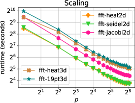
Figure 10. Scalability of our aperiodic algorithms for Experiment 2 on a KNL node.

KNL Node (More plots are given in Figure 14)
$(i)$	$(ii)$	$(iii)$
$(iv)$	$(v)$

Figure 11. Performance comparison of our FFT-based periodic algorithms with the existing best stencil programs.

KNL Node, Experiment 1 (More plots are given in Figures 15, 16, 17, 13)
$(i)$	$(ii)$	$(iii)$
$(iv)$	$(v)$	$(vi)$
KNL Node, Experiment 2 (More plots are given in Figures 15, 16, 17, 13)
$(vii)$	$(viii)$	$(ix)$
$(x)$	$(xi)$	$(xii)$

Figure 12. Performance comparison of our FFT-based aperiodic algorithms with the existing best stencil programs.

7. Conclusion

In this paper, we presented a pair of efficient algorithms based on fast Fourier transforms for performing linear stencil computations with periodic and aperiodic boundary conditions. These are the first high-performing ${o}\left({NT}\right)$-work stencil algorithms of significant generality for computing the spatial grid values at the final timestep from the input grid without explicitly generating values for most of the intermediate timesteps. Our stencil algorithms improve computational complexity and parallel running time bounds over the state-of-the-art stencil algorithms by a polynomial factor. Experimental results show that implementations of our algorithms run orders of magnitude faster than state-of-the-art implementations for periodic stencils and 1.3$\times$ to 8.5$\times$ faster for aperiodic stencils, while exhibiting no significant loss in numerical accuracy from floating point arithmetic.

A few interesting problems that one could aim to solve in the future include: $(1)$ designing efficient algorithms for certain classes of nonlinear stencils and stencils with conditionals, $(2)$ designing low-span algorithms for aperiodic stencils, and $(3)$ designing algorithms to approximate inhomogenous stencils.

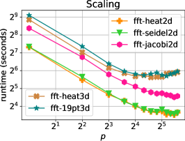
Figure 13. Scalability of our aperiodic algorithms for Experiment 2 on an SKX node.

KNL Node
$(i)$	$(ii)$	$(iii)$
SKX Node
$(iv)$	$(v)$	$(vi)$
$(vii)$	$(viii)$	$(ix)$
$(x)$	$(xi)$

Figure 14. Performance comparison of our FFT-based periodic algorithms with the existing best stencil programs.

KNL Node, Experiment 1
$(i)$	$(ii)$	$(iii)$
KNL Node, Experiment 2
$(iv)$	$(v)$	$(vi)$

Figure 15. Performance comparison of our FFT-based aperiodic algorithms with the existing best stencil programs.

SKX Node, Experiment 1
$(i)$	$(ii)$	$(iii)$
$(iv)$	$(v)$	$(vi)$
$(vii)$	$(viii)$	$(ix)$

Figure 16. Performance comparison of our FFT-based aperiodic algorithms with the existing best stencil programs.

SKX Node, Experiment 2
$(i)$	$(ii)$	$(iii)$
$(iv)$	$(v)$	$(vi)$
$(vii)$	$(viii)$	$(ix)$

Figure 17. Performance comparison of our FFT-based aperiodic algorithms with the existing best stencil programs.

Appendix A Appendix

A.1. Supporting $d$-D Spatial Grids

Throughout this section we will use arguments identical to those given for the 1-D version of StencilFFT-P, but with the modification that whereas the stencil used and grid data used to be indexed by an integer, they will now be indexed by a $d$-D vector $\bm{i}=[i_{1},\dots,i_{d}]$. Let $a_{0}[\bm{i}]$ be the initial data for a grid of size $\ell_{1}\times\cdots\times\ell_{d}=N$ to be acted on by stencil $S=\sum_{\bm{i}}S[\bm{i},\bm{0}]X^{\bm{i}}$, where $X^{\bm{i}}=X_{1}^{i_{1}}\cdots X_{d}^{i_{d}}$ is a shift operator whose action is given by $(X^{\bm{k}}a)[\bm{i}]=a[\bm{i}-\bm{k}]$ and whose matrix elements are $X^{\bm{k}}[\bm{i},\bm{j}]=\delta_{\bm{i},\bm{j}+\bm{k}}$. We have periodic boundary conditions, so $X_{j}$ can be viewed as cyclically permuting the $j$th dimension. Future timesteps are defined with $a_{t+1}=Sa_{t}=S^{t+1}a_{0}$, where matrix multiplications are contractions over the internal vector indices, $(Sa)[\bm{i}]=\sum_{\bm{j}}S[\bm{i},\bm{j}]a[\bm{j}]$.

As with the 1-D case, $S$ is a circulant matrix, so we can apply DFTs over every spatial dimension to diagonalize it. These DFT matrices together make up an operator with elements given by $\mathcal{F}[\bm{i},\bm{j}]=\omega_{\ell_{1}}^{-i_{1}j_{1}}\cdots\omega_{\ell_{d}}^{-i_{d}j_{d}}$ and $\mathcal{F}^{-1}[\bm{i},\bm{j}]=\omega_{\ell_{1}}^{i_{1}j_{1}}\cdots\omega_{\ell_{d}}^{i_{d}j_{d}}/(\ell_{1}\cdots\ell_{d})$. Note of course that by “diagonal” here we mean that $\Lambda[\bm{i},\bm{j}]=(\mathcal{F}S\mathcal{F}^{-1})[\bm{i},\bm{j}]=0$ for all $\bm{i}\neq\bm{j}$. The proof that $\Lambda$ can be found by applying a single Multi-FFT (see Figure 5) over the first column of $S$ is given in Appendix A.8. Here we only restate the result that $\Lambda[\bm{i},\bm{i}]=(\mathcal{F}s)[\bm{i}]$, where $s[\bm{i}]=S[\bm{i},\bm{0}]$.

Switching from 1-D to $d$-D results in the version of the StencilFFT-P algorithm whose pseudocode given in Figure 5 in the main body of this paper. Since Multi-FFT is of equivalent work, span, and serial cache complexity to a standard FFT [47], this version of the StencilFFT-P algorithm is of identical complexity to that already shown in Theorem 4.1.

A.2. Stencil Matrix Example

Suppose we have a 1-D periodic spatial grid of 4 cells, and we want to act on it with a stencil $S$ that computes the new value of a cell according to $a_{t+1}[i]=-2a_{t}[i-1]+a_{t}[i]+3a_{t}[i+1]$. We can write out the update equation in full as

$$\mathop{{}\begin{bmatrix}a_{t+1}[0]\\ a_{t+1}[1]\\ a_{t+1}[2]\\ a_{t+1}[3]\end{bmatrix}}_{\textstyle\mathstrut a_{t+1}}=\mathop{{}\begin{bmatrix}1&3&0&-2\\ -2&1&3&0\\ 0&-2&1&3\\ 3&0&-2&1\end{bmatrix}}_{\textstyle\mathstrut S}\mathop{{}\begin{bmatrix}a_{t}[0]\\ a_{t}[1]\\ a_{t}[2]\\ a_{t}[3]\end{bmatrix}}_{\textstyle\mathstrut a_{t}}.$$

A.3. Proof of Theorem 5.1

Proof.

The complexities for StencilFFT-P have already been given in Theorem 4.1, so here we need only derive the complexities for the RecursiveBoundary computation algorithm.

Let the spatial grid be of size $\ell_{1}\times\cdots\times\ell_{d}=N$, with $d={\Theta}\left({1}\right)$. We bound the number of cells in the boundary’s region of interest by $b\sigma T$, where $b=2N(\ell_{1}^{-1}+\cdots+\ell_{d}^{-1})={\Omega}\left({N^{1-1/d}}\right)$ is the size of the spatial grid’s boundary and $\sigma={\Theta}\left({1}\right)$ is the size of the stencil being applied.
[Work.] At every stage of the divide and conquer algorithm we make two recursive calls and apply the periodic solver to ${\Theta}\left({bT}\right)$ grid cells. This gives us the recurrence

$$T_{1}(T)=\begin{cases}{\Theta}\left({b}\right)&T<c,\\ 2T_{1}(T/2)+{\Theta}\left({bT\log(bT)}\right)&T\geq c,\end{cases}$$

for some positive constant $c$. This gives $T_{1}(T)={\Theta}\left({bT\log(bT)}\right.$
$\left.{\log T}\right)$. Taking into account the ${\Theta}\left({N\log(TN)}\right)$ work that will be done by the periodic solver for the interior region gives a final work bound of ${\Theta}\left({bT\log(bT)\log T+N\log N}\right)$.

[Span.] At every level of recursion, both calls to RecursiveBoundary are done in sequence, but in parallel with the ${\Theta}\left({1}\right)$ associated periodic solver calls. The recurrence for span is thus

$$T_{\infty}(T)=\max\{2T_{\infty}(T/2),c^{\prime}\log T\log\log T\}+{\Theta}\left({\log b}\right),$$

where $c^{\prime}={\Theta}\left({1}\right)$. This gives $T_{\infty}(T)={\Theta}\left({T\log b}\right)$, and incorporating the ${\Theta}\left({\log T+\log N\log\log N}\right)$ span from the periodic solver across the interior region gives a final bound of ${\Theta}\left({T\log b+\log N\log\log N)}\right)$.

∎

A.4. Supporting Implicit Stencils

Here we show how to extend StencilFFT-P to handle stencils which depend implicitly on field data from the timestep which is being computed. This will be done by computing a pseudoinverse after diagonalizing the implicit part of the stencil.

Let $S$ and $Q$ be explicit stencils, and suppose we wish to solve a stencil problem with update equation $Qa_{t+1}=Sa_{t}$. First we diagonalize $\mathcal{F}Q\mathcal{F}^{-1}=\Lambda_{Q}$ and $\mathcal{F}S\mathcal{F}^{-1}=\Lambda_{S}$ by pushing them to the frequency domain, after which we will take the pseudoinverse of $\Lambda_{Q}$, defined as $\Lambda_{Q}^{+}[i,i]=\Lambda_{Q}[i,i]^{-1}$ if $\Lambda_{Q}[i,i]\neq 0$, and 0 otherwise. Now we find a new diagonalized stencil $\Lambda_{R}=\Lambda_{Q}^{+}\Lambda_{S}$. This new stencil $R$ has the following property: if $a_{t+1}=Ra_{t}$, then $Qa_{t+1}=Sa_{t}$.

Thus we can evolve data according to $R$, and the evolved data will satisfy the original implicit stencil equation.

A.5. Supporting Vector Valued Fields

Here we show how to alter our periodic algorithm to handle vector-valued fields, i.e. fields where the grid data for each cell is an array of fixed length instead of being just a scalar. Consider a set of scalar-valued fields $\{a^{(i)}_{t}\}$ which evolve according to linear stencils as

$$a^{(i)}_{t+1}=\sum_{j}S^{(i,j)}a^{(j)}_{t},$$

where $S^{(i,j)}$ is a circulant stencil matrix describing how $a_{t+1}^{(i)}$ is dependent on $a_{t}^{(j)}$. As in the scalar-field case, we can diagonalize all the stencils $S^{(i,j)}$ by moving them to the frequency domain.

Since we now have more than one stencil, we have to revisit our treatment of sequential squaring. Let $\{R^{(i,j)}\}$ be a set of stencils which evolves $a_{t}$ forward $r$ timesteps to $a_{t+r}$,

$$a^{(i)}_{t+r}=\sum_{j}R^{(i,j)}a^{(j)}_{t}.$$

We can find a new set of stencils $\{Q^{(i,j)}\}$ which evolve data forward $2r$ timesteps by reading them off of

$$\sum_{j}Q^{(i,k)}a^{(k)}_{t}=a^{(i)}_{t+2r}=\sum_{j}R^{(i,j)}a^{(j)}_{t+r}=\sum_{j}R^{(i,j)}\sum_{k}R^{(j,k)}a^{(k)}_{t}.$$

This gives the pleasing result that

$$Q^{(i,k)}=\sum_{j}R^{(i,j)}R^{(j,k)},$$

so all we have to do to support vector-valued fields is to swap out our sequential squaring of $\Lambda$ with a sequential squaring of a matrix of stencils.

Furthermore, when there are only a constant number of scalar fields $\{a^{(i)}_{t}\}$ that make up our grid data, the computational complexity of finding $\{Q^{(i,j)}\}$ differs only by a constant factor from squaring $\Lambda$ in our scalar-field version of the algorithm.

As an example of what can be done with vector-valued fields, suppose we want to implement an affine stencil $Aa_{t}=Sa_{t}+c$ on some originally scalar field, where $S$ is a linear stencil and $c$ is a constant. We could then add a spatial field (making the underlying data consist of vectors with 2 elements each) and define $a^{(1)}_{0}=c$, $S^{(1,1)}=S^{(0,1)}=I$, $S^{(1,0)}=0$, and $S^{(0,0)}=A$. This realized the behavior of the affine stencil on $a^{(0)}_{t}$.

A.6. Proof of Shift Matrix Decomposition of Circulant Matrices

Let $S$ be a circulant matrix, and let $X$ be the right shift matrix. Then for any vector $a$, we have

$$(Sa)[i] =\sum_{j}S[i,j]a[j]=\sum_{j}S[i-j,0]a[j]$$

$$=\sum_{j}S[j,0]a[i-j]=\sum_{j}S[j,0](X^{j}a)[i]$$

$$=\left(\left(\sum_{j}S[j,0]X^{j}\right)a\right)[i],$$

which shows that $S=\sum_{i}S[i,0]X^{i}$.

A.7. $\ell$-shell Spatial Grid Decomposition

In the main body of this paper we assume that stencils with some radius $\sigma$ use the values of cells at distance $\sigma$ in any particular direction. However, this is not necessarily the case; one could imagine a stencil that requires a large number of values along one dimension and only a few along another. Upwind stencils also break this pattern, requiring values from very asymmetric neighborhoods of cells.

The concept of region of influence used in our derivation of RecursiveBoundary is itself a sufficient basis for defining the regions $A_{1,2},B_{1,2,3}$, and $C_{1,2}$ shown in Figure 8. Let us define an $\ell$-shell of the boundary of a spatial grid to be the spatial region consisting of all cells that enter the boundary’s region of influence after exactly $\ell$ timesteps. Obviously, there can be only one time $\ell$ when a cell begins to be influenced by the boundary; the set of all $\ell$-shells thus fill the spatial grid without overlapping one another.

To generalize the regions shown in Figure 8 to those for arbitrary stencils, all we have to do is switch the interpretation of the horizontal axis from “distance” to “$\ell$” and scale it by setting $\sigma=1$. This yields an algorithm that is more efficient for upwind schemes and other biased stencils.

A.8. Proof of Eigenvalue-FFT Relation

Expanding the diagonal matrix of eigenvalues $\mathcal{F}A\mathcal{F}^{-1}=\Lambda$ directly gives us

$$\Lambda[i,i] =(\mathcal{F}A\mathcal{F}^{-1})[i,i]=\left(\mathcal{F}\left(\sum_{j}A[j,0]X^{j}\right)\mathcal{F}^{-1}\right)[i,i]$$

$$=\sum_{j}A[j,0](\mathcal{F}X^{j}\mathcal{F}^{-1})[i,i]$$

$$=\sum_{j}A[j,0]\sum_{k}\sum_{\ell}\omega_{N}^{-i\ell}\delta_{\ell,k+j}\omega_{N}^{ki}/N$$

$$=\sum_{j}A[j,0]\sum_{k}\omega_{N}^{-i(k+j)}\omega_{N}^{ki}/N=\sum_{j}\omega_{N}^{-ij}A[j,0]$$

$$=(\mathcal{F}A)[i,0]=(\mathcal{F}a)[i],$$

where in the last line $a$ is the first column of $A$.

References

- [1] Intel math kernel library. https://software.intel.com/content/www/us/en/develop/tools/math-kernel-library.html, Intel MKL.
- [2] Llvm framework for high-level loop and data-locality optimizations. https://polly.llvm.org/, LLVM MKL.
- [3] An automatic parallelizer and locality optimizer for affine loop nests. http://pluto-compiler.sourceforge.net/, Pluto.
- [4] The polyhedral compiler collection. http://web.cs.ucla.edu/~pouchet/software/pocc/, PoCC.
- [5] The stampede2 supercomputing cluster. https://www.tacc.utexas.edu/systems/stampede2, Stampede2.
- [6] V. Acary and B. Brogliato. Implicit euler numerical scheme and chattering-free implementation of sliding mode systems. Systems & Control Letters, 59(5):284–293, 2010.
- [7] O. Andreussi, I. Dabo, and N. Marzari. Revised self-consistent continuum solvation in electronic-structure calculations. The Journal of chemical physics, 136(6):064102, 2012.
- [8] H. Asgharzadeh and I. Borazjani. A newton–krylov method with an approximate analytical jacobian for implicit solution of navier–stokes equations on staggered overset-curvilinear grids with immersed boundaries. Journal of computational physics, 331:227–256, 2017.
- [9] A. Ashrafizadeh, C. Devaud, and N. Aydemir. A jacobian-free newton–krylov method for thermalhydraulics simulations. International Journal for Numerical Methods in Fluids, 77(10):590–615, 2015.
- [10] A. Atangana and J. J. Nieto. Numerical solution for the model of rlc circuit via the fractional derivative without singular kernel. Advances in Mechanical Engineering, 7(10):1687814015613758, 2015.
- [11] R. Avissar and R. A. Pielke. A parameterization of heterogeneous land surfaces for atmospheric numerical models and its impact on regional meteorology. Monthly Weather Review, 117(10):2113–2136, 1989.
- [12] V. Bandishti, I. Pananilath, and U. Bondhugula. Tiling stencil computations to maximize parallelism. In International Conference on High Performance Computing, Networking, Storage and Analysis, pages 1–11, 2012.
- [13] S. L. Barnes. A technique for maximizing details in numerical weather map analysis. Journal of Applied Meteorology and Climatology, 3(4):396–409, 1964.
- [14] T. J. Barth and H. Deconinck. High-order methods for computational physics, volume 9. Springer Science & Business Media, 2013.
- [15] J. H. Beggs, R. J. Luebbers, K. S. Yee, and K. S. Kunz. Finite-difference time-domain implementation of surface impedance boundary conditions. IEEE Transactions on Antennas and propagation, 40(1):49–56, 1992.
- [16] M. A. Bender, E. D. Demaine, R. Ebrahimi, J. T. Fineman, R. Johnson, A. Lincoln, J. Lynch, and S. McCauley. Cache-adaptive analysis. In ACM Symposium on Parallelism in Algorithms and Architectures, pages 135–144, 2016.
- [17] M. A. Bender, R. Ebrahimi, J. T. Fineman, G. Ghasemiesfeh, R. Johnson, and S. McCauley. Cache-adaptive algorithms. In ACM-SIAM Symposium on Discrete Algorithms, 2014.
- [18] M. Benzi and G. H. Golub. A preconditioner for generalized saddle point problems. SIAM Journal on Matrix Analysis and Applications, 26(1):20–41, 2004.
- [19] M. Benzi, M. Ng, Q. Niu, and Z. Wang. A relaxed dimensional factorization preconditioner for the incompressible navier–stokes equations. Journal of Computational Physics, 230(16):6185–6202, 2011.
- [20] S. Bilbao. Modeling of complex geometries and boundary conditions in finite difference/finite volume time domain room acoustics simulation. IEEE Transactions on Audio, Speech, and Language Processing, 21(7):1524–1533, 2013.
- [21] J. Blazek. Computational fluid dynamics: principles and applications. Butterworth-Heinemann, 2015.
- [22] G. E. Blelloch, J. T. Fineman, Y. Gu, and Y. Sun. Optimal parallel algorithms in the binary-forking model. arXiv preprint arXiv:1903.04650, 2019.
- [23] U. Bondhugula, A. Acharya, and A. Cohen. The pluto+ algorithm: A practical approach for parallelization and locality optimization of affine loop nests. ACM Transactions on Programming Languages and Systems, 38(3):1–32, 2016.
- [24] U. Bondhugula, V. Bandishti, and I. Pananilath. Diamond tiling: Tiling techniques to maximize parallelism for stencil computations. IEEE Transactions on Parallel and Distributed Systems, 28(5):1285–1298, 2017.
- [25] U. Bondhugula, A. Hartono, J. Ramanujam, and P. Sadayappan. Pluto: A practical and fully automatic polyhedral program optimization system. In Proceedings of the ACM SIGPLAN 2008 Conference on Programming Language Design and Implementation (PLDI 08), Tucson, AZ (June 2008). Citeseer, 2008.
- [26] R. Borrell, O. Lehmkuhl, F. X. Trias, and A. Oliva. Parallel direct poisson solver for discretisations with one fourier diagonalisable direction. Journal of computational physics, 230(12):4723–4741, 2011.
- [27] J. P. Boyd. Chebyshev and Fourier spectral methods. Courier Corporation, 2001.
- [28] R. N. Bracewell and R. N. Bracewell. The Fourier transform and its applications, volume 31999. McGraw-Hill New York, 1986.
- [29] P. N. Brown and Y. Saad. Convergence theory of nonlinear newton–krylov algorithms. SIAM Journal on Optimization, 4(2):297–330, 1994.
- [30] G. Bruun. z-transform dft filters and fft’s. IEEE Transactions on Acoustics, Speech, and Signal Processing, 26(1):56–63, 1978.
- [31] R. H. Chan, J. G. Nagy, and R. J. Plemmons. Fft-based preconditioners for toeplitz-block least squares problems. SIAM journal on numerical analysis, 30(6):1740–1768, 1993.
- [32] T. F. Chan. Stability analysis of finite difference schemes for the advection-diffusion equation. SIAM journal on numerical analysis, 21(2):272–284, 1984.
- [33] T. F. Chan. An optimal circulant preconditioner for toeplitz systems. SIAM journal on scientific and statistical computing, 9(4):766–771, 1988.
- [34] B.-F. Chen and R. Nokes. Time-independent finite difference analysis of fully non-linear and viscous fluid sloshing in a rectangular tank. Journal of Computational Physics, 209(1):47–81, 2005.
- [35] E. V. Chizhonkov and M. A. Olshanskii. On the domain geometry dependence of the lbb condition. ESAIM: Mathematical Modelling and Numerical Analysis, 34(5):935–951, 2000.
- [36] D. H. Choi and W. J. Hoefer. The finite-difference-time-domain method and its application to eigenvalue problems. IEEE Transactions on Microwave Theory and Techniques, 34(12):1464–1470, 1986.
- [37] M. Christen, O. Schenk, and H. Burkhart. Patus: A code generation and autotuning framework for parallel iterative stencil computations on modern microarchitectures. In 2011 IEEE International Parallel & Distributed Processing Symposium, pages 676–687. IEEE, 2011.
- [38] J. W. Cooley and J. W. Tukey. An algorithm for the machine calculation of complex Fourier series. Mathematics of Computation, 19(90):297–301, 1965.
- [39] T. H. Cormen, C. E. Leiserson, R. L. Rivest, and C. Stein. Introduction to algorithms. MIT press, 2009.
- [40] J. Crank and P. Nicolson. A practical method for numerical evaluation of solutions of partial differential equations of the heat-conduction type. In Mathematical Proceedings of the Cambridge Philosophical Society, volume 43, pages 50–67. Cambridge University Press, 1947.
- [41] G. Dahlquist and Å. Björck. Numerical methods in scientific computing, volume I. SIAM, 2008.
- [42] K. Datta, S. Kamil, S. Williams, L. Oliker, J. Shalf, and K. Yelick. Optimization and performance modeling of stencil computations on modern microprocessors. SIAM review, 51(1):129–159, 2009.
- [43] C. R. Dietrich and G. N. Newsam. Fast and exact simulation of stationary gaussian processes through circulant embedding of the covariance matrix. SIAM Journal on Scientific Computing, 18(4):1088–1107, 1997.
- [44] Y. A. Erlangga, C. W. Oosterlee, and C. Vuik. A novel multigrid based preconditioner for heterogeneous helmholtz problems. SIAM Journal on Scientific Computing, 27(4):1471–1492, 2006.
- [45] J. H. Ferziger, M. Perić, and R. L. Street. Computational methods for fluid dynamics, volume 3. Springer, 2002.
- [46] A. Fokas. On the integrability of linear and nonlinear partial differential equations. Journal of Mathematical Physics, 41(6):4188–4237, 2000.
- [47] M. Frigo and S. G. Johnson. The design and implementation of fftw3. Proceedings of the IEEE, 93(2):216–231, 2005.
- [48] M. Frigo, C. E. Leiserson, H. Prokop, and S. Ramachandran. Cache-oblivious algorithms. In Foundations of Computer Science, pages 285–297, 1999.
- [49] M. Frigo and V. Strumpen. Cache oblivious stencil computations. In Proceedings of the 19th annual international conference on Supercomputing, pages 361–366, 2005.
- [50] M. Frigo and V. Strumpen. Cache oblivious stencil computations. In International conference on Supercomputing, pages 361–366, 2005.
- [51] M. Frigo and V. Strumpen. The cache complexity of multithreaded cache oblivious algorithms. Theory of Computing Systems, 45(2):203–233, 2009.
- [52] J. Fritz, I. Neuweiler, and W. Nowak. Application of fft-based algorithms for large-scale universal kriging problems. Mathematical Geosciences, 41(5):509–533, 2009.
- [53] A. Frommer, K. Lund, D. B. Szyld, et al. Block krylov subspace methods for functions of matrices. 2017.
- [54] V. Fuka. Poisfft–a free parallel fast poisson solver. Applied Mathematics and Computation, 267:356–364, 2015.
- [55] C. F. Gammie, J. C. McKinney, and G. Tóth. Harm: a numerical scheme for general relativistic magnetohydrodynamics. The Astrophysical Journal, 589(1):444, 2003.
- [56] R. Garrappa, I. Moret, and M. Popolizio. Solving the time-fractional schrödinger equation by krylov projection methods. Journal of Computational Physics, 293:115–134, 2015.
- [57] B. Gmeiner, T. Gradl, F. Gaspar, and U. Rüde. Optimization of the multigrid-convergence rate on semi-structured meshes by local fourier analysis. Computers & Mathematics with Applications, 65(4):694–711, 2013.
- [58] I. Gohberg and V. Olshevsky. Fast algorithms with preprocessing for matrix-vector multiplication problems. Journal of Complexity, 10(4):411–427, 1994.
- [59] G. H. Golub, J. M. Ortega, et al. Scientific computing and differential equations: an introduction to numerical methods. Academic press, 1992.
- [60] I. J. Good. The interaction algorithm and practical fourier analysis. Journal of the Royal Statistical Society: Series B (Methodological), 20(2):361–372, 1958.
- [61] R. M. Gray. Toeplitz and circulant matrices: A review. now publishers inc, 2006.
- [62] Y. Guan and I. Novosselov. Two relaxation time lattice boltzmann method coupled to fast fourier transform poisson solver: Application to electroconvective flow. Journal of computational physics, 397:108830, 2019.
- [63] M. H. Gutknecht. A brief introduction to krylov space methods for solving linear systems. In Frontiers of Computational Science, pages 53–62. Springer, 2007.
- [64] S. Guttel, R. Van Beeumen, K. Meerbergen, and W. Michiels. Nleigs: A class of fully rational krylov methods for nonlinear eigenvalue problems. SIAM Journal on Scientific Computing, 36(6):A2842–A2864, 2014.
- [65] B. Hagedorn, L. Stoltzfus, M. Steuwer, S. Gorlatch, and C. Dubach. High performance stencil code generation with lift. In Proceedings of the 2018 International Symposium on Code Generation and Optimization, pages 100–112, 2018.
- [66] W. He and S. S. Ge. Robust adaptive boundary control of a vibrating string under unknown time-varying disturbance. IEEE Transactions on Control Systems Technology, 20(1):48–58, 2011.
- [67] T. Henretty, R. Veras, F. Franchetti, L.-N. Pouchet, J. Ramanujam, and P. Sadayappan. A stencil compiler for short-vector simd architectures. In Proceedings of the 27th international ACM conference on International conference on supercomputing, pages 13–24, 2013.
- [68] C. Hirsch. Numerical computation of internal and external flows: The fundamentals of computational fluid dynamics. Elsevier, 2007.
- [69] R. W. Hockney. A fast direct solution of poisson’s equation using fourier analysis. Journal of the ACM (JACM), 12(1):95–113, 1965.
- [70] I. C. Ipsen and C. D. Meyer. The idea behind krylov methods. The American mathematical monthly, 105(10):889–899, 1998.
- [71] E. Isaacson and H. B. Keller. Analysis of numerical methods. Courier Corporation, 2012.
- [72] P. Janpugdee, P. H. Pathak, P. Mahachoklertwattana, and R. J. Burkholder. An accelerated dft-mom for the analysis of large finite periodic antenna arrays. IEEE transactions on antennas and propagation, 54(1):279–283, 2006.
- [73] H. Johnston and J.-G. Liu. Finite difference schemes for incompressible flow based on local pressure boundary conditions. Journal of Computational Physics, 180(1):120–154, 2002.
- [74] M. Kabel, T. Böhlke, and M. Schneider. Efficient fixed point and newton–krylov solvers for fft-based homogenization of elasticity at large deformations. Computational Mechanics, 54(6):1497–1514, 2014.
- [75] E. Kalnay, M. Kanamitsu, and W. Baker. Global numerical weather prediction at the national meteorological center. Bulletin of the American Meteorological Society, 71(10):1410–1428, 1990.
- [76] S. Kamil, C. Chan, L. Oliker, J. Shalf, and S. Williams. An auto-tuning framework for parallel multicore stencil computations. In 2010 IEEE international symposium on parallel & distributed processing (IPDPS), pages 1–12. IEEE, 2010.
- [77] S. Kamil, P. Husbands, L. Oliker, J. Shalf, and K. Yelick. Impact of modern memory subsystems on cache optimizations for stencil computations. In Proceedings of the 2005 workshop on Memory system performance, pages 36–43, 2005.
- [78] S. Khokhriakov, R. R. Manumachu, and A. Lastovetsky. Performance optimization of multithreaded 2d FFT on multicore processors: Challenges and solution approaches. In 2018 IEEE 25th International Conference on High Performance Computing Workshops (HiPCW). IEEE, Dec. 2018.
- [79] R. C. Kirby and L. Mitchell. Solver composition across the pde/linear algebra barrier. SIAM Journal on Scientific Computing, 40(1):C76–C98, 2018.
- [80] P. E. Kloeden and E. Platen. Higher-order implicit strong numerical schemes for stochastic differential equations. Journal of statistical physics, 66(1):283–314, 1992.
- [81] A. V. Knyazev. Toward the optimal preconditioned eigensolver: Locally optimal block preconditioned conjugate gradient method. SIAM journal on scientific computing, 23(2):517–541, 2001.
- [82] S. Komissarov. Time-dependent, force-free, degenerate electrodynamics. Monthly Notices of the Royal Astronomical Society, 336(3):759–766, 2002.
- [83] M. Kong, R. Veras, K. Stock, F. Franchetti, L.-N. Pouchet, and P. Sadayappan. When polyhedral transformations meet simd code generation. In Proceedings of the 34th ACM SIGPLAN conference on Programming language design and implementation, pages 127–138, 2013.
- [84] T. Konuk and J. Shragge. Modeling full-wavefield time-varying sea-surface effects on seismic data: A mimetic finite-difference approach. Geophysics, 85(2):T45–T55, 2020.
- [85] M. Korch and T. Werner. An in-depth introduction of multi-workgroup tiling for improving the locality of explicit one-step methods for ode systems with limited access distance on gpus. Concurrency and Computation: Practice and Experience, page e6016, 2020.
- [86] P.-S. Koutsourelakis. Accurate uncertainty quantification using inaccurate computational models. SIAM Journal on Scientific Computing, 31(5):3274–3300, 2009.
- [87] A. B. Kuijlaars. Convergence analysis of krylov subspace iterations with methods from potential theory. SIAM review, 48(1):3–40, 2006.
- [88] D. Kuzmin. A vertex-based hierarchical slope limiter for p-adaptive discontinuous galerkin methods. Journal of computational and applied mathematics, 233(12):3077–3085, 2010.
- [89] O. Le Maître and O. M. Knio. Spectral methods for uncertainty quantification: with applications to computational fluid dynamics. Springer Science & Business Media, 2010.
- [90] W. Liao. A high-order adi finite difference scheme for a 3d reaction-diffusion equation with neumann boundary condition. Numerical Methods for Partial Differential Equations, 29(3):778–798, 2013.
- [91] M. Louboutin, M. Lange, F. Luporini, N. Kukreja, P. A. Witte, F. J. Herrmann, P. Velesko, and G. J. Gorman. Devito (v3. 1.0): an embedded domain-specific language for finite differences and geophysical exploration. Geoscientific Model Development, 12(3):1165–1187, 2019.
- [92] F. Luporini, M. Louboutin, M. Lange, N. Kukreja, P. Witte, J. Hückelheim, C. Yount, P. H. Kelly, F. J. Herrmann, and G. J. Gorman. Architecture and performance of devito, a system for automated stencil computation. ACM Transactions on Mathematical Software (TOMS), 46(1):1–28, 2020.
- [93] A. Mang and G. Biros. An inexact newton–krylov algorithm for constrained diffeomorphic image registration. SIAM journal on imaging sciences, 8(2):1030–1069, 2015.
- [94] G. Mendicino, J. Pedace, and A. Senatore. Stability of an overland flow scheme in the framework of a fully coupled eco-hydrological model based on the macroscopic cellular automata approach. Communications in Nonlinear Science and Numerical Simulation, 21(1-3):128–146, 2015.
- [95] K. Moaddy, S. Momani, and I. Hashim. The non-standard finite difference scheme for linear fractional pdes in fluid mechanics. Computers & Mathematics with Applications, 61(4):1209–1216, 2011.
- [96] G. Moretti. The -scheme. Computers & Fluids, 7(3):191–205, 1979.
- [97] D. Mugler and R. Scott. Fast fourier transform method for partial differential equations, case study: The 2-d diffusion equation. Computers & Mathematics with Applications, 16(3):221–228, 1988.
- [98] G. Mur. Absorbing boundary conditions for the finite-difference approximation of the time-domain electromagnetic-field equations. IEEE transactions on Electromagnetic Compatibility, (4):377–382, 1981.
- [99] C. Musco and C. Musco. Randomized block krylov methods for stronger and faster approximate singular value decomposition. Advances in Neural Information Processing Systems, 28:1396–1404, 2015.
- [100] H. N. Najm, P. S. Wyckoff, and O. M. Knio. A semi-implicit numerical scheme for reacting flow: I. stiff chemistry. Journal of Computational Physics, 143(2):381–402, 1998.
- [101] A. Nguyen, N. Satish, J. Chhugani, C. Kim, and P. Dubey. 3.5-d blocking optimization for stencil computations on modern cpus and gpus. In SC’10: Proceedings of the 2010 ACM/IEEE International Conference for High Performance Computing, Networking, Storage and Analysis, pages 1–13. IEEE, 2010.
- [102] U. Nkwunonwo, M. Whitworth, and B. Baily. Urban flood modelling combining cellular automata framework with semi-implicit finite difference numerical formulation. Journal of African Earth Sciences, 150:272–281, 2019.
- [103] Y. Notay and P. S. Vassilevski. Recursive krylov-based multigrid cycles. Numerical Linear Algebra with Applications, 15(5):473–487, 2008.
- [104] V. E. Ostashev, D. K. Wilson, L. Liu, D. F. Aldridge, N. P. Symons, and D. Marlin. Equations for finite-difference, time-domain simulation of sound propagation in moving inhomogeneous media and numerical implementation. The Journal of the Acoustical Society of America, 117(2):503–517, 2005.
- [105] T. Pang. An introduction to computational physics, 1999.
- [106] A. Pereda, L. A. Vielva, A. Vegas, and A. Prieto. Analyzing the stability of the fdtd technique by combining the von neumann method with the routh-hurwitz criterion. IEEE Transactions on Microwave Theory and Techniques, 49(2):377–381, 2001.
- [107] G. Peyré. The numerical tours of signal processing-advanced computational signal and image processing. IEEE Computing in Science and Engineering, 13(4):94–97, 2011.
- [108] W. H. Press, S. A. Teukolsky, W. T. Vetterling, and B. P. Flannery. Numerical recipes 3rd edition: The art of scientific computing. Cambridge university press, 2007.
- [109] J. Ragan-Kelley, C. Barnes, A. Adams, S. Paris, F. Durand, and S. Amarasinghe. Halide: a language and compiler for optimizing parallelism, locality, and recomputation in image processing pipelines. Acm Sigplan Notices, 48(6):519–530, 2013.
- [110] A. Ramani, B. Grammaticos, and T. Bountis. The painlevé property and singularity analysis of integrable and non-integrable systems. Physics Reports, 180(3):159–245, 1989.
- [111] M. Rappaz, M. Bellet, and M. Deville. Numerical modeling in materials science and engineering, volume 32. Springer Science & Business Media, 2010.
- [112] P. S. Rawat, M. Vaidya, A. Sukumaran-Rajam, M. Ravishankar, V. Grover, A. Rountev, L.-N. Pouchet, and P. Sadayappan. Domain-specific optimization and generation of high-performance gpu code for stencil computations. Proceedings of the IEEE, 106(11):1902–1920, 2018.
- [113] L. Renson, G. Kerschen, and B. Cochelin. Numerical computation of nonlinear normal modes in mechanical engineering. Journal of Sound and Vibration, 364:177–206, 2016.
- [114] A. Robert. A stable numerical integration scheme for the primitive meteorological equations. Atmosphere-Ocean, 19(1):35–46, 1981.
- [115] A. Robert. A semi-lagrangian and semi-implicit numerical integration scheme for the primitive meteorological equations. Journal of the Meteorological Society of Japan. Ser. II, 60(1):319–325, 1982.
- [116] G.-C. Rota, D. Kahaner, and A. Odlyzko. On the foundations of combinatorial theory. viii. finite operator calculus. Journal of Mathematical Analysis and Applications, 42(3):684–760, 1973.
- [117] J. C. Russ, J. R. Matey, A. J. Mallinckrodt, and S. McKay. The image processing handbook. Computers in Physics, 8(2):177–178, 1994.
- [118] Y. Saad. Krylov subspace methods on supercomputers. SIAM Journal on Scientific and Statistical Computing, 10(6):1200–1232, 1989.
- [119] H. I. Saleheen and K. T. Ng. New finite difference formulations for general inhomogeneous anisotropic bioelectric problems. IEEE transactions on biomedical engineering, 44(9):800–809, 1997.
- [120] K. Sano, Y. Hatsuda, and S. Yamamoto. Scalable streaming-array of simple soft-processors for stencil computations with constant memory-bandwidth. In 2011 IEEE 19th Annual International Symposium on Field-Programmable Custom Computing Machines, pages 234–241. IEEE, 2011.
- [121] U. Schumann and R. A. Sweet. Fast fourier transforms for direct solution of poisson’s equation with staggered boundary conditions. Journal of Computational Physics, 75(1):123–137, 1988.
- [122] M. Sitko, M. Pietrzyk, and L. Madej. Time and length scale issues in numerical modelling of dynamic recrystallization based on the multi space cellular automata method. Journal of computational science, 16:98–113, 2016.
- [123] J. Somers. Direct simulation of fluid flow with cellular automata and the lattice-boltzmann equation. Applied Scientific Research, 51(1-2):127–133, 1993.
- [124] M. A. Storti, R. R. Paz, L. D. Dalcin, S. D. Costarelli, and S. R. Idelsohn. A fft preconditioning technique for the solution of incompressible flow on gpus. Computers & Fluids, 74:44–57, 2013.
- [125] J. C. Strikwerda. Finite difference schemes and partial differential equations. SIAM, 2004.
- [126] P. K. Sweby. High resolution schemes using flux limiters for hyperbolic conservation laws. SIAM journal on numerical analysis, 21(5):995–1011, 1984.
- [127] R. Szilard. Theories and applications of plate analysis: classical, numerical and engineering methods. Appl. Mech. Rev., 57(6):B32–B33, 2004.
- [128] A. Taflove and S. C. Hagness. Computational electrodynamics: the finite-difference time-domain method. Artech house, 2005.
- [129] C. K. Tam and Z. Dong. Wall boundary conditions for high-order finite-difference schemes in computational aeroacoustics. Theoretical and Computational Fluid Dynamics, 6(5):303–322, 1994.
- [130] Y. Tang, R. A. Chowdhury, B. C. Kuszmaul, C.-K. Luk, and C. E. Leiserson. The pochoir stencil compiler. In Proceedings of the twenty-third annual ACM symposium on Parallelism in algorithms and architectures, pages 117–128, 2011.
- [131] Y. Tang, R. A. Chowdhury, B. C. Kuszmaul, C.-K. Luk, and C. E. Leiserson. The pochoir stencil compiler. In ACM Symposium on Parallelism in Algorithms and Architectures, pages 117–128, 2011.
- [132] F. L. Teixeira. Time-domain finite-difference and finite-element methods for maxwell equations in complex media. IEEE Transactions on Antennas and Propagation, 56(8):2150–2166, 2008.
- [133] F. L. Teixeira, W. C. Chew, M. Straka, M. Oristaglio, and T. Wang. Finite-difference time-domain simulation of ground penetrating radar on dispersive, inhomogeneous, and conductive soils. IEEE Transactions on Geoscience and remote sensing, 36(6):1928–1937, 1998.
- [134] J. Thijssen. Computational physics. Cambridge university press, 2007.
- [135] E. Turkel. Preconditioned methods for solving the incompressible and low speed compressible equations. Journal of computational physics, 72(2):277–298, 1987.
- [136] E. E. Tyrtyshnikov. A unifying approach to some old and new theorems on distribution and clustering. Linear algebra and its applications, 232:1–43, 1996.
- [137] H. A. Van der Vorst. Iterative Krylov methods for large linear systems. Number 13. Cambridge University Press, 2003.
- [138] J. P. Van Doormaal and G. D. Raithby. Enhancements of the simple method for predicting incompressible fluid flows. Numerical heat transfer, 7(2):147–163, 1984.
- [139] B. Van Leer. Towards the ultimate conservative difference scheme. v. a second-order sequel to godunov’s method. Journal of computational Physics, 32(1):101–136, 1979.
- [140] U. Van Rienen. Numerical methods in computational electrodynamics: linear systems in practical applications, volume 12. Springer Science & Business Media, 2012.
- [141] S. Verdoolaege, J. Carlos Juega, A. Cohen, J. Ignacio Gomez, C. Tenllado, and F. Catthoor. Polyhedral parallel code generation for cuda. ACM Transactions on Architecture and Code Optimization, 9(4):1–23, 2013.
- [142] L. A. Vese and S. J. Osher. Numerical methods for p-harmonic flows and applications to image processing. SIAM Journal on Numerical Analysis, 40(6):2085–2104, 2002.
- [143] F. J. Vesely. Computational Physics. Springer, 1994.
- [144] J. Virieux. P-sv wave propagation in heterogeneous media: Velocity-stress finite-difference method. Geophysics, 51(4):889–901, 1986.
- [145] T. Wang and G. W. Hohmann. A finite-difference, time-domain solution for three-dimensional electromagnetic modeling. Geophysics, 58(6):797–809, 1993.
- [146] J. Weickert. Theoretical foundations of anisotropic diffusion in image processing. In Theoretical foundations of computer vision, pages 221–236. Springer, 1996.
- [147] J. Weickert. Applications of nonlinear diffusion in image processing and computer vision. 2000.
- [148] P. Wesseling. von neumann stability conditions for the convection-diffusion eqation. IMA journal of Numerical Analysis, 16(4):583–598, 1996.
- [149] S. Winograd. On computing the discrete fourier transform. Mathematics of computation, 32(141):175–199, 1978.
- [150] M. E. Wolf and M. S. Lam. A data locality optimizing algorithm. In ACM SIGPLAN conference on Programming language design and implementation, pages 30–44, 1991.
- [151] M. E. Wolf, D. E. Maydan, and D.-K. Chen. Combining loop transformations considering caches and scheduling. In IEEE/ACM International Symposium on Microarchitecture, pages 274–286, 1996.
- [152] M. J. Wolfe. Iteration space tiling for memory hierarchies. Parallel Processing for Scientific Computing, 357:361, 1987.
- [153] D. Wonnacott. Achieving scalable locality with time skewing. International Journal of Parallel Programming, 30(3):181–221, 2002.
- [154] A. Xu, G. Gonnella, and A. Lamura. Simulations of complex fluids by mixed lattice boltzmann—finite difference methods. Physica A: Statistical Mechanics and its Applications, 362(1):42–47, 2006.
- [155] T. Yuki and L.-N. Pouchet. Polybench 4.0, 2015.
- [156] S. B. Yuste and L. Acedo. An explicit finite difference method and a new von neumann-type stability analysis for fractional diffusion equations. SIAM Journal on Numerical Analysis, 42(5):1862–1874, 2005.