Lie symmetries and similarity solutions for a family of 1+1 fifth-order partial differential equations

Abstract

We apply the theory of infinitesimal transformations for the study of a family of 1+1 fifth-order partial differential equations which have been proposed before for the description of multiple kink solutions. In this analysis we perform a complete classification of the Lie symmetries and of the one-dimensional optimal system. The results are applied for the derivation of similarity solutions and in particular we find travel-wave and scaling solutions. We show that the kink-solution of these equations can be recovered by the use of the Lie symmetries, while new solutions are also derived.

1 Introduction

In a series of books, Sophus Lie established the theory of infinitesimal transformation for the analysis of differential equations [1, 2, 3]. In particular Lie’s work was to take the infinitesimal representations of the finite transformations of continuous groups, thereby moving from the group to a local algebraic representation, and to study the invariance properties under them. This resulted in linearization of all equations and/or functions under consideration.

The basic purpose for the determination of the invariant transformations which leave invariant a given differential equation, known as Lie symmetries, it is to facilitate the solution of the given differential equations. The existence of a sufficient number of Lie symmetries of the right type, for a differential equation, enables one to solve the differential equation by means of repeated reduction of order and a reverse series of quadratures or by means of the determination of a sufficient number of first integrals. There are differences in the reduction process between ordinary and partial differential equations. For ordinary differential equations the application of a Lie point symmetries leads to the reduction of the order for the differential equation by one. On the other hand for partial differential equations the application of a Lie point symmetry leads to a new differential equation where the number of independent and dependent variables, however, the order of the reduced equation is the same with the original equation.

Lie symmetries have been applied in various problems of mathematical physics and applied mathematics. The famous Noether theorem, is the application of Lie’s theory in the Action Invariant of the Calculus of Variations [4]. The main novelty of Noether’s theorem is the direct relation of the infinitesimal transformations which leave invariant the Action Integral with conservation law for the equation of motions. Consequently, Lie’s theory is essential for various physical theories, from classical mechanics, quantum mechanics, fluid theory and many other [5, 6, 7, 8, 9, 10, 11, 12, 13, 14]. Additionally, because the analysis of the Lie symmetries is a systematic way for the determination of exact and analytic solutions of nonlinear differential equations, it plays an important role in all theories of applied mathematics, we refer the reader in [17, 18, 19, 20, 21, 22, 23, 24, 25, 26, 27, 28, 29, 30, 31, 32] and references therein.

In this work we are interest on the application of Lie symmetries for the two 1+1 fifth-order partial differential equations [33]

$$\Phi_{A}:u_{ttt}-u_{txxxx}-\alpha\left(u_{x}u_{t}\right)_{xx}-\beta\left(u_{x}u_{xt}\right)_{x}=0,$$ (1)

$$\Phi_{B}:u_{ttt}-u_{txxxx}-u_{txx}-\alpha\left(u_{x}u_{t}\right)_{xx}-\beta\left(u_{x}u_{xt}\right)_{x}=0,$$ (2)

which has been proposed before to describe (multiple-) kink solutions [34, 35]. Lie symmetries has been applied before in various systems or the determination of solitons. The 2+1 sine-Gordon equations equations has been studied by using the Lie symmetry method in [36]. Solitons for the (2+1)-dimensional Bogoyavlenskii equations were found as similarity solitons in [37]. For other applications we refer the reader in [38, 39, 40, 41, 42] and references therein. The plan of the paper is as follows.

In Section 2, we briefly discuss the mathematical tools of our analysis, that is, we give the basic definitions of Lie’s theory and we discuss the importance for the determination of one-dimensional optimal system. In addition, we present the basic elements of the singularity analysis, because it is applied for the determination of analytic solutions of the reduced equations. In Section 3, we present the admitted Lie symmetries for the two equations of our study. We determine the construction constants of the admitted Lie symmetries, as we present the elements of the adjoint representation. We found some particular cases for the free parameters $\alpha$ and $\beta$, where the equations are invariant under a different Lie algebra The application of the Lie invariants in presented in Section 4 where we determine travel-wave and scaling similarity solutions. The behaviour of these solutions is discussed. Finally, in Section 5 we summarize our results and we draw our conclusions while we discuss possible extensions of our analysis.

2 Preliminaries

In this section we briefly discuss the main mathematical tools that we apply in this work. Specifically, we discuss the theory of infinitesimal transformations known as Lie’s theory, and the Painlevé analysis, also knows as singularity analysis.

2.1 Lie symmetries

Let us consider the infinitesimal one-parameter point transformation,

$$\bar{x}^{k} =x^{k}+\epsilon\xi^{i}\left(x^{k},u\right),$$ (3)

$$\bar{\eta} =\eta+\epsilon\eta\left(x^{k},u\right).$$ (4)

with generator $X=\xi^{i}\left(x^{k},u\right)\partial_{i}+\eta\left(x^{k},u\right)\partial_{u}.$

The vector field $X$ it is called a Lie (point) symmetry of the differential equation $\mathbf{H}\left(x^{k},u,u_{i},u_{ij},...,u_{i_{1}i_{2}...i_{n}}\right)$, if there exists a function $\lambda$ such that the following condition to be true [43, 44, 45]

$$X^{\left[n\right]}\mathbf{H}-\lambda\mathbf{H=0}$$ (5)

where $X^{\left[n\right]}$ is called the n-th prolongation/extension of $X~{}$in the jet-space defined as

$$X^{\left[n\right]}=X+\left(D_{i}\eta-u_{,k}D_{i}\xi^{k}\right)\partial_{u_{i}}+\left(D_{i}\eta_{j}^{\left[i\right]}-u_{jk}D_{i}\xi^{k}\right)\partial_{u_{ij}}+...+\left(D_{i}\eta_{i_{1}i_{2}...i_{n-1}}^{\left[i\right]}-u_{i_{1}i_{2}...k}D_{i_{n}}\xi^{k}\right)\partial_{u_{i_{1}i_{2}...i_{n}}}.$$ (6)

For any symmetry vector field $X$, we can define the canonical coordinates such that $X=\partial_{x^{n}}$. It follows that the differential equation admits the Lie symmetry $X=\partial_{x^{n}}$ when $\mathbf{H=H}\left(x^{\mu},u,u_{i},u_{ij},...,u_{i_{1}i_{2}...i_{n}}\right)~{}$,$~{}\mu\neq n.$

Lie symmetries are determined to find similarity transformations with the use of the so-called Lie invariants. The algorithm which is applied for the determination of the Lie invariants is to solve the following Lorentz system

$$\frac{dx^{i}}{\xi^{i}}=\frac{du}{u}=\frac{du_{i}}{u_{\left[i\right]}}=...=\frac{du_{ij..i_{n}}}{u_{\left[ij...i_{n}\right]}}.$$ (7)

Similarity solution for a differential equation is called the solution which is determined by the use of the Lie invariants.

2.2 One-dimensional optimal system

Assume the $n$-dimensional Lie algebra $G_{n}$ with elements $\left\{X_{1},~{}X_{2},~{}...~{}X_{n}\right\}~{}$and structure constants $C_{jk}^{i}$. We define the two symmetry vectors

$$Z=\sum_{i=1}^{n}a_{i}X_{i}~{},~{}W=\sum_{i=1}^{n}b_{i}X_{i}~{},~{}\text{\ }a_{i},~{}b_{i}\text{ are constants.}$$ (8)

Vectors $Z$ and $W$ are equivalent if and only if [46]

$$\mathbf{W}=\sum_{j=i}^{n}Ad\left(\exp\left(\epsilon_{i}X_{i}\right)\right)\mathbf{Z}$$ (9)

or

$$W=cZ~{},~{}c=const\text{ that is }b_{i}=ca_{i}\text{.}$$ (10)

The new operator

$$Ad\left(\exp\left(\epsilon X_{i}\right)\right)X_{j}=X_{j}-\epsilon\left[X_{i},X_{j}\right]+\frac{1}{2}\epsilon^{2}\left[X_{i},\left[X_{i},X_{j}\right]\right]+...$$ (11)

is called the adjoint representation. 

For the Lie algebra $G_{n}$ and from the corresponding adjoint representation we can calculate the invariants, which are the constants $a_{i}$ in the generic symmetry vector $Z$, that can not be eliminated. The relative invariants are given by the solution of the following system of first-order partial differential equations $\Delta^{i}\left(\Phi\left(a^{\rho}\right)\right)\equiv 0,$where the differential operators $\Delta^{i}$ are defined as $\Delta^{i}=C_{jk}^{i}a^{j}\frac{\partial}{\partial a^{k}}.$

The determination of all the one-dimensional subalgebras of $G_{n}$ which are not related through the adjoint representation it is necessary in order to perform a complete classification of all the possible similarity transformations, i.e. similarity solutions, for a given differential equation. This classification is known as the one-dimensional optimal system.

2.3 Singularity analysis

The development of the Painlevé Test for the determination of integrability of a given equation or system of equations and its systematization been succinctly summarized by Ablowitz, Ramani and Segur in the so-called ARS algorithm [47, 48, 49].  The three basic steps of the ARS algorithm are (a) determine the leading-order term which describes the behaviour of the solution near the singularity, (b) find the position of the resonances  which shows the existence and the position of the integration constants and (c) write a Laurent expansion with leading-order term determined in the first step in order to perform the consistency test and the solution, for a review the ARS algorithm we refer the reader in [50], while a recent discussion between the symmetry analysis and the singularity analysis can be found in [51].

Let us demonstrate the application of the ARS algorithm by considering the Painlevé-Ince Equation [52]

$$y^{\prime\prime}+3yy^{\prime}+y^{3}=0.$$ (12)

For the first step of the ARS algorithm we $y\left(x\right)=a_{0}\left(x-x_{0}\right)^{p}$ in the equation, from where the Painlevé-Ince equation becomes

$$a_{0}p\left(p-1\right)\left(x-x_{0}\right)^{p-2}+3p\left(a_{0}\right)^{2}\left(x-x_{0}\right)^{2p-1}+a_{0}\left(x-x_{0}\right)^{3p}=0.$$ (13)

From the latter algebraic equation, balance occurs if $p=-1$ which gives that $a_{0}=1$ or $a_{0}=2$. Hence there are two two possibilities of leading-order behaviour.

The resonances are determined by substitute $y\left(x\right)=\left(x-x_{0}\right)^{-1}+m\left(x-x_{0}\right)^{-1+s}$ in the original equation and linearize around $m^{2}\rightarrow 0$. We end with the polynomial equation $\ \left(s-1\right)\left(s+1\right)=0~{}$ the solution of which provides $s=-1$ and $s=1$. The value $s=-1$ is to be expected as it is associated with the movable singularity. Consequently, the algebraic solution of the Painlevé-Ince equation is given in terms of the Right Painlevé series

$$y\left(x\right)=\left(x-x_{0}\right)^{-1}+\sum\limits_{I=1}^{\infty}a_{I}\left(x-x_{0}\right)^{-1+I}.$$ (14)

For the coefficient $a_{0}=2$ of the leading-order term we find the resonances $s=-1$ and $s=-2$ which means that the solution is given by the Left Painlevé Series

3 Lie symmetries and one-dimensional optimal system

In the following we apply the Lie algorithm in order to determine the generators of the infinitesimal transformations which leave invariant the differential equations (1) and (2). For the admitted Lie symmetries we determine the algebraic structure and the one-dimensional optimal system.

3.1 Lie symmetry analysis for $\Phi_{A}$

Equation $\Phi_{A}$ admits the Lie symmetry vectors

$$\Gamma_{1}=\partial_{u}~{},~{}\Gamma_{2}=\partial_{t}~{},~{}\Gamma_{3}=\partial_{x}~{},~{}\Gamma_{4}=t\partial_{t}+\frac{1}{2}\left(x\partial_{x}-u\partial_{u}\right).$$ (15)

The commutators of the latter symmetry vectors are presented in 1, while the adjoint representation of the admitted Lie symmetries is given in Table 2.

Table 1: Commutator table for the admitted Lie point symmetries of equation $\Phi_{A}$

$\left[\Gamma_{i},\Gamma_{j}\right]$	$\mathbf{\Gamma}_{1}$	$\mathbf{\Gamma}_{2}$	$\mathbf{\Gamma}_{3}$	$\mathbf{\Gamma}_{4}$
$\mathbf{\Gamma}_{1}$	$0$	$0$	$0$	$-\frac{1}{2}\Gamma_{1}$
$\mathbf{\Gamma}_{2}$	$0$	$0$	$0$	$\Gamma_{2}$
$\mathbf{\Gamma}_{3}$	$0$	$0$	$0$	$\frac{1}{2}\Gamma_{3}$
$\mathbf{\Gamma}_{4}$	$\frac{1}{2}\Gamma_{1}$	$-\Gamma_{2}$	$-\frac{1}{2}\Gamma_{3}$	$0$

Table 2: Adjoint representation for the admitted Lie point symmetries of equation $\Phi_{A}$

$Ad\left(e^{\left(\varepsilon\mathbf{\Gamma}_{i}\right)}\right)\mathbf{\Gamma}_{j}$	$\mathbf{\Gamma}_{1}$	$\mathbf{\Gamma}_{2}$	$\mathbf{\Gamma}_{3}$	$\mathbf{\Gamma}_{4}$
$\mathbf{\Gamma}_{1}$	$\Gamma_{1}$	$\Gamma_{2}$	$\Gamma_{3}$	$\frac{\varepsilon}{2}\Gamma_{1}+\Gamma_{4}$
$\mathbf{\Gamma}_{2}$	$\Gamma_{1}$	$\Gamma_{2}$	$\Gamma_{3}$	$-\varepsilon\Gamma_{2}+\Gamma_{4}$
$\mathbf{\Gamma}_{3}$	$\Gamma_{1}$	$\Gamma_{2}$	$\Gamma_{3}$	$-\frac{\varepsilon}{2}\Gamma_{3}+\Gamma_{4}$
$\mathbf{\Gamma}_{4}$	$e^{-\frac{\varepsilon}{2}}\Gamma_{1}$	$e^{\varepsilon}\Gamma_{2}$	$e^{\frac{\varepsilon}{2}}\Gamma_{3}$	$\Gamma_{4}$

In order to derive the one-dimensional optimal system we should find the invariants of the adjoint representation. Indeed the invariants are given by the system

$$a_{4}\frac{\partial\Phi}{\partial a_{1}}=0~{},~{}a_{4}\frac{\partial\Phi}{\partial a_{2}}=0\text{ and }a_{4}\frac{\partial\Phi}{\partial a_{3}}=0,$$ (16)

that is, $\Phi\left(a_{1},a_{2},a_{3},a_{4}\right)=\Phi\left(a_{4}\right)$ from where it follows that the only invariant is the $a_{4}$.

Hence, let us consider $\mathbf{\Gamma}$  to be the generic symmetry vector

$$\mathbf{\Gamma}=a_{1}\Gamma_{1}+a_{2}\Gamma_{2}+a_{3}\Gamma_{3}+a_{4}\Gamma_{4},$$ (17)

where $a_{1},~{}a_{2},~{}a_{3}$ and $a_{4}$ are coefficient constants, then we should consider the two cases $a_{4}\neq 0$ and $a_{4}=0$.

For $a_{4}\neq 0$ by using Table 2 we can write

$$\mathbf{\Gamma}^{\prime}=Ad\left(e^{\left(\varepsilon_{3}\mathbf{\Gamma}_{3}\right)}\right)\left(Ad\left(e^{\left(\varepsilon_{2}\mathbf{\Gamma}_{2}\right)}\right)\left(Ad\left(e^{\left(\varepsilon_{1}\mathbf{\Gamma}_{1}\right)}\right)\Gamma\right)\right)$$ (18)

that is

$$\mathbf{\Gamma}^{\prime}=a_{4}\Gamma_{4}$$ (19)

for specific values of $\varepsilon_{1},\varepsilon_{2}$ and $\varepsilon_{3}$. Hence the similarity transformation which follows from the generic vector field $\mathbf{\Gamma}$ is equivalent with that of $\Gamma_{4}$.

In the second case where $a_{4}=0$, we have that $\mathbf{\Gamma}=a_{1}\Gamma_{1}+a_{2}\Gamma_{2}+a_{3}\Gamma_{3}$, where it can not simplified more. Hence, we conclude that the one-dimensional optimal system is consisted by the one-dimensional Lie algebras

$$\left\{\Gamma_{1}\right\}~{},~{}\left\{\Gamma_{2}\right\}~{},~{}\left\{\Gamma_{3}\right\}~{},~{}\left\{\Gamma_{4}\right\}~{},~{}\left\{\Gamma_{1}+\gamma\Gamma_{2}\right\}~{},~{}$$

$$\left\{\Gamma_{1}+\gamma\Gamma_{3}\right\}~{},~{}\left\{\Gamma_{2}+\gamma\Gamma_{3}\right\}~{},~{}\left\{\Gamma_{1}+\gamma\Gamma_{2}+\delta\Gamma_{3}\right\}\text{.}$$

3.1.1 Special case $\alpha=0$

For $\alpha=0$, the admitted Lie symmetries of equation (1) are

$$\tilde{\Gamma}_{1}=\partial_{u}~{},~{}\tilde{\Gamma}_{2}=\partial_{t}~{},~{}\tilde{\Gamma}_{3}=\partial_{x}~{},~{}\tilde{\Gamma}_{4}=t\partial_{u}~{},$$ (20)

$$~{}\tilde{\Gamma}_{5}=t^{2}\partial_{u},~{}~{}\tilde{\Gamma}_{6}=-\left(2t\partial_{t}+x\partial_{x}\right)+u\partial_{u}.$$ (21)

Similarly, the commutators and the adjoint representation are given in Tables 3 and 4 respectively.

Table 3: Commutator table for the admitted Lie point symmetries of equation $\Phi_{A}$ when $\alpha=0$

$\left[\Gamma_{i},\Gamma_{j}\right]$	$\tilde{\Gamma}_{1}$	$\tilde{\Gamma}_{2}$	$\tilde{\Gamma}_{3}$	$\tilde{\Gamma}_{4}$	$\tilde{\Gamma}_{5}$	$\tilde{\Gamma}_{6}$
$\tilde{\Gamma}_{1}$	$0$	$0$	$0$	$0$	$0$	$\tilde{\Gamma}_{1}$
$\tilde{\Gamma}_{2}$	$0$	$0$	$0$	$\tilde{\Gamma}_{1}$	$2\tilde{\Gamma}_{4}$	$-2\tilde{\Gamma}_{2}$
$\tilde{\Gamma}_{3}$	$0$	$0$	$0$	$0$	$0$	$-\tilde{\Gamma}_{3}$
$\tilde{\Gamma}_{4}$	$0$	$-\Gamma_{1}$	$0$	$0$	$0$	$3\tilde{\Gamma}_{4}$
$\tilde{\Gamma}_{5}$	$0$	$-2\Gamma_{4}$	$0$	$0$	$0$	$5\tilde{\Gamma}_{5}$
$\tilde{\Gamma}_{6}$	$-\tilde{\Gamma}_{1}$	$2\tilde{\Gamma}_{2}$	$\tilde{\Gamma}_{3}$	$-3\tilde{\Gamma}_{4}$	$5\tilde{\Gamma}_{5}$	$0$

Table 4: Adjoint representation for the admitted Lie point symmetries of equation $\Phi_{A}$ when $\alpha=0$

$Ad\left(e^{\left(\varepsilon\tilde{\Gamma}_{i}\right)}\right)\tilde{\Gamma}_{j}$	$\tilde{\Gamma}_{1}$	$\tilde{\Gamma}_{2}$	$\tilde{\Gamma}_{3}$	$\tilde{\Gamma}_{4}$	$\tilde{\Gamma}_{5}$	$\tilde{\Gamma}_{6}$
$\tilde{\Gamma}_{1}$	$\tilde{\Gamma}_{1}$	$\tilde{\Gamma}_{2}$	$\tilde{\Gamma}_{3}$	$\tilde{\Gamma}_{4}$	$\tilde{\Gamma}_{5}$	$-\varepsilon\tilde{\Gamma}_{1}+\tilde{\Gamma}_{6}$
$\tilde{\Gamma}_{2}$	$\tilde{\Gamma}_{1}$	$\tilde{\Gamma}_{2}$	$\tilde{\Gamma}_{3}$	$-\varepsilon\tilde{\Gamma}_{1}+\Gamma_{4}$	$\varepsilon^{2}\Gamma_{1}-2\varepsilon\Gamma_{4}+\Gamma_{5}$	$2\varepsilon\tilde{\Gamma}_{2}+\tilde{\Gamma}_{6}$
$\tilde{\Gamma}_{3}$	$\tilde{\Gamma}_{1}$	$\tilde{\Gamma}_{2}$	$\tilde{\Gamma}_{3}$	$\tilde{\Gamma}_{4}$	$\tilde{\Gamma}_{5}$	$\varepsilon\tilde{\Gamma}_{3}+\tilde{\Gamma}_{6}$
$\tilde{\Gamma}_{4}$	$\tilde{\Gamma}_{1}$	$\varepsilon\tilde{\Gamma}_{1}+\tilde{\Gamma}_{2}$	$\tilde{\Gamma}_{3}$	$\tilde{\Gamma}_{4}$	$\tilde{\Gamma}_{5}$	$-3\varepsilon\tilde{\Gamma}_{4}+\tilde{\Gamma}_{6}$
$\tilde{\Gamma}_{5}$	$\tilde{\Gamma}_{1}$	$\tilde{\Gamma}_{2}+2\varepsilon\tilde{\Gamma}_{4}$	$\tilde{\Gamma}_{3}$	$\tilde{\Gamma}_{4}$	$\tilde{\Gamma}_{5}$	$-5\varepsilon\tilde{\Gamma}_{5}+\tilde{\Gamma}_{6}$
$\tilde{\Gamma}_{6}$	$e^{\varepsilon}\tilde{\Gamma}_{1}$	$e^{-2\varepsilon}\tilde{\Gamma}_{2}$	$e^{-\varepsilon}\tilde{\Gamma}_{3}$	$e^{3\varepsilon}\tilde{\Gamma}_{4}$	$e^{5\varepsilon}\tilde{\Gamma}_{5}$	$\tilde{\Gamma}_{6}$

The invariants of the adjoint representation are determined by the system

$$a_{6}\frac{\partial\Phi}{\partial a_{1}}=0~{},~{}a_{4}\frac{\partial\Phi}{\partial a_{1}}+2a_{5}\frac{\partial\Phi}{\partial a_{4}}-2a_{6}\frac{\partial\Phi}{\partial a_{2}}=0~{},$$ (22)

$$a_{6}\frac{\partial\Phi}{\partial a_{3}}=0~{},~{}-a_{2}\frac{\partial\Phi}{\partial a_{1}}+3a_{6}\frac{\partial\Phi}{\partial a_{4}}=0~{},~{}-2a_{2}\frac{\partial\Phi}{\partial a_{1}}+5a_{6}\frac{\partial\Phi}{\partial a_{5}}=0$$ (23)

$$-a_{1}\frac{\partial\Phi}{\partial a_{1}}+2a_{2}\frac{\partial\Phi}{\partial a_{2}}+a_{3}\frac{\partial\Phi}{\partial a_{3}}-3a_{4}\frac{\partial\Phi_{4}}{\partial a_{4}}+5a_{5}\frac{\partial\Phi}{\partial a_{5}}=0$$ (24)

from where it follows that for $a_{6}\neq 0$, $\Phi=\Phi\left(a_{6}\right)$, that is $a_{6}$ is the unique invariant. On the other hand, when $a_{6}=0,$ the invariants for the adjoint representation of the five dimensional subalgebra $\left\{\tilde{\Gamma}_{1},\tilde{\Gamma}_{2},\tilde{\Gamma}_{3},\tilde{\Gamma}_{4},\tilde{\Gamma}_{5}\right\}$ are $a_{2},a_{3},a_{5}$,

Consequently, the one-dimensional system consists by the Lie algebras

$$\left\{\tilde{\Gamma}_{1}\right\}~{},~{}\left\{\tilde{\Gamma}_{2}\right\}~{},~{}\left\{\tilde{\Gamma}_{3}\right\}~{},~{}\left\{\tilde{\Gamma}_{4}\right\}~{},~{}\left\{\tilde{\Gamma}_{5}\right\},~{}$$

$$\left\{\tilde{\Gamma}_{6}\right\}~{},\left\{\tilde{\Gamma}_{1}+\gamma\tilde{\Gamma}_{2}\right\}~{},~{}\left\{\tilde{\Gamma}_{1}+\gamma\Gamma_{3}\right\}~{},$$

$$\left\{\tilde{\Gamma}_{2}+\gamma\tilde{\Gamma}_{3}\right\}~{},~{}\left\{\tilde{\Gamma}_{2}+\gamma\tilde{\Gamma}_{5}\right\},~{}\left\{\tilde{\Gamma}_{3}+\gamma\tilde{\Gamma}_{5}\right\}~{},$$

$$\left\{\tilde{\Gamma}_{1}+\gamma\tilde{\Gamma}_{2}+\delta\tilde{\Gamma}_{3}\right\}~{}\ ,~{}\left\{\tilde{\Gamma}_{2}+\gamma\tilde{\Gamma}_{3}+\delta\tilde{\Gamma}_{4}\right\}~{},~{}$$

$$\left\{\tilde{\Gamma}_{2}+\gamma\tilde{\Gamma}_{3}+\delta\tilde{\Gamma}_{5}\right\}.$$

3.2 Lie symmetry analysis for $\Phi_{B}$

The application of Lie’s algorithm for equation $\Phi_{B}$ provides with the Lie point symmetries

$$\Gamma_{1}=\partial_{u}~{},~{}\Gamma_{2}=\partial_{t}~{},~{}\Gamma_{3}=\partial_{x}~{},~{}\check{\Gamma}_{4}=-\left(\alpha+\beta\right)\left(2t\partial_{t}+x\partial_{x}\right)+\left(\left(\alpha+\beta\right)u+2x\right)\partial_{u}.$$ (25)

with commutators presented in 5. The adjoint representation of the admitted Lie algebra is given in Table 6, while when $\alpha+\beta=0$, the adjoint representation is given in Table 7.

In a similar way with equation $\Phi_{A}$, the one-dimensional optimal system is consisted by the Lie algebras

$$\left\{\Gamma_{1}\right\}~{},~{}\left\{\Gamma_{2}\right\}~{},~{}\left\{\Gamma_{3}\right\}~{},~{}\left\{\check{\Gamma}_{4}\right\}~{},~{}\left\{\Gamma_{1}+\gamma\Gamma_{2}\right\}~{},~{}$$

$$\left\{\Gamma_{1}+\gamma\Gamma_{3}\right\}~{},~{}\left\{\Gamma_{2}+\gamma\Gamma_{3}\right\}~{},~{}\left\{\Gamma_{1}+\gamma\Gamma_{2}+\delta\Gamma_{3}\right\}\text{.}$$

When $\alpha+\beta=0$, the invariants of the adjoint representation are $a_{2},~{}a_{3}$ and $a_{4}$, hence the one-dimensional system is

$$\left\{\Gamma_{1}\right\}~{},~{}\left\{\Gamma_{2}\right\}~{},~{}\left\{\Gamma_{3}\right\}~{},~{}\left\{\check{\Gamma}_{4}\right\}~{},~{}\left\{\Gamma_{1}+\gamma\Gamma_{2}\right\}~{},~{}$$

$$\left\{\Gamma_{1}+\gamma\Gamma_{3}\right\}~{},~{}\left\{\Gamma_{2}+\gamma\Gamma_{3}\right\}~{},~{}\left\{\Gamma_{1}+\gamma\Gamma_{2}+\delta\Gamma_{3}\right\}$$

$$\left\{\Gamma_{2}+\gamma\Gamma_{3}+\delta\check{\Gamma}_{4}\right\}\text{.}$$

Table 5: Commutator table for the admitted Lie point symmetries of equation $\Phi_{B}$

$\left[\Gamma_{i},\Gamma_{j}\right]$	$\mathbf{\Gamma}_{1}$	$\mathbf{\Gamma}_{2}$	$\check{\Gamma}_{3}$	$\check{\Gamma}_{4}$
$\mathbf{\Gamma}_{1}$	$0$	$0$	$0$	$\left(\alpha+\beta\right)\Gamma_{1}$
$\mathbf{\Gamma}_{2}$	$0$	$0$	$0$	$-2\left(\alpha+\beta\right)\Gamma_{2}$
$\mathbf{\Gamma}_{3}$	$0$	$0$	$0$	$2\Gamma_{1}-\left(\alpha+\beta\right)\Gamma_{3}$
$\check{\Gamma}_{4}$	$-\left(\alpha+\beta\right)\Gamma_{1}$	$2\left(\alpha+\beta\right)\Gamma_{2}$	$-2\Gamma_{1}+\left(\alpha+\beta\right)\Gamma_{3}$	$0$

Table 6: Adjoint representation for the admitted Lie point symmetries of equation $\Phi_{B}$

$Ad\left(e^{\left(\varepsilon\mathbf{\Gamma}_{i}\right)}\right)\mathbf{\Gamma}_{j}$	$\mathbf{\Gamma}_{1}$	$\mathbf{\Gamma}_{2}$	$\mathbf{\Gamma}_{3}$	$\check{\Gamma}_{4}$
$\mathbf{\Gamma}_{1}$	$\Gamma_{1}$	$\Gamma_{2}$	$\Gamma_{3}$	$-\varepsilon\left(\alpha+\beta\right)\Gamma_{1}+\check{\Gamma}_{4}$
$\mathbf{\Gamma}_{2}$	$\Gamma_{1}$	$\Gamma_{2}$	$\Gamma_{3}$	$2\varepsilon\left(\alpha+\beta\right)\Gamma_{2}+\check{\Gamma}_{4}$
$\mathbf{\Gamma}_{3}$	$\Gamma_{1}$	$\Gamma_{2}$	$\Gamma_{3}$	$-2\varepsilon\Gamma_{1}+\varepsilon\left(\alpha+\beta\right)\Gamma_{3}+\check{\Gamma}_{4}$
$\mathbf{\Gamma}_{4}$	$e^{\varepsilon\left(\alpha+\beta\right)}\Gamma_{1}$	$e^{-2\varepsilon\left(\alpha+\beta\right)}\Gamma_{2}$	$\frac{e^{\varepsilon\left(\alpha+\beta\right)}-e^{-\varepsilon\left(\alpha+\beta\right)}}{a+\beta}\Gamma_{1}+e^{-\varepsilon\left(\alpha+\beta\right)}\Gamma_{3}$	$\check{\Gamma}_{4}$

Table 7: Adjoint representation for the admitted Lie point symmetries of equation $\Phi_{B}$ when $\alpha+\beta=0$

$Ad\left(e^{\left(\varepsilon\mathbf{\Gamma}_{i}\right)}\right)\mathbf{\Gamma}_{j}$	$\mathbf{\Gamma}_{1}$	$\mathbf{\Gamma}_{2}$	$\mathbf{\Gamma}_{3}$	$\check{\Gamma}_{4}$
$\mathbf{\Gamma}_{1}$	$\Gamma_{1}$	$\Gamma_{2}$	$\Gamma_{3}$	$\check{\Gamma}_{4}$
$\mathbf{\Gamma}_{2}$	$\Gamma_{1}$	$\Gamma_{2}$	$\Gamma_{3}$	$\check{\Gamma}_{4}$
$\mathbf{\Gamma}_{3}$	$\Gamma_{1}$	$\Gamma_{2}$	$\Gamma_{3}$	$-\varepsilon\Gamma_{1}+\check{\Gamma}_{4}$
$\mathbf{\Gamma}_{4}$	$\Gamma_{1}$	$\Gamma_{2}$	$\varepsilon\Gamma_{1}+\Gamma_{3}$	$\check{\Gamma}_{4}$

3.2.1 Special case $\alpha=0$

For $\alpha=0$, the admitted Lie symmetries of equation (1) are

$$\tilde{\Gamma}_{1}=\partial_{u}~{},~{}\tilde{\Gamma}_{2}=\partial_{t}~{},~{}\tilde{\Gamma}_{3}=\partial_{x}~{},~{}\tilde{\Gamma}_{4}=t\partial_{u}~{},$$ (26)

$$~{}\tilde{\Gamma}_{5}=t^{2}\partial_{u},~{}~{}\tilde{\Gamma}_{6}^{\prime}=-\left(2t\partial_{t}+x\partial_{x}\right)+\left(\beta u+2x\right)\partial_{u}.$$ (27)

The commutator table of the admitted Lie symmetries is presented in 8, while the adjoint representation of the admitted Lie symmetries in given in Table 9. Moreover, the one-dimensional optimal system are exactly that of equation (1) for $\alpha=0$, where someone should replace $\tilde{\Gamma}_{6}$ with $\tilde{\Gamma}_{6}^{\prime}$.

Table 8: Commutator table for the admitted Lie point symmetries of equation $\Phi_{P}$ when $\alpha=0$

$\left[\Gamma_{i},\Gamma_{j}\right]$	$\tilde{\Gamma}_{1}$	$\tilde{\Gamma}_{2}$	$\tilde{\Gamma}_{3}$	$\tilde{\Gamma}_{4}$	$\tilde{\Gamma}_{5}$	$\tilde{\Gamma}_{6}^{\prime}$
$\tilde{\Gamma}_{1}$	$0$	$0$	$0$	$0$	$0$	$\tilde{\Gamma}_{1}$
$\tilde{\Gamma}_{2}$	$0$	$0$	$0$	$\tilde{\Gamma}_{1}$	$2\tilde{\Gamma}_{4}$	$-2\tilde{\Gamma}_{2}$
$\tilde{\Gamma}_{3}$	$0$	$0$	$0$	$0$	$0$	$-\tilde{\Gamma}_{3}$
$\tilde{\Gamma}_{4}$	$0$	$-\Gamma_{1}$	$0$	$0$	$0$	$3\tilde{\Gamma}_{4}$
$\tilde{\Gamma}_{5}$	$0$	$-2\Gamma_{4}$	$0$	$0$	$0$	$5\tilde{\Gamma}_{5}$
$\tilde{\Gamma}_{6}$	$-\tilde{\Gamma}_{1}$	$2\tilde{\Gamma}_{2}$	$\tilde{\Gamma}_{3}$	$-3\tilde{\Gamma}_{4}$	$5\tilde{\Gamma}_{5}$	$0$

Table 9: Adjoint representation for the admitted Lie point symmetries of equation $\Phi_{B}$ when $\alpha=0$

$Ad\left(e^{\left(\varepsilon\tilde{\Gamma}_{i}\right)}\right)\tilde{\Gamma}_{j}$	$\tilde{\Gamma}_{1}$	$\tilde{\Gamma}_{2}$	$\tilde{\Gamma}_{3}$	$\tilde{\Gamma}_{4}$	$\tilde{\Gamma}_{5}$	$\tilde{\Gamma}_{6}^{\prime}$
$\tilde{\Gamma}_{1}$	$\tilde{\Gamma}_{1}$	$\tilde{\Gamma}_{2}$	$\tilde{\Gamma}_{3}$	$\tilde{\Gamma}_{4}$	$\tilde{\Gamma}_{5}$	$-\varepsilon\beta\tilde{\Gamma}_{1}+\tilde{\Gamma}_{6}^{\prime}$
$\tilde{\Gamma}_{2}$	$\tilde{\Gamma}_{1}$	$\tilde{\Gamma}_{2}$	$\tilde{\Gamma}_{3}$	$-\varepsilon\tilde{\Gamma}_{1}+\Gamma_{4}$	$\varepsilon^{2}\Gamma_{1}-2\varepsilon\Gamma_{4}+\Gamma_{5}$	$2\varepsilon\beta\tilde{\Gamma}_{2}+\tilde{\Gamma}_{6}^{\prime}$
$\tilde{\Gamma}_{3}$	$\tilde{\Gamma}_{1}$	$\tilde{\Gamma}_{2}$	$\tilde{\Gamma}_{3}$	$\tilde{\Gamma}_{4}$	$\tilde{\Gamma}_{5}$	$\,-2\varepsilon\tilde{\Gamma}_{1}+\varepsilon\beta\tilde{\Gamma}_{3}+\tilde{\Gamma}_{6}^{\prime}$
$\tilde{\Gamma}_{4}$	$\tilde{\Gamma}_{1}$	$\varepsilon\tilde{\Gamma}_{1}+\tilde{\Gamma}_{2}$	$\tilde{\Gamma}_{3}$	$\tilde{\Gamma}_{4}$	$\tilde{\Gamma}_{5}$	$-3\varepsilon\beta\tilde{\Gamma}_{4}+\tilde{\Gamma}_{6}^{\prime}$
$\tilde{\Gamma}_{5}$	$\tilde{\Gamma}_{1}$	$\tilde{\Gamma}_{2}+2\varepsilon\tilde{\Gamma}_{4}$	$\tilde{\Gamma}_{3}$	$\tilde{\Gamma}_{4}$	$\tilde{\Gamma}_{5}$	$-5\varepsilon\beta\tilde{\Gamma}_{5}+\tilde{\Gamma}_{6}^{\prime}$
$\tilde{\Gamma}_{6}$	$e^{\varepsilon\beta}\tilde{\Gamma}_{1}$	$e^{-2\varepsilon\beta}\tilde{\Gamma}_{2}$	$\frac{e^{\varepsilon\beta}-e^{-\varepsilon\beta}}{\beta}\tilde{\Gamma}_{1}+e^{-\varepsilon\beta}\tilde{\Gamma}_{3}$	$e^{3\beta\varepsilon}\tilde{\Gamma}_{4}$	$e^{5\beta\varepsilon}\tilde{\Gamma}_{5}$	$\tilde{\Gamma}_{6}$

4 Similarity Solutions

We continue our analysis by performing reductions with the use of the Lie symmetries and when it is feasible to determine exact and analytic similarity solutions.

4.1 Travel-wave solution for equation $\Phi_{A}$

Consider the invariants of the Lie symmetry vector $\Gamma_{1}+\gamma\Gamma_{2}+\delta\Gamma_{3}$, which are $z=x-\frac{\delta}{\gamma}t,$ $u=\frac{t}{\gamma}+v\left(x-\frac{\delta}{\gamma}t\right)$. The reduced equation is a fifth-order ordinary differential equation written as

$$\delta\gamma^{2}v^{\left(5\right)}-\left(\delta^{3}+\alpha\gamma^{2}-\left(2\alpha+\beta\right)\gamma^{2}v_{z}\right)v_{zzz}+\delta\left(2\alpha+\beta\right)\left(v_{zz}\right)^{2}=0,$$ (28)

which it can integrated and reduced to a third-order ordinary differential equation

$$v^{\left(3\right)}+\left(\alpha+\frac{1}{2}\beta\right)\left(v_{z}\right)^{2}-\frac{\delta^{3}+\alpha\gamma^{2}}{\delta\gamma^{2}}v_{z}+v_{0}z+v_{1}=0.$$ (29)

4.1.1 Case $2\alpha+\beta=0$

When $2\alpha+\beta=0$, equation (29) can be integrated further and reduced into the second-order ordinary differential equation

$$v^{\left(2\right)}-\frac{\delta^{3}+\alpha\gamma^{2}}{\delta\gamma^{2}}v+\frac{v_{0}}{2}z^{2}+v_{1}z+v_{2}=0.$$ (30)

Equation (30) is a linear equation and it is maximally symmetric, i.e. admits eight Lie point symmetries which means that it can linearized. The general solution is expressed as follows

$$v\left(z\right)=c_{1}\exp\left(\frac{z}{\gamma}\sqrt{\delta^{2}+\alpha\frac{\gamma^{2}}{\delta}}\right)+c_{2}\exp\left(-\frac{z}{\gamma}\sqrt{\delta^{2}+\alpha\frac{\gamma^{2}}{\delta}}\right)+\frac{\left(v_{0}z^{2}+2v_{1}z+2v_{2}\right)\left(\delta^{3}+\alpha\gamma^{2}\right)+2\delta\gamma^{2}v_{0}}{2\left(\delta^{3}+\alpha\gamma^{2}\right)^{2}}.$$ (31)

4.1.2 Case $2\alpha+\beta\neq 0$

In the general scenario for arbitrary parameters $\alpha$ and $\beta$, equation (29) admits only one symmetry vector $\partial_{v}$, while when $v_{0}=0$ it admits as additional symmetry vector the $\partial_{z}$.

For $v_{0}=0$ and with the use of the autonomous symmetry vector $\partial_{z}$, equation (29) can be reduced further to the second-order ordinary differential equation

$$y_{vv}+\frac{\left(y_{v}\right)^{2}}{y}-\left(\left(\frac{\delta}{\gamma}\right)^{2}+\frac{\alpha}{\delta}\right)y^{-1}+\frac{v_{1}}{\delta\gamma^{2}}y^{-2}+\left(a+\frac{\beta}{2}\right)=0,$$ (32)

where $y=v_{z}$. Equation (32) can be solved by quadratures, that is

$$\frac{\sqrt{3}\gamma\sqrt{\delta}ydy}{\sqrt{3\gamma\delta y_{0}-6v_{1}y+3\left(\alpha\gamma^{2}+\delta^{3}\right)y^{2}-\left(2\alpha+\beta\right)\gamma^{2}y^{3}}}=v.$$ (33)

However when $v_{0}\neq 0$ equation (29) can not be integrated any more. Therefore, in order to investigate the existence of an analytic solution we apply the method of singularity analysis. In order to make equation (29) autonomous we work with the fourth-order equation

$$\left(v^{\left(3\right)}+\left(a+\frac{1}{2}\beta\right)\left(v_{z}\right)^{2}-\frac{\delta^{3}+\alpha\gamma^{2}}{\delta\gamma^{2}}v_{z}\right)_{z}+v_{0}=0.$$ (34)

The first step of the ARS algorithm for equation (34) give the leading-order term $v\left(z\right)=\frac{12}{2\alpha+\beta}\left(z-z_{0}\right)^{-1}$. The resonances are given by the polynomial equation

$$\left(s-1\right)\left(s+1\right)\left(s-4\right)\left(s-6\right)=0,$$ (35)

from where it follows $s_{1}=1,~{}s_{2}=-1$, $s_{3}=4$ and $s_{4}=6$. Consequently, we can write the Laurent expansion

$$v\left(z\right)=\frac{12}{2\alpha+\beta}\left(z-z_{0}\right)^{-1}+\chi_{1}+\chi_{2}\left(z-z_{0}\right)+...+\chi_{I}\left(z-z_{0}\right)^{-1+I}+...~{}\text{.}$$ (36)

We replace in (34) from where we find that solves the equation for $\chi_{1},~{}\chi_{4}$ and $\chi_{6}$ to be arbitrary constants, while $\chi_{2}=\frac{\delta^{3}+\alpha\gamma^{2}}{\delta\gamma^{2}\left(2\alpha+\beta\right)}$, $\chi_{3}=0$ etc.

Consider the simplest case where $v_{0}=0$, $\alpha=\beta=4$ and $\delta=\gamma=1$. Then, the Laurent expansion (36) becomes

$$v\left(z\right)=\left(z-z_{0}\right)^{-1}+\chi_{1}+\frac{5}{12}\left(z-z_{0}\right)-\frac{5}{144}\left(z-z_{0}\right)^{3}+\chi_{6}\left(z-z_{0}\right)^{5}-\frac{25}{48384}\left(z-z_{0}\right)^{7}+...$$ (37)

where for $\chi_{1}=\frac{\sqrt{5}}{2}$,$~{}\chi_{2}=0$, the closed form solution is $v\left(z\right)=\frac{\sqrt{5}e^{\sqrt{5}z}}{e^{\sqrt{5}z}-1}$, which is a kink solution.

We perform the change of variables $v\left(z\right)=\sqrt{\varepsilon}v$, $\left(v_{0},v_{1}\right)=\sqrt{\varepsilon}\left(v_{0},v_{1}\right)$ in (29), in order to linearize around$~{}\varepsilon\rightarrow 0.$ The linearized equation is (30), from where we determine the periodic solution (31) which means that describes the general solution of (29) for very small values of $v\left(z\right)$.

4.2 Scaling solution for equation $\Phi_{A}$

The application of the Lie symmetry vector $\Gamma_{4}$ provides the scaling similarity transformation $u=t^{-\frac{1}{2}}v\left(w\right)$ where $w=xt^{-\frac{1}{2}}$. The reduced equation can be integrated by one which provides the fourth-order ordinary differential equation

$$4wv^{\left(4\right)}+16v_{www}+4\left(\alpha v-\frac{w^{3}}{3}+\left(2\alpha+\beta\right)v_{w}\right)v_{ww}+8\left(\alpha+\beta\right)\left(v_{w}\right)^{2}-9w^{2}v_{w}-15wv+v_{0}=0.$$ (38)

which does not admit any Lie point symmetry.

We linearized equation (38) by applying the transformation $v\left(w\right)=\sqrt{\varepsilon}v\left(w\right)$, $v_{0}=\sqrt{\varepsilon}v_{0}$; thus it follows

$$4wv^{\left(4\right)}+16v_{www}-w^{3}v_{ww}-9w^{2}v_{w}-15wv+v_{0}$$ (39)

from where we provide the solution

$$v\left(w\right) = c_{1}\cosh\left(\frac{w^{2}}{4}\right)+c_{2}\sinh\left(\frac{w^{2}}{4}\right)-\frac{1}{4}e^{-\frac{w^{2}}{4}}\sqrt{\pi}c_{3}\left(e^{\frac{w^{2}}{2}}\text{{erf}}\left(\frac{w}{2}\right)+\text{{erfi}}\left(\frac{w}{2}\right)\right)+$$ (40)

$$+\frac{c_{4}}{12}e^{-\frac{w^{2}}{4}}\left(\frac{4}{w}e^{\frac{w^{2}}{4}}+\sqrt{\pi}\left(e^{\frac{w^{2}}{2}}\text{{erf}}\left(\frac{w}{2}\right)-\text{{erfi}}\left(\frac{w}{2}\right)\right)\right)+$$

$$-\frac{\sqrt{\pi}v_{0}}{32}e^{-\frac{w^{2}}{4}}\left(e^{\frac{w^{2}}{2}}\text{{erf}}\left(\frac{w}{2}\right)-\text{{erfi}}\left(\frac{w}{2}\right)\right).$$

The qualitative behaviour of the three non-exponential terms of the later solution are presented in Fig. 1

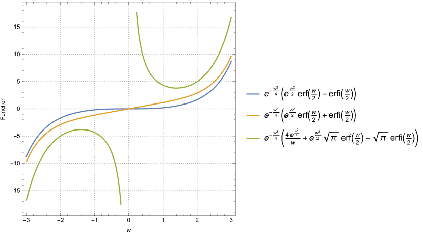
Figure 1: The qualitative behaviour of the three non-exponential terms of the closed-form solution (40) are presented. Blue line for the function $e^{-\frac{w^{2}}{4}}\left(e^{\frac{w^{2}}{2}}\text{{erf}}\left(\frac{w}{2}\right)-\text{{erfi}}\left(\frac{w}{2}\right)\right),$ orange line is for $e^{-\frac{w^{2}}{4}}\left(e^{\frac{w^{2}}{2}}\text{{erf}}\left(\frac{w}{2}\right)+\text{{erfi}}\left(\frac{w}{2}\right)\right)$ and green line is for the function $e^{-\frac{w^{2}}{4}}\left(\frac{4}{w}e^{\frac{w^{2}}{4}}+\sqrt{\pi}\left(e^{\frac{w^{2}}{2}}\text{{erf}}\left(\frac{w}{2}\right)-\text{{erfi}}\left(\frac{w}{2}\right)\right)\right)$

We apply the same procedure for the determination of similarity solutions for equation $\Phi_{B}$. We find similar reductions for the travel-wave solution, and for the scaling solutions. However we study the case where $\alpha+\beta=0$ for equation two which provides a new reduction.

4.3 Travel-wave solution for equation $\Phi_{B}$ and $\alpha+\beta=0$

For equation (2) with $\alpha+\beta=0$, we apply the Lie invariants of the symmetry vector $\left\{\Gamma_{2}+\gamma\Gamma_{3}+\delta\check{\Gamma}_{4}\right\}$, they are $u\left(t,x\right)=\delta t\left(x-\frac{\gamma}{2}t\right)+v\left(z\right)$,  $z=x-\gamma t$, while the reduced equation is

$$\gamma v^{\left(5\right)}-\left(\gamma\left(\gamma^{2}-1\right)+\alpha\delta z-\alpha v_{z}\right)v_{zzz}+\alpha\left(\gamma v_{zz}-\delta\right)v_{zz}=0,$$ (41)

Equation (41) can be integrated twice such that it becomes the third-order ordinary differential equation

$$\frac{\delta^{3}}{\gamma^{2}}v_{ZZZ}+\frac{\alpha\delta^{2}}{2\gamma}\left(v_{Z}\right)^{2}-\left(v_{0}+\alpha\delta Z\right)v_{Z}+\alpha\delta v+v_{0}\frac{v_{0}+\left(1-\gamma^{2}+\alpha Z\right)\delta}{\alpha\delta^{2}}+v_{1}=0.$$ (42)

where we have replaced $z=\frac{v_{0}+\left(1-\gamma^{2}+\alpha Z\right)\delta}{\alpha\delta^{2}}$.

Equation (42) admits the point symmetry $\partial_{Z}+\frac{\gamma}{\delta}t\partial_{w}$.  With the use of the later lie symmetry, equation (42) can be reduced further,

$$\delta^{5}\alpha Y_{XX}+\alpha^{2}\delta^{4}\gamma\sqrt{Y}-2v_{0}\alpha^{2}\gamma^{2}+\frac{2\gamma^{2}}{\sqrt{Y}}\left(\gamma v_{0}\left(v_{0}+1-\gamma^{2}\delta\right)+v_{1}\alpha\delta^{2}+\alpha^{2}\delta^{3}X\right)=0.$$ (43)

where the new variable are $\sqrt{Y}=\frac{\gamma}{\delta}Z-y_{Z}$ and $X=\frac{\gamma}{2\delta}W^{2}-y.$ The linearized equation (43) with the change of variables $Y\left(X\right)\rightarrow\sqrt{\varepsilon}Y\left(X\right)$ is described by the Aire functions.

5 Conclusion

In this work we studied by using Lie’s theory two fifth-order 1+1 partial differential equations which provide kink solutions. For these two equations we determine the admitted Lie points symmetries which for the two cases form a Lie algebra of dimension four, while when the free parameters of the equations have specific values the admitted Lie algebra has dimension six.

The one-dimensional optimal system is determined for all Lie algebras. We apply these results to reduce the differential equations and when it is feasible to write exact and analytic similarity solutions. We found that the kink solution which was found before [33] with the use of the Hirota’s method, can be constructed by using the Lie point symmetries.

The author in [33] proposed some families of 2+1 fifth-order partial differential equations as an extension of his results. The proposed equations which has kink solutions are

$$\Phi_{\Gamma}:u_{ttt}-u_{tyyyy}-u_{txx}-\alpha\left(u_{y}u_{ty}\right)_{y}=0,$$ (44)

$$\Phi_{\Delta}:u_{ttt}-u_{txxxx}-u_{tyyyy}-\alpha\left(u_{x}u_{tx}\right)_{x}=0,$$ (45)

while we introduce the 1+2 fifth-order partial differential equation

$$\Phi_{E}:u_{ttt}-u_{txxxx}-u_{tyyyy}-u_{txx}-u_{tyy}-\left(u_{x}u_{tx}\right)_{x}-\left(u_{y}u_{ty}\right)_{y}=0.$$ (46)

We apply the same analysis as before and we find that equation (44) admits the Lie point symmetries

$$\left\{\Gamma_{1},~{}\Gamma_{2},~{}\Gamma_{3},~{}\Gamma_{4}^{\prime}=\Gamma_{4}+\frac{1}{2}y\partial_{y},\Gamma_{5}=\partial_{y}\right\}$$ (47)

and the infinity number of symmetries $\Gamma_{\infty}=U\left(t,x\right)\partial_{u}$ where $U\left(t,x\right)$ is a solution of the partial differential equation $U_{ttt}-U_{txx}=0$.

Similarly, equation (44) is invariant under the one-parameter point transformations with generators the vector fields $\left\{\Gamma_{1},~{}\Gamma_{2},~{}\Gamma_{3},~{}\Gamma_{4}^{\prime},\Gamma_{5}\right\}$ while the infinity number of symmetries is $\Gamma_{\infty}=V\left(t,y\right)\partial_{u}$ with $V_{ttt}-V_{txx}=0$.

Finally, equation (46) admits the Lie point symmetries

$$\left\{\tilde{\Gamma}_{1},~{}~{}\tilde{\Gamma}_{2},~{}\tilde{\Gamma}_{3},~{}\tilde{\Gamma}_{4},\tilde{\Gamma}_{5},\tilde{\Gamma}_{6}^{{}^{\prime\prime}}=~{}\tilde{\Gamma}_{6}^{\prime}-y\partial_{y}+2y,\Gamma_{7}=\partial_{y}\right\}.$$ (48)

We observe that equations (44), (45) and (46) admit the Lie symmetries of (1), (2) extended in the two-dimensional flat space $\left\{x-y\right\}$. Hence, the above results are also applied and the similarity solutions hold but now in the plane $\left\{x-y\right\}$.

In a future work we plan to investigate the relation of conservation laws with the existence of kink solutions by using these equations as toy models.

References

• [1] S. Lie,Theorie der Transformationsgrupprn: Vol I, Chelsea, New York (1970)
• [2] S. Lie, Theorie der Transformationsgrupprn: Vol II, Chelsea, New York (1970)
• [3] S. Lie,Theorie der Transformationsgrupprn: Vol III, Chelsea, New York (1970)
• [4] E. Noether, Invariante Variationsprobleme Königlich Gesellschaft der Wissenschaften Göttingen Nachrichten Mathematik-physik Klasse 2, 235 (1918)
• [5] P.G.L. Leach, First integrals for the modified Emden equation $\ddot{q}+a\left(t\right)\dot{q}+q^{n}=0$, J. Math. Phys. 26, 510 (1985)
• [6] S. Moyo and P.G.L. Leach, A Note on the Integrability of a Class of Nonlinear Ordinary Differential Equations, J. Nonl. Math. Phys. 15, 159 (2008)
• [7] D.P. Mason and N. Roussos, Lie symmetry analysis and approximate solutions for non-linear radial oscillations of an incompressible Mooney–Rivlin cylindrical tube, J. Math. Anal. Appl. 245, 346 (2000)
• [8] A.A. Chesnokov, Symmetries and exact solutions of the shallow water equations for a two-dimensional shear flow, J. Appl. Mech. Techn. Phys. 49, 737 (2008)
• [9] M. Pandey, Lie Symmetries and Exact Solutions of Shallow Water Equations with Variable Bottom, Int. J. Nonl. Sci. Num. Sim. 16, 93 (2015)
• [10] S. Szatmari and A. Bihlo, Symmetry analysis of a system of modified shallow-water equations, Comm. Nonl. Sci. Num. Sim. 19, 530 (2014)
• [11] S. Jamal, A.H. Kara and A.K. Bokhari, Wave Equations in Bianchi Space-Times, Canadian J. Phys. 90, 667 (2012)
• [12] M. Tsamparlis and A. Paliathanasis, Lie and Noether symmetries of geodesic equations and collineations, Gen. Relativ. Grav. 42, 2957 (2010)
• [13] H. Azad and M.T. Mustafa, Symmetry analysis of wave equation on sphere, J. Math. Anal. Appl. 333, 1180 (2007)
• [14] A. Paliathanasis and M. Tsamparlis, Two dimensional dynamical systems which admit Lie and Noether symmetries, J. Phys. A: Math. Theor. 44, 175202 (2011)
• [15] A. Paliathanasis, M. Tsamparlis and M.T. Mustafa, Symmetry analysis of the Klein-Gordon equation in Bianchi I spacetimes, Comm. Non. Sci. Num. Sim. 55, 68 (2018)
• [16] A. Paliathanasis, One-Dimensional Optimal System for 2D Rotating Ideal Gas, Symmetry 11, 115 (2019)
• [17] K. S. Chou and C. Z. Qu, Optimal Systems and Group Classification of (1+2)-Dimensional Heat Equation, Acta Applicandae Mathematicae, 83, 257 (2004)
• [18] D. Huang and N.M. Ivanova, Group analysis and exact solutions of a class of variable coefficient nonlinear telegraph equations, J. Math. Phys., 48, 073507 (2007).
• [19] F.M. Mahomed. Symmetry group classification of ordinary differential equations, Math. Methods Appl. Sci. 30, 1995 (2007).
• [20] X. Xin, Y. Liu and X. Liu, Nonlocal symmetries, exact solutions and conservation laws of the coupled Hirota equations, Appl. Math. Lett. 55, 63 (2016)
• [21] S.V. Meleshko and V.P. Shapeev, Nonisentropic solutions of simple wave type of the gas dynamics equations, J. Nonl. Math. Phys. 18, 195 (2011)
• [22] G.M. Webb and G.P. Zank, Fluid relabelling symmetries, Lie point symmetries and the Lagrangian map in magnetohydrodynamics and gas dynamics, J. Math. Phys. A: Math. Theor. 40, 545 (2006)
• [23] S. Jamal and A.H. Kara, New higher-order conservation laws of some classes of wave and Gordon-type equations, Nonlinear Dynamics 67, 97 (2012)
• [24] A. Paliathanasis, Similarity inner solutions for the Pulsar equation, Math. Meth. Appl. Sci. 43, 716 (2020)
• [25] A. Paliathanasis, Lie symmetry analysis and one-dimensional optimal system for the generalized 2 + 1 Kadomtsev-Petviashvili equation, Phys. Scripta 95, 055223 (2020)
• [26] S. Jamal, Solutions of quasi-geostrophic turbulence in multi-layered configurations, Quaestiones Mathematicae 41, 409 (2018)
• [27] M.C. Nucci, Jacobi’s last multiplier, Lie symmetries, and hidden linearity: “Goldfishes” galore, Theor. Math. Phys. 151, 851 (2007)
• [28] J.F Carinena, J. de Lucas and M.F. Ranada, Jacobi multipliers, non-local symmetries, and nonlinear oscillators, J. Math. Phys. 56, 063505 (2015)
• [29] M.C. Nucci and P.G.L. Leach, Jacobi’s last multiplier and Lagrangians for multidimensional systems, J. Math. Phys. 49, 073517 (2008)
• [30] B. Muatjetjeja and C.M. Khalique, Benjamin–Bona–Mahony Equation with Variable Coefficients: Conservation Laws, Symmetry 6, 1026 (2014)
• [31] S. Jamal, Dynamical Systems: Approximate Lagrangians and Noether Symmetries, IJGMMP 16, 1950160 (2019)
• [32] T.-T. Zhang, On Lie symmetry analysis, conservation laws and solitary waves to a longitudinal wave motion equation, Appl. Math. Lett. 98, 199 (2019)
• [33] A.-M. Wazwaz, Kink solutions for three new fifth-order nonlinear equations, Appl. Math. Mod. 38, 110 (2014)
• [34] A.-M. Wazwaz, A new fifth order nonlinear integrable equation: multiple soliton solutions, Physica Scripta, Phys. Scr. 83, 015012 (2011)
• [35] A.-M. Wazwaz, A new fifth order nonlinear integrable equation: multiple soliton solutions, Phys. Scr. 83, 035003 (2011)
• [36] G. Wang, K. Yang, H. Gu, F. Guan and A.H. Kara, A (2+1)-dimensional sine-Gordon and sinh-Gordon equations with symmetries and kink wave solutions, Nucl. Phys. B 953, 114956 (2020)
• [37] M. Kumar, D.V. Tanwar and R. Kumar, On Lie symmetries and soliton solutions of (2+1)-dimensional Bogoyavlenskii equations, Nonlinear Dynamics, 94, 2547 (2018)
• [38] A. Bansal, A. Biswas, A.S. Alshomrani, M. Ekici, Q. Zhou and M.R. Belic, Optical solitons with nonlocal-parabolic combo nonlinearity by Lie symmetry analysis coupled with modified G’/G-expansion, Results in Physics 15, 102713 (2019)
• [39] A.-M. Wazwaz and L. Kaur, Complex simplified Hirota’s forms and Lie symmetry analysis for multiple real and complex soliton solutions of the modified KdV–Sine-Gordon equation, Nonlinear Dynamics 95, 2209 (2019)
• [40] M. Kumar and A.K. Tiwari, Some more solutions of Kadomtsev–Petviashvili equation, Comp. Math. Appl. 75, 1434 (2018)
• [41] C.M. Khalique and A. Biswas, 1-Soliton Solution of the Nonlinear Schrödinger’s Equation with Kerr Law Nonlinearity Using Lie Symmetry Analysis, Int. J. Theor. Phys. 48, 1872 (2009)
• [42] M. Ruggieri, Kink Solutions for a Class of Generalized Dissipative Equations, Abstract and Applied Analysis 2012, 237135 (2012)
• [43] N.H. Ibragimov, CRC Handbook of Lie Group Analysis of Differential Equations, Volume I: Symmetries, Exact Solutions, and Conservation Laws, CRS Press LLC, Florida (2000)
• [44] G.W. Bluman and S. Kumei, Symmetries of Differential Equations, Springer-Verlag, New York, (1989)
• [45] H. Stephani, Differential Equations: Their Solutions Using Symmetry, Cambridge University Press, New York, (1989)
• [46] P.J. Olver, Applications of Lie Groups to Differential Equations, Springer-Verlag, New York, (1993)
• [47] M.J. Ablowitz, A. Ramani and H. Segur,  Nonlinear evolution equations and ordinary differential equations of painlevè type, Lettere al Nuovo Cimento 23, 333 (1978)
• [48] M.J. Ablowitz, A. Ramani and H. Segur, A connection between nonlinear evolution equations and ordinary differential equations of P-type. I, J. Math. Phys. 21, 715 (1980)
• [49] M.J. Ablowitz, A. Ramani and H. Segur, A connection between nonlinear evolution equations and ordinary differential equations of P-type. II, J. Math. Phys. 21, 1006 (1980)
• [50] A. Ramani, B. Grammaticos and T. Bountis, The Painlevé property and singularity analysis of integrable and non-integrable systems, Phys. Rept. 180, 159 (1989)
• [51] A. Paliathanasis and P.G.L. Leach, Nonlinear Ordinary Differential Equations: A discussion on Symmetries and Singularities, IJGMMP 13, 1630009 (2016)
• [52] A.K. Halder, A. Paliathanasis and P.G.L. Leach, Singularity analysis of a variant of the Painlevé–Ince equation, Appl. Math. Lett. 98, 70 (2019)