Analysis of coherence in turbulent stratified wakes using spectral proper orthogonal decomposition

Abstract

We use spectral proper orthogonal decomposition (SPOD) to extract and analyze coherent structures in the turbulent wake of a disk at Reynolds number $\Rey=5\times 10^{4}$ and Froude numbers Fr = $2,10$. We find that the SPOD eigenspectra of both wakes exhibit a low-rank behavior and the relative contribution of low-rank modes to total fluctuation energy increases with $x/D$. The vortex shedding (VS) mechanism, which corresponds to $\mbox{{St}}\approx 0.11-0.13$ in both wakes, is active and dominant throughout the domain in both wakes. The continual downstream decay of the SPOD eigenspectrum peak at the VS mode, which is a prominent feature of the unstratified wake, is inhibited by buoyancy, particularly for $\mbox{{Fr}}=2$. The energy at and near the VS frequency is found to appear in the outer region of the wake when the downstream distance exceeds $Nt=Nx/U=6-8$. Visualizations show that unsteady internal gravity waves (IGWs) emerge at the same $Nt=6-8$. A causal link between the VS mechanism and the unsteady IGW generation is also established using the SPOD-based reconstruction and analysis of the pressure-transport term. These IGWs are also picked up in SPOD analysis as a structural change in the shape of the leading SPOD eigenmode. The $\mbox{{Fr}}=2$ wake shows layering in the wake core at $Nt>15$ which is captured by the leading SPOD eigenmodes of the VS frequency at downstream locations $x/D>30$. The VS mode of the $\mbox{{Fr}}=2$ wake is streamwise-coherent, consisting of V-shaped structures at $x/D\gtrsim 30$. Overall, we find that the coherence of wakes, initiated by the VS mode at the body, is prolonged by buoyancy to far downstream. Also, this coherence is spatially modified by buoyancy into horizontal layers and IGWs. Low-order truncations of SPOD modes are shown to efficiently reconstruct important second-order statistics.

[figure]subcapbesideposition=top [subfigure]subcapbesideposition=top

1 Introduction

Turbulent wakes are ubiquitous both in nature and man-made devices. From flow past moving vehicles (Grandemange et al., 2015) to flow past topographic features (Puthan et al., 2021) in oceans, they play an important role in transporting momentum and energy across large distances from the wake generator. In the ocean and the atmosphere, the background density often has a stable density stratification. Buoyancy in a stable background enables the emergence of several distinctive features, e.g., suppression of vertical turbulent motions (Spedding, 2002b), multistage wake decay (Lin & Pao, 1979; Spedding, 1997), appearance of coherent structures in the late wake (Lin & Pao, 1979; Lin et al., 1992a), and formation of steady (Hunt & Snyder, 1980) and unsteady (Gilreath & Brandt, 1985; Bonneton et al., 1993) internal gravity waves, to name a few. A majority of wake studies utilize axisymmetric body shapes (sphere, disk, spheroid, etc.) since such canonical shapes make it convenient to understand the phenomenology of turbulent stratified wakes.

The existence of coherent structures has been established to be an universal feature of both unstratified and stratified turbulent wakes. The Kárman vortex street associated with vortex shedding from the body at a specific frequency is a well known feature of unstratified bluff body wakes which arises from the global instability of the $m=1$ azimuthal mode as was demonstrated for a sphere by Natarajan & Acrivos (1993) and Tomboulides & Orszag (2000). The Strouhal number (St) associated with vortex shedding varies with the shape of the body. Vortex shedding has been investigated in stratified wakes too. Lin et al. (1992b) conducted a detailed experimental investigation of stratified flow past a sphere of diameter $D$ towed with speed $U$ in a fluid with buoyancy frequency $N$ for $5\leq\Rey\ (UD/\nu)\leq 10^{4}$ and $0.005\leq\mbox{{Fr}}\ (U/ND)\leq 20$. At $\mbox{{Fr}}\gtrsim 2$, they found that St in the near wake of the sphere, at $x/D\approx 3$, attained a constant value of $\mbox{{St}}\approx 0.18$, same as in the unstratified wake. For $\mbox{{Fr}}\lesssim 2$, the vortex shedding was two-dimensional and St increased with decreasing Fr in the near wake, similar to the trend in the flow past a circular cylinder. Chomaz et al. (1993) identified four regimes, differentiated by the value of Fr, in the near wake of a sphere. These regimes showed structural differences in the shed vortices and their interactions with the lee wave field.

Another distinctive feature of the stratified wakes is the generation of IGWs which are of two types: (i) body generated steady lee waves and (ii) wake generated unsteady IGWs. In their pioneering work on the wake of a self-propelled slender body, Gilreath & Brandt (1985) noted a coupling between the unsteady IGWs in the outer wake and the wake core turbulence, which suggests that the generation of the unsteady IGWs is inherently nonlinear in nature. Bonneton et al. (1993) and Bonneton et al. (1996) examined IGWs in the flow past a sphere. Lee waves were found to dominate when $\mbox{{Fr}}\lesssim 0.75$ and, for $\mbox{{Fr}}\gtrsim 2.25$, the downstream wake was dominated by the unsteady IGWs. Analysis of the density and velocity spectra in the outer wake showed a distinct peak at the vortex shedding frequency of sphere, $\mbox{{St}}\approx 0.18$. Brandt & Rottier (2015) found wake turbulence to be a dominant source term for IGWs at $\mbox{{Fr}}\gtrsim 1$ in their experimental work on sphere wakes. However, they did not expand on the spectral characteristics of these wake-generated IGWs. Recently, Meunier et al. (2018) also conducted a theoretical and experimental study of waves generated by various wake generators, focusing primarily on the scalings of wavelengths and amplitudes across various Fr and wake generators. Various aspects of IGWs have also been studied through numerical simulations (Abdilghanie & Diamessis, 2013; Zhou & Diamessis, 2016; Ortiz-Tarin et al., 2019; Rowe et al., 2020).

In the last two decades, the rise in computing power has enabled a number of numerical studies which have improved our understanding of stratified wakes. A large body of numerical literature employs the temporal model wherein the wake generator is not included (Gourlay et al., 2001; Dommermuth et al., 2002; Brucker & Sarkar, 2010; Diamessis et al., 2011; de Stadler & Sarkar, 2012; Abdilghanie & Diamessis, 2013; Redford et al., 2015; Zhou & Diamessis, 2019; Rowe et al., 2020). Instead, these simulations are initialized with synthetic mean and turbulence profiles mimicking those of a wake. Body-inclusive simulations which resolve the flow at the wake generator and at a high enough $\Rey$ that sustain turbulence are relatively recent (Orr et al., 2015; Pal et al., 2016, 2017; Ortiz-Tarin et al., 2019; Chongsiripinyo & Sarkar, 2020).

The database from the body-inclusive simulation of Chongsiripinyo & Sarkar (2020), hereafter referred to as CS2020, will be interrogated in this paper to analyze spatio-temporal coherence. CS2020 perform large eddy simulation (LES) of flow past a disk at $\Rey=5\times 10^{4}$ and at various values of Fr. The authors find that the wake transitions through three different regimes of stratified turbulence (provided buoyancy Reynolds number $>O(1)$), each with distinctive turbulence properties: weakly stratified turbulence (WST) which commences when the turbulent Froude number $Fr_{h}$ decreases to $O(1)$, intermediately stratified turbulence (IST) when $Fr_{h}$ decreases to $O(0.1)$, and strongly stratified turbulence (SST) when $Fr_{h}$ reduces to to $O(0.01)$. Here $\mbox{{Fr}}_{h}=u_{h}^{\prime}/Nl_{v}$, where $u^{\prime}_{h}$, $N$, and $l_{v}$ are r.m.s. horizontal velocity fluctuations, buoyancy frequency, and a characteristic turbulent vertical lengthscale, respectively. In the WST regime, the turbulence is not yet appreciably affected by buoyancy effects. Anisotropy in turbulent velocity components, which is a key manifestation of stratification, has not kicked in yet (see figure 8 of CS2020). As the flow evolves downstream, turbulence anisotropy keeps increasing and the turbulence transitions to the IST regime at $\mbox{{Fr}}_{h}\sim O(0.1)$. The SST regime, which commences at $\mbox{{Fr}}_{h}\approx 0.03$, is characterized by a strong anisotropy in turbulence. An indication of arrival of this regime is the scaling of the vertical lengthscale with $u^{\prime}_{h}/N$ as derived by Billant & Chomaz (2001) (also see figure 12 in CS2020). In the SST regime, mean defect velocity and $u^{\prime}_{h}$ decay at the same rate of $x^{-0.18}$ while vertical turbulent velocity ($u^{\prime}_{z}$) decays at a faster rate of $x^{-1}$. Regime classification based on turbulence instead of mean velocity was introduced in the context of stratified homogeneous turbulence, e.g., Brethouwer et al. (2007), and was recently extended to stratified turbulent wakes by Zhou & Diamessis (2019) and CS2020.

With the huge amount of numerical and experimental data becoming available, data-driven modal decomposition techniques have also seen an unprecedented rise in their use to understand the dynamics and role of coherent structures in turbulent flows. These techniques have also been used to construct reduced-order models of these flows. One popular technique is proper orthogonal decomposition (POD), proposed by Lumley (1967, 1970) in the context of turbulent flows, which provides a set of modes ordered hierarchically in terms of energy content. Another popular technique is dynamic mode decomposition (DMD), described by Schmid (2010), which decomposes the flow into a set of spatial modes, each oscillating at a specific frequency.

However, applications of modal decomposition to stratified flows are few in number. Diamessis et al. (2010) performed snapshot POD (Sirovich (1987)) on the vorticity field from a temporal simulation at $\Rey=5\times 10^{3}$ and $\mbox{{Fr}}=2$, noting a link between wake core structures and the angle of emission of IGWs in the outer wake. The layered wake core structure, which is a distinctive feature of stratified turbulent wakes, was found in the POD modes with lower modal index (corresponding to higher energy). As the modal index increased, the wake core was found to be dominated by small-scale incoherent turbulence. Xiang et al. (2017) performed spatial and temporal DMD on the experimental data of the stratified wake of a grid showing that DMD modes successfully captured lee waves and Kelvin-Helmholtz (KH) instability in the near wake ($Nt<10$). Nidhan et al. (2019) performed three-dimensional (3D) and planar two-dimensional (2D) DMD on the sphere wake at $\Rey=500$ and $10^{4}$, respectively. At $\Rey=500$ and $\mbox{{Fr}}=0.125$, they found that the 2D vortex shedding in the center-horizontal plane and ‘surfboard’ structures in the center-vertical plane corresponded to the same DMD mode oscillating at the vortex shedding frequency of $\mbox{{St}}\approx 0.19$. At the higher $\Rey=10^{4}$, DMD modes associated with vortex shedding showed IGWs in the outer wake.

In the present work, we use spectral proper orthogonal decomposition (SPOD), originally proposed by Lumley (1967, 1970) and recently revisited by Towne et al. (2018), to identify and analyze the coherent structures in the turbulent stratified wake of a disk at $\Rey=5\times 10^{4}$. In its original form, POD is prohibitively expensive to apply on today’s large numerical databases with high space-time resolution. The form put forward by Towne et al. (2018) leverages the temporal symmetry of statistically stationary flows to improve computational tractability. SPOD decomposes statistically stationary flows into energy-ranked modes with monochromatic frequency content, thus separating both the temporal and spatial scales in the flow, unlike the popular snapshot variant given by Sirovich (1987). SPOD has been used extensively in recent times for analysis of coherent structures and reduced-order modeling in a variety of unstratified flow configurations: (i) turbulent jets (Semeraro et al., 2016; Schmidt et al., 2017, 2018; Nogueira et al., 2019; Nekkanti & Schmidt, 2020b), (ii) turbulent wakes (Nidhan et al., 2020), (iii) channel (Muralidhar et al., 2019) and pipe (Abreu et al., 2020) flows, (iv) flow reconstruction (Nekkanti & Schmidt, 2020a) and low-order modeling (Chu & Schmidt, 2021), (v) wakes of actuator disks in turbulent environments (Ghate et al., 2018, 2020), etc.

The formation of coherent pancake vortices in the Q2D late wake does not necessarily require vortex shedding from the body as was demonstrated by Gourlay et al. (2001) whose temporally evolving model at $\mbox{{Fr}}=10$ did not include the vortex shedding mode but still exhibited Q2D-regime pancake vortices. Our interest is also in coherent structures but in a region of the far wake which is at large $x/D$ but still not in the Q2D regime. We ask how does buoyancy affect the space-time coherence as the flow progresses from the near wake to the far wake? What are the salient differences between the unstratified ($\mbox{{Fr}}=\infty$) and stratified wakes in the context of coherent structures? We will address these questions by analyzing the LES dataset of CS2020, specifically the wakes at $\mbox{{Fr}}=2$ and 10. We adopt SPOD for the data analysis since it is well suited to extract modes which have spatial and temporal coherence and thus track the evolution of specific modes, e.g. the vortex shedding (VS) mode, as the wake evolves downstream. The SPOD analysis also allows us to address a second set of questions: (i) are coherent modes linked to unsteady IGWs and (ii) how is the energy in dominant coherent structures distributed across the wake cross-section during downstream evolution? SPOD modes can also be useful for constructing reduced-order models prompting the third question: what is the efficacy of different SPOD modal truncations in regard to the reconstruction of various second-order turbulence statistics in turbulent stratified wakes?

The rest of the paper is organized as follows. §2 and §3 give a brief overview of the numerical methodology and SPOD technique. Visualizations of $\mbox{{Fr}}=2$ and $10$ wakes are presented in §4. The characteristics of SPOD eigenvalues and eigenspectrum are discussed in §5. The VS mode and its link to the unsteady IGWs are discussed in detail in §6. Sections §7 and §8 discuss the spatial structure of SPOD eigenmodes and trends in the reconstruction of second-order statistics by sets of truncated SPOD modes, respectively. Finally, the discussion and conclusions are presented in §9.

2 Numerical methodology

We use the numerical database of the wake of a circular disk at $\Rey$ = $5\times 10^{4}$ from CS2020. In particular, we analyze the datasets of stratified wakes at $\mbox{{Fr}}=2$ and $10$ from their numerical database. CS2020 use high-resolution large eddy simulation (LES) to numerically solve the filtered Navier-Stokes equations system along with density diffusion equation under the Boussinesq approximation.

These equations are as follows:

continuity,

$$\frac{\partial u_{i}}{\partial x_{i}}=0,$$ (1)

momentum,

$$\frac{\partial u_{i}}{\partial t}+\frac{\partial(u_{i}u_{j})}{\partial x_{j}}=-\frac{\partial p}{\partial x_{i}}+\frac{1}{\Rey}\frac{\partial}{\partial x_{j}}\Big{[}\Big{(}1+\frac{\nu_{s}}{\nu}\Big{)}\frac{\partial u_{i}}{\partial x_{j}}\Big{]}-\frac{1}{\mbox{{Fr}}^{2}}\rho^{\prime}\delta_{i3},$$ (2)

and density diffusion,

$$\frac{\partial\rho}{\partial t}+\frac{\partial(\rho u_{j})}{\partial x_{j}}=\frac{1}{\Rey\Pran}\frac{\partial}{\partial x_{j}}\Big{[}\Big{(}1+\frac{\kappa_{s}}{\kappa}\Big{)}\frac{\partial\rho}{\partial x_{j}}\Big{]},$$ (3)

where $u_{i}$ corresponding to $i=1,2,$ and $3$ refer to velocity in the streamwise ($x_{1}$ or $x$), lateral ($x_{2}$ or $y$), and vertical ($x_{3}$ or $z$) directions, respectively. Gravity acts in the vertical direction (2). The density field is decomposed into a background profile, $\rho_{b}(z)=\rho_{o}+(\mathop{}\!\mathrm{d}\rho_{b}/\mathop{}\!\mathrm{d}z)z$ (where $K$ is a constant), and density deviation ($\rho^{\prime}$). Thus $\rho(x,y,z,t)=\rho_{b}(z)+\rho^{\prime}(x,y,z,t)$. In (2), $\nu_{s}$ and $\nu$ refer to the subgrid kinematic viscosity obtained from LES and kinematic viscosity of the fluid, respectively. Likewise, $\kappa_{s}$ and $\kappa$ in equation (3) refer to the subgrid density diffusivity and density diffusivity of the fluid, respectively.

(1) - (3) are non-dimensionalized using the following parameters: (i) free stream velocity ($U_{\infty}$) for velocity field, (ii) diameter of disk ($D$) for spatial locations $x_{i}$, (iii) dynamic pressure ($\rho_{o}U_{\infty}^{2}$) for pressure field, (iv) advection timescale ($D/U_{\infty}$) for time $t$, and (iv) $-(\mathop{}\!\mathrm{d}\rho_{b}/\mathop{}\!\mathrm{d}z)D$ for density deviation. There are three non-dimensional parameters of interest: (1) body-based Reynolds number ($\Rey$) defined as $U_{\infty}D/\nu$, (2) body-based Froude number (Fr) defined as $U_{\infty}/ND$ where $N$ is the buoyancy frequency, $N^{2}=-g/\rho_{o}(\mathop{}\!\mathrm{d}\rho_{b}/\mathop{}\!\mathrm{d}z)$, and (3) Prandtl number ($\Pran$) defined as $\nu/\kappa$ which is set as 1 in CS2020 simulations. $\kappa_{s}$ is also set equal to $\nu_{s}$ for the LES simulations.

A cylindrical coordinate system is adopted and the disk is represented using the immersed boundary method (IBM) of Balaras (2004); Yang & Balaras (2006). Spatial derivatives are computed using second-order central finite differences and temporal marching is performed using a fractional step method which combines a low-storage Runge-Kutta scheme (RKW3) with the second-order Crank-Nicolson scheme. The kinematic subgrid viscosity ($\nu_{s}$) and density diffusivity ($\kappa_{s}$) are obtained using the dynamic eddy viscosity model of Germano et al. (1991). At the inlet and outlet, Dirichlet inflow and Orlanski-type convective (Orlanski (1976)) boundary conditions are specified, respectively. The Neumann boundary condition is used at the radial boundary for the density and velocity fields. To prevent the spurious propagation of internal waves upon reflection from the boundaries, sponge regions with Rayleigh-damping are employed at radial, inlet, and outlet boundaries.

The radial and streamwise domains span $0\leq r/D\leq 80$ and $-30\leq x/D\leq 125$, respectively. A large radial extent facilitates weakening of the IGWs before they hit the boundary and thereby also controls the amplitude of spurious reflected waves. The distribution of grid points are as follows: $N_{r}=531$ in the radial direction, $N_{\theta}=256$ in the azimuthal direction, and $N_{x}=4608$ in the streamwise direction, resulting in approximately 530 million elements. The grid resolution is excellent by LES standards in all three directions. Readers may refer to Chongsiripinyo & Sarkar (2020) for more details on the grid resolution and numerical scheme.

3 Spectral proper orthogonal decomposition - theory and present application

In this work, we employ spectral POD (SPOD) to study the dynamics of coherent structures in stratified wakes, rather than the more commonly employed snapshot POD (Sirovich, 1987). SPOD enables the identification of dominant structures evolving coherently in both space and time by exploiting temporal correlation among flow snapshots. This approach is particularly well-suited for flow configurations like turbulent wakes which are known to be dominated by mechanisms operating at specific frequencies, e.g., vortex shedding, pumping of recirculation bubble, shear layer breakdown, to name a few (Berger et al., 1990). On the contrary, snapshot POD assumes each snapshot of the flow to be an independent realization. As a result, the temporal coherence of POD modes is not guaranteed. Furthermore, it can be also shown that the coefficients dictating the temporal evolution of snapshot POD modes are broadband, i.e., containing contributions from a range of frequencies (Towne et al., 2018). SPOD requires a larger amount of time-resolved data compared to snapshot POD. Hence, snapshot POD has dominated the literature compared to SPOD.

3.1 Theory of SPOD for statistically-stationary stratified flows

For the SPOD analysis of stratified wakes, the fluctuating density fields $(\rho^{\prime}(\mathbf{x},t))$ and velocity fields $(\mathbf{u}^{\prime}(\mathbf{x},t)=[{u}_{r}^{\prime}(\mathbf{x},t),{u}_{\theta}^{\prime}(\mathbf{x},t),{u}_{x}^{\prime}(\mathbf{x},t)]^{T})$ are taken together as a single state-space field $\boldsymbol{\Lambda}(\textbf{x},t)=[\mathbf{u}^{\prime}(\mathbf{x},t),\rho^{\prime}(\mathbf{x},t)]^{T}$. Following Lumley (1970), we seek POD modes $\boldsymbol{\Psi}(\mathbf{x},t)$ that have maximum ensembled-average projection on $\boldsymbol{\Lambda}(\mathbf{x},t)$, expressed as:

$$\max_{\boldsymbol{\Psi}}\frac{\langle|\{\boldsymbol{\Lambda}(\mathbf{x},t),\boldsymbol{\Psi}(\mathbf{x},t)\}|^{2}\rangle}{\{\boldsymbol{\Psi}(\mathbf{x},t),\boldsymbol{\Psi}(\mathbf{x},t)\}},$$ (4)

where $\langle.\rangle$ denotes the ensemble average. We define the inner product $\{\boldsymbol{\Lambda}^{(1)}(\mathbf{x},t),\boldsymbol{\Lambda}^{(2)}(\mathbf{x},t)\}$ as:

$$\{\boldsymbol{\Lambda^{(1)}}(\mathbf{x},t),\boldsymbol{\Lambda^{(2)}}(\mathbf{x},t)\}=\int_{-\infty}^{\infty}\int_{\Omega}\boldsymbol{\Lambda^{(2)}}^{*}(\mathbf{x},t)\mathop{}\!\mathrm{diag}\Big{(}1,1,1,\frac{g^{2}}{\rho^{2}_{o}N^{2}}\Big{)}\boldsymbol{\Lambda^{(1)}}(\mathbf{x},t)\mathop{}\!\mathrm{d}\mathbf{x}\mathop{}\!\mathrm{d}t,$$ (5)

where $(.)^{*}$ denotes the Hermitian transpose. The so-defined inner-product norm ensures that the obtained POD modes are optimal in terms of capturing two-times the overall sum of turbulent kinetic energy (TKE) and turbulent potential energy (TPE), where TKE $=\langle u^{\prime}_{i}u^{\prime}_{i}\rangle/2$ and TPE=$\frac{g^{2}}{2\rho^{2}_{o}N^{2}}\langle\rho^{\prime}\rho^{\prime}\rangle$.

Following Holmes et al. (2012), (4) can be expressed as a Fredholm-type integral eigenvalue problem as follows:

$$\int_{-\infty}^{\infty}\int_{\Omega}R_{ij}(\mathbf{x},\mathbf{x}^{\prime},t,t^{\prime})\mathbf{W}(\mathbf{x}^{\prime})\Psi^{(n)}_{j}(\mathbf{x}^{\prime},t^{\prime})\mathop{}\!\mathrm{d}\mathbf{x}^{\prime}\mathop{}\!\mathrm{d}t^{\prime}=\lambda^{(n)}\Psi^{(n)}_{i}(\mathbf{x},t),$$ (6)

where $\mathbf{W}(\mathbf{x})$ is a positive-definite Hermitian matrix accounting for the weights of each variable as defined in the (5). In (6), $\lambda^{(n)}$ and $\Psi^{(n)}_{i}(\mathbf{x},t)$ correspond to the $n^{th}$ eigenvalue and the $i^{th}$ component of the $n^{th}$ eigenmode. The kernel $R_{ij}(\mathbf{x},\mathbf{x}^{\prime},t,t^{\prime})$ which is the two-point two-time correlation tensor, is defined as follows:

$$R_{ij}(\mathbf{x},\mathbf{x}^{\prime},t,t^{\prime})=\langle u^{\prime}_{i}(\mathbf{x},t)u^{\prime}_{j}(\mathbf{x}^{\prime},t^{\prime})\rangle,\ \ \ \ i,j=1,2,3,$$ (7)

$$R_{i4}(\mathbf{x},\mathbf{x}^{\prime},t,t^{\prime})=\langle u^{\prime}_{i}(\mathbf{x},t)\rho^{\prime}(\mathbf{x}^{\prime},t^{\prime})\rangle,\ \ \ \ i=1,2,3,$$ (8)

$$R_{4j}(\mathbf{x},\mathbf{x}^{\prime},t,t^{\prime})=\langle\rho^{\prime}(\mathbf{x},t)u^{\prime}_{j}(\mathbf{x}^{\prime},t^{\prime})\rangle,\ \ \ \ j=1,2,3,$$ (9)

$$R_{44}(\mathbf{x},\mathbf{x}^{\prime},t,t^{\prime})=\langle\rho^{\prime}(\mathbf{x},t)\rho^{\prime}(\mathbf{x}^{\prime},t^{\prime})\rangle.\ \ \ \$$ (10)

For statistically stationary flows, such as the turbulent stratified wake in the present case, the kernel $R_{ij}(\mathbf{x},\mathbf{x}^{\prime},t,t^{\prime})$ is only a function of time difference $\tau=t-t^{\prime}$, $\mathbf{x}$, and $\mathbf{x}^{\prime}$. Furthermore, it can be Fourier-transformed in the temporal direction as follows:

$$R_{ij}(\mathbf{x},\mathbf{x}^{\prime},\tau)=\int_{-\infty}^{\infty}S_{ij}(\mathbf{x},\mathbf{x^{\prime}},f)e^{i2\pi f\tau}\mathop{}\!\mathrm{d}f,$$ (11)

where $S_{ij}(\mathbf{x},\mathbf{x}^{\prime},f)$ is the Fourier transform of the kernel $R_{ij}(\mathbf{x},\mathbf{x}^{\prime},\tau)$. Using (11), the Fredholm-type eigenvalue problem in (6) can be transformed into an equivalent eigenvalue problem which is solved at each frequency $f$, following Towne et al. (2018),

$$\int_{\Omega}S_{ij}(\mathbf{x},\mathbf{x}^{\prime},f)\mathbf{W}(\mathbf{x}^{\prime})\Phi^{(n)}_{j}(\mathbf{x}^{\prime},f)\mathop{}\!\mathrm{d}\mathbf{x}^{\prime}=\lambda^{(n)}(f)\,\Phi^{(n)}_{i}(\mathbf{x},f),$$ (12)

where $\lambda^{(n)}(f)$ are the eigenvalues at $f$ and $\Phi^{(n)}_{i}(\mathbf{x},f)=\Psi^{(n)}_{i}(\mathbf{x},t)e^{-i2\pi ft}$ are the modified eigenmodes. The eigenvalues are ordered such that $\lambda^{(1)}(f)\geq\lambda^{(2)}(f)\geq.\ .\ .\ \geq\lambda^{(n)}(f)$. The sum over all the eigenvalues at frequency $f$ equates to two-times the total fluctuation energy content, i.e., $\langle u^{\prime}_{i}u^{\prime}_{i}\rangle$ $+$ $\frac{g^{2}}{\rho^{2}_{o}N^{2}}\langle\rho^{\prime}\rho^{\prime}\rangle$ at that frequency. The obtained eigenmodes in the frequency space are spatially orthogonal to each other such that:

$$\int_{\Omega}\boldsymbol{\Phi}^{*(n)}(\mathbf{x},f)\mathbf{W}(\mathbf{x})\boldsymbol{\Phi}^{(m)}(\mathbf{x},f)\mathop{}\!\mathrm{d}\mathbf{x}=\delta_{mn},$$ (13)

where $\delta_{mn}$ is the Dirac-delta function.

3.2 Numerical implementation of SPOD for current work

In this work, we primarily present results from SPOD on two-dimensional planes at various $x/D$ $-$ ranging from $x/D=10$ to $100$ $-$ sampled at a spacing of approximately $5D$. The domain of $10\leq x/D\leq 100$ spans: (i) $5\leq Nt_{2}\leq 50$ for $\mbox{{Fr}}=2$ and (ii) $1\leq Nt_{10}\leq 10$ for $\mbox{{Fr}}=10$ in terms of buoyancy time. In the radial direction, the SPOD domain spans $0\leq r/D\leq 10$, resulting in a total of $N^{SPOD}_{r}=333$ points. In the azimuthal direction, the number of grid points $N_{\theta}=256$.

For numerical implementation, the mean-subtracted data, consisting of $N$ temporal snapshots, is divided into $N_{blk}$ blocks with an overlap of $N_{ovlp}$ snapshots. Each block contains $N_{freq}$ entries: $\mathbf{Q}=[\mathbf{q}^{(1)},\mathbf{q}^{(2)},\mathbf{q}^{(3)},\cdots\mathbf{q}^{(N_{freq})}]$. Here, $\mathbf{q}^{(i)}=[\mathbf{u^{\prime}}^{(i)},\rho^{\prime(i)}]^{T}$ where $\mathbf{u^{\prime}}$ and $\rho^{\prime}$ are velocity and density fluctuations, respectively. Thereafter, discrete Fourier transform (DFT) of each block is performed in the temporal direction and the ensemble of $N_{blk}$ Fourier realizations of any given frequency, let us say $f$, is collected as $\mathbf{\hat{Q}}_{f}=[\mathbf{q}^{(1)(f)},\mathbf{q}^{(2)(f)},\mathbf{q}^{(3)(f)},\cdots\mathbf{q}^{(N_{blk})(f)}]$. Once, $\mathbf{\hat{Q}}_{f}$ is obtained, SPOD eigenvalues and eigenvectors corresponding to $f$ are given by the following eigenvalue decomposition:

$$\hat{\mathbf{Q}}^{*}_{f}\mathbf{W}\hat{\mathbf{Q}}_{f}\boldsymbol{\Gamma}_{f}=\boldsymbol{\Gamma}_{f}\boldsymbol{\Lambda}_{f},$$ (14)

where $\boldsymbol{\Lambda}_{f}=diag\Big{(}\lambda^{(1)}_{f},\lambda^{(1)}_{f},\cdots\lambda^{(N_{blk})}_{f}\Big{)}$ is a diagonal matrix containing eigenvalues ranked in the decreasing order of energy content from $i=1$ to $N_{blk}$. The corresponding spatial eigenmodes $\hat{\boldsymbol{\Phi}}_{f}$ can be obtained as $\hat{\boldsymbol{\Phi}}_{f}=\hat{\mathbf{Q}}_{f}\boldsymbol{\Gamma}_{f}\boldsymbol{\Lambda}_{f}^{-1/2}$. In (14), $\mathbf{W}$ is a diagonal matrix of size $4N^{SPOD}_{r}N_{\theta}$, containing the numerical quadrature weights multiplied by coefficients required to form the energy quantities given in (5).

The parameters for SPOD are set as follows: (i) total number of snapshots $N=7168$ with consecutive snapshots separated by $\Delta tD/U_{\infty}\approx 0.09$ and $0.104$ for $\mbox{{Fr}}=2$ and $10$, respectively, (ii) number of frequencies $N_{freq}=512$, and (iii) overlap between blocks $N_{ovlp}=256$, resulting in total of $N_{blk}=\frac{N-N_{ovlp}}{N_{freq}-N_{ovlp}}=27$ SPOD modes at each frequency. Interested readers are referred to Towne et al. (2018) and Schmidt & Colonius (2020) for more details on the theoretical aspects and numerical implementation of SPOD.

Most of the results are obtained from SPOD analyses at constant $x/D$ planes with modes maximizing the two-times sum of TKE and TPE. However, for some results, we perform additional SPOD analyses. For example, to illustrate the streamwise variation of a certain leading-order SPOD mode in §7, we perform SPOD analysis on fluctuating velocity and density fields at the center-vertical plane ($y=0$ plane) with reduced number of snapshots $N=5376$ and half-resolution in vertical and streamwise directions. $N_{freq}$ and $N_{ovlp}$ are kept the same as SPOD on fixed $x/D$ planes. The spatial resolution and $N$ are reduced to avoid memory limitations since large matrices with complex double precision have to be stored in the intermediate steps of SPOD. Also in §6, we present results from SPOD analyses of the $\mbox{{Fr}}=2$ wake (at constant $x/D$ planes) with (i) density fluctuations replaced by pressure fluctuations and (ii) norm defined such as to maximize the sum of $\langle p^{\prime}p^{\prime}\rangle$ and $\langle u^{\prime}_{i}u^{\prime}_{i}\rangle$. $N,N_{freq}$, and $N_{blk}$ are kept the same as in the previous paragraph. The motivation behind performing this additional set of SPOD analyses is explained in §6.

4 Flow visualizations

Three-dimensional visualizations of the $Q$ criterion and planar views of the vorticity and velocity fields in this section provide a first look at the vortical and unsteady IGW structure of the simulated wakes. The structure of the steady (in a frame attached to the disk) lee wave field is not discussed in this paper.

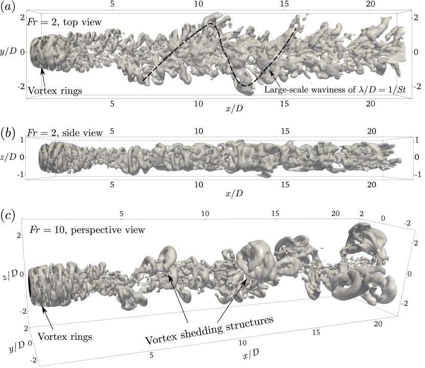
Figure 1: Isosurfaces of instantaneous $Q$ criterion at $Q=0.01$: (a,b) $\mbox{{Fr}}=2$ and (c) $\mbox{{Fr}}=10$. Streamwise domain is limited to $0<x/D<20$ for clarity.

To emphasize the large-scale coherent structures, the instantaneous velocity fields have been filtered using a SciPy Gaussian low-pass filter (gaussian_filter) in all three directions with standard deviation $\sigma=5$ before calculating the $Q$ criterion and vorticity fields.

Figure 1 shows that, in both wakes, circular vortex rings appear immediately downstream of the disk. At $\mbox{{Fr}}=2$, the buoyancy induced anisotropy between horizontal and vertical directions commences in the near wake. The wake contracts in the vertical at $x/D\approx 5$ (visible in the side view given in figure 1(b)) owing to the oscillatory modulation by the lee wave. The top view (figure 1(a)) shows a distinct large-scale waviness in the intermediate wake, shown by the dashed black line. Its approximate wavelength is $\lambda/D\approx 1/\mbox{{St}}_{VS}$, where $\mbox{{St}}_{VS}$ is the vortex shedding (VS) frequency. Likewise, large-scale VS structures separated approximately by $\lambda/D\approx 1/\mbox{{St}}_{VS}$ can also be identified in the $\mbox{{Fr}}=10$ wake (figure 1(c)). The value of $\mbox{{St}}_{VS}$ and the spatial behavior of the VS mode will be made precise formally using SPOD in the subsequent sections.

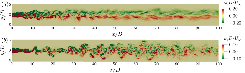
Figure 2: Instantaneous snapshot of vertical vorticity at the central horizontal plane ($z=0$): (a) $\mbox{{Fr}}=2$ and (b) $\mbox{{Fr}}=10$.

Figure 2 shows the instantaneous vertical vorticity ($\omega_{z}D/U_{\infty}$) on the central horizontal plane ($z=0$) for the $\mbox{{Fr}}=2$ (top) and $\mbox{{Fr}}=10$ (bottom) wakes. Similar to figure 1, $\omega_{z}$ is calculated using filtered velocity fields to emphasize large-scale features. In both wakes, the complex spatial distribution of vorticity in the immediate downstream of the disk gives way to a well-defined coherent distribution of opposite signed vortices in the intermediate to late wakes. For the $\mbox{{Fr}}=2$ wake, spatial coherence is visible as early as $x/D\approx 20$. Beyond $x/D\approx 20$, the regions of opposite-signed $\omega_{z}$ remain separated till the end of the domain. On closer inspection, a streamwise undulation of length $\lambda/D\approx 1/\mbox{{St}}_{VS}$ can be observed in figure 2(a). At this point, it is important to emphasize that the $\mbox{{Fr}}=2$ wake remains actively turbulent throughout the computational domain as demonstrated by CS2020 through spectra and visualizations of the turbulent dissipation rate. From $x/D\approx 40$ onward, the $\mbox{{Fr}}=2$ wake resides in the strongly stratified turbulent (SST) regime. Different regimes of stratified turbulence are discussed briefly in §1. The strong signature of coherence in the $\mbox{{Fr}}=2$ wake is not a consequence of the transition into the weakly turbulent state of the Q2D regime noted in previous works, e.g. by Spedding (1997).

The $\mbox{{Fr}}=10$ wake also shows a distinct wavy motion with non-dimensional wavelength $\approx 1/\mbox{{St}}_{VS}$. However, the separation between the regions with opposite signed vorticity is not as well defined as in the $\mbox{{Fr}}=2$ wake. According to CS2020, the $\mbox{{Fr}}=10$ wake stays in the weakly stratified regime (WST) from $x/D\approx 10$ to $50$ and thereafter stays in the intermediately stratified regime (IST) till the end of the domain.

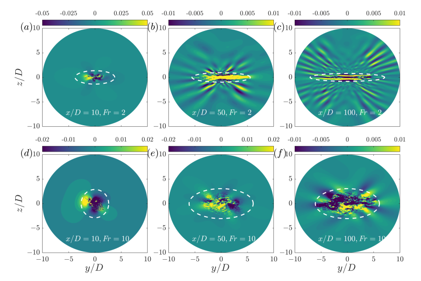
Figure 3: Instantaneous snapshots of the fluctuating spanwise velocity $u^{\prime}_{y}/U_{\infty}$ shown for $\mbox{{Fr}}=2$ (top row) and $\mbox{{Fr}}=10$ (bottom row): (a,d) at $x/D=10$, (b,e) at $x/D=50$, and (c,f) at $x/D=100$. Dashed close curve in white shows wake core.

To conclude this section, instantaneous snapshots of fluctuating spanwise velocity ($u^{\prime}_{y}/U_{\infty}$) are shown in figure 3 at locations in the near, intermediate and far wake at $\mbox{{Fr}}=2$ (top row) and $\mbox{{Fr}}=10$ (bottom row). An ellipse with major and minor axes equal to $2L_{Hk}$ and $2L_{Vk}$, where $L_{Hk}$ and $L_{Vk}$ are the TKE-based wake widths in horizontal and vertical directions, respectively, is also shown. $L_{Hk}$ is defined by $\mathrm{TKE}(x,y=L_{Hk},z=0)=\mathrm{TKE}(x,r=0)/2$ and $L_{Vk}$ by $\mathrm{TKE}(x,y=0,z=L_{Vk})=\mathrm{TKE}(x,r=0)/2$. Here, $r=0$ denotes the disk centerline. It is worth noting that using the sum of TKE and TPE to define the wake widths (not shown here) result in values similar to $L_{Hk}$ and $L_{Vk}$ for both $\mbox{{Fr}}=2$ and $\mbox{{Fr}}=10$ wakes. Following CS2020, we use the TKE-based definitions in the rest of the results and discussions. This ellipse, based on $L_{Hk}$ and $L_{Vk}$, is used to approximately demarcate the wake core from the outer wake. In subsequent sections, this definition of the wake core will prove to be useful for the interpretation of some SPOD results.

At $\mbox{{Fr}}=2$, an appreciable effect of buoyancy is already present in the near wake as shown in figure 3(a) for $x/D=10$, which corresponds to $Nt_{2}=5$ in buoyancy time units. At the same streamwise location, the $\mbox{{Fr}}=10$ wake still has a circular cross-section with an imprint of the $m=1$ azimuthal mode which was found to be energetically important in the unstratified wake (Nidhan et al. (2020)). As both the wakes evolve downstream, buoyancy has a progressively increasing effect on the the wake core as well as the surrounding outer wake. By $x/D=50$, vertically flattened wake cores can be observed in figure 3(b,d) for both the wakes, more so at $\mbox{{Fr}}=2$ than at $\mbox{{Fr}}=10$. It is also worth noting that the wake core of $\mbox{{Fr}}=2$ consists of distinct layers by $x/D=50$. The $\mbox{{Fr}}=2$ wake also shows a significant amount of IGW activity in the outer region, i.e. outside the ellipse in figure 3(b). Farther downstream at $x/D=100$, the $u^{\prime}_{y}$ field of $\mbox{{Fr}}=2$ (figure 3(c)) shows IGWs occupying a significant portion of the outer wake with the wake core being further flattened and comprising an increased number of horizontally oriented layers. The $\mbox{{Fr}}=10$ wake core also starts showing appreciable IGW activity in the ambient by $x/D=100$ ($Nt_{10}=10$), as shown in figure 3(f).

5 Characteristics of SPOD eigenvalues and eigenspectra

We start the discussion of SPOD modes by evaluating their overall contribution to fluctuation energy and by their eigenspectra. There are significant effects of buoyancy as elaborated below.

5.1 Cumulative modal contribution to fluctuation energy

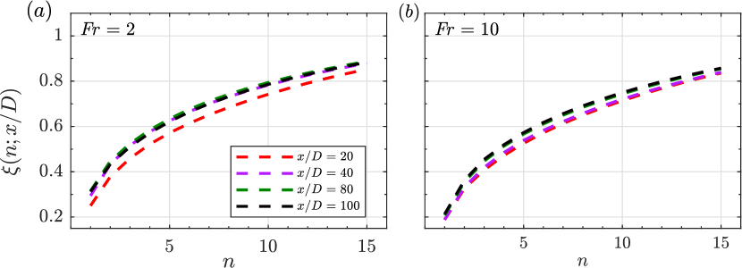
Figure 4: Variation of the cumulative energy, $\xi(n)$, as a function of modal index $n$ for (a) $\mbox{{Fr}}=2$ and (b) $\mbox{{Fr}}=10$ wakes, shown till $n=15$ SPOD modes.

Figure 4 shows the variation of cumulative energy ($\xi(n)$) as a function of SPOD modal index ($n$) at four downstream locations: $x/D=20,40,80,$ and $100$. To calculate $\xi(n)$, the energy across all resolved frequencies St at each modal index up to $n$ is summed and normalized by the total energy as follows:

$$\xi(n;x/D)=\frac{\sum\limits_{i=1}^{n}\sum_{St}\lambda^{(i)}(f;x/D)}{\sum\limits_{i=1}^{N_{blk}}\sum_{St}\lambda^{(i)}(f;x/D)},$$ (15)

where $N_{blk}$ is the total number of SPOD modes at a given St. Comparison among the various $x/D$ curves shows that the energy captured by leading SPOD modes in both wakes increases with downstream distance. This behavior is in contrast to the unstratified wake where the relative importance of the dominant SPOD modes decreases with increasing $x/D$ (Nidhan et al., 2020). Although both stratified wakes exhibit an increasing dominance of the leading modes as $x/D$ increases, there is a quantitative difference in that the jump of modal energy fraction from its $x/D=20$ value is larger for the the $\mbox{{Fr}}=2$ wake relative to the $\mbox{{Fr}}=10$ wake.

As discussed in the introduction, CS2020 found that the $\mbox{{Fr}}=2$ wake traversed the WST, IST and SST regimes during its streamwise evolution and the $\mbox{{Fr}}=10$ wake accessed only the WST and IST regimes. Readers are referred to §1 for an introduction to these regimes in stratified turbulence. These transitions also appear in the the evolution of the modal energy content $\xi(n;x/D)$. For example, the $\mbox{{Fr}}=2$ wake in figure 4(a) shows a transition at $x/D\approx 40$ whereby the $\xi(n)$ curves for $x/D\geq 40$ collapse onto a single profile. This result is consistent with CS2020 who find that $x/D\approx 40$ ($Nt_{2}\approx 20)$ is the location where the $\mbox{{Fr}}=2$ wake wake transitions from IST to SST. The $\mbox{{Fr}}=10$ wake was found by CS2020 to stay in the WST regime till $x/D\approx 50$ ($Nt\approx 5$) and thereafter transitioned to the IST regime. For the $\mbox{{Fr}}=10$ wake in figure 4(b), the $\xi(n)$ curves collapse separately, i.e. there is one curve showing collapse between $x/D=20$ and 40 which lie in the WST regime, and there is another showing collapse between $x/D=80$ and $100$ which lie in the IST regime. Plots of $\xi(n)$ at other values of $x/D$ (not shown here) confirm that locations with $x/D\leq 50$ collapse on the $x/D=20,40$ curve and locations with $x/D\geq 80$ collapse on the $x/D=80,100$ curve.

The energy summed over frequencies instead of modal indices is now examined. Figure 5 shows the variation of $\xi(\mbox{{St}})$ calculated as follows:

$$\xi(\mbox{{St}};x/D)=\frac{\sum\limits_{f=-St}^{St}\sum\limits_{i=1}^{N_{blk}}\lambda^{(i)}(f;x/D)}{\sum\limits_{i=1}^{N_{blk}}\sum_{St}\lambda^{(i)}(f;x/D)}.$$ (16)

Figure 5 shows that $\xi(\mbox{{St}})$ increases for low-St modes with increasing $x/D$ in both wakes, which is a trend also seen for $\xi(n)$. This is yet another indication of the increasing importance of the coherent modes as buoyancy effects come into play in these stratified wakes. Besides, for both wakes, $\xi(\mbox{{St}})$ increases steeply between $\mbox{{St}}=0.1$ and $0.2$ at all downstream locations. The reason behind this sharp increase will be discussed shortly. Another observation of interest is that almost all the fluctuation energy at large $x/D$ is captured by the modes with $\mbox{{St}}<1$ in both wakes.

From $x/D=20$ to $40$, there is a large jump in $\xi(\mbox{{St}})$ for the $\mbox{{Fr}}=2$ wake in figure 5(a). As mentioned previously, $x/D=40$ also marks the arrival of the $\mbox{{Fr}}=2$ wake into the SST regime. Also, the $\xi(\mbox{{St}})$ curves collapse for locations $x/D=80$ and $100$. On analyzing other streamwise locations (not shown here), we find that the $\xi(\mbox{{St}})$ curves for $x/D\geq 70$ collapse together similar to the previously shown $\xi(n)$ curves of the $\mbox{{Fr}}=2$ wake. One difference is that the collapse of $\xi(n)$ commences closer to the body at $x/D\approx 40$.

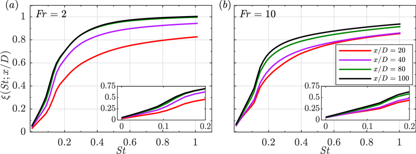
Figure 5: Variation of the cumulative fraction of energy, $\xi(\mbox{{St}})$, as a function of St for (a) $\mbox{{Fr}}=2$ and (b) $\mbox{{Fr}}=10$. The plots are shown for $0\leq\mbox{{St}}\leq 1$ for both cases. Inset plots show zoomed-in variation of $\xi(\mbox{{St}})$ for $0\leq\mbox{{St}}\leq 0.2$.

Contrary to the $\mbox{{Fr}}=2$ wake where the change in $\xi(\mbox{{St}})$ from $x/D=20$ to $x/D=40$ was large, the corresponding change for the $\mbox{{Fr}}=10$ wake (figure 5(b)) is small and consistent with an absence of regime change. However, the $\mbox{{Fr}}=10$ wake exhibits a significant jump of $\xi(\mbox{{St}})$ between $x/D=40$ and $80$, which lie in the WST and IST regime, respectively.

To summarize, figures 4 and 5 have the following implications. First, the relative importance of the leading SPOD modes increases with $x/D$ for the stratified wakes, which is in stark contrast to their behavior in the unstratified wake (Nidhan et al. (2020)). Second, the trend of increasing dominance of leading SPOD modes is more pronounced for the strongly stratified wake of $\mbox{{Fr}}=2$ as compared to $\mbox{{Fr}}=10$. Third, transitions between WST, IST and SST regimes discussed by CS2020 for the turbulence statistics are also qualitatively reflected in the energetics of SPOD modes too.

5.2 SPOD eigenspectra of $\mbox{{Fr}}=2$ and $10$ wakes

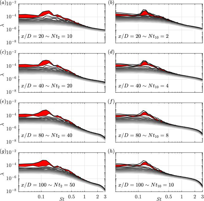
Figure 6: SPOD eigenspectra of 25 most energetic modes, $\lambda^{(1)}$ to $\lambda^{(25)}$, for the $\mbox{{Fr}}=2$ (left column) and $\mbox{{Fr}}=10$ (right column) wakes at four streamwise locations: (a,b) $x/D=20$, (c,d) $x/D=40$, (e,f) $x/D=80$, and (g,h) $x/D=100$. Dark to light shade corresponds to increasing model index $i$ in $\lambda^{(i)}$.

Figure 6 shows the SPOD eigenspectra of the $\mbox{{Fr}}=2$ (left column) and $\mbox{{Fr}}=10$ (right column) wakes at various downstream locations. The spectrum of the leading SPOD mode ($\lambda^{(1)}$) shows a distinct spectral peak in the vicinity of $\mbox{{St}}=0.13-0.15$ at all locations and for both wakes. This pronounced peak is the reason why there was a sharp increase of $\xi(\mbox{{St}})$ within $0.1<\mbox{{St}}<0.2$ for both wakes in figure 5.

In the $\mbox{{Fr}}=10$ wake, the $\lambda^{(1)}$ eigenspectrum at all locations has a distinct peak at $\mbox{{St}}\approx 0.13$, which is very close to the vortex shedding (VS) frequency of the unstratified wake ($\mbox{{St}}=0.135$) at the same Reynolds number (Nidhan et al. (2020)). SPOD eigenspectra at $x/D<2$ (not presented here) show that this spectral peak has its origin near the wake generator and corresponds to vortex shedding in the $\mbox{{Fr}}=10$ wake.

Unlike the $\mbox{{Fr}}=10$ wake, the spectral peak in $\lambda^{(1)}$ for the $\mbox{{Fr}}=2$ wake shifts slightly from $\mbox{{St}}\approx 0.15$ at $x/D=20$ to $\mbox{{St}}\approx 0.13$ at $x/D=40$ and onward. At the far wake location of $x/D=80$, the peak in the $\lambda^{(1)}$ eigenspectrum broadens to reach $\mbox{{St}}\approx 0.11$. Near-body SPOD eigenspectra (not shown here) for the $\mbox{{Fr}}=2$ wake show a prominent peak at $\mbox{{St}}\approx 0.15$ (slightly larger relative to the unstratified and $\mbox{{Fr}}=10$ wakes) just downstream of the recirculation zone at $x/D\approx 2$. Furthermore the pressure spectrum (not presented here) in the immediate proximity of the disk, at $x/D=0.5$ and $r/D=0.5$, also peaks at $\mbox{{St}}\approx 0.15$, indicating that this frequency corresponds to the VS mechanism for the $\mbox{{Fr}}=2$ wake. The shift in the spectral peak towards lower St at later $x/D$ is consistent with the sphere-wake study of Spedding (2002a) who report a gradual reduction in the dominant wake St during $40<Nt<100$ (see figure 5 of their paper).

In the $\mbox{{Fr}}=2$ wake, there is a large gap (demarcated in red) between the $\lambda^{(1)}$ and $\lambda^{(2)}$ spectra for frequencies with $\mbox{{St}}<0.2$. Beyond $\mbox{{St}}\approx 0.2$, values of all $\lambda^{(i)}$ fall sharply. This large difference between $\lambda^{(1)}$ and $\lambda^{(2)}$ implies that the dynamics of the $\mbox{{Fr}}=2$ wake is low-rank, i.e. it is dominated by the leading SPOD mode. The sharp drop-off in energy at higher St points to the dominance of low-frequency energetic structures with St in $[0,0.2]$, specifically around the VS frequency.

In terms of low-rank behavior, the $\mbox{{Fr}}=10$ wake shows a peculiar difference from the $\mbox{{Fr}}=2$ wake. Although the gap between $\lambda^{(1)}$ and $\lambda^{(2)}$ is significantly less compared to that for $\mbox{{Fr}}=2$, there is a significant gap between $\lambda^{(2)}$ and $\lambda^{(3)}$ around the VS frequency $\mbox{{St}}\approx 0.13$, shown in red in the right column of figure 6. Furthermore, the variation of $\lambda^{(2)}$ with St is very similar to that of $\lambda^{(1)}$. On further investigation, we find that the SPOD eigenmodes of $\lambda^{(1)}$ and $\lambda^{(2)}$ at the VS frequency have similar spatial structure, but with a rotation in their orientation. We hypothesize that $\lambda^{(1)}$ and $\lambda^{(2)}$ modes at the VS frequency are the manifestation of $m=1$ and $m=-1$ azimuthal modes in the weakly stratified $\mbox{{Fr}}=10$ wake.

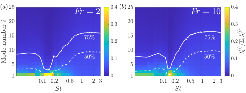
Figure 7: Fraction of energy (at a given St) accounted by each SPOD mode as a function of frequency at $x/D=50$ for: (a) $\mbox{{Fr}}=2$ and (b) $\mbox{{Fr}}=10$ wakes. The solid and dashed white lines indicate the number of SPOD modes required to retain 75% and 50% of the total fluctuation energy respectively at each frequency.

Figure 7 shows the fraction of energy in each SPOD mode as a function of St for both wakes at a representative location of $x/D=50$. In both wakes, the leading SPOD mode at the VS frequency capture at least $40\%$ of the total energy contained in the VS frequency. This also holds true for the near ($x/D=10$) and far ($x/D=100$) locations in both wakes (not discussed here for brevity). Also, in both, wakes, less than 5 SPOD modes are required to capture $75\%$ of the total energy in the vicinity of the VS frequency, as indicated by the solid white line in figure 7.

The key takeaway from figure 6 and figure 7 is twofold: (i) the VS frequency is the leading contributor to the fluctuating energy content of both $\mbox{{Fr}}=2$ and $10$ wakes and (ii) its dynamics are primarily governed by a few leading SPOD modes. Previous experimental studies of Chomaz et al. (1993) and Lin et al. (1992a) have showed the existence of the VS mode in the near wake at moderate stratification using hot-wire measurements (at few select locations) and shadowgraph techniques. The present SPOD analysis enables us to establish the dominance of the VS mode in stratified wakes from near the body to 100 body diameters downstream by providing an ordered set of $\lambda^{(i)}$ eigenvalues for different St.

6 The energetics of the vortex shedding (VS) mode

A comparison between SPOD eigenspectra of the stratified wakes (figure 6) and the unstratified wake (figure 3 in Nidhan et al. (2020)) reveals that both types of wakes are dominated by vortex shedding which gives rise to a distinct spectral peak in the vicinity of $\mbox{{St}}\approx 0.13$. For the unstratified wake, besides the VS structure, which appears in the azimuthal mode $m=1$, a double helix ($m=2$) mode with a peak at $\mbox{{St}}\rightarrow 0$ is also found to be energetically important (Johansson & George, 2006; Nidhan et al., 2020). In the stratified wake, as elaborated below, we find that the VS mode is persistent, is linked to unsteady internal gravity waves (IGWs), and is thereby responsible for the accumulation of fluctuation energy outside the wake core.

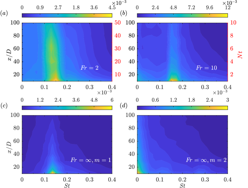
Figure 8: $x/D-\mbox{{St}}$ contour maps showing the variation of total energy in the leading 15 SPOD modes: (a) $\mbox{{Fr}}=2$, (b) $\mbox{{Fr}}=10$, (c) $\mbox{{Fr}}=\infty$, $m=1$ (vortex shedding) mode, and (d) $\mbox{{Fr}}=\infty$, $m=2$ (double helix) mode. The contour level of each plot is set between zero and the maximum value of the energy over all $(x/D,\mbox{{St}})$ pairs in that plot. Results for $\mbox{{Fr}}=\infty$ wake are taken from Nidhan et al. (2020).

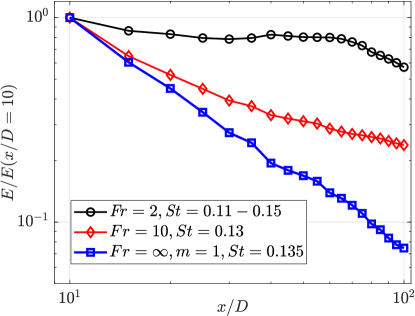
Figure 9: Evolution of the energy contained in leading 15 SPOD modes at the vortex shedding frequency is shown for $\mbox{{Fr}}=2,10$, and $\infty$ wakes. The energy is normalized by its value at $x/D=10$. Energy across $0.11\leq\mbox{{St}}\leq 0.15$ is summed for the $\mbox{{Fr}}=2$ wake since it has a broader spectral peak (see figure 6).

Stratification qualitatively affects the streamwise evolution of the energy in different frequencies. The evolution of the frequency-binned energy is shown for the stratified wakes in figure 8 (a)-(b). For the unstratified case ($\mbox{{Fr}}=\infty$), the azimuthal modes $m=1$ and $m=2$ are shown in figure 8(c) and (d), respectively. For the stratified wakes in figures 8 (a)-(b), the spectral peak in the vicinity of $\mbox{{St}}\approx 0.13$ remains prominent for significant downstream distances, especially for $\mbox{{Fr}}=2$. A somewhat wide band ($0.1\leq\mbox{{St}}\leq 0.2$), centered around $\mbox{{St}}\approx 0.13$ of the VS mode, is excited for the stratified wakes. Furthermore, this band persists into the far wake. Even at $x/D=100$, this band has larger energy density than at other frequencies. Such persistence in the energetic dominance of the VS mode (and neighboring frequencies) is absent in the unstratified $\mbox{{Fr}}=\infty$ case where the energy at the two peaks of: (i) $\mbox{{St}}=0.135$ in the $m=1$ mode (figure 8(a)) and (ii) $\mbox{{St}}=0$ in the $m=2$ mode (figure 8(b)) declines sharply with increasing $x/D$.

Figure 9 shows the streamwise evolution of energy in the leading 15 SPOD modes and in a frequency band around the VS frequency. The energy in the $\mbox{{Fr}}=2$ wake remains almost constant till $x/D=60$ and starts decaying slowly thereafter. On the other hand, the $\mbox{{Fr}}=10$ wake shows an initial decay in the VS mode energy which closely follows that of the $\mbox{{Fr}}=\infty$ wake till $x/D=20$. Subsequently, buoyancy effects set in for the $\mbox{{Fr}}=10$ wake to slow down the energy decay.

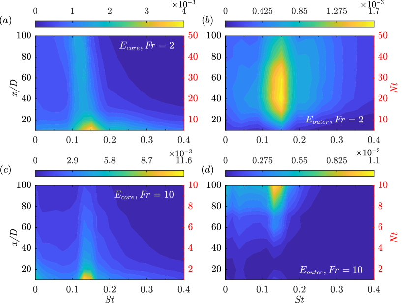
Figure 10: Energy partition between core and outer wake: (a) wake core of $\mbox{{Fr}}=2$, (b) outer wake of $\mbox{{Fr}}=2$, (c) wake core of $\mbox{{Fr}}=10$, and (d) outer wake of $\mbox{{Fr}}=10$. The first 15 SPOD modes are considered and the contour level of each plot is set between zero and the maximum value of the energy over all $(x/D,\mbox{{St}})$ pairs in that plot.

To investigate the reason behind the downstream persistence of the VS spectral peak in stratified wakes, the total energy in the leading 15 SPOD modes is partitioned into two components: (i) energy of the wake core, $E_{core}$ and (ii) energy of the outer wake, $E_{outer}$. The energy in each of the regions is calculated as:

$$E_{core}(x/D,\mbox{{St}})=\sum\limits_{n=1}^{15}\ \int\limits_{A\in\Omega}\lambda^{(n)}(x/D,\mbox{{St}})\Phi^{*(n)}_{i}(x/D,\mbox{{St}})\Phi^{(n)}_{i}(x/D,\mbox{{St}})\mathop{}\!\mathrm{d}A,$$ (17)

$$E_{outer}(x/D,\mbox{{St}})=\sum\limits_{n=1}^{15}\ \int\limits_{A\in\mathcal{H}-\Omega}\lambda^{(n)}(x/D,\mbox{{St}})\Phi^{*(n)}_{i}(x/D,\mbox{{St}})\Phi^{(n)}_{i}(x/D,\mbox{{St}})\mathop{}\!\mathrm{d}A,$$ (18)

where $\Omega$ denotes the wake core at a given $x/D$, as defined in §4. $\mathcal{H}$ denotes the area of the circular cross-section bounded by $0\leq r/D\leq 10$ at a given $x/D$. Here, $\Phi^{(n)}_{i}$ corresponds to the $n^{th}$ SPOD eigenmode for a given $x/D$ and St.

The energy in the wake core peaks around the VS-mode frequency, $\mbox{{St}}\approx 0.12-0.13$, for both wakes (see figure 10(a,c)). With increasing $x/D$ (or $Nt$), the VS signature in the wake core decays for both wakes. The energetics of the outer wake is remarkably different. $E_{outer}$, which starts off with a small value across all St at $x/D\approx 10$ in the $\mbox{{Fr}}=2$ wake, develops a peak at $\mbox{{St}}\approx 0.15$ at $x/D\approx 20$. Note that this peak is the same as the peak in the SPOD eigenspectrum for the entire wake (figure 6(a)). Farther downstream, there is significant energy content in the outer wake for $x/D\approx 16-80$ ($Nt_{2}\approx 8-40$) with a spectral peak located at $\mbox{{St}}\approx 0.13-0.15$. The spectral peak is broad, i.e. nearby frequencies with $0.1\leq\mbox{{St}}\leq 0.2$ also have comparable energy levels. For the $\mbox{{Fr}}=10$ wake, $E_{outer}$ picks up only beyond $x/D=60$ ($Nt_{10}=6$), and thereafter increases progressively in the vicinity of $\mbox{{St}}\approx 0.13$ till the end of the domain. We also find that the qualitative nature of the variation of energy in the outer wake and wake core found in figure 10 does not change when the number of modes over which energy is summed is decreased from 15 to 3 (not presented here for brevity).

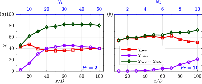
Figure 11: Streamwise variation of $\chi_{core}$, $\chi_{outer}$, and $\chi_{core}+\chi_{outer}$: (a) $\mbox{{Fr}}=2$, (b) $\mbox{{Fr}}=10$.

In figure 11, we sum up the SPOD energies across $\mbox{{St}}\in[-0.4,0.4]$ separately for the wake core and the outer wake and compute their percentage contribution to the entire area-integrated fluctuation energy as follows,

$$\chi_{core}(x/D)=\frac{\sum\limits_{|St|=[0,0.4]}E_{core}(\mbox{{St}},x/D)}{E_{k}^{T}(x/D)+E_{\rho}^{T}(x/D)}\times 100,$$ (19)

$$\chi_{outer}(x/D)=\frac{\sum\limits_{|St|=[0,0.4]}E_{outer}(\mbox{{St}},x/D)}{E_{k}^{T}(x/D)+E_{\rho}^{T}(x/D)}\times 100,$$ (20)

where $E^{T}_{k}(x/D)$ and $E^{T}_{\rho}(x/D)$ are area-integrated TKE and TPE in the circular region of $0\leq r/D\leq 10$ at the $x/D$ location under consideration. The streamwise evolution of $\chi_{core}$ and $\chi_{outer}$ are shown in figure 11.

For the $\mbox{{Fr}}=2$ wake (figure 11(a)), $\chi_{outer}$ increases monotonically until $x/D\approx 60$ followed by a slight decrease. At its peak, $\chi_{outer}$ constitutes up to $50\%$ of the total fluctuation energy, becoming even larger than $\chi_{core}$. In the $\mbox{{Fr}}=10$ wake (figure 11(b)), $\chi_{outer}$ remains negligible till $x/D=60$, followed by a monotonic increase. The increase in the value of $\chi_{outer}$ is accompanied by a decrease in the wake-core contribution. The percentage of total energy captured by the leading 15 SPOD modes and $|\mbox{{St}}|\in[0,0.4]$, i.e., $\chi_{wake}+\chi_{outer}$ (shown in green), increases for both wakes from its initial value at $x/D=10$. This reinforces a main finding of this work that stratified wakes display an increased coherence of fluctuation energy as they evolve downstream.

Figure 10 suggests that the unsteady IGWs in the outer wake radiate from the VS mode at intermediate to late $Nt$. Nevertheless, to further establish causation between the unsteady IGW emission and the VS mode, we perform additional SPOD analyses for the $\mbox{{Fr}}=2$ wake. In these analyses, we replace the fluctuating density field $\rho^{\prime}$ with the fluctuating pressure field $p^{\prime}$. These SPOD analyses are performed at $x/D=10,20,\cdots,90,100$. At all locations, the eigenspectra obtained from these modified SPOD analyses show a prominent peak at the VS frequency with a large gap between $\lambda^{(1)}$ and $\lambda^{(2)}$ for $\mbox{{St}}<0.2$, qualitatively akin to the left column of figure 6.

Using $p^{\prime}$ along with $u^{\prime}_{i}$ enables us to reconstruct the pressure transport term in the radial direction, $\langle p^{\prime}u^{\prime}_{r}\rangle$, which accounts for the energy transferred radially from the wake core to the IGW dominated outer wake region through pressure-work (de Stadler & Sarkar, 2012; Rowe et al., 2020). We reconstruct $\langle p^{\prime}u^{\prime}_{r}\rangle$ contours using leading 15 SPOD modes and frequencies in the range of (i) $\mbox{{St}}\in[0.1,0.2]$ and (ii) $\mbox{{St}}\in[0.1,0.3]$ as follows:

$$\langle p^{\prime}u^{\prime}_{r}\rangle(x;y,z)=\sum\limits_{St}\sum\limits_{n=1}^{15}\lambda^{(n)}(x;\mbox{{St}})\,\Phi_{u_{r}}^{(n)}(x;y,z,\mbox{{St}})\,\Phi_{p}^{(n)*}(x;y,z,\mbox{{St}}),$$ (21)

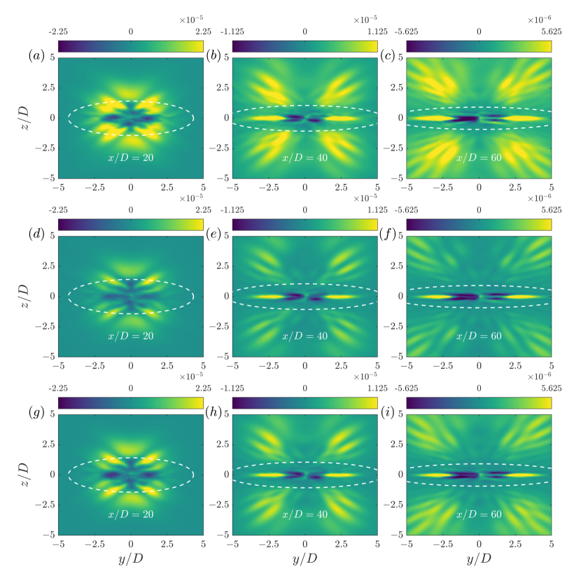
Figure 12: Contours of $\langle p^{\prime}u^{\prime}_{r}\rangle$ for the $\mbox{{Fr}}=2$ wake obtained from: (i) temporal averaging (top row), reconstruction using leading 15 SPOD modes and (ii) $\mbox{{St}}\in[0.1,0.2]$ (middle row) and (iii) $\mbox{{St}}\in[0.1,0.3]$ (bottom row). Three streamwise locations $x/D=20,40,$ and $60$ are shown. Dashed closed curve in white shows wake core.

Figure 12 shows the actual (top row) and reconstructed (middle and bottom rows) $\langle p^{\prime}u^{\prime}_{r}\rangle$ at three streamwise locations $x/D=20,40,$ and $60$ for the $\mbox{{Fr}}=2$ wake. The actual $\langle p^{\prime}u^{\prime}_{r}\rangle$ shows a strong signature of IGW flux in the outer wake region at all three downstream locations in figure 12. We found that the nonlinear transport term was negligible outside the wake core (not shown here). Hence the primary source of the energy transfer to the outer wake is the pressure-work term due to the IGW radiation. The reconstructed $\langle p^{\prime}u^{\prime}_{r}\rangle$ using $\mbox{{St}}\in[0.1,0.2]$ (middle row) shows qualitative agreement with the spatial distribution of actual $\langle p^{\prime}u^{\prime}_{r}\rangle$, both in the wake core as well as outer wake region, at all downstream locations. As more frequencies are included (bottom row), adjacent to the VS frequency, the accuracy of reconstruction increases. The key spatial characteristics of $\langle p^{\prime}u^{\prime}_{r}\rangle$ remain similar in both reconstructions, showing that frequencies in the vicinity of the VS frequency satisfactorily capture the key dynamics of unsteady IGW generation.

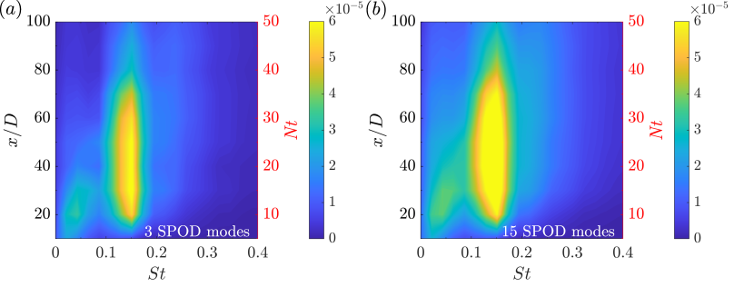
Figure 13: $x/D-\mbox{{St}}$ contour maps showing the variation of integrated $\langle p^{\prime}u^{\prime}_{r}\rangle$ in the outer wake region using: (a) leading 3 SPOD modes and (b) leading 15 SPOD modes for the $\mbox{{Fr}}=2$ wake.

To further elucidate the causal link between the VS mode and the IGW generation, we plot the $x/D-\mbox{{St}}$ variation of the integrated $\langle p^{\prime}u^{\prime}_{r}\rangle$ in the outer wake region (similar to 18), reconstructed using 3 and 15 SPOD modes (figure 13). The evolution of integrated $\langle p^{\prime}u^{\prime}_{r}\rangle$ in the outer wake of the $\mbox{{Fr}}=2$ wake is very similar to that of the energy in the outer wake region (figure 10(b)). It starts off at a small value at $x/D\approx 10$, develops a broad peak centered at $\mbox{{St}}\approx 0.15$ between $20\leq x/D\leq 80$, and gradually starts declining beyond $x/D=80$. Increasing the number of modes from $3$ to $15$ makes the active St region broader while intensifying the reconstructed values.

Figure 10, 12, and 13 firmly establish that the VS mode energy radiates out of the wake core instead of being acted on by nonlinear interactions in the turbulent wake responsible for the usual energy cascade. Therefore, unlike their unstratified counterpart, the stratified wakes exhibit a persistent VS spectral peak when the energy in the full domain of influence (denoted by $\mathcal{H}$) of the wake is taken into account as in the SPOD results of figure 8(a,b).

7 Spatial structure of SPOD eigenmodes

7.1 Spatial structure of the VS eigenmode

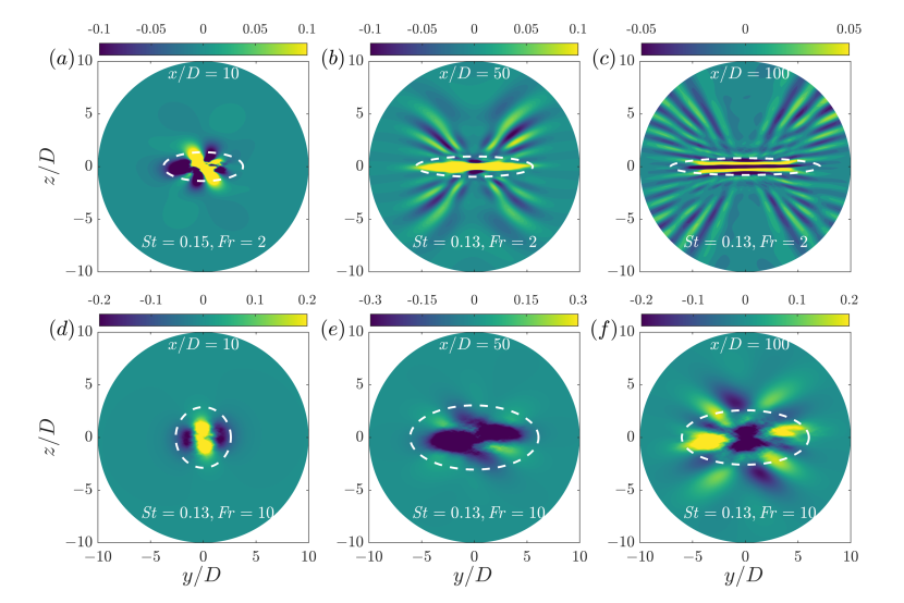
Figure 14: Shape of the leading SPOD mode (real part corresponding to $\lambda^{(1)}$) for spanwise velocity, $\Phi^{(1)}_{y}(y,z,\mbox{{St}};x/D)$: (a) $x/D=10,\mbox{{Fr}}=2,\mbox{{St}}=0.15$, (b) $x/D=50,\mbox{{Fr}}=2,\mbox{{St}}=0.13$, (c) $x/D=100,\mbox{{Fr}}=2,\mbox{{St}}=0.13$, (d) $x/D=10,\mbox{{Fr}}=10,\mbox{{St}}=0.13$, (e) $x/D=50,\mbox{{Fr}}=10,\mbox{{St}}=0.13$, and (f) $x/D=100,\mbox{{Fr}}=10,\mbox{{St}}=0.13$. At each $x/D$, the shown mode corresponds to the peak in the eigenspectrum of $\lambda^{(1)}$. Real part of each mode is shown. Dashed closed curve in white shows wake core.

The spatial structure of the dominant eigenmodes sheds further light on the manner in which buoyancy helps spread unsteady flow perturbation to well outside the turbulent core of the wake. Figure 14 shows the real part of the normalized (by $L_{\infty}$ norm) leading SPOD mode, $\Phi^{(1)}_{y}(y,z,\mbox{{St}};x)/||\Phi^{(1)}_{y}(y,z,\mbox{{St}};x)||_{\infty}$, of the lateral velocity $u_{y}$. The plotted modes correspond to the VS mode, which is at St corresponding to the eigenspectrum peak and are shown for selected values of $x/D$. The ellipsoid wake core (dashed blue curve) with dimensions $2L_{Hk}$ and $2L_{Vk}$ is also shown. At $\mbox{{Fr}}=2$ (upper row), the wake core exhibits flattening from $x/D=10$ ($Nt=5$) onward and the eigenmodes in the core show horizontal layering for $x/D\geq 50$. The layering becomes visible in the eigenmodes at $x/D\approx 30$ (not shown here). The region outside the core has little activity at $x/D=10$ but shows IGW phase lines at $x/D=50$ and 100. There is a clear and continuous transition of the eigenmode from its layered core to an IGW structure in the outer region at the far downstream locations. The flattening of the wake core and the IGW related spread of the eigenmode is delayed for the $\mbox{{Fr}}=10$ wake (bottom row) relative to $\mbox{{Fr}}=2$ since equivalent $Nt$ values occur farther downstream.

Comparing figure 14(b,c) with figure 3(b,c), there are striking similarities in the layered structure of the $\mbox{{Fr}}=2$ wake core between the dominant eigenmodes and the instantaneous snapshots at the far downstream locations of $x/D=50$ and $100$. Although SPOD only guarantees that the obtained modes optimally capture the prescribed energy norm of the flow (see §3.1), these modes do generally contain the imprints of actual flow structures, as is the case here. The outer wake shows that distinct IGWs are associated with the wake core structure of dominant eigenmodes at late $Nt$ for both $\mbox{{Fr}}=2$ and $10$ wakes. For the $\mbox{{Fr}}=2$ wake, IGW activity in the outer region of the eigenmodes shown in figure 14 is negligible at $x/D=10$ ($Nt_{2}=5$) while it is readily noticeable at $x/D=50$ ($Nt_{2}=25$) and $x/D=100$ ($Nt_{2}=50$). The IGWs are found to be emitted within $30^{\circ}-60^{\circ}$ with the $y$ axis. For $\mbox{{Fr}}=10$, the IGWs found at $x/D=100$ ($Nt_{10}=10$) are emitted at $\approx 45^{\circ}$ from the horizontal. A comparison between figure 3 and 14 reveals that the IGW in the dominant eigenmodes (figure 14) represent the IGWs in actual snapshots (figure 3) to a satisfactory extent, emphasizing that the VS mechanism is an important IGW generation mechanism in stratified wakes. The leading VS modes at different locations show asymmetry about the $y=0$ line, in both $\mbox{{Fr}}=2$ (at $x/D=10$) and $\mbox{{Fr}}=10$ (at $x/D=50$ and $100$) wakes. This could be a consequence of the presence of a very-low frequency mode in the wake (Grandemange et al., 2013; Rigas et al., 2014).

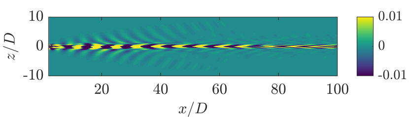
Figure 15: Shape of the leading SPOD mode for spanwise velocity, $\Phi^{(1)}_{y}(x,z,\mbox{{St}}\approx 0.13;y=0)$ in the center-vertical plane for the $\mbox{{Fr}}=2$ wake. Real part of the mode is shown in domain $z,x\in[-10,10]\times[2,100]$.

To analyze the streamwise coherence of the leading SPOD eigenmode at the VS frequency, we conduct an additional SPOD analysis for the $\mbox{{Fr}}=2$ wake, using the fluctuating density and velocity fields, at the center-vertical plane ($y=0$). Specific details of this SPOD analysis are mentioned towards the end of §3.2. The SPOD eigenspectrum (not shown here for brevity) shows a broad peak at $\mbox{{St}}\approx 0.13$ .

Figure 15 shows the spatial structure of the spanwise component of the leading SPOD mode at $\mbox{{St}}\approx 0.13$. The VS mode appears to be strongly coherent in the streamwise direction with a wavelength of $\lambda/D\approx 1/St_{VS}$. It has two distinctive features: (i) emergence of a well-defined IGW signature beyond $x/D\approx 20$ and (ii) gradual transition of the opposite signed lobes into V-shaped structures as the wake progresses downstream. These structures get progressively thinner and shallower (with respect to $x$ axis) as $x/D$ increases.

7.2 Spatial structure of high St, high $n$ eigenmodes

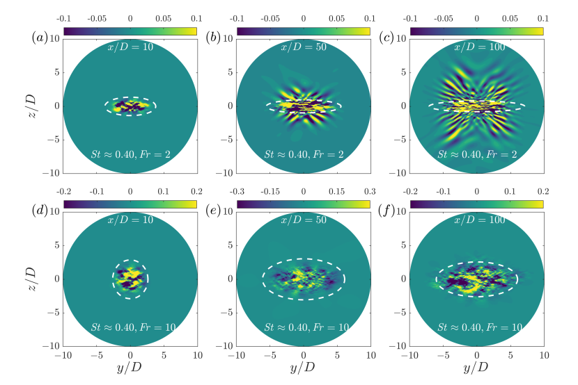
Figure 16: Shape of the $15^{th}$ SPOD mode (real part corresponding to $\lambda^{(15)}$) at $\mbox{{St}}=0.40$ for spanwise velocity, $\Phi^{(15)}_{y}(y,z,\mbox{{St}};x/D)$: (a) $x/D=10,\mbox{{Fr}}=2$, (b) $x/D=50,\mbox{{Fr}}=2$, (c) $x/D=100,\mbox{{Fr}}=2$, (d) $x/D=10,\mbox{{Fr}}=10$, (e) $x/D=50,\mbox{{Fr}}=10$, and (f) $x/D=100,\mbox{{Fr}}=10$. Dashed closed curve in white shows the wake core.

To contrast the structure of less energetic SPOD eigenmodes with the dominant SPOD eigenmodes, the $u_{y}$ eigenmode at $n=15$ and $\mbox{{St}}=0.40$ is plotted in figure 16 at the same downstream locations of $x/D=10,50$, and $100$ considered previously. It should be noted that these SPOD modes have low energy, $O(10^{-2})$ that of the dominant SPOD modes. Visual inspection shows that the spatial coherence in the wake core, which is a characteristic of dominant SPOD modes, is lost for the the high-$n$ and high-St modes similar to the result in the snapshot POD study of Diamessis et al. (2010). For both $\mbox{{Fr}}=2$ and $10$ wakes, $\Phi^{(15)}_{y}(y,z,\mbox{{St}}=0.40)$ in the wake core is dominated by small-scale turbulence. For the $\mbox{{Fr}}=2$ wake, the distinct layered structure found in the leading VS eigenmodes at $x/D=50$ and $100$ is absent in the low-energy mode at the same locations. Nevertheless, buoyancy-induced anisotropy is evident at $Nt\geq 5$ in both wakes even in these low-energy modes with high $n$ and St. Moreover, the $\Phi^{(15)}_{y}(y,z,\mbox{{St}}\approx 0.40)$ mode also shows IGWs in the outer wake at $x/D=50$ and $100$ in the $\mbox{{Fr}}=2$ wake (figure 16(b,c)), albeit with smaller wavelength than for the VS mode. Contrary to the $\mbox{{Fr}}=2$ wake, the $\Phi^{(15)}_{y}(y,z,\mbox{{St}}=0.4)$ mode for the $\mbox{{Fr}}=10$ wake does not show any IGW in figure 16(e,f).

8 Reconstruction using SPOD modes

In this section, we demonstrate the effectiveness of SPOD modes in reconstructing the following turbulence statistics: (i) turbulent kinetic energy (TKE), $\langle u^{\prime}_{i}u^{\prime}_{i}\rangle/2$, (ii) lateral production $\mathcal{P}_{xy}=\langle-u^{\prime}_{x}u^{\prime}_{y}\rangle\partial\langle U\rangle/\partial y$, and (iii) buoyancy flux $\mathcal{B}=\langle-\rho^{\prime}u^{\prime}_{z}\rangle/\mbox{{Fr}}^{2}$. The reconstruction from SPOD modes is performed as follows:

$$\mathop{}\!\mathrm{TKE}(x;y,z)=\frac{1}{2}\sum\limits_{n=1}^{\Lambda}\,\sum\limits_{\mbox{{St}}=-\mbox{{St}}_{r}}^{\mbox{{St}}=\mbox{{St}}_{r}}\lambda^{(n)}(x;\mbox{{St}})\,\Phi_{i}^{(n)}(x;y,z,\mbox{{St}})\,\Phi_{i}^{(n)*}(x;y,z,\mbox{{St}}),$$ (22)

$$\mathcal{P}_{xy}(x;y,z)=\sum\limits_{n=1}^{\Lambda}\,\sum\limits_{\mbox{{St}}=-\mbox{{St}}_{r}}^{\mbox{{St}}=\mbox{{St}}_{r}}-\lambda^{(n)}(x;\mbox{{St}})\,\Phi_{x}^{(n)}(x;y,z,\mbox{{St}})\,\Phi_{y}^{(n)*}(x;y,z,\mbox{{St}})\frac{\partial\langle U\rangle}{\partial y},$$ (23)

$$\mathcal{B}(x;y,z)=\frac{1}{\mbox{{Fr}}^{2}}\sum\limits_{n=1}^{\Lambda}\,\sum\limits_{\mbox{{St}}=-\mbox{{St}}_{r}}^{\mbox{{St}}=\mbox{{St}}_{r}}-\lambda^{(n)}(x;\mbox{{St}})\,\Phi_{\rho}^{(n)}(x;y,z,\mbox{{St}})\,\Phi_{z}^{(n)*}(x;y,z,\mbox{{St}}).$$ (24)

In (22$)-($24), the values of $\Lambda$ and $\mbox{{St}}_{r}$ determine the set of modes used for reconstruction. The so-obtained turbulence statistics vary spatially in spanwise and vertical directions for different $x/D$.

Throughout this section, two sets of low-order truncation are used for reconstruction: (i) $n\leq 5$, $|\mbox{{St}}|\leq 0.20$ (R1) and (ii) $n\leq 15$, $|\mbox{{St}}|\leq 0.40$ (R2). While the R1 truncation primarily takes the VS mode into account for both wakes, R2 also accounts for some of the low-energy modes which reside at relatively higher $n$ and St. It should be noted that R1 and R2 set of modes account for approximately 0.7% and 4.34% of the total SPOD modes in both wakes.

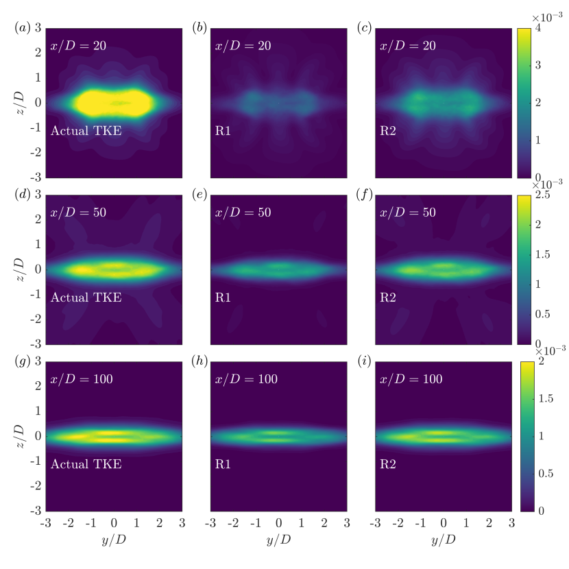
Figure 17: Contours of TKE for the $\mbox{{Fr}}=2$ wake obtained from temporal averaging (left column), reconstruction from R1 set of modes (middle column), and reconstruction from the R2 set of modes (right column). Three streamwise locations $x/D=20,50,$ and $100$ are shown.

Figure 17 compares the reconstructed TKE with its actual value for the $\mbox{{Fr}}=2$ wake at $x/D=20,50,$ and $100$. The actual TKE decays in magnitude, expands horizontally, and narrows vertically with increasing $x/D$. At $x/D=50$ and 100, the TKE contours display horizontal layering. At all three locations, reconstruction using the R1 set of modes (middle column) gives a fairly accurate estimate of the shape and spatial extent of the TKE contour. The layering at $x/D=50$ and $100$ is also captured by the R1 reconstruction. These layers were also present in the reconstruction using only $n=1$ and $|St|\leq 0.2$ modes (not shown here), indicating the low-rank nature of layering in stratified wakes. On further increasing $[n,\mbox{{St}}]$ as in the R2 reconstruction (right column), the overall shape and structural features of the reconstructed TKE remain unchanged, while the magnitude increases, particularly at intense TKE locations, increasing the overall accuracy. It can also be ascertained visually that the accuracy of R1 and R2 increases with downstream distance pointing to the increasing coherence of the wake as it progresses downstream.

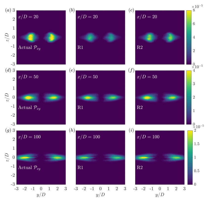
Figure 18: Contours of $\mathcal{P}_{xy}$ for the $\mbox{{Fr}}=2$ wake obtained from temporal averaging (left column), reconstruction from R1 set of modes (middle column), and reconstruction from R2 set of modes (right column). Three streamwise locations $x/D=20,50,$ and $100$ are shown.

Figure 18 pertains to the reconstruction of the lateral production $\mathcal{P}_{xy}$ in the $\mbox{{Fr}}=2$ wake. We limit ourselves to the lateral component since it dominates its vertical counterpart after the onset of buoyancy induced suppression of vertical turbulent motions (Brucker & Sarkar (2010); de Stadler & Sarkar (2012); Redford et al. (2015)). In the IST and SST regimes of the disk wake, $P_{xy}$ is the dominant component of turbulent production. The actual $\mathcal{P}_{xy}$ (left column) shows two off-axis lobes of intense production primarily located near the horizontal center plane ($z/D=0$). With increasing $x/D$, these lobes flatten owing to buoyancy. With respect to the lateral production, the R1 and R2 set of modes capture the spatial distribution accurately for the $\mbox{{Fr}}=2$ wake as shown in the middle and right column of figure 18, respectively. Although SPOD modes are optimal for capturing the area-integrated sum of $\langle u^{\prime}_{i}u^{\prime}_{i}\rangle$ and $\langle\rho^{\prime}\rho^{\prime}\rangle$/$\mbox{{Fr}}^{2}$ by construction, we find that these modes provides an excellent low-order approximation for the production too.

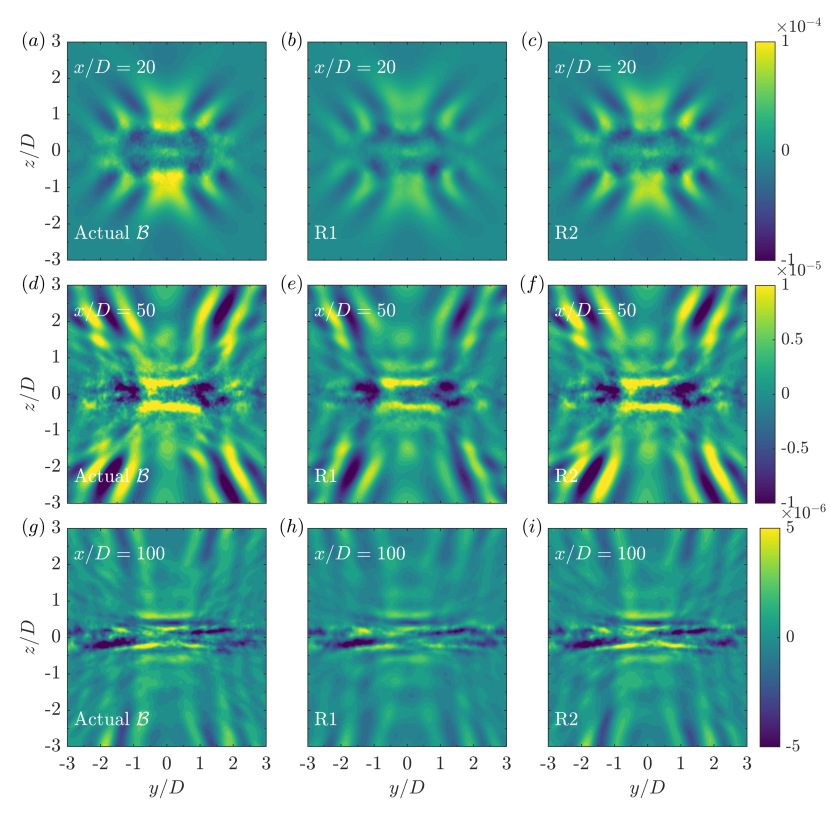
Figure 19: Contours of $\mathcal{B}$ for the $\mbox{{Fr}}=2$ wake obtained from temporal averaging (left column), reconstruction from R1 set of modes (middle column), and reconstruction from R2 set of modes (right column). Three streamwise locations $x/D=20,40,$ and $100$ are shown.

Finally, we explore the effectiveness of buoyancy flux ($\mathcal{B}$) reconstruction in figure 19. Unlike TKE and $\mathcal{P}_{xy}$, $\mathcal{B}$ is not a same-signed quantity in the turbulent wake, as can be seen from figure 19(a,d,g). The R1 reconstruction of $\mathcal{B}$ (middle column) accurately captures the structural features of $\mathcal{B}$ at all locations: (i) layers of positively and negatively signed $\mathcal{B}$ at $x/D=50$, $100$, and (ii) IGWs in the outer wake which carry significant $\mathcal{B}$ at $x/D=20$ and $50$. On closer inspection, the R1 truncation is found to underpredict the strength of $\mathcal{B}$ in these outer regions with intense buoyancy flux. Including higher St and $n$ modes for reconstruction, as done for R2, significantly improves the quality as shown in the right column.

The reconstruction trends of these statistical quantities are also investigated for the $\mbox{{Fr}}=10$ wake, but are not shown here for brevity. Qualitatively, the trends are similar to that of the $\mbox{{Fr}}=2$ wake, wherein the R1 set captures the structural features of these quantities very satisfactorily. Further addition of high-$n$ and high-St modes in the R2 truncation improves the quantitative prediction of these statistics, particularly in the region where they are found to be intense in the actual data.

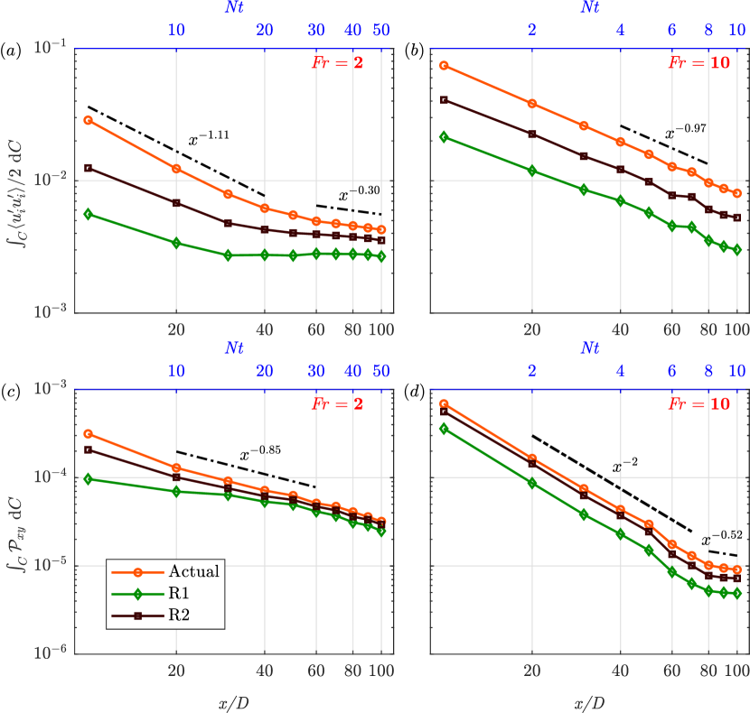
Figure 20: Streamwise variation of wake core TKE and $\mathcal{P}_{xy}$ reconstructed from R1 and R2 truncations: (a) TKE for $\mbox{{Fr}}=2$, (b) TKE for $\mbox{{Fr}}=10$, (c) $\mathcal{P}_{xy}$ for $\mbox{{Fr}}=2$, and (d) $\mathcal{P}_{xy}$ for $\mbox{{Fr}}=10$. Here, $\int_{C}\ (.)\mathop{}\!\mathrm{d}C$ denotes the integration in the wake core.

To conclude this section, the streamwise variations of the wake-core-integrated TKE and $\mathcal{P}_{xy}$ for the $\mbox{{Fr}}=2$ and $\mbox{{Fr}}=10$ wakes are shown in figure 20. The corresponding variation for $\mathcal{B}$ is not shown here as it fluctuates between small positive and negative values, unlike TKE and $\mathcal{P}_{xy}$ which decay monotonically with $x/D$.

For the $\mbox{{Fr}}=2$ wake, wake core TKE shows two distinct decay rates: (i) $\mathop{}\!\mathrm{TKE}\propto x^{-1.11}$ in the IST regime spanning $10\leq x/D\leq 40$ ($5\leq Nt_{2}\leq 20$) and (ii) $\mathop{}\!\mathrm{TKE}\propto x^{-0.30}$ in the SST regime spanning $60\leq x/D\leq 100$ ($30\leq Nt_{2}\leq 50$). The quality of TKE reconstruction improves monotonically from R1 to R2 at all downstream locations for both wakes, as is observed in figure 20(a,b). For $\mbox{{Fr}}=2$, the TKE contained in the R1 set of modes stays approximately constant for $x/D\geq 40$ (figure 20(a)). It is only after high-St and high-$n$ modes are added, as in R2, that the reconstructed TKE follows the decay rate of actual TKE. Reconstructed TKE from further lower-order truncations (not shown here), i.e., with lesser $n$ and St than in R1, showed an increase in wake core TKE at large $x/D$, opposite to the decrease in the actual value. For the $\mbox{{Fr}}=10$ wake, reconstruction from low-order truncations decay quite similar to the actual TKE (figure 20(b)).

The accuracy of R1 and R2 increase approximately three-folds and two-folds from $x/D=10$ to $100$ for the TKE reconstruction in the $\mbox{{Fr}}=2$ wake, suggesting development of low-rank dynamics in the $\mbox{{Fr}}=2$ wake. By $x/D=100$, R1 and R2 modes capture $\approx 63\%$ and $\approx 82\%$ respectively of the wake core TKE for $\mbox{{Fr}}=2$. On the other hand, the reconstruction quality of the moderately stratified $\mbox{{Fr}}=10$ wake changes only slightly from $x/D=10$ to $100$ for both low-order truncations: (i) TKE in R1 modes changes from $\approx 29\%$ of total TKE at $x/D=10$ to $\approx 38\%$ at $x/D=100$ and (ii) TKE in R2 modes change from $\approx 45\%$ to $\approx 55\%$ between $x/D=10$ and $100$.

Figure 20(c,d) show the reconstruction trends for wake core $\mathcal{P}_{xy}$ term in the $\mbox{{Fr}}=2$ and $10$ wakes, respectively, along with its actual variation obtained from temporal averaging (shown in red). The wake core $\mathcal{P}_{xy}$ for $\mbox{{Fr}}=2$ decays as $x^{-0.85}$ throughout the spatial domain under consideration (figure 20(c)). Both R1 and R2 provide very good reconstruction of $\mathcal{P}_{xy}$ beyond $x/D\approx 30$ and exhibit better approximations relative to that for TKE. With its additional modes, R2 follows the behavior of the actual value of $\mathcal{P}_{xy}$ very closely. The wake core $\mathcal{P}_{xy}$ for the $\mbox{{Fr}}=10$ wake shows a faster decay rate of $x^{-2}$ in $10\leq x/D\leq 70$ (figure 20(d)). Beyond $x/D\approx 80$, it decays at a slower rate of $x^{-0.52}$. Similar to the $\mbox{{Fr}}=2$ wake, R2 reconstructs the actual wake core $\mathcal{P}_{xy}$ very well.

The visually good reconstruction of $\mathcal{P}_{xy}$ by the R2 set of modes can be quantified for both wakes. At $x/D=10$ and $100$, R2 already accounts for $\approx 66\%$ and $\approx 92\%$ of the actual $\mathcal{P}_{xy}$, respectively, for the $\mbox{{Fr}}=2$ wake. For the $\mbox{{Fr}}=10$ wake, the R2 set of modes capture $\approx 80\%$ of the actual $\mathcal{P}_{xy}$ at both $x/D=10$ and $100$. The SPOD modes provide a better low-order truncation for the lateral production as compared to the TKE for both wakes. This is similar to the trend observed by Nidhan et al. (2020) for the unstratified wake at same $\Rey$.

9 Discussion and conclusions

In this study, we have extracted and analyzed coherent structures in the stratified turbulent wake of a disk using spectral POD (SPOD). Body-inclusive LES databases from Chongsiripinyo & Sarkar (2020) (referred to as CS2020) at $\Rey=5\times 10^{4}$ and $\mbox{{Fr}}=2,10$ are used in this study. Streamwise distance spanning $10\leq x/D\leq 100$ is analyzed for both wakes. The obtained SPOD eigenvalues ($\lambda^{(n)}$) are a function of modal index ($n$), frequency (St), and streamwise distance ($x/D$). By construction, SPOD modes have the following properties: (i) coherence in both space and time, (ii) optimal capture of the area-integrated total fluctuation energy, summed over kinetic and potential energy components, and (iii) ordering such that the energy content (given by $\lambda^{(n)}$) decreases with increasing $n$ for a given ($x/D,\mbox{{St}}$). To the best of the authors’ knowledge, this is the first numerical study utilizing SPOD and body-inclusive simulation data together to uncover the dynamics of coherent structures in high-$\Rey$ stratified wakes.

$Q$ criterion and vorticity visualizations of both $\mbox{{Fr}}=2$ and $10$ wakes give a qualitative indication of the prevalence of large-scale coherent structures in these wakes. SPOD analysis reveals their dominance, namely, the first five ($n=1$ to $5$) modes, summed across all resolved St, capture around 60% of the total fluctuation energy in both wakes. Likewise, most of the contribution to the total energy comes from SPOD modes with $\mbox{{St}}<1$ in both wakes. Contrary to the unstratified wake, the coherence in the stratified wakes increases with $x/D$. This is observed in both $n$ and St variation of the SPOD eigenvalues, wherein the relative contribution of the low $n$ and St eigenvalues increases with $x/D$. This increase in coherence is found to be more pronounced in the $\mbox{{Fr}}=2$ wake compared to the $\mbox{{Fr}}=10$ wake. Interestingly, the transitions between different turbulence regimes (WST, IST, and SST) in these wakes, discussed in detail by CS2020, are also reflected in the $n$ and St variations of the SPOD eigenvalues.

SPOD eigenspectra of both wakes at downstream locations ranging from the near to the far wake uncover a prominent spectral signature of the vortex shedding (VS) mechanism at $\mbox{{St}}\approx 0.11-0.13$. Both wakes exhibit a low-rank behavior in the vicinity of the vortex shedding frequency at all locations analyzed here, i.e. the leading modes have significantly higher energy content than the sub-optimal modes ($n>2$). While previous experimental studies of Lin et al. (1992b) and Chomaz et al. (1993) have shown the existence of the VS phenomenon in stratified wakes using qualitative visualizations and measurements of spectra at a few locations, SPOD enables us to objectively isolate and quantify the VS mechanism by providing the optimal decomposition of the two-point two-time cross-correlation matrix.

We also find that the $\mbox{{Fr}}=2$ wake exhibits the slowest decay of the energy at the VS frequency, followed by the $\mbox{{Fr}}=10$ and $\infty$ wakes, respectively. To further analyze this trend, the energy in the leading 15 SPOD modes is partitioned between the wake core and outer wake region for ($x/D,\mbox{{St}}$) pairs. The outer wake in the $\mbox{{Fr}}=2$ case shows significantly elevated energy levels during $8\leq Nt_{2}\leq 40$ ($16\leq x/D\leq 80$) with a strong spectral peak at the VS frequency. On the other hand, the outer-wake energy at $\mbox{{Fr}}=10$ remains negligible till $x/D=60$ ($Nt_{10}=6$) and increases monotonically thereafter, again with a spectral peak at $\mbox{{St}}\approx 0.13$ (the VS frequency). Additional SPOD analyses of the $\mbox{{Fr}}=2$ wake using fluctuating pressure and velocity components show that the frequencies in the vicinity of the VS mechanism contribute significantly to energy transfer from the wake core turbulence to the IGWs in the outer wake region, establishing a firm causal link between the VS mode and unsteady IGW generation in stratified wakes. It is also noteworthy that the outer-wake energy constitutes up to 50% of the total cross-section energy at the point where its contribution to the total energy peaks in the $\mbox{{Fr}}=2$ wake.

In their recent temporally evolving simulations, Rowe et al. (2020) found that the most energetic IGWs were generated during $10\leq Nt\leq 25$. They analyzed the instantaneous power extracted from the wake core at high $\Rey$ and varying Fr. Other works employing a temporal model for the wake (Abdilghanie & Diamessis (2013); de Stadler & Sarkar (2012))have also found strong IGW activity in the range of $20\leq Nt\leq 70$. In our SPOD analysis, the results are in qualitative agreement with the findings of these temporal model studies. However, the temporal simulations were not able to capture the vortex shedding mechanism. Also, the IGW energy appears in the outer wake at $Nt=6-8$ in the present simulation, which is somewhat earlier than in the previous studies. The current results expand our knowledge by establishing that it is the VS mode in bluff-body wakes which links the wake core to the outer region of IGW activity in the NEQ wake, at least up to $x/D=100$.

The visualizations of spatial structures of the leading SPOD eigenmodes at the VS frequency reveal layering in the wake core of the $\mbox{{Fr}}=2$ case beyond $x/D\geq 30$. The layering in the stratified wake core, although consistent with the finding of Spedding (2002b), has notable differences. Spedding (2002b) found that the number of layers increases once the sphere wake reached the Q2D regime at $Nt\approx 50$, contrary to the present results where the increase happens between $Nt_{2}=15$ and $50$. Spedding (2002b) also hypothesized that the vertical layers become decorrelated at late times (between $50<Nt<100$). In the present results, we see that vertical layers correspond to well-defined coherent structures (coherent in the $y-z$ plane) at late $x/D$ locations, captured in the respective leading SPOD eigenmodes at $\mbox{{St}}\approx 0.13$, implying that the layering found here connects to the body-generated VS mechanism. We also analyze the leading eigenmode of the VS frequency at the center-vertical ($y=0$) plane, finding that the VS mode is correlated in the streamwise direction throughout the domain. Far from the disk, it organizes into V-shaped structures which progressively get shallower and thinner. These V-shaped structures were previously identified by Chongsiripinyo et al. (2017) in the instantaneous visualizations of sphere wake at a lower $\Rey=3700$. Utilizing SPOD, we show that these structures are a robust feature of the flow even at higher $\Rey$ and reside at the VS frequency.

We also find that SPOD modes provide an efficient reconstruction of second-order statistics that are important in stratified wakes: (i) TKE, (ii) lateral production ($\mathcal{P}_{xy}$), and (iii) buoyancy flux ($\mathcal{B}$). The spatial distribution of all three statistics is captured satisfactorily even with a few energetic SPOD modes ($n\leq 5$ and $\mbox{{St}}\leq 0.2$). Inclusion of additional SPOD modes with higher $n$ and St further increases the accuracy of the reconstruction. Between $\mbox{{Fr}}=2$ and $10$, we find that reconstruction accuracy is better for the strongly stratified $\mbox{{Fr}}=2$ wake. Furthermore, we also find that $\mathcal{P}_{xy}$ shows significantly better reconstruction than TKE. This was also observed in the reconstruction trends of the unstratified wake at the same $\Rey$ by Nidhan et al. (2020). Thus, similar to the $\mbox{{Fr}}=\infty$ wake, it is only a signficantly small set of SPOD modes in the stratified wake that interact with the mean shear, although a larger set of modes is required to reconstruct TKE. These are primarily the large-scale coherent structures which are captured by SPOD modes in the limit of low $n$ and St.

Overall, SPOD turns out to be a very effective technique in isolating space-time coherent structures and establishing that they have a strong link to various distinctive features of turbulent stratified wakes. SPOD as well as other modal decomposition techniques (e.g., resolvent analysis) have been extensively used in other flow configurations to construct reduced-order models and shed light on various aspects of those flows. However, applications to stratified flows, particularly wakes, are relatively scarce. In the future, further studies of stratified wakes using different modal decomposition techniques will surely help in advancing our understanding of these flows and our ability to efficiently model them.

Acknowledgments

We gratefully acknowledge the support of Office of Naval Research Grant N00014-20-1-2253. We would also like to thank all three reviewers for their insightful suggestions that helped in the improvement of this manuscript.

Declaration of interests

The authors report no conflict of interest.

References

- Abdilghanie & Diamessis (2013) Abdilghanie, A. M. & Diamessis, P. J. 2013 The internal gravity wave field emitted by a stably stratified turbulent wake. J. Fluid Mech. 720, 104–139.
- Abreu et al. (2020) Abreu, L. I., Cavalieri, A. V. G., Schlatter, P., Vinuesa, R. & Henningson, D. S. 2020 Spectral proper orthogonal decomposition and resolvent analysis of near-wall coherent structures in turbulent pipe flows. J. Fluid Mech. 900.
- Balaras (2004) Balaras, E. 2004 Modeling complex boundaries using an external force field on fixed Cartesian grids in large-eddy simulations. Comput. Fluids 33 (3), 375–404.
- Berger et al. (1990) Berger, E., Scholz, D. & Schumm, M. 1990 Coherent vortex structures in the wake of a sphere and a circular disk at rest and under forced vibrations. J. Fluids Struct. 4 (3), 231–257.
- Billant & Chomaz (2001) Billant, P. & Chomaz, J.M. 2001 Self-similarity of strongly stratified inviscid flows. Phys. Fluids 13 (6), 1645–1651.
- Bonneton et al. (1996) Bonneton, P., Chomaz, J. M., Hopfiliger, E. & Perrier, M. 1996 The structure of the turbulent wake and the random internal wave field generated by a moving sphere in a stratified fluid. Dyn. Atmospheres Oceans 23 (1-4), 299–308.
- Bonneton et al. (1993) Bonneton, P., Chomaz, J. M. & Hopfinger, E. J. 1993 Internal waves produced by the turbulent wake of a sphere moving horizontally in a stratified fluid. J. Fluid Mech. 254, 23–40.
- Brandt & Rottier (2015) Brandt, A. & Rottier, J. R. 2015 The internal wavefield generated by a towed sphere at low Froude number. J. Fluid Mech. 769, 103–129.
- Brethouwer et al. (2007) Brethouwer, G., Billant, P., Lindborg, E. & Chomaz, J.-M. 2007 Scaling analysis and simulation of strongly stratified turbulent flows. J. Fluid Mech. 585, 343–368.
- Brucker & Sarkar (2010) Brucker, K. A. & Sarkar, S. 2010 A comparative study of self-propelled and towed wakes in a stratified fluid. J. Fluid Mech. 652, 373–404.
- Chomaz et al. (1993) Chomaz, J. M., Bonneton, P. & Hopfinger, E. J. 1993 The structure of the near wake of a sphere moving horizontally in a stratified fluid. J. Fluid Mech. 254, 1–21.
- Chongsiripinyo et al. (2017) Chongsiripinyo, K., Pal, A. & Sarkar, S. 2017 On the vortex dynamics of flow past a sphere at Re = 3700 in a uniformly stratified fluid. Phys. Fluids 29 (2), 020704.
- Chongsiripinyo & Sarkar (2020) Chongsiripinyo, K. & Sarkar, S. 2020 Decay of turbulent wakes behind a disk in homogeneous and stratified fluids. J. Fluid Mech. 885, A31.
- Chu & Schmidt (2021) Chu, T. & Schmidt, O. T. 2021 A stochastic SPOD-Galerkin model for broadband turbulent flows. Theor. Comput. Fluid Dyn. .
- Diamessis et al. (2010) Diamessis, P., Gurka, R. & Liberzon, A. 2010 Spatial characterization of vortical structures and internal waves in a stratified turbulent wake using proper orthogonal decomposition. Phys. Fluids 22 (8), 086601.
- Diamessis et al. (2011) Diamessis, P. J., Spedding, G. R. & Domaradzki, J.A. 2011 Similarity scaling and vorticity structure in high-Reynolds-number stably stratified turbulent wakes. J. Fluid Mech. 671, 52–95.
- Dommermuth et al. (2002) Dommermuth, D. G., Rottman, J. W., Innis, G. E. & Novikov, E. A. 2002 Numerical simulation of the wake of a towed sphere in a weakly stratified fluid. J. Fluid Mech. 473, 83–101.
- Germano et al. (1991) Germano, M., Piomelli, U., Moin, P. & Cabot, W. H. 1991 A dynamic subgrid‐scale eddy viscosity model. Phys. Fluids 3 (7), 1760–1765.
- Ghate et al. (2018) Ghate, A. S., Ghaisas, N., Lele, S. K. & Towne, A. 2018 Interaction of small scale Homogenenous Isotropic Turbulence with an Actuator Disk. In 2018 Wind Energy Symposium. Kissimmee, Florida: American Institute of Aeronautics and Astronautics.
- Ghate et al. (2020) Ghate, A. S., Towne, A. & Lele, S. K. 2020 Broadband reconstruction of inhomogeneous turbulence using spectral proper orthogonal decomposition and Gabor modes. J. Fluid Mech. 888, R1.
- Gilreath & Brandt (1985) Gilreath, H. E. & Brandt, A. 1985 Experiments on the generation of internal waves in a stratified fluid. AIAA J. 23 (5), 693–700.
- Gourlay et al. (2001) Gourlay, M. J., Arendt, S. C., Fritts, D. C. & Werne, J. 2001 Numerical modeling of initially turbulent wakes with net momentum. Phys. Fluids 13 (12), 3783–3802.
- Grandemange et al. (2015) Grandemange, M., Cadot, O., Courbois, A., Herbert, V., Ricot, D., Ruiz, T. & Vigneron, R. 2015 A study of wake effects on the drag of Ahmed’s squareback model at the industrial scale. J. Wind Eng. Ind. Aerodyn. 145, 282–291.
- Grandemange et al. (2013) Grandemange, M., Gohlke, M. & Cadot, O. 2013 Turbulent wake past a three-dimensional blunt body. Part 1. Global modes and bi-stability. J. Fluid Mech. 722, 51–84.
- Holmes et al. (2012) Holmes, P., Lumley, J. L., Berkooz, G. & Rowley, C. W. 2012 Turbulence, coherent structures, dynamical systems and symmetry. Cambridge University Press.
- Hunt & Snyder (1980) Hunt, J. C. R. & Snyder, W. H. 1980 Experiments on stably and neutrally stratified flow over a model three-dimensional hill. J. Fluid Mech. 96, 671–704.
- Johansson & George (2006) Johansson, P. B. V. & George, W. K. 2006 The far downstream evolution of the high-Reynolds-number axisymmetric wake behind a disk. Part 2. Slice proper orthogonal decomposition. J. Fluid Mech. 555, 387.
- Lin & Pao (1979) Lin, J. T. & Pao, Y. H. 1979 Wakes in stratified fluids. Annu. Rev. Fluid Mech 11, 317–338.
- Lin et al. (1992a) Lin, Qiang, Boyer, D. L. & Fernando, H. J. S. 1992a Turbulent wakes of linearly stratified flow past a sphere. Physics of Fluids A: Fluid Dynamics 4 (8), 1687–1696.
- Lin et al. (1992b) Lin, Q., Lindberg, W. R., Boyer, D. L. & Fernando, H. J. S. 1992b Stratified flow past a sphere. J. Fluid Mech. 240, 315.
- Lumley (1967) Lumley, J. L. 1967 The structure of inhomogeneous turbulent flows. Atmospheric Turbulence and Radio Wave Propagation pp. 166–178.
- Lumley (1970) Lumley, J. L. 1970 Stochastic Tools in Turbulence. Academic Press.
- Meunier et al. (2018) Meunier, P., Le Dizès, S., Redekopp, L. & Spedding, G. R. 2018 Internal waves generated by a stratified wake: experiment and theory. J. Fluid Mech. 846, 752–788.
- Muralidhar et al. (2019) Muralidhar, S. D., Podvin, B., Mathelin, L. & Fraigneau, Y. 2019 Spatio-temporal proper orthogonal decomposition of turbulent channel flow. J. Fluid Mech. 864, 614–639.
- Natarajan & Acrivos (1993) Natarajan, R. & Acrivos, A. 1993 The instability of the steady flow past spheres and disks. J. Fluid Mech. 254, 323–344.
- Nekkanti & Schmidt (2020a) Nekkanti, A. & Schmidt, O. T. 2020a Frequency-time analysis, low-rank reconstruction and denoising of turbulent flows using spod. arXiv preprint arXiv:2011.03644 .
- Nekkanti & Schmidt (2020b) Nekkanti, A. & Schmidt, O. T 2020b Modal analysis of acoustic directivity in turbulent jets. AIAA J. 59 (1), 228–239.
- Nidhan et al. (2020) Nidhan, S., Chongsiripinyo, K., Schmidt, O. T. & Sarkar, S. 2020 Spectral proper orthogonal decomposition analysis of the turbulent wake of a disk at Re = 50 000. Phys. Rev. Fluids 5 (12), 124606.
- Nidhan et al. (2019) Nidhan, S., Ortiz-Tarin, J. L., Chongsiripinyo, K., Sarkar, S. & Schmid, P. J. 2019 Dynamic Mode Decomposition of Stratified Wakes. In AIAA Aviation 2019 Forum. Dallas, Texas: American Institute of Aeronautics and Astronautics.
- Nogueira et al. (2019) Nogueira, P. A. S., Cavalieri, A. V. G., Jordan, P. & Jaunet, V. 2019 Large-scale streaky structures in turbulent jets. J. Fluid Mech. 873, 211–237.
- Orlanski (1976) Orlanski, I. 1976 A simple boundary condition for unbounded hyperbolic flows. J. Comput. Phys. 21 (3), 251–269.
- Orr et al. (2015) Orr, T. S., Domaradzki, J. A., Spedding, G. R. & Constantinescu, G. S. 2015 Numerical simulations of the near wake of a sphere moving in a steady, horizontal motion through a linearly stratified fluid at Re = 1000. Phys. Fluids 27 (3), 035113.
- Ortiz-Tarin et al. (2019) Ortiz-Tarin, J. L., Chongsiripinyo, K. C. & Sarkar, S. 2019 Stratified flow past a prolate spheroid. Phys. Rev. Fluids 4 (9), 094803.
- Pal et al. (2016) Pal, A., Sarkar, S., Posa, A. & Balaras, E. 2016 Regeneration of turbulent fluctuations in low-Froude-number flow over a sphere at a Reynolds number of 3700. J. Fluid Mech. 804, R2.
- Pal et al. (2017) Pal, A., Sarkar, S., Posa, A. & Balaras, E. 2017 Direct numerical simulation of stratified flow past a sphere at a subcritical Reynolds number of 3700 and moderate Froude number. J. Fluid Mech. 826, 5–31.
- Puthan et al. (2021) Puthan, Pranav, Sarkar, S. & Pawlak, G. 2021 Tidal synchronization of lee vortices in geophysical wakes. Geophys. Res. Lett. 48 (4), e2020GL090905.
- Redford et al. (2015) Redford, J. A., Lund, T. S. & Coleman, G. N. 2015 A numerical study of a weakly stratified turbulent wake. J. Fluid Mech. 776, 568–609.
- Rigas et al. (2014) Rigas, G., Oxlade, A. R., Morgans, A. S. & Morrison, J. F. 2014 Low-dimensional dynamics of a turbulent axisymmetric wake. J. Fluid Mech. 755, R5.
- Rowe et al. (2020) Rowe, K. L., Diamessis, P. J. & Zhou, Q. 2020 Internal gravity wave radiation from a stratified turbulent wake. J. Fluid Mech. 888, A25.
- Schmid (2010) Schmid, P. J. 2010 Dynamic mode decomposition of numerical and experimental data. J. Fluid Mech. 656, 5–28.
- Schmidt & Colonius (2020) Schmidt, O. T. & Colonius, T. 2020 Guide to spectral proper orthogonal decomposition. AIAA Journal 58 (3), 1023–1033.
- Schmidt et al. (2017) Schmidt, O. T., Towne, A., Colonius, T., Cavalieri, A. V. G., Jordan, P. & Bres, G. A. 2017 Wavepackets and trapped acoustic modes in a turbulent jet: coherent structure eduction and global stability. J. Fluid Mech. 825, 1153–1181.
- Schmidt et al. (2018) Schmidt, O. T., Towne, A., Rigas, G., Colonius, T. & Bres, G. A. 2018 Spectral analysis of jet turbulence. J. Fluid Mech. 855, 953–982.
- Semeraro et al. (2016) Semeraro, O., Jaunet, V., Jordan, P., Cavalieri, A. V. & Lesshafft, L. 2016 Stochastic and harmonic optimal forcing in subsonic jets. In 22nd AIAA/CEAS Aeroacoustics Conference. Lyon, France: American Institute of Aeronautics and Astronautics.
- Sirovich (1987) Sirovich, L. 1987 Turbulence and the dynamics of coherent structures. I. Coherent Structures. Q. Appl. Maths 45 (3), 561–571.
- Spedding (1997) Spedding, G. R. 1997 The evolution of initially turbulent bluff-body wakes at high internal Froude number. J. Fluid Mech. 337, 283–301.
- Spedding (2002a) Spedding, G R 2002a The streamwise spacing of adjacent coherent structures in stratified wakes. Phys. Fluids 14 (11), 10.
- Spedding (2002b) Spedding, G. R. 2002b Vertical structure in stratified wakes with high initial Froude number. J. Fluid Mech. 454, 71–112.
- de Stadler & Sarkar (2012) de Stadler, M. B. & Sarkar, S. 2012 Simulation of a propelled wake with moderate excess momentum in a stratified fluid. J. Fluid Mech. 692, 28–52.
- Tomboulides & Orszag (2000) Tomboulides, A. G & Orszag, S. A. 2000 Numerical investigation of transitional and weak turbulent flow past a sphere. J. Fluid Mech. 416, 45–73.
- Towne et al. (2018) Towne, A., Schmidt, O. T. & Colonius, T. 2018 Spectral proper orthogonal decomposition and its relationship to dynamic mode decomposition and resolvent analysis. J. Fluid Mech. 847, 821–867.
- Xiang et al. (2017) Xiang, X., Chen, K. K. & Spedding, G. R. 2017 Dynamic mode decomposition for estimating vortices and lee waves in a stratified wake. Exp. Fluids 58 (5), 56.
- Yang & Balaras (2006) Yang, J. & Balaras, E. 2006 An embedded-boundary formulation for large-eddy simulation of turbulent flows interacting with moving boundaries. J. Comput. Phys. 215 (1), 12–40.
- Zhou & Diamessis (2016) Zhou, Q. & Diamessis, P. J. 2016 Surface manifestation of internal waves emitted by submerged localized stratified turbulence. J. Fluid Mech. 798, 505.
- Zhou & Diamessis (2019) Zhou, Q. & Diamessis, P. J. 2019 Large-scale characteristics of stratified wake turbulence at varying Reynolds number. Phys. Rev. Fluids 4 (8), 084802.