Analysis of Fractal Dimension of Mixed Riemann-Liouville Fractional Integral

Abstract.

In this article, we investigate fractal dimension of the graph of the mixed Riemann-Liouville fractional integral for various choice of continuous functions on a rectangular region. We estimate bounds for the box dimension and the Hausdorff dimension of the graph of the mixed Riemann-Liouville fractional integral of the functions which belong to the class of continuous functions and the class of Hölder continuous functions. We also show that the box dimension of the graph of the mixed Riemann-Liouville fractional integral of two-dimensional continuous functions is also two. Furthermore, we give construction of unbounded variational continuous functions. Later, we prove that the box dimension and the Hausdorff dimension of the graph of the mixed Riemann-Liouville fractional integral of unbounded variational continuous functions are also two.

1. Introduction

Fractional calculus (FC) and fractal geometry (FG) have become rapidly growing fields in theory as well as applications. In the past, mathematics was primarily concerned with sets and functions on which classical calculus methods could be applied, and study of irregular and non-smooth sets or functions have been ignored. Although irregular sets are much better at representing certain natural phenomena than the figures of classical geometry do. FG provides a broad context for studying such irregular sets. Since the last few decades, several researchers have been fascinated by the graph of a function, its Hausdorff dimension, and box dimension. The study of dimensions of graphs began with Weierstrass type functions. Readers may encourage to see [3, 9, 12], for the Hausdorff dimension and the box dimension of Weierstrass type functions. We refer the books [2] and [6] on FG, for more details. FC deals with the concept of non-integer order differentiation and integration and it is as old as classical calculus. Generally fractional derivatives are represented in terms of fractional integrals, in FC, for instance, we refer [13, 15]. Random fractals can be considered as better example of irregular functions and for analyzing such functions, FC is the best mathematical operator. Nowadays researchers are interested in the fractal dimension of graph of fractional integrals and derivatives. A connection between FC and fractal dimension can be seen in [10, 11, 16, 17, 18, 19, 21, 23]. In the smoothness analysis of any irregular function, the box dimension plays an important role. Now, we will look over some of the available results on fractional calculus and fractal dimension. Liang [11] investigated the the box dimension of the graph of the fractional integral of Riemann-Liouville (R-L) type corresponding to a function having box dimension one. We know that in the study of rectifiable curves and integrals, the bounded variation property of any function plays a significant role. An important result on box dimension of a function which is of bounded variation and continuous is given in [10]. In [10], Liang proved that if $f\in C([0,1])$ and of bounded variation on $[0,1]$, then $\dim_{B}Gr(f,[0,1])=1$, and $\dim_{B}Gr(\mathcal{I}^{\nu}f,[0,1])=1,$ where

$$\mathcal{I}^{\nu}f=\frac{1}{\Gamma(\nu)}\int_{0}^{x}(x-s)^{\nu-1}f(s)ds,$$

is the fractional integral of R-L type. Now, we are interested in the notions of bounded variation for several variables and we will see that how these notions play an important role for the study of fractal dimension of the graph of the fractional integral of mixed R-L type. Clarkson and Adams introduced the new notions of bounded variation such as Hahn, Peirpont and Arzelá in [4] and related properties are given in [1]. Using the bounded variation property in Arzelá sense, Verma and Viswanathan established the results for the fractional integral of mixed R-L type in [20]. Additionally, they proved that if $f\in C([a,b]\times[c,d])$ and $f$ is of bounded variation in sense of Arzelá on $[a,b]\times[c,d]$, then $\dim_{B}Gr(f,[a,b]\times[c,d])=2$, and $\dim_{B}Gr(\mathcal{I}^{\gamma}f,[a,b]\times[c,d])=2,$ where

$$\mathcal{I}^{\gamma}f(x,y)=\frac{1}{\Gamma(\gamma_{1})\Gamma(\gamma_{2})}\int_{a}^{x}\int_{c}^{y}(x-u)^{\gamma_{1}-1}(y-v)^{\gamma_{2}-1}f(u,v)dudv,$$

with $\gamma=(\gamma_{1},\gamma_{2})$; $\gamma_{1}>0,\gamma_{2}>0,$ is the fractional integral of mixed R-L type. Although some examples can be found of two-dimensional continuous functions which are not of bounded variation in [20] and result on unbounded variation points for the fractional integral of R-L type can be found in [22]. Feng [7] studied some properties of the variation and oscillation of bivariate continuous functions. Also, he investigated Minkowski dimension of the fractal interpolation surface (FIS). Feng and Sun introduced a new construction method of FIS by considering arbitrary interpolation nodes in [8], and they estimated the box dimension of FIS. We proved that the fractional integral of mixed R-L type of FIS is again FIS in [5].
From the above discussion, it is natural to arise the following questions:

• What is the bounds of the box dimension and the Hausdorff dimension of the graph of $\mathcal{I}^{\gamma}f$ when $f\in C(I\times J),$ where $C(I\times J)$ denotes the set of all continuous functions on $I\times J.$

• What is the bounds of the box dimension and the Hausdorff dimension of the graph of $\mathcal{I}^{\gamma}f$ when $f\in H^{\mu}(I\times J),$ where $H^{\mu}(I\times J)$ denotes the set of all Hölder continuous functions on $I\times J.$

• What is the box dimension and the Hausdorff dimension of the graph of $\mathcal{I}^{\gamma}f$ when $f$ is unbounded variational continuous function.

• What is the box dimension of the graph of $\mathcal{I}^{\gamma}f$ when $f$ is two-dimensional continuous function.

Above Questions (i),(ii) $\&$ (iii) are based on analytical aspects in the sense that we are using fundamental properties of function $f$. Question (iv) is based on dimensional aspects in the sense that we are using dimension of function $f$ to compute the dimension of the the graph of $\mathcal{I}^{\gamma}f$. In this work, we investigate the above mentioned points.
This article is arranged as follows: Definitions of the mixed R-L fractional integral, box dimension, Hausdorff dimension and other basic terminologies are given in Section 2. In Sections 3 $\&$ 4, we provide bounds for the box dimension and the Hausdorff dimension of the graph of the fractional integral of mixed R-L type of various choice of functions. In Section 5, we estimate the box dimension of the graph of the fractional integral of mixed R-L type of a continuous function having box dimension two. Section 6 is devoted to the construction of unbounded variational continuous function and the fractal dimensions of its fractional integral of mixed R-L type.

2. Preliminaries

Let us recall basic definitions and other terminologies which act as prelude to our article.

2.1. Mixed Riemann-Liouville fractional integral

Definition 2.1.

[13] Let a function $f$ which is defined on a closed rectangle $[a,b]\times[c,d]$ and $a\geq 0,c\geq 0.$ Assuming that the following integral exists, mixed Riemann-Liouville fractional integral of $f$ is defined by

$$\mathcal{I}^{\gamma}f(x,y)=\frac{1}{\Gamma(\gamma_{1})\Gamma(\gamma_{2})}\int_{a}^{x}\int_{c}^{y}(x-u)^{\gamma_{1}-1}(y-v)^{\gamma_{2}-1}f(u,v)dudv,$$

where $\gamma=(\gamma_{1},\gamma_{2})$ with $\gamma_{1}>0,\gamma_{2}>0.$

2.2. Fractal dimensions
For the definition of the fractal dimensions, reader may follow [6].

Definition 2.2.

[6] Let $E\neq\emptyset$ be a bounded subset of $\mathbb{R}^{n}$. Let the smallest number of sets which can cover $E$ is denoted by $N_{\delta}(E)$ having diameter at most $\delta$. Then

(2.1) $$\underline{\dim}_{B}(E)=\mathop{\underline{\lim}}_{\delta\to 0}\frac{\log N_{\delta}(E)}{-\log\delta}~{}~{}~{}~{}~{}\text{(Lower box dimension)}$$

and

(2.2) $$\overline{\dim}_{B}(E)=\overline{\lim_{\delta\to 0}}\frac{\log N_{\delta}(E)}{-\log\delta}~{}~{}~{}~{}~{}\text{(Upper box dimension)}.$$

If $\underline{\dim}_{B}(E)=\overline{\dim}_{B}(E)$, the common value is called the box dimension of $E$. That is,

$$\dim_{B}(E)=\lim_{\delta\to 0}\frac{\log N_{\delta}(E)}{-\log\delta}.$$

2.3. Range of $f$

Definition 2.3.

For a function $f:A=:[a,b]\times[c,d]\to\mathbb{R}$, the maximum range of $f$ over $A$ is defined by

$$R_{f}[A]:=\sup_{(t_{1},t_{2}),(x,y)\in A}\lvert f(t_{1},t_{2})-(x,y)\rvert.$$

Lemma 2.4.

[20] Let $f\in C(I\times J)$ and

(2.3) $$\lvert f(z_{1},t_{1})-f(z_{2},t_{2})\rvert\leq C\lVert(z_{1},t_{1})-(z_{2},t_{2})\rVert_{2}^{\mu},~{}~{}~{}~{}\forall(z_{1},t_{1}),(z_{2},t_{2})\in I\times J,$$

for $C>0$ and $0\leq\mu\leq 1.$ Then $2\leq{\dim}_{H}Gr(f,I\times J)\leq\overline{\text{dim}}_{B}Gr(f,I\times J)\leq 3-\mu.$ This remains true if 2.3(Hölder condition) holds with $\lVert(z_{1},t_{1})-(z_{2},t_{2})\rVert_{2}<\delta$ for some $\delta>0.$
If $\mu=1$, then $f$ is called Lipschitz continuous.

Lemma 2.5.

For $0<\mu<1$ and $C>0$, let

$$H^{\mu}(I\times J)=\{f(x,y):\lvert f(x+k_{1},y+k_{2})-f(x,y)\rvert\leq C\lVert(k_{1},k_{2})\rVert_{2}^{\mu},~{}\forall~{}(x+k_{1},y+k_{2}),(x,y)\in I\times J\}.$$

If $f\in C(I\times J)$ and belongs to $H^{\mu}(I\times J)$, then

$$2\leq{\dim}_{H}Gr(f,I\times J)\leq\overline{\dim}_{B}Gr(f,I\times J)\leq 3-\mu.$$

Reader may refer [1] for the definition of bounded variation in Arzelá sense.

Theorem 2.1.

[1] (Necessary and sufficient condition)
A function $g:[a,b]\times[c,d]\to\mathbb{R}$ is said to be of bounded variation in the sense of Arzelá if it can be written in the difference of two bounded functions $g_{1}$ and $g_{2}$ satisfying the inequities

$$\Delta_{10}g_{i}(x,y)\geq 0,~{}~{}\Delta_{01}g_{i}(x,y)\geq 0,~{}~{}i=1,2,$$

where $\Delta_{10}g(x_{i},y_{j})=g(x_{i+1},y_{j})-g(x_{i},y_{j}),~{}\Delta_{01}g(x_{i},y_{j})=g(x_{i},y_{j+1})-g(x_{i},y_{j}).$

Following notations are also used in this article: $Gr(f)$ represents the graph of $f$. $I\times J=[a,b]\times[c,d]$. $C$ is absolute constant and it may have different values even in the same line at different occurrence. Sometimes, we use the abbreviation “the fractional integral of mixed R-L type” in the place of “the mixed Riemann-Liouville fractional integral”.

3. Fractal Dimensions of $\mathcal{I}^{\gamma}f(x,y)$ with $f(x,y)\in C(I\times J)$

In this section, we establish the bounds for the fractal dimension of the fractional integral of mixed R-L type corresponding to a continuous function.

Theorem 3.1.

For $0<a<b<\infty,~{}0<c<d<\infty$ and $0<\gamma_{1},\gamma_{2}<1$. If $f:[a,b]\times[c,d]\to\mathbb{R}$ is continuous, then

$${\dim}_{H}Gr(\mathcal{I}^{\gamma}f,I\times J)\leq\overline{\dim}_{B}Gr(\mathcal{I}^{\gamma}f,I\times J)\leq 3-{\min}\{\gamma_{1},\gamma_{2}\}.$$

Proof.

Let $0<a\leq x<x+k_{1}\leq b;~{}0<c\leq y<y+k_{2}\leq d.$ Then

$$(\mathcal{I}^{\gamma}f)(x+k_{1},y+k_{2})-(\mathcal{I}^{\gamma}f)(x,y)\\ =\frac{1}{\Gamma(\gamma_{1})\Gamma(\gamma_{2})}\int_{a}^{x+k_{1}}\int_{c}^{y+k_{2}}(x+k_{1}-u)^{\gamma_{1}-1}(y+k_{2}-v)^{\gamma_{2}-1}f(u,v)dudv\\ -\frac{1}{\Gamma(\gamma_{1})\Gamma(\gamma_{2})}\int_{a}^{x}\int_{c}^{y}(x-u)^{\gamma_{1}-1}(y-v)^{\gamma_{2}-1}f(u,v)dudv=L_{1}+L_{2}+L_{3}+L_{4},\\$$

where

$$L_{1}= \frac{1}{\Gamma(\gamma_{1})\Gamma(\gamma_{2})}\int_{a}^{x}\int_{c}^{y}\left[(x+k_{1}-u)^{\gamma_{1}-1}(y+k_{2}-v)^{\gamma_{2}-1}-(x-u)^{\gamma_{1}-1}(y-v)^{\gamma_{2}-1}\right]f(u,v)dudv$$

$$L_{2}= \frac{1}{\Gamma(\gamma_{1})\Gamma(\gamma_{2})}\int_{a}^{x}\int_{y}^{y+k_{2}}(x+k_{1}-u)^{\gamma_{1}-1}(y+k_{2}-v)^{\gamma_{2}-1}f(u,v)dudv$$

$$L_{3}= \frac{1}{\Gamma(\gamma_{1})\Gamma(\gamma_{2})}\int_{x}^{x+k_{1}}\int_{c}^{y}(x+k_{1}-u)^{\gamma_{1}-1}(y+k_{2}-v)^{\gamma_{2}-1}f(u,v)dudv$$

$$L_{4}= \frac{1}{\Gamma(\gamma_{1})\Gamma(\gamma_{2})}\int_{x}^{x+k_{1}}\int_{y}^{y+k_{2}}(x+k_{1}-u)^{\gamma_{1}-1}(y+k_{2}-v)^{\gamma_{2}-1}f(u,v)dudv.$$

Because of continuity of $f$ on $[a,b]\times[c,d]$, there exists $M$ such that $\lvert f(t_{1},t_{2})\rvert\leq M~{}\forall(t_{1},t_{2})\in[a,b]\times[c,d].$
Now, we estimate the bound for $L_{1}$ as bellow:

$$\lvert L_{1}\rvert\leq \frac{1}{\Gamma(\gamma_{1})\Gamma(\gamma_{2})}\int_{a}^{x}\int_{c}^{y}\left[(x-u)^{\gamma_{1}-1}(y-v)^{\gamma_{2}-1}-(x+k_{1}-u)^{\gamma_{1}-1}(y+k_{2}-v)^{\gamma_{2}-1}\right]\lvert f(u,v)\rvert dudv$$

$$\leq \frac{M}{\Gamma(\gamma_{1})\Gamma(\gamma_{2})}\int_{a}^{x}\int_{c}^{y}\left[(x-u)^{\gamma_{1}-1}(y-v)^{\gamma_{2}-1}-(x+k_{1}-u)^{\gamma_{1}-1}(y+k_{2}-v)^{\gamma_{2}-1}\right]dudv$$

$$=\frac{M}{\Gamma(\gamma_{1})\Gamma(\gamma_{2})}\int_{a}^{x}\int_{c}^{y}\left[(x-u)^{\gamma_{1}-1}(y-v)^{\gamma_{2}-1}-(x+k_{1}-u)^{\gamma_{1}-1}(y-v)^{\gamma_{2}-1}\\ +(x+k_{1}-u)^{\gamma_{1}-1}(y-v)^{\gamma_{2}-1}-(x+k_{1}-u)^{\gamma_{1}-1}(y+k_{2}-v)^{\gamma_{2}-1}\right]dudv=\frac{M}{\Gamma(\gamma_{1})\Gamma(\gamma_{2})}\left[\int_{a}^{x}\int_{c}^{y}(y-v)^{\gamma_{2}-1}\left[(x-u)^{\gamma_{1}-1}-(x+k_{1}-u)^{\gamma_{1}-1}\right]dudv\\ +\int_{a}^{x}\int_{c}^{y}(x+k_{1}-u)^{\gamma_{1}-1}\left[(y-v)^{\gamma_{2}-1}-(y+k_{2}-v)^{\gamma_{2}-1}\right]dudv\right].$$

Let $J_{1}$ and $J_{2}$ defined as follows and by using Bernoulli’s inequality $(1+u)^{r^{\prime}}\leq 1+r^{\prime}u$ for $0\leq r^{\prime}\leq 1$ and $u\geq-1$, we obtain

$$J_{1}=\int_{a}^{x}\left[(x-u)^{\gamma_{1}-1}-(x+k_{1}-u)^{\gamma_{1}-1}\right]du=\frac{1}{\gamma_{1}}\left[(x+k_{1}-x)^{\gamma_{1}}-(x+k_{1}-a)^{\gamma_{1}}+(x-a)^{\gamma_{1}}\right]=\frac{1}{\gamma_{1}}\left[(k_{1}^{\gamma_{1}}-(x+k_{1}-a)^{\gamma_{1}}+(x-a)^{\gamma_{1}}\right]\leq\frac{k_{1}^{\gamma_{1}}}{\gamma_{1}}.$$

$$J_{2}=\int_{c}^{y}\left[(y-v)^{\gamma_{2}-1}-(y+k_{2}-v)^{\gamma_{2}-1}\right]dv=\frac{1}{\gamma_{2}}\left[(y+k_{2}-y)^{\gamma_{2}}-(y+k_{2}-c)^{\gamma_{2}}+(y-c)^{\gamma_{2}}\right]=\frac{1}{\gamma_{2}}\left[(k_{2}^{\gamma_{2}}-(y+k_{2}-c)^{\gamma_{2}}+(y-c)^{\gamma_{2}}\right]\leq\frac{k_{2}^{\gamma_{2}}}{\gamma_{2}}.$$

By using the values of $J_{1}$ and $J_{2}$, we get

$$\lvert L_{1}\rvert\leq\frac{M}{\Gamma(\gamma_{1})\Gamma(\gamma_{2})}\left[\frac{k_{1}^{\gamma_{1}}}{\gamma_{1}}\int_{c}^{y}(y-v)^{\gamma_{2}-1}dv+\frac{k_{2}}{\gamma_{2}}\int_{a}^{x}(x+k_{1}-u)^{\gamma_{1}-1}du\right]\leq\frac{M}{\Gamma(\gamma_{1})\Gamma(\gamma_{2})}\left[\frac{k_{1}^{\gamma_{1}}}{\gamma_{1}\gamma_{2}}(d-c)^{\gamma_{2}}+\frac{k_{2}^{\gamma_{2}}}{\gamma_{1}\gamma_{2}}(b-a)^{\gamma_{1}}\right].$$

Therefore for a suitable constant $C$, we obtain

$$\lvert L_{1}\rvert\leq C(k_{1}^{\gamma_{1}}+k_{2}^{\gamma_{2}}).$$

Now, we estimate $L_{2}$ as follows:

$$\lvert L_{2}\rvert\leq\frac{1}{\Gamma(\gamma_{1})\Gamma(\gamma_{2})}\int_{a}^{x}\int_{y}^{y+k_{2}}(x+k_{1}-u)^{\gamma_{1}-1}(y+k_{2}-v)^{\gamma_{2}-1}\lvert f(u,v)\rvert dudv\leq\frac{M}{\Gamma(\gamma_{1})\Gamma(\gamma_{2})}\int_{a}^{x}\int_{y}^{y+k_{2}}(x+k_{1}-u)^{\gamma_{1}-1}(y+k_{2}-v)^{\gamma_{2}-1}dudv\leq\frac{(b-a)^{\gamma_{1}}k_{2}^{\gamma_{2}}}{\gamma_{1}\gamma_{2}}.$$

For suitable $C$, we get

$$\lvert L_{2}\rvert\leq Ck_{2}^{\gamma_{2}}.$$

Similarly

$$\lvert L_{3}\rvert\leq Ck_{1}^{\gamma_{1}}.$$

In similar way, we estimate $L_{4}$

$$\lvert L_{4}\rvert\leq\frac{1}{\Gamma(\gamma_{1})\Gamma(\gamma_{2})}\int_{x}^{x+k_{1}}\int_{y}^{y+k_{2}}(x+k_{1}-u)^{\gamma_{1}-1}(y+k_{2}-v)^{\gamma_{2}-1}\lvert f(u,v)\rvert dudv\leq\frac{M}{\Gamma(\gamma_{1})\Gamma(\gamma_{2})}\int_{x}^{x+k_{1}}\int_{y}^{y+k_{2}}(x+k_{1}-u)^{\gamma_{1}-1}(y+k_{2}-v)^{\gamma_{2}-1}dudv=\frac{k_{1}^{\gamma_{1}}k_{2}^{\gamma_{2}}}{\gamma_{1}\gamma_{2}}.$$

For suitable $C$, we have

$$\lvert L_{4}\rvert\leq Ck_{1}^{\gamma_{1}}k_{2}^{\gamma_{2}}.$$

Say $\alpha=\min\{\gamma_{1},\gamma_{2}\}.$ For suitable $C$ and sufficiently small positive constants $k_{1},k_{2},\alpha$, we get

$$\lvert(\mathcal{I}^{\gamma}f)(x+k_{1},y+k_{2})-(\mathcal{I}^{\gamma}f)(x,y)\rvert\leq\lvert L_{1}\rvert+\lvert L_{2}\rvert+\lvert L_{3}\rvert+\lvert L_{4}\rvert\leq C(k_{1}^{\gamma_{1}}+k_{2}^{\gamma_{2}})\leq C(k_{1}^{\alpha}+k_{2}^{\alpha}).$$

Since $k_{1}$ and $k_{2}$ are sufficiently small, we have $k_{1}\leq\sqrt{k_{1}^{2}+k_{2}^{2}}$ and $k_{2}\leq\sqrt{k_{1}^{2}+k_{2}^{2}}.$
Consequently, we get

$$\lvert(\mathcal{I}^{\gamma}f)(x+k_{1},y+k_{2})-(\mathcal{I}^{\gamma}f)(x,y)\rvert\leq C\lVert(x+k_{1},y+k_{2})-(x,y)\rVert_{2}^{\alpha}.$$

The proof follows from Lemma 2.4. ∎

Semigroup property:

Theorem 3.2.

Let $\gamma_{1}>0,\gamma_{1}^{\prime}>0,\gamma_{2}>0,\gamma_{2}^{\prime}>0$ and $0<a<b<\infty,0<c<d<\infty.$ Let $f:[a,b]\times[c,d]\to\mathbb{R}$ is an integrable function for which the fractional integral of mixed R-L type $\mathcal{I}^{(\gamma_{1},\gamma_{2})}f$ exists, then

$$\mathcal{I}^{(\gamma_{1},\gamma_{2})}\mathcal{I}^{(\gamma_{1}^{\prime},\gamma_{2}^{\prime})}f=\mathcal{I}^{(\gamma_{1}+\gamma_{1}^{\prime},\gamma_{2}+\gamma_{2}^{\prime})}f.$$

Proof.

From the Dirichlet technique and Fubini’s theorem , we have

$$(\mathcal{I}^{(\gamma_{1},\gamma_{2})}\mathcal{I}^{(\gamma_{1}^{\prime},\gamma_{2}^{\prime})}f)(x,y)=\frac{1}{\Gamma(\gamma_{1})\Gamma(\gamma_{2})\Gamma(\gamma_{1}^{\prime})\Gamma(\gamma_{2}^{\prime})}\int_{a}^{x}\int_{c}^{y}\left[\int_{s}^{x}\int_{t}^{y}(x-v)^{\gamma_{1}-1}(v-s)^{\gamma_{1}^{\prime}-1}\\ .(y-w)^{\gamma_{2}-1}(w-t)^{\gamma_{2}^{\prime}-1}dvdw\right]f(s,t)dsdt$$

With the change of variable $z=\frac{v-s}{x-v}$, we have

$$\int_{s}^{x}(x-v)^{\gamma_{1}-1}(v-s)^{\gamma_{1}^{\prime}-1}dv=(x-s)^{\gamma_{1}+\gamma_{1}^{\prime}-1}\int_{0}^{1}(1-z)^{\gamma_{1}-1}z^{\gamma_{1}^{\prime}-1}dz=(x-s)^{\gamma_{1}+\gamma_{1}^{\prime}-1}\frac{\Gamma(\gamma_{1})\Gamma(\gamma_{1}^{\prime})}{\Gamma(\gamma_{1}+\gamma_{1}^{\prime})},$$

according to the known formulae for the beta function [14, 15].
Similarly

$$\int_{t}^{y}(y-w)^{\gamma_{2}-1}(w-t)^{\gamma_{2}^{\prime}-1}dw=(y-t)^{\gamma_{2}+\gamma_{2}^{\prime}-1}\int_{0}^{1}(1-z)^{\gamma_{2}-1}z^{\gamma_{2}^{\prime}-1}dz=(y-t)^{\gamma_{2}+\gamma_{2}^{\prime}-1}\frac{\Gamma(\gamma_{2})\Gamma(\gamma_{2}^{\prime})}{\Gamma(\gamma_{2}+\gamma_{2}^{\prime})}.$$

Consequently, we get

$$(\mathcal{I}^{(\gamma_{1},\gamma_{2})}\mathcal{I}^{(\gamma_{1}^{\prime},\gamma_{2}^{\prime})}f)(x,y)=\frac{1}{\Gamma(\gamma_{1}+\gamma_{1}^{\prime})\Gamma(\gamma_{2}+\gamma_{2}^{\prime})}\int_{a}^{x}\int_{c}^{y}(x-s)^{\gamma_{1}+\gamma_{1}^{\prime}-1}(y-t)^{\gamma_{2}+\gamma_{2}^{\prime}-1}f(s,t)dsdt=(\mathcal{I}^{(\gamma_{1}+\gamma_{1}^{\prime},\gamma_{2}+\gamma_{2}^{\prime})}f)(x,y).$$

Hence completes the proof. ∎

Theorem 3.3.

Let $f:[a,b]\times[c,d]\to\mathbb{R}$ is continuous and $0<a<b<\infty,0<c<d<\infty.$

• If $0<\gamma_{1},\gamma_{2}<1$, then

  $$2\leq{\dim}_{H}Gr(\mathcal{I}^{\gamma}f,I\times J)\leq\dim_{B}Gr(\mathcal{I}^{\gamma}f,I\times J)\leq 3-{\min}\{\gamma_{1},\gamma_{2}\}.$$

• If $\gamma_{1},\gamma_{2}\geq 1$, then

  $${\dim}_{H}Gr(\mathcal{I}^{\gamma}f,I\times J)={\dim}_{B}Gr(\mathcal{I}^{\gamma}f,I\times J)=2.$$

The proof of the above theorem follows from Theorem 3.1, Theorem 3.2 and from the relation between fractal dimensions.

4. Fractal Dimensions of $\mathcal{I}^{\gamma}f(x,y)$ with $f(x,y)\in H^{\mu}(I\times J)$

In this section, we establish the bounds for the fractal dimension of the fractional integral of mixed R-L type corresponding to a $\mu$-Hölder continuous function.

Theorem 4.1.

Let $f(x,y)\in H^{\mu}(I\times J)$ on $[a,b]\times[c,d]$ such that $f(0,0)=(0,0)$ and provided that the fractional integral of mixed R-L type of $f$ exists. Then

$${\dim}_{H}Gr(\mathcal{I}^{\gamma}f,I\times J)\leq\overline{\dim}_{B}Gr(\mathcal{I}^{\gamma}f,I\times J)\leq 3-\mu,~{}~{}~{}0<\gamma_{1},\gamma_{2}<1.$$

Proof.

Let $0\leq a\leq x<x+k_{1}\leq b$, $0\leq c\leq y<y+k_{2}\leq d$ and $0<\gamma_{1},\gamma_{2}<1.$ Then

$$(\mathcal{I}^{\gamma}f)(x+k_{1},y+k_{2})-(\mathcal{I}^{\gamma}f)(x,y)\\ =\frac{1}{\Gamma(\gamma_{1})\Gamma(\gamma_{2})}\int_{a}^{x+k_{1}}\int_{c}^{y+k_{2}}(x+k_{1}-u)^{\gamma_{1}-1}(y+k_{2}-v)^{\gamma_{2}-1}f(u,v)dudv\\ -\frac{1}{\Gamma(\gamma_{1})\Gamma(\gamma_{2})}\int_{a}^{x}\int_{c}^{y}(x-u)^{\gamma_{1}-1}(y-v)^{\gamma_{2}-1}f(u,v)dudv=I_{1}+I_{2}+I_{3}+I_{4}-I_{5},\\$$

where

$$I_{1}= \frac{1}{\Gamma(\gamma_{1})\Gamma(\gamma_{2})}\int_{a}^{a+k_{1}}\int_{c}^{c+k_{2}}(x+k_{1}-u)^{\gamma_{1}-1}(y+k_{2}-v)^{\gamma_{2}-1}f(u,v)dudv$$

$$I_{2}= \frac{1}{\Gamma(\gamma_{1})\Gamma(\gamma_{2})}\int_{a}^{a+k_{1}}\int_{c+k_{2}}^{y+k_{2}}(x+k_{1}-u)^{\gamma_{1}-1}(y+k_{2}-v)^{\gamma_{2}-1}f(u,v)dudv$$

$$I_{3}= \frac{1}{\Gamma(\gamma_{1})\Gamma(\gamma_{2})}\int_{a+k_{1}}^{x+k_{1}}\int_{c}^{c+k_{2}}(x+k_{1}-u)^{\gamma_{1}-1}(y+k_{2}-v)^{\gamma_{2}-1}f(u,v)dudv$$

$$I_{4}= \frac{1}{\Gamma(\gamma_{1})\Gamma(\gamma_{2})}\int_{a+k_{1}}^{x+k_{1}}\int_{c+k_{2}}^{y+k_{2}}(x+k_{1}-u)^{\gamma_{1}-1}(y+k_{2}-v)^{\gamma_{2}-1}f(u,v)dudv$$

$$I_{5}= \frac{1}{\Gamma(\gamma_{1})\Gamma(\gamma_{2})}\int_{a}^{x}\int_{c}^{y}(x-u)^{\gamma_{1}-1}(y-v)^{\gamma_{2}-1}f(u,v)dudv.$$

By change of variable in $I_{5}$, we have

$$I^{\prime}_{5}= \frac{1}{\Gamma(\gamma_{1})\Gamma(\gamma_{2})}\int_{a+k_{1}}^{x+k_{1}}\int_{c+k_{2}}^{y+k_{2}}(x+k_{1}-u)^{\gamma_{1}-1}(y+k_{2}-v)^{\gamma_{2}-1}f(u-k_{1},v-k_{2})dudv$$

$$I_{4}-I^{\prime}_{5}=I_{6}= \frac{1}{\Gamma(\gamma_{1})\Gamma(\gamma_{2})}\int_{a+k_{1}}^{x+k_{1}}\int_{c+k_{2}}^{y+k_{2}}(x+k_{1}-u)^{\gamma_{1}-1}(y+k_{2}-v)^{\gamma_{2}-1}[f(u-k_{1},v-k_{2})-f(u,v)]dudv$$

$$\lvert I_{6}\rvert\leq \frac{1}{\Gamma(\gamma_{1})\Gamma(\gamma_{2})}\int_{a+k_{1}}^{x+k_{1}}\int_{c+k_{2}}^{y+k_{2}}\lvert(x+k_{1}-u)^{\gamma_{1}-1}(y+k_{2}-v)^{\gamma_{2}-1}[f(u-k_{1},v-k_{2})-f(u,v)]\rvert dudv.$$

Since $f(x,y)\in H^{\mu}(I\times J)$ on $[a,b]\times[c,d]$, we have

$$\lvert I_{6}\rvert\leq \frac{C\lVert k_{1},k_{2}\rVert^{\mu}_{2}}{\Gamma(\gamma_{1})\Gamma(\gamma_{2})}\int_{a+k_{1}}^{x+k_{1}}\int_{c+k_{2}}^{y+k_{2}}\lvert(x+k_{1}-u)^{\gamma_{1}-1}(y+k_{2}-v)^{\gamma_{2}-1}\rvert dudv$$

$$= \frac{C\lVert k_{1},k_{2}\rVert^{\mu}_{2}}{\Gamma(\gamma_{1}+1)\Gamma(\gamma_{2}+1)}(x-a)^{\gamma_{1}}(y-c)^{\gamma_{2}}$$

For $(x,y)\in[a,b]\times[c,d]$, we get

$$\lvert I_{6}\rvert\leq \frac{C\lVert k_{1},k_{2}\rVert^{\mu}_{2}}{\Gamma(\gamma_{1}+1)\Gamma(\gamma_{2}+1)}(b-a)^{\gamma_{1}}(d-c)^{\gamma_{2}}.$$

$$\lvert I_{6}\rvert\leq C\lVert k_{1},k_{2}\rVert^{\mu}_{2},~{}~{}\text{where}~{}C=\frac{(b-a)^{\gamma_{1}}(d-c)^{\gamma_{2}}}{\Gamma(\gamma_{1}+1)\Gamma(\gamma_{2}+1)}.$$

Now for the bound of $I_{1}$, we apply similar steps as done above.

$$\lvert I_{1}\rvert\leq \frac{1}{\Gamma(\gamma_{1})\Gamma(\gamma_{2})}\int_{a}^{a+k_{1}}\int_{c}^{c+k_{2}}\lvert(x+k_{1}-u)^{\gamma_{1}-1}(y+k_{2}-v)^{\gamma_{2}-1}\rvert\lvert f(u,v)-f(0,0)\rvert dudv$$

$$\leq \frac{C\lVert k_{1},k_{2}\rVert^{\mu}_{2}}{\Gamma(\gamma_{1})\Gamma(\gamma_{2})}\int_{a}^{a+k_{1}}\int_{c}^{c+k_{2}}\lvert(x+k_{1}-u)^{\gamma_{1}-1}(y+k_{2}-v)^{\gamma_{2}-1}\rvert dudv$$

$$\leq \frac{C\lVert k_{1},k_{2}\rVert^{\mu}_{2}}{\Gamma(\gamma_{1})\Gamma(\gamma_{2})}\int_{a}^{a+k_{1}}\int_{c}^{c+k_{2}}\lvert(a+k_{1}-u)^{\gamma_{1}-1}(c+k_{2}-v)^{\gamma_{2}-1}\rvert dudv$$

$$= \frac{C\lVert k_{1},k_{2}\rVert^{\mu}_{2}}{\Gamma(\gamma_{1}+1)\Gamma(\gamma_{2}+1)}k_{1}^{\gamma_{1}}k_{2}^{\gamma_{2}}.$$

So, we have

$$\lvert I_{1}\rvert\leq C\lVert k_{1},k_{2}\rVert^{\mu}_{2},~{}~{}\text{where}~{}C=\frac{k_{1}^{\gamma_{1}}k_{2}^{\gamma_{2}}}{\Gamma(\gamma_{1}+1)\Gamma(\gamma_{2}+1)}.$$

In similar way, we obtain the bounds for $I_{2}$ and $I_{3}$ as follows

$$\lvert I_{2}\rvert\leq C\lVert k_{1},k_{2}\rVert^{\mu}_{2},~{}~{}\text{where}~{}C=\frac{k_{1}^{\gamma_{1}}(d-c)^{\gamma_{2}}}{\Gamma(\gamma_{1}+1)\Gamma(\gamma_{2}+1)},$$

$$\lvert I_{3}\rvert\leq C\lVert k_{1},k_{2}\rVert^{\mu}_{2},~{}~{}\text{where}~{}C=\frac{(b-a)^{\gamma_{1}}k_{2}^{\gamma_{2}}}{\Gamma(\gamma_{1}+1)\Gamma(\gamma_{2}+1)}.$$

Consequently, we get for a suitable constant $C$

$$\lvert(\mathcal{I}^{\gamma}f)(x+k_{1},y+k_{2})-(\mathcal{I}^{\gamma}f)(x,y)\rvert\leq \lvert I_{1}\rvert+\lvert I_{2}\rvert+\lvert I_{3}\rvert+\lvert I_{4}\rvert+\lvert I_{5}\rvert$$

$$\leq C\lVert k_{1},k_{2}\rVert^{\mu}_{2}.$$

In view of Lemma 2.5 the proof follows. ∎

Remark 4.1.

If $f(x,y)$ is any fractal function having box dimension $3-\mu$, then upper box dimension of the fractional integral of mixed R-L type corresponding to $f(x,y)$ is non-increasing. Since,

$${\dim}_{B}Gr(f,I\times J)=3-\mu.$$

We have

$$\overline{\dim}_{B}Gr(\mathcal{I}^{\gamma}f,I\times J)\leq 3-\mu.$$

That is

$$\overline{\dim}_{B}Gr(\mathcal{I}^{\gamma}f,I\times J)\leq{\dim}_{B}Gr(f,I\times J)=3-\mu.$$

Theorem 4.2.

Let $f(x,y)$ be a continuous function defined on $[a,b]\times[c,d]$ with $f(0,0)=(0,0)$ and satisfies Lipschitz condition, then for $0<\gamma_{1},\gamma_{2}<1$,

$${\dim}_{H}Gr(\mathcal{I}^{\gamma}f,I\times J)={\dim}_{B}Gr(\mathcal{I}^{\gamma}f,I\times J)=2.$$

In view of Lemma 2.4 and Theorem 4.1 the proof of the Theorem 4.2 follows.

5. Fractal Dimension of $\mathcal{I}^{\gamma}f(x,y)$ of 2-Dimensional Continuous Functions

First we give the following Lemma 5.1 which act as prelude for the main Theorem 5.1 and then we corroborate our results with help of existing results.

Lemma 5.1.

Let $f:[0,1]\times[0,1]\to\mathbb{R}$ is continuous and $0<\delta<1,~{}\frac{1}{\delta}<m,n<1+\frac{1}{\delta}$ for some $m,n\in\mathbb{N}.$ If the number of $\delta$-cubes that intersect the graph $Gr(f)$ is denoted by $N_{\delta}(Gr(f))$, then

$$\sum_{j=1}^{n}\sum_{i=1}^{m}\max\left\{\frac{R_{f}[A_{ij}]}{\delta},1\right\}\leq N_{\delta}(Gr(f))\leq 2mn+\frac{1}{\delta}\sum_{j=1}^{n}\sum_{i=1}^{m}R_{f}[A_{ij}],$$

where $A_{ij}$ is the $(i,j)$-th cell corresponding to the net under consideration.

Proof.

If $f(x,y)$ is continuous on $I\times J$, the number of cubes having side $\delta$ in the part above $A_{ij}$ which intersect $Gr(f,I\times J)$ is atleast

$$\max\left\{\frac{R_{f}[A_{ij}]}{\delta},1\right\}$$

and at most

$$2+\frac{R_{f}[A_{ij}]}{\delta}.$$

By summing over all such parts we get the required result. ∎

Theorem 5.1.

Let a non-negative function $f(x,y)\in C([0,1]\times[0,1])$ and $0<\gamma_{1}<1,~{}0<\gamma_{2}<1$
If

(5.1) $$\dim_{B}Gr(f,[0,1]\times[0,1])=2,$$

then, the box dimension of the fractional integral of mixed R-L type of $f(x,y)$ of order $\gamma=(\gamma_{1},\gamma_{2})$ exists and is equal to $2$ on $[0,1]\times[0,1]$, as

(5.2) $$\dim_{B}Gr(\mathcal{I}^{\gamma}f,[0,1]\times[0,1])=2.$$

Proof.

Since $f(x,y)\in C([0,1]\times[0,1])$, $\mathcal{I}^{\gamma}f(x,y)$ is also continuous on $[0,1]\times[0,1]$ (from Theorem 4.2 in [20]). From the definition of the box dimension, we can get

(5.3) $$\underline{\dim}_{B}Gr(\mathcal{I}^{\gamma}f,[0,1]\times[0,1])\geq 2.$$

To prove Equation 5.2, we have to prove the following inequality

(5.4) $$\overline{\dim}_{B}Gr(\mathcal{I}^{\gamma}f,[0,1]\times[0,1])\leq 2.$$

Suppose that $0<\delta<\frac{1}{2}$, $\frac{1}{\delta}<m,n<1+\frac{1}{\delta}$ and $N_{\delta}(Gr(f))$ is the number of $\delta$-cubes that intersect $Gr(f)$. From Equation 5.1, it holds

$$\lim_{\delta\to 0}\frac{\log N_{\delta}(Gr(f))}{-\log\delta}=2.$$

Let $N_{\delta}(Gr(\mathcal{I}^{\gamma}f))$ is the number of $\delta$-cubes that intersect $Gr(\mathcal{I}^{\gamma}f)$. Thus Equation 5.4 can be written as

(5.5) $$\overline{\lim_{\delta\to 0}}\frac{\log N_{\delta}(Gr(\mathcal{I}^{\gamma}f))}{-\log\delta}\leq 2.$$

Now, we are ready to prove Equation 5.5.
Let $f(x,y)\in C([0,1]\times[0,1])$ and $0<\gamma_{1},\gamma_{2}<1$. If $k_{1}>0,k_{2}>0~{}\text{and}~{}x+k_{1}\leq 1,y+k_{2}\leq 1,$ then

$$(\Gamma(\gamma_{1})\Gamma(\gamma_{2}))\left[(\mathcal{I}^{\gamma}f)(x+k_{1},y+k_{2})-(\mathcal{I}^{\gamma}f)(x,y)\right]\\ =\int_{0}^{x+k_{1}}\int_{0}^{y+k_{2}}(x+k_{1}-u)^{\gamma_{1}-1}(y+k_{2}-v)^{\gamma_{2}-1}f(u,v)dudv\\ -\int_{0}^{x}\int_{0}^{y}(x-u)^{\gamma_{1}-1}(y-v)^{\gamma_{2}-1}f(u,v)dudv.$$

By integral transform, let

$$\left(\frac{u}{x+k_{1}}\right)=s,$$

and

$$\left(\frac{v}{y+k_{2}}\right)=t.$$

Then

$$dudv=|J|dsdt,$$

where

$$J=\begin{bmatrix}\frac{\partial u}{\partial s}&\frac{\partial u}{\partial t}\\ \frac{\partial v}{\partial s}&\frac{\partial v}{\partial t}\end{bmatrix}$$

$$=(x+k_{1})(y+k_{2}).$$

Thus, we have

$$(\Gamma(\gamma_{1})\Gamma(\gamma_{2}))\left[(\mathcal{I}^{\gamma}f)(x+k_{1},y+k_{2})-(\mathcal{I}^{\gamma}f)(x,y)\right]\\ =\int_{0}^{1}\int_{0}^{1}(x+k_{1})^{\gamma_{1}}(1-u)^{\gamma_{1}-1}(y+k_{2})^{\gamma_{2}}(1-v)^{\gamma_{2}-1}f\left((x+k_{1})u,(y+k_{2})v\right)dudv\\ -\int_{0}^{1}\int_{0}^{1}x^{\gamma_{1}}(1-u)^{\gamma_{1}-1}y^{\gamma_{2}}(1-v)^{\gamma_{2}-1}f(xu,yv)dudv=\int_{0}^{1}\int_{0}^{1}(x+k_{1})^{\gamma_{1}}(1-u)^{\gamma_{1}-1}(y+k_{2})^{\gamma_{2}}(1-v)^{\gamma_{2}-1}f\left((x+k_{1})u,(y+k_{2})v\right)dudv\\ -\int_{0}^{1}\int_{0}^{1}(x+k_{1})^{\gamma_{1}}(1-u)^{\gamma_{1}-1}(y+k_{2})^{\gamma_{2}}(1-v)^{\gamma_{2}-1}f(xu,yv)dudv\\ +\int_{0}^{1}\int_{0}^{1}(x+k_{1})^{\gamma_{1}}(1-u)^{\gamma_{1}-1}(y+k_{2})^{\gamma_{2}}(1-v)^{\gamma_{2}-1}f(xu,yv)dudv\\ -\int_{0}^{1}\int_{0}^{1}x^{\gamma_{1}}(1-u)^{\gamma_{1}-1}y^{\gamma_{2}}(1-v)^{\gamma_{2}-1}f(xu,yv)dudv\\ =\int_{0}^{1}\int_{0}^{1}(1-u)^{\gamma_{1}-1}(1-v)^{\gamma_{2}-1}(x+k_{1})^{\gamma_{1}}(y+k_{2})^{\gamma_{2}}\left[f\left((x+k_{1})u,(y+k_{2})v\right)-f(xu,yv)\right]dudv\\ +\int_{0}^{1}\int_{0}^{1}(1-u)^{\gamma_{1}-1}(1-v)^{\gamma_{2}-1}f(xu,yv)\left[(x+k_{1})^{\gamma_{1}}(y+k_{2})^{\gamma_{2}}-x^{\gamma_{1}}y^{\gamma_{2}}\right]dudv.$$

For $0<\delta<\frac{1}{2},\frac{1}{\delta}<m,n<1+\frac{1}{\delta}$, let non negative integers $i$ and $j$ such that $0\leq i\leq m$, $0\leq j\leq n$. Then

$$(\Gamma(\gamma_{1})\Gamma(\gamma_{2}))R_{\mathcal{I}^{\gamma}f}[A_{ij}]=\sup_{(x+k_{1},y+k_{2}),(x,y)\in A_{ij}}\lvert(\mathcal{I}^{\gamma}f)(x+k_{1},y+k_{2})-(\mathcal{I}^{\gamma}f)(x,y)\rvert,$$

where $A_{ij}=[i\delta,(i+1)\delta]\times[j\delta,(j+1)\delta].$
Here,

$$=\lvert(\mathcal{I}^{\gamma}f)(x+k_{1},y+k_{2})-(\mathcal{I}^{\gamma}f)(x,y)\rvert\leq(x+k_{1})^{\gamma_{1}}(y+k_{2})^{\gamma_{2}}\Bigl{|}\int_{0}^{1}\int_{0}^{1}(1-u)^{\gamma_{1}-1}(1-v)^{\gamma_{2}-1}\left[f\left((x+k_{1})u,(y+k_{2})v\right)-f(xu,yv)\right]dudv\Bigr{|}\\ +\left((i+1)^{\gamma_{1}}(j+1)^{\gamma_{2}}-i^{\gamma_{1}}j^{\gamma_{2}})\right)\delta^{\gamma_{1}+\gamma_{2}}\int_{0}^{1}\int_{0}^{1}(1-u)^{\gamma_{1}-1}(1-v)^{\gamma_{2}-1}f(xu,yv)dudv.$$

Let $i\geq 1,j\geq 1.$ On the one hand,

$$\Bigl{|}\int_{0}^{1}\int_{0}^{1}(1-u)^{\gamma_{1}-1}(1-v)^{\gamma_{2}-1}\left[f\left((x+k_{1})u,(y+k_{2})v\right)-f(xu,yv)\right]dudv\Bigr{|}\\ =\Bigl{|}\int_{0}^{\frac{1}{i+1}}\int_{0}^{\frac{1}{j+1}}(1-u)^{\gamma_{1}-1}(1-v)^{\gamma_{2}-1}\left[f\left((x+k_{1})u,(y+k_{2})v\right)-f(xu,yv)\right]dudv\Bigr{|}\\ +\sum_{p=1}^{j}\Bigl{|}\int_{0}^{\frac{1}{i+1}}\int_{\frac{p}{j+1}}^{\frac{p+1}{j+1}}(1-u)^{\gamma_{1}-1}(1-v)^{\gamma_{2}-1}\left[f\left((x+k_{1})u,(y+k_{2})v\right)-f(xu,yv)\right]dudv\Bigr{|}\\ +\sum_{q=1}^{i}\Bigl{|}\int_{\frac{q}{i+1}}^{\frac{q+1}{i+1}}\int_{0}^{\frac{1}{j+1}}(1-u)^{\gamma_{1}-1}(1-v)^{\gamma_{2}-1}\left[f\left((x+k_{1})u,(y+k_{2})v\right)-f(xu,yv)\right]dudv\Bigr{|}\\ +\sum_{q=1}^{i}\sum_{p=1}^{j}\Bigl{|}\int_{\frac{q}{i+1}}^{\frac{q+1}{i+1}}\int_{\frac{p}{j+1}}^{\frac{p+1}{j+1}}(1-u)^{\gamma_{1}-1}(1-v)^{\gamma_{2}-1}\left[f\left((x+k_{1})u,(y+k_{2})v\right)-f(xu,yv)\right]dudv\Bigr{|}\leq\frac{1}{(i+1)(j+1)}R_{f}\left[[0,\delta]\times[0,\delta]\right]\\ +\sum_{p=1}^{j}\frac{1}{(i+1)(j+1)}\left(R_{f}\left[[0,\delta]\times[(p-1)\delta,p\delta]\right]+R_{f}\left[[0,\delta]\times[p\delta,(p+l)\delta]\right]\right)\\ +\sum_{q=1}^{i}\frac{1}{(i+1)(j+1)}(R_{f}\left[[(q-1)\delta,q\delta]\times[0,\delta]\right]+R_{f}\left[[q\delta,(q+1)\delta]\times[0,\delta]\right])\\ +\sum_{q=1}^{i}\sum_{p=1}^{j}\frac{1}{(i+1)(j+1)}(R_{f}\left[[(q-1)\delta,q\delta]\times[(p-1)\delta,p\delta]\right]+R_{f}\left[[(q-1)\delta,q\delta]\times[p\delta,(p+1)\delta]\right]\\ +R_{f}\left[[q\delta,(q+1)\delta]\times[(p-1)\delta,p\delta]\right]+R_{f}\left[[q\delta,(q+1)\delta]\times[p\delta,(p+1)\delta]\right]).$$

By using Bernoulli’s inequality $(1+u)^{r^{\prime}}\leq 1+r^{\prime}u$ for $0\leq r^{\prime}\leq 1$ and $u\geq-1$, we can see that

$$\int_{0}^{\frac{1}{i+1}}\int_{0}^{\frac{1}{j+1}}(1-u)^{\gamma_{1}-1}(1-v)^{\gamma_{2}-1}dudv\leq\frac{1}{(i+1)(j+1)}.$$

On the other hand,

$$\left((i+1)^{\gamma_{1}}(j+1)^{\gamma_{2}}-i^{\gamma_{1}}j^{\gamma_{2}})\right)\delta^{\gamma_{1}+\gamma_{2}}\int_{0}^{1}\int_{0}^{1}(1-s)^{\gamma_{1}-1}(1-t)^{\gamma_{2}-1}f(xs,yt)dsdt\\ \leq(i+1)^{\gamma_{1}}(j+1)^{\gamma_{2}}\delta^{\gamma_{1}+\gamma_{2}}\frac{\max_{0\leq(x,y)\leq 1}f(x,y)}{\gamma_{1}\gamma_{2}}.$$

From Lemma 5.1, we have

$$N_{\delta}(Gr(\mathcal{I}^{\gamma}f))\leq 2mn+\frac{1}{\delta}\sum_{j=1}^{n}\sum_{i=1}^{m}R_{\mathcal{I}^{\gamma}f}[A_{ij}]\leq 2mn+\frac{1}{\delta}\sum_{j=1}^{n}\sum_{i=1}^{m}\left(\frac{1}{(i+1)(j+1)}R_{f}\left[[0,\delta]\times[0,\delta]\right]\\ +\sum_{p=1}^{j}\frac{1}{(i+1)(j+1)}\left(R_{f}\left[[0,\delta]\times[(p-1)\delta,p\delta]\right]+R_{f}\left[[0,\delta]\times[p\delta,(p+l)\delta]\right]\right)\\ +\sum_{q=1}^{i}\frac{1}{(i+1)(j+1)}(R_{f}\left[[(q-1)\delta,q\delta]\times[0,\delta]\right]+R_{f}\left[[q\delta,(q+1)\delta]\times[0,\delta]\right])\\ +\sum_{q=1}^{i}\sum_{p=1}^{j}\frac{1}{(i+1)(j+1)}(R_{f}\left[[(q-1)\delta,q\delta]\times[(p-1)\delta,p\delta]\right]+R_{f}\left[[(q-1)\delta,q\delta]\times\\ \right]+R_{f}\left[[q\delta,(q+1)\delta]\times[(p-1)\delta,p\delta]\right]+R_{f}\left[[q\delta,(q+1)\delta]\times[p\delta,(p+1)\delta]\right])\right)\\ +\frac{1}{\delta}\sum_{j=1}^{n}\sum_{i=1}^{m}(i+1)^{\gamma_{1}}(j+1)^{\gamma_{2}}\delta^{\gamma_{1}+\gamma_{2}}\frac{\max_{0\leq(x,y)\leq 1}f(x,y)}{\gamma_{1}\gamma_{2}}\leq\frac{1}{\delta}\left(C+\sum_{j=1}^{n}\sum_{i=1}^{m}\left(\frac{1}{(i+1)(j+1)}R_{f}\left[[0,\delta]\times[0,\delta]\right]\\ +\sum_{p=1}^{j}\frac{1}{(i+1)(j+1)}\left(R_{f}\left[[0,\delta]\times[(p-1)\delta,p\delta]\right]+R_{f}\left[[0,\delta]\times[p\delta,(p+l)\delta]\right]\right)\\ +\sum_{q=1}^{i}\frac{1}{(i+1)(j+1)}(R_{f}\left[[(q-1)\delta,q\delta]\times[0,\delta]\right]+R_{f}\left[[q\delta,(q+1)\delta]\times[0,\delta]\right])\\ +\sum_{q=1}^{i}\sum_{p=1}^{j}\frac{1}{(i+1)(j+1)}(R_{f}\left[[(q-1)\delta,q\delta]\times[(p-1)\delta,p\delta]\right]+R_{f}\left[[(q-1)\delta,q\delta]\times[p\delta,(p+1)\delta]\right]+R_{f}\left[[q\delta,(q+1)\delta]\times[(p-1)\delta,p\delta]\right]+R_{f}\left[[q\delta,(q+1)\delta]\times[p\delta,(p+1)\delta]\right])\right)\right)\leq\frac{C}{\delta}\left(\sum_{j=0}^{n}\sum_{i=0}^{m}\frac{1}{(i+1)(j+1)}\right)\left(\sum_{j=1}^{n}\sum_{i=1}^{m}R_{f}[A_{ij}]\right)\leq\frac{C}{\delta}(\log m)(\log n)\sum_{j=0}^{n}\sum_{i=0}^{m}R_{f}[A_{ij}]\leq C(\log m)(\log n)N_{\delta}(Gr(f)).$$

Therefore,

$$\frac{\log N_{\delta}(Gr(\mathcal{I}^{\gamma}f))}{-\log\delta}\leq\frac{\log\left\{C(\log m)(\log n)N_{\delta}(Gr(f))\right\}}{-\log\delta}\leq\frac{\log C}{-\log\delta}+\frac{\log(\log m)}{-\log\delta}+\frac{\log(\log n)}{-\log\delta}+\frac{\log N_{\delta}(Gr(f))}{-\log\delta}.$$

So, we obtain

$$\overline{\dim}_{B}Gr(\mathcal{I}^{\gamma}f,[0,1]\times[0,1])=\overline{\lim_{\delta\to 0}}\frac{\log N_{\delta}(Gr(\mathcal{I}^{\gamma}f))}{-\log\delta}\leq\overline{\lim_{\delta\to 0}}\left(\frac{\log C}{-\log\delta}+\frac{\log(\log m)}{-\log\delta}+\frac{\log(\log n)}{-\log\delta}+\frac{\log N_{\delta}(Gr(f))}{-\log\delta}\right)\leq\overline{\lim_{\delta\to 0}}\frac{\log N_{\delta}(Gr(f))}{-\log\delta}=\lim_{\delta\to 0}\frac{\log N_{\delta}(Gr(f))}{-\log\delta}=2.$$

Thus Inequality 5.5 holds. By combining Inequalities 5.3 and 5.5, we get desired result. ∎

Corollary 5.2.

Let $f:[0,1]\times[0,1]\to\mathbb{R}$ be a continuous function and $0<\gamma_{1}<1,~{}0<\gamma_{2}<1.$ If $f$ is of bounded variation in Arzelá sense, then

$$\dim_{B}Gr(\mathcal{I}^{\gamma}f,[0,1]\times[0,1])=2.$$

Proof.

From Remark 3.13 in [20], if $f:[0,1]\times[0,1]\to\mathbb{R}$ is continuous and of bounded variation in Arzelá sense on $[0,1]\times[0,1]$, then

$$\dim_{B}Gr(f,[0,1]\times[0,1])=2.$$

Thus, by using Theorem 5.1, we get

$$\dim_{B}Gr(\mathcal{I}^{\gamma}f,[0,1]\times[0,1])=2.$$

This completes the proof. ∎

Remark 5.2.

Thus, Theorem 4.5 of [20] follows from our Theorem 5.1. In [20], Verma and Viswanathan proved that the box dimension of the fractional integral of mixed R-L type of a continuous function which is of bounded variation in Arzelá sense on $[0,1]\times[0,1]$ is 2. Their results are more concern with analytical aspects in the sense that they are using notion of bounded variation. But in the Theorem 5.1, we have proved that if a continuous function has box dimension two then the box dimension of its fractional integral of mixed R-L type is also two. That is, we are using the dimension of function to compute the dimension of its fractional integral of mixed R-L type. So our results are more concern with dimensional aspects.

Now, we are going to corroborate the Theorem 5.1 by using existing results.

Lemma 5.3.

[20] Let a function $h:[c,d]\to\mathbb{R}$ be continuous. Consider a set as $H=\{(x,y,h(y)):x\in[a,b],y\in[c,d]\}$ with $a<b.$ Then it holds, $\overline{\dim}_{B}(H)\leq\overline{\dim}_{B}(Gr(h))+1.$

Remark 5.4.

Let $h_{1}:[a,b]\to\mathbb{R}$ and $h_{2}:[c,d]\to\mathbb{R}$ are two continuous maps. Now, define $g_{1},g_{2}:[a,b]\times[c,d]\to\mathbb{R}$ such that

$$g_{1}(x,y)=h_{1}(x)+h_{2}(y),~{}~{}\text{and}~{}~{}~{}g_{2}(x,y)=h_{1}(x)h_{2}(y).$$

From Lemma 5.3, we get $\overline{\dim}_{B}Gr(g_{1})\leq\overline{\dim}_{B}Gr(h_{2})+1$ and $\overline{\dim}_{B}Gr(g_{2})\leq\overline{\dim}_{B}Gr(h_{2})+1.$

Remark 5.5.

Let $g:[a,b]\to\mathbb{R}$ be a continuous function which box dimension is $1$. We define a bivariate continuous function $f:[a,b]\times[c,d]\to\mathbb{R}$ such that $f(x,y)=g(x).$ From definition 2.1, we have

$$\mathcal{I}^{\gamma}f(x,y)=\frac{1}{\Gamma(\gamma_{1})\Gamma(\gamma_{2})}\int_{a}^{x}\int_{c}^{y}(x-u)^{\gamma_{1}-1}(y-v)^{\gamma_{2}-1}f(u,v)dudv.$$

For $\gamma_{2}=1,$ we get

$$\mathcal{I}^{\gamma}f(x,y)=\frac{1}{\Gamma(\gamma_{1})}\int_{a}^{x}\int_{c}^{y}(x-u)^{\gamma_{1}-1}f(u,v)dudv.$$

By definition of $f$, we obtain

$$\mathcal{I}^{\gamma}f(x,y)=\frac{y-c}{\Gamma(\gamma_{1})}\int_{a}^{x}(x-u)^{\gamma_{1}-1}g(u)du.$$

So, we have a relation between the fractional integral of R-L type of $g$, namely

$$\mathcal{I}^{\gamma_{1}}g(x)={\Gamma(\gamma_{1})}\int_{a}^{x}(x-u)^{\gamma_{1}-1}g(u)du,$$

and the fractional integral of mixed R-L type of $f$ as

$$\mathcal{I}^{\gamma}f(x,y)=(y-c)\mathcal{I}^{\gamma_{1}}g(x).$$

Now, from remark 5.4, we know that $\overline{\dim}_{B}Gr(\mathcal{I}^{\gamma}f)\leq\overline{\dim}_{B}Gr(\mathcal{I}^{\gamma_{1}}g)+1.$ Since, $\dim_{B}Gr(g)=1$, from Theorem 3.1 in [11], it follows that $\dim_{B}Gr(\mathcal{I}^{\gamma_{1}}g)=1,$ and hence $\dim_{B}Gr(\mathcal{I}^{\gamma}f)=2.$ This corroborates the Theorem 5.1.

6. Fractal Dimension of $\mathcal{I}^{\gamma}f(x,y)$ of Unbounded Variational Continuous Functions

First we give a sketch of construction of continuous functions having unbounded varaiational (UV) property at a single point. Then we investigate the fractal dimension of its fractional integral of mixed R-L type.

Construction of UV Continuous Functions:
Consider $[0,1]\times[0,1].$ Let $\lim_{n\to\infty}a_{n}=1,$ where $(a_{n})$ is the increasing sequence of real numbers in $[0,1].$ For our construction, we take a sequence $(a_{n})_{n\geq 0}$ by considering $a_{0}=0$ and $a_{n}=\frac{1}{2}+\frac{1}{2^{2}}+...+\frac{1}{2^{n}},~{}n\in\mathbb{N}.$ Let us define a continuous function $\Theta(x,y)=x(x-0.5)y$ on $[0,0.5]\times[0,1]$ such that

$$\Theta(0,y)=\Theta(0.5,y)~{}~{}\forall~{}y\in[0,1].$$

We shall refer $\Theta$ as generating function. Let $\Upsilon_{n}$ be map from $[a_{n-1},a_{n}]$ onto $[0,0.5]$ given by

$$\Upsilon_{n}(x,y)=2^{(n-1)}(x-a_{n-1}).$$

Let us define $G_{1}(x,y)=\Theta(x,y)$ for $(x,y)\in[0,0.5]\times[0,1]$ and $n\geq 2,$

$$G_{n}(x,y)=\frac{1}{n}\Theta(\Upsilon_{n}(x),y)+\frac{n-1}{n}\Theta(0,y)~{}\text{for}~{}(x,y)\in[a_{n-1},a_{n}]\times[0,1].$$

Now, we denote that $F_{n}(x,y)$ is the composed of $G_{1}(x,y),G_{2}(x,y),...,G_{n}(x,y).$ Let

$$M(x,y)=\lim_{n\to\infty}F_{n}(x,y).$$

The graph of $M(x,y)$ is given in Figure $1.$

Lemma 6.1.

The function $M$ is bounded and continuous on $[0,1]\times[0,1].$

Theorem 6.1.

The function $M$ is not of bounded variation on $[0,1]\times[0,1].$

Proof.

It can be seen that $\Theta$ is non-constant function along the line $y=y_{0}$ for some $y_{0}\in[0,1].$ For $C>0$ and some $u_{1},u_{2}\in[a_{0},a_{1}]$ with $u_{1}<u_{2},$, we have

$$\lvert\Theta(u_{1},y_{0})-\Theta(u_{2},y_{0})\rvert\geq C.$$

Choose $w_{1},w_{2}\in[a_{0},a_{1}],w_{1}<w_{2}$ such that

$$\lvert G_{1}(w_{1},y_{0})-G_{1}(w_{2},y_{0})\rvert=\lvert\Theta(t,y_{0})-\Theta(u,y_{0})\rvert\geq C.$$

We can choose $w_{3},w_{4}\in[a_{1},a_{2}],w_{3}<w_{4}$ such that

$$\lvert G_{2}(w_{3},y_{0})-G_{2}(w_{4},y_{0})\rvert=\frac{1}{2}\lvert\Theta(t,y_{0})-\Theta(u,y_{0})\rvert\geq\frac{C}{2}.$$

We can see that for $i>1,w_{i}=\Upsilon_{i-1}^{-1}(t)$ and $w_{i+1}=\Upsilon_{i-1}^{-1}(u).$ By proceeding in similar way, we get a collection $P^{\prime}=\{w_{i}:w_{1}<w_{2}<w_{3}<...<w_{2n}\}.$ Now, we take partition $P$ of $[0,1]$ such that $P^{\prime}\subset P.$ The variation of $M$ along the line $y=y_{0}$ denoted by $V(M,[0,1],y_{0})$ is

$$V(M,[0,1],y_{0})\geq\sum_{i=1}^{2n}\lvert M(w_{i+1},y_{0})-M(w_{i},y_{0})\rvert\geq\sum_{i=1}^{n}\lvert G_{i}(w_{i+1},y_{0})-G_{i}(w_{i},y_{0})\rvert\geq\sum_{i=1}^{n}\frac{C}{i}.$$

Since $C>0$ and $\sum_{i=1}^{n}\frac{1}{i}=\infty$, restriction of $M$, $M|_{y=y_{0}}$, is not of bounded variation on $[0,1]$ along the line $y=y_{0}$. So, $M|_{y=y_{0}}$ can not be written as difference of two increasing functions $g_{1},g_{2}:[0,1]\to\mathbb{R}$ along the line $y=y_{0}.$ That is, $M|_{y=y_{0}}=g_{1}-g_{2}$ with $\Delta_{10}g_{i}(x,y_{0})\geq 0,~{}i=1,2$ does not hold. Now, by using Theorem 2.1, it is clear that the function $M$ is not of bounded variation on $[0,1]\times[0,1]$ in Arzelá sense. ∎

Lemma 6.2.

[20] If $f(x,y)\in C([0,1]\times[0,1])$ and of bounded variation on $[0,1]\times[0,1]$ in Arzelá sense, then $\mathcal{I}^{\gamma}f(x,y)\in C([0,1]\times[0,1])$ and of bounded variation on $[0,1]\times[0,1]$ in Arzelá sense.

The following theorem gives the box dimension and the Hausdorff dimension of $\mathcal{I}^{\gamma}M(x,y).$

Theorem 6.2.

Let $0<\gamma_{1}<1,~{}0<\gamma_{2}<1.$ Then $\mathcal{I}^{\gamma}M(x,y)$ is finite on $[0,1]\times[0,1]$ and

$$\dim_{H}Gr(\mathcal{I}^{\gamma}M,[0,1]\times[0,1])=\dim_{B}Gr(\mathcal{I}^{\gamma}M,[0,1]\times[0,1])=2.$$

Proof.

For $0<\gamma_{1}<1,~{}0<\gamma_{2}<1,$ we have

$$\lvert\mathcal{I}^{\gamma}M(x,y)\rvert=\left\lvert\frac{1}{\Gamma(\gamma_{1})\Gamma(\gamma_{2})}\int_{0}^{x}\int_{0}^{y}(x-u)^{\gamma_{1}-1}(y-v)^{\gamma_{2}-1}M(u,v)dudv\right\rvert\leq\frac{1}{\Gamma(\gamma_{1}+1)\Gamma(\gamma_{2}+1)}x^{\gamma_{1}}y^{\gamma_{2}}\max_{(x,y)\in[0,1]\times[0,1]}\lvert M(x,y)\rvert\leq\frac{1}{\Gamma(\gamma_{1}+1)\Gamma(\gamma_{2}+1)}.$$

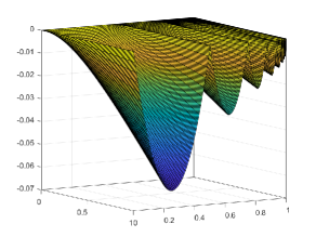
Figure 1. $M(x,y)$

This shows that $\mathcal{I}^{\gamma}M(x,y)$ is finite on $[0,1]\times[0,1]$. Since $M(x,y)$ is a continuous function and of bounded variation on $[0,1)\times[0,1),$ then from Lemma 6.2 we know that $\mathcal{I}^{\gamma}M(x,y)$ is continuous and of bounded variation on $[0,1)\times[0,1)$ for $0<\gamma_{1}<1,~{}0<\gamma_{2}<1$.
Let $0<\delta<1$ and a positive constant $C$, when $(x,y)\in[0,1-\delta)\times[0,1-\delta),$ $\mathcal{I}^{\gamma}M(x,y)$ is of bounded variation. Let the smallest number of sets of diameter $\delta$ which can cover graph of $\mathcal{I}^{\gamma}M(x,y)$ is $\frac{C}{\delta^{2}}.$ Now, when $(x,y)\in[1,1-\delta)\times[1,1-\delta),$ then the number of $\delta$-cubes that intersect graph of $\mathcal{I}^{\gamma}M(x,y)$ is at most $\frac{1}{\delta^{2}}.$
Hence, the smallest number of sets of diameter $\delta$ which can cover graph of $\mathcal{I}^{\gamma}M(x,y)$ is at most $\frac{C+1}{\delta^{2}}.$ Thus, we have

$$\overline{\dim}_{B}Gr(\mathcal{I}^{\gamma}M,[0,1]\times[0,1])=\overline{\lim_{\delta\to 0}}\frac{\log N_{\delta}(Gr(\mathcal{I}^{\gamma}M))}{-\log\delta}\leq\lim_{\delta\to 0}\frac{\log\frac{C+1}{\delta^{2}}}{-\log\delta}=2.$$

From Definition 2.2 and Lemma 5.1, we know that

$$\underline{\dim}_{B}Gr(\mathcal{I}^{\gamma}M,[0,1]\times[0,1])\geq 2.$$

This implies that

(6.1) $$\dim_{B}Gr(\mathcal{I}^{\gamma}M,[0,1]\times[0,1])=2.$$

Also, we know that

(6.2) $$2\leq\dim_{H}Gr(\mathcal{I}^{\gamma}M,[0,1]\times[0,1])\leq\dim_{B}Gr(\mathcal{I}^{\gamma}M,[0,1]\times[0,1]).$$

From Equations 6.1 and 6.2, we get the required result. ∎

Remark 6.3.

From [20], we know that if a function is continuous and of bounded variation in Arzelá sense, then its fractional integral of mixed R-L type is also continuous and of bounded variation in Arzelá sense and its fractal dimension is 2. From Theorem 6.2, we conclude that the box dimension and the Hausdorff dimension of the fractional integral of mixed R-L type of unbounded variational continuous function are also 2. So, $M$ is the such example which is of unbounded variational continuous function but the fractal dimension of its the fractional integral of mixed R-L type is 2.

Acknowledgements

First author has received the financial supported from the CSIR, India (file no: 09/1058(0012)/2018-EMR-I).

References

- [1] C. R. Adams and J. A. Clarkson, Properties of functions of bounded variation, Trans. Amer. Math. Soc. 36(4) (1934) 711-730.
- [2] M. F. Barnsley, Fractal Everywhere, Academic Press, Orlando, Florida, 1988.
- [3] K. Barański, B. Bárány, J. Romanowska, On the dimension of the graph of the classical Weierstrass function, Adv. Math. 265 (2014) 32–59.
- [4] J. A. Clarkson, C. R. Adams, On definitions of bounded variation for functions of two variables, Trans. Amer. Math. Soc. 35 (1933) 824-854.
- [5] S. Chandra and S. Abbas, The calculus of bivariate fractal interpolation surfaces, Fractals 29(4) (2021) 2150066.
- [6] J. Falconer, Fractal Geometry: Mathematical Foundations and Applications, John Wiley Sons Inc., New York, 1999.
- [7] Z. Feng, Variation and Minkowski dimension of fractal interpolation surface, J. Math. Anal. Appl. 345 (1)(2008)322-334.
- [8] Z. Feng, X. Sun, Box-counting dimensions of fractal interpolation surfaces derived from fractal interpolation functions, J. Math. Anal. Appl., 412 (1) (2014) 416-425.
- [9] B.R. Hunt, The Hausdorff dimension of graphs of Weierstrass functions, Proc. Am. Math. Soc. 126(3) (1998) 791–800.
- [10] Y. S. Liang, Box dimensions of Riemann-Liouville fractional integrals of continuous functions of bounded variation, Nonlin. Anal. 72 (2010) 4304-4306.
- [11] Y. S. Liang, Fractal dimension of Riemann-Liouville fractional integral of 1-dimensional continuous functions, Fractional Calculus and Applied Analysis, 21(6) 2019 1651-1658.
- [12] W. Shen, Hausdorff dimension of the graphs of the classical Weierstrass functions, Math. Z. 289(1–2) (2018) 223–266.
- [13] S. G. Samko, A. A. Kilbas, O. I. Marichev, Fractional Integrals and Derivatives, Theory and Applications, Gordon and Breach, Yverdon et alibi, (1993).
- [14] A. A. Kilbas, H. M. Srivastava and J. J. Trujillo, Theory and Applications of Fractional Differential Equations, Elsevier B. V. Amsterdam, Netherlands 2006.
- [15] I. Podlubny, Fractional Differential Equations, Academic Press, San Diego, California-USA 1999.
- [16] H. J. Ruan, W. Y. Su and K. Yao, Box dimension and fractional integral of linear fractal interpolation functions, Journal of Approximation Theory, 161 (2009) 187-197.
- [17] F. B. Tatom, The relationship between fractional calculus and fractals, Fractals 3 (1995) 217-229.
- [18] J. R. Wu, The effects of the Riemann-Liouville fractional integral on the box dimension of fractal graphs of Hölder continuous functions, Fractals 28 (2020) 2050052-1304.
- [19] J. R. Wu, On a linearity between fractal dimension and order of fractional calculus in Hölder space, Appl. Math. Comput. 385 (2020) 125433.
- [20] S. Verma, P. Viswanathan, Bivariate functions of bounded variation: Fractal dimension and fractional integral, Indag. Math. (2020) 294-309.
- [21] S. Verma, Some Results on Fractal Functions, Fractal Dimensions and Fractional Calculus, Ph.D. thesis, Indian Institute of Technology Delhi, India, 2020.
- [22] S. Verma, Y. S. Liang, Effect of the Riemann-Liouville fractional integral on unbounded variation points, arXiv preprint arXiv:2008.11113 (2020).
- [23] K. Yao, W. Y. Su and S. P. Zhou, On the connection between the order of the fractional calculus and the dimension of a fractal function, Chaos, Solitons and Fractals, 23 (2005) 621-629.