Monash Time Series Forecasting Archive

Abstract

Many businesses and industries nowadays rely on large quantities of time series data making time series forecasting an important research area. Global forecasting models that are trained across sets of time series have shown a huge potential in providing accurate forecasts compared with the traditional univariate forecasting models that work on isolated series. However, there are currently no comprehensive time series archives for forecasting that contain datasets of time series from similar sources available for the research community to evaluate the performance of new global forecasting algorithms over a wide variety of datasets. In this paper, we present such a comprehensive time series forecasting archive containing 20 publicly available time series datasets from varied domains, with different characteristics in terms of frequency, series lengths, and inclusion of missing values. We also characterise the datasets, and identify similarities and differences among them, by conducting a feature analysis. Furthermore, we present the performance of a set of standard baseline forecasting methods over all datasets across eight error metrics, for the benefit of researchers using the archive to benchmark their forecasting algorithms.

1 Introduction

Accurate time series forecasting is important for many businesses and industries to make decisions, and consequently, time series forecasting is a popular research area, lately in particular in machine learning. A good benchmarking archive is essential for the growth of machine learning research [103]. Researchers gain the opportunity to perform a rigorous evaluation of their newly proposed machine learning algorithms over a large number of datasets when there is a proper benchmarking archive available. The University of California Irvine (UCI) repository [28] is the most common and well-known benchmarking archive used in general machine learning, and it has supported the development of many state-of-the-art algorithms. The UCI repository currently contains 507 datasets from various domains.

In time series classification, there exist two well-known publicly available dataset archives: University of California Riverside (UCR) repository [26] and University of East Anglia (UEA) repository [9]. The UCR repository was first released in 2002 with 16 datasets and at present, the number of datasets is 128, containing datasets of non-normalised time series, of varying lengths, and time series with missing values [26]. The UCR repository contains only univariate time series datasets. Therefore, recently a group of researchers from UEA released the first multivariate time series classification archive which is known as UEA repository [9]. Currently, it contains 30 datasets containing equal length multivariate time series without any missing values. Furthermore, Tan et al. [103] recently released the first time series extrinsic regression archive containing 19 multi-dimensional time series datasets.

On the other hand, there are many time series forecasting competitions which have advanced the field. The most popular forecasting competition series is the M-competition series [71, 72, 73, 74]. The latest competition of this series was the M5 competition [75] which is the fifth iteration of the series, and finished in July 2020. Other well-known forecasting competitions include the NN3 and NN5 Neural Network competitions [15], the CIF 2016 competition [100], and Kaggle competitions such as the Wikipedia web traffic [42] and Rossmann sales forecasting [60] competitions. The winning approaches of many of these competitions such as the winning method of the M4 forecasting by Smyl [95] and the winning method of the M5 forecasting competition based on gradient boosted trees, consist of global forecasting models [57] which train a single model across all series that need to be forecast. Compared with local models, global forecasting models have the ability to learn cross-series information during model training and can control model complexity and overfitting on a global level [81]. By now, many works have shown the superior performance of global models over per-series models in many situations [11, 45, 81, 32, 108, 40, 39, 41].

This can be seen as a paradigm shift in forecasting. Over decades, single time series were seen as a dataset that should be studied and modelled in isolation. Nowadays, we are oftentimes interested in global models built on sets of series from similar sources, such as series which are all product sales from a particular store, or series which are all smart meter readings in a particular city or state. Here, time series are seen as an instance in a dataset of many time series, to be studied and modelled together.

Though in the time series forecasting space there are a number of benchmarking archives, they follow the paradigm of single series as datasets, and consequently contain mostly unrelated single time series such as the Time Series Data Library [52], ForeDeCk [33], the datasets of the M3 and M4 forecasting competitions, and others. These archives are of limited use to evaluate the performance of global forecasting models that typically are designed for, and perform better on, sets of series from similar sources (a notable exception from the rule being here ES-RNN by Smyl [95], the winning method of the M4 competition). There are currently no comprehensive time series forecasting benchmarking archives, to the best of our knowledge, that focus on such datasets of related time series to evaluate the performance of such global forecasting algorithms. Our aim is to address this limitation by introducing such an archive. In particular, our paper has the following main contributions.

• We introduce the first comprehensive time series forecasting archive containing datasets of related time series, available at https://forecastingdata.org/. This archive contains 20 publicly available time series datasets, with both equal and variable lengths time series. Many datasets have different versions based on the frequency and the inclusion of missing values, making the total number of dataset variations to 50. Furthermore, it includes both real-world and competition time series datasets covering varied domains.

• We introduce a new format to store time series data, based on the Weka ARFF file format [85] and overcoming some of the shortcomings we observe in the .ts format used in the sktime time series repository [67]. We use a .tsf extension for this new format. This format stores the meta-information about a particular time series dataset such as dataset name, frequency and inclusion of missing values as well as the series specific information such as starting timestamps, in a non-redundant way. The format is very flexible and capable of including any other attributes related to time series as preferred by the users.

• We analyse the characteristics of different series to identify the similarities and differences among them. For that, we conduct a feature analysis using tsfeatures [50] and catch22 features [69] extracted from all series of all datasets. The extracted features are publicly available for further research use.

• We evaluate the performance of a set of baseline forecasting models including both traditional univariate forecasting models and global forecasting models over all datasets across eight error metrics. The forecasts and evaluation results of the baseline methods are publicly available for the benefits of researchers that use the repository to benchmark their forecasting algorithms.

• Finally, all implementations related to the forecasting archive including code for loading the datasets into the R and Python environments and code for feature calculations and evaluation of baseline forecasting models are publicly available at: https://github.com/rakshitha123/TSForecasting.

We also encourage other researchers to contribute time series datasets to our repository either by directly uploading them into the archive and/or by contacting the authors via email. The remainder of this paper is organised as follows: Section 2 explains the datasets in the archive. Section 3 explains the details of the feature analysis. Section 4 presents results of the baseline forecasting models over the datasets across eight error metrics. Finally, Section 5 concludes the paper.

2 Datasets

This section details the datasets in our time series forecasting archive. The current archive contains 20 time series datasets. Furthermore, the archive contains in addition 6 single very long time series. As a large amount of data oftentimes renders machine learning methods feasible compared with traditional statistical modelling, and we are not aware of good and systematic benchmark data in this space either, these series are included in our repository as well. A summary of all primary datasets included in the repository is shown in Table 1.

A total of 50 datasets have been derived from these 26 primary datasets. Nine datasets contain time series belonging to different frequencies and the archive contains a separate dataset per each frequency. Seven of the datasets have series with missing values. The archive contains 2 versions of each of these, one with and one without missing values. In the latter case, the missing values have been replaced by using an appropriate imputation technique.

	Dataset	Domain	No: of	Min.	Max.	No: of	Missing	Competition
			Series	Length	Length	Freq.
1	M1	Multiple	1001	15	150	3	No	Yes
2	M3	Multiple	3003	20	144	4	No	Yes
3	M4	Multiple	100000	19	9933	6	No	Yes
4	Tourism	Tourism	1311	11	333	3	No	Yes
5	NN5	Banking	111	791	791	2	Yes	Yes
6	CIF 2016	Banking	72	34	120	1	No	Yes
7	Web Traffic	Web	145063	803	803	2	Yes	Yes
8	Solar	Energy	137	52560	52560	2	No	No
9	Electricity	Energy	321	26304	26304	2	No	No
10	London Smart Meters	Energy	5560	288	39648	1	Yes	No
11	Wind Farms	Energy	339	6345	527040	1	Yes	No
12	Car Parts	Sales	2674	51	51	1	Yes	No
13	Dominick	Sales	115704	28	393	1	No	No
14	FRED-MD	Economic	107	728	728	1	No	No
15	San Francisco Traffic	Transport	862	17544	17544	2	No	No
16	Pedestrian Counts	Transport	66	576	96424	1	No	No
17	Hospital	Health	767	84	84	1	No	No
18	COVID Deaths	Nature	266	212	212	1	No	No
19	KDD Cup	Nature	270	9504	10920	1	Yes	Yes
20	Weather	Nature	3010	1332	65981	1	No	No
21	Sunspot	Nature	1	73931	73931	1	Yes	No
22	Saugeen River Flow	Nature	1	23741	23741	1	No	No
23	US Births	Nature	1	7305	7305	1	No	No
24	Electricity Demand	Energy	1	17520	17520	1	No	No
25	Solar Power	Energy	1	7397222	7397222	1	No	No
26	Wind Power	Energy	1	7397147	7397147	1	No	No

Table 1: Datasets in the Current Time Series Forecasting Archive

Out of the 26 datasets, 8 originate from competition platforms, 3 from Lai et al. [65], 6 are taken from R packages, 1 is from the Kaggle platform [61], and 1 is taken from a Johns Hopkins repository [24]. The other datasets have been extracted from corresponding domain specific platforms. The datasets mainly belong to 9 different domains: tourism, banking, web, energy, sales, economics, transportation, health, and nature. Three datasets, the M1 [71], M3 [72], and M4 [73, 74] datasets, contain series belonging to multiple domains.

For all datasets, we introduce their key characteristics as well as the citations of the prior work where they have been used in the literature. Further details of these datasets are explained in the next sections, after describing the data format in which the series are stored.

2.1 Data Format

We also introduce a new format to store time series data, based on the Weka ARFF file format [85]. We use the file extension .tsf and it is comparable with the .ts format used in the sktime time series repository [67], but we deem it more streamlined and more flexible. The basic idea of the file format is that each data file can contain 1) attributes that are constant throughout the whole dataset (e.g., the forecasting horizon, whether the dataset contains missing values or not), 2) attributes that are constant throughout a time series (e.g., its name, its position in a hierarchy, product information for product sales time series), and 3) attributes that are particular to each data point (the value of the series, or timestamps for non-equally spaced series). An example of series in this format is shown in Figure 1.

Figure 1: An example of the file format for the NN5 daily dataset

The original Weka ARFF file format already deals well with the first two types of such attributes. Using this file format, in our format, each time series file contains tags describing the meta-information of the corresponding dataset such as @frequency (seasonality), @horizon (expected forecast horizon), @missing (whether the series contain missing values) and @equallength (whether the series have equal lengths). We note that these attributes can be freely defined by the user and the file format does not need any of these values to be defined in a certain way, though the file readers reading the files may rely on existence of attributes with certain names and assume certain meanings. Next, there are attributes in each dataset which describe series-wise properties, where the tag @attribute is followed by the name and type. Examples are series_name (the unique identifier of a given series) and start_ timestamp (the start timestamp of a given series). Again, the format has the flexibility to include any additional series-wise attributes as preferred by users.

Following the ARFF file format, the data are then listed under the @data tag after defining attributes and meta-headers, and attribute values are separated by colons. The only extension that our format has compared with the original ARFF file format, is that the time series then are appended to their attribute vector as a comma-separated variable-length vector. As this vector can have a different length for each instance, this cannot be represented in the original ARFF file format. In particular, a time series with $m$ number of attributes and $n$ number of values can be shown as:

$$<attribute_{1}>:<attribute_{2}>:...:<attribute_{m}>:<s_{1},s_{2},...,s_{n}>$$ (1)

The missing values in the series are indicated using the “?” symbol. Code to load datasets in this format into R and Python is available in our github repository.

2.2 Time Series Datasets

This section describes the benchmark datasets that have a sufficient number of series from a particular frequency. The datasets may contain different categories in terms of domain and frequency.

2.2.1 M1 Dataset

The M1 competition dataset [71] contains 1001 time series with 3 different frequencies: yearly, quarterly, and monthly as shown in Table 2. The series belong to 7 different domains: macro 1, macro 2, micro 1, micro 2, micro 3, industry, and demographic.

Frequency	No: of Series	Min. Length	Max. Length	Forecast Horizon
Yearly	181	15	58	6
Quarterly	203	18	114	8
Monthly	617	48	150	18
Total	1001

Table 2: Summary of M1 Dataset

Research work which uses this dataset includes:

• Forecasting with artificial neural networks: the state of the art [114]

• Time series forecasting using a hybrid ARIMA and neural network model [113]

• Automatic time series forecasting: the forecast package for R [51]

• Exponential Smoothing: the state of the art [37]

• Neural network forecasting for seasonal and trend time series [115]

2.2.2 M3 Dataset

The M3 competition dataset [72] contains 3003 time series of various frequencies including yearly, quarterly, and monthly, as shown in Table 3. The series belong to 6 different domains: demographic, micro, macro, industry, finance, and other.

Frequency	No: of Series	Min. Length	Max. Length	Forecast Horizon
Yearly	645	20	47	6
Quarterly	756	24	72	8
Monthly	1428	66	144	18
Other	174	71	104	8
Total	3003

Table 3: Summary of M3 Dataset

Research work which uses this dataset includes:

• The theta model: a decomposition approach to forecasting [7]

• Recurrent neural networks for time series forecasting: current status and future directions [45]

• Out-of-sample tests of forecasting accuracy: an analysis and review [104]

• Metrics for evaluating performance of prognostic techniques [93]

• Temporal link prediction using matrix and tensor factorizations [29]

• Forecasting time series with complex seasonal patterns using exponential smoothing [66]

• Evaluating forecasting methods [6]

• Exponential smoothing with a damped multiplicative trend [105]

2.2.3 M4 Dataset

The M4 competition dataset [73, 74] contains 100,000 time series with 6 different frequencies: yearly, quarterly, monthly, weekly, daily, and hourly, as shown in Table 4. The series belong to 6 different domains: demographic, micro, macro, industry, finance, and other, similar to the M3 forecasting competition. This dataset contains a subset of series available at ForeDeCk [33].

Frequency	No: of Series	Min. Length	Max. Length	Forecast Horizon
Yearly	23000	19	841	6
Quarterly	24000	24	874	8
Monthly	48000	60	2812	18
Weekly	359	93	2610	13
Daily	4227	107	9933	14
Hourly	414	748	1008	48
Total	100000

Table 4: Summary of M4 Dataset

Research work which uses this dataset includes:

• A hybrid method of exponential smoothing and recurrent neural networks for time series forecasting [95]

• FFORMA: Feature-based Forecast Model Averaging [80]

• Recurrent neural networks for time series forecasting: current status and future directions [45]

• LSTM-MSNet: leveraging forecasts on sets of related time series with multiple seasonal patterns [10]

• Are forecasting competitions data representative of the reality? [99]

• Averaging probability forecasts: back to the future [112]

• A strong baseline for weekly time series forecasting [40]

2.2.4 Tourism Dataset

This dataset originates from a Kaggle competition [8, 31] and contains 1311 tourism related time series with 3 different frequencies: yearly, quarterly, and monthly as shown in Table 5.

Frequency	No: of Series	Min. Length	Max. Length	Forecast Horizon
Yearly	518	11	47	4
Quarterly	427	30	130	8
Monthly	366	91	333	24
Total	1311

Table 5: Summary of Tourism Dataset

Research work which uses this dataset includes:

• Recurrent neural networks for time series forecasting: current status and future directions [45]

• A meta-analysis of international tourism demand forecasting and implications for practice [87]

• Improving forecasting by estimating time series structural components across multiple frequencies [64]

• Forecasting tourist arrivals using time-varying parameter structural time series models [97]

• Forecasting monthly and quarterly time series using STL decomposition [106]

• A novel approach to model selection in tourism demand modeling [3]

2.2.5 NN5 Dataset

This dataset contains 111 time series of daily cash withdrawals from Automated Teller Machines (ATM) in the UK, and was used in the NN5 forecasting competition [15]. The forecast horizon considered in the competition was 56. The original dataset contains missing values. Our repository contains two versions of the dataset: the original version with missing values and a modified version where the missing values have been replaced using a median substitution where a missing value on a particular day is replaced by the median across all the same days of the week along the whole series as in Hewamalage et al. [45]. Furthermore, Godahewa et al. [40] use the weekly aggregated version of this dataset for their experiments related to proposing a baseline model for weekly forecasting. The aggregated weekly version of this dataset is also available in our repository. Research work which uses this dataset includes:

• Recurrent neural networks for time series forecasting: current status and future directions [45]

• A strong baseline for weekly time series forecasting [40]

• Forecasting across time series databases using recurrent neural networks on groups of similar series: a clustering approach [11]

• Forecast combinations of computational intelligence and linear models for the NN5 time series forecasting competition [5]

• Forecasting the NN5 time series with hybrid models [111]

• Multiple-output modeling for multi-step-ahead time series forecasting [16]

• Recursive multi-step time Series forecasting by perturbing data [14]

• Benchmarking of classical and machine-learning algorithms (with special emphasis on bagging and boosting approaches) for time series forecasting [90]

2.2.6 CIF 2016 Dataset

The dataset from the Computational Intelligence in Forecasting (CIF) 2016 forecasting competition contains 72 monthly time series. Out of those, 24 series originate from the banking sector, and the remaining 48 series are artificially generated. There are 2 forecast horizons considered in the competition where 57 series have a forecasting horizon of 12 and the remaining 15 series consider the forecast horizon as 6 [100]. Research work which uses this dataset includes:

• Recurrent neural networks for time series forecasting: current status and future directions [45]

• Forecasting across time series databases using recurrent neural networks on groups of similar series: a clustering approach [11]

• Improving time series forecasting: an approach combining bootstrap aggregation, clusters and exponential smoothing [25]

• Time series clustering using numerical and fuzzy representations [2]

• An automatic calibration framework applied on a metaheuristic fuzzy model for the CIF competition [23]

2.2.7 Kaggle Web Traffic Dataset

This dataset contains 145063 daily time series representing the number of hits or web traffic for a set of Wikipedia pages from 01/07/2015 to 10/09/2017 used by the Kaggle web traffic forecasting competition [42]. The forecast horizon considered in the competition was 59. As the original dataset contains missing values, we include both the original dataset in our repository and an imputed version. This dataset is intermittent and hence, we impute missing values with zeros. Furthermore, Godahewa et al. [40] use the weekly aggregated version of this dataset containing the first 1000 series. Our repository also contains this aggregated weekly version of the dataset for all series. The missing values of the original dataset were imputed before the aggregation. Research work which uses this dataset includes:

• Recurrent neural networks for time series forecasting: current status and future directions [45]

• A strong baseline for weekly time series forecasting [40]

• Web traffic prediction of Wikipedia pages [88]

• Improving time series forecasting using mathematical and deep learning models [44]

• Foundations of sequence-to-sequence modeling for time series [77]

2.2.8 Solar Dataset

This dataset contains 137 time series representing the solar power production recorded every 10 minutes in the state of Alabama in 2006. It was used by Lai et al. [65], and originally extracted from Solar [96]. Furthermore, Godahewa et al. [40] use an aggregated version of this dataset containing weekly solar power production records. The aggregated weekly version of this dataset is also available in our repository.

2.2.9 Electricity Dataset

This dataset represents the hourly electricity consumption of 321 clients from 2012 to 2014 in kilowatt (kW). It was used by Lai et al. [65], and originally extracted from UCI [109]. Our repository also contains an aggregated version of this dataset representing the weekly electricity consumption values.

2.2.10 London Smart Meters Dataset

This dataset contains 5560 half-hourly time series that represent the energy consumption readings of London households in kWh from November 2011 to February 2014 [58]. The series are categorized into 112 blocks in the original dataset. The series in our repository are in the same order (from block 0 to block 111) as they are in the original dataset. The original dataset contains missing values and we impute them using the last observation carried forward (LOCF) method. Our repository contains both versions: the original version with missing values and the modified version where the missing values have been replaced. Research work which uses this dataset includes:

• Predicting electricity consumption using deep Recurrent Neural Networks [82]

• A single scalable LSTM model for short-term forecasting of disaggregated electricity loads [4]

• Deep learning based short-term load forecasting for urban areas [76]

• Smart grid energy management using RNN-LSTM: a deep learning-based approach [62]

2.2.11 Wind Farms Dataset

This dataset contains very long minutely time series representing the wind power production of 339 wind farms in Australia. It was extracted from the Australian Energy Market Operator (AEMO) online platform [1]. The series in this dataset range from 01/08/2019 to 31/07/2020. The original dataset contains missing values where some series contain missing data for more than seven consecutive days. Our repository contains both the original version of the dataset and a version where the missing values have been replaced by zeros.

2.2.12 Car Parts Dataset

This dataset contains 2674 intermittent monthly time series showing car parts sales from January 1998 to March 2002. It was extracted from the R package expsmooth [48]. The package contains this dataset as “carparts”. As the original dataset contains missing values, we include the original version of the dataset in the repository as well as a version where the missing values have been replaced with zeros, as the series are intermittent. Research work which uses this dataset includes:

• Principles and algorithms for forecasting groups of time series: locality and globality [81]

2.2.13 Dominick Dataset

This dataset contains 115704 weekly time series representing the profit of individual stock keeping units (SKU) from a retailer.

It was extracted from the Kilts Center, University of Chicago Booth School of Business online platform [55]. This platform also contains daily store-level sales data on more than 3500 products collected from Dominick’s Finer Foods, a large American retail chain in the Chicago area, for approximately 9 years. The data are provided in different categories such as customer counts, store-specific demographics and sales products. Research work which uses this dataset includes:

• Principles and algorithms for forecasting groups of time series: locality and globality [81]

• The value of competitive information in forecasting FMCG retail product sales and the variable selection problem [46]

• Beer snobs do exist: estimation of beer demand by type [107]

• Downsizing and supersizing: how changes in product attributes influence consumer preferences [56]

• Reference prices, costs, and nominal rigidities [30]

• Sales and monetary policy [43]

2.2.14 FRED-MD Dataset

This dataset contains 107 monthly time series showing a set of macro-economic indicators from the Federal Reserve Bank [78] starting from 01/01/1959. It was extracted from the FRED-MD database. The series are differenced and log-transformed as suggested in the literature. Research work which uses this dataset includes:

• Principles and algorithms for forecasting groups of time series: locality and globality [81]

2.2.15 San Francisco Traffic Dataset

This dataset contains 862 hourly time series showing the road occupancy rates on San Francisco Bay area freeways from 2015 to 2016. It was used by Lai et al. [65], and originally extracted from [20]. Godahewa et al. [40] use a weekly aggregated version of this dataset, which is also available in our repository.

2.2.16 Melbourne Pedestrian Counts Dataset

This dataset contains hourly pedestrian counts captured from 66 sensors in Melbourne city starting from May 2009 [22]. The original data are updated on a monthly basis when the new observations become available. The dataset in our repository contains pedestrian counts up to 30/04/2020. Research work which uses this dataset includes:

• Enhancing pedestrian mobility in smart cities using big data [21]

• Visualising Melbourne pedestrian count [83]

• PedaViz: visualising hour-level pedestrian activity [84]

2.2.17 Hospital Dataset

This dataset contains 767 monthly time series showing the patient counts related to medical products from January 2000 to December 2006. It was extracted from the R package expsmooth [48]. The package contains this dataset as “hospital”. Research work which uses this dataset includes:

• Principles and algorithms for forecasting groups of time series: locality and globality [81]

2.2.18 COVID Deaths Dataset

This dataset contains 266 daily time series that represent the total COVID-19 deaths in a set of countries and states from 22/01/2020 to 20/08/2020. It was extracted from the Johns Hopkins repository [24, 27]. The original data are updated on a daily basis when the new observations become available.

2.2.19 KDD Cup 2018 Dataset

This competition dataset contains long hourly time series representing the air quality levels in 59 stations in 2 cities, Beijing (35 stations) and London (24 stations) from 01/01/2017 to 31/03/2018 [63]. The dataset represents the air quality in multiple measurements such as $PM2.5$, $PM10$, $NO_{2}$, $CO$, $O_{3}$ and $SO_{2}$ levels.

Our repository dataset contains 270 hourly time series which have been categorized using city, station name, and air quality measurement.

As the original dataset contains missing values, we include both the original dataset and an imputed version in our repository. We impute leading missing values with zeros and the remaining missing values using the LOCF method. Research work which uses this dataset includes:

• AccuAir: winning solution to air quality prediction for KDD cup 2018 [70]

2.2.20 Weather Dataset

This dataset contains 3010 daily time series representing the variations of four weather variables: rain, minimum temperature, maximum temperature and solar radiation, measured at weather stations in Australia. The series were extracted from the R package bomrang [98]. Research work which uses this dataset includes:

• Principles and algorithms for forecasting groups of time series: locality and globality [81]

2.3 Single Long Time Series Datasets

This section describes the benchmark datasets which have single time series with a large amount of data points.

2.3.1 Sunspot Dataset

The original data source contains a single very long daily time series of sunspot numbers from 01/01/1818 until the present [102]. Furthermore, it also contains monthly mean total sunspot numbers (starting from 1749), 13-month smoothed monthly total sunspot numbers (starting from 1749), yearly mean total sunspot numbers (starting from 1700), daily hemispheric sunspot numbers (starting from 1992), monthly mean hemispheric sunspot numbers (starting from 1992), 13-month smoothed monthly hemispheric sunspot numbers (starting from 1992), and yearly mean total sunspot numbers (starting from 1610). The original datasets are updated as new observations become available.

Our repository contains the single daily time series representing the sunspot numbers from 08/01/1818 to 31/05/2020. As the dataset contains missing values, we include an LOCF-imputed version besides it in the repository. Research work which uses this dataset includes:

• Re-evaluation of predictive models in light of new data: sunspot number version 2.0 [38]

• Correlation between sunspot number and ca II K emission index [17]

• Dynamics of sunspot series on time scales from days to years: correlation of sunspot births, variable lifetimes, and evolution of the high-frequency spectral component [94]

• Long term sunspot cycle phase coherence with periodic phase disruptions [86]

2.3.2 Saugeen River Flow Dataset

This dataset contains a single very long time series representing the daily mean flow of the Saugeen River at Walkerton in cubic meters per second from 01/01/1915 to 31/12/1979. The length of this time series is 23,741. It was extracted from the R package, deseasonalize [79]. The package contains this dataset as “SaugeenDay”.

Research work which uses this dataset includes:

• Telescope: an automatic feature extraction and transformation approach for time series forecasting on a level-playing field [12]

2.3.3 US Births Dataset

This dataset contains a single very long daily time series representing the number of births in the US from 01/01/1969 to 31/12/1988. The length of this time series is 7,305. It was extracted from the R package, mosaicData [91]. The package contains this dataset as “Births”. Research work which uses this dataset includes:

• Telescope: an automatic feature extraction and transformation approach for time series forecasting on a level-playing field [12]

2.3.4 Electricity Demand Dataset

This dataset contains a single very long time series representing the half hourly electricity demand for Victoria, Australia in 2014. The length of this time series is 17,520. It was extracted from the R package, fpp2 [49]. The package contains this dataset as “elecdemand”. The temperatures corresponding with each demand value are also available in the original dataset. Research work which uses this dataset includes:

• Telescope: an automatic feature extraction and transformation approach for time series forecasting on a level-playing field [12]

2.3.5 Solar Power Dataset

This dataset contains a single very long time series representing the solar power production of an Australian wind farm recorded per each 4 seconds starting from 01/08/2019. It was extracted from the AEMO online platform [1]. The length of this time series is 7,397,222.

2.3.6 Wind Power Dataset

This dataset contains a single very long time series representing the wind power production of an Australian wind farm recorded per each 4 seconds starting from 01/08/2019. It was extracted from the AEMO online platform [1]. The length of this time series is 7,397,147.

3 Feature Analysis

We characterise the datasets in our archive to analyse the similarities and differences between them, to gain a better understanding on where gaps in the repository may be and what type of data are prevalent in real-world applications. This may also help to select suitable forecasting methods for different types of datasets. We analyse the characteristics of the datasets using the tsfeatures [50] and catch22 [69] feature extraction methods. All extracted features are publicly available for further research use. Due to their large size, we have not been able to extract features from the London smart meters, wind farms, solar power, and wind power datasets, which is why we exclude them from this analysis.

We extract 42 features using the tsfeatures function in the R package tsfeatures [50] including mean, variance, autocorrelation features, seasonal features, entropy, crossing points, flat spots, lumpiness, non-linearity, stability, Holt-parameters, and features related to the Kwiatkowski–Phillips–Schmidt–Shin (KPSS) test [13] and the Phillips–Perron (PP) test [89]. For all series that have a frequencies greater than daily, we consider multi-seasonal frequencies when computing features. Therefore, the amount of features extracted is higher for multi-seasonal datasets as the seasonal features are individually calculated for each season presented in the series. Furthermore, if a series is short and does not contain two full seasonal cycles, we calculate the features assuming a non-seasonal series (i.e., setting its frequency to “one” for the feature extraction). We use the catch22_all function in the R package catch22 [68] to extract the catch22 features from a given time series. The features are a subset of 22 features from the hctsa package [36] which includes the implementations of over 7000 time series features. The computational cost of the catch22 features is low compared with all features implementated in the hctsa package.

In the following feature analysis, we consider 5 features, as suggested by Bojer and Meldgaard [18]: first order autocorrelation (ACF1), trend, entropy, seasonal strength, and the Box-Cox transformation parameter, lambda. The BoxCox.lambda function in the R package forecast [51] is used to extract the Box-Cox transformation parameter from each series, with default parameters. The other 4 features are extracted using tsfeatures. Since this feature space contains 5 dimensions, to compare and visualise the features across multiple datasets, we reduce the feature dimensionality to 2 using Principal Component Analysis [PCA, 59].

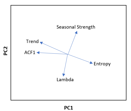
Figure 2: The directions of the 5 feature components: ACF1, trend, entropy, seasonal strength, and lambda, for the two-dimensional feature space generated by the first two principal components (PC1, PC2) extracted with PCA.

The numbers of series in each dataset are significantly different, e.g., the CIF 2016 monthly dataset and M4 monthly dataset contain 72 and 48,000 series, respectively. Hence, if all series were considered to calculate the PCA components, those components would be dominated by datasets that have large amounts of series. Therefore, for datasets that contain more than 300 series, we randomly take a sample of 300 series, before constructing the PCA components across all datasets. Once the components are calculated, we map all series of all datasets into the resulting PCA feature space. We note that we use PCA for dimensionality reduction over other advanced dimensionality reduction algorithms such as t-Distributed Stochastic Neighbor Embedding [t-SNE, 110] due to this capability of constructing the basis of the feature space with a reduced sample of series with the possibility to then map all series into the space afterwards. The directions of the 5 corresponding feature components generated by PCA are shown in Figure 2.

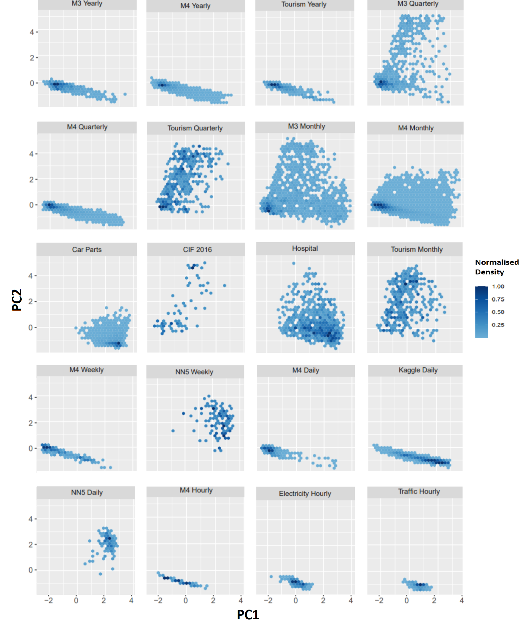
Figure 3: Hexbin plots showing the normalised density values of the low-dimensional feature space generated by PCA across ACF1, trend, entropy, seasonal strength and lambda for 20 datasets. The dark and light hexbins denote the high and low density areas, respectively.

Figure 3 accordingly shows hexbin plots of the normalised density values for 20 datasets. The figure highlights the characteristics among different datasets. For the M competition datasets, the feature space is highly populated on the left-hand side and hence, denoting high trend and ACF1 levels in the series. The tourism yearly dataset also shows high trend and ACF1 levels. In contrast, the car parts, hospital, and Kaggle web traffic datasets show high density levels towards the right-hand side, indicating a higher degree of entropy. The presence of intermittent series can be considered the major reason for the higher degree of entropy in the Kaggle web traffic and car parts datasets. The plots confirm the claim by Bojer and Meldgaard [18] and Fry and Brundage [35] that the M competition datasets are significantly different from the Kaggle web traffic dataset.

The monthly datasets generally show high seasonal strengths compared with datasets of other frequencies. Quarterly datasets also demonstrate high seasonal strengths except for the M4 quarterly dataset. In contrast, the datasets with high frequencies such as weekly, daily, and hourly show low seasonal strengths except for the NN5 weekly and NN5 daily datasets.

Related to the shapes of the feature space, the 3 yearly datasets: M3, M4, and tourism show very similar shapes and density populations indicating they have similar characteristics. The M4 quarterly dataset also shows a similar shape as the yearly datasets, even though it has a different frequency. The other 2 quarterly datasets M3 and tourism are different, but similar to each other. The M3 and M4 monthly datasets are similar to each other in terms of both shape and density population. Furthermore, the electricity hourly and traffic hourly datasets have similar shapes and density populations, whereas the M4 hourly dataset has a slightly different shape compared with them. The daily datasets show different shapes and density populations, where the NN5 daily dataset is considerably different from the other 2 daily datasets: M4 and Kaggle web traffic, in terms of shape and all 3 daily datasets are considerably different from each other in terms of density population. The weekly datasets also show different shapes and density populations compared with each other.

PCA plots showing the normalized density values of all datasets corresponding with both tsfeatures and catch22 features are available in the Online Appendix.

4 Baseline Forecasting Models

In this section, we evaluate the performance of different baseline forecasting models including 6 traditional univariate forecasting models and a global forecasting model over the datasets in our repository using a fixed origin evaluation scheme, so that researchers that use the data in our repository can directly benchmark their forecasting algorithms against these baselines. The following 7 baseline forecasting methods are considered for the experiments:

• Exponential Smoothing [ETS, 47]

• Auto-Regressive Integrated Moving Average [ARIMA, 19]

• Simple Exponential Smoothing (SES)

• Theta [7]

• Trigonometric Box-Cox ARMA Trend Seasonal [TBATS, 66]

• Dynamic Harmonic Regression ARIMA [DHR-ARIMA, 49]

• A globally trained Pooled Regression model [PR, 108]

Again, we do not consider the London smart meters, wind farms, solar power and wind power datasets for both univariate and PR model evaluations, and the Kaggle web traffic daily dataset for the PR model evaluation, as the computational cost of running these models was not feasible in our experimental environment.

We use the R packages forecast [53] and glmnet [34] to implement the 6 traditional univariate forecasting methods and the globally trained PR method, respectively.

The Theta, SES, and PR methods are evaluated for all datasets. ETS and ARIMA are evaluated for yearly, quarterly, monthly, and daily datasets. We consider the datasets with small frequencies, namely, 10 minutely, half hourly, and hourly as multi-seasonal and hence, TBATS and DHR-ARIMA are evaluated for those datasets instead of ETS and ARIMA due to their capability of dealing with multiple seasonalities [10]. TBATS and DHR-ARIMA are also evaluated for weekly datasets due to their capability of dealing with long non-integer seasonal cycles present in weekly data [40].

Forecast horizons are chosen for each dataset to evaluate the model performance. For all competition datasets, we use the forecast horizons originally employed in the competitions. For the remaining datasets, 12 months ahead forecasts are obtained for monthly datasets, 8 weeks ahead forecasts are obtained for weekly datasets, except the solar weekly dataset, and 30 days ahead forecasts are obtained for daily datasets. For the solar weekly dataset, we use a horizon of 5 as the series in this dataset are relatively short compared with other weekly datasets. For half-hourly, hourly and other low frequency datasets, we set the forecasting horizon to one week, e.g., 168 is used as the horizon for hourly datasets.

The number of lagged values used in the PR models are determined similar to the heuristic suggested by Hewamalage et al. [45]. Generally, the number of lagged values is chosen as the seasonality multiplied with 1.25. If the datasets contain short series and it is impossible to use the above defined number of lags, for example in the Dominick and solar weekly datasets, then the number of lagged values is chosen as the forecast horizon multiplied with 1.25, assuming that the horizon is not arbitrarily chosen and reveals certain characteristics of the time series structure. When defining the number of lagged values for multi-seasonal datasets, we consider the corresponding weekly seasonality value, e.g., 168 for hourly datasets. If it is impossible to use the number of lagged values obtained with the weekly seasonality due to high memory and computational requirements, for example with the traffic hourly and electricity hourly datasets, then we use the corresponding daily seasonality value to define the number of lags, e.g., 24 for hourly datasets. In particular, due to high memory and computational requirements, the number of lagged values is chosen as 50 for the solar 10 minutely dataset which is less than the above mentioned heuristics based on seasonality and forecasting horizon suggest.

We use four error metrics common for evaluation in forecasting, namely the Mean Absolute Scaled Error [MASE, 54], symmetric Mean Absolute Percentage Error (sMAPE), Mean Absolute Error [MAE, 92], and Root Mean Squared Error (RMSE). For datasets containing zeros, calculating the sMAPE error measure may lead to divisions by zero. Hence, we also consider the variant of the sMAPE proposed by Suilin [101] which overcomes the problems with small values and divisions by zero of the original sMAPE. We report the original sMAPE only for datasets where divisions by zero do not occur. Equations 2, 3, 4, 5, and 6, respectively, show the formulas of MASE, sMAPE, modified sMAPE, MAE, and RMSE, where $M$ is the number of data points in the training series, $S$ is the seasonality of the dataset, $h$ is the forecast horizon, $F_{k}$ are the generated forecasts and $Y_{k}$ are the actual values. We set the parameter $\epsilon$ in Equation 4 to its proposed default of 0.1.

$$MASE=\frac{\sum_{k=M+1}^{M+h}|F_{k}-Y_{k}|}{\frac{h}{M-S}\sum_{k=S+1}^{M}|Y_{k}-Y_{k-S}|}$$ (2)

$$sMAPE=\frac{100\%}{h}\sum_{k=1}^{h}\frac{|F_{k}-Y_{k}|}{(|Y_{k}|+|F_{k}|)/2}$$ (3)

$$msMAPE=\frac{100\%}{h}\sum_{k=1}^{h}\frac{|F_{k}-Y_{k}|}{max(|Y_{k}|+|F_{k}|+\epsilon,0.5+\epsilon)/2}$$ (4)

$$MAE=\frac{\sum_{k=1}^{h}{|F_{k}-Y_{k}|}}{h}$$ (5)

$$RMSE=\sqrt{\frac{\sum_{k=1}^{h}{|F_{k}-Y_{k}|}^{2}}{h}}$$ (6)

The MASE measures the performance of a model compared with the in-sample average performance of a one-step-ahead naïve or snaïve benchmark. For multi-seasonal datasets, we use the lowest frequency to calculate the MASE. For the datasets where all series contain at least one full seasonal cycle of data points, we consider the series to be seasonal and calculate MASE values using the snaïve benchmark. Otherwise, we calculate the MASE using the naïve benchmark, effectively treating the series as non-seasonal.

The error metrics are defined for each series individually. We further calculate the mean and median values of the error metrics over the datasets to evaluate the model performance and hence, each model is evaluated using 10 error metrics for a particular dataset: mean MASE, median MASE, mean sMAPE, median sMAPE, mean msMAPE, median msMAPE, mean MAE, median MAE, mean RMSE and median RMSE. Tables 6, 7, 8, 9, 10, 11, 12, 13, 14, and 15 show the mean MASE, median MASE, mean sMAPE, median sMAPE, mean msMAPE, median msMAPE, mean MAE, median MAE, mean RMSE, and median RMSE results, respectively, of the SES, Theta, ETS, ARIMA, TBATS, DHR-ARIMA, and PR models on the same 20 datasets we considered for the feature analysis. The results of all baselines across all datasets are available in the Online Appendix.

Overall, SES shows the worst performance and Theta shows the second-worst performance across all error metrics. ETS and ARIMA show a mixed performance on the yearly, monthly, quarterly, and daily datasets but both outperform SES and Theta. TBATS generally shows a better performance than DHR-ARIMA on the high frequency datasets. For our experiments, we always set the maximum order of Fourier terms used with DHR-ARIMA to $k=1$. Based on the characteristics of the datasets, $k$ can be tuned as a hyperparameter and it may lead to better results compared with our results. Compared with SES and Theta, both TBATS and DHR-ARIMA show superior performance.

Dataset	SES	Theta	ETS	ARIMA	TBATS	DHR-ARIMA	PR
NN5 Daily	1.521	0.885	0.865	1.013	-	-	1.263
NN5 Weekly	0.903	0.885	-	-	0.872	0.887	0.854
CIF 2016	1.291	0.997	0.841	0.929	-	-	1.019
Kaggle Daily	0.924	0.928	1.231	0.890	-	-	-
Tourism Yearly	3.253	3.015	3.395	3.775	-	-	3.516
Tourism Quarterly	3.210	1.661	1.592	1.782	-	-	1.643
Tourism Monthly	3.306	1.649	1.526	1.589	-	-	1.678
Traffic Hourly	1.922	1.922	-	-	2.482	2.535	1.281
Electricity Hourly	4.544	4.545	-	-	3.690	4.602	2.912
M3 Yearly	3.167	2.774	2.860	3.417	-	-	3.223
M3 Quarterly	1.417	1.117	1.170	1.240	-	-	1.248
M3 Monthly	1.091	0.864	0.865	0.873	-	-	1.010
M4 Yearly	3.981	3.375	3.444	3.876	-	-	3.625
M4 Quarterly	1.417	1.231	1.161	1.228	-	-	1.316
M4 Monthly	1.150	0.970	0.948	0.962	-	-	1.080
M4 Weekly	0.587	0.546	-	-	0.504	0.550	0.481
M4 Daily	1.154	1.153	1.239	1.179	-	-	1.162
M4 Hourly	11.607	11.524	-	-	2.663	13.557	1.662
Carparts	0.897	0.914	0.925	0.926	-	-	0.755
Hospital	0.813	0.761	0.765	0.787	-	-	0.782

Table 6: Mean MASE Results

Dataset	SES	Theta	ETS	ARIMA	TBATS	DHR-ARIMA	PR
NN5 Daily	1.482	0.838	0.809	0.926	-	-	1.224
NN5 Weekly	0.781	0.805	-	-	0.827	0.769	0.781
CIF 2016	0.862	0.662	0.532	0.559	-	-	0.746
Kaggle Daily	0.539	0.548	0.667	0.528	-	-	-
Tourism Yearly	2.442	2.360	2.373	2.719	-	-	2.356
Tourism Quarterly	2.309	1.348	1.275	1.388	-	-	1.361
Tourism Monthly	2.336	1.382	1.276	1.337	-	-	1.484
Traffic Hourly	1.817	1.817	-	-	1.380	2.365	1.228
Electricity Hourly	4.766	4.766	-	-	2.300	4.630	2.878
M3 Yearly	2.261	1.985	1.907	2.003	-	-	2.267
M3 Quarterly	1.073	0.831	0.855	0.917	-	-	0.902
M3 Monthly	0.861	0.721	0.712	0.704	-	-	0.825
M4 Yearly	2.940	2.312	2.329	2.753	-	-	2.568
M4 Quarterly	1.142	0.973	0.886	0.925	-	-	1.038
M4 Monthly	0.867	0.763	0.736	0.727	-	-	0.844
M4 Weekly	0.441	0.416	-	-	0.365	0.382	0.392
M4 Daily	0.862	0.861	0.859	0.867	-	-	0.868
M4 Hourly	3.685	3.688	-	-	1.873	3.507	1.010
Carparts	0.562	0.482	0.562	0.600	-	-	0.375
Hospital	0.745	0.723	0.731	0.733	-	-	0.740

Table 7: Median MASE Results

Dataset	SES	Theta	ETS	ARIMA	TBATS	DHR-ARIMA	PR
NN5 Daily	35.50	22.01	21.57	26.01	-	-	30.30
NN5 Weekly	12.24	11.96	-	-	11.63	11.84	11.45
CIF 2016	14.95	13.05	12.18	11.70	-	-	12.33
Kaggle Daily	-	-	-	-	-	-	-
Tourism Yearly	34.14	31.96	36.56	33.44	-	-	46.94
Tourism Quarterly	27.41	15.37	15.07	16.58	-	-	15.86
Tourism Monthly	36.39	19.90	19.02	19.73	-	-	21.11
Traffic Hourly	-	82.44	-	-	70.59	92.58	-
Electricity Hourly	-	-	-	-	40.47	-	-
M3 Yearly	17.76	16.76	17.00	18.84	-	-	17.13
M3 Quarterly	10.90	9.20	9.68	10.24	-	-	9.77
M3 Monthly	16.22	13.86	14.14	14.24	-	-	15.17
M4 Yearly	16.40	14.56	15.36	16.03	-	-	14.53
M4 Quarterly	11.08	10.31	10.29	10.52	-	-	10.84
M4 Monthly	14.38	13.01	13.53	13.08	-	-	13.74
M4 Weekly	9.01	7.83	-	-	7.30	7.94	7.43
M4 Daily	3.05	3.07	3.13	3.01	-	-	3.06
M4 Hourly	42.95	42.98	-	-	28.12	35.99	11.68
Carparts	-	-	-	-	-	-	-
Hospital	17.98	17.31	17.50	17.83	-	-	17.60

Table 8: Mean sMAPE Results

Dataset	SES	Theta	ETS	ARIMA	TBATS	DHR-ARIMA	PR
NN5 Daily	34.68	20.56	20.35	22.80	-	-	28.81
NN5 Weekly	10.95	10.96	-	-	10.97	11.08	10.50
CIF 2016	11.40	7.95	6.58	7.69	-	-	8.43
Kaggle Daily	-	-	-	-	-	-	-
Tourism Yearly	18.81	16.83	19.20	22.66	-	-	16.88
Tourism Quarterly	22.48	13.17	12.89	13.13	-	-	13.33
Tourism Monthly	30.24	17.40	17.16	18.01	-	-	18.47
Traffic Hourly	-	74.21	-	-	55.69	86.56	-
Electricity Hourly	-	-	-	-	23.23	-	-
M3 Yearly	12.44	11.54	11.52	12.37	-	-	12.92
M3 Quarterly	6.74	5.23	5.53	6.36	-	-	5.73
M3 Monthly	10.71	9.25	9.13	9.01	-	-	10.40
M4 Yearly	11.41	9.23	8.97	10.20	-	-	9.49
M4 Quarterly	6.94	6.06	5.61	5.80	-	-	6.34
M4 Monthly	8.38	7.24	7.00	7.13	-	-	8.20
M4 Weekly	5.17	5.19	-	-	4.81	5.10	4.99
M4 Daily	1.99	2.01	1.99	2.01	-	-	2.00
M4 Hourly	19.88	19.79	-	-	6.55	32.18	5.80
Carparts	-	-	-	-	-	-	-
Hospital	16.58	15.91	16.13	16.77	-	-	16.14

Table 9: Median sMAPE Results

Dataset	SES	Theta	ETS	ARIMA	TBATS	DHR-ARIMA	PR
NN5 Daily	35.38	21.93	21.49	25.91	-	-	30.20
NN5 Weekly	12.24	11.96	-	-	11.62	11.83	11.45
CIF 2016	14.94	13.04	12.18	11.69	-	-	12.32
Kaggle Daily	45.87	47.98	57.94	44.39	-	-	-
Tourism Yearly	34.10	31.93	36.52	33.39	-	-	46.92
Tourism Quarterly	27.41	15.37	15.07	16.58	-	-	15.86
Tourism Monthly	36.39	19.89	19.02	19.73	-	-	21.11
Traffic Hourly	8.73	8.73	-	-	12.58	11.72	5.97
Electricity Hourly	44.39	44.94	-	-	40.15	43.78	30.00
M3 Yearly	17.76	16.76	17.00	18.84	-	-	17.13
M3 Quarterly	10.90	9.20	9.68	10.24	-	-	9.77
M3 Monthly	16.22	13.86	14.14	14.24	-	-	15.17
M4 Yearly	16.40	14.56	15.36	16.03	-	-	14.53
M4 Quarterly	11.08	10.31	10.29	10.52	-	-	10.83
M4 Monthly	14.38	13.01	13.52	13.08	-	-	13.73
M4 Weekly	9.01	7.83	-	-	7.30	7.94	7.43
M4 Daily	3.04	3.07	3.13	3.01	-	-	3.06
M4 Hourly	42.92	42.94	-	-	28.10	35.94	11.67
Carparts	64.88	59.27	65.76	65.61	-	-	43.23
Hospital	17.94	17.27	17.46	17.79	-	-	17.56

Table 10: Mean msMAPE Results

Dataset	SES	Theta	ETS	ARIMA	TBATS	DHR-ARIMA	PR
NN5 Daily	34.57	20.51	20.31	22.72	-	-	28.70
NN5 Weekly	10.94	10.96	-	-	10.97	11.08	10.50
CIF 2016	11.40	7.95	6.58	7.69	-	-	8.43
Kaggle Daily	37.02	37.69	46.19	35.16	-	-	-
Tourism Yearly	18.77	16.83	19.04	22.57	-	-	16.88
Tourism Quarterly	22.48	13.17	12.89	13.13	-	-	13.33
Tourism Monthly	30.24	17.40	17.16	18.00	-	-	18.47
Traffic Hourly	8.26	8.26	-	-	7.58	10.66	5.43
Electricity Hourly	42.08	42.20	-	-	23.22	38.30	24.78
M3 Yearly	12.44	11.54	11.52	12.37	-	-	12.92
M3 Quarterly	6.74	5.23	5.53	6.36	-	-	5.73
M3 Monthly	10.71	9.25	9.13	9.01	-	-	10.39
M4 Yearly	11.41	9.23	8.97	10.20	-	-	9.49
M4 Quarterly	6.94	6.06	5.61	5.80	-	-	6.34
M4 Monthly	8.38	7.24	7.00	7.13	-	-	8.20
M4 Weekly	5.17	5.19	-	-	4.81	5.10	4.99
M4 Daily	1.99	2.01	1.99	2.01	-	-	2.00
M4 Hourly	19.86	19.75	-	-	6.55	32.08	5.80
Carparts	45.45	45.45	46.18	46.18	-	-	30.30
Hospital	16.57	15.90	16.11	16.75	-	-	16.12

Table 11: Median msMAPE Results

Dataset	SES	Theta	ETS	ARIMA	TBATS	DHR-ARIMA	PR
NN5 Daily	6.63	3.80	3.72	4.41	-	-	5.47
NN5 Weekly	15.66	15.30	-	-	14.98	15.38	14.94
CIF 2016	581875.97	714818.58	642421.42	469059.49	-	-	563205.57
Kaggle Daily	363.43	358.73	403.23	340.36	-	-	-
Tourism Yearly	95579.23	90653.60	94818.89	95033.24	-	-	82682.97
Tourism Quarterly	15014.19	7656.49	8925.52	10475.47	-	-	9092.58
Tourism Monthly	5302.10	2069.96	2004.51	2536.77	-	-	2187.28
Traffic Hourly	0.03	0.03	-	-	0.04	0.04	0.02
Electricity Hourly	845.97	846.03	-	-	574.30	868.20	537.38
M3 Yearly	1022.27	957.40	1031.40	1416.31	-	-	1018.48
M3 Quarterly	571.96	486.31	513.06	559.40	-	-	519.30
M3 Monthly	743.41	623.71	626.46	654.80	-	-	692.97
M4 Yearly	1009.06	890.51	920.66	1067.16	-	-	875.76
M4 Quarterly	622.57	574.34	573.19	604.51	-	-	610.51
M4 Monthly	625.24	563.58	582.60	575.36	-	-	596.19
M4 Weekly	336.82	333.32	-	-	296.15	321.61	293.21
M4 Daily	178.27	178.86	193.26	179.67	-	-	181.92
M4 Hourly	1218.06	1220.97	-	-	386.27	1310.85	257.39
Carparts	0.55	0.53	0.56	0.56	-	-	0.41
Hospital	21.76	18.54	17.97	19.60	-	-	19.24

Table 12: Mean MAE Results

Dataset	SES	Theta	ETS	ARIMA	TBATS	DHR-ARIMA	PR
NN5 Daily	5.94	3.55	3.48	3.85	-	-	5.06
NN5 Weekly	14.18	13.90	-	-	13.73	14.82	12.84
CIF 2016	107.09	103.39	70.43	80.66	-	-	95.13
Kaggle Daily	51.05	51.64	69.27	46.27	-	-	-
Tourism Yearly	4312.77	4085.98	4271.06	4623.59	-	-	4340.90
Tourism Quarterly	1921.00	1114.30	1003.24	1047.01	-	-	992.12
Tourism Monthly	967.57	478.45	457.04	462.53	-	-	474.72
Traffic Hourly	0.02	0.02	-	-	0.02	0.03	0.02
Electricity Hourly	210.20	210.20	-	-	127.05	215.60	137.88
M3 Yearly	703.33	660.49	641.07	701.32	-	-	711.86
M3 Quarterly	371.95	294.16	304.53	333.74	-	-	325.44
M3 Monthly	517.09	420.80	408.92	412.47	-	-	479.18
M4 Yearly	529.96	428.94	427.24	493.19	-	-	456.65
M4 Quarterly	318.93	274.24	250.82	262.40	-	-	295.64
M4 Monthly	291.89	249.73	244.21	243.12	-	-	280.83
M4 Weekly	219.63	210.47	-	-	163.68	188.39	176.01
M4 Daily	92.14	91.85	92.16	92.18	-	-	92.28
M4 Hourly	49.20	49.21	-	-	33.77	30.75	14.21
Carparts	0.33	0.25	0.33	0.33	-	-	0.25
Hospital	6.67	6.67	6.67	6.83	-	-	6.67

Table 13: Median MAE Results

Dataset	SES	Theta	ETS	ARIMA	TBATS	DHR-ARIMA	PR
NN5 Daily	8.23	5.28	5.22	6.05	-	-	7.26
NN5 Weekly	18.82	18.65	-	-	18.53	18.55	18.62
CIF 2016	657112.42	804654.19	722397.37	526395.02	-	-	648890.31
Kaggle Daily	590.11	583.32	650.43	595.43	-	-	-
Tourism Yearly	106665.20	99914.21	104700.51	106082.60	-	-	89645.61
Tourism Quarterly	17270.57	9254.63	10812.34	12564.77	-	-	11746.85
Tourism Monthly	7039.35	2701.96	2542.96	3132.40	-	-	2739.43
Traffic Hourly	0.04	0.04	-	-	0.05	0.04	0.03
Electricity Hourly	1026.29	1026.36	-	-	743.35	1082.44	689.85
M3 Yearly	1172.85	1106.05	1189.21	1662.17	-	-	1181.81
M3 Quarterly	670.56	567.70	598.73	650.76	-	-	605.50
M3 Monthly	893.88	753.99	755.26	790.76	-	-	830.04
M4 Yearly	1154.49	1020.48	1052.12	1230.35	-	-	1000.18
M4 Quarterly	732.82	673.15	674.27	709.99	-	-	711.93
M4 Monthly	755.45	683.72	705.70	702.06	-	-	720.46
M4 Weekly	412.60	405.17	-	-	356.74	386.30	350.29
M4 Daily	209.75	210.37	229.97	212.64	-	-	213.01
M4 Hourly	1476.81	1483.70	-	-	469.87	1563.05	312.98
Carparts	0.78	0.78	0.80	0.81	-	-	0.73
Hospital	26.55	22.59	22.02	23.68	-	-	23.48

Table 14: Mean RMSE Results

Dataset	SES	Theta	ETS	ARIMA	TBATS	DHR-ARIMA	PR
NN5 Daily	7.46	4.95	4.86	5.42	-	-	6.80
NN5 Weekly	17.52	16.82	-	-	16.99	17.49	16.26
CIF 2016	129.06	118.29	85.77	103.14	-	-	109.09
Kaggle Daily	74.58	75.16	98.97	68.13	-	-	-
Tourism Yearly	4718.37	4615.95	4626.74	5174.76	-	-	4717.10
Tourism Quarterly	2295.67	1392.89	1207.24	1196.05	-	-	1184.48
Tourism Monthly	1250.26	675.10	598.88	603.66	-	-	596.26
Traffic Hourly	0.03	0.03	-	-	0.03	0.04	0.02
Electricity Hourly	256.22	256.22	-	-	181.79	275.52	171.57
M3 Yearly	803.71	740.10	758.62	814.68	-	-	824.55
M3 Quarterly	436.25	355.79	368.91	405.87	-	-	378.31
M3 Monthly	633.56	516.79	495.97	497.97	-	-	582.04
M4 Yearly	610.38	497.80	494.90	567.70	-	-	525.42
M4 Quarterly	378.29	322.60	297.17	310.08	-	-	346.99
M4 Monthly	348.59	299.02	293.25	292.51	-	-	333.30
M4 Weekly	262.04	242.14	-	-	197.26	224.55	223.12
M4 Daily	108.04	108.55	108.77	108.40	-	-	108.48
M4 Hourly	61.40	61.58	-	-	42.90	42.93	19.89
Carparts	0.71	0.65	0.71	0.71	-	-	0.58
Hospital	8.26	8.20	8.25	8.45	-	-	8.25

Table 15: Median RMSE Results

The globally trained PR models show a mixed performance compared with the traditional univariate forecasting models. The performance of the PR models is considerably affected by the number of past lags used during model training, performing better as the number of lags is increased. The number of lags we use during model training is quite high with the high-frequency datasets such as hourly, compared with the other datasets and hence, PR models generally show a better performance than the traditional univariate forecasting models on all error metrics across those datasets. But on the other hand, the memory and computational requirements are also increased when training PR models with large numbers of lags. Furthermore, the PR models show a better performance across intermittent datasets such as car parts, compared with the traditional univariate forecasting models.

We note that the MASE values of the baselines are generally high on multi-seasonal datasets. For multi-seasonal datasets, we consider longer forecasting horizons corresponding to one week unless they are competition datasets. As benchmark in the MASE calculations, we use a seasonal naïve forecast for the daily seasonality. As therewith the MASE compares the forecasts of longer horizons (up to one week) with the in-sample snaïve forecasts obtained with shorter horizons (one day), the MASE values of multi-seasonal datasets are considerably greater than one across all baselines. Furthermore, the error measures are not directly comparable across datasets as we consider different forecasting horizons with different datasets.

5 Conclusion

Many businesses and industries nowadays rely on large quantities of time series from similar sources. Recently, global forecasting models have shown huge potential in providing accurate forecasts for such collections of time series compared with the traditional univariate benchmarks. However, there are currently no comprehensive time series forecasting benchmark data archives available that contain datasets to facilitate the evaluation of the new global forecasting algorithms. In this paper, we have presented the details of an archive that contains 20 publicly available time series datasets with different frequencies from varied domains. In addition to the datasets that are sets of series, which is the main focus of the archive, we furthermore include 6 datasets that contain single but very long series.

We have also characterised the datasets and have identified the similarities and differences among them by conducting a feature analysis exercise using tsfeatures and catch22 features extracted from each series. Finally, we have evaluated the performance of seven baseline forecasting models including six traditional univariate forecasting models: SES, Theta, ETS, ARIMA, TBATS, DHR-ARIMA, and a global forecasting model, PR, over all datasets across eight error metrics to enable other researchers to benchmark their own forecasting algorithms directly against those.

References

- AEMO [2020] AEMO, 2020. Market data nemweb. http://www.nemweb.com.au/.
- Afanasieva et al. [2017] Afanasieva, T., Yarushkina, N., Sibirev, I., 2017. Time series clustering using numerical and fuzzy representations. In: 2017 Joint 17th World Congress of International Fuzzy Systems Association and 9th International Conference on Soft Computing and Intelligent Systems (IFSA-SCIS). pp. 1–7.
- Akın [2015] Akın, M., 2015. A novel approach to model selection in tourism demand modeling. Tourism Management 48, 64 – 72.
- Alonso et al. [2019] Alonso, A. M., Nogales, F. J., Ruiz, C., 2019. A single scalable lstm model for short-term forecasting of disaggregated electricity loads. ArXiv abs/1910.06640.
- Andrawis et al. [2011] Andrawis, R. R., Atiya, A. F., El-Shishiny, H., 2011. Forecast combinations of computational intelligence and linear models for the nn5 time series forecasting competition. International Journal of Forecasting 27 (3), 672 – 688, special Section 1: Forecasting with Artificial Neural Networks and Computational Intelligence Special Section 2: Tourism Forecasting.
- Armstrong [2001] Armstrong, J. S., 2001. Evaluating Forecasting Methods. Springer US, Boston, MA, pp. 443–472.
- Assimakopoulos and Nikolopoulos [2000] Assimakopoulos, V., Nikolopoulos, K., 2000. The theta model: a decomposition approach to forecasting. International Journal of Forecasting 16 (4), 521–530, the M3- Competition.
- Athanasopoulos et al. [2011] Athanasopoulos, G., Hyndman, R. J., Song, H., Wu, D. C., 2011. The tourism forecasting competition. International Journal of Forecasting 27 (3), 822–844.
- Bagnall et al. [2018] Bagnall, A., Dau, H. A., Lines, J., Flynn, M., Large, J., Bostrom, A., Southam, P., Keogh, E., 2018. The uea multivariate time series classification archive, 2018.
- Bandara et al. [2019] Bandara, K., Bergmeir, C., Hewamalage, H., 2019. Lstm-msnet: Leveraging forecasts on sets of related time series with multiple seasonal patterns. IEEE transactions on neural networks and learning systems.
- Bandara et al. [2020] Bandara, K., Bergmeir, C., Smyl, S., 2020. Forecasting across time series databases using recurrent neural networks on groups of similar series: A clustering approach. Expert Syst. Appl. 140, 112896.
- Bauer et al. [2020] Bauer, A., Züfle, M., Herbst, N., Kounev, S., Curtef, V., 2020. Telescope: An automatic feature extraction and transformation approach for time series forecasting on a level-playing field. In: 2020 IEEE 36th International Conference on Data Engineering (ICDE). pp. 1902–1905.
-
Baum [2018]
Baum, C., 2018. Kpss: Stata module to compute kwiatkowski-phillips-schmidt-shin
test for stationarity.
URL https://EconPapers.repec.org/RePEc:boc:bocode:s410401 - Ben Taieb and Bontempi [2011] Ben Taieb, S., Bontempi, G., 2011. Recursive multi-step time series forecasting by perturbing data. In: 2011 IEEE 11th International Conference on Data Mining. pp. 695–704.
- Ben Taieb et al. [2012] Ben Taieb, S., Bontempi, G., Atiya, A. F., Sorjamaa, A., 2012. A review and comparison of strategies for multi-step ahead time series forecasting based on the nn5 forecasting competition. Expert Systems with Applications 39 (8), 7067 – 7083.
- Ben Taieb et al. [2010] Ben Taieb, S., Sorjamaa, A., Bontempi, G., 2010. Multiple-output modeling for multi-step-ahead time series forecasting. Neurocomputing 73 (10), 1950 – 1957, subspace Learning / Selected papers from the European Symposium on Time Series Prediction.
- Bertello et al. [2016] Bertello, L., Pevtsov, A., Tlatov, A., Singh, J., 06 2016. Correlation between sunspot number and ca ii k emission index. Solar Physics 291.
- Bojer and Meldgaard [2020] Bojer, C. S., Meldgaard, J. P., 2020. Kaggle forecasting competitions: An overlooked learning opportunity. International Journal of Forecasting.
- Box and Jenkins [1990] Box, G., Jenkins, G., 1990. Time Series Analysis, Forecasting and Control. HoldenDay Inc.
-
Caltrans [2020]
Caltrans, 2020. Caltrans performance measurement system, california department
of transportation. Accessed: 2020-04-30.
URL http://pems.dot.ca.gov - Carter et al. [2020] Carter, E., Adam, P., Tsakis, D., Shaw, S., Watson, R., Ryan, P., 2020. Enhancing pedestrian mobility in smart cities using big data. Journal of Management Analytics 7 (2), 173–188.
-
City of Melbourne [2017]
City of Melbourne, 2017. Pedestrian counting system – 2009 to present
(counts per hour).
URL https://data.melbourne.vic.gov.au/Transport/Pedestrian-Counting-System-2009-to-Present-counts-/b2ak-trbp - Coelho et al. [2016] Coelho, V. N., Coelho, I. M., Meneghini, I. R., Souza, M. J. F., Guimarães, F. G., 2016. An automatic calibration framework applied on a metaheuristic fuzzy model for the cif competition. In: 2016 International Joint Conference on Neural Networks (IJCNN). pp. 1507–1514.
- CSSEGISandData [2020] CSSEGISandData, 2020. Covid-19 data repository by the center for systems science and engineering (csse) at johns hopkins university. https://github.com/CSSEGISandData/COVID-19.
- Dantas and Oliveira] [2018] Dantas, T. M., Oliveira], F. L. C., 2018. Improving time series forecasting: An approach combining bootstrap aggregation, clusters and exponential smoothing. International Journal of Forecasting 34 (4), 748 – 761.
- Dau et al. [2019] Dau, H. A., Bagnall, A., Kamgar, K., Yeh, C.-C. M., Zhu, Y., Gharghabi, S., Ratanamahatana, C. A., Keogh, E., 2019. The ucr time series archive. IEEE/CAA Journal of Automatica Sinica 6 (6), 1293–1305.
- Dong et al. [2020] Dong, E., Du., H., Gardner, L., 2020. An interactive web-based dashboard to track covid-19 in real time. Lancet Inf Dis. 20 (5), 533–534.
- Dua and Graff [2017] Dua, D., Graff, C., 2017. Uci machine learning repository. https://archive.ics.uci.edu/.
- Dunlavy et al. [2011] Dunlavy, D. M., Kolda, T. G., Acar, E., Feb. 2011. Temporal link prediction using matrix and tensor factorizations. ACM Trans. Knowl. Discov. Data 5 (2).
- Eichenbaum et al. [2011] Eichenbaum, M., Jaimovich, N., Rebelo, S., February 2011. Reference prices, costs, and nominal rigidities. American Economic Review 101 (1), 234–262.
- Ellis [2018] Ellis, P., 2018. Tcomp: Data from the 2010 tourism forecasting competition. https://cran.r-project.org/web/packages/Tcomp.
- Flunkert et al. [2017] Flunkert, V., Salinas, D., Gasthaus, J., 2017. Deepar: Probabilistic forecasting with autoregressive recurrent networks. http://arxiv.org/abs/1704.04110.
- Forecasting & Srategy Unit [2019] Forecasting & Srategy Unit, 2019. Foredeck. http://fsudataset.com/.
-
Friedman et al. [2010]
Friedman, J., Hastie, T., Tibshirani, R., 2010. Regularization paths for
generalized linear models via coordinate descent. Journal of Statistical
Software 33 (1), 1–22.
URL http://www.jstatsoft.org/v33/i01/ - Fry and Brundage [2020] Fry, C., Brundage, M., 2020. The m4 forecasting competition - a practitioner’s view. International Journal of Forecasting 36 (1), 156 – 160, m4 Competition.
- Fulcher and Jones [2017] Fulcher, B. D., Jones, N. S., 2017. hctsa: A computational framework for automated time-series phenotyping using massive feature extraction. Cell Sys. 5, 527.
- Gardner [1985] Gardner, E. S., 1985. Exponential smoothing: The state of the art. Journal of forecasting 4 (1), 1–28.
- Gkana and Zachilas [2016] Gkana, A., Zachilas, L., 08 2016. Re-evaluation of predictive models in light of new data: Sunspot number version 2.0. Solar Physics 291.
- Godahewa et al. [2020a] Godahewa, R., Bandara, K., Webb, G., Smyl, S., Bergmeir, C., 2020a. Ensembles of localised models for time series forecasting. https://arxiv.org/abs/2012.15059.
- Godahewa et al. [2020b] Godahewa, R., Bergmeir, C., Webb, G., Montero-Manso, P., 2020b. A strong baseline for weekly time series forecasting. https://arxiv.org/abs/2010.08158.
- Godahewa et al. [2020c] Godahewa, R., Deng, C., Bergmeir, C., Prouzeau, A., 2020c. Simulation and optimisation of air conditioning systems using machine learning. https://arxiv.org/abs/2006.15296.
-
Google [2017]
Google, 2017. Web traffic time series forecasting.
URL https://www.kaggle.com/c/web-traffic-time-series-forecasting - Guimaraes and Sheedy [2011] Guimaraes, B., Sheedy, K. D., April 2011. Sales and monetary policy. American Economic Review 101 (2), 844–76.
- Gupta et al. [2018] Gupta, M., Asthana, A., Joshi, N., Mehndiratta, P., 2018. Improving time series forecasting using mathematical and deep learning models. In: Mondal, A., Gupta, H., Srivastava, J., Reddy, P. K., Somayajulu, D. (Eds.), Big Data Analytics. Springer International Publishing, Cham, pp. 115–125.
- Hewamalage et al. [2020] Hewamalage, H., Bergmeir, C., Bandara, K., 2020. Recurrent neural networks for time series forecasting: Current status and future directions.
- Huang et al. [2014] Huang, T., Fildes, R., Soopramanien, D., 2014. The value of competitive information in forecasting fmcg retail product sales and the variable selection problem. European Journal of Operational Research 237 (2), 738 – 748.
- Hyndman [2008] Hyndman, R., 2008. Forecasting with exponential smoothing: the state space approach. Springer.
- Hyndman [2015] Hyndman, R., 2015. expsmooth: Data sets from forecasting with exponential smoothing. https://cran.r-project.org/web/packages/expsmooth.
-
Hyndman [2018]
Hyndman, R., 2018. fpp2: Data for ”Forecasting: Principles and Practice” (2nd
Edition). R package version 2.3.
URL https://CRAN.R-project.org/package=fpp2 -
Hyndman et al. [2020]
Hyndman, R., Kang, Y., Montero-Manso, P., Talagala, T., Wang, E., Yang, Y.,
O’Hara-Wild, M., 2020. tsfeatures: Time Series Feature Extraction. R package
version 1.0.2.9000.
URL https://pkg.robjhyndman.com/tsfeatures/ - Hyndman and Khandakar [2008] Hyndman, R., Khandakar, Y., 2008. Automatic time series forecasting: The forecast package for R. Journal of Statistical Software, Articles 27 (3), 1–22.
- Hyndman and Yang [2018] Hyndman, R., Yang, Y., 2018. tsdl: Time series data library. v0.1.0. https://pkg.yangzhuoranyang./tsdl/.
- Hyndman et al. [2015] Hyndman, R. J., Athanasopoulos, G., S. Razbash, D. S., Zhou, Z., Khan, Y., Bergmeir, C., Wang, E., 2015. forecast: Forecasting functions for time series and linear models. R package version 6 (6), 7.
- Hyndman and Koehler [2006] Hyndman, R. J., Koehler, A. B., 2006. Another look at measures of forecast accuracy. International Journal of Forecasting 22 (4), 679–688.
- James M. Kilts Center [2020] James M. Kilts Center, 2020. Dominick’s dataset. https://www.chicagobooth.edu/research/kilts/datasets/dominicks, accessed: 2020-04-30.
- Jami and Mishra [2014] Jami, A., Mishra, H., jan 2014. Downsizing and supersizing: How changes in product attributes influence consumer preferences. Journal of Behavioral Decision Making 27 (4), 301–315.
- Januschowski et al. [2020] Januschowski, T., Gasthaus, J., Wang, Y., Salinas, D., Flunkert, V., Bohlke-Schneider, M., Callot, L., 2020. Criteria for classifying forecasting methods. International Journal of Forecasting 36 (1), 167–177.
-
Jean-Michel [2019]
Jean-Michel, D., 2019. Smart meter data from london area.
URL https://www.kaggle.com/jeanmidev/smart-meters-in-london -
Jolliffe [2011]
Jolliffe, I., 2011. Principal Component Analysis. Springer Berlin Heidelberg,
Berlin, Heidelberg, pp. 1094–1096.
URL https://doi.org/10.1007/978-3-642-04898-2_455 -
Kaggle [2015]
Kaggle, 2015. Rossmann store sales.
URL http://www.kaggle.com/c/rossmann-store-sales - Kaggle [2019] Kaggle, 2019. Kaggle. https://www.kaggle.com/.
- Kaur et al. [2019] Kaur, D., Kumar, R., Kumar, N., Guizani, M., 2019. Smart grid energy management using rnn-lstm: A deep learning-based approach. In: 2019 IEEE Global Communications Conference (GLOBECOM). pp. 1–6.
-
KDD2018 [2018]
KDD2018, 2018. Kdd cup 2018.
URL https://www.kdd.org/kdd2018/kdd-cup - Kourentzes et al. [2014] Kourentzes, N., Petropoulos, F., Trapero, J. R., 2014. Improving forecasting by estimating time series structural components across multiple frequencies. International Journal of Forecasting 30 (2), 291 – 302.
-
Lai et al. [2017]
Lai, G., Chang, W., Yang, Y., Liu, H., 2017. Modeling long- and short-term
temporal patterns with deep neural networks. CoRR abs/1703.07015.
URL http://arxiv.org/abs/1703.07015 - Livera et al. [2011] Livera, A. M. D., Hyndman, R. J., Snyder, R. D., 2011. Forecasting time series with complex seasonal patterns using exponential smoothing. Journal of the American Statistical Association 106 (496), 1513–1527.
- Löning et al. [2019] Löning, M., Bagnall, A., Ganesh, S., Kazakov, V., Lines, J., Király, F. J., 2019. sktime: A unified interface for machine learning with time series. In: Workshop on Systems for ML at NeurIPS 2019.
- Lubba [2018] Lubba, C. H., 2018. catch22: Subset of hctsa-features. R package version 0.1.
- Lubba et al. [2019] Lubba, C. H., Sethi, S. S., Knaute, P., Schultz, S. R., Fulcher, B. D., Jones, N. S., 2019. catch22: Canonical time-series characteristics. In: Data Min Knowl Disc. p. 1821–1852.
-
Luo et al. [2019]
Luo, Z., Huang, J., Hu, K., Li, X., Zhang, P., 2019. Accuair: Winning solution
to air quality prediction for kdd cup 2018. In: Proceedings of the 25th ACM
SIGKDD International Conference on Knowledge Discovery and Data Mining. KDD
’19. Association for Computing Machinery, New York, NY, USA, p.
1842–1850.
URL https://doi.org/10.1145/3292500.3330787 - Makridakis et al. [1982] Makridakis, S., Andersen, A., Carbone, R. F., Fildes, R., Hibon, M., Lewandowski, R., Newton, J., Parzen, E., Winkler, R. L., 1982. The accuracy of extrapolation (time series) methods: Results of a forecasting competition. Journal of Forecasting 1 (2), 111–153.
- Makridakis and Hibon [2000] Makridakis, S., Hibon, M., 2000. The m3-competition: results, conclusions and implications. International Journal of Forecasting 16 (4), 451–476.
- Makridakis et al. [2018] Makridakis, S., Spiliotis, E., Assimakopoulos, V., 2018. The M4 competition: Results, findings, conclusion and way forward. International Journal of Forecasting 34 (4), 802–808.
- Makridakis et al. [2020a] Makridakis, S., Spiliotis, E., Assimakopoulos, V., 2020a. The m4 competition: 100,000 time series and 61 forecasting methods. International Journal of Forecasting 36 (1), 54 – 74.
- Makridakis et al. [2020b] Makridakis, S., Spiliotis, E., Assimakopoulos, V., 2020b. The m5 accuracy competition: results, findings and conclusions.
- Maksut et al. [2019] Maksut, M., Karbozov, A., Myrzaliyeva, M., Nunna, H. S. V. S. K., Jamwal, P. K., Doolla, S., 2019. Deep learning based short- term load forecasting for urban areas. In: 2019 IEEE Industry Applications Society Annual Meeting. pp. 1–6.
- Mariet and Kuznetsov [2019] Mariet, Z., Kuznetsov, V., Apr 2019. Foundations of sequence-to-sequence modeling for time series. In: Chaudhuri, K., Sugiyama, M. (Eds.), Proceedings of Machine Learning Research. Vol. 89 of Proceedings of Machine Learning Research. PMLR, pp. 408–417.
- McCracken and Ng [2016] McCracken, M. W., Ng, S., 2016. FRED-MD: A monthly database for macroeconomic research. Journal of Business and Economic Statistics 34 (4), 574–589.
-
McLeod and Gweon [2013]
McLeod, A. I., Gweon, H., 2013. Optimal deseasonalization for monthly and daily
geophysical time series. Journal of Environmental Statistics 4 (11).
URL http://www.jenvstat.org/v04/i11 - Montero-Manso et al. [2020] Montero-Manso, P., Athanasopoulos, G., Hyndman, R., Talagala, T., 2020. Fforma: Feature-based forecast model averaging. International Journal of Forecasting 36 (1), 86–92.
- Montero-Manso and Hyndman [2020] Montero-Manso, P., Hyndman, R. J., 2020. Principles and algorithms for forecasting groups of time series: Locality and globality. https://arxiv.org/abs/2008.00444.
- Nugaliyadde et al. [2019] Nugaliyadde, A., Somaratne, U. V., Wong, K. W., 2019. Predicting electricity consumption using deep recurrent neural networks. ArXiv abs/1909.08182.
- Obie et al. [2017] Obie, H. O., Chua, C., Avazpour, I., Abdelrazek, M., Grundy, J., 2017. Visualising melbourne pedestrian count. In: 2017 IEEE Symposium on Visual Languages and Human-Centric Computing (VL/HCC). pp. 343–344.
-
Obie et al. [2018]
Obie, H. O., Chua, C., Avazpour, I., Abdelrazek, M., Grundy, J., Bednarz, T.,
2018. Pedaviz: Visualising hour-level pedestrian activity. In: Proceedings of
the 11th International Symposium on Visual Information Communication and
Interaction. VINCI ’18. Association for Computing Machinery, New York, NY,
USA, p. 9–16.
URL https://doi.org/10.1145/3231622.3231626 - Paynter et al. [2008] Paynter, G., Trigg, L., Frank, E., 2008. Attribute-relation file format (arff). https://www.cs.waikato.ac.nz/ml/weka/arff.html.
- Pease and Glenn [2016] Pease, G., Glenn, G., 10 2016. Long term sunspot cycle phase coherence with periodic phase disruptions.
- Peng et al. [2014] Peng, B., Song, H., Crouch, G. I., 2014. A meta-analysis of international tourism demand forecasting and implications for practice. Tourism Management 45, 181 – 193.
- Petluri and Al-Masri [2018] Petluri, N., Al-Masri, E., 2018. Web traffic prediction of wikipedia pages. In: 2018 IEEE International Conference on Big Data (Big Data). pp. 5427–5429.
- Phillips and Perron [1986] Phillips, P., Perron, P., 01 1986. Testing for a unit root in time series regression. Cowles Foundation, Yale University, Cowles Foundation Discussion Papers 75.
- Pritzsche [2015] Pritzsche, U., 2015. Benchmarking of classical and machine-learning algorithms (with special emphasis on bagging and boosting approaches) for time series forecasting. Ph.D. thesis.
-
Pruim et al. [2020]
Pruim, R., Kaplan, D., Horton, N., 2020. mosaicData: Project MOSAIC Data Sets.
R package version 0.18.0.
URL https://CRAN.R-project.org/package=mosaicData -
Sammut and Webb [2010]
Sammut, C., Webb, G. I. (Eds.), 2010. Mean Absolute Error. Springer US, Boston,
MA, pp. 652–652.
URL https://doi.org/10.1007/978-0-387-30164-8_525 - Saxena et al. [2008] Saxena, A., Celaya, J., Balaban, E., Goebel, K., Saha, B., Saha, S., Schwabacher, M., 2008. Metrics for evaluating performance of prognostic techniques. In: 2008 International Conference on Prognostics and Health Management. pp. 1–17.
- Shapoval et al. [2017] Shapoval, A., Le Mouel, J.-L., Shnirman, M., Courtillot, V., 12 2017. Dynamics of sunspot series on time scales from days to years: Correlation of sunspot births, variable lifetimes, and evolution of the high-frequency spectral component. Journal of Geophysical Research: Space Physics 122.
- Smyl [2020] Smyl, S., 2020. A hybrid method of exponential smoothing and recurrent neural networks for time series forecasting. International Journal of Forecasting 36 (1), 75–85.
-
Solar [2020]
Solar, 2020. Solar power data for integration studies, national renewable
energy laboratory. Accessed: 2020-04-30.
URL https://www.nrel.gov/grid/solar-power-data.html - Song et al. [2011] Song, H., Li, G., Witt, S. F., Athanasopoulos, G., 2011. Forecasting tourist arrivals using time-varying parameter structural time series models. International Journal of Forecasting 27 (3), 855 – 869, special Section 1: Forecasting with Artificial Neural Networks and Computational Intelligence Special Section 2: Tourism Forecasting.
-
Sparks et al. [2020]
Sparks, A. H., Carroll, J., Goldie, J., Marchiori, D., Melloy, P., Padgham, M.,
Parsonage, H., Pembleton, K., 2020. bomrang: Australian Government Bureau
of Meteorology (BOM) Data Client. R package version 0.7.0.
URL https://CRAN.R-project.org/package=bomrang - Spiliotis et al. [2020] Spiliotis, E., Kouloumos, A., Assimakopoulos, V., Makridakis, S., 2020. Are forecasting competitions data representative of the reality? International Journal of Forecasting 36 (1), 37 – 53.
- Štěpnička and Burda [2017] Štěpnička, M., Burda, M., 2017. On the results and observations of the time series forecasting competition CIF 2016. In: 2017 IEEE International Conference on Fuzzy Systems (FUZZ-IEEE). pp. 1–6.
- Suilin [2017] Suilin, A., 2017. kaggle-web-traffic. https://github.com/Arturus/kaggle-web-traffic, accessed: 2020-05-15.
-
Sunspot [2015]
Sunspot, 2015. Sunspot number version 2.0: new data and conventions.
URL http://www.sidc.be/silso/newdataset - Tan et al. [2020] Tan, C. W., Bergmeir, C., Petitjean, F., Webb, G. I., 2020. Monash university, uea, ucr time series regression archive.
- Tashman [2000] Tashman, L. J., 2000. Out-of-sample tests of forecasting accuracy: an analysis and review. International Journal of Forecasting 16 (4), 437 – 450, the M3- Competition.
- Taylor [2003] Taylor, J. W., 2003. Exponential smoothing with a damped multiplicative trend. International Journal of Forecasting 19 (4), 715–725.
- Theodosiou [2011] Theodosiou, M., 2011. Forecasting monthly and quarterly time series using stl decomposition. International Journal of Forecasting 27 (4), 1178 – 1195.
- Toro-González et al. [2014] Toro-González, D., McCluskey, J. J., Mittelhammer, R., 2014. Beer snobs do exist: Estimation of beer demand by type. Journal of Agricultural and Resource Economics 39 (2), 174–187.
- Trapero et al. [2015] Trapero, J. R., Kourentzes, N., Fildes, R., 2015. On the identification of sales forecasting models in the presence of promotions. Journal of the Operational Research Society 66 (2), 299 – 307.
-
UCI [2020]
UCI, 2020. Electricityloaddiagrams20112014 data set, uci machine learning
repository. Accessed: 2020-04-30.
URL https://archive.ics.uci.edu/ml/datasets/ElectricityLoadDiagrams20112014 - van der Maaten and Hinton [2008] van der Maaten, L. J. P., Hinton, G. E., 2008. Visualizing high-dimensional data using t-SNE. Journal of Machine Learning Research 9, 2579–2605.
- Wichard [2011] Wichard, J. D., 2011. Forecasting the nn5 time series with hybrid models. International Journal of Forecasting 27 (3), 700 – 707, special Section 1: Forecasting with Artificial Neural Networks and Computational Intelligence Special Section 2: Tourism Forecasting.
- Winkler et al. [2018] Winkler, R. L., Grushka-Cockayne, Y., Lichtendahl, K. C., Jose, V. R. R., 2018. Averaging probability forecasts: Back to the future.
- Zhang [2003] Zhang, G., 2003. Time series forecasting using a hybrid arima and neural network model. Neurocomputing 50, 159 – 175.
- Zhang et al. [1998] Zhang, G., Patuwo, B. E., Hu, M. Y., 1998. Forecasting with artificial neural networks:: The state of the art. International journal of forecasting 14 (1), 35–62.
- Zhang and Qi [2005] Zhang, G., Qi, M., 2005. Neural network forecasting for seasonal and trend time series. European Journal of Operational Research 160 (2), 501 – 514, decision Support Systems in the Internet Age.