Ordering-Based Causal Discovery with Reinforcement Learning

Abstract

It is a long-standing question to discover causal relations among a set of variables in many empirical sciences. Recently, Reinforcement Learning (RL) has achieved promising results in causal discovery from observational data. However, searching the space of directed graphs and enforcing acyclicity by implicit penalties tend to be inefficient and restrict the existing RL-based method to small scale problems. In this work, we propose a novel RL-based approach for causal discovery, by incorporating RL into the ordering-based paradigm. Specifically, we formulate the ordering search problem as a multi-step Markov decision process, implement the ordering generating process with an encoder-decoder architecture, and finally use RL to optimize the proposed model based on the reward mechanisms designed for each ordering. A generated ordering would then be processed using variable selection to obtain the final causal graph. We analyze the consistency and computational complexity of the proposed method, and empirically show that a pretrained model can be exploited to accelerate training. Experimental results on both synthetic and real data sets shows that the proposed method achieves a much improved performance over existing RL-based method.

1 Introduction

Identifying causal structure from observational data is an important but also challenging task in many practical applications. This task can be formulated as that of finding a Directed Acyclic Graph (DAG) that minimizes a score function defined w.r.t. the observed data. However, searching over the space of DAGs for the best DAG is known to be NP-hard, even if each node has at most two parents Chickering (1996). Consequently, traditional methods mostly rely on local heuristics to perform the search, including greedy hill-climbing and greedy equivalence search that explores the Markov equivalence classes Chickering (2002).

Along with various search strategies, existing methods have also cast causal structure learning problem as that of learning an optimal variable ordering, considering that the ordering space is significantly smaller than that of directed graphs and searching over the ordering space can avoid dealing with the acyclicity constraint Teyssier and Koller (2005). Many methods, such as genetic algorithm Larranaga et al. (1996), Markov chain Monte Carlo Friedman and Koller (2003) and greedy local hill-climbing Teyssier and Koller (2005), have been exploited as the search strategies to find desired orderings. In practice, however, these methods often cannot effectively find a globally optimal ordering for their heuristic nature.

Recently, with smooth score functions, several gradient-based methods have been proposed by exploiting a smooth characterization of acyclicity, including NOTEARS Zheng et al. (2018) for linear causal models and several subsequent works, e.g., Yu et al. (2019); Lachapelle et al. (2020); Ng et al. (2019b, a); Zheng et al. (2020), which use neural networks for modelling non-linear causal relationships. As another attempt, Zhu et al. (2020) utilize Reinforcement Learning (RL) to find the underlying DAG from the graph space without the need of smooth score functions. Unfortunately, Zhu et al. (2020) achieved good performance only with up to $30$ variables, for at least two reasons: 1) the action space, consisting of directed graphs, is tremendous for large scale problems and is hard to be explored efficiently; and 2) it has to compute scores for many non-DAGs generated during training but computing scores w.r.t. data is generally time-consuming. It appears that the RL-based approach may not be able to achieve a close performance to other gradient-based methods that directly optimize the same score function for large causal discovery problems, due to its search nature.

By taking advantage of the reduced space of variable orderings and the strong search ability of modern RL methods, we propose Causal discovery with Ordering-based Reinforcement Learning (CORL), which incorporates RL into the ordering-based paradigm and is shown to achieve a promising empirical performance. In particular, CORL outperforms NOTEARS, a state-of-the-art gradient-based method for linear data, even with $150$-node graphs. Meanwhile, CORL is also competitive with a strong baseline, Causal Additive Model (CAM) method Bühlmann et al. (2014), on non-linear data models.

Contributions.

We make the following contributions in this work: 1) We formulate the ordering search problem as a multi-step Markov Decision Process (MDP) and propose to implement the ordering generating process in an effective encoder-decoder architecture, followed by applying RL to optimizing the proposed model based on specifically designed reward mechanisms. We also incorporate a pretrained model into CORL to accelerate training. 2) We analyze the consistency and computational complexity of the proposed method. 3) We conduct comparative experiments on synthetic and real data sets to validate the performance of the proposed methods. 4) An implementation has been made available at https://github.com/huawei-noah/trustworthyAI/tree/master/gcastle.

2 Related Works

Besides the aforementioned heuristic ordering search algorithms, Schmidt et al. (2007) proposed L1OBS to conduct variable selection using $\ell_{1}$-regularization paths based on the method from Teyssier and Koller (2005). Scanagatta et al. (2015) further proposed an ordering exploration method on the basis of an approximated score function so as to scale to thousands of variables. The CAM method Bühlmann et al. (2014) was specifically designed for non-linear additive models. Some recent ordering-based methods such as sparsest permutation Raskutti and Uhler (2018) and greedy sparsest permutation Solus et al. (2017) can guarantee consistency of Markov equivalence class, relying on some conditional independence relations and certain assumptions like faithfulness. A variant of greedy sparest permutation was further proposed in Bernstein et al. (2020) for the setting with latent variables. In the present work, we mainly work on identifiable cases which have different assumptions from theirs.

In addition, exact algorithms such as dynamic programming Xiang and Kim (2013) and integer or linear programming Bartlett and Cussens (2017) are also used for causal discovery problem. However, these algorithms usually can only work on small graphs De Campos and Ji (2011), and to handle larger problems with hundreds of variables, they usually need to incorporate heuristics search Xiang and Kim (2013) or limit the maximum number of parents of each node.

Recently, RL has been used to tackle several combinatorial problems such as the maximum cut and traveling salesman problem Bello et al. (2016); Khalil et al. (2017); Kool et al. (2019). These works aim to learn a policy as a solver based on the particular type of combinatorial problems. However, causal discovery tasks generally have different relationships, data types, graph structures, etc., and moreover, are typically off-line with focus on a or a class of causal graph(s). As such, we use RL as a search strategy, similar to Zoph and Le (2017); Zhu et al. (2020). Nevertheless, a pretrained model or policy can offer a good starting point to speed up training, as shown in our evaluation results (cf. Figure 3).

3 Background

3.1 Causal Structure Learning

Let $\mathcal{G}=(d,V,E)$ denotes a DAG, with $d$ the number of nodes, $V=\{v_{1},\cdots,v_{d}\}$ the set of nodes, and $E=\{(v_{i},v_{j})|i,j=1,\ldots,d\}$ the set of directed edges from $v_{i}$ to $v_{j}$. Each node $v_{j}$ is associated with a random variable $X_{j}$. The probability model associated with $\mathcal{G}$ factorizes as $p(X_{1},\cdots,X_{d})=\prod^{d}_{j=1}p(X_{j}|\text{Pa}(X_{j}))$, where $p(X_{j}|\text{Pa}(X_{j}))$ is the conditional probability distribution for $X_{j}$ given its parents $\text{Pa}(X_{j}):=\{X_{k}|(v_{k},v_{j})\in E\}$. We assume that the observed data $\mathbf{x}_{j}$ is obtained by the Structural Equation Model (SEM) with additive noises: $X_{j}:=f_{j}(\text{Pa}(X_{j}))+\epsilon_{j},j=1,\ldots,d$, where $f_{j}$ represents the functional relationship between $X_{j}$ and its parents, and $\epsilon_{j}$’s denote jointly independent additive noise variables. We assume causal minimality, which is equivalent to that each $f_{j}$ is not a constant for any $X_{k}\in\text{Pa}(X_{j})$ in this SEM Peters et al. (2014).

Given a sample $\mathbf{X}=[\mathbf{x}_{1},\cdots,\mathbf{x}_{d}]\in\mathbb{R}^{m\times d}$ where $\mathbf{x}_{j}$ is a vector of $m$ observations for random variable $X_{j}$. The goal is to find a DAG $\mathcal{G}$ that optimizes the Bayesian Information Criterion (BIC) (or equivalently, minimum description length) score, defined as

$$\text{S}_{\text{BIC}}\mathcal{(G)}=\sum^{d}_{j=1}\left[\sum^{m}_{k=1}\log p(x^{k}_{j}|\text{Pa}(x^{k}_{j});\theta_{j})-\frac{|\theta_{j}|}{2}\log m\right],$$ (1)

where $x^{k}_{j}$ is the $k$-th observation of $X_{j}$, $\theta_{j}$ is the parameter associated with each likelihood, and $|\theta_{j}|$ denotes the parameter dimension. For linear-Gaussian models, $p(x^{k}_{j}|\text{Pa}(x^{k}_{j});\theta_{j})=\mathcal{N}(x_{j}|\theta_{j}^{T}\text{Pa}(x_{j}),\sigma^{2})$ and $\sigma^{2}$ can be estimated from the data.

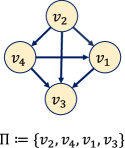
Figure 1: An example of the correspondence between an ordering and a fully-connected DAG.

The problem of finding a directed graph that satisfies the ayclicity constraint can be cast as that of finding a variable ordering Teyssier and Koller (2005); Schmidt et al. (2007). Specifically, let $\Pi$ denote an ordering of the nodes in $V$, where the length of the ordering $|\Pi|=|V|$ and $\Pi$ is indexed from 1. If node $v_{j}\in V$ lies in the $p$-th position, then $\Pi(p)=v_{j}$. Notation $\Pi_{\prec v_{j}}$ denotes the set of nodes that precede node $v_{j}$ in $\Pi$. One can easily establish a canonical correspondence between an ordering $\Pi$ and a fully-connected DAG $\mathcal{G}^{\Pi}$; an example is presented in Figure 1. A DAG $\mathcal{G}$ can be consistent with more than one orderings and the set of these orderings is denoted by

$$\Phi(\Pi)=\{\Pi:~{}\text{fully-connected DAG}~{}\mathcal{G}^{\Pi}~{}\text{is a super-DAG of}\ \mathcal{G}\},$$

where a super-DAG of $\mathcal{G}$ is a DAG whose edge set is a superset of that of $\mathcal{G}$. The the search for the true DAG $\mathcal{G}^{*}$ can be decomposed to two phases: finding the correct ordering and performing variable selection; the latter is to find the optimal DAG that is consistent with the ordering found in the first step.

3.2 Reinforcement Learning

Standard RL is usually formulated as an MDP over the environment state $s\in\mathcal{S}$ and agent action $a\in\mathcal{A}$, under an (unknown) environmental dynamics defined by a transition probability $\mathcal{T}(s^{\prime}|s,a)$. Let $\pi_{\phi}(a|s)$ denote the policy, parameterized by $\phi$, which outputs a distribution used to select an action from action space $\mathcal{A}$ based on state $s$. For episodic tasks, a trajectory $\tau=\{s_{t},a_{t}\}^{T}_{t=0}$, where $T$ is the finite time horizon, can be collected by executing the policy repeatedly. In many cases, an immediate reward $r(s,a)$ can be received when agent executes an action. The objective of RL is to learn a policy which can maximize the expected cumulative reward along a trajectory, i.e., $J(\phi)=\mathbb{E}_{\pi_{\phi}}[R_{0}]$ with $R_{0}=\sum^{T}_{t=0}\gamma^{t}r_{t}(s_{t},a_{t})$ and $\gamma\in(0,1]$ being a discount factor. For some scenarios, the reward is only earned at the terminal time (also called episodic reward), and $J(\phi)=\mathbb{E}_{\pi_{\phi}}[R(\tau)]$ with $R(\tau)=r_{T}(s_{T},a_{T})$.

4 Method

In this section, we first formulate the ordering search problem as an MDP and then describe the proposed approach. We also discuss the variable selection methods to obtain DAGs from variable orderings, as well as the consistency and computational complexity regarding the proposed method.

4.1 Ordering Search as Markov Decision Process

To incorporate RL into the ordering-based paradigm, we formulate the variable ordering search problem as a multi-step decision process with a variable as an action at each decision step, and the order of the selected actions (or variables) is treated as the searched ordering. The decision-making process is Markovian, and its elements are described as follows.

State.

One can directly take the sample data $\mathbf{x}_{j}$ as the state. However, preliminary experiments (see Appendix A.1) show that it is difficult for feed-forward neural network models to capture the underlying causal relationships directly using observed data as states, and that the data pre-processed by an encoder module is helpful to find better orderings. The encoder module embeds each $\mathbf{x}_{j}$ to state $s_{j}$ and all the embedded states constitute the state space $\mathcal{S}:=\{{s}_{1},\cdots,{s}_{d}\}$. In our case, we also need an initial state, denoted by $s_{0}$ (detailed choice is given in Section 4.2), to select the first action. The complete state space would be $\mathcal{\hat{S}}:=\mathcal{S}\cup\{s_{0}\}$. We will use $\hat{s}_{t}$ to denote the actual state encountered at the $t$-th decision step when generating a variable ordering.

Action.

We select an action (variable) from the action space $\mathcal{A}:=\{{v}_{1},\cdots,{v}_{d}\}$ consisting of all the variables at each decision step, and the action space size is equal to the number of variables, i.e., $|\mathcal{A}|=d$. Compared to the previous RL-based method that searches over the graph space with size $\mathcal{O}(2^{d\times d})$ Zhu et al. (2020), the resulting action space becomes much smaller.

State transition.

The state transition is related to the action selected at the current decision step. If the selected variable is $v_{j}$ at the $t$-th decision step, then the state is transferred to the state $s_{j}\in\mathcal{S}$ which corresponds to $\mathbf{x}_{j}$ embedded by the encoder, i.e., $\hat{s}_{t+1}=s_{j}$.

Reward.

In ordering-based methods, only the variables selected in previous decision steps can be the potential parents of the currently selected variable. Hence, we design the rewards in the following cases: episodic reward and dense reward. In the former case, we calculate the score for a variable ordering $\Pi$ with $d$ variables as the episodic reward, i.e.,

$$R(\tau)=r_{T}(\hat{s}_{T},a_{T})=\text{S}_{\text{BIC}}(\mathcal{G}^{\Pi})$$ (2)

where $T=d-1$ and $\text{S}_{\text{BIC}}$ has been defined in Equation (1), with $\text{Pa}(X_{j})$ replaced by the potential parent variable set $U(X_{j})$; here $U(X_{j})$ denotes the variables associated with the nodes in $\Pi_{\prec v_{j}}$. If the score function is decomposable (e.g., the BIC score), we can calculate an immediate reward by exploiting the decomposability for the current decision step. That is, for $v_{j}$ selected at time step $t$, the immediate reward is

$$r_{t}=\sum^{m}_{k=1}\log p(x^{k}_{j}|U(x_{j}^{k});\theta_{j})-\frac{|\theta_{j}|}{2}\log m.$$ (3)

This belongs the second case with dense rewards. Here we keep $-|\theta_{j}|/2\log m$ to make Equation (3) consistent with the form of BIC score.

4.2 Implementation and Optimization with Reinforcement Learning

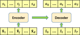
Figure 2: Illustration of the policy model. The encoder embeds the observed data $\mathbf{x}_{j}$ into the state $s_{j}$. An action $a_{t}$ can be selected by the decoder according to the given state $\hat{s}_{t}$ and the pointer mechanism at each time step $t$. Note that $T=d-1$. See Appendix A for details.

We briefly describe the neural network architectures implemented in our method, as shown in Figure 2. More details can be found in Appendix A.

Encoder.

$f_{\phi_{e}}^{\mathrm{enc}}:\tilde{\mathbf{X}}\mapsto\mathcal{S}$ is used to map the observed data to the embedding space $\mathcal{S}=\{s_{1},\cdots,s_{d}\}$. Similar to Zhu et al. (2020), we adopt mini-batch training and randomly draw $n$ samples from $m$ samples of the data set $\mathbf{X}$ to construct $\tilde{\mathbf{X}}\in\mathbb{R}^{n\times d}$ at each episode. We also set the embedding $s_{j}$ to be in the same dimension, i.e., $s_{j}\in\mathbb{R}^{n}$. For encoder choice, we conduct an empirical comparison among several representative structures such as MLP, LSTM and the self-attention based encoder Vaswani et al. (2017). Empirically, we validate that the self-attention based encoder in the Transformer structure performs the best (see Appendix A.1).

Decoder.

$f_{\phi_{d}}^{\text{dec}}:\mathcal{\hat{S}}\mapsto\mathcal{A}$ maps the state space $\mathcal{\hat{S}}$ to the action space $\mathcal{A}$. Among several decoder choices (see also Appendix A.1 for an empirical comparison), we pick an LSTM based structure that proves effective in our experiments. Although the initial state is generated randomly in many applications, we pick it as $s_{0}=\frac{1}{d}\sum_{i=1}^{d}s_{i}$, considering that the source node is fixed in a correct ordering. We restrict each node only be selected once by masking the selected nodes, in order to generate a valid ordering Vinyals et al. (2015).

Optimization.

The optimization objective is to learn a policy maximizing $J(\phi)$, where $\phi=\{\phi_{e},\phi_{d}\}$ with $\phi_{e}$ and $\phi_{d}$ being parameters associated with encoder $f^{\text{enc}}$ and decoder $f^{\text{dec}}$, respectively. Based on the above definition, policy gradient Sutton and Barto (2018) is used to optimize the ordering generation model parameters. For the episodic reward case, we have the following policy gradient $\nabla J(\phi)=\mathbb{E}_{\pi_{\phi}}\left[R(\tau)\sum^{T}_{t=0}\nabla_{\phi}\log\pi_{\phi}\left(a_{t}|\hat{s}_{t}\right)\right]$, and the algorithm in this case is denoted as CORL-1. For the dense reward case, policy gradient can be calculated as $\nabla J(\phi)=\mathbb{E}_{\pi_{\phi}}\left[\sum^{T}_{t=0}R_{t}\nabla_{\phi}\log\pi_{\phi}\left(a_{t}|\hat{s}_{t}\right)\right]$, where $R_{t}=\sum^{T-t}_{l=0}\gamma^{l}r_{t+l}$ denotes the return at time step $t$. We denote the algorithm in this case as CORL-2. Using a parametric baseline to estimate the expected score typically improves learning Sutton and Barto (2018). Therefore, we introduce a critic network $V_{\phi_{v}}(\hat{s}_{t})$ parameterized by $\phi_{v}$, which learns the expected return given state $\hat{s}_{t}$ and is trained with stochastic gradient descent using Adam optimizer on a mean squared error objective between its predicted value and the actual return. More details about the critic network are described in Appendix A.2.

Inspired by the benefits from pretrained models Bello et al. (2016), we also consider to incorporate pretraining to our method to accelerate training. In practice, one can usually obtain some observed data with known causal graphs or correct orderings, e.g., by simulation or real data with labeled graphs. Hence, we can pretrain a policy model with such data in a supervised way and use the pretrained model as initialization for new tasks. Meanwhile, a sufficient generalization ability is desired and we hence include diverse data sets with different numbers of nodes, noise types, causal relationships, etc.

4.3 Variable Selection

			RANDOM	NOTEARS	DAG-GNN	RL-BIC2	L1OBS	A* Lasso	CORL-1	CORL-2
30 nodes	ER2	TPR	0.41 (0.04)	0.95 (0.03)	0.91 (0.05)	0.94 (0.05)	0.78 (0.06)	0.88 (0.04)	0.99 (0.02)	0.99 (0.01)
		SHD	140.4 (36.7)	14.2 (9.4)	26.5 (12.4)	17.8 (22.5)	85.2 (23.8)	35.3 (14.3)	5.2 (7.4)	4.4 (3.5)
	ER5	TPR	0.43 (0.03)	0.93 (0.01)	0.85 (0.11)	0.91 (0.03)	0.74 (0.04)	0.84 (0.05)	0.94 (0.03)	0.95 (0.03)
		SHD	210.2 (43.5)	35.4 (7.3)	68.0 (39.8)	45.6 (13.3)	98.6 (32.7)	71.2 (21.5)	37.4 (16.9)	37.6 (14.5)
	SF2	TPR	0.58 (0.02)	0.98 (0.02)	0.92 (0.09)	0.99 (0.02)	0.83 (0.04)	0.93 (0.02)	1.0 (0.01)	1.0 (0.01)
		SHD	118.4 (12.3)	6.1 (2.3)	36.8 (33.1)	3.2 (1.7)	49.7 (28.1)	27.3 (18.4)	0.0 (0.0)	0.0 (0.0)
	SF5	TPR	0.44 (0.03)	0.94 (0.03)	0.89 (0.09)	0.96 (0.03)	0.79 (0.04)	0.88 (0.03)	1.00 (0.00)	1.00 (0.00)
		SHD	165.4 (10.6)	23.3 (6.9)	47.8 (35.2)	11.3 (5.2)	89.3 (25.7)	40.5 (19,8)	0.0 (0.0)	0.0 (0.0)
100 nodes	ER2	TPR	0.33 (0.05)	0.93 (0.02)	0.93 (0.03)	0.02 (0.01)	0.54 (0.02)	0.86 (0.04)	0.98 (0.02)	0.98 (0.01)
		SHD	491.4 (17.6)	72.6 (23.5)	66.2 (19.2)	270.8 (13.5)	481.2 (49.9)	128.5 (38.4)	24.8 (10.1)	18.6 (5.7)
	ER5	TPR	0.34 (0.04)	0.91 (0.01)	0.86 (0.16)	0.08 (0.03)	0.53 (0.02)	0.82 (0.05)	0.93 (0.02)	0.94 (0.03)
		SHD	984.4 (35.7)	170.3 (34.2)	236.4 (36.8)	421.2 (46.2)	547.9 (63.4)	244.0 (42.3)	175.3 (18.9)	164.8 (17.1)
	SF2	TPR	0.48 (0.03)	0.98 (0.01)	0.89 (0.14)	0.04 (0.02)	0.57 (0.03)	0.92 (0.03)	1.00 (0.00)	1.00 (0.00)
		SHD	503.4 (23.8)	2.3 (1.3)	156.8 (21.2)	281.2 (17.4)	377.3 (53.4)	54.0 (22.3)	0.0 (0.0)	0.0 (0.0)
	SF5	TPR	0.47 (0.04)	0.95 (0.01)	0.87 (0.15)	0.05 (0.03)	0.55 (0.04)	0.89 (0.03)	0.97 (0.02)	0.98 (0.01)
		SHD	891.3 (19.4)	90.2 (34.5)	165.2 (22.0)	405.2 (77.4)	503.7 (56.4)	114.0 (36.4)	19.4 (5.2)	10.8 (6.1)

Table 1: Empirical results for ER and SF graphs of $30$ and $100$ nodes with LG data.

One can obtain the causal graph from an ordering by conducting variable selection methods, such as sparse candidate Teyssier and Koller (2005), significance testing of covariates Bühlmann et al. (2014), and group Lasso Schmidt et al. (2007). In this work, for linear data models, we apply linear regression to the obtained fully-connected DAG and then use thresholding to prune edges with small weights, as similarly used by Zheng et al. (2018). For the non-linear model, we adopt the CAM pruning used by Lachapelle et al. (2020). For each variable $X_{j}$, one can fit a generalized additive model against the current parents of $X_{j}$ and then apply significance testing of covariates, declaring significance if the reported p-values are lower that or equal to $0.001$. The overall method is summarized in Algorithm 1.

Algorithm 1 Causal discovery with Ordering-based RL.

0:  observed data $\mathbf{X}$, initial parameters $\phi_{e},\phi_{d}$ and $\phi_{v}$, two empty buffers $\mathcal{D}$ and $\mathcal{D}_{score}$, initial value (negative infinite) BestScore and a random ordering BestOrdeing.

1:  while not terminated do

2:     draw a batch of samples from $\mathbf{X}$, encode them to $\mathcal{S}$ and calculate the initial state $\hat{s}_{0}$

3:     for $t=0,1,\ldots,T$ do

4:        collect a batch of data $\langle\hat{s}_{t},a_{t},r_{t}\rangle$ with $\pi_{\phi}$: $\mathcal{D}=\mathcal{D}\cup\{\langle\hat{s}_{t},a_{t},r_{t}\rangle\}$

5:        if $\langle v_{t},\Pi_{\prec v_{t}},r_{t}\rangle$ is not in $\mathcal{D}_{score}$ then

6:           store $\langle v_{t},\Pi_{\prec v_{t}},r_{t}\rangle$ in $\mathcal{D}_{score}$

7:        end if

8:     end for

9:     update $\phi_{e},\phi_{d}$, and $\phi_{v}$ as described in Section 4.2

10:     if $\sum^{T}_{t=0}r_{t}>\text{BestScore}$ then

11:        update the BestScore and BestOrdering

12:     end if

13:  end while

14:  get the final DAG by pruning the BestOrdering

4.4 Consistency Analysis

So far we have presented CORL in a general manner without specifying explicitly the distribution family for calculating the scores or rewards. In principle, any distribution family could be employed as long as its log-likelihood can be computed. However, whether the maximization of the accumulated reward recovers the correct ordering, i.e., whether consistency of the score function holds, depends on both the modelling choice of reward and the underlying SEM. If the SEM is identifiable, then the following proposition shows that it is possible to find the correct ordering with high probability in the large sample limit.

Proposition 1.

Suppose that an identifiable SEM with true causal DAG $\mathcal{G}^{*}$ on $X=\{X_{j}\}_{j=1}^{d}$ induces distribution $P(X)$. Let $\mathcal{G}^{\Pi}$ be the fully-connected DAG that corresponds to an ordering $\Pi$. If there is an SEM with $\mathcal{G}^{\Pi}$ inducing the same distribution $P(X)$, then $\mathcal{G}^{\Pi}$ must be a super-graph of $\mathcal{G}^{*}$, i.e., every edge in $\mathcal{G}^{*}$ is covered in $\mathcal{G}^{\Pi}$.

Proof.

The SEM with $\mathcal{G}^{\Pi}$ may not be causally minimal but can be reduced to an SEM satisfying the causal minimality condition Peters et al. (2014). Let $\tilde{\mathcal{G}}^{\Pi}$ denotes the causal graph in the reduced SEM with the same distribution $P(X)$. Since we have assumed that original SEM is identifiable, i.e., the distribution $P(X)$ corresponds to a unique true graph, $\tilde{\mathcal{G}}^{\Pi}$ is then identical to $\mathcal{G}^{*}$. The proof is complete by noticing that $\mathcal{G}^{\Pi}$ is a super-graph of $\tilde{\mathcal{G}}^{\Pi}$. ∎

Thus, if the causal relationships fall into the chosen model functions and a right distribution family is assumed, then given infinite samples the optimal accumulated reward (e.g., the optimal BIC score) must be achieved by a super-DAG of the underlying graph. However, finding the optimal accumulated reward may be hard, because policy gradient methods only guarantee local convergence Sutton and Barto (2018), and we can only apply approximate model functions and also need to assume a certain distribution family for calculating the reward. Nevertheless, the experimental results in Section 5 show that the proposed method can achieve a better performance than those with consistency guarantee in the finite sample regime, thanks to the improved search ability of modern RL methods.

4.5 Computational Complexity

In contrast with typical RL applications, we treat RL here as a search strategy, aiming to find an ordering that achieves the best score. CORL requires the evaluation of the rewards at each episode with $\mathcal{O}(dm^{2}+d^{3})$ computational cost if linear functions are adopted to model the causal relations, which is same to RL-BIC2 Zhu et al. (2020). Fortunately, CORL does not need to compute the matrix exponential term with $\mathcal{O}(d^{3})$ cost due to the use of ordering search. We observe that CORL performs fewer episodes than RL-BIC2 before the episode reward converges (see Appendix C). The evaluation of Transformer encoder and LSTM decoder in CORL take $\mathcal{O}(nd^{2})$ and $\mathcal{O}(dn^{2})$, respectively. However, we find that computing rewards is dominating in the total running time (e.g., around $95\%$ and $87\%$ for $30$- and $100$-node linear data models). Thus, we record the decomposed scores for each variable $v_{j}$ with different parental sets $\Pi_{\prec v_{j}}$ to avoid repeated computations.

5 Experiments

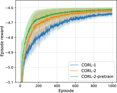
Figure 3: Learning curves of CORL-1, CORL-2 and CORL-2-pretrain on $100$-node LG data sets.

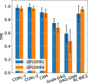
(a) TPR on GP10

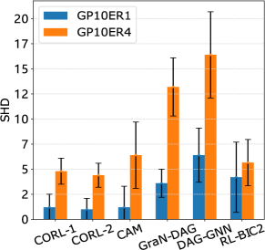
(b) SHD on GP10

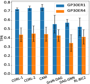
(c) TPR on GP30

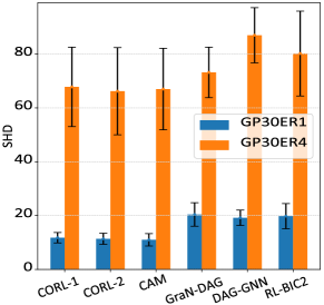
(d) SHD on GP30

Figure 4: The empirical results on GP data models with 10 and 30 nodes.

In this section, we conduct experiments on synthetic data sets with linear and non-linear causal relationships as well as a real data set. The baselines are ICA-LiNGAM Shimizu et al. (2006), three ordering-based approaches L1OBS Schmidt et al. (2007), CAM Bühlmann et al. (2014) and A* Lasso Xiang and Kim (2013), some recent gradient-based approaches NOTEARS Zheng et al. (2018), DAG-GNN Yu et al. (2019) and GraN-DAG Lachapelle et al. (2020), and the RL-based approach RL-BIC2 Zhu et al. (2020). We use the original implementations (see Appendix B.1 for details) and pick the recommended hyper-parameters unless otherwise stated.

We generate different types of synthetic data sets which vary along: level of edge sparsity, graph type, number of nodes, causal functions and sample size. Two types of graph sampling schemes, Erdös–Rényi (ER) and Scale-free (SF), are considered here. We denote $d$-node ER and SF graphs with on average $hd$ edges as ER$h$ and SF$h$, respectively. Two common metrics are considered: True Positive Rate (TPR) and Structural Hamming Distance (SHD). The former indicates the probability of correctly finding the positive edges among the discoveries. Hence, it can be used to measure the quality of an ordering, and the higher the better. The latter counts the total number of missing, falsely detected or reversed edges, and the smaller the better.

5.1 Linear Models with Gaussian and Non-Gaussian Noise

We evaluate the proposed methods on Linear Gaussian (LG) with equal variance Gaussian noise and LiNGAM data models, and the true DAGs in both cases are known to be identifiable Peters and Bühlmann (2014); Shimizu et al. (2006). We set $h\in\{2,5\}$ and $d\in\{30,50,100\}$ to generate observed data (see Appendix B.2 for details). For variable selection, we set the thresholding as $0.3$ and apply it to the estimated coefficients, as similarly used by Zheng et al. (2018); Zhu et al. (2020).

Table 1 presents the results for $30$- and $100$-node LG data models; the conclusions do not change with $50$-node graphs, which are given in Appendix D. The performances of ICA-LiNGAM, GraN-DAG and CAM is also given in Appendix D, and they are almost never on par with the best methods presented in this section. CORL-1 and CORL-2 achieve consistently good results on LiNGAM data sets which are reported in Appendix E due to the space limit.

We now examine Table 1 (the values in parentheses represent the standard deviation across data sets per task). Across all settings, CORL-1 and CORL-2 are the best performing methods in terms of both TPR and SHD, while NOTEARS and DAG-GNN are not too far behind. In Figure 3, we further show the training reward curves of CORL-1 and CORL-2 on $100$-node LG data sets, where CORL-2 converges faster to a better ordering than CORL-1. We conjecture that this is because dense rewards can provide more guidance information for the training process than episodic rewards, which is beneficial to the learning of RL model and improves the training performance. Hence, CORL-2 is preferred in practice if the score function is decomposable for each variable. As discussed previously, RL-BIC2 only achieves satisfactory results on graphs with $30$ nodes. The TPR of L1OBS is lower than that of A* Lasso, which indicates that L1OBS using greedy hill-climbing with tabu lists may not find a good ordering. Note that the SHD of L1OBS and A* Lasso reported here are the results after applying the introduced pruning method. We observe that the SHDs are greatly improved after pruning. For example, the SHDs of L1OBS decrease from $171.6$ $(29.5)$, $588.0$ $(66.2)$ and $1964.5$ $(136.6)$ to $85.2$ $(23.8)$, $215.4$ $(26.3)$ and $481.2$ $(49.9)$ for ER2 graphs with $30$, $50$ and $100$ nodes, respectively, while the TPRs almost keep the same.

We have also evaluated our method on $150$-node LG data models on ER2 graphs. CORL-1 has TPR and SHD being $0.95$ $(0.01)$ and $63.7$ $(9.1)$, while CORL-2 has $0.97$ $(0.01)$ and $38.3$ $(14.3)$, respectively. CORL-2 outperforms NOTEARS that achieves $0.94$ $(0.02)$ and $50.8$ $(21.8)$.

Pretraining.

We show the training reward curve of CORL-2-pretrain in Figure 3, where the model parameters are pretrained in a supervised manner. The data sets used for pretraining contain $30$-node ER2 and SF2 graphs with different causal relationships. Note that the data sets used for evaluation are different from those used for pretraining. Compared to that of CORL-2 using random initialization, a pretrained model can accelerate the model learning process. Although pretraining requires additional time, it is only carried out once and when finished, the pretrained model can be used for multiple causal discovery tasks. Similar conclusion can be drawn in terms of CORL-1, which is shown in Appendix G.

Running time.

We also report the running time of all the methods on $30$- and $100$-node linear data models: CORL-1, CORL-2, GraN-DAG and DAG-GNN $\approx$ $15$ minutes for $30$-node graphs; CORL-1 and CORL-2 $\approx$ $7$ hours against GraN-DAG and DAG-GNN $\approx$ $4$ hours for $100$-node graphs; CAM $\approx$ $15$ minutes for both $30$- and $100$-node graphs, while L1OBS and A* Lasso $\approx$ $2$ minutes for that tasks; NOTEARS $\approx$ $5$ minutes and $\approx$ $1$ hour for the two tasks respectively; RL-BIC2 $\approx$ $3$ hours for $30$-node graphs. We set the maximal running time up to $15$ hours, but RL-BIC2 did not converge on $100$-node graphs, hence we did not report its results. Note that the running time can be significantly reduced by paralleling the evaluation of reward. The neural network based learning methods generally take longer time, and the proposed method achieves the best performance among these methods.

5.2 Non-Linear Model with Gaussian Process

In this experiment, we consider causal relationships with $f_{j}$ being a function sampled from a Gaussian Process (GP) with radial basis function kernel of bandwidth one. The additive noise follows standard Gaussian distribution, which is known to be identifiable Peters et al. (2014). We consider ER1 and ER4 graphs with different sample numbers (see Appendix B.2 for the generation of data sets), and we only report the results with $m=500$ samples due to the space limit (the remaining results are given in Appendix F). For comparison, only the methods that have been shown competitive for this non-linear data model in existing works Zhu et al. (2020); Lachapelle et al. (2020) are included. For a given ordering, we follow Zhu et al. (2020) to use GP regression to fit the causal relationships. We also set a maximum time limit of $15$ hours for all the methods for fair comparison and only graphs with up to $30$ nodes are considered here, as using GP regression to calculate the scores is time-consuming. The variable selection method used here is the CAM pruning from Bühlmann et al. (2014).

The results on $10$- and $30$-node data sets with ER1 and ER4 graphs are shown in Figure 4. Overall, both GraN-DAG and DAG-GNN perform worse than CAM. We conjecture that this is because the number of samples are not sufficient for GraN-DAG and DAG-GNN to fit neural networks well, as also shown by Lachapelle et al. (2020). CAM, CORL-1, and CORL-2 have similar results, with CORL-2 performing the best on $10$-node graphs and being slightly worse than CAM on $30$-node graphs. All of these methods have better results on ER1 graphs than on ER4 graphs, especially with $30$ nodes. We also notice that CORL-2 only runs about $700$ iterations on $30$-node graphs and about $5000$ iterations on $10$-node graphs within the time limit, due to the increased time from GP regression. Nonetheless, the proposed method achieves a much improved performance compared with the existing RL-based method.

5.3 Real Data

The Sachs data set Sachs et al. (2005), with $11$-node and $17$-edge true graph, is widely used for research on graphical models. The expression levels of protein and phospholipid in the data set can be used to discover the implicit protein signal network. The observational data set has $m=853$ samples and is used to discover the causal structure. We similary use Gaussian Process regression to model the causal relationships in calculating the score. In this experiment, CORL-1, CORL-2 and RL-BIC2 achieve the best SHD $11$. CAM, GraN-DAG, and ICA-LiNGAM achieve SHDs $12$, $13$ and $14$, respectively. Particularly, DAG-GNN and NOTEARS result in SHDs $16$ and $19$, respectively, whereas an empty graph has SHD $17$.

6 Conclusion

In this work, we have incorporated RL into the ordering-based paradigm for causal discovery, where a generated ordering can be pruned by variable selection to obtain the causal DAG. Two methods are developed based on the MDP formulation and an encoder-decoder framework. We further analyze the consistency and computational complexity for the proposed approach. Empirical results validate the improved performance over existing RL-based causal discovery approach.

References

- Bartlett and Cussens [2017] Mark Bartlett and James Cussens. Integer linear programming for the bayesian network structure learning problem. Artificial Intelligence, 244:258–271, 2017.
- Bello et al. [2016] Irwan Bello, Hieu Pham, Quoc V Le, Mohammad Norouzi, and Samy Bengio. Neural combinatorial optimization with reinforcement learning. arXiv preprint arXiv:1611.09940, 2016.
- Bernstein et al. [2020] Daniel Bernstein, Basil Saeed, Chandler Squires, and Caroline Uhler. Ordering-based causal structure learning in the presence of latent variables. In International Conference on Artificial Intelligence and Statistics (AISTATS), pages 4098–4108. PMLR, 2020.
- Bühlmann et al. [2014] Peter Bühlmann, Jonas Peters, Jan Ernest, et al. CAM: Causal additive models, high-dimensional order search and penalized regression. The Annals of Statistics, 42(6):2526–2556, 2014.
- Chickering [1996] David Maxwell Chickering. Learning Bayesian networks is NP-complete. In Learning from Data: Artificial Intelligence and Statistics V. Springer, 1996.
- Chickering [2002] David Maxwell Chickering. Optimal structure identification with greedy search. Journal of Machine Learning Research, 3(Nov):507–554, 2002.
- De Campos and Ji [2011] Cassio P De Campos and Qiang Ji. Efficient structure learning of bayesian networks using constraints. The Journal of Machine Learning Research, 12:663–689, 2011.
- Friedman and Koller [2003] Nir Friedman and Daphne Koller. Being Bayesian about network structure. A Bayesian approach to structure discovery in Bayesian networks. Machine learning, 50(1-2):95–125, 2003.
- Khalil et al. [2017] Elias Khalil, Hanjun Dai, Yuyu Zhang, Bistra Dilkina, and Le Song. Learning combinatorial optimization algorithms over graphs. In Advances in Neural Information Processing Systems (NeurIPS), 2017.
- Kool et al. [2019] Wouter Kool, Herke Van Hoof, and Max Welling. Attention, learn to solve routing problems! In International Conference on Learning Representations (ICLR), 2019.
- Lachapelle et al. [2020] Sébastien Lachapelle, Philippe Brouillard, Tristan Deleu, and Simon Lacoste-Julien. Gradient-based neural DAG learning. In International Conference on Learning Representations (ICLR), 2020.
- Larranaga et al. [1996] Pedro Larranaga, Cindy MH Kuijpers, Roberto H Murga, and Yosu Yurramendi. Learning bayesian network structures by searching for the best ordering with genetic algorithms. IEEE Transactions on Systems, Man, and Cybernetics-Part A: Systems and Humans, 26(4):487–493, 1996.
- Ng et al. [2019a] Ignavier Ng, Zhuangyan Fang, Shengyu Zhu, Zhitang Chen, and Jun Wang. Masked gradient-based causal structure learning. arXiv preprint arXiv:1910.08527, 2019.
- Ng et al. [2019b] Ignavier Ng, Shengyu Zhu, Zhitang Chen, and Zhuangyan Fang. A graph autoencoder approach to causal structure learning. arXiv preprint arXiv:1911.07420, 2019.
- Peters and Bühlmann [2014] Jonas Peters and Peter Bühlmann. Identifiability of gaussian structural equation models with equal error variances. Biometrika, 101(1):219–228, 2014.
- Peters et al. [2014] Jonas Peters, Joris M. Mooij, Dominik Janzing, and Bernhard Schölkopf. Causal discovery with continuous additive noise models. Journal of Machine Learning Research, 15(1):2009–2053, January 2014.
- Raskutti and Uhler [2018] Garvesh Raskutti and Caroline Uhler. Learning directed acyclic graph models based on sparsest permutations. Stat, 7(1):e183, 2018.
- Sachs et al. [2005] Karen Sachs, Omar Perez, Dana Pe’er, Douglas A Lauffenburger, and Garry P Nolan. Causal protein-signaling networks derived from multiparameter single-cell data. Science, 308(5721):523–529, 2005.
- Scanagatta et al. [2015] Mauro Scanagatta, Cassio P de Campos, Giorgio Corani, and Marco Zaffalon. Learning bayesian networks with thousands of variables. In NeurIPS, 2015.
- Schmidt et al. [2007] Mark Schmidt, Alexandru Niculescu-Mizil, Kevin Murphy, et al. Learning graphical model structure using L1-regularization paths. In Proceedings of the AAAI Conference on Artificial Intelligence (AAAI), 2007.
- Shimizu et al. [2006] Shohei Shimizu, Patrik O Hoyer, Aapo Hyvärinen, and Antti Kerminen. A linear non-Gaussian acyclic model for causal discovery. Journal of Machine Learning Research, 7(Oct):2003–2030, 2006.
- Solus et al. [2017] Liam Solus, Yuhao Wang, and Caroline Uhler. Consistency guarantees for greedy permutation-based causal inference algorithms. arXiv preprint arXiv:1702.03530, 2017.
- Sutton and Barto [2018] Richard S Sutton and Andrew G Barto. Reinforcement Learning: An Introduction. MIT press, 2018.
- Teyssier and Koller [2005] Marc Teyssier and Daphne Koller. Ordering-based search: A simple and effective algorithm for learning bayesian networks. In Conference on Uncertainty in Artificial Intelligence (UAI), 2005.
- Vaswani et al. [2017] Ashish Vaswani, Noam Shazeer, Niki Parmar, Jakob Uszkoreit, Llion Jones, Aidan N Gomez, Łukasz Kaiser, and Illia Polosukhin. Attention is all you need. In Advances in Neural Information Processing Systems (NeurIPS), 2017.
- Vinyals et al. [2015] Oriol Vinyals, Meire Fortunato, and Navdeep Jaitly. Pointer networks. In Advances in Neural Information Processing Systems (NeurIPS), 2015.
- Xiang and Kim [2013] Jing Xiang and Seyoung Kim. A* lasso for learning a sparse bayesian network structure for continuous variables. In Advances in Neural Information Processing Systems (NeurIPS), 2013.
- Yu et al. [2019] Yue Yu, Jie Chen, Tian Gao, and Mo Yu. DAG-GNN: DAG structure learning with graph neural networks. In International Conference on Machine Learning (ICML), 2019.
- Zheng et al. [2018] Xun Zheng, Bryon Aragam, Pradeep K Ravikumar, and Eric P Xing. DAGs with NO TEARS: Continuous optimization for structure learning. In Advances in Neural Information Processing Systems (NeurIPS), 2018.
- Zheng et al. [2020] Xun Zheng, Chen Dan, Bryon Aragam, Pradeep Ravikumar, and Eric P Xing. Learning sparse nonparametric DAGs. In International Conference on Artificial Intelligence and Statistics (AISTATS), 2020.
- Zhu et al. [2020] Shengyu Zhu, Ignavier Ng, and Zhitang Chen. Causal discovery with reinforcement learning. In International Conference on Learning Representations (ICLR), 2020.
- Zoph and Le [2017] Barret Zoph and Quoc V Le. Neural architecture search with reinforcement learning. In International Conference on Learning Representations (ICLR), 2017.