Near- and far-field expansions for stationary solutions of Poisson–Nernst–Planck equations

Abstract

This work is concerned with the stationary Poisson–Nernst–Planck equation with a large parameter which describes a huge number of ions occupying an electrolytic region. Firstly, we focus on the model with a single specie of positive charges in one-dimensional bounded domains due to the assumption that these ions are transported in the same direction along a tubular-like mircodomain, as was introduced in [2]. We show that the solution asymptotically blows up in a thin region attached to the boundary, and establish the refined “near-field” and “far-field” expansions for the solutions with respect to the parameter. Moreover, we obtain the boundary concentration phenomenon of the net charge density, which mathematically confirms the physical description that the non-neutral phenomenon occurs near the charged surface. In addition, we revisit a nonlocal Poisson–Boltzmann model for monovalent binary ions (cf. [26, 28]) and establish a novel comparison for these two models.
Key words. Stationary PNP equation, Large parameter, Near-field asymptotics, Far-field asymptotics, Non-neutral phenomenon
AMS subject classifications. 35M33, 35B25, 35Q92, 35R09, 78A25

1 Introduction

With the development of current nanotechnology in electrochemistry [11, 38], analysis of solutions to mathematical models with regulated parameters plays a more and more important role in investigating the distribution of electrostatic potential in electrolyte-like solutions (cf. [7, 13, 16, 18, 22, 35, 41, 43, 45]). In the past few decades, a key ingredient for understanding of such microscopic phenomena is the Poisson–Boltzmann equation [4, 44, 46], but which suffered from deficiencies that are well known. Different types of nonlinear electrochemistry systems (see, e.g., [5, 9, 14, 15, 17, 19, 20, 27, 32, 33, 36, 39, 40, 42]) have already been modeled and the corresponding computational confirmation is expected to reach theoretical prediction.

Among such phenomena in electrochemistry, an unstable one relates to the non-electroneutrality characterized by the localization of excess charge distributions. For instance, a faradaic current drives ions from one electrode surface to another and results in an ionic distribution which is non-uniform near the electrode surface. We refer the reader to [8, 31]. Other instabilities including the electroconvective instability in channels have been investigated; see, e.g., [34] and references therein. Despite the intensive investigation yielding detailed information and the reasonable success, little is known about the non-electroneutral phenomenon near the charged surface. In [2, 3], employing the one dimensional Poisson–Nernst–Planck (PNP) system provides an underlying framework for such phenomena, where it is reasonably assumed that all ions transport in the same direction along a tubular-like mircodomain with finite-length so that the physical domain can be set as a one-dimensional interval $\Omega=(0,1)$. At the beginning of this work we consider the model for single-ion species which is represented as

$$\left\{\begin{aligned} &\quad\,\,\,\,\frac{\partial{p}}{\partial{t}}(t,r)=D_{p}\frac{\partial}{\partial{r}}\left(\frac{\partial{p}}{\partial{r}}(t,r)+\frac{z_{p}\mathrm{e}_{0}}{k_{B}T}p(t,r)\frac{\partial{u}}{\partial{r}}(t,r)\right),\\ &-\frac{\partial^{2}{u}}{\partial{r}^{2}}(t,r)=\boldsymbol{\lambda}(\rho_{\text{f}}(r)+z_{p}\mathrm{e}_{0}p(t,r)),\quad\quad\quad(t,r)\in(0,\infty)\times(0,1),\end{aligned}\right.$$ (1.1)

with the no-flux boundary conditions

$$\left(\frac{\partial{p}}{\partial{r}}+\frac{z_{p}\mathrm{e}_{0}}{k_{B}T}p\frac{\partial{u}}{\partial{r}}\right)(t,0)=\left(\frac{\partial{p}}{\partial{r}}+\frac{z_{p}\mathrm{e}_{0}}{k_{B}T}p\frac{\partial{u}}{\partial{r}}\right)(t,1)=0,\,\,t>0,$$ (1.2)

and initial conditions $p(0,r)=p_{0}(r)>0$ and $u(0,r)=u_{0}(r)$, for $r\in[0,1]$, which are compatible with the boundary conditions (1.2). Notice that (1.1)–(1.2) satisfies shift in variance in $u$ and so we will set the boundary condition for $u$ later.

Physically, $u$ is the electrostatic potential, $p$ is the density of cations, $D_{p}$ is the diffusion coefficient, $z_{p}$ is the valency of cations, $\mathrm{e}_{0}$ is the elementary charge, $k_{B}$ is the Boltzmann constant, $T$ is the absolute temperature, and $\rho_{\text{f}}$ is the fixed permanent charge density in the physical domain. Besides, $\boldsymbol{\lambda}=d^{2}\mathrm{e}_{0}S/(\varepsilon_{0}U_{T})$ where $\varepsilon_{0}$ is the dielectric constant of the electrolyte, $U_{T}$ is the thermal voltage, $d$ is the diameter of the domain $\Omega=\left(0,1\right)$, and $S$ is the appropriate concentration scale [37]. Note that the no-flux boundary conditions (1.2) ensure the conservation of ions, i.e.,

$$\int_{0}^{1}p(t,r)\mathrm{d}r=\int_{0}^{1}p_{0}(r)\mathrm{d}r,\,\,\forall\,t>0.$$ (1.3)

To see the non-electroneutral phenomenon near the charged surface, $\boldsymbol{\lambda}$ is assumed a large positive parameter corresponding to the number of ions occupying an electrolytic region, as was studied in [2]. To basically understand the non-electroneutral phenomenon of $u$ and $p$ as $\boldsymbol{\lambda}\gg 1$, we neglect the effect of fixed permanent charges by setting $\rho_{\text{f}}=0$ and focus mainly on their steady-state solutions. Under the standard dimensionless formulation, we may set

$$z_{p}=1,\,\,\mathrm{e}_{0}/k_{B}T=1,\,\,D_{p}=1,$$ (1.4)

and regard $\boldsymbol{\lambda}$ as a positive parameter. Without loss of generality, we may assume $\int_{0}^{1}p_{0}(r)\mathrm{d}r=1$. Then by (1.3) and (1.4), the steady-states of (1.1)–(1.2) verify $u(t,r)=u_{\boldsymbol{\lambda}}(r)$ and the nonlocal relation $p(t,r)=\frac{e^{-u_{\boldsymbol{\lambda}}(r)}}{\int_{0}^{1}e^{-u_{\boldsymbol{\lambda}}(s)}\text{d}s}$ (see also, [1, equation (1.1) with $p=1$], [2, Section 2.1] and [28] and references therein). As a consequence, $u_{\boldsymbol{\lambda}}$ satisfies

$$-u_{\boldsymbol{\lambda}}^{\prime\prime}(r)=\rho_{\boldsymbol{\lambda}}(r):=\frac{\boldsymbol{\lambda}e^{-u_{\boldsymbol{\lambda}}(r)}}{\int_{0}^{1}e^{-u_{\boldsymbol{\lambda}}(s)}\mbox{d}s},~{}r\in(0,1).$$ (1.5)

Physically, $\rho_{\boldsymbol{\lambda}}$ represents the net charge density of the ion species and the parameter $\int_{0}^{1}\rho_{\boldsymbol{\lambda}}(r)\mbox{d}r$ denotes the total charges of ions. It should be mentioned that in [12, Chapter 10.6.1], (1.5) is named the reverse Liouville–Bratú–Gelfand (LBG) equation which can be regarded as the nonlocal LBG equation (see, e.g., [21] and references therein).

For (1.5), we consider the following condition at $r=0$:

$$u_{\boldsymbol{\lambda}}\left(0\right)=u_{\boldsymbol{\lambda}}^{\prime}\left(0\right)=0,$$ (1.6)

as was presented in [2], where assumption $u_{\boldsymbol{\lambda}}(0)=0$ is actually due to a fact that equation (1.5) satisfies the shift invariance; that is, for any $c\in\mathbb{R}$, $u_{\boldsymbol{\lambda}}+c$ also satisfies (1.5). We emphasize that such a setting immediately implies

$$u_{\boldsymbol{\lambda}}^{\prime}(1)=-\boldsymbol{\lambda}.$$ (1.7)

This along with (1.6) asserts that there exists an interior point $r^{\boldsymbol{\lambda}}_{\mathrm{int}}\in(0,1)$ depending on $\boldsymbol{\lambda}$ such that when $\boldsymbol{\lambda}\to\infty$, the net charge density $\rho_{\boldsymbol{\lambda}}(r^{\boldsymbol{\lambda}}_{\mathrm{int}})=-u_{\boldsymbol{\lambda}}^{\prime\prime}(r^{\boldsymbol{\lambda}}_{\mathrm{int}})=u_{\boldsymbol{\lambda}}^{\prime}(0)-u_{\boldsymbol{\lambda}}^{\prime}(1)=\boldsymbol{\lambda}$ asymptotically blows up. As will be clarified later, such a phenomenon occurs only when $r^{\boldsymbol{\lambda}}_{\mathrm{int}}$ is sufficiently close to the boundary point $r=1$ as $\boldsymbol{\lambda}$ tends to infinity. The boundary blow-up behavior theoretically represents the non-neutral phenomenon near the charged surface. We further refer the reader to [26, 28, 30] for the different boundary blow-up phenomena related models with multiple species under various boundary conditions.

It should be stress that equation (1.5)–(1.6) has recently been studied by J. Cartailler et al [2], who used the phase-plane analysis to obtain the uniqueness of equation (1.5)–(1.6). A more general argument for the uniqueness can also be found in [23]. Moreover, the authors in [2] showed that as $\boldsymbol{\lambda}\to\infty$, the numerical solution to (1.5)–(1.7) develops boundary layers near $r=1$. They further studied the leading order term of the asymptotic expansions of $u_{\boldsymbol{\lambda}}(1)$ with respect to $\boldsymbol{\lambda}\gg 1$, and compared the result with their numerical simulation. However, the more refined pointwise asymptotics for solutions, which is crucial for describing the sharp change of $u_{\boldsymbol{\lambda}}$ near the boundary, remains unclear. The issue will be addressed in detail in this work.

1.1 Near-field and far-field expansions

The main difficulty lies in the lack of available asymptotic analysis for such singularly perturbed nonlocal models, which we shall explain as follows. Firstly, one observes from (1.5) and (1.6) that

$$u_{\boldsymbol{\lambda}}(r),\,\,u_{\boldsymbol{\lambda}}^{\prime}(r),\,\,u_{\boldsymbol{\lambda}}^{\prime\prime}(r)<0,~{}~{}r\in(0,1).$$ (1.8)

In particular, (1.5)–(1.7) and (1.8) imply that $\int_{0}^{1}e^{-u_{\boldsymbol{\lambda}}(s)}\mbox{d}s\geq 1$ and

$$u_{\boldsymbol{\lambda}}(1)=-\log\left(1+\frac{\boldsymbol{\lambda}}{2}\int_{0}^{1}e^{-u_{\boldsymbol{\lambda}}(s)}\mbox{d}s\right)\to-\infty\,\,\mbox{as}\,\,\boldsymbol{\lambda}\to\infty.$$ (1.9)

This illustrates the importance of the refined asymptotic expansions of $\int_{0}^{1}e^{-u_{\boldsymbol{\lambda}}(s)}\mbox{d}s$ with respect to $\boldsymbol{\lambda}\gg 1$. A perspective on obtaining such asymptotics is to consider the following nonlinear eigenvalue problem with $\kappa>0$ (see also, [2, Appendix]):

$$\left\{\begin{aligned} &-U_{\kappa}^{\prime\prime}(r)=\kappa e^{-U_{\kappa}(r)},\quad r\in(0,1),\\ &U_{\kappa}(0)=U_{\kappa}^{\prime}(0)=0.\end{aligned}\right.$$ (1.10)

When $\kappa\in(0,\pi^{2}/2)$, (1.10) has a unique solution $U_{\kappa}(r)=2\log\cos(r\sqrt{\kappa/2})$ which is uniformly bounded on $[0,1]$, and $U_{\kappa}(1)\to-\infty$ as $\kappa$ approaches $\pi^{2}/2$ from the left. However, when $\kappa>\pi^{2}/2$, (1.10) does not have solutions defined in the whole domain $(0,1)$. As a consequence, by (1.9) it is expected that a solution $u_{\boldsymbol{\lambda}}$ of (1.5)–(1.6) satisfies

$$\frac{\boldsymbol{\lambda}}{\int_{0}^{1}e^{-u_{\boldsymbol{\lambda}}(s)}\mathrm{d}s}<\frac{\pi^{2}}{2}\,\,\mathrm{for}\,\,\boldsymbol{\lambda}>0,\,\,\mathrm{and}\,\,\frac{\boldsymbol{\lambda}}{\int_{0}^{1}e^{-u_{\boldsymbol{\lambda}}(s)}\mathrm{d}s}\stackrel{{\scriptstyle\boldsymbol{\lambda}\to\infty}}{{-\!\!\!-\!\!\!-\!\!\!-\!\!\!\rightarrow}}\frac{\pi^{2}}{2}.$$ (1.11)

We will prove (1.11) rigorously and establish a more refined asymptotic expansion of $\int_{0}^{1}e^{-u_{\boldsymbol{\lambda}}(s)}\mathrm{d}s$ with respect to $\boldsymbol{\lambda}\gg 1$; see the detail in (2.1) and Remark 2. Moreover, it yields the limiting equation for (1.5)–(1.6) formally as follows:

$$\begin{cases}-U^{\prime\prime}(r)=\displaystyle\frac{\pi^{2}}{2}e^{-U(r)},~{}~{}r\in(0,1),\\ U(0)=U^{\prime}(0)=0,\end{cases}$$ (1.12)

and the unique solution

$$U(r):=U_{\frac{\pi^{2}}{2}}(r)=2\log\cos\left(\frac{\pi}{2}r\right),\,\,r\in[0,1),$$ (1.13)

represents the zeroth-order outer-solution to (1.5)–(1.6) with respect to $\boldsymbol{\lambda}\gg 1$; see also, Remark 1. In passing we note that $U(r)\to-\infty$ and $U^{\prime}(r)=-\pi\tan(\frac{\pi}{2}r)\to-\infty$ as $r\uparrow 1$, which formally coincide with the boundary asymptotic blow-up behavior of $u_{\boldsymbol{\lambda}}$ and $u_{\boldsymbol{\lambda}}^{\prime}$ obtained respectively in (1.9) and (1.7). In summary, equation (1.5)–(1.6) is a nonlocal singularly perturbed model with small parameter $\frac{1}{\boldsymbol{\lambda}}$ in front of its Laplace operator, and its limiting equation connects to a boundary blow-up problem (1.12).

What we want to point out is that the limiting model (1.12) of (1.5)–(1.6) cannot be directly obtained from applying the standard method of matched asymptotic expansions since the nonlocal coefficient $\frac{\boldsymbol{\lambda}}{\int_{0}^{1}e^{-u_{\boldsymbol{\lambda}}(s)}\text{d}s}$ is involved with the parameter $\boldsymbol{\lambda}$ and its corresponding zeroth order outer solution $U(r)$ diverges near $r=1$. To achieve the pointwise description of $u_{\boldsymbol{\lambda}}$ with respect to $\boldsymbol{\lambda}\gg 1$, our first task is concerned with the asymptotic expansions for the solution $u_{\boldsymbol{\lambda}}$, consisting of the near-field expansion and the far-field expansion. In order for the reader to realize the difference from the method of matched asymptotic expansions, we present the argument as follows:

• The near-field expansion focuses mainly on the refined asymptotics of $u_{\boldsymbol{\lambda}}(r_{p,\alpha}^{\boldsymbol{\lambda}})$ and $u^{\prime}_{\boldsymbol{\lambda}}(r_{p,\alpha}^{\boldsymbol{\lambda}})$, where $\alpha$ and $p$ are positive constants independent of $\boldsymbol{\lambda}$, and

  $$r_{p,\alpha}^{\boldsymbol{\lambda}}=1-\frac{p}{\boldsymbol{\lambda}^{\alpha}}\in(0,1),\,\,\boldsymbol{\lambda}\gg 1,$$ (1.14)

  is sufficiently close to the boundary point $r=1$. Let us emphasize again that as $\boldsymbol{\lambda}\gg 1$, $u_{\boldsymbol{\lambda}}$ develops boundary layers and asymptotically blows up near the boundary $r=1$ so that the asymptotic behavior of $u_{\boldsymbol{\lambda}}$ has dramatic changes in a thin neighborhood of $r=1$. To better understand the structure of boundary layers, we are devoted to the pointwise asymptotics of $u_{\boldsymbol{\lambda}}(r_{p,\alpha}^{\boldsymbol{\lambda}})$ and $u_{\boldsymbol{\lambda}}^{\prime}(r_{p,\alpha}^{\boldsymbol{\lambda}})$ with various $\alpha$ and $p$; see, for example, (1.18) and (1.19). Such a consideration essentially points out the difference between the analysis of (1.5)–(1.6) and the standard singularly perturbed equations.

• the far-field expansion focuses on the refined asymptotics for $u_{\boldsymbol{\lambda}}$ in $\mathcal{C}^{1}(K)$ as $\boldsymbol{\lambda}\to\infty$, where $K$ independent of $\boldsymbol{\lambda}$ is a compact subset of $[0,1)$. We will frequently use the norm $\|\cdot\|_{\mathcal{C}^{1}(D)}$ defined by

  $$\|f\|_{\mathcal{C}^{1}(D)}:=\sup_{D}\left(|f|+|f^{\prime}|\right)$$ (1.15)

  where $D$ is a bounded set of $\mathbb{R}$ and $f\in\mathcal{C}^{1}(D)$. When $D=K$ is a compact subset of $[0,1)$, (1.15) is used for convenience to describe the asymptotic expansions of $u$ in $K$.

We refer the reader to [10, 47] for the more detailed physical background of these two terminologies.

We are now in a position to draw the asymptotic behavior of $u_{\boldsymbol{\lambda}}$. As will be presented in detail in Theorem 2.1, for any compact subset $K$ (independent of $\boldsymbol{\lambda}$) of $[0,1)$, we establish the far-field expansion of $u_{\boldsymbol{\lambda}}$ with the precise asymptotic expansions up to the order of $\frac{1}{\boldsymbol{\lambda}^{2}}$:

$$u_{\boldsymbol{\lambda}}(r)=\,U(r)+\pi{r}\left(\frac{\sin(\pi r)}{\boldsymbol{\lambda}}-\frac{\pi{r}+2\sin(\pi r)}{\boldsymbol{\lambda}^{2}}\right)\sec^{2}\left(\frac{\pi}{2}r\right)+\frac{\widetilde{u}_{\boldsymbol{\lambda}}(r)}{\boldsymbol{\lambda}^{2}}\,\,\,\,\,\mbox{and}\,\,\,\sup_{K}|\widetilde{u}_{\boldsymbol{\lambda}}|\stackrel{{\scriptstyle\boldsymbol{\lambda}\to\infty}}{{-\!\!\!-\!\!\!\longrightarrow}}0,$$ (1.16)

where $U$ defined in (1.13) is the unique solution to (1.12). In contrast to the asymptotics of $u_{\boldsymbol{\lambda}}$ in any compact subset of $[0,1)$, our near-field analysis reveals a totally different asymptotic behaviour of $u_{\boldsymbol{\lambda}}$ near the boundary $r=1$. In Theorem 2.2, we show that $u_{\boldsymbol{\lambda}}$ asymptotically blows up near the boundary $r=1$ and obtain a novel asymptotics

$$u_{\boldsymbol{\lambda}}\left(r_{p,\alpha}^{\boldsymbol{\lambda}}\right)={\min\{2,2\alpha\}}\log\frac{1}{\boldsymbol{\lambda}}+\mathcal{O}_{p,\alpha},$$ (1.17)

where $\mathcal{O}_{p,\alpha}$ depends mainly on $p$ and $\alpha$ and satisfies

$$\limsup_{\boldsymbol{\lambda}\to\infty}|\mathcal{O}_{p,\alpha}|<\infty$$

(see Theorem 2.2 for the detailed expression of $\mathcal{O}_{p,\alpha}$). As it was mentioned previously, we shall stress that the concept of the near-field expansions focus on the pointwise asymptotic behavior of solutions sufficiently near the boundary, which is different from the standard matched inner solution. As a consequence, by (1.16) and (1.17) we know that a strong change of $u_{\boldsymbol{\lambda}}$ with $\boldsymbol{\lambda}\to\infty$ merely occurs near the boundary $r=1$, and there hold: (i) as $0<\alpha<1$, $\displaystyle\lim_{\boldsymbol{\lambda}\to\infty}\textstyle\frac{u_{\boldsymbol{\lambda}}(r_{p,\alpha}^{\boldsymbol{\lambda}})}{\log\boldsymbol{\lambda}^{-1}}=2\alpha$ shows that the blow-up asymptotics of $u_{\boldsymbol{\lambda}}(r_{p,\alpha}^{\boldsymbol{\lambda}})$ varies with $\alpha$; (ii) for $0<\alpha_{1}<\alpha_{2}<1$, interior points $1-{\boldsymbol{\lambda}^{-\alpha_{i}}}$, $i=1,2$, are sufficiently close to the boundary, but the corresponding potential difference $|u_{\boldsymbol{\lambda}}(1-{\boldsymbol{\lambda}^{-\alpha_{1}}})-u_{\boldsymbol{\lambda}}(1-{\boldsymbol{\lambda}^{-\alpha_{2}}})|$ tends to infinity as $\boldsymbol{\lambda}\gg 1$. Furthermore, we show the following properties that emphasize the significant change of $u_{\boldsymbol{\lambda}}$ near the boundary $r=1$ as $\boldsymbol{\lambda}\gg 1$ (which can be obtained from (2.6), (2.8) and (2.10)):

• For $r_{p,\alpha}^{\boldsymbol{\lambda}}$ satisfying (1.14) with $0<\alpha\leq 1$, the second order term of $u_{\boldsymbol{\lambda}}(r_{p,\alpha}^{\boldsymbol{\lambda}})$ (i.e., the leading order term of $\mathcal{O}_{p,\alpha}$ as $\boldsymbol{\lambda}\gg 1$) relies exactly on $p$; however, when $\alpha>1$, the second order term of $u_{\boldsymbol{\lambda}}(r_{p,\alpha}^{\boldsymbol{\lambda}})$ is independent of $p$.

• Various potential differences $|u_{\boldsymbol{\lambda}}(r_{p,\alpha}^{\boldsymbol{\lambda}})-u_{\boldsymbol{\lambda}}(1)|$ and $|u_{\boldsymbol{\lambda}}\left(r_{p_{1};\alpha}^{\boldsymbol{\lambda}}\right)-u_{\boldsymbol{\lambda}}\left(r_{p_{2};\alpha}^{\boldsymbol{\lambda}}\right)|$ with $p_{1}\neq{p}_{2}$ can be presented as follows:

  $$\lim_{\boldsymbol{\lambda}\to\infty}\left|u_{\boldsymbol{\lambda}}(r_{p,\alpha}^{\boldsymbol{\lambda}})-u_{\boldsymbol{\lambda}}\left(1\right)\right|=\begin{cases}\infty,&\mbox{if}\,\,0<\alpha<1,\\ \displaystyle 2\log\frac{p+2}{2},&\mbox{if}\,\,\alpha=1,\\ 0,&\mbox{if}\,\,\alpha>1,\end{cases}$$ (1.18)

  and

  $$\lim_{\boldsymbol{\lambda}\to\infty}\left|u_{\boldsymbol{\lambda}}\left(r_{p_{1};\alpha}^{\boldsymbol{\lambda}}\right)-u_{\boldsymbol{\lambda}}\left(r_{p_{2};\alpha}^{\boldsymbol{\lambda}}\right)\right|=\begin{cases}\displaystyle 2\left|\log\frac{p_{1}}{p_{2}}\right|,&\mbox{if}\,\,0<\alpha<1,\\[8.53581pt] \displaystyle 2\left|\log\frac{p_{1}+2}{p_{2}+2}\right|\in(0,2\left|\log\frac{p_{1}}{p_{2}}\right|),&\mbox{if}\,\,\alpha=1,\\ 0,&\mbox{if}\,\,\alpha>1.\end{cases}$$ (1.19)

  Since $\mbox{dist}(r_{p,\alpha}^{\boldsymbol{\lambda}},1)\to 0$ and $\mbox{dist}(r_{p_{1};\alpha}^{\boldsymbol{\lambda}},r_{p_{2};\alpha}^{\boldsymbol{\lambda}})\to 0$ as $\boldsymbol{\lambda}\to\infty$, (1.18) and (1.19) present that the potential $u_{\boldsymbol{\lambda}}$ has a sharp change in a quite thin region next to the boundary $r=1$. We refer the reader to Theorem 2.2 for the asymptotic expansions (at most the exact first three order terms) of $u_{\boldsymbol{\lambda}}(r_{p,\alpha}^{\boldsymbol{\lambda}})$ and $u_{\boldsymbol{\lambda}}^{\prime}(r_{p,\alpha}^{\boldsymbol{\lambda}})$ with respect to $\boldsymbol{\lambda}\gg 1$.

• Based on (1.16) and (1.17), the far-field and near-field expansions of $\rho_{\boldsymbol{\lambda}}$ with respect to $\boldsymbol{\lambda}\gg 1$ are established. Moreover, we show in Corollary 2.3 that as $\boldsymbol{\lambda}\to\infty$, the net charge density $\frac{e^{-u_{\boldsymbol{\lambda}}}}{\int_{0}^{1}e^{-u_{\boldsymbol{\lambda}}(s)}\text{d}s}=\frac{\rho_{\boldsymbol{\lambda}}}{\boldsymbol{\lambda}}$ behaves exactly as a Dirac measure supported at boundary point $r=1$. This mathematically confirms that the non-neutral phenomenon occurs near the charged surface.

1.2 A new comparison with charge-conserving Poisson–Boltzmann equations

In this section, we pay attention to a bi-nonlocal Poisson–Boltzmann equation for monovalent binary ions (usually called the charge-conserving Poisson–Boltzmann equation [46])

$$v_{\boldsymbol{\mu},\boldsymbol{\lambda}}^{\prime\prime}(r)=\frac{\boldsymbol{\mu}e^{v_{\boldsymbol{\mu},\boldsymbol{\lambda}}(r)}}{\int_{0}^{1}e^{v_{\boldsymbol{\mu},\boldsymbol{\lambda}}(s)}\mathrm{d}s}-\frac{\boldsymbol{\lambda}e^{-v_{\boldsymbol{\mu},\boldsymbol{\lambda}}(r)}}{\int_{0}^{1}e^{-v_{\boldsymbol{\mu},\boldsymbol{\lambda}}(s)}\mathrm{d}s},~{}~{}r\in(0,1),$$ (1.20)

with the same boundary condition of $u_{\boldsymbol{\lambda}}$ as (1.6):

$$v_{\boldsymbol{\mu},\boldsymbol{\lambda}}(0)=v_{\boldsymbol{\mu},\boldsymbol{\lambda}}^{\prime}(0)=0.$$ (1.21)

Equation (1.20) is derived from the steady-state of PNP equation for monovalent binary electrolytes (cf. [24, 26, 28, 29]), where $\boldsymbol{\mu}$ and $\boldsymbol{\lambda}$ are positive parameters related to the total number of anions and cations, respectively. When we take a formal look at the case $0<\boldsymbol{\mu}\ll\boldsymbol{\lambda}$, i.e., the total number of cations is great larger than that of anions, it seems that equation (1.20)–(1.21) approaches equation (1.5)–(1.6). However, since the rigorous asymptotic behavior of those nonlocal terms are unknown, it is not obvious that $0<\boldsymbol{\mu}\ll\boldsymbol{\lambda}$ implies $\frac{\boldsymbol{\mu}}{\int_{0}^{1}e^{v_{\boldsymbol{\mu},\boldsymbol{\lambda}}(s)}\mathrm{d}s}\ll\frac{\boldsymbol{\lambda}}{\int_{0}^{1}e^{-v_{\boldsymbol{\mu},\boldsymbol{\lambda}}(s)}\mathrm{d}s}$. Hence, a question is naturally raised:

• Assume that $\boldsymbol{\mu}$ depends on $\boldsymbol{\lambda}$. What does the relation between $\boldsymbol{\mu}$ and $\boldsymbol{\lambda}$ make

  $$\lim_{\boldsymbol{\lambda}\to\infty}\|v_{\boldsymbol{\mu},\boldsymbol{\lambda}}-u_{\boldsymbol{\lambda}}\|_{\mathcal{C}^{1}([0,1])}=0$$ (1.22)

  hold? Here $\left\|\,\cdot\,\right\|_{\mathcal{C}([0,1])}$ is defined in (1.15) with $K=[0,1]$.

Let us first make a brief review on (1.20)–(1.21) and point out the difficulty in studying the question (Q). It is known (cf. [26, 28]) that for the case

$$\boldsymbol{\mu}=\gamma\boldsymbol{\lambda}\stackrel{{\scriptstyle\boldsymbol{\lambda}\to\infty}}{{-\!\!\!-\!\!\!-\!\!\!\rightarrow}}\infty~{}~{}(\gamma>0\mbox{~{}independent of~{}}\boldsymbol{\lambda}),$$ (1.23)

there holds $\displaystyle\lim_{\boldsymbol{\lambda}\to\infty}|v_{\boldsymbol{\mu},\boldsymbol{\lambda}}|=0$ exponentially in any compact subset $K$ of $[0,1)$. Moreover, under (1.23), by following the similar arguments as in [26, (2.23)], we have that $\frac{\boldsymbol{\mu}}{\int_{0}^{1}e^{v_{\boldsymbol{\mu},\boldsymbol{\lambda}}(s)}\mathrm{d}s}$ and $\frac{\boldsymbol{\lambda}}{\int_{0}^{1}e^{-v_{\boldsymbol{\mu},\boldsymbol{\lambda}}(s)}\mathrm{d}s}$ are divergent as $\boldsymbol{\lambda}\to\infty$ since

$$\frac{\boldsymbol{\mu}}{\boldsymbol{\lambda}\int_{0}^{1}e^{v_{\boldsymbol{\mu},\boldsymbol{\lambda}}(s)}\mathrm{d}s}\to\gamma~{}~{}\mbox{and}~{}~{}\frac{1}{\int_{0}^{1}e^{-v_{\boldsymbol{\mu},\boldsymbol{\lambda}}(s)}\mathrm{d}s}\to\gamma~{}~{}\mbox{as}~{}\boldsymbol{\lambda}\to\infty.$$

In this case, the asymptotic behavior of $v_{\boldsymbol{\mu},\boldsymbol{\lambda}}$ is totally different from that of $u_{\boldsymbol{\lambda}}$ since $\displaystyle\lim_{\boldsymbol{\lambda}\to\infty}\sup_{K}|u_{\boldsymbol{\lambda}}-U|=0$ (see (1.16)) and $\displaystyle\lim_{\boldsymbol{\lambda}\to\infty}\textstyle\frac{1}{\int_{0}^{1}e^{-u_{\boldsymbol{\lambda}}(s)}\mathrm{d}s}=0$ (see (2.1)). As a consequence, (1.22) never holds under the condition (1.23). We shall stress that the study of (Q) is different from the case in most recent work [26] since the main analysis technique in [26] needs the constraint (1.23). Because of the limitation of analysis technique in these literatures, as $\boldsymbol{\lambda}\to\infty$, the asymptotic behavior of the nonlocal coefficient $\frac{\boldsymbol{\mu}}{\int_{0}^{1}e^{v_{\boldsymbol{\mu},\boldsymbol{\lambda}}(s)}\mathrm{d}s}$ and $v_{\boldsymbol{\mu},\boldsymbol{\lambda}}$ without assumption (1.23) remains unknown.

We take an essential viewpoint to answer question (Q). Thanks to the inverse Hölder type estimate established in [30, (3.8)], we have, for $\boldsymbol{\mu}>0$ and $\boldsymbol{\lambda}>0$, the estimate $1\leq\int_{0}^{1}e^{v_{\boldsymbol{\mu},\boldsymbol{\lambda}}(s)}\mathrm{d}s\int_{0}^{1}e^{-v_{\boldsymbol{\mu},\boldsymbol{\lambda}}(s)}\mathrm{d}s\leq\max\{\frac{\boldsymbol{\lambda}}{\boldsymbol{\mu}},\frac{\boldsymbol{\mu}}{\boldsymbol{\lambda}}\}$. This implies, for $\boldsymbol{\lambda}>\boldsymbol{\mu}>0$,

$$\boldsymbol{\mu}^{2}\leq\frac{\boldsymbol{\mu}}{\int_{0}^{1}e^{v_{\boldsymbol{\mu},\boldsymbol{\lambda}}(s)}\mathrm{d}s}\cdot\frac{\boldsymbol{\lambda}}{\int_{0}^{1}e^{-v_{\boldsymbol{\mu},\boldsymbol{\lambda}}(s)}\mathrm{d}s}\leq\boldsymbol{\mu}\boldsymbol{\lambda}.$$ (1.24)

When $\boldsymbol{\lambda}>0$ is fixed and $\boldsymbol{\mu}\to 0^{+}$, equation (1.20)–(1.21) of $v_{\boldsymbol{\mu},\boldsymbol{\lambda}}$ formally approaches equation (1.5)–(1.6) of $u_{\boldsymbol{\lambda}}$ since (1.24) implies $\displaystyle\lim_{\boldsymbol{\mu}\to 0^{+}}\textstyle\frac{\boldsymbol{\mu}}{\int_{0}^{1}e^{v_{\boldsymbol{\mu},\boldsymbol{\lambda}}(s)}\mathrm{d}s}=0$. However, when $\boldsymbol{\lambda}\to\infty$ and $\boldsymbol{\mu}\to 0^{+}$ independently, it is not intuitive to claim $\frac{\boldsymbol{\mu}}{\int_{0}^{1}e^{v_{\boldsymbol{\mu},\boldsymbol{\lambda}}(s)}\mathrm{d}s}\to 0$ because we do not have the further information about $\boldsymbol{\mu}\boldsymbol{\lambda}$. From another viewpoint, if we first assume that $\boldsymbol{\mu}$ depends on $\boldsymbol{\lambda}$ and (1.22) holds, then we have $\frac{{\boldsymbol{\lambda}}}{\int_{0}^{1}e^{-v_{{\boldsymbol{\mu}},\boldsymbol{\lambda}}(s)}\text{d}s}\sim\frac{{\boldsymbol{\lambda}}}{\int_{0}^{1}e^{-u_{\boldsymbol{\lambda}}(s)}\text{d}s}\to\frac{\pi^{2}}{2}$ as $\boldsymbol{\lambda}\to\infty$ (cf. (2.1)). Along with (1.24), we find that the condition

$$\lim_{\boldsymbol{\lambda}\to\infty}\boldsymbol{\mu}\boldsymbol{\lambda}=0$$ (1.25)

verifies $\displaystyle\lim_{\boldsymbol{\lambda}\to\infty}\textstyle\frac{\boldsymbol{\mu}}{\int_{0}^{1}e^{v_{\boldsymbol{\mu},\boldsymbol{\lambda}}(s)}\mbox{d}s}=0$, together with $v_{{\boldsymbol{\mu}},\boldsymbol{\lambda}}(r)\leq{v}_{{\boldsymbol{\mu}},\boldsymbol{\lambda}}(0)=0$ (cf. Lemma 4.1), we obtain

$$\max_{[0,1]}\frac{\boldsymbol{\mu}e^{v_{\boldsymbol{\mu},\boldsymbol{\lambda}}}}{\int_{0}^{1}e^{v_{\boldsymbol{\mu},\boldsymbol{\lambda}}(s)}\mathrm{d}s}=\frac{\boldsymbol{\mu}}{\int_{0}^{1}e^{v_{\boldsymbol{\mu},\boldsymbol{\lambda}}(s)}\mathrm{d}s}\to 0\,\,\mathrm{as}\,\,\boldsymbol{\lambda}\to\infty,$$

and equation (1.20) formally approaches equation (1.5). The following theorem confirms such an observation and establishes convergence of $v_{\boldsymbol{\mu},\boldsymbol{\lambda}}$ with $\boldsymbol{\mu}\to 0$. In particular, (1.25) is a sufficient condition for (1.22).

Theorem 1.1.

For $\boldsymbol{\lambda}>\boldsymbol{\mu}>0$, let $v_{\boldsymbol{\mu},\boldsymbol{\lambda}}\in\mathcal{C}^{2}([0,1])$ be the unique solution to (1.20)–(1.21) (cf. [23, 26]), and let $u_{\boldsymbol{\lambda}}\in\mathcal{C}^{2}([0,1])$ be the unique solution to (1.5)–(1.6). Then both $v_{\boldsymbol{\mu},\boldsymbol{\lambda}}$ and $u_{\boldsymbol{\lambda}}$ are monotonically decreasing, but $v_{\boldsymbol{\mu},\boldsymbol{\lambda}}-u_{\boldsymbol{\lambda}}$ is monotonically increasing. Moreover, we have:

1. Assume (1.25). Then (1.22) is achieved.

2. For $\boldsymbol{\lambda}>0$ fixed, there holds

   $$\lim_{\boldsymbol{\mu}\to 0^{+}}\|v_{\boldsymbol{\mu},\boldsymbol{\lambda}}-u_{\boldsymbol{\lambda}}\|_{\mathcal{C}^{1}([0,1])}=0.$$

Here we provide a numerical result to support Theorem 1.1(b) in Figure 1.

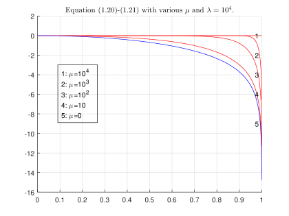
Figure 1: For $\boldsymbol{\lambda}>0$ fixed, equation (1.20)–(1.21) of $v_{\boldsymbol{\mu},\boldsymbol{\lambda}}$ approximates equation (1.5)–(1.6) of $u_{\boldsymbol{\lambda}}$ as $\boldsymbol{\mu}$ tends to zero. Given $\boldsymbol{\lambda}=10^{4}$, the curve 1–5 are associated with $\boldsymbol{\mu}=10^{4},10^{3},10^{2},10,0$, respectively. Note that the curve 1 presents the neutrality ($\boldsymbol{\mu}=\boldsymbol{\lambda}=10^{4}$), which implies $v_{\boldsymbol{\mu},\boldsymbol{\lambda}}\equiv 0$.

Setting $w_{\boldsymbol{\mu},\boldsymbol{\lambda}}:=v_{\boldsymbol{\mu},\boldsymbol{\lambda}}-u_{\boldsymbol{\lambda}}$, we obtain

$$w_{\boldsymbol{\mu},\boldsymbol{\lambda}}^{\prime\prime}\left(r\right)=e^{-v_{\boldsymbol{\mu},\boldsymbol{\lambda}}(r)}W_{\boldsymbol{\mu},\boldsymbol{\lambda}}(r)\,\,\text{with}\,\,W_{\boldsymbol{\mu},\boldsymbol{\lambda}}(r)=\frac{\boldsymbol{\mu}e^{2v_{{\boldsymbol{\mu}},\boldsymbol{\lambda}}(r)}}{\int_{0}^{1}e^{v_{\boldsymbol{\mu},\boldsymbol{\lambda}}(s)}\mathrm{d}s}-\frac{\boldsymbol{\lambda}}{\int_{0}^{1}e^{-v_{\boldsymbol{\mu},\boldsymbol{\lambda}}(s)}\mathrm{d}s}+\frac{\boldsymbol{\lambda}e^{w_{\boldsymbol{\mu},\boldsymbol{\lambda}}(r)}}{\int_{0}^{1}e^{-u_{\boldsymbol{\lambda}}(s)}\mathrm{d}s}.$$

We shall briefly sketch the proof of Theorem 1.1 as follows.

• The basic properties of $v_{\boldsymbol{\mu},\boldsymbol{\lambda}}$ and $w_{\boldsymbol{\lambda}}$ will be stated in Section 4.1. Furthermore, in Lemma 4.2 we carefully deal with $W_{\boldsymbol{\mu},\boldsymbol{\lambda}}$ for the case $\boldsymbol{\lambda}>\boldsymbol{\mu}>0$, and show that $w_{\boldsymbol{\mu},\boldsymbol{\lambda}}$ has neither local maximum nor local minimum in $(0,1)$. Along with $w_{\boldsymbol{\mu},\boldsymbol{\lambda}}^{\prime}(1)=v_{\boldsymbol{\mu},\boldsymbol{\lambda}}^{\prime}(1)-u_{\boldsymbol{\lambda}}^{\prime}(1)=\boldsymbol{\mu}>0$, this particularly shows the monotonic increase of $w_{\boldsymbol{\mu},\boldsymbol{\lambda}}$ with $r$.

• A significant idea for proving Theorem 1.1(a) and (b) is to establish the following estimates:

  • For $w_{\boldsymbol{\mu},\boldsymbol{\lambda}}$, we obtain

    $$0\leq\max_{\left[0,1\right]}{w_{\boldsymbol{\mu},\boldsymbol{\lambda}}}={w_{\boldsymbol{\mu},\boldsymbol{\lambda}}(1)}<\log\bigg{(}\left(1-\frac{\boldsymbol{\mu}}{\boldsymbol{\lambda}}\right)^{2}+\boldsymbol{\mu}\boldsymbol{\lambda}\underbrace{\left(2-\frac{\boldsymbol{\mu}}{\boldsymbol{\lambda}}\right)\frac{e^{-u_{\boldsymbol{\lambda}}(1)}}{\boldsymbol{\lambda}^{2}}}_{\mathop{\text{uniformly\,\,bounded}}\limits_{\mbox{\scriptsize\text{as}\,\,$\boldsymbol{\lambda}\to\infty$}}}\bigg{)}\,\,\underset{\boldsymbol{\mu}\boldsymbol{\lambda}\to 0}{\overset{\boldsymbol{\lambda}\,\,\text{fixed\,\,or}\,\,\boldsymbol{\lambda}\to\infty}{-\!\!\!-\!\!\!-\!\!\!-\!\!\!-\!\!\!-\!\!\!-\!\!\!-\!\!\!-\!\!\!-\!\!\!-\!\!\!\rightarrow}}0$$ (1.26)

    (cf. (4.14)–(4.15) for $\boldsymbol{\lambda}\to\infty$; (4.21) for $\boldsymbol{\lambda}>0$ fixed). Here we shall stress that in (1.26), the condition (1.25) seems optimal since $\displaystyle\lim_{\boldsymbol{\lambda}\to\infty}\textstyle\frac{e^{-u_{\boldsymbol{\lambda}}(1)}}{\boldsymbol{\lambda}^{2}}=\pi^{-2}$ (see (2.5)).

  • For $w_{\boldsymbol{\mu},\boldsymbol{\lambda}}^{\prime}$, we obtain

    $$\max_{\left[0,1\right]}w_{\boldsymbol{\mu},\boldsymbol{\lambda}}^{\prime 2}:=w_{\boldsymbol{\mu},\boldsymbol{\lambda}}^{\prime 2}(r_{\boldsymbol{\mu},\boldsymbol{\lambda}}^{*})\leq \,-\frac{\boldsymbol{\mu}(2e^{v_{\boldsymbol{\mu},\boldsymbol{\lambda}}(r_{\boldsymbol{\mu},\boldsymbol{\lambda}}^{*})}-1)}{\int_{0}^{1}e^{v_{\boldsymbol{\mu},\boldsymbol{\lambda}}(s)}\mathrm{d}s}$$

    $$\,+\boldsymbol{\lambda}\left(\frac{1}{\int_{0}^{1}e^{-v_{\boldsymbol{\mu},\boldsymbol{\lambda}}(s)}\mathrm{d}s}-\frac{1}{\int_{0}^{1}e^{-u_{\boldsymbol{\lambda}}(s)}\mathrm{d}s}\right)\underset{\boldsymbol{\mu}\boldsymbol{\lambda}\to 0}{\overset{\boldsymbol{\lambda}\,\,\text{fixed\,\,or}\,\,\boldsymbol{\lambda}\to\infty}{-\!\!\!-\!\!\!-\!\!\!-\!\!\!-\!\!\!-\!\!\!-\!\!\!-\!\!\!-\!\!\!-\!\!\!-\!\!\!\rightarrow}}0$$

    (cf. (4.19) and Lemma 4.4 for $\boldsymbol{\lambda}\to\infty$; (4.24)–(4.25) for $\boldsymbol{\lambda}>0$ fixed).

Consequently, we obtain $\displaystyle\lim_{\mathop{\boldsymbol{\lambda}\,\,\text{fixed\,\,or}\,\,\boldsymbol{\lambda}\to\infty}\limits_{\mbox{\scriptsize$\boldsymbol{\mu}\boldsymbol{\lambda}\to 0$}}}\left\|w_{\boldsymbol{\mu},\boldsymbol{\lambda}}\right\|_{\mathcal{C}^{1}([0,1])}=0$. The detailed proof of Theorem 1.1 will be stated in Sections 4.2–4.4.

In Theorems 2.1–2.2 below, we will establish the refined far-field and near-field expansions for $u_{\boldsymbol{\lambda}}$ with respect to $\boldsymbol{\lambda}\gg 1$. Combining Theorem 1.1(a) with Theorems 2.1–2.2, we can obtain refined asymptotic expansions of $v_{\boldsymbol{\mu},\boldsymbol{\lambda}}$ as $\boldsymbol{\lambda}\gg 1$ and $0<\boldsymbol{\mu}\boldsymbol{\lambda}\ll 1$. Various asymptotics of $v_{{\boldsymbol{\mu}},\boldsymbol{\lambda}}$ and $u_{\boldsymbol{\lambda}}$ can be presented as follows.

Organization of the paper. The rest of the paper is organized as follows. In Section 2 we will state the main results about the far-field expansions and the near-field expansions of $u_{\boldsymbol{\lambda}}$ in Theorems 2.1 and 2.2, respectively. Based on such asymptotic expansions, we establish in Corollary 2.3 for the refined asymptotic expansions of $\rho_{\boldsymbol{\lambda}}$ and the related concentration phenomenon of $\frac{\rho_{\boldsymbol{\lambda}}}{\boldsymbol{\lambda}}$ as $\boldsymbol{\lambda}\to\infty$. Afterwards, we prove Theorems 2.1–2.2 and Corollary 2.3 in Section 3. We shall stress that Theorem 2.2 plays a crucial role in the proof of Theorem 1.1. In Section 4.1 we introduce some basic properties of $v_{\boldsymbol{\mu},\boldsymbol{\lambda}}$. For Theorem 1.1, we will state the proof of (a) in Sections 4.2–4.3 and the proof of (b) in Section 4.4. Finally, we provide an application to calculating the capacitances and discuss such result in Section 5.

2 The main results of (1.5)–(1.6)

Throughout the whole paper, we denote $o_{\boldsymbol{\lambda}}$ as the quantity tending to zero as $\boldsymbol{\lambda}$ goes to infinity. We are now in a position to state the main results about the far-field and near-field expansions of the solution to (1.5)–(1.6) as follows.

Theorem 2.1 (Far-field expansions of $u_{\boldsymbol{\lambda}}$).

For $\boldsymbol{\lambda}>0$, let $u_{\boldsymbol{\lambda}}\in\mathcal{C}^{2}([0,1])$ be the unique solution to (1.5)–(1.6). Then as $\boldsymbol{\lambda}\gg 1$,

$$\int_{0}^{1}e^{-u_{\boldsymbol{\lambda}}(s)}\mathrm{d}s=\frac{2}{\pi^{2}}\left(\boldsymbol{\lambda}+4+\frac{4}{\boldsymbol{\lambda}}\left(1+o_{\boldsymbol{\lambda}}\right)\right)\to\infty.$$ (2.1)

Moreover, for any compact subset $K$ of $[0,1)$, there holds

$$\boldsymbol{\lambda}^{2}\left\|u_{\boldsymbol{\lambda}}(r)-U(r)-\pi{r}\left(\frac{\sin({\pi}r)}{\boldsymbol{\lambda}}-\frac{\pi{r}+2\sin({\pi}r)}{\boldsymbol{\lambda}^{2}}\right)\sec^{2}\left(\frac{\pi}{2}r\right)\right\|_{\mathcal{C}^{1}(K)}\stackrel{{\scriptstyle\boldsymbol{\lambda}\to\infty}}{{-\!\!\!-\!\!\!-\!\!\!\rightarrow}}0,$$ (2.2)

where $U(r)=2\log\cos\left(\frac{\pi}{2}r\right)$ is the unique solution to (1.12) and $\left\|\,\cdot\,\right\|_{\mathcal{C}^{1}(K)}$ is defined in (1.15).

Remark 1.

(2.2) gives the precise first three terms of $u_{\boldsymbol{\lambda}}(r)$ and $u_{\boldsymbol{\lambda}}^{\prime}(r)$ with respect to $\boldsymbol{\lambda}\gg 1$, for $r\in[0,1)$:

$$u_{\boldsymbol{\lambda}}(r)=U(r)+\pi r\left(\frac{\sin(\pi r)}{\boldsymbol{\lambda}}-\frac{\pi r+2\sin(\pi r)}{\boldsymbol{\lambda}^{2}}\right)\sec^{2}\left(\frac{\pi}{2}r\right)+O\left(\frac{1}{\boldsymbol{\lambda}^{3}}\right),$$ (2.3)

$$u^{\prime}_{\boldsymbol{\lambda}}=U^{\prime}(r)+\frac{2\pi\tan(\pi r/2)+\pi^{2}r\sec^{2}(\pi r/2)}{\boldsymbol{\lambda}}$$

$$\qquad-\frac{4\pi\tan(\pi r/2)+4\pi^{2}r\sec^{2}(\pi r/2)+\pi^{3}r^{2}\sec^{2}(\pi r/2)\tan(\pi r/2)}{\boldsymbol{\lambda}^{2}}+O\left(\frac{1}{\boldsymbol{\lambda}^{3}}\right)$$

In particular, one obtains

$$\lim_{\boldsymbol{\lambda}\to\infty}u_{\boldsymbol{\lambda}}(r)=U(r)\text{ and }~{}\lim_{\boldsymbol{\lambda}\to\infty}u_{\boldsymbol{\lambda}}^{\prime}(r)=U^{\prime}(r)=-\pi\tan\left(\frac{\pi}{2}r\right).$$ (2.4)

We stress that (2.4) can be derived directly from [2]. However, the argument in [2] seems difficult to establish (2.3) due to the lack of (3.3).

Theorem 2.2 (Near-field expansions of $u_{\boldsymbol{\lambda}}$).

Under the same hypotheses as in Theorem 2.1, as $\boldsymbol{\lambda}\gg 1$, we have

$$u_{\boldsymbol{\lambda}}(1)=2\log\frac{1}{\boldsymbol{\lambda}}+2\log\pi-\frac{4}{\boldsymbol{\lambda}}(1+o_{\boldsymbol{\lambda}}).$$ (2.5)

Moreover, for $\alpha,~{}p>0$ independent of $\boldsymbol{\lambda}$, $u_{\boldsymbol{\lambda}}(r_{p,\alpha}^{\boldsymbol{\lambda}})$ asymptotically blows up, which is depicted as follows:

1. If $\alpha>2$, i.e., $\boldsymbol{\lambda}^{2}\mathrm{dist}(r_{p,\alpha}^{\boldsymbol{\lambda}},1)\to 0$, then $u_{\boldsymbol{\lambda}}\left(r_{p,\alpha}^{\boldsymbol{\lambda}}\right)=-2\log\boldsymbol{\lambda}+2\log\pi-\frac{4}{\boldsymbol{\lambda}}(1+o_{\boldsymbol{\lambda}})$, which shares the same first three terms with $u_{\boldsymbol{\lambda}}(1)$, and $u_{\boldsymbol{\lambda}}^{\prime}(r_{p,\alpha}^{\boldsymbol{\lambda}})$ and $u_{\boldsymbol{\lambda}}^{\prime}(1)$ shares the same leading order term, which asymptotically blows up. In particular, $\left|u_{\boldsymbol{\lambda}}^{\prime}(r_{p,\alpha}^{\boldsymbol{\lambda}})-u_{\boldsymbol{\lambda}}^{\prime}(1)\right|\to 0$ as $\boldsymbol{\lambda}\to\infty$.

2. If $1<\alpha\leq 2$, then

   1. $u_{\boldsymbol{\lambda}}(r_{p,\alpha}^{\boldsymbol{\lambda}})$ and $u_{\boldsymbol{\lambda}}(1)$ share the same first two terms:

      $$u_{\boldsymbol{\lambda}}(r_{p,\alpha}^{\boldsymbol{\lambda}})=2\log\frac{1}{\boldsymbol{\lambda}}+2\log\pi+\begin{cases}\displaystyle\frac{p-4}{\boldsymbol{\lambda}}\left(1+o_{\boldsymbol{\lambda}}\right)&\mbox{if }\alpha=2,\\[8.53581pt] \displaystyle\frac{p}{\boldsymbol{\lambda}^{\alpha-1}}\left(1+o_{\boldsymbol{\lambda}}\right)&\mbox{if }\alpha\in\left(1,2\right).\end{cases}$$ (2.6)

   2. $u_{\boldsymbol{\lambda}}^{\prime}(r_{p,\alpha}^{\boldsymbol{\lambda}})$ and $u_{\boldsymbol{\lambda}}^{\prime}(1)$ share the same leading order term:

      $$u_{\boldsymbol{\lambda}}^{\prime}(r_{p,\alpha}^{\boldsymbol{\lambda}})=-\boldsymbol{\lambda}+\frac{p}{2}\boldsymbol{\lambda}^{2-\alpha}(1+o_{\boldsymbol{\lambda}}),\quad\alpha\in(1,2].$$ (2.7)

   Hence, the effect of $p$ and $\alpha$ occurs at the third order term of $u_{\boldsymbol{\lambda}}(r_{p,\alpha}^{\boldsymbol{\lambda}})$ and the second order term $u_{\boldsymbol{\lambda}}^{\prime}(r_{p,\alpha}^{\boldsymbol{\lambda}})$.

3. If $\alpha=1$, then

   1. $u_{\boldsymbol{\lambda}}(r_{p,\alpha}^{\boldsymbol{\lambda}})$ and $u_{\boldsymbol{\lambda}}(1)$ share the same leading order terms:

      $$u_{\boldsymbol{\lambda}}(r_{p,\alpha}^{\boldsymbol{\lambda}})=2\log\frac{1}{\boldsymbol{\lambda}}+2\log\frac{\left(p+2\right)\pi}{2}-\frac{4}{\boldsymbol{\lambda}}\left(1+o_{\boldsymbol{\lambda}}\right).$$ (2.8)

   2. The leading order term of $u_{\boldsymbol{\lambda}}^{\prime}(r_{p,\alpha}^{\boldsymbol{\lambda}})$ depends on $p$:

      $$u_{\boldsymbol{\lambda}}^{\prime}(r_{p,\alpha}^{\boldsymbol{\lambda}})=-\frac{2}{p+2}\boldsymbol{\lambda}+o_{\boldsymbol{\lambda}}.$$ (2.9)

   Hence, the effect of $p$ occurs at the second order term of $u_{\boldsymbol{\lambda}}(r_{p,\alpha}^{\boldsymbol{\lambda}})$ and the leading order term of $u_{\boldsymbol{\lambda}}^{\prime}(r_{p,\alpha}^{\boldsymbol{\lambda}})$.

4. If $0<\alpha<1$, then

   1. The leading order term of $u_{\boldsymbol{\lambda}}(r_{p,\alpha}^{\boldsymbol{\lambda}})$ depends on $\alpha$ and second order term depends on $p$:

      $$u_{\boldsymbol{\lambda}}(r_{p,\alpha}^{\boldsymbol{\lambda}})={2\alpha}\log\frac{1}{\boldsymbol{\lambda}}+2\log\frac{p\pi}{2}+o_{\boldsymbol{\lambda}}.$$ (2.10)

   2. The leading order term of $u_{\boldsymbol{\lambda}}^{\prime}(r_{p,\alpha}^{\boldsymbol{\lambda}})$ depends on $p$ and $\alpha$:

      $$u_{\boldsymbol{\lambda}}^{\prime}(r_{p,\alpha}^{\boldsymbol{\lambda}})=-\frac{2}{p}\boldsymbol{\lambda}^{\alpha}+o_{\boldsymbol{\lambda}}.$$ (2.11)

Thanks to Theorems 2.1 and 2.2, we are able to obtain the pointwise asymptotics of $\boldsymbol{\lambda}^{-1}\rho_{\boldsymbol{\lambda}}$. Moreover, we have (cf. (2.12) and (2.13)) that as $\boldsymbol{\lambda}\gg 1$:

• For $0<\alpha<1/2$, $\displaystyle\sup_{[0,r_{p,\alpha}^{\boldsymbol{\lambda}}]}\boldsymbol{\lambda}^{-1}\rho_{\boldsymbol{\lambda}}$ and $\displaystyle\sup_{[0,r_{p,\alpha}^{\boldsymbol{\lambda}}]}\boldsymbol{\lambda}^{-1}u_{\boldsymbol{\lambda}}^{\prime 2}$ tend to zero.

• For $\alpha=1/2$, $\boldsymbol{\lambda}^{-1}\rho_{\boldsymbol{\lambda}}(r_{p,\alpha}^{\boldsymbol{\lambda}})$ and $\boldsymbol{\lambda}^{-1}u_{\boldsymbol{\lambda}}^{\prime 2}(r_{p,\alpha}^{\boldsymbol{\lambda}})$ are bounded and have positive lower bound.

• For $\alpha>1/2$, $\boldsymbol{\lambda}^{-1}\rho_{\boldsymbol{\lambda}}(r_{p,\alpha}^{\boldsymbol{\lambda}})$ and $\boldsymbol{\lambda}^{-1}u_{\boldsymbol{\lambda}}^{\prime 2}(r_{p,\alpha}^{\boldsymbol{\lambda}})$ asymptotically blow up.

More precisely, we obtain the refined far-field and near-field expansions of the net charge density $\rho_{\boldsymbol{\lambda}}$ and the boundary concentration phenomena of $\boldsymbol{\lambda}^{-1}\rho_{\boldsymbol{\lambda}}$ and $\boldsymbol{\lambda}^{-1}u_{\boldsymbol{\lambda}}^{\prime 2}$, which are stated as follows.

Corollary 2.3.

Under the same hypotheses as in Theorem 2.1, as $\boldsymbol{\lambda}$ approaches infinity, we have

1. (Far-field expansions of $\rho_{\boldsymbol{\lambda}}$) For any compact subset $K$ (independent of $\boldsymbol{\lambda}$) of $[0,1)$,

   $$\rho_{\boldsymbol{\lambda}}(r)=\frac{\pi^{2}}{2}\sec^{2}\left(\frac{\pi}{2}r\right)-\frac{1}{\boldsymbol{\lambda}}\left[2\pi^{2}\sec^{2}\left(\frac{\pi}{2}r\right)+\pi^{3}\sec^{2}\left(\frac{\pi}{2}r\right)\tan\left(\frac{\pi}{2}r\right)\right](1+o_{\boldsymbol{\lambda}})$$ (2.12)

   uniformly in $K$.

2. (Near-field expansions of $\rho_{\boldsymbol{\lambda}}$) The asymptotics of $\rho_{\boldsymbol{\lambda}}$ near the boundary is depicted as follows:

   $$\rho_{\boldsymbol{\lambda}}(r_{p,\alpha}^{\boldsymbol{\lambda}})=\begin{cases}\displaystyle\frac{\boldsymbol{\lambda}^{2}}{2}(1+o_{\boldsymbol{\lambda}})&\mbox{if }\alpha\in(1,\infty),\\[8.53581pt] \displaystyle\frac{2\boldsymbol{\lambda}^{2}}{(p+2)^{2}}(1+o_{\boldsymbol{\lambda}})&\mbox{if }\alpha=1,\\[8.53581pt] \displaystyle\frac{2\boldsymbol{\lambda}^{2\alpha}}{p^{2}}(1+o_{\boldsymbol{\lambda}})&\mbox{if }\alpha\in(0,1).\end{cases}$$ (2.13)

3. (Concentration phenomenon) Both $\boldsymbol{\lambda}^{-1}\rho_{\boldsymbol{\lambda}}$ and $(2\boldsymbol{\lambda})^{-1}u_{\boldsymbol{\lambda}}^{\prime 2}$ behave exactly as Dirac measures supported at boundary point $r=1$, i.e.,

   $$\lim_{\boldsymbol{\lambda}\to\infty}\int_{0}^{1}\frac{\rho_{\boldsymbol{\lambda}}(r)}{\boldsymbol{\lambda}}h(r)\mathrm{d}r =h(1),$$ (2.14)

   $$\lim_{\boldsymbol{\lambda}\to\infty}\int_{0}^{1}\frac{u_{\boldsymbol{\lambda}}^{\prime 2}(r)}{2\boldsymbol{\lambda}}h(r)\mathrm{d}r =h(1),$$ (2.15)

   for any continuous function $h:[0,1]\to\mathbb{R}$ independent of $\boldsymbol{\lambda}$.

3 Proof of Theorems 2.1–2.2 and Corollary 2.3

It is well-known (cf. [2, Appendix]) that $u_{\boldsymbol{\lambda}}$ and $\rho_{\boldsymbol{\lambda}}$ can be expressed as

$$u_{\boldsymbol{\lambda}}(r)=2\log\cos\left(\sqrt{\frac{J_{\boldsymbol{\lambda}}}{2}}r\right)~{}~{}\mbox{and}~{}~{}\rho_{\boldsymbol{\lambda}}(r)=J_{\boldsymbol{\lambda}}\sec^{2}\left(\sqrt{\frac{J_{\boldsymbol{\lambda}}}{2}}r\right)~{}~{}\text{for}~{}r\in\left[0,1\right],$$ (3.1)

where

$$J_{\boldsymbol{\lambda}}=\frac{\boldsymbol{\lambda}}{I_{\boldsymbol{\lambda}}}<\frac{\pi^{2}}{2},\,\,\,\,\text{and}\,\,\,\,I_{\boldsymbol{\lambda}}=\int_{0}^{1}e^{-u_{\boldsymbol{\lambda}}(s)}\mathrm{d}s.$$ (3.2)

To study the asymptotic behaviour of $u_{\boldsymbol{\lambda}}$, it suffices to establish the refined asymptotic expansions of $I_{\boldsymbol{\lambda}}$ and $J_{\boldsymbol{\lambda}}$ which are stated as follows.

Lemma 3.1.

Under the same hypothesis in Theorem 2.1, we have

$$J_{\boldsymbol{\lambda}}=\pi^{2}\left(\frac{1}{2}-\frac{2}{\boldsymbol{\lambda}}+\frac{6}{\boldsymbol{\lambda}^{2}}-\frac{48-2\pi^{2}}{3\boldsymbol{\lambda}^{3}}(1+o_{\boldsymbol{\lambda}})\right)\,\,as\,\,\boldsymbol{\lambda}\gg 1.$$ (3.3)

The proof of Lemma 3.1 is elementary so we state it in Appendix.

Remark 2.

Since (1.5) has a unique solution $u_{\boldsymbol{\lambda}}$ and corresponds to the nonlinear eigenvalue problem (1.10) with $(U_{\kappa},\kappa)=(u_{\boldsymbol{\lambda}},J_{\boldsymbol{\lambda}})$, this results in $\frac{\boldsymbol{\lambda}}{\int_{0}^{1}e^{-u_{\boldsymbol{\lambda}}(s)}\mathrm{d}s}<\frac{\pi^{2}}{2}$ for any positive $\boldsymbol{\lambda}$. We want to point out that (3.3) implies a squeezed estimate

$$\pi^{2}\left(\frac{1}{2}-\frac{2}{\boldsymbol{\lambda}}+\frac{6-\epsilon}{\boldsymbol{\lambda}^{2}}\right)<\frac{\boldsymbol{\lambda}}{\int_{0}^{1}e^{-u_{\boldsymbol{\lambda}}(s)}\mathrm{d}s}<\pi^{2}\left(\frac{1}{2}-\frac{2}{\boldsymbol{\lambda}}+\frac{6}{\boldsymbol{\lambda}^{2}}\right)\,\,as\,\,\boldsymbol{\lambda}>\boldsymbol{\lambda}(\epsilon),$$

for any sufficiently small $\epsilon>0$, where $\boldsymbol{\lambda}(\epsilon)$ is a positive constant depending on $\epsilon$.

Now, we are in a position to state the proof of Theorem 2.1.

$\mathbf{Proof~{}of~{}Theorem~{}\ref{thm:2.1}}$.

(2.1) follows from (3.3) since we have

$$I_{\boldsymbol{\lambda}}=\frac{\boldsymbol{\lambda}}{J_{\boldsymbol{\lambda}}}=\frac{2\boldsymbol{\lambda}}{\pi^{2}}\left(1-\frac{4}{\boldsymbol{\lambda}}+\frac{12}{\boldsymbol{\lambda}^{2}}(1+o_{\boldsymbol{\lambda}})\right)^{-1}=\frac{2}{\pi^{2}}\left(\boldsymbol{\lambda}+4+\frac{4}{\boldsymbol{\lambda}}(1+o_{\boldsymbol{\lambda}})\right).$$

To prove (2.2), we need to establish the precise first third order terms of $u_{\boldsymbol{\lambda}}(r)$ and $u_{\boldsymbol{\lambda}}^{\prime}(r)$ in $K$. Firstly, by (3.1) and (3.3), there holds that

$$u_{\boldsymbol{\lambda}}(r)=2\log\cos\left(\frac{\pi}{2}r-\frac{\pi}{\boldsymbol{\lambda}}r+\frac{2\pi}{\boldsymbol{\lambda}^{2}}r(1+o_{\boldsymbol{\lambda}})\right)\,\,\mathrm{uniformly\,\,in}\,\,K,\,\,\mathrm{as}\,\,\boldsymbol{\lambda}\to\infty.$$ (3.4)

Note that $r\in K$ is independent of $\boldsymbol{\lambda}$. For a sake of convenience, let us set

$$\xi(r)=-\frac{\pi}{\boldsymbol{\lambda}}r+\frac{2\pi}{\boldsymbol{\lambda}^{2}}r(1+o_{\boldsymbol{\lambda}}).$$ (3.5)

Then, as $\boldsymbol{\lambda}\to\infty$, we have $\xi(r)\to 0$ and

$$2\log\cos\left(\frac{\pi}{2}r+\xi(r)\right)=2\log\cos\left(\frac{\pi}{2}r\right)-2\xi(r)\tan\left(\frac{\pi}{2}r\right)-\xi^{2}(r)\sec^{2}\left(\frac{\pi}{2}r\right)+o(\xi^{3}(r)),$$ (3.6)

uniformly in $K$. (3.6) can be obtained directly from the Taylor expansions so we omit the detailed derivation. As a consequence, by (3.4)–(3.6),

$$u_{\boldsymbol{\lambda}}(r)= 2\log\cos\left(\frac{\pi}{2}r\right)+\frac{2\pi r}{\boldsymbol{\lambda}}\tan\left(\frac{\pi}{2}r\right)-\frac{\pi r}{\boldsymbol{\lambda}^{2}}\left(4\tan\left(\frac{\pi}{2}r\right)+\pi r\sec^{2}\left(\frac{\pi}{2}r\right)\right)(1+o_{\boldsymbol{\lambda}})$$ (3.7)

$$= 2\log\cos\left(\frac{\pi}{2}r\right)+\pi r\sec^{2}\left(\frac{\pi}{2}r\right)\left(\frac{\sin(\pi r)}{\boldsymbol{\lambda}}-\frac{\pi r+2\sin(\pi r)}{\boldsymbol{\lambda}^{2}}\right)(1+o_{\boldsymbol{\lambda}}),$$

which gives the precise first third order terms of $u_{\boldsymbol{\lambda}}(r)$.

On the other hand, differentiating (3.1) to $r$ gives

$$u_{\boldsymbol{\lambda}}^{\prime}(r)=-2\sqrt{\frac{J_{\boldsymbol{\lambda}}}{2}}\tan\left(\sqrt{\frac{J_{\boldsymbol{\lambda}}}{2}}r\right).$$ (3.8)

Hence, by virtue of (3.3), (3.5) and (3.8), an expansion of $u_{\boldsymbol{\lambda}}^{\prime}(r)$ with respect to $\boldsymbol{\lambda}\gg 1$ can be expressed as

$$u_{\boldsymbol{\lambda}}^{\prime}(r)= \left(-\pi+\frac{2\pi}{\boldsymbol{\lambda}}-\frac{4\pi}{\boldsymbol{\lambda}^{2}}(1+o_{\boldsymbol{\lambda}})\right)\tan\left(\frac{\pi}{2}r-\frac{\pi}{\boldsymbol{\lambda}}r+\frac{2\pi}{\boldsymbol{\lambda}^{2}}r(1+o_{\boldsymbol{\lambda}})\right)$$ (3.9)

$$= -\pi\tan\left(\frac{\pi}{2}r\right)+\frac{\pi^{2}r+\pi\sin(\pi r)}{\boldsymbol{\lambda}}\sec^{2}\left(\frac{\pi}{2}r\right)$$

$$-\frac{\pi}{\boldsymbol{\lambda}^{2}}\left[4\tan\left(\frac{\pi}{2}r\right)+4\pi r\sec^{2}\left(\frac{\pi}{2}r\right)+\pi^{2}r^{2}\sec^{2}\left(\frac{\pi}{2}r\right)\tan\left(\frac{\pi}{2}r\right)\right](1+o_{\boldsymbol{\lambda}}),$$

uniformly in $K$. Here we have used the approximation

$$\tan\left(\frac{\pi}{2}r+\xi(r)\right)=\tan\left(\frac{\pi}{2}r\right)+\xi(r)\sec^{2}\left(\frac{\pi}{2}r\right)+\xi^{2}(r)\sec^{2}\left(\frac{\pi}{2}r\right)\tan\left(\frac{\pi}{2}r\right)+o(\xi^{3}(r)).$$

Therefore, (2.2) follows immediately from (3.7) and (3.9), and we complete the proof of Theorem 2.1. ∎

3.1 Proof of Theorem 2.2

(2.5) follows from (1.9) and (3.2)–(3.3). By (3.1) and (3.8), we have

$$u_{\boldsymbol{\lambda}}(r_{p,\alpha}^{\boldsymbol{\lambda}})=2\log\cos\left(r_{p,\alpha}^{\boldsymbol{\lambda}}\sqrt{\frac{J_{\boldsymbol{\lambda}}}{2}}\right)=2\log\sin\left(\frac{\pi}{2}-r_{p,\alpha}^{\boldsymbol{\lambda}}\sqrt{\frac{J_{\boldsymbol{\lambda}}}{2}}\right),$$ (3.10)

and

$$u_{\boldsymbol{\lambda}}^{\prime}(r_{p,\alpha}^{\boldsymbol{\lambda}})=-\sqrt{2J_{\boldsymbol{\lambda}}}\tan\left(r_{p,\alpha}^{\boldsymbol{\lambda}}\sqrt{\frac{J_{\boldsymbol{\lambda}}}{2}}\right),$$ (3.11)

where $r_{p,\alpha}^{\boldsymbol{\lambda}}$ is defined in (1.14). On the other hand, by (1.14) and (3.3), we have

$$r_{p,\alpha}^{\boldsymbol{\lambda}}\sqrt{\frac{J_{\boldsymbol{\lambda}}}{2}}=\left(1-\frac{p}{\boldsymbol{\lambda}^{\alpha}}\right)\left(\frac{\pi}{2}-\frac{\pi}{\boldsymbol{\lambda}}+\frac{2\pi}{\boldsymbol{\lambda}^{2}}(1+o_{\boldsymbol{\lambda}})\right).$$ (3.12)

Note that the asymptotic expansion of $r_{p,\alpha}^{\boldsymbol{\lambda}}\sqrt{J_{\boldsymbol{\lambda}}/2}$ varies with $\alpha$. To obtain the refined asymptotic expansions of (3.10) and (3.11), we shall deal with the asymptotics of $r_{p,\alpha}^{\boldsymbol{\lambda}}\sqrt{J_{\boldsymbol{\lambda}}/2}$ under situations $\alpha>2$, $1<\alpha\leq 2$, $\alpha=1$ and $0<\alpha<1$ individually.

Case 1. $\alpha>2$:

In this case, we have $0<\frac{1}{\boldsymbol{\lambda}^{\alpha}}\ll\frac{1}{\boldsymbol{\lambda}^{2}}$ as $\boldsymbol{\lambda}\gg 1$. Hence,

$$r_{p,\alpha}^{\boldsymbol{\lambda}}\sqrt{\frac{J_{\boldsymbol{\lambda}}}{2}}=\left(1-\frac{p}{\boldsymbol{\lambda}^{\alpha}}\right)\left(\frac{\pi}{2}-\frac{\pi}{\boldsymbol{\lambda}}+\frac{2\pi}{\boldsymbol{\lambda}^{2}}(1+o_{\boldsymbol{\lambda}})\right)=\frac{\pi}{2}-\frac{\pi}{\boldsymbol{\lambda}}+\frac{2\pi}{\boldsymbol{\lambda}^{2}}(1+o_{\boldsymbol{\lambda}}).$$ (3.13)

Along with (3.10), one may make appropriate manipulations to obtain

$$u_{\boldsymbol{\lambda}}\left(r_{p,\alpha}^{\boldsymbol{\lambda}}\right)=\,2\log\sin\left(\frac{\pi}{\boldsymbol{\lambda}}-\frac{2\pi}{\boldsymbol{\lambda}^{2}}(1+o_{\boldsymbol{\lambda}})\right)=\log\frac{1}{\boldsymbol{\lambda}^{2}}+\log\pi^{2}-\frac{4}{\boldsymbol{\lambda}}(1+o_{\boldsymbol{\lambda}}).$$ (3.14)

On the other hand, by (3.11), (3.13) and Taylor expansions of the cotangent function, one may check that

$$u_{\boldsymbol{\lambda}}^{\prime}(r_{p,\alpha}^{\boldsymbol{\lambda}})= \left(-\pi+\frac{2\pi}{\boldsymbol{\lambda}}-\frac{4\pi}{\boldsymbol{\lambda}^{2}}\left(1+o_{\boldsymbol{\lambda}}\right)\right)\tan\left[\left(1-\frac{p}{\boldsymbol{\lambda}^{\alpha}}\right)\left(\frac{\pi}{2}-\frac{\pi}{\boldsymbol{\lambda}}+\frac{2\pi}{\boldsymbol{\lambda}^{2}}\left(1+o_{\boldsymbol{\lambda}}\right)\right)\right]$$ (3.15)

$$= \left(-\pi+\frac{2\pi}{\boldsymbol{\lambda}}-\frac{4\pi}{\boldsymbol{\lambda}^{2}}\left(1+o_{\boldsymbol{\lambda}}\right)\right)\cot\left(\frac{\pi}{\boldsymbol{\lambda}}-\frac{2\pi}{\boldsymbol{\lambda}^{2}}\left(1+o_{\boldsymbol{\lambda}}\right)\right)=-\boldsymbol{\lambda}+o_{\boldsymbol{\lambda}}.$$

Therefore, Theorem 2.2(a) follows from (3.14) and (3.15).

Case 2. $1<\alpha\leq 2$:

In this case, (3.12) gives

$$r_{p,\alpha}^{\boldsymbol{\lambda}}\sqrt{\frac{J_{\boldsymbol{\lambda}}}{2}}=\left(1-\frac{p}{\boldsymbol{\lambda}^{\alpha}}\right)\left(\frac{\pi}{2}-\frac{\pi}{\boldsymbol{\lambda}}+\frac{2\pi}{\boldsymbol{\lambda}^{2}}(1+o_{\boldsymbol{\lambda}})\right)=\frac{\pi}{2}-\frac{\pi}{\boldsymbol{\lambda}}-\frac{p\pi}{2\boldsymbol{\lambda}^{\alpha}}+\frac{2\pi}{\boldsymbol{\lambda}^{2}}(1+o_{\boldsymbol{\lambda}}).$$ (3.16)

Along with (3.10) one obtains

$$u_{\boldsymbol{\lambda}}(r_{p,\alpha}^{\boldsymbol{\lambda}})= 2\log\left(\frac{\pi}{\boldsymbol{\lambda}}+\frac{p\pi}{2\boldsymbol{\lambda}^{\alpha}}-\frac{2\pi}{\boldsymbol{\lambda}^{2}}(1+o_{\boldsymbol{\lambda}})\right)=2\log\frac{\pi}{\boldsymbol{\lambda}}+2\log\left(1+\frac{p}{2\boldsymbol{\lambda}^{\alpha-1}}-\frac{2}{\boldsymbol{\lambda}}(1+o_{\boldsymbol{\lambda}})\right)$$

$$= \log\frac{1}{\boldsymbol{\lambda}^{2}}+\log\pi^{2}+\begin{cases}\displaystyle\frac{p-4}{\boldsymbol{\lambda}}(1+o_{\boldsymbol{\lambda}})&\mbox{if }\alpha=2,\\[8.53581pt] \displaystyle\frac{p}{\boldsymbol{\lambda}^{\alpha-1}}(1+o_{\boldsymbol{\lambda}})&\mbox{if }\alpha\in\left(1,2\right),\end{cases}$$

and (2.6) immediately follows from this result. Combining (3.11) with (3.16) and following similar argument, we get (2.7) and complete the proof of Theorem 2.2(b).

Case 3. $\alpha=1$:

In this case, (3.12) becomes

$$r_{p,\alpha}^{\boldsymbol{\lambda}}\sqrt{\frac{J_{\boldsymbol{\lambda}}}{2}}=\left(1-\frac{p}{\boldsymbol{\lambda}}\right)\left(\frac{\pi}{2}-\frac{\pi}{\boldsymbol{\lambda}}+\frac{2\pi}{\boldsymbol{\lambda}^{2}}(1+o_{\boldsymbol{\lambda}})\right)=\frac{\pi}{2}-\frac{(p+2)\pi}{2\boldsymbol{\lambda}}+\frac{(p+2)\pi}{\boldsymbol{\lambda}^{2}}(1+o_{\boldsymbol{\lambda}}).$$ (3.17)

Hence, by inserting (3.17) into (3.10) and following the similar argument as in (3.14), we obtain

$$u_{\boldsymbol{\lambda}}(r_{p,\alpha}^{\boldsymbol{\lambda}})=2\log\sin\left(\frac{(p+2)\pi}{2\boldsymbol{\lambda}}-\frac{(p+2)\pi}{\boldsymbol{\lambda}^{2}}(1+o_{\boldsymbol{\lambda}})\right)=\log\frac{1}{\boldsymbol{\lambda}^{2}}+\log\frac{(p+2)^{2}\pi^{2}}{4}-\frac{4}{\boldsymbol{\lambda}}(1+o_{\boldsymbol{\lambda}}).$$

This implies (2.8). Finally, (2.9) can be obtained from (3.11) and (3.17). The proof of Theorem 2.2(c) is complete.

Case 4. $0<\alpha<1$:

We want to emphasize that due to $0<\frac{1}{\boldsymbol{\lambda}}\ll\frac{1}{\boldsymbol{\lambda}^{\alpha}}$ as $\boldsymbol{\lambda}\gg 1$, the asymptotics of $u_{\boldsymbol{\lambda}}(r_{p,\alpha}^{\boldsymbol{\lambda}})$ is more complicated than previous three cases.

Firstly, by plugging (3.12) into (3.10), one may obtain

$$u_{\boldsymbol{\lambda}}(r_{p,\alpha}^{\boldsymbol{\lambda}})= \,2\log\sin\left(\frac{p\pi}{2\boldsymbol{\lambda}^{\alpha}}+\frac{\pi}{\boldsymbol{\lambda}}(1+o_{\boldsymbol{\lambda}})\right)$$ (3.18)

$$= \,2\log\left[\left(\frac{p\pi}{2\boldsymbol{\lambda}^{\alpha}}+\frac{\pi}{\boldsymbol{\lambda}}(1+o_{\boldsymbol{\lambda}})\right)-\frac{1}{6}\left(\frac{p\pi}{2\boldsymbol{\lambda}^{\alpha}}+\frac{\pi}{\boldsymbol{\lambda}}(1+o_{\boldsymbol{\lambda}})\right)^{3}(1+o_{\boldsymbol{\lambda}})\right].$$

Note also that $\frac{1}{\boldsymbol{\lambda}^{3\alpha}}\ll\frac{1}{\boldsymbol{\lambda}}$ as $3\alpha>1$, and $\frac{1}{\boldsymbol{\lambda}^{3\alpha}}\gg\frac{1}{\boldsymbol{\lambda}}$ as $0<3\alpha<1$. We shall deal with (3.18) under three situations $0<\alpha<1/3$, $\alpha=1/3$ and $\alpha>1/3$. After simple calculations, we can establish the precise first three terms of $u_{\boldsymbol{\lambda}}(r_{p,\alpha}^{\boldsymbol{\lambda}})$ as follows:

$$u_{\boldsymbol{\lambda}}(r_{p,\alpha}^{\boldsymbol{\lambda}}) =\begin{cases}\displaystyle 2\log\left(\frac{p\pi}{2\boldsymbol{\lambda}^{\alpha}}+\frac{\pi}{\boldsymbol{\lambda}}\left(1+o_{\boldsymbol{\lambda}}\right)\right)&\mbox{if }\alpha\in\left(1/3,1\right),\\[8.53581pt] \displaystyle 2\log\left(\frac{p\pi}{2\boldsymbol{\lambda}^{\alpha}}+\frac{48\pi-p^{3}\pi^{3}}{48\boldsymbol{\lambda}}\left(1+o_{\boldsymbol{\lambda}}\right)\right)&\mbox{if }\alpha=1/3,\\[8.53581pt] \displaystyle 2\log\left(\frac{p\pi}{2\boldsymbol{\lambda}^{\alpha}}-\frac{p^{3}\pi^{3}}{48\boldsymbol{\lambda}^{3\alpha}}\left(1+o_{\boldsymbol{\lambda}}\right)\right)&\mbox{if }\alpha\in\left(0,1/3\right),\end{cases}$$

$$=\log\frac{1}{\boldsymbol{\lambda}^{2\alpha}}+\log\frac{p^{2}\pi^{2}}{4}(1+o_{\boldsymbol{\lambda}}).$$

Thus, we obtain (2.10).

To prove (2.11), we shall deal with the asymptotics of (3.11) with $0<\alpha<1$. The argument is similar as the previous cases. Indeed, by (3.12) one may check that

$$\tan\left(r_{p,\alpha}^{\boldsymbol{\lambda}}\sqrt{\frac{J_{\boldsymbol{\lambda}}}{2}}\right)= \tan\left[\left(1-\frac{p}{\boldsymbol{\lambda}^{\alpha}}\right)\left(\frac{\pi}{2}-\frac{\pi}{\boldsymbol{\lambda}}(1+o_{\boldsymbol{\lambda}})\right)\right]=\cot\left(\frac{p\pi}{2\boldsymbol{\lambda}^{\alpha}}+\frac{\pi}{\boldsymbol{\lambda}}(1+o_{\boldsymbol{\lambda}})\right)$$ (3.19)

$$= \frac{1}{\frac{p\pi}{2\boldsymbol{\lambda}^{\alpha}}+\frac{\pi}{\boldsymbol{\lambda}}(1+o_{\boldsymbol{\lambda}})}=\frac{2\boldsymbol{\lambda}^{\alpha}}{p\pi}+o_{\boldsymbol{\lambda}}.$$

Combining (3.3), (3.11) and (3.19), we obtain

$$u_{\boldsymbol{\lambda}}^{\prime}(r_{p,\alpha}^{\boldsymbol{\lambda}})=\left(-\pi+\frac{2\pi}{\boldsymbol{\lambda}}(1+o_{\boldsymbol{\lambda}})\right)\left(\frac{2\boldsymbol{\lambda}^{\alpha}}{p\pi}+o_{\boldsymbol{\lambda}}\right)=-\frac{2}{p}\boldsymbol{\lambda}^{\alpha}+o_{\boldsymbol{\lambda}}.$$

Therefore, we get (2.11) and complete the proof of Theorem 2.2.

3.2 Proof of Corollary 2.3

(2.12) follows from the combination of (3.1) and (3.3) as follows:

$$\rho_{\boldsymbol{\lambda}}(r)= \left(\frac{\pi^{2}}{2}-\frac{2\pi^{2}}{\boldsymbol{\lambda}}+\frac{6\pi^{2}}{\boldsymbol{\lambda}^{2}}\left(1+o_{\boldsymbol{\lambda}}\right)\right)\sec^{2}\left(\frac{\pi r}{2}-\frac{\pi r}{\boldsymbol{\lambda}}+\frac{2\pi r}{\boldsymbol{\lambda}^{2}}(1+o_{\boldsymbol{\lambda}})\right)$$

$$= \frac{\pi^{2}}{2}\sec^{2}\left(\frac{\pi}{2}r\right)-\frac{1}{\boldsymbol{\lambda}}\left[2\pi^{2}\sec^{2}\left(\frac{\pi}{2}r\right)+\pi^{3}\sec^{2}\left(\frac{\pi}{2}r\right)\tan\left(\frac{\pi}{2}r\right)\right](1+o_{\boldsymbol{\lambda}}),$$

This completes the proof of Corollary 2.3(a).

Now, we shall prove (2.13). Putting $r=r_{p,\alpha}^{\boldsymbol{\lambda}}$ into the expression of $\rho_{\boldsymbol{\lambda}}$ in (3.1) and using (3.3), we can obtain

$$\rho_{\boldsymbol{\lambda}}(r_{p,\alpha}^{\boldsymbol{\lambda}}) =J_{\boldsymbol{\lambda}}\sec^{2}\left(r_{p,\alpha}^{\boldsymbol{\lambda}}\sqrt{\frac{J_{\boldsymbol{\lambda}}}{2}}\right)$$ (3.20)

$$=\left(\frac{\pi^{2}}{2}-\frac{2\pi^{2}}{\boldsymbol{\lambda}}+\frac{6\pi^{2}}{\boldsymbol{\lambda}^{2}}\left(1+o_{\boldsymbol{\lambda}}\right)\right)\sec^{2}\left[\left(\frac{\pi}{2}-\frac{\pi}{\boldsymbol{\lambda}}+\frac{2\pi}{\boldsymbol{\lambda}^{2}}(1+o_{\boldsymbol{\lambda}})\right)\left(1-\frac{p}{\boldsymbol{\lambda}^{\alpha}}\right)\right].$$

Note that the expansion of $\left(\frac{\pi}{2}-\frac{\pi}{\boldsymbol{\lambda}}+\frac{2\pi}{\boldsymbol{\lambda}^{2}}(1+o_{\boldsymbol{\lambda}})\right)\left(1-\frac{p}{\boldsymbol{\lambda}^{\alpha}}\right)$ depends variously on $\alpha\in\left(0,1\right)$, $\alpha=1$ and $\alpha\in\left(1,\infty\right)$. Firstly, we deal with (3.20) for the case of $0<\alpha<1$ and obtain

$$\rho_{\boldsymbol{\lambda}}(r_{p,\alpha}^{\boldsymbol{\lambda}}) =\left(\frac{\pi^{2}}{2}-\frac{2\pi^{2}}{\boldsymbol{\lambda}}+\frac{6\pi^{2}}{\boldsymbol{\lambda}^{2}}(1+o_{\boldsymbol{\lambda}})\right)\sec^{2}\left(\frac{\pi}{2}-\frac{p\pi}{2\boldsymbol{\lambda}^{\alpha}}+\frac{\pi}{\boldsymbol{\lambda}}(1+o_{\boldsymbol{\lambda}})\right)$$

$$=\frac{2\boldsymbol{\lambda}^{2\alpha}}{p^{2}}(1+o_{\boldsymbol{\lambda}}),$$

Here we have used the standard expansion of the cosecant function to obtain the last identity. Hence, we obtain (2.13) for the case of $0<\alpha<1$. By a similar argument, we can also prove (2.13) for the two cases $\alpha=1$ and $\alpha>1$, and the proof of Corollary 2.3(b) is complete.

It remains to prove Corollary 2.3(c). Note that $\displaystyle\lim_{\boldsymbol{\lambda}\to\infty}\frac{1}{\int_{0}^{1}e^{-u_{\boldsymbol{\lambda}}(s)}\mathrm{d}s}=0$ (by (2.1)). Along with (1.5), we arrive at

$$\limsup_{\boldsymbol{\lambda}\to\infty}\left(\frac{\rho_{\boldsymbol{\lambda}}(r)h(r)}{\boldsymbol{\lambda}}-\frac{u_{\boldsymbol{\lambda}}^{\prime 2}(r)h(r)}{2\boldsymbol{\lambda}}\right)=\lim_{\boldsymbol{\lambda}\to\infty}\frac{h(r)}{\int_{0}^{1}e^{-u_{\boldsymbol{\lambda}}(s)}\mathrm{d}s}=0~{}~{}\mbox{uniformly~{}on~{}}\left[0,1\right]~{}\mbox{as}~{}\boldsymbol{\lambda}\to\infty,$$

where $h$ is a continuous function on $\left[0,1\right]$. This indicates that (2.14) and (2.15) are equivalent. Hence, it suffices to claim (2.14), i.e.,

$$\lim_{\boldsymbol{\lambda}\to\infty}\int_{0}^{1}\frac{e^{-u_{\boldsymbol{\lambda}}(r)}h(r)}{\int_{0}^{1}e^{-u_{\boldsymbol{\lambda}}(s)}\mathrm{d}s}\mathrm{d}r=h(1).$$ (3.21)

Let $\kappa\in(0,1)$ be fixed. Then we observe that

$$\left|\int_{0}^{1}\frac{e^{-u_{\boldsymbol{\lambda}}(r)}}{\int_{0}^{1}e^{-u_{\boldsymbol{\lambda}}(s)}\mathrm{d}s}h(r)\mathrm{d}r-h(1)\right| =\left|\left(\int_{0}^{1-\boldsymbol{\lambda}^{-\kappa}}+\int_{1-\boldsymbol{\lambda}^{-\kappa}}^{1}\right)\frac{e^{-u_{\boldsymbol{\lambda}}(r)}}{\int_{0}^{1}e^{-u_{\boldsymbol{\lambda}}(s)}\mathrm{d}s}(h(r)-h(1))\mathrm{d}r\right|$$ (3.22)

$$\leq 2\max_{r\in[0,1]}|h(r)|\left(\int_{0}^{1-\boldsymbol{\lambda}^{-\kappa}}\frac{e^{-u_{\boldsymbol{\lambda}}(r)}}{\int_{0}^{1}e^{-u_{\boldsymbol{\lambda}}(s)}\mathrm{d}s}\mathrm{d}r\right)$$

$$~{}~{}~{}+\max_{r\in[1-\boldsymbol{\lambda}^{-\kappa},1]}|h(r)-h(1)|\left(\int_{1-\boldsymbol{\lambda}^{-\kappa}}^{1}\frac{e^{-u_{\boldsymbol{\lambda}}(r)}}{\int_{0}^{1}e^{-u_{\boldsymbol{\lambda}}(s)}\mathrm{d}s}\mathrm{d}r\right).$$

Moreover, from (1.5) and Theorem 2.1(d), a direct computation gives

$$\lim_{\boldsymbol{\lambda}\to\infty}\int_{1-\boldsymbol{\lambda}^{-\kappa}}^{1}\frac{e^{-u_{\boldsymbol{\lambda}}(r)}}{\int_{0}^{1}e^{-u_{\boldsymbol{\lambda}}(s)}\mathrm{d}s}\mathrm{d}r=-\lim_{\boldsymbol{\lambda}\to\infty}\int_{1-\boldsymbol{\lambda}^{-\kappa}}^{1}\frac{u_{\boldsymbol{\lambda}}^{\prime\prime}(r)}{\boldsymbol{\lambda}}\mathrm{d}r=\lim_{\boldsymbol{\lambda}\to\infty}\frac{u_{\boldsymbol{\lambda}}^{\prime}(1-\boldsymbol{\lambda}^{-\kappa})-u_{\boldsymbol{\lambda}}^{\prime}(1)}{\boldsymbol{\lambda}}=1,$$

which also implies

$$\lim_{\boldsymbol{\lambda}\to\infty}\int_{0}^{1-{\boldsymbol{\lambda}}^{-\kappa}}\frac{e^{-u_{\boldsymbol{\lambda}}(r)}}{\int_{0}^{1}e^{-u_{\boldsymbol{\lambda}}(s)}\mathrm{d}s}\mathrm{d}r=0.$$ (3.23)

Finally, we notice that the continuity of $h$ implies $\displaystyle\lim_{\boldsymbol{\lambda}\to\infty}\max_{r\in\left[1-{\boldsymbol{\lambda}}^{-\kappa},1\right]}|h(r)-h(1)|=0$. As a consequence, (3.21) immediately follows (3.22)–(3.23) and we prove Corollary 2.3(c).

Therefore, the proof of Corollary 2.3 is completed.

4 Proof of Theorem 1.1

In order to deal with the convergence of the $v_{\boldsymbol{\mu},\boldsymbol{\lambda}}-u_{\boldsymbol{\lambda}}$ with respect to $\boldsymbol{\mu}\boldsymbol{\lambda}\to 0^{+}$, throughout the whole section we shall set

$$w_{\boldsymbol{\mu},\boldsymbol{\lambda}}:=v_{\boldsymbol{\mu},\boldsymbol{\lambda}}-u_{\boldsymbol{\lambda}}.$$ (4.1)

Subtracting (1.5) from (1.20) and using (4.1) gives

$$w_{\boldsymbol{\mu},\boldsymbol{\lambda}}^{\prime\prime}\left(r\right)=\frac{\boldsymbol{\mu}e^{v_{\boldsymbol{\mu},\boldsymbol{\lambda}}(r)}}{\int_{0}^{1}e^{v_{\boldsymbol{\mu},\boldsymbol{\lambda}}(s)}\mathrm{d}s}+\boldsymbol{\lambda}\left(\frac{e^{-u_{\boldsymbol{\lambda}}(r)}}{\int_{0}^{1}e^{-u_{\boldsymbol{\lambda}}(s)}\mathrm{d}s}-\frac{e^{-v_{\boldsymbol{\mu},\boldsymbol{\lambda}}(r)}}{\int_{0}^{1}e^{-v_{\boldsymbol{\mu},\boldsymbol{\lambda}}(s)}\mathrm{d}s}\right)$$ (4.2)

and

$$w_{\boldsymbol{\mu},\boldsymbol{\lambda}}^{\prime\prime}(r)=e^{-v_{\boldsymbol{\mu},\boldsymbol{\lambda}}(r)}\left(\frac{\boldsymbol{\mu}e^{2v_{{\boldsymbol{\mu}},\boldsymbol{\lambda}}(r)}}{\int_{0}^{1}e^{v_{\boldsymbol{\mu},\boldsymbol{\lambda}}(s)}\mathrm{d}s}-\frac{\boldsymbol{\lambda}}{\int_{0}^{1}e^{-v_{\boldsymbol{\mu},\boldsymbol{\lambda}}(s)}\mathrm{d}s}+\frac{\boldsymbol{\lambda}e^{w_{\boldsymbol{\mu},\boldsymbol{\lambda}}(r)}}{\int_{0}^{1}e^{-u_{\boldsymbol{\lambda}}(s)}\mathrm{d}s}\right).$$ (4.3)

We will sometimes use identity (4.2) or identity (4.3) to estimate $w_{\boldsymbol{\mu},\boldsymbol{\lambda}}$ and $w_{\boldsymbol{\mu},\boldsymbol{\lambda}}^{\prime}$ for a sake of convenience.

Since we know that both $u_{\boldsymbol{\lambda}}$ and $v_{\boldsymbol{\mu},\boldsymbol{\lambda}}$ are strictly decreasing on $[0,1]$ (by Lemma 4.1), the main difficulty of Theorem 1.1 is to obtain the monotonicity of $w_{\boldsymbol{\mu},\boldsymbol{\lambda}}$, which will be presented in Lemma 4.2. To complete the proof of Theorem 1.1(a), in Sections 4.2 and 4.3, we will prove

$$\lim_{\mathop{\boldsymbol{\lambda}\to\infty}\limits_{\mbox{\scriptsize$\boldsymbol{\mu}\boldsymbol{\lambda}\to 0$}}}\max_{\left[0,1\right]}\left|w_{\boldsymbol{\mu},\boldsymbol{\lambda}}\right|=0$$ (4.4)

and

$$\lim_{\mathop{\boldsymbol{\lambda}\to\infty}\limits_{\mbox{\scriptsize$\boldsymbol{\mu}\boldsymbol{\lambda}\to 0$}}}\max_{\left[0,1\right]}\left|w_{\boldsymbol{\mu},\boldsymbol{\lambda}}^{\prime}\right|=0,$$ (4.5)

respectively. When $\boldsymbol{\lambda}>0$ is fixed and $\boldsymbol{\mu}\to 0^{+}$, the proof of Theorem 1.1(b) is based on preliminary estimates in Section 4.1–4.3. We will briefly state the proof in section 4.4.

4.1 Some basic properties

Since $\boldsymbol{\lambda}>\boldsymbol{\mu}>0$, one can follow the same argument as in [26, Lemma 2.1] and [28, Proposition 2.1] to obtain $v_{\boldsymbol{\mu},\boldsymbol{\lambda}}^{\prime\prime}(r)=\frac{\boldsymbol{\mu}e^{v_{\boldsymbol{\mu},\boldsymbol{\lambda}}(r)}}{\int_{0}^{1}e^{v_{\boldsymbol{\mu},\boldsymbol{\lambda}}(s)}\text{d}s}-\frac{\boldsymbol{\lambda}e^{-v_{\boldsymbol{\mu},\boldsymbol{\lambda}}(r)}}{\int_{0}^{1}e^{-v_{\boldsymbol{\mu},\boldsymbol{\lambda}}(s)}\text{d}s}<0$ for all $r\in(0,1]$. Along with (1.21), it yields

$$v_{\boldsymbol{\mu},\boldsymbol{\lambda}}^{\prime}(r)<v_{\boldsymbol{\mu},\boldsymbol{\lambda}}^{\prime}(0)=0~{}\text{and}~{}v_{\boldsymbol{\mu},\boldsymbol{\lambda}}(r)<v_{\boldsymbol{\mu},\boldsymbol{\lambda}}(0)=0~{}\text{for all}~{}r\in(0,1].$$

As a consequence, we obtain the following property.

Lemma 4.1.

For $\boldsymbol{\lambda}>\boldsymbol{\mu}>0$, let $v_{\boldsymbol{\mu},\boldsymbol{\lambda}}\in\mathcal{C}^{2}([0,1])$ be the unique solution to (1.20)–(1.21). Then $v_{\boldsymbol{\mu},\boldsymbol{\lambda}}$ is strictly decreasing and strictly concave downward on $\left[0,1\right]$.

Lemma 4.1 and (1.8) present that $v_{\boldsymbol{\mu},\boldsymbol{\lambda}}$ and $u_{\boldsymbol{\lambda}}$ are strictly decreasing on $[0,1]$, but do not provide further information for $w_{\boldsymbol{\mu},\boldsymbol{\lambda}}:=v_{\boldsymbol{\mu},\boldsymbol{\lambda}}-u_{\boldsymbol{\lambda}}$. To prove (4.4), we need two crucial lemmas. Firstly, we obtain that $v_{\boldsymbol{\mu},\boldsymbol{\lambda}}>u_{\boldsymbol{\lambda}}$ on $\left(0,1\right]$ and $w_{\boldsymbol{\mu},\boldsymbol{\lambda}}$ is monotonically increasing as $\boldsymbol{\lambda}>\boldsymbol{\mu}>0$, which is stated as follows.

Lemma 4.2.

For $0<{\boldsymbol{\mu}}<\boldsymbol{\lambda}$, $w_{{\boldsymbol{\mu}},\boldsymbol{\lambda}}$ defined in (4.1) is positive and monotonically increasing on $\left(0,1\right]$. In particular, $w_{\boldsymbol{\mu},\boldsymbol{\lambda}}$ attains its maximum value at the boundary point $r=1$.

Proof.

Due to the continuity of $w_{\boldsymbol{\mu},\boldsymbol{\lambda}}$, there exists $r_{1}\in[0,1]$ such that $w_{\boldsymbol{\mu},\boldsymbol{\lambda}}$ attains its minimum value at $r=r_{1}$. Since $w_{\boldsymbol{\mu},\boldsymbol{\lambda}}^{\prime}(1)={\boldsymbol{\mu}}>0$, we have $r_{1}\in\left[0,1\right)$.

We first show $r_{1}=0$. Suppose by contradiction that $r_{1}\in\left(0,1\right)$, which implies that $w_{\boldsymbol{\mu},\boldsymbol{\lambda}}(r_{1})\leq 0$, $w_{\boldsymbol{\mu},\boldsymbol{\lambda}}^{\prime}(r_{1})=0$ and $w_{\boldsymbol{\mu},\boldsymbol{\lambda}}^{\prime\prime}(r_{1})\geq 0$. Since $v_{\boldsymbol{\mu},\boldsymbol{\lambda}}(r_{1})<v_{\boldsymbol{\mu},\boldsymbol{\lambda}}(0)=0$ (by Lemma 4.1) and $w_{\boldsymbol{\mu},\boldsymbol{\lambda}}(r_{1})\leq 0$, it is easy to obtain

$$\frac{\boldsymbol{\mu}}{\int_{0}^{1}e^{v_{\boldsymbol{\mu},\boldsymbol{\lambda}}(s)}\mathrm{d}s}+\frac{\boldsymbol{\lambda}}{\int_{0}^{1}e^{-u_{\boldsymbol{\lambda}}(s)}\mathrm{d}s}>\frac{\boldsymbol{\mu}e^{2v_{\boldsymbol{\mu},\boldsymbol{\lambda}}(r_{1})}}{\int_{0}^{1}e^{v_{\boldsymbol{\mu},\boldsymbol{\lambda}}(s)}\mathrm{d}s}+\frac{\boldsymbol{\lambda}e^{w_{\boldsymbol{\mu},\boldsymbol{\lambda}}(r_{1})}}{\int_{0}^{1}e^{-u_{\boldsymbol{\lambda}}(s)}\mathrm{d}s}.$$ (4.6)

Along with (4.3), we find

$$w_{\boldsymbol{\mu},\boldsymbol{\lambda}}^{\prime\prime}(0) =\frac{\boldsymbol{\mu}}{\int_{0}^{1}e^{v_{{\boldsymbol{\mu}},\boldsymbol{\lambda}}(s)}\mathrm{d}s}-\frac{\boldsymbol{\lambda}}{\int_{0}^{1}e^{u_{\boldsymbol{\lambda}}(s)}\mathrm{d}s}+\frac{\boldsymbol{\lambda}}{\int_{0}^{1}e^{-u_{\boldsymbol{\lambda}}(s)}\mathrm{d}s}$$ (4.7)

$$>\frac{\boldsymbol{\mu}e^{2v_{\boldsymbol{\mu},\boldsymbol{\lambda}}(r_{1})}}{\int_{0}^{1}e^{v_{\boldsymbol{\mu},\boldsymbol{\lambda}}(s)}\mathrm{d}s}-\frac{\boldsymbol{\lambda}}{\int_{0}^{1}e^{u_{\boldsymbol{\lambda}}(s)}\mathrm{d}s}+\frac{\boldsymbol{\lambda}e^{w_{\boldsymbol{\mu},\boldsymbol{\lambda}}(r_{1})}}{\int_{0}^{1}e^{-u_{\boldsymbol{\lambda}}(s)}\mathrm{d}s}=e^{v_{\boldsymbol{\mu},\boldsymbol{\lambda}}(r_{1})}w_{\boldsymbol{\mu},\boldsymbol{\lambda}}^{\prime\prime}(r_{1})>0.$$

Recall that $w_{\boldsymbol{\mu},\boldsymbol{\lambda}}^{\prime}(0)=0$. Hence, by (4.7), there exists $r_{2}\in(0,r_{1})$ such that $w_{\boldsymbol{\mu},\boldsymbol{\lambda}}(r_{2})=\max\limits_{\left[0,r_{1}\right]}w_{\boldsymbol{\mu},\boldsymbol{\lambda}}>0$. In particular,

$$w_{\boldsymbol{\mu},\boldsymbol{\lambda}}^{\prime\prime}(r_{2})\leq 0.$$ (4.8)

Since $v_{\boldsymbol{\mu},\boldsymbol{\lambda}}(r_{2})>v_{\boldsymbol{\mu},\boldsymbol{\lambda}}(r_{1})$ and $w_{{\boldsymbol{\mu}},\boldsymbol{\lambda}}(r_{2})>0\geq w_{\boldsymbol{\mu},\boldsymbol{\lambda}}(r_{1})$, we can repeat the same argument as in (4.6) to obtain

$$\frac{\boldsymbol{\mu}e^{2v_{\boldsymbol{\mu},\boldsymbol{\lambda}}(r_{2})}}{\int_{0}^{1}e^{v_{{\boldsymbol{\mu}},\boldsymbol{\lambda}}(s)}\mathrm{d}s}+\frac{\boldsymbol{\lambda}e^{w_{\boldsymbol{\mu},\boldsymbol{\lambda}(r_{2})}}}{\int_{0}^{1}e^{-u_{\boldsymbol{\lambda}}(s)}\mathrm{d}s}>\frac{\boldsymbol{\mu}e^{2v_{\boldsymbol{\mu},\boldsymbol{\lambda}}(r_{1})}}{\int_{0}^{1}e^{v_{{\boldsymbol{\mu}},\boldsymbol{\lambda}}(s)}\mathrm{d}s}+\frac{\boldsymbol{\lambda}e^{w_{\boldsymbol{\mu},\boldsymbol{\lambda}(r_{1})}}}{\int_{0}^{1}e^{-u_{\boldsymbol{\lambda}}(s)}\mathrm{d}s}.$$

Along with (4.3), we can follow the similar argument as in (4.7) to get $w_{\boldsymbol{\mu},\boldsymbol{\lambda}}^{\prime\prime}(r_{2})>0$, which contradicts (4.8). Thus, $r_{1}=0$ and $w_{\boldsymbol{\mu},\boldsymbol{\lambda}}\geq 0$ on $\left[0,1\right]$.

Next, we want to show that $w_{\boldsymbol{\mu},\boldsymbol{\lambda}}$ attains its absolute maximum value at $r=1$. Suppose by contradiction that there exists $r_{3}\in\left(0,1\right)$ such that $w_{\boldsymbol{\mu},\boldsymbol{\lambda}}$ attains its local maximum at $r=r_{3}$. In particular, $w_{\boldsymbol{\mu},\boldsymbol{\lambda}}(r_{3})>0$ and $w_{\boldsymbol{\mu},\boldsymbol{\lambda}}^{\prime\prime}(r_{3})\leq 0$, and there exists $\delta^{*}>0$ such that $w_{\boldsymbol{\mu},\boldsymbol{\lambda}}(r)\leq w_{\boldsymbol{\mu},\boldsymbol{\lambda}}(r_{3})$ and $w_{\boldsymbol{\mu},\boldsymbol{\lambda}}^{\prime}(r)\leq 0$ for $r\in\left(r_{3},r_{3}+\delta^{*}\right)$. On the other hand, since $w_{\boldsymbol{\mu},\boldsymbol{\lambda}}^{\prime}(1)=\boldsymbol{\mu}>0$, there exists $r_{4}\in\left(r_{3},1\right)$ such that $w_{\boldsymbol{\mu},\boldsymbol{\lambda}}$ attains its local minimum at $r=r_{4}$ with $w_{\boldsymbol{\mu},\boldsymbol{\lambda}}^{\prime\prime}(r_{4})\geq 0$. Note that $w_{\boldsymbol{\mu},\boldsymbol{\lambda}}(r_{4})\leq w_{\boldsymbol{\mu},\boldsymbol{\lambda}}(r_{3})$ and $v_{\boldsymbol{\mu},\boldsymbol{\lambda}}(r_{4})<v_{\boldsymbol{\mu},\boldsymbol{\lambda}}(r_{3})$. Thus, we can apply the similar argument as in (4.6) and (4.7) to get $w_{\boldsymbol{\mu},\boldsymbol{\lambda}}^{\prime\prime}(r_{3})>0$, which contradicts the fact $w_{\boldsymbol{\mu},\boldsymbol{\lambda}}^{\prime\prime}(r_{3})\leq 0$. As a consequence, $w_{\boldsymbol{\mu},\boldsymbol{\lambda}}$ attains its maximum value at $r=1$. Furthermore, throughout the above argument, we also prove that $w_{\boldsymbol{\mu},\boldsymbol{\lambda}}$ has neither local maximum nor local minimum, and $w_{\boldsymbol{\mu},\boldsymbol{\lambda}}^{\prime}$ preserves the same sign. Consequently, $w_{\boldsymbol{\mu},\boldsymbol{\lambda}}$ is monotonically increasing since $w_{\boldsymbol{\mu},\boldsymbol{\lambda}}(0)<w_{\boldsymbol{\mu},\boldsymbol{\lambda}}(1)$. Therefore, we complete the proof of Lemma 4.2. ∎

4.2 Proof of (4.4)

Thanks to Lemma 4.2, it suffices to show that $w_{\boldsymbol{\mu},\boldsymbol{\lambda}}(1)$ tends to zero as $\boldsymbol{\lambda}\to\infty$ and $\boldsymbol{\mu}\boldsymbol{\lambda}\to 0$.

Lemma 4.3.

If $\displaystyle\lim_{\boldsymbol{\lambda}\to\infty}{\boldsymbol{\mu}}\boldsymbol{\lambda}=0$, then

$$\lim_{\boldsymbol{\lambda}\to\infty}w_{\boldsymbol{\mu},\boldsymbol{\lambda}}(1)=0.$$ (4.9)

Proof.

Multiplying (1.5) by $u_{\boldsymbol{\lambda}}^{\prime}$ and integrating the expression over $[0,r]$ gives

$$\frac{1}{2}u_{\boldsymbol{\lambda}}^{\prime 2}(r)=\frac{\boldsymbol{\lambda}(e^{-u_{\boldsymbol{\lambda}}(r)}-1)}{\int_{0}^{1}e^{-u_{\boldsymbol{\lambda}}(s)}\mathrm{d}s}~{}~{}\mbox{for}~{}r\in\left[0,1\right].$$ (4.10)

Applying the same argument to (1.20), we have

$$\frac{1}{2}v_{\boldsymbol{\mu},\boldsymbol{\lambda}}^{\prime 2}(r)=\frac{{\boldsymbol{\mu}}(e^{v_{{\boldsymbol{\mu}},\boldsymbol{\lambda}}(r)}-1)}{\int_{0}^{1}e^{v_{{\boldsymbol{\mu}},\boldsymbol{\lambda}}(s)}\mathrm{d}s}+\frac{\boldsymbol{\lambda}(e^{-v_{{\boldsymbol{\mu}},\boldsymbol{\lambda}}(r)}-1)}{\int_{0}^{1}e^{-v_{{\boldsymbol{\mu}},\boldsymbol{\lambda}}(s)}\mathrm{d}s}~{}~{}\mbox{for}~{}r\in\left[0,1\right].$$ (4.11)

Putting $r=1$ into (4.10) and (4.11), one arrives at

$$\left(1-\frac{{\boldsymbol{\mu}}}{\boldsymbol{\lambda}}\right)^{2} =\frac{v_{\boldsymbol{\mu},\boldsymbol{\lambda}}^{\prime 2}(1)}{u_{\boldsymbol{\lambda}}^{\prime 2}(1)}$$ (4.12)

$$=\frac{\boldsymbol{\mu}}{\boldsymbol{\lambda}}\frac{\int_{0}^{1}e^{-u_{\boldsymbol{\lambda}}(s)}\mathrm{d}s}{\int_{0}^{1}e^{v_{\boldsymbol{\mu},\boldsymbol{\lambda}}(s)}\mathrm{d}s}\frac{e^{v_{\boldsymbol{\mu},\boldsymbol{\lambda}}(1)}-1}{e^{-u_{\boldsymbol{\lambda}}(1)}-1}+\frac{\int_{0}^{1}e^{-u_{\boldsymbol{\lambda}}(s)}\mathrm{d}s}{\int_{0}^{1}e^{-v_{\boldsymbol{\mu},\boldsymbol{\lambda}}(s)}\mathrm{d}s}\frac{e^{-v_{\boldsymbol{\mu},\boldsymbol{\lambda}}(1)}-1}{e^{-u_{\boldsymbol{\lambda}}(1)}-1}$$

$$<\frac{\int_{0}^{1}e^{-u_{\boldsymbol{\lambda}}(s)}\mathrm{d}s}{\int_{0}^{1}e^{-v_{{\boldsymbol{\mu}},\boldsymbol{\lambda}}(s)}\mathrm{d}s}\frac{e^{-w_{\boldsymbol{\mu},\boldsymbol{\lambda}}(1)}-e^{u_{\boldsymbol{\lambda}}(1)}}{1-e^{u_{\boldsymbol{\lambda}}(1)}}.$$

Here we have used (4.1) and the fact $v_{\boldsymbol{\mu},\boldsymbol{\lambda}}(1)<0$. Since $-v_{\boldsymbol{\mu},\boldsymbol{\lambda}}\geq-w_{\boldsymbol{\mu},\boldsymbol{\lambda}}(1)-u_{\boldsymbol{\lambda}}$ on $\left[0,1\right]$ (cf. Lemma 4.2), we have

$$e^{-w_{\boldsymbol{\mu},\boldsymbol{\lambda}}(1)}\leq\frac{\int_{0}^{1}e^{-v_{\boldsymbol{\mu},\boldsymbol{\lambda}}(s)}\mathrm{d}s}{\int_{0}^{1}e^{-u_{\boldsymbol{\lambda}}(s)}\mathrm{d}s}.$$ (4.13)

Along with (4.12), we can obtain

$$\left(1-\frac{{\boldsymbol{\mu}}}{\boldsymbol{\lambda}}\right)^{2}<\frac{1-e^{w_{{\boldsymbol{\mu}},\boldsymbol{\lambda}}(1)+u_{\boldsymbol{\lambda}}(1)}}{1-e^{u_{\boldsymbol{\lambda}}(1)}},$$

which implies

$$1\leq e^{w_{\boldsymbol{\mu},\boldsymbol{\lambda}}(1)}<\left(1-\frac{\boldsymbol{\mu}}{\boldsymbol{\lambda}}\right)^{2}+\left(2-\frac{\boldsymbol{\mu}}{\boldsymbol{\lambda}}\right)\frac{\boldsymbol{\mu}}{\boldsymbol{\lambda}}e^{-u_{\boldsymbol{\lambda}}(1)}.$$ (4.14)

Note finally that (2.5) implies the uniform boundness of $\frac{e^{-u_{\boldsymbol{\lambda}}(1)}}{\boldsymbol{\lambda}^{2}}$ with respect to $\boldsymbol{\lambda}\gg 1$. Along with $\displaystyle\lim_{\boldsymbol{\lambda}\to\infty}{\boldsymbol{\mu}}\boldsymbol{\lambda}=0$, we get

$$\lim_{\boldsymbol{\lambda}\to\infty}\frac{{\boldsymbol{\mu}}}{\boldsymbol{\lambda}}e^{-u_{\boldsymbol{\lambda}}(1)}=0.$$ (4.15)

Combining (4.14) with (4.15), we deduce (4.9) and complete the proof of Lemma 4.3.∎

Applying Finally, by Lemmas 4.2 and 4.3, it is easy to see $\displaystyle\lim_{\mathop{\boldsymbol{\lambda}\to\infty}\limits_{\mbox{\scriptsize$\boldsymbol{\mu}\boldsymbol{\lambda}\to 0$}}}\max_{r\in\left[0,1\right]}\left|w_{\boldsymbol{\mu},\boldsymbol{\lambda}}(r)\right|=\lim_{\mathop{\boldsymbol{\lambda}\to\infty}\limits_{\mbox{\scriptsize$\boldsymbol{\mu}\boldsymbol{\lambda}\to 0$}}}w_{\boldsymbol{\mu},\boldsymbol{\lambda}}(1)=0$, which gives (4.4).

4.3 Proof of (4.5)

Note that $w_{\boldsymbol{\mu},\boldsymbol{\lambda}}^{\prime}\geq 0$, $w_{\boldsymbol{\mu},\boldsymbol{\lambda}}^{\prime}(0)=0$ and $\displaystyle\lim_{\boldsymbol{\lambda}\to\infty}w_{\boldsymbol{\mu},\boldsymbol{\lambda}}^{\prime}(1)=\lim_{\boldsymbol{\lambda}\to\infty}\boldsymbol{\mu}=0$. For $\boldsymbol{\lambda}\gg 1\gg\boldsymbol{\mu}>0$, we may assume that $w_{\boldsymbol{\mu},\boldsymbol{\lambda}}^{\prime}$ attains its maximum value at interior point $r_{\boldsymbol{\mu},\boldsymbol{\lambda}}^{*}$. It suffices to claim

$$\lim_{\mathop{\boldsymbol{\lambda}\to\infty}\limits_{\mbox{\scriptsize$\boldsymbol{\mu}\boldsymbol{\lambda}\to 0$}}}w_{\boldsymbol{\mu},\boldsymbol{\lambda}}^{\prime}(r_{\boldsymbol{\mu},\boldsymbol{\lambda}}^{*})=0.$$ (4.16)

Claim of (4.16). Firstly, by $w_{\boldsymbol{\mu},\boldsymbol{\lambda}}^{\prime\prime}(r_{\boldsymbol{\mu},\boldsymbol{\lambda}}^{*})=0$ and (4.2), we have

$$0=w^{\prime\prime}_{\boldsymbol{\mu},\boldsymbol{\lambda}}(r_{\boldsymbol{\mu},\boldsymbol{\lambda}}^{*})=\frac{\boldsymbol{\mu}e^{v_{\boldsymbol{\mu},\boldsymbol{\lambda}}(r_{\boldsymbol{\mu},\boldsymbol{\lambda}}^{*})}}{\int_{0}^{1}e^{v_{\boldsymbol{\mu},\boldsymbol{\lambda}}(s)}\mathrm{d}s}-\frac{\boldsymbol{\lambda}e^{-v_{\boldsymbol{\mu},\boldsymbol{\lambda}}(r_{\boldsymbol{\mu},\boldsymbol{\lambda}}^{*})}}{\int_{0}^{1}e^{-v_{\boldsymbol{\mu},\boldsymbol{\lambda}}(s)}\mathrm{d}s}+\frac{\boldsymbol{\lambda}e^{-u_{\boldsymbol{\lambda}}(r_{\boldsymbol{\mu},\boldsymbol{\lambda}}^{*})}}{\int_{0}^{1}e^{-u_{\boldsymbol{\lambda}}(s)}\mathrm{d}s}.$$ (4.17)

On the other hand, subtracting (4.10) from (4.11) gives

$$\frac{1}{2}\left(v_{\boldsymbol{\mu},\boldsymbol{\lambda}}^{\prime 2}(r)-u_{\boldsymbol{\lambda}}^{\prime 2}(r)\right)=\frac{\boldsymbol{\mu}(e^{v_{\boldsymbol{\mu},\boldsymbol{\lambda}}(r)}-1)}{\int_{0}^{1}e^{v_{\boldsymbol{\mu},\boldsymbol{\lambda}}(s)}\mathrm{d}s}+\frac{\boldsymbol{\lambda}(e^{-v_{\boldsymbol{\mu},\boldsymbol{\lambda}}(r)}-1)}{\int_{0}^{1}e^{-v_{\boldsymbol{\mu},\boldsymbol{\lambda}}(s)}\mathrm{d}s}-\frac{\boldsymbol{\lambda}(e^{-u_{\boldsymbol{\lambda}}(r)}-1)}{\int_{0}^{1}e^{-u_{\boldsymbol{\lambda}}(s)}\mathrm{d}s}.$$ (4.18)

Putting $r=r_{\boldsymbol{\mu},\boldsymbol{\lambda}}^{*}$ into (4.18) and using (4.17), we observe that

$$\frac{1}{2}w_{\boldsymbol{\mu},\boldsymbol{\lambda}}^{\prime}(r_{\boldsymbol{\mu},\boldsymbol{\lambda}}^{*}) (v_{\boldsymbol{\mu},\boldsymbol{\lambda}}^{\prime}(r_{\boldsymbol{\mu},\boldsymbol{\lambda}}^{*})+u_{\boldsymbol{\lambda}}^{\prime}(r_{\boldsymbol{\mu},\boldsymbol{\lambda}}^{*}))=\frac{1}{2}\left(v_{\boldsymbol{\mu},\boldsymbol{\lambda}}^{\prime 2}(r_{\boldsymbol{\mu},\boldsymbol{\lambda}}^{*})-u_{\boldsymbol{\lambda}}^{\prime 2}(r_{\boldsymbol{\mu},\boldsymbol{\lambda}}^{*})\right)$$

$$=\frac{\boldsymbol{\mu}\left(e^{v_{\boldsymbol{\mu},\boldsymbol{\lambda}}(r_{\boldsymbol{\mu},\boldsymbol{\lambda}}^{*})}-1\right)}{\int_{0}^{1}e^{v_{\boldsymbol{\mu},\boldsymbol{\lambda}}(s)}\mathrm{d}s}+\boldsymbol{\lambda}\left(\frac{e^{-v_{\boldsymbol{\mu},\boldsymbol{\lambda}}(r_{\boldsymbol{\mu},\boldsymbol{\lambda}}^{*})}}{\int_{0}^{1}e^{-v_{\boldsymbol{\mu},\boldsymbol{\lambda}}(s)}\mathrm{d}s}-\frac{e^{-u_{\boldsymbol{\lambda}}(r_{\boldsymbol{\mu},\boldsymbol{\lambda}}^{*})}}{\int_{0}^{1}e^{-u_{\boldsymbol{\lambda}}(s)}\mathrm{d}s}\right)$$

$$\qquad-\boldsymbol{\lambda}\left(\frac{1}{\int_{0}^{1}e^{-v_{\boldsymbol{\mu},\boldsymbol{\lambda}}(s)}\mathrm{d}s}-\frac{1}{\int_{0}^{1}e^{-u_{\boldsymbol{\lambda}}(s)}\mathrm{d}s}\right)$$

$$=\frac{\boldsymbol{\mu}(2e^{v_{\boldsymbol{\mu},\boldsymbol{\lambda}}(r_{\boldsymbol{\mu},\boldsymbol{\lambda}}^{*})}-1)}{\int_{0}^{1}e^{v_{\boldsymbol{\mu},\boldsymbol{\lambda}}(s)}\mathrm{d}s}-\boldsymbol{\lambda}\left(\frac{1}{\int_{0}^{1}e^{-v_{\boldsymbol{\mu},\boldsymbol{\lambda}}(s)}\mathrm{d}s}-\frac{1}{\int_{0}^{1}e^{-u_{\boldsymbol{\lambda}}(s)}\mathrm{d}s}\right).$$

Since $0\leq w_{\boldsymbol{\mu},\boldsymbol{\lambda}}^{\prime}=v_{\boldsymbol{\mu},\boldsymbol{\lambda}}^{\prime}-u_{\boldsymbol{\lambda}}^{\prime}\leq-\left(v_{\boldsymbol{\mu},\boldsymbol{\lambda}}^{\prime}+u_{\boldsymbol{\lambda}}^{\prime}\right)$, we have

$$w_{\boldsymbol{\mu},\boldsymbol{\lambda}}^{\prime 2}(r_{\boldsymbol{\mu},\boldsymbol{\lambda}}^{*}) \leq-w_{\boldsymbol{\mu},\boldsymbol{\lambda}}^{\prime}(r_{\boldsymbol{\mu},\boldsymbol{\lambda}}^{*})(v_{\boldsymbol{\mu},\boldsymbol{\lambda}}^{\prime}(r_{\boldsymbol{\mu},\boldsymbol{\lambda}}^{*})+u_{\boldsymbol{\lambda}}^{\prime}(r_{\boldsymbol{\mu},\boldsymbol{\lambda}}^{*}))$$ (4.19)

$$=-\frac{2\boldsymbol{\mu}(2e^{v_{\boldsymbol{\mu},\boldsymbol{\lambda}}(r_{\boldsymbol{\mu},\boldsymbol{\lambda}}^{*})}-1)}{\int_{0}^{1}e^{v_{\boldsymbol{\mu},\boldsymbol{\lambda}}(s)}\mathrm{d}s}+2\boldsymbol{\lambda}\left(\frac{1}{\int_{0}^{1}e^{-v_{\boldsymbol{\mu},\boldsymbol{\lambda}}(s)}\mathrm{d}s}-\frac{1}{\int_{0}^{1}e^{-u_{\boldsymbol{\lambda}}(s)}\mathrm{d}s}\right).$$

To deal with (4.19), we need the following lemma.

Lemma 4.4.

There hold

1. $\displaystyle\lim_{\mathop{\boldsymbol{\lambda}\to\infty}\limits_{\mbox{\scriptsize$\boldsymbol{\mu}\boldsymbol{\lambda}\to 0$}}}\boldsymbol{\lambda}\left(\frac{1}{\int_{0}^{1}e^{-v_{\boldsymbol{\mu},\boldsymbol{\lambda}}(s)}\mathrm{d}s}-\frac{1}{\int_{0}^{1}e^{-u_{\boldsymbol{\lambda}}(s)}\mathrm{d}s}\right)=0$.

2. $\displaystyle\lim_{\mathop{\boldsymbol{\lambda}\to\infty}\limits_{\mbox{\scriptsize$\boldsymbol{\mu}\boldsymbol{\lambda}\to 0$}}}\frac{\boldsymbol{\mu}\left(2e^{v_{\boldsymbol{\mu},\boldsymbol{\lambda}}(r_{\boldsymbol{\mu},\boldsymbol{\lambda}}^{*})}-1\right)}{\int_{0}^{1}e^{v_{\boldsymbol{\mu},\boldsymbol{\lambda}}(s)}\mathrm{d}s}=0$.

Proof.

From Lemma 4.2 and (4.13), we have

$$\frac{\boldsymbol{\lambda}}{\int_{0}^{1}e^{-u_{\boldsymbol{\mu}}(s)}\mathrm{d}s}<\frac{\boldsymbol{\lambda}}{\int_{0}^{1}e^{-v_{\boldsymbol{\mu},\boldsymbol{\lambda}}(s)}\mathrm{d}s}<\frac{\boldsymbol{\lambda}}{\int_{0}^{1}e^{-u_{\boldsymbol{\lambda}}(s)}\mathrm{d}s}e^{w_{\boldsymbol{\mu},\boldsymbol{\lambda}}(1)}.$$ (4.20)

By (2.1), (4.20) and Lemma 4.3, we get Lemma 4.4(i).

On the other hand, note that $\int_{0}^{1}e^{v_{\boldsymbol{\mu},\boldsymbol{\lambda}}(s)}\mathrm{d}s\int_{0}^{1}e^{-v_{\boldsymbol{\mu},\boldsymbol{\lambda}}(s)}\mathrm{d}s\geq 1$ (by Hölder’s inequality). This along with (2.1) and Lemma 4.2 immediately implies

$$0<\frac{\boldsymbol{\mu}}{\int_{0}^{1}e^{v_{\boldsymbol{\mu},\boldsymbol{\lambda}}(s)}\mathrm{d}s}\leq\boldsymbol{\mu}\int_{0}^{1}e^{-v_{\boldsymbol{\mu},\boldsymbol{\lambda}}(s)}\mathrm{d}s\leq\boldsymbol{\mu}\int_{0}^{1}e^{-u_{\boldsymbol{\lambda}}(s)}\mathrm{d}s=\frac{2\boldsymbol{\mu}\boldsymbol{\lambda}}{\pi^{2}}\left(1+o_{\boldsymbol{\lambda}}\right)\stackrel{{\scriptstyle\boldsymbol{\mu}\boldsymbol{\lambda}\to 0}}{{-\!\!\!-\!\!\!-\!\!\!-\!\!\!-\!\!\!-\!\!\!\rightarrow}}0.$$

Since $v_{\boldsymbol{\mu},\boldsymbol{\lambda}}\leq 0$ (by Lemma 4.1), we obtain

$$\left|\frac{\boldsymbol{\mu}\left(2e^{v_{\boldsymbol{\mu},\boldsymbol{\lambda}}(r_{\boldsymbol{\mu},\boldsymbol{\lambda}}^{*})}-1\right)}{\int_{0}^{1}e^{v_{\boldsymbol{\mu},\boldsymbol{\lambda}}(s)}\mathrm{d}s}\right|\leq\frac{3\boldsymbol{\mu}}{\int_{0}^{1}e^{v_{\boldsymbol{\mu},\boldsymbol{\lambda}}(s)}\mathrm{d}s}\to 0~{}~{}\mbox{as}~{}\boldsymbol{\lambda}\to\infty.$$

This proves Lemma 4.4(ii). Therefore, the proof of Lemma 4.4 is completed. ∎

Finally, by (4.19) and Lemma 4.4, we arrive at (4.16) and complete the proof of (4.5).

4.4 Proof of Theorem 1.1(b)

In this section, we fix $\boldsymbol{\lambda}>0$. Note that Lemmas 4.1–4.2 and the estimates (4.10)–(4.14) still hold for $\boldsymbol{\lambda}>\boldsymbol{\mu}>0$. Hence, as $\boldsymbol{\mu}\to 0^{+}$, we have

$$1\leq e^{w_{\boldsymbol{\mu},\boldsymbol{\lambda}}(1)}<\left(1-\frac{\boldsymbol{\mu}}{\boldsymbol{\lambda}}\right)^{2}+\left(2-\frac{\boldsymbol{\mu}}{\boldsymbol{\lambda}}\right)\frac{\boldsymbol{\mu}}{\boldsymbol{\lambda}}e^{-u_{\boldsymbol{\lambda}}(1)}\xrightarrow[\boldsymbol{\mu}\to 0^{+}]{~{}\boldsymbol{\lambda}>0~{}\text{fixed}~{}}1.$$ (4.21)

Here we have used the fact that $u_{\boldsymbol{\lambda}}(1)$ is independent of $\boldsymbol{\mu}$. As a consequence, by (4.21) and the monotonicity of $w_{\boldsymbol{\mu},\boldsymbol{\lambda}}$ (cf. Lemma 4.2), we arrive at

$$\lim_{\boldsymbol{\mu}\to 0^{+}}\max_{\left[0,1\right]}\left|w_{\boldsymbol{\mu},\boldsymbol{\lambda}}\right|=0.$$ (4.22)

It remains to claim

$$\lim_{\boldsymbol{\mu}\to 0^{+}}\max_{\left[0,1\right]}\left|w_{\boldsymbol{\mu},\boldsymbol{\lambda}}^{\prime}\right|=0.$$ (4.23)

We assume that $w_{\boldsymbol{\mu},\boldsymbol{\lambda}}^{\prime}$ attains its maximum value at $r=r_{\boldsymbol{\mu}}^{*}$. If $r_{\boldsymbol{\mu}}\in\left(0,1\right)$, then one may check that (4.17)–(4.19) with $r_{\boldsymbol{\mu},\boldsymbol{\lambda}}^{*}=r_{\boldsymbol{\mu}}^{*}$ still hold for $\boldsymbol{\lambda}>\boldsymbol{\mu}>0$. Moreover, by (4.20) and (4.22), we obtain

$$\lim_{\boldsymbol{\mu}\to 0^{+}}\frac{\boldsymbol{\lambda}}{\int_{0}^{1}e^{-v_{\boldsymbol{\mu},\boldsymbol{\lambda}}(s)}\mathrm{d}s}=\frac{\boldsymbol{\lambda}}{\int_{0}^{1}e^{-u_{\boldsymbol{\lambda}}(s)}\mathrm{d}s}.$$ (4.24)

This along with (4.19) yields

$$w_{\boldsymbol{\mu},\boldsymbol{\lambda}}^{\prime 2}(r_{\boldsymbol{\mu}}^{*})\leq\frac{\boldsymbol{\mu}}{\int_{0}^{1}e^{v_{\boldsymbol{\mu},\boldsymbol{\lambda}}(s)}\mathrm{d}s}+\boldsymbol{\lambda}\left(\frac{1}{\int_{0}^{1}e^{-v_{\boldsymbol{\mu},\boldsymbol{\lambda}}(s)}\mathrm{d}s}-\frac{1}{\int_{0}^{1}e^{-u_{\boldsymbol{\lambda}}(s)}\mathrm{d}s}\right)\xrightarrow[\boldsymbol{\mu}\to 0^{+}]{~{}\boldsymbol{\lambda}>0~{}\text{fixed}~{}}0.$$ (4.25)

Therefore, we obtain (4.23) and complete the proof of Theorem 1.1(b).

5 Applications and discussion

In this section we provide an application to calculating capacitances for the doubler-layer capacitantors in single-ion electrolyte solutions. As was studied in [26, Section 6], we define a quantity $\mathscr{C}^{+}(u_{\boldsymbol{\lambda}};K)$ related to the capacitance in a physical region $K_{\boldsymbol{\lambda};\alpha}\subset[0,1]$ as

$$\mathscr{C}^{+}(u_{\boldsymbol{\lambda}};K_{\boldsymbol{\lambda};\alpha})\coloneqq\frac{\left|\int_{K_{\boldsymbol{\lambda};\alpha}}\boldsymbol{\lambda}^{-1}\rho_{\boldsymbol{\lambda}}(r)\mathrm{d}r\right|}{\displaystyle\max_{x,y\in\overline{K_{\boldsymbol{\lambda};\alpha}}}\left|u_{\boldsymbol{\lambda}}(x)-u_{\boldsymbol{\lambda}}(y)\right|}.$$ (5.1)

For a sake of simplicity, we shall set $K_{\boldsymbol{\lambda};\alpha}=[r_{p,\alpha}^{\boldsymbol{\lambda}},1]$. We show that when $K_{\boldsymbol{\lambda};\alpha}$ attached to the boundary (the charge surface) has the thickness of the order $\boldsymbol{\lambda}^{-\alpha}$ and $\alpha\geq 1$, $\mathscr{C}^{+}(u_{\boldsymbol{\lambda}};K_{\boldsymbol{\lambda};\alpha})$ has a positive infimum as $\boldsymbol{\lambda}$ tends to infinity. However, if the thickness of $K_{\boldsymbol{\lambda};\alpha}$ is far larger compared to the order $\boldsymbol{\lambda}^{-1}$ as $\boldsymbol{\lambda}\gg 1$, then $\mathscr{C}^{+}(u_{\boldsymbol{\lambda}};K_{\boldsymbol{\lambda};\alpha})$ tends to zero. Such results are based on the following refined asymptotics of $\mathscr{C}^{+}(u_{\boldsymbol{\lambda}};[r_{p,\alpha}^{\boldsymbol{\lambda}},1])$.

Theorem 5.1.

Under the same hypothese as in Theorem 2.1, as $\boldsymbol{\lambda}\gg 1$ and $p>0$, the asymptotic expansions of $\mathscr{C}^{+}(u_{\boldsymbol{\lambda}};[r_{p,\alpha}^{\boldsymbol{\lambda}},1])$ are precisely depicted as follows:

1. If $\alpha>1$, then

   $$\mathscr{C}^{+}\left(u_{\boldsymbol{\lambda}};\left[r_{p,\alpha}^{\boldsymbol{\lambda}},1\right]\right)=\frac{1}{2}+\left(-\frac{p}{8\boldsymbol{\lambda}^{\alpha-1}}\chi_{1}\left(\alpha\right)+\frac{\pi^{2}}{2\boldsymbol{\lambda}^{2}}\chi_{2}\left(\alpha\right)\right)\left(1+o_{\boldsymbol{\lambda}}\right),$$

   where

   $$\chi_{1}\left(\alpha\right)=\begin{cases}0,&\text{if }\alpha>3,\\ 1,&\text{if }1<\alpha\leq 3,\end{cases}\quad\mbox{and}\quad\chi_{2}\left(\alpha\right)=\begin{cases}1,&\text{if }\alpha\geq 3,\\ 0,&\text{if }1<\alpha<3.\end{cases}$$

   Note that $\chi_{1}\left(\alpha\right)=\chi_{2}\left(\alpha\right)=1$ as $\alpha=3$.

2. If $\alpha=1$, then

   $$\mathscr{C}^{+}\left(u_{\boldsymbol{\lambda}};\left[r_{p,\alpha}^{\boldsymbol{\lambda}},1\right]\right)=\frac{p}{2\left(p+2\right)\log\left(1+\frac{p}{2}\right)}\left(1+\frac{H}{\boldsymbol{\lambda}^{2}}(1+o_{\boldsymbol{\lambda}})\right),$$

   where $H$ is defined by

   $$H=\frac{\pi^{2}\left(p^{2}+6p+12\right)}{6\left(p+2\right)}+\frac{p^{2}\pi^{2}\left(p+6\right)}{24\left(p+2\right)\log\left(1+\frac{p}{2}\right)}.$$

3. If $0<\alpha<1$, then

   $$\mathscr{C}^{+}\left(u_{\boldsymbol{\lambda}};\left[r_{p,\alpha}^{\boldsymbol{\lambda}},1\right]\right)=\frac{1}{\log\boldsymbol{\lambda}^{2-2\alpha}}(1+o_{\boldsymbol{\lambda}}).$$

Since the proof of Theorem 5.1 requires a huge amount of elementary computations based on refined asymptotics of $u_{\boldsymbol{\lambda}}$ and $u_{\boldsymbol{\lambda}}^{\prime}$ in Theorem 2.2, we omit the details.

Finally, we make brief summaries for Theorem 5.1 as follows.

• For $r_{p,\alpha}^{\boldsymbol{\lambda}}$ defined in (1.14), we have

  $$\mathscr{C}^{+}(u_{\boldsymbol{\lambda}};[r_{p,\alpha}^{\boldsymbol{\lambda}},1])=\begin{cases}\displaystyle\frac{1}{2}(1+o_{\boldsymbol{\lambda}})\quad&\text{for }\alpha>1,\\ \displaystyle\frac{p}{\displaystyle 2(p+2)\log\left(1+\frac{p}{2}\right)}(1+o_{\boldsymbol{\lambda}})\quad&\text{for }\alpha=1,\\ \displaystyle\frac{1}{\log\boldsymbol{\lambda}^{2-2\alpha}}(1+o_{\boldsymbol{\lambda}})\quad&\text{for }0<\alpha<1.\end{cases}$$ (5.2)

• For $r\in[0,1)$ independent of $\boldsymbol{\lambda}$, $\displaystyle\mathscr{C}^{+}(u_{\boldsymbol{\lambda}};[r,1])\sim\frac{1}{\log\boldsymbol{\lambda}^{2}}$ tending to zero.

Note that in (5.2), $g\left(p\right):=\frac{p}{2(p+2)\log\left(1+\frac{p}{2}\right)}$ is strictly increasing to the variable $p>0$ and $\displaystyle\lim_{p\to\infty}g\left(p\right)=\textstyle\frac{1}{2}$. Since the amount of electrical energy which the capacitor can store depends on its capacitance, (5.2) confirms an important property of the “double-layer capacitance” that the corresponding capacitance (5.1) of the electrostatic model (1.5)–(1.6) stores much more energy in thinner region attached to the charged surface.

Before closing this section, we want to stress that the double-layer capacitance in binary electrolytes has been introduced in [26, Theorem 6.1]. Let us consider the same region $[r_{p,\alpha}^{\boldsymbol{\lambda}},1]$ having the thickness $O(\boldsymbol{\lambda}^{-\alpha})$ with $\alpha\geq 1$ attached to the charged surface and explain why we are interested in calculating the corresponding capacitance in single-ion electrolytes. A reason is that for binary electrolytes, the maximum potential difference in $[r_{p,\alpha}^{\boldsymbol{\lambda}},1]$ is too small to get the precise value of $\displaystyle\lim_{\boldsymbol{\lambda}\to\infty}\mathscr{C}^{+}(u_{\boldsymbol{\lambda}};[r_{p,\alpha}^{\boldsymbol{\lambda}},1])$. However, for the case of single-ion electrolytes, we exactly obtain the precise value of $\displaystyle\lim_{\boldsymbol{\lambda}\to\infty}\mathscr{C}^{+}(u_{\boldsymbol{\lambda}};[r_{p,\alpha}^{\boldsymbol{\lambda}},1])$ shown in (5.2). Such a result provides a practical application for calculating the double-layer capacitance in electrolytes [6].

6 Appendix: Proof of Lemma 3.1

In this section, we state the proof of Lemma 3.1.

By (3.1) and (3.2), one may check that

$$I_{\boldsymbol{\lambda}}=\int_{0}^{1}e^{-u_{\boldsymbol{\lambda}}(s)}\mathrm{d}s=\int_{0}^{1}\sec^{2}\left(\sqrt{\frac{J_{\boldsymbol{\lambda}}}{2}}r\right)\mathrm{d}r=\sqrt{\frac{2}{J_{\boldsymbol{\lambda}}}}\tan\sqrt{\frac{J_{\boldsymbol{\lambda}}}{2}},$$

which implies

$$\frac{\sqrt{2J_{\boldsymbol{\lambda}}}}{\boldsymbol{\lambda}}=\cot\sqrt{\frac{J_{\boldsymbol{\lambda}}}{2}}=\tan\left(\frac{\pi}{2}-\sqrt{\frac{J_{\boldsymbol{\lambda}}}{2}}\right).$$ (6.1)

We shall now establish the precise first third order terms of the asymptotic expansion of $J_{\boldsymbol{\lambda}}$ with respect to $\boldsymbol{\lambda}\gg 1$. Firstly, by (3.2) we have $0<J_{\boldsymbol{\lambda}}<\pi^{2}/2$ for all $\boldsymbol{\lambda}>0$. Along with (6.1), it immediately yields

$$\lim_{\boldsymbol{\lambda}\to\infty}J_{\boldsymbol{\lambda}}=\frac{\pi^{2}}{2}.$$

This gives the precise leading order term of $J_{\boldsymbol{\lambda}}$ with respect to $\boldsymbol{\lambda}\gg 1$. Moreover, applying the approximation $\tan s=s+o(s)$ for $s=\frac{\pi}{2}-\sqrt{\frac{J_{\boldsymbol{\lambda}}}{2}}\to 0$ to the right-hand side of (6.1), one obtains

$$\frac{\sqrt{2J_{\boldsymbol{\lambda}}}}{\boldsymbol{\lambda}}=\left(\frac{\pi}{2}-\sqrt{\frac{J_{\boldsymbol{\lambda}}}{2}}\right)(1+o_{\boldsymbol{\lambda}}).$$ (6.2)

To deal with the second order term of $J_{\boldsymbol{\lambda}}$ with respect to $\boldsymbol{\lambda}\gg 1$, let us set

$$a_{\boldsymbol{\lambda}}=\left(J_{\boldsymbol{\lambda}}-\frac{\pi^{2}}{2}\right){\boldsymbol{\lambda}}.$$

Then we can express the asymptotic expansion of $\sqrt{\frac{J_{\boldsymbol{\lambda}}}{2}}$ as

$$\sqrt{\frac{J_{\boldsymbol{\lambda}}}{2}}=\sqrt{\frac{\pi^{2}}{4}+\frac{a_{\boldsymbol{\lambda}}}{2\boldsymbol{\lambda}}}=\frac{\pi}{2}+\frac{a_{\boldsymbol{\lambda}}}{2\pi\boldsymbol{\lambda}}(1+o_{\boldsymbol{\lambda}}).$$

Along with (6.2) arrives at $\frac{\pi}{2}+\frac{a_{\boldsymbol{\lambda}}}{2\pi\boldsymbol{\lambda}}(1+o_{\boldsymbol{\lambda}})=\frac{\boldsymbol{\lambda}}{2}\left(\frac{\pi}{2}-\sqrt{\frac{J_{\boldsymbol{\lambda}}}{2}}\right)(1+o_{\boldsymbol{\lambda}})=-\frac{a_{\boldsymbol{\lambda}}}{4\pi}(1+o_{\boldsymbol{\lambda}})$, and consequently $a_{\boldsymbol{\lambda}}=-2\pi^{2}+o_{\boldsymbol{\lambda}}$, as $\boldsymbol{\lambda}\gg 1$, which stands the second order term of expansion of $J_{\boldsymbol{\lambda}}$. As a conclusion,

$$J_{\boldsymbol{\lambda}}=\frac{\pi^{2}}{2}-\frac{2\pi^{2}}{\boldsymbol{\lambda}}(1+o_{\boldsymbol{\lambda}}).$$ (6.3)

To further get the precise third order term of $J_{\boldsymbol{\lambda}}$ with respect to $\boldsymbol{\lambda}$, we consider the difference between $J_{\boldsymbol{\lambda}}$ and its first two order terms shown in the right-hand side of (6.3) and set

$$b_{\boldsymbol{\lambda}}=\left(J_{\boldsymbol{\lambda}}-\frac{\pi^{2}}{2}+\frac{2\pi^{2}}{\boldsymbol{\lambda}}\right)\boldsymbol{\lambda}^{2}.$$

Then we have

$$\sqrt{\frac{J_{\boldsymbol{\lambda}}}{2}}=\sqrt{\frac{\pi^{2}}{4}-\frac{\pi^{2}}{\boldsymbol{\lambda}}+\frac{b_{\boldsymbol{\lambda}}}{2\boldsymbol{\lambda}^{2}}}=\frac{\pi}{2}-\frac{\pi}{\boldsymbol{\lambda}}+\frac{1}{\boldsymbol{\lambda}^{2}}\left(\frac{b_{\boldsymbol{\lambda}}}{2\pi}-\pi\right)\left(1+o_{\boldsymbol{\lambda}}\right).$$ (6.4)

Rewriting (6.2) as $\sqrt{\frac{J_{\boldsymbol{\lambda}}}{2}}=\frac{\boldsymbol{\lambda}}{2}\left(\frac{\pi}{2}-\sqrt{\frac{J_{\boldsymbol{\lambda}}}{2}}\right)(1+o_{\boldsymbol{\lambda}})$ and putting (6.4) into this expression, after a simple calculation we can get

$$b_{\boldsymbol{\lambda}}=6\pi^{2}+o_{\boldsymbol{\lambda}},\,\,\text{as}\,\,\boldsymbol{\lambda}\gg 1.$$

Similarly, to obtain the precise the fourth order term of $J_{\boldsymbol{\lambda}}$ with respect to $\boldsymbol{\lambda}$, we set

$$c_{\boldsymbol{\lambda}}=\boldsymbol{\lambda}^{3}\left(J_{\boldsymbol{\lambda}}-\frac{\pi^{2}}{2}+\frac{2\pi^{2}}{\boldsymbol{\lambda}}-\frac{6\pi^{2}}{\boldsymbol{\lambda}^{2}}\right).$$ (6.5)

One may follow same argument to get

$$c_{\boldsymbol{\lambda}}=-16\pi^{2}+\frac{2\pi^{4}}{3}+o_{\boldsymbol{\lambda}},~{}\text{as }\boldsymbol{\lambda}\gg 1$$ (6.6)

Therefore, (3.3) directly follows from (6.5) and (6.6), and the proof of Lemma 3.1 is complete.

References

- [1] J. A. Carrillo, On a nonlocal elliptic equation with decreasing nonlinearity arising in plasma physics and heat conduction, Nonlinear Anal. TMA. 32, 97–115.
- [2] J. Cartailler, Z. Schuss, D. Holcman, Analysis of the Poisson–Nernst–Planck equation in a ball for modeling the Voltage–Current relation in neurobiological microdomains, Physica D 339 (2017) 39–48.
- [3] J. Cartailler, Z. Schuss, D. Holcman, Electrostatics of non-neutral biological microdomains, Scientific Reports 7 (2017): 11269.
- [4] P. Debye, E. Hückel, Zur Theorie der Elektrolyte. I. Gefrierpunktserniedrigung und verwandte Erscheinungen, Physikalische Zeitschrift 24 (1923) 185–206.
- [5] H. David, S. Zeev, The Poisson–Nernst–Planck Equations in a Ball, Asymptotics of Elliptic and Parabolic PDEs, and their Applications in Statistical Physics, Computational Neuroscience, and Biophysics (2018) 341–383.
- [6] G. Feng, D.E. Jiang, P.T. Cummings, Curvature Effect on the Capacitance of Electric Double Layers at Ionic Liquid/Onion-Like Carbon Interfaces, J. Chem. Theory Comput. 8 (2012) 1058–1063.
- [7] A. Flavell, J. Kabre, X. Li, An energy-preserving discretization for the Poisson–Nernst–Planck equations, J. Comput. Electron. 16 (2017) 431–441.
- [8] A. Friedman, K. Tintarev, Boundary asymptotics for solutions of the Poisson–Boltzmann equation, J. Differ. Equ. 69 (1987) 15–38.
- [9] J. Hineman, R. Ryham, Very weak solutions for Poisson–Nernst–Planck system, Nonlinear Anal. 115 (2015) 12–24.
- [10] M. Han, X. Xing, Renormalized Surface Charge Density for a Strongly Charged Plate in Asymmetric Electrolytes: Exact Asymptotic Expansion in Poisson Boltzmann Theory, J. Stat. Phys. 151 (2013) 1121–1139.
- [11] D. Holcman, R. Yuste, The new nanophysiology: regulation of ionic flow in neuronal subcompartments, Nat. Rev. Neurosci. 16 (2015) 685–692.
- [12] D. Holcman, Z. Schuss, Asymptotics of Elliptic and Parabolic PDEs, Springer, 2018.
- [13] B. Honig, A. Nichols, Classical electrostatics in biology and chemistry, Science, 268 (1995) 1144.
- [14] C.-Y. Hsieh, Y. Hyon, H. Lee, T.-C. Lin, C. Liu, Transport of charged particles: entropy production and maximum dissipation principle, J. Math. Anal. Appl. 422 (2015) 309–336.
- [15] C.-Y. Hsieh, T.-C. Lin, Exponential decay estimates for the stability of boundary layer solutions to Poisson-Nernst-Planck systems: one spatial dimension case, SIAM J. Math. Anal. 47 (2015) 3442–3465.
- [16] C.-Y. Hsieh, Stability of radial solutions of the Poisson–Nernst–Planck system in annular domains, Discrete Contin. Dyn. Syst. Ser. B 24 (2019) 2657–2681.
- [17] C.-Y. Hsieh, Global existence of solutions for the Poisson–Nernst–Planck system with steric effects, Nonlinear Anal. Real World Appl. 50 (2019) 34–54.
- [18] Y. Hyon, B. Eisenberg, C. Liu, A mathematical model for the hard sphere repulsion in ionic solutions, Commun. Math. Sci. 9 (2011) 459–475.
- [19] Y. Hyon, B. Eisenber, C. Liu, An energetic variational approach to ion channel dynamics, Math. Meth. Appl. Sci. 37 (2014) 952–961
- [20] Y. Hyon, D.Y. Kwak, C. Liu, Energetic variational approach in complex fluids: maximum dissipation principle, Discrete Contin. Dyn. Syst. 26 (2010) 1291–1304.
- [21] J. Jacobsen, K. Schmitt, The Liouville–Bratu–Gelfand Problem for Radial Operators, J. Differ. Equ. 184 (2002) 283–298.
- [22] C. Khripin, A. Jagota, C.-Y. Hui, Electric fields in an electrolyte solution near a strip of fixed potential, J. Chem. Phys. 123 (2005), 134705.
- [23] C.-C. Lee, The charge conserving Poisson–Boltzmann equations: Existence, uniqueness, and maximum principle, J. Math. Phys. 55 (2014) 051503.
- [24] C.-C. Lee, Asymptotic analysis of charge conserving Poisson–Boltzmann equations with variable dielectric coefficients, Discrete Contin. Dyn. Syst. Ser. A 36 (2016) 3251–3276.
- [25] C.-C. Lee, Effects of the bulk volume fraction on solutions of modified Poisson–Boltzmann equations, J. Math. Anal. Appl. 437 (2016) 1101–1129.
- [26] C.-C. Lee, Thin layer analysis of a non-local model for the double layer structure, J. Differ. Equ. 266 (2019) 742–802.
- [27] C.-C. Lee, Domain-size effects on boundary layers of a nonlocal sinh–Gordon equation, Nonlinear. Anal. 202 (2021) 112141.
- [28] C.-C. Lee, H. Lee, Y. Hyon, T.-C. Lin, C. Liu, New Poisson–Boltzmann type equations: one-dimensional solutions, Nonlinearity 24 (2011) 431–458.
- [29] C.-C. Lee, H. Lee, Y. Hyon, T.-C. Lin, C. Liu, Boundary layer solutions of charge conserving Poisson–Boltzmann equations: one-dimensional case, Commun. Math. Sci. 14 (2016) 911–940.
- [30] C.-C. Lee, R. J. Ryham, Boundary asymptotics for a non-neutral electrochemistry model with small Debye length, Z. Angew. Math. Phys. 69 (2018): 41, 13 pages.
- [31] M. Lee, K.-Y. Chan, Non-neutrality in a charged slit pore, Chem. Phys. Lett. 275 (1997) 56–62.
- [32] T.-C. Lin, B. Eisenberg, A new approach to the Lennard–Jones potential and a new model: PNP-steric equations, Commun. Math. Sci. 12 (2014) 149–173.
- [33] T.-C. Lin, B. Eisenberg, Multiple solutions of steady-state Poisson–Nernst–Planck equations with steric effects, Nonlinearity 28 (2015) 2053.
- [34] W. Liu, Y. Zhou, P. Shi, Shear electroconvective instability in electrodialysis channel under extreme depletion and its scaling laws, Phys. Rev. E 101 (2020), 043105.
- [35] A. Mamonov, R. Coalson, A. Nitzan, M. Kurnikova, The role of the dielectric barrier in narrow biological channels: a novel composite approach to modeling single channel currents, Biophys. J. 84 (2003), 3646–3661.
- [36] N. Martinov, D. Ouroushev, E. Chelevie, New types of polarisation following from the nonlinear spherical radial Poisson-Boltzmann equation, J. Phys. A: Math. Gen. 19 (1986) 1327–1332.
- [37] J. H. Park, J. W. Jerome, Qualitative properties of steady-state Poisson–Nernst–Planck systems: mathematical study, SIAM J. Appl. Math. 57 (2017), 609–630.
- [38] R. A. Rica, R. Ziano, D. Salerno, F. Mantegazza, D. Brogioli, Thermodynamic relation between voltage concentration dependence and salt adsorption in electrochemical cells, Phys. Rev. Lett. 109 (2012) 156103.
- [39] S.M. Rubinstein, G. Manukyan, A. Staicu, I. Rubinstein, B. Zaltzman, R.G.H. Lammertink, F. Mugele, M. Wessling, Direct observation of a nonequilibrium electro-osmotic instability, Phys. Rev. Lett. 101 (2008) 236101.
- [40] R. J. Ryham, C. Liu, Z.Q. Wang, On electro-kinetic fluids: one dimensional configurations, Discrete Contin. Dyn. Syst. Ser. B 6 (2006) 357–371.
- [41] L. Samaj, E. Trizac, Effective charge of cylindrical and spherical colloids immersed in an electrolyte: the quasi-planar limit, J. Phys. A: Math. Theor. 48 (2015) 265003.
- [42] A. Singer, D. Gillespie, J. Norbury, R.S. Eisenberg, Singular perturbation analysis of the steady–state Poisson– Nernst–Planck system: applications to ion channels, European J. Appl. Math. 19 (2008) 541–560.
- [43] A.R. Stinchcombe, Y. Mori, C.S. Peskin,Well–Posed Treatment of Space–Charge Layers in the Electroneutral Limit of Electrodiffusion, Commun. Pure Appl. Math. 69 (2016) 2221–2249.
- [44] H. Sugioka, Ion-conserving Poisson–Boltzmann theory, Phys. Rev. E 86 (2012) 016318.
- [45] J.L. G Pestana, D. H. Eckhardt, An approximate analytic solution to the three-dimensional Poisson–Boltzmann equation, J. Phys. A: Math. Theor. 40 (2007) 12001–12006.
- [46] L. Wan, S. Xu, M. Liao, C. Liu, P. Sheng, Self-consistent approach to global charge neutrality in electrokinetics: a surface potential trap model, Phys. Rev. X 4 (2014) 011042.
- [47] X. Xing, Poisson–Boltzmann theory for two parallel uniformly charged plates, Phys. Rev. E 83 (2011) 041410.