Shattering as a source of small grains in the circum-galactic medium

Abstract

Observed reddening in the circum-galactic medium (CGM) indicates a significant abundance of small grains, of which the origin is still to be clarified. We examine a possible path of small-grain production through shattering of pre-existing large grains in the CGM. Possible sites where shattering occurs on a reasonable time-scale are cool clumps with hydrogen number density $n_{\mathrm{H}}\sim 0.1$ cm^-3 and gas temperature $T_{\mathrm{gas}}\sim 10^{4}$ K, which are shown to exist through observations of Mg ii absorbers. We calculate the evolution of grain size distribution in physical conditions appropriate for cool clumps in the CGM, starting from a large-grain-dominated distribution suggested from theoretical studies. With an appropriate gas turbulence model expected from the physical condition of cold clumps (maximum eddy size and velocity of $\sim$100 pc and 10 km s^-1, respectively), together with the above gas density and temperature and the dust-to-gas mass ratio inferred from observations (0.006), we find that small-grain production occurs on a time-scale (a few $\times 10^{8}$ yr) comparable to the lifetime of cool clumps derived in the literature. Thus, the physical conditions of the cool clouds are favrourable for small-grain production. We also confirm that the reddening becomes significant on the above time-scale. Therefore, we conclude that small-grain production by shattering is a probable cause for the observed reddening in the CGM. We also mention the effect of grain materials (or their mixtures) on the reddening at different redshifts (1 and 2).

1 Introduction

Dust grains form and evolve in galaxies through dust condensation in stellar ejecta and various processes in the interstellar medium (ISM). Dust has been not only observed in galaxies, but also found in the intergalactic medium (IGM) or in the circum-galactic medium (CGM). Background quasi-stellar objects (QSOs) are used to trace the extinction properties of intervening absorption systems distributed in a wide area of the Universe. This is made possible by the availability of large statistical data such as those taken by the Sloan Digital Sky Survey (SDSS; York et al., 2000). York et al. (2006) succeeded in deriving the dust extinction curves of QSO absorption systems by comparing QSOs with and without intervening absorbers.

Using background QSOs, the dust properties in the CGM have been revealed observationally. Ménard et al. (2010, hereafter M10) detected reddening (or colour excess, which is caused by dust extinction) on a large scale (several Mpc) around galaxies using the cross-correlation between the galaxy position and the reddening of background QSOs for SDSS data, with median $z\sim 0.3$ ($z$ denotes the redshift). Here the reddening is defined as the difference in the extinction at two wavelengths. Peek et al. (2015) adopted basically the same method to nearer galaxies ($z\sim 0.05$), and found a radial reddening profile similar to the one found by M10. Ménard & Fukugita (2012, hereafter MF12) statistically detected reddening in Mg ii absorbers, which trace the gas located in the CGM (Steidel et al., 1994; Chen et al., 2010; Nielsen et al., 2013; Lan, 2020), confirming that the CGM contains dust. Masaki & Yoshida (2012) used their analytic galaxy halo model and reproduced the observationally suggested large extent of dust distribution in galaxy haloes. Dust in the CGM is important in the total dust budget in the Universe, since the dust mass in a galaxy halo is on average comparable to that in a galaxy disc (M10; Fukugita 2011).

The dust in the CGM is in particular important since it is the interface between the galaxies in which dust actually forms and the IGM which occupies a large volume of the Universe. Thus, by investigating the dust in the CGM, we could clarify the mechanism with which dust is dispersed in a wide region of the Universe. There have been some efforts of clarifying the origin of the dust in the CGM. Dust could be supplied into the CGM through galactic outflows driven by supernovae (stellar feedback) and active galactic nuclei (AGNs) (e.g. Veilleux et al., 2005). Some simulations indeed showed that galactic outflows transport the interstellar dust to the CGM (Zu et al., 2011; McKinnon et al., 2016; Hou et al., 2016; Aoyama et al., 2018). Radiation pressure from stars also push the interstellar dust outwards and supply it to the CGM (Ferrara et al., 1991; Bianchi & Ferrara, 2005; Bekki et al., 2015; Hirashita & Inoue, 2019). These physical mechanisms could explain the existence of dust in the CGM.

In addition to reddening, dust in the CGM could also have a large influence on the thermal evolution of the CGM. If the dust is contained in gas with $T_{\mathrm{gas}}\gtrsim 10^{6}$ K ($T_{\mathrm{gas}}$ is the gas temperature), it radiates away the thermal energy obtained through the collision with gas particles (e.g. Dwek, 1987). In cooler gas, photoelectric heating by dust could play an important role in determining the gas temperature if the dust is irradiated by ultraviolet (UV) radiation (Inoue & Kamaya, 2003, 2004). Not only the dust abundance but also the grain size is important for the wavelength dependence of reddening (Hirashita & Lin, 2020, hereafter HL20) and for the efficiency of photoelectric electron emission (Inoue & Kamaya, 2003). Therefore, to reveal the entire evolutionary history of the CGM dust, it is crucial to clarify not only the total dust abundance but also the grain size (or the grain size distribution) in the CGM.

The aforementioned mechanisms of grain injection from a galaxy to the CGM predict typical sizes of transported grains. Hou et al. (2017) showed, using a hydrodynamic simulation of an isolated galaxy, that galactic winds driven by stellar feedback supply large ($a>0.03~{}\micron$, where $a$ is the grain radius) grains to the halo. This is because dust grains formed in stellar ejecta are large and are transported before they are significantly shattered in the ISM. Aoyama et al. (2018) confirmed the dominance of large grains in galaxy halos using a cosmological simulation. Another mechanism of grain transport, radiation pressure, also predicts a selective transport of large ($a\sim 0.1~{}\micron$) grains. Davies et al. (1998) considered the motion of a grain in the gravitational potential and the radiation field typical of a disc galaxy, and showed that dust grains with $a\sim 0.1~{}\micron$ can be ejected from the galactic disc. According to their results, small grains with $a<0.01~{}\micron$ are not efficiently transported because they are too small (compared with the wavelengths) to receive radiation pressure efficiently. Ferrara et al. (1991) investigated the dust motion driven by radiation force towards the halo in physical conditions typical of nearby spiral galaxies. They showed that grain velocities could exceed 100 km s^-1 (see also Shustov & Vibe, 1995), and that grains with $a\sim 0.1~{}\micron$ survive against sputtering in the hot halo. Bianchi & Ferrara (2005), by post-processing a cosmological simulation result at $z\sim 3$, argued that large ($a\sim 0.1~{}\micron$) grains are preferentially injected into the IGM, since smaller grains are decelerated by gas drag in denser regions near galaxies. Hirashita & Inoue (2019) also considered dust injection into galaxy halos focusing on high-redshift galaxies, and showed that dust grains with $a\sim 0.1~{}\micron$ are the most easily transported by radiation force. To summarize the above results, both hydrodynamic galactic winds and radiation force selectively transport relatively large ($a\sim 0.1~{}\micron$) dust grains to galaxy halos.

HL20 showed, based on the reddening curves (reddening as a function of wavelength) of objects tracing the CGM (such as Mg ii absorbers; MF12), that galaxy haloes at $z\sim 1$–2 contain small dust grains with $a\sim 0.01$–0.03 $\micron$. However, as mentioned above, such small grains are not efficiently supplied to galaxy halos. This means that the origin of the small grains indicated by the reddening observations is not clarified yet.

Shattering is a unique mechanism of producing small grains through the grain disruption in grain–grain collisions. Although it is not likely that shattering is efficient under the mean CGM density because of too low a number density of dust grains, inhomogeneous structures in the CGM could enhance the shattering efficiency locally. Indeed, it is suggested that the CGM contains small cool clumps as traced by Mg ii absorbers. In this paper, the word ‘cool’ is used to indicate that the temperature is lower than the diffuse surrounding medium. The typical temperature of cool gas is $T_{\mathrm{gas}}\sim 10^{4}$–$10^{5}$ K (where $T_{\mathrm{gas}}$ is the gas temperature) in this paper. Lan & Fukugita (2017) analyzed relative strengths of various metal lines in Mg ii absorbers and derived their typical gas density as $n_{\mathrm{H}}\sim 0.3$ cm^-3 (where $n_{\mathrm{H}}$ is the hydrogen number density). Combining the density with the typical H i column density, they estimated the typical dimension of Mg ii absorbers to be 30 pc. Halo gas clumps of similar size have also been observed in our Milky Way halo (e.g. Ben Bekhti et al., 2009) as well as in the CGM (more precisely the medium traced by QSO absorption lines) at high redshift (e.g. Rauch et al., 1999; Prochaska & Hennawi, 2009).

From the theoretical point of view, such clumpy structures in the CGM could be produced by shock compression and/or thermal instability, which is likely to induce turbulent gas motion (Buie et al., 2018; Buie et al., 2020; Liang & Remming, 2020). The motions induced by galactic winds could also produce multiphase gas (Thompson et al., 2016). In this sense, turbulent motion in the CGM could be maintained by the energy input from the central galaxy. At the same time, if cool clumps coexist with hot diffuse gas, turbulent motion is induced by creation of rapidly cooled intermediate-temperature phase (Fielding et al., 2020). A velocity dispersion among dust grains also emerges in turbulence (Kusaka et al., 1970; Voelk et al., 1980), which could produce a favourable condition for grain–grain collisions and shattering. In general, an inhomogeneous density structure induced by turbulence in the ISM has been shown to affect the dust evolution through enhanced grain–gas or grain–grain collision rates (Mattsson, 2020). We expect that a similar argument also holds for dust in the IGM.

The cool clumps may be transient structures, but their lifetimes could be as long as $\sim\mbox{a few}\times 10^{8}$ yr. Lan & Mo (2019) analytically estimated the evaporation time of clouds in pressure equilibrium with the surrounding hot tenuous gas and found that the lifetime is a few $\times 10^{8}$ yr for a cloud with a mass of $\sim 10^{3}$ M_☉ appropriate for the above clumps. This time-scale is also supported by hydrodynamic simulations (Armillotta et al., 2017), although the formation and destruction of cool clumps can be affected by the detailed treatment of thermal conduction and magnetic field (Sparre et al., 2020; Li et al., 2020).

The turbulent motion on a spatial scale as small as 30 pc cannot be resolved in cosmological or galaxy-scale simulations. Therefore, the above mentioned hydrodynamic simulations that implemented the evolution of grain sizes were not able to treat possible local enhancement of shattering associated with the CGM clumps. This means that shattering in the CGM, even if it occurs, has been missed in previous works. Thus, it is desirable to investigate if shattering in cool clumps really acts as a source of small grains in the CGM.

The goal of this paper is to examine if shattering in the CGM is efficient enough to produce small grains. We adopt some simple assumptions on the turbulent motion associated with a cool clump in the CGM and calculate the evolution of grain size distribution based on the grain–grain collision rate expected from the grain velocities induced by the turbulence. We also calculate reddening curves based on the grain size distributions in order to test the consistency with the observed reddening curves in the CGM (or in Mg ii absorbers).

This paper is organized as follows. In Section 2, we describe the dust evolution model applied to cool clumps in the CGM. In Section 3, we show the results for the grain size distributions and the reddening curves. In Section 4, we show some extended results and provide some additional discussions including prospects for future modelling. In Section 5, we give the conclusion of this paper.

2 Model

For small-grain production by shattering in the CGM, grain velocities are important in determining the impact and frequency of grain–grain collisions. Grain velocities are sustained by turbulence. Thus, in addition to the equation that describes shattering, we also explain how to model the grain velocities driven by turbulence. The calculation of shattering only treats a single dust species because of the difficulty in treating collisions among multiple species. We expect that as long as the total grain abundance is correctly traced, the grain–grain collision rate is not significantly under- or overestimated. In calculating the reddening later, we apply optical properties of different dust species since the reddening is sensitive to the adopted grain species (see Section 2.5 for more descriptions for the treatment of grain species).

2.1 Turbulent cool gas in the CGM

As mentioned in the Introduction, we consider the multi-phase CGM, in which cool clumps ($T_{\mathrm{gas}}\sim 10^{4}$–$10^{5}$ K; Werk et al. 2013) coexist with the diffuse hot gas ($T_{\mathrm{gas}}\gtrsim 10^{6}$ K). We also assume that, as expected from theoretical studies (see the Introduction), turbulent motion associated with the cool clumps emerges. However, the properties of the turbulence in the CGM are not fully understood. Since the energy input from galaxies is generally related to phenomena on a sub-galactic spatial scale (starbursts, AGNs, etc.), we choose sub-kpc ($\sim 100$ pc) for the injection scale of turbulence, $L_{\mathrm{max}}$. This scale is also similar to the size of cool clumps in the CGM (Lan & Fukugita, 2017). We also assume that the turbulent velocity ($v_{\mathrm{max}}$) at the maximum scale ($L_{\mathrm{max}}$) in the cool gas is comparable to the sound speed of the cool gas ($\sim 10$ km s^-1), assuming that the gas temperature is broadly determined by Ly$\alpha$ cooling (i.e. $T_{\mathrm{gas}}\sim 10^{4}$ K).

Under given $L_{\mathrm{max}}$ and $v_{\mathrm{max}}$, we assume a Kolmogorov spectrum for the turbulence; that is, the typical velocity $v$ on scale $\ell$ is written as

$$v=v_{\mathrm{max}}\left(\frac{\ell}{L_{\mathrm{max}}}\right)^{1/3}.$$ (1)

We also define the turn-over time as

$$\tau_{\mathrm{turn}}=\frac{\ell}{v}=\frac{L_{\mathrm{max}}v^{2}}{v_{\mathrm{max}}^{3}}.$$ (2)

The turn-over time of the largest eddy is estimated as $\tau_{\mathrm{turn,max}}=L_{\mathrm{max}}/v_{\mathrm{max}}$.

2.2 Grain velocity

In this paper, we assume grains to be spherical and compact, so that $m=(4\pi/3)a^{3}s$, where $a$ is the grain radius and $s$ is the material density of dust. The grain velocity is determined by the dynamical coupling with the turbulence through gas drag. Since the mean free path of gas particles is much longer than the grain radius in the situations treated in this paper, we apply the drag time-scale, $\tau_{\mathrm{dr}}$, in the Epstein regime (e.g. Weidenschilling, 1977):

$$\tau_{\mathrm{dr}} =\frac{sa}{c_{\mathrm{s}}\rho_{\mathrm{g}}}$$

$$=4.7\times 10^{6}\left(\frac{s}{3.5~{}\mathrm{g}~{}\mathrm{cm}^{-3}}\right)\left(\frac{a}{0.1~{}\micron}\right)\left(\frac{T_{\mathrm{gas}}}{10^{4}~{}\mathrm{K}}\right)^{-1/2}$$

$$\times\left(\frac{n_{\mathrm{H}}}{10^{-1}~{}\mathrm{cm}^{-3}}\right)^{-1}~{}\mathrm{yr},$$ (3)

where $c_{\mathrm{s}}$ is the sound speed, and $\rho_{\mathrm{g}}$ is the gas density. We applied $c_{\mathrm{s}}=10(T_{\mathrm{gas}}/10^{4}~{}\mathrm{K})^{1/2}$ km s^-1 (the precise value of this depends on the ionization state, but it only causes an uncertainty of factor $\sim\sqrt{2}$) and $\rho_{\mathrm{g}}=\mu n_{\mathrm{H}}m_{\mathrm{H}}$ ($\mu=1.4$ is the gas mass per hydrogen, and $m_{\mathrm{H}}$ is the hydrogen atom mass). This expression is applicable to subsonic grain motion, but it is approximately valid even if the grain motion is slightly supersonic. Since we do not treat cases where grain motions are highly supersonic, we use this expression for the drag time-scale. For convenience, we also define the Stokes number, St, as

$$\mathrm{St} =\frac{\tau_{\mathrm{dr}}}{\tau_{\mathrm{turn,max}}}$$

$$=0.49\left(\frac{s}{3.5~{}\mathrm{g}~{}\mathrm{cm}^{-3}}\right)\left(\frac{a}{0.1~{}\micron}\right)\left(\frac{T_{\mathrm{gas}}}{10^{4}~{}\mathrm{K}}\right)^{-1/2}$$

$$\times\left(\frac{n_{\mathrm{H}}}{10^{-1}~{}\mathrm{cm}^{-3}}\right)^{-1}\left(\frac{L_{\mathrm{max}}}{100~{}\mathrm{pc}}\right)^{-1}\left(\frac{v_{\mathrm{max}}}{10~{}\mathrm{km}~{}{s}^{-1}}\right).$$ (4)

If the grain is small enough to satisfy $\mathrm{St}<1$ ($\tau_{\mathrm{dr}}<\tau_{\mathrm{turn,max}}$), the grain velocity is determined by the maximum size of the eddies that the grain can be coupled with: $\tau_{\mathrm{dr}}=\tau_{\mathrm{turn}}$. This leads to the following estimate for the grain velocity (denoted as $v^{\mathrm{(s)}}$):

$$v^{\mathrm{(s)}} =v_{\mathrm{max}}^{3/2}\left(\frac{sa}{c_{\mathrm{s}}\rho_{\mathrm{g}}L_{\mathrm{max}}}\right)^{1/2}$$

$$=7.0\left(\frac{s}{3.5~{}\mathrm{g}~{}\mathrm{cm}^{-3}}\right)^{1/2}\left(\frac{a}{0.1~{}\micron}\right)^{1/2}\left(\frac{T_{\mathrm{gas}}}{10^{4}~{}\mathrm{K}}\right)^{-1/4}\left(\frac{n_{\mathrm{H}}}{10^{-1}~{}\mathrm{cm}^{-3}}\right)^{-1/2}$$

$$\times\left(\frac{L_{\mathrm{max}}}{100~{}\mathrm{pc}}\right)^{-1/2}\left(\frac{v_{\mathrm{max}}}{10~{}\mathrm{km}~{}{s}^{-1}}\right)^{3/2}~{}\mathrm{km~{}s}^{-1}.$$ (5)

Note that the above grain velocity is based on the same model as in Ormel et al. (2009) except that we treat $v_{\mathrm{max}}$ and $c_{\mathrm{s}}$ independently.

In the large grain radius regime where $\mathrm{St}>1$ ($\tau_{\mathrm{dr}}>\tau_{\mathrm{turn,max}}$), the grain is not coupled even with the largest eddies. The grain motion is still fluctuated by the turbulence. In this case, the grain velocity (denoted as $v^{\mathrm{(l)}}$) is estimated by (Ormel & Cuzzi, 2007)

$$v^{\mathrm{(l)}}=\frac{v_{\mathrm{max}}}{\sqrt{1+\mathrm{St}}}.$$ (6)

Note that we use equation (4) for St and that $v^{\mathrm{(l)}}\propto a^{-1/2}$ at large grain radii.

Since the boundary of the two regimes, $\tau_{\mathrm{dr}}\gtrless\tau_{\mathrm{turn,max}}$, is equivalent to $\mathrm{St}=1$, the two cases can be roughly unified by setting the grain velocity as

$$v=\min(v^{\mathrm{(l)}},\,v^{\mathrm{(s)}}).$$ (7)

We adopt this expression for the grain velocity as a function of grain radius.

2.3 Calculation of shattering

Based on the above grain velocities, we calculate the evolution of grain size distribution by shattering. We basically follow Jones et al. (1994); Jones et al. (1996) and Hirashita & Yan (2009). The grain size distribution at time $t$, $n(a,\,t)$, is defined such that $n(a,\,t)\,\mathrm{d}a$ is the number density of dust grains with grain radii between $a$ and $a+\mathrm{d}a$. We also define the grain mass distribution, $\varrho_{\mathrm{d}}(m,\,t)$, such that $\varrho_{\mathrm{d}}(m,\,t)\,\mathrm{d}m$ is the mass density of dust grains whose mass is between $m$ and $m+\mathrm{d}m$. Noting that the number density is converted to the mass density by multiplying $m=(4/3)\pi a^{3}s$, we obtain

$$\varrho_{\mathrm{d}}(m,\,t)\,\mathrm{d}m=\frac{4}{3}\pi a^{3}sn(a)\,\mathrm{d}a,$$ (8)

with $\mathrm{d}m=4\pi a^{2}s\,\mathrm{d}a$.

The time evolution of grain mass distribution by shattering is expressed as (Hirashita & Aoyama, 2019; Hirashita et al., 2021)

$$\frac{\partial\varrho_{\mathrm{d}}(m,\,t)}{\partial t}=-m\varrho_{\mathrm{d}}(m,\,t)\int_{0}^{\infty}\frac{K_{m,m_{1}}}{mm_{1}}\varrho_{\mathrm{d}}(m_{1},\,t)\mathrm{d}m_{1}$$

$$+\int_{0}^{\infty}\int_{0}^{\infty}\frac{K_{m_{1},m_{2}}}{m_{1}m_{2}}\varrho_{\mathrm{d}}(m_{1},\,t)\varrho_{\mathrm{d}}(m_{2},\,t)m\bar{\theta}(m;\,m_{1},\,m_{2})\mathrm{d}m_{1}\mathrm{d}m_{2},$$ (9)

where $K$ is the collision kernel determined later (with the subscripts denoting the masses of colliding grains), $\tilde{\theta}(m;\,m_{1},\,m_{2})$, of which the functional form is explained below, describes the distribution function of grains produced from $m_{1}$ in the collision between grains with masses $m_{1}$ and $m_{2}$. The grain radii (or corresponding grain masses) are discretized into 128 grid points in the range between 3 Å and 10 $\micron$, and solve the discrete version of the equation shown in Hirashita & Aoyama (2019). Note that we count the collision between $m_{1}$ and $m_{2}$ twice and treat collisional products originating from $m_{1}$ and $m_{2}$ separately. This is why we do not have a factor 1/2 (see equation A1 in Jones et al. 1994) in front of the second term on the right-hand side in equation (9). When we consider collisions between grains with masses $m_{1}$ and $m_{2}$ (radii $a_{1}$ and $a_{2}$, respectively), the kernel function is evaluated as

$$K_{m_{1},m_{2}}=\pi(a_{1}+a_{2})^{2}\,v_{1,2}\,,$$ (10)

where $v_{1,2}$ is the relative velocity between the two grains. In considering the collision between two grains with $v=v_{1}$ and $v_{2}$, we estimate the relative velocity $v_{1,2}$ by

$$v_{1,2}=\sqrt{v_{1}^{2}+v_{2}^{2}-2v_{1}v_{2}\mu_{1,2}}\,,$$ (11)

where $\mu_{1,2}=\cos\theta_{1,2}$ ($\theta_{1,2}$ is the angle between the two grain velocities) is randomly chosen between $-1$ and 1 in every calculation of the kernel function (i.e. for each pair of grain bins at each time-step) (Hirashita & Li, 2013).

The total shattered mass in the original grain $m_{1}$ is determined by the ratio between the impact energy and the energy necessary for the catastrophic disruption ($Q_{\mathrm{D}}^{\star}$ per grain mass) following Kobayashi & Tanaka (2010). If the specific impact energy is much smaller than $Q_{\mathrm{D}}^{\star}$, shattered mass ($m_{\mathrm{ej}}$) is negligible compared with the original grain mass ($m_{1}$); if it is much larger than $Q_{\mathrm{D}}^{\star}$, the whole grain is shattered ($m_{\mathrm{ej}}\simeq m_{1}$); and if it is equal to $Q_{\mathrm{D}}^{\star}$, half of the grain mass is shattered ($m_{\mathrm{ej}}=m_{1}/2$).

We basically take the mass distribution function of fragments, $\bar{\theta}(m;\,m_{1},\,m_{2})$, from Hirashita & Aoyama (2019) (originally from Kobayashi & Tanaka, 2010). Briefly, $m_{\mathrm{ej}}$ is distributed into fragments, for which we assume a power-law size distribution with an index of $-3.3$ (Jones et al., 1996), and the remnant $m_{1}-m_{\mathrm{ej}}$ is put in the appropriate grain radius bin. The maximum and minimum masses of the fragments are assumed to be $m_{\mathrm{f,max}}=0.02m_{\mathrm{ej}}$ and $m_{\mathrm{f,min}}=10^{-6}m_{\mathrm{f,max}}$, respectively (Guillet et al., 2011) that is, $\bar{\theta}=0$ if $m$ is not between $m_{\mathrm{f,max}}$ and $m_{\mathrm{f,min}}$. We remove grains if the grain radius becomes smaller than 3 Å.

We neglect vaporization in this paper. As shown by Tielens et al. (1994) and Jones et al. (1996), shattering is dominant over vaporization in modifying the abundance of both large and small grains even at collision velocities larger than 50 km s^-1. In this paper, since we are interested in collision velocities $\lesssim 20$ km s^-1, vaporization cannot be efficient than considered in the above papers. Thus, neglecting vaporization does not affect the conclusion of this paper.

2.4 Calculation of reddening curves

The wavelength dependence of dust extinction is used to test the small grain production in the CGM. As done by HL20, we use the colour excess or reddening, which is a relative flux change at two wavelengths due to dust extinction. The extinction at wavelength $\lambda$, $A_{\lambda}$, is estimated as

$$A_{\lambda}=2.5(\log\mathrm{e})\,\kappa_{\mathrm{ext}}(\lambda)\mu m_{\mathrm{H}}N_{\mathrm{H}}\mathcal{D},$$ (12)

where $\kappa_{\mathrm{ext}}(\lambda)$ is the mass extinction coefficient (estimated below), $N_{\mathrm{H}}$ is the column density of hydrogen nuclei, and $\mathcal{D}$ is the dust-to-gas mass ratio (hereafter, we simply refer $\mathcal{D}$ as the dust-to-gas ratio). The dust-to-gas ratio is calculated using the following relation:

$$\mu m_{\mathrm{H}}n_{\mathrm{H}}\mathcal{D}=\int_{0}^{\infty}\frac{4}{3}\pi a^{3}s\,n(a,\,t)\,\mathrm{d}a.$$ (13)

Reddening, defined as the difference in the extinctions at two wavelengths ($\lambda$ and $\lambda_{0}$), $A_{\lambda}-A_{\lambda_{0}}$, is observationally derived from the background QSO colours for Mg ii absorbers (MF12). Thus, for the purpose of comparison, we calculate the reddening curve, which is $A_{\lambda}-A_{\lambda_{0}}$ as a function of $\lambda$. The mass extinction coefficient is estimated as

$$\kappa_{\mathrm{ext}}(\lambda)=\frac{\int_{0}^{\infty}\pi a^{2}Q_{\mathrm{ext}}(\lambda,\,a)n(a)\,\mathrm{d}a}{\int_{0}^{\infty}\frac{4}{3}\pi a^{3}sn(a)\,\mathrm{d}a}.$$ (14)

where $Q_{\mathrm{ext}}(\lambda,\,a)$ is the extinction cross-section per geometric cross-section, and is calculated using the Mie theory (Bohren & Huffman, 1983) with grain properties in the literature (Section 2.5).

The reddening is calculated by $A_{\lambda}-A_{i/(1+z)}$, where $i$ is the $i$-band wavelength (0.76 $\micron$); that is, we adopt $\lambda_{0}=i/(1+z)$. Note that $\lambda$ is always used to indicate the rest-frame wavelength in this paper. For observational data, we use the reddening curves for Mg ii absorbers at $z=1$ and 2 from MF12. We adopt the SDSS $u$, $g$, $r$, and $i$ band data, and do not use shorter bands, where hydrogen, not dust, dominates the absorption (see fig. 4 in MF12).

Since the reddening is proportional to $N_{\mathrm{H}}$, we need to specify the column density. According to MF12, the typical column density of an Mg ii absorber is $N_{\mathrm{H}}\sim 10^{19.5}$ cm^-2. Lan & Fukugita (2017) also showed a range of $N_{\mathrm{H}}$ consistent with the above, but with a larger scatter and redshift evolution. Peek et al. (2015) derived a reddening curve for galaxy halos at $z\sim 0.05$. The SMC-like shapes of the reddening curves derived by these studies are similar to that obtained from the comparison between QSOs with and without absorption systems (York et al., 2006). Since the hydrogen column densities are better constrained for Mg ii absorbers, we concentrate on the data in MF12 for comparison.

2.5 Initial condition and parameters

Our model has the following unfixed parameters: $n_{\mathrm{H}}$, $s$, $T_{\mathrm{gas}}$, $L_{\mathrm{max}}$, and $v_{\mathrm{max}}$. The fiducial values and the ranges are summarized in Table 1. Lan & Fukugita (2017) obtained $n_{\mathrm{H}}\sim 0.3~{}\mathrm{cm}^{-3}$ for Mg ii absorbers. We also expect that, if the typical density and temperature of the CGM is $n_{\mathrm{H}}\sim 10^{-3}~{}\mathrm{cm}^{-3}$ and $T_{\mathrm{gas}}\sim 10^{6}$ K, the pressure equilibrium predicts that $n_{\mathrm{H}}\sim 10^{-1}$ cm^-3 for a cool ($T_{\mathrm{gas}}\sim 10^{4}$ K) gas (Werk et al., 2014). Thus, we adopt $n_{\mathrm{H}}=0.1$ cm^-3 for the fiducial value. We also examine a less enhanced gas density, $n_{\mathrm{H}}=0.01$ cm^-3, to demonstrate the importance of density enhancement for efficient shattering. For the gas temperature, we adopt $T_{\mathrm{gas}}=10^{4}$ K, which is a typical temperature achieved by atomic hydrogen cooling. We also examine $T_{\mathrm{gas}}=10^{5}$ K (Section 2.1). The maximum eddy size of turbulence, $L_{\mathrm{max}}$, is assumed to be a sub-galactic scale ($\sim 100$ pc; Section 2.1), which is comparable to the clump size derived by Lan & Fukugita (2017). We also examine an order-of-magnitude range for $L_{\mathrm{max}}=30$–300 pc. For $v_{\mathrm{max}}$, we adopt 10 km s^-1 for the fiducial value, assuming that the turbulence velocity is of the same order of magnitude as the sound velocity. We also examine $v_{\mathrm{max}}=5$–20 km s^-1 (based on the assumption that the turbulent velocity is not very different from the characteristic sound speed).

Table 1: Parameters.

Parameter	units	fiducial value	minimum	maximum
$n_{\mathrm{H}}$	cm-3	0.1	0.01	1
$T_{\mathrm{gas}}$	K	$10^{4}$	$10^{4}$	$10^{5}$
$L_{\mathrm{max}}$	pc	100	30	300
$v_{\mathrm{max}}$	km s-1	10	5	20
$\mathcal{D}$		$0.006$	fixed

The dust supplied from the central galaxy to the IGM is dominated by large grains based on the results of simulations and calculations mentioned in the Introduction. Also, it is our central goal to investigate the possibility of producing small grains from large grains supplied from the central galaxy. Thus, we assume that the dust abundance is dominated by large grains ($a\sim 0.1~{}\micron$). For the initial grain size distribution, we adopt a simple functional form described by the following lognormal function with the characteristic grain size $a_{0}$ and the standard deviation $\sigma$:

$$n(a,\,t=0)=\frac{C_{0}}{a}\exp\left\{-\frac{[\ln(a/a_{0})]^{2}}{2\sigma^{2}}\right\},$$ (15)

where $C_{0}$ is the normalization constant determined below. We adopt $a_{0}=0.1~{}\micron$ based on the above typical grain radius, and $\sigma=0.47$ based on the grain size distribution for the dust produced by stars in Asano et al. (2013) and Hirashita & Aoyama (2019). The specific choice of $\sigma$ is not essential in this paper. The normalization constant is determined by the initial dust-to-gas ratio, $\mathcal{D}_{0}$, using equation (13) with $\mathcal{D}=\mathcal{D}_{0}$ and $t=0$. The typical dust-to-gas ratio of Mg ii absorbers is 60–80 per cent of the Milky Way value if we use $A_{V}/N_{\mathrm{H}}$ for the indicator of dust-to-gas ratio (M12). The initial dust-to-gas ratio $\mathcal{D}_{0}$ scales the frequency of grain–grain collisions. Thus, we fix $\mathcal{D}_{0}=0.006$ (see also Ménard & Chelouche 2009; HL20), keeping in mind that the time-scale simply scales with $\mathcal{D}_{0}^{-1}$ (Section 2.4). Note that $\mathcal{D}$ decreases at later epochs because of the loss of dust through the lower boundary of grain radius.

For the calculations of shattering, we adopt the silicate properties, $s=3.5$ g cm^-3 and $Q^{\star}_{\mathrm{D}}=3\times 10^{11}$ dyn cm^-2 (Jones et al., 1996; Weingartner & Draine, 2001; Hirashita & Kobayashi, 2013) unless otherwise stated. If we adopt the graphite properties instead, shattering proceeds faster because of lower tensile strength (i.e. easier disruption) and lower material density (i.e. more dust grains under a fixed dust mass abundance). We confirmed that the time-scale of small-grain production for graphite is 1/3 of that for silicate. Thus, adopting the silicate properties gives a conservative estimate for the time required for small-grain production in the sense that the evolution could be three times faster with graphite properties.

The grain species is rather essential to the reddening curve. Thus, in calculating the reddening curve, we examine the diversity of grain species. We adopt silicate and carbonaceous dust for representative grain species. Following HL20, we consider graphite and amorphous carbon (amC) for carbonaceous species. We evaluate $\kappa_{\mathrm{ext}}$ (equation 14) based on the calculated grain size distribution $n(a)$ but using the grain material densities for each grain material density $s$ (3.5, 2.24, and 1.81 g cm^-3 for silicate, graphite, and amC, respectively; Weingartner & Draine 2001; Zubko et al. 2004). The extinction efficiency, $Q_{\mathrm{ext}}(\lambda,\,a)$, is calculated using the grain optical properties taken from Weingartner & Draine (2001, and references therein) for silicate and graphite, and from Zubko et al. (1996) (‘ACAR’) for amC. When we evaluate the dust-to-gas ratio $\mathcal{D}$ (equation 13), which is used in equation (12), we always adopt the silicate value ($s=3.5$ g cm^-3) to achieve the same total dust mass abundance. In other words, our comparison among grain species is fair in the sense that the underlying grain size distributions and the total dust mass are the same.

3 Results

3.1 Grain velocities

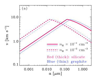
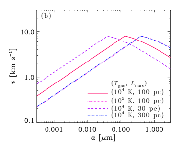
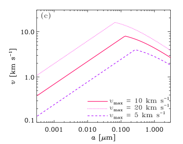
Figure 1: Grain velocity as a function of grain radius $a$. We adopt the fiducial values for the parameters but vary one of them. (a) Dependence on hydrogen number density $n_{\mathrm{H}}$. The solid and dotted lines present the cases with $n_{\mathrm{H}}=0.1$ and 0.01 cm^-3, respectively. The thick (red) and thin (blue) lines show the results for silicate and graphite, respectively (i.e. different grain material densities). (b) Dependence on gas temperature $T_{\mathrm{gas}}$ and maximum turbulence eddy size $L_{\mathrm{max}}$. The solid line shows the fiducial case. The dotted line presents the case where the temperature is varied to $10^{5}$ K (with $L_{\mathrm{max}}=100$ pc). The dashed and dot–dashed lines indicate $L_{\mathrm{max}}=30$ and 300 pc, respectively (with $T_{\mathrm{gas}}=10^{4}$ K). Note that the dotted and dot–dashed lines almost overlap. (c) Dependence on the velocity of the largest eddy, $v_{\mathrm{max}}$. The solid, dotted, and dashed lines present $v_{\mathrm{max}}=10$ (fiducial), 20, and 5 km s^-1, respectively.

The impact and frequency of grain–grain collisions are affected by the grain velocity calculated by the method in Section 2.2. Because the grain velocity is important in interpreting the evolution of grain size distribution, it is useful to present it before we show the main results.

We show the dependence of grain velocity $v$ on the parameters in Fig. 1. Recall that $v$ is a function of grain radius $a$. Overall, the grain velocity increases up to a certain grain radius and decreases at large $a$. At small $a$, grains are coupled with the turbulence, so that the grain velocity follows $v^{\mathrm{(s)}}$ (equation 5). At large $a$, grains are not fully coupled even with the largest turbulence eddies, so that the grain velocity decreases with $a$ following $v^{\mathrm{(l)}}$ in equation (6). The slopes at large and small $a$ are common for all cases.

In Fig. 1(a), we show the effect of gas density on the grain velocity. If the gas is denser, the grain velocity is reduced at small $a$ because of stronger gas drag (i.e. grains are coupled with smaller-scale motions, which have lower velocities). On the other hand, the grain velocity is raised at large $a$ in denser environments because the decoupling effect becomes weaker (i.e. the grain motion is more efficiently fluctuated by the largest-scale turbulent motions). Thus, the gas density has an opposite effect between small and large grains. In general, if the grains are more easily coupled dynamically with the gas, the velocity at small $a$ decreases and that at large $a$ increases. The peak velocity does not change as long as $v_{\mathrm{max}}$ is fixed. In the same figure, we also examine the grain material dependence. Graphite is more efficiently coupled with the turbulence than silicate because of its smaller inertia. Therefore, graphite grains have lower velocities at small $a$ and higher velocities at large $a$ than silicate. However, the difference in the grain velocities between silicate and graphite is small compared with that caused by other parameters. Thus, we use the grain velocities calculated for silicate in this paper.

In Fig. 1(b), we present the dependence on $T_{\mathrm{gas}}$ and $L_{\mathrm{max}}$. If $T_{\mathrm{gas}}$ is higher, the grain–gas coupling becomes more efficient because of a higher collision rate between gas and dust; thus, the grain velocities are lower at small $a$ and higher at large $a$. On the other hand, if $L_{\mathrm{max}}$ is larger, the turbulent velocity is reduced (equation 1). Accordingly, the grain motion responds to the turbulent motion more easily, which means that the grains are more efficiently coupled with the turbulence. Thus, for larger $L_{\mathrm{max}}$, the grain velocities become lower at small $a$ and higher at large $a$. Note that the same value of $T_{\mathrm{gas}}L_{\mathrm{max}}^{2}$ produces the same result because of the scaling in equation (5).

In Fig. 1(c), we examine the dependence on $v_{\mathrm{max}}$. We observe that $v_{\mathrm{max}}$ affects the grain velocities at all grain radii in the same direction. In addition, the grain radius where the grain velocity peaks shifts towards smaller $a$ for larger $v_{\mathrm{max}}$ since grains are less coupled with higher-velocity turbulent motions (owing to shorter turn-over time-scales). It is important to note that only $v_{\mathrm{max}}$ changes the overall grain velocity level (or the peak grain velocity), while the other parameters investigated above only vary the grain radius at which the grain velocity peaks.

3.2 Evolution of grain size distribution

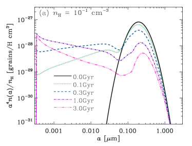
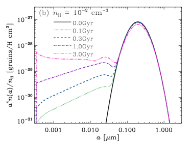
Figure 2: Evolution of grain size distribution by shattering. The solid, dotted, dashed, dot–dashed, and triple-dot–dashed lines show the results at $t=0$ (initial condition), 0.1, 0.3, 1, and 3 Gyr, respectively. We show the results for (a) $n_{\mathrm{H}}=10^{-1}$ cm^-3 and (b) $n_{\mathrm{H}}=10^{-2}$ cm^-3 with the other parameters fixed to the fiducial values (Table 1). Note that the vertical axis $a^{4}n(a)/n_{\mathrm{H}}$ is proportional to the mass-weighted grain size distribution per $\log a$ relative to the gas mass. In this expression, the peak of the initial condition is located at $a=a_{0}\exp(3\sigma^{2})\simeq 0.19~{}\micron$.

Based on the above results for the grain velocities, we examine the evolution of grain size distribution focusing on the dependences on the following parameters: $n_{\mathrm{H}}$, $L_{\mathrm{max}}$, and $v_{\mathrm{max}}$. The gas temperature and the maximum turbulence eddy size are degenerate in such a way that the same value of $T_{\mathrm{gas}}L_{\mathrm{max}}^{2}$ predicts the same evolution of grain size distribution as mentioned above. In other words, the case of $T_{\mathrm{gas}}=10^{5}$ K (with $L_{\mathrm{max}}=100$ pc) can be effectively examined by $L_{\mathrm{max}}\sim 30$ pc (with $T_{\mathrm{gas}}=10^{4}$ K). Since $v_{\mathrm{max}}$ and $n_{\mathrm{H}}$ affect the grain–grain collision rate directly, we examine the dependence on these quantities separately. We move one parameter and fix the others to the fiducial values (Table 1).

We show the evolution of grain size distribution in Fig. 2 for $n_{\mathrm{H}}=10^{-1}$ and $10^{-2}$ cm^-3. For $n_{\mathrm{H}}=10^{-1}$ cm^-3, we observe that an appreciable fraction of large grains are shattered on a time-scale of a few $\times 10^{8}$ yr. In contrast, in the case of $n_{\mathrm{H}}=10^{-2}$ cm^-3, the abundance of small grains is much lower than that of large grains even at $t=3$ Gyr. The gas density affects the grain size distribution in the following two ways: one is that the grain–grain collision rate is proportional to $n_{\mathrm{H}}$ (under a fixed dust-to-gas ratio), and the other is that the grain velocity decreases at $a\sim 0.1~{}\micron$ for lower $n_{\mathrm{H}}$ because the grains are less coupled with the largest eddies (Fig. 1a). Because of the second effect, the shattering time-scale becomes further longer than expected from a simple scaling $\propto n_{\mathrm{H}}^{-1}$ for lower densities. Thus, the small-grain production rate by shattering is very sensitive to the gas density.

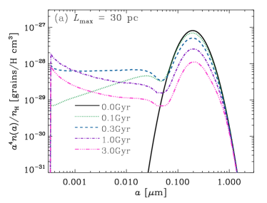
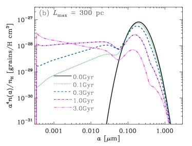
Figure 3: Same as Fig. 2(a) but for $L_{\mathrm{max}}=30$ and 300 pc in Panels (a) and (b), respectively. For the other quantities, we adopt the fiducial values (Table 1). Note that the case with $L_{\mathrm{max}}=100$ pc is shown in Fig. 2(a).

Next, we examine the effect of $L_{\mathrm{max}}$ in Fig. 3. At $t=0.3$ and 1 Gyr, small-grain production for $L_{\mathrm{max}}=30$ and 300 pc is slightly less efficient compared with the results for $L_{\mathrm{max}}=100$ pc (note that the case with $L_{\mathrm{max}}=100$ pc is shown in Fig. 2a). This is because the grain radius at which the grain velocity peaks is a little off the peak of grain size distribution (Fig. 1b). In other words, $L_{\mathrm{max}}=100$ pc is optimum for shattering if the characteristic grain radius is $a_{0}\simeq 0.1~{}\micron$. This means that the energy input to turbulence on a spatial scale of $\sim 100$ pc is favoured for small-grain production. Note again that the same result is obtained for the same value of $T_{\mathrm{gas}}L_{\mathrm{max}}^{2}$. Thus, we can also conclude that $T_{\mathrm{gas}}=10^{4}$ K is favoured for small-grain production as long as $a_{0}\simeq 0.1~{}\micron$.

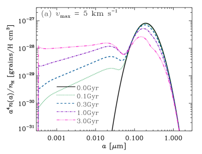
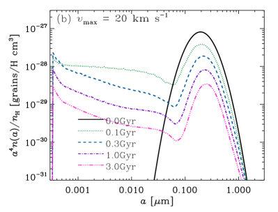
Figure 4: Same as Fig. 2(a) but for $v_{\mathrm{max}}=5$ and 20 km s^-1 in Panels (a) and (b), respectively. For the other quantities, we adopt the fiducial values. Note that the case with $v_{\mathrm{max}}=10$ km s^-1 is shown in Fig. 2(a).

Finally, we examine the effect of $v_{\mathrm{max}}$. In Fig. 4, we show the results for $v_{\mathrm{max}}=5$ and 20 km s^-1. As expected, small $v_{\mathrm{max}}$ predicts inefficient shattering because of reduced grain–grain collision rates and small impact energies. For $v_{\mathrm{max}}$ as large as 20 km s^-1, shattering disrupts not only large grains but also small grains, because the grain velocity peaks at $a<0.1~{}\micron$ and it is as high as $\sim$10 km s^-1 in a wide range of grain radii. Therefore, the overall grain abundance also decreases (recall that we remove grains shattered into $a<3$ Å). This also means that shattering does not act as a production mechanism of small $\sim 0.01~{}\micron$) grains, which affect the UV reddening, if the turbulence velocity is too high.

3.3 Evolution of extinction

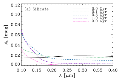
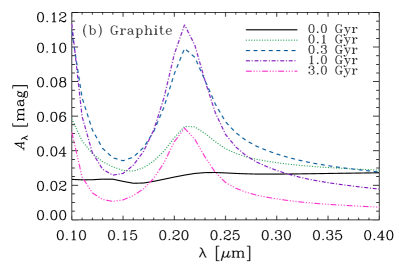
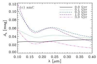
Figure 5: Wavelength dependence of extinction ($A_{\lambda}$) for (a) silicate, (b) graphite, and (c) amC. The solid, dotted, dashed, dot–dashed, and triple-dot–dashed lines show the results at $t=0$ (initial), 0.1, 0.3, 1, and 3 Gyr, respectively. We adopt $N_{\mathrm{H}}=10^{19.5}$ cm^-3, but the resulting extinction is simply proportional to $N_{\mathrm{H}}$.

Before examining the reddening curves, we show the evolution of extinction, $A_{\lambda}$, with the fiducial parameter values. In Fig. 5, we show the time variation of $A_{\lambda}$ (the extinction as a function of rest-frame wavelength) for silicate, graphite, and amC. We observe that the initial extinction has a flat dependence on the the wavelength for all the grain species. Thus, there is no significant reddening in the initial condition, which confirms that the grain size distribution dominated by large grains cannot explain the reddening observed for Mg ii absorbers. As small grains are produced by shattering, the extinction rises steeply at short wavelengths up to $t\sim 0.3$–1 Gyr. After that, the extinction decreases at almost all wavelengths because the loss from the lower grain radius boundary becomes significant. This grain loss is negligible up to $t=0.3$ Gyr, and the mass fraction of lost grains becomes 25 per cent at $t=1$ Gyr and 66 per cent at $t=3$ Gyr in the fiducial case. Thus, the extinction at short wavelengths is the most enhanced at $t\sim 0.3$–1 Gyr, which can be regarded as a time-scale of extinction curve steepening.

The wavelength dependence of $A_{\lambda}$ is sensitive to the grain species. Graphite has a prominent bump at 2175 Å. This could help explaining the reddening from optical wavelengths to $\lambda\sim 0.2~{}\micron$. Both silicate and amC have rising reddening towards shorter wavelengths except for the small bump of amC around $\lambda\sim 0.25~{}\micron$. Thus, silicate and/or amC could be responsible for rising extinction towards far-UV wavelengths.

The evolution of extinction shown here for the fiducial case gives a basis on which we interpret the evolution of reddening curve. With $n_{\mathrm{H}}=10^{-1}$ cm^-3, the variation of the other parameters broadly changes the time-scale of steepening the UV extinction but the maximum steepness of the extinction curve does not exceed the above fiducial case significantly. For $n_{\mathrm{H}}=10^{-2}$ cm^-3, the wavelength dependence of $A_{\lambda}$ remains flat because of inefficient shattering. We mention the parameter dependence again when we discuss the reddening in Section 3.4.

3.4 Reddening curves

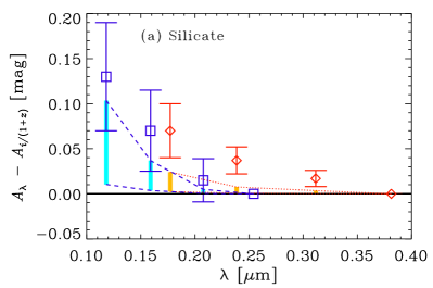
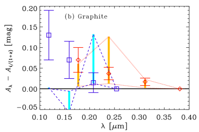
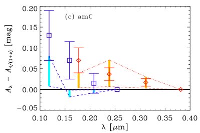
Figure 6: Reddening curves (i.e. extinction relative to the $i$-band extinction) for (a) silicate, (b) graphite, and (c) amC in the rest frame at $z=1$ and 2. We adopt the grain size distribution for the fiducial case at $t=3\times 10^{8}$ yr. The orange and light blue bars (connected by the lines in the same colour) show the theoretically predicted ranges of reddening in the SDSS $u$, $g$, and $r$ bands at $z=1$ and 2, respectively. The range of each bar corresponds to $N_{\mathrm{H}}=10^{19}$–$10^{20}$ cm^-2. The red diamonds and blue squares with error bars show the observational data of Mg ii absorbers at $z=1$ and 2, respectively, taken from MF12, with the errors expanded by a factor of 3 for a conservative comparison.

Based on the grain size distributions shown above, we calculate the reddening curves by the method explained in Section 2.4. Recall that the reddening curve is the difference between the extinction at rest-frame wavelength $\lambda$ and that in the $i$-band in the observer’s frame [rest-frame wavelengths $i/(1+z)=0.38$ and 0.25 $\micron$ at $z=1$ and 2, respectively]; that is, $A_{\lambda}-A_{i/(1+z)}$ as a function of $\lambda$. Recall that we adopt the observational data taken from MF12. For a conservative comparison, the errors in MF12 are expanded by a factor of 3. We use the grain size distribution at $t=0.3$ Gyr. After $t=1$ Gyr, the grain abundance starts to decrease, so that the reddening is simply reduced by the effect of grain mass loss. Moreover, the probable lifetime of the IGM clumps is $\lesssim\mbox{a few}\times 10^{8}$ yr (Introduction). At $t\lesssim 0.1$ Gyr, the grain size distribution does not develop enough to steepen the reddening curve. Thus, we here judge if the steepening of reddening curve occurs or not by showing the results at $t=0.3$ Gyr. Considering the uncertainties in $N_{\mathrm{H}}$, we show the range of reddening expected for $N_{\mathrm{H}}=10^{19}$–$10^{20}$ cm^-2 following HL20.

In Fig. 6, we present the reddening curves corresponding to the grain size distributions shown in Fig. 2 (the fiducial case) at $t=0.3$ Gyr for silicate, graphite, and amC. To avoid overlaying reddening curves at two redshifts, we show the reddening values only at the wavelengths where observational data are available, presenting the range of the reddening corresponding to $N_{\mathrm{H}}=10^{19}$–$10^{20}$ cm^-2. Naturally, the continuous shape of reddening curve for $\lambda$ preserves that of extinction curve shown in Fig. 5. As we observe in Fig. 6, significant reddening emerges, but the details depend on the grain species. For silicate, the predicted reddening is almost comparable to the observational data at $z=2$, but is significantly smaller than the observations at $z=1$. The difference in the calculated reddening curves between $z=1$ and 2 is simply due to the different reference wavelengths [$i/(1+z)$], since we use the same grain size distribution for both redshifts. Graphite, in contrast, reproduces the data points at $z=1$ better than at $z=2$. The enhancement at $\lambda\sim 0.20$–0.25 $\micron$ is due to the 2175 Å bump caused by small graphite grains. The other carbonaceous material, amC, reproduces the data at $z=1$ except for the shortest wavelength, but not those at $z=2$. Note that the reddening can be negative because $A_{\lambda}$ is not a monotonic function of $\lambda$, especially for the reddening curve at $z=2$, whose zero-point is set near the 2175 Å bump of graphite and the small 0.25 $\micron$ bump of amC.

Overall, compared with the initial extremely small reddening ($\lesssim 10^{-3}$), the reddening curve is steepened by shattering. It is interesting to point out that silicate and carbonaceous dust explain the steepening in a complementary way in the sense that the former and the latter species better explain the reddening at $z=1$ and 2, respectively (see also Section 4.1). This implies that a mixture of silicate and carbonaceous dust or different dust materials at different redshifts better explain the observed reddening curves.

Now we discuss the dependence on the parameters, whose effects on the grain size distribution have already been examined in Section 3.2. As shown above, for a lower value of $n_{\mathrm{H}}=10^{-2}$ cm^-3, the efficiency of small-grain production is lower. In this case, we confirm that the reddening is $\lesssim 10^{-3}$. Thus, local density enhancement to $n_{\mathrm{H}}\sim 10^{-1}$ cm^-3 as observationally suggested by Lan & Fukugita (2017) is necessary to explain the reddening in the CGM.

In our model, the fiducial case at $t\sim 0.3$ Gyr gives the largest reddening. Other cases with varied parameters are described as follows (we only change the parameter of interest with the others fixed to the fiducial values as we did above). In the case of $L_{\mathrm{max}}=30$ pc, the reddening at $t=0.3$ Gyr is roughly half of that for the fiducial case. The reddening remains low in this case, reflecting less efficient shattering than in the fiducial case (Section 3.2). The reddening reaches to a level comparable to that of the fiducial case at $t\sim 1$ Gyr in the case of $L_{\mathrm{max}}=300$ pc, while its level is half at $t=0.3$ Gyr. Recall that the small-grain production is the most efficient around the fiducial value, $L_{\mathrm{max}}=100$ pc, since the grain velocity as a function of grain radius for $L_{\mathrm{max}}=100$ pc peaks around $a\sim 0.1~{}\micron$, coinciding with the characteristic grain radius $a_{0}$ of the initial grain size distribution. As mentioned above, the same value of $T_{\mathrm{gas}}L_{\mathrm{max}}^{2}$ produces the same grain size distribution. This means that, under a fixed $L_{\mathrm{max}}=100$ pc, the case with $T_{\mathrm{max}}=10^{4}$ K is optimum in causing reddening.

The grain size distribution also depends on $v_{\mathrm{max}}$. As shown in Fig. 1(c), the grain velocities at all radii monotonically increases as $v_{\mathrm{max}}$ increases. Thus, the reddening curve is steepened at an earlier stage for larger $v_{\mathrm{max}}$. A comparable reddening curve for $v_{\mathrm{max}}=10$ km s^-1 at $t=0.3$ Gyr is reproduced with $v_{\mathrm{max}}=20$ km s^-1 at $t=0.1$ Gyr and with $v_{\mathrm{max}}=5$ km s^-1 at $t=1$ Gyr. The reddening declines after these times because of the loss of small grains from the lower grain radius boundary. Thus, the maximum turbulence velocity determines the overall time-scale on which shattering steepens the reddening curve.

We note that the assumed values of $N_{\mathrm{H}}$ and $\mathcal{D}_{0}$ are uncertain. Since the resulting reddening is proportional to $N_{\mathrm{H}}\mathcal{D}_{0}$, a factor 2 increase in $N_{\mathrm{H}}\mathcal{D}_{0}$ would easily explain the observed level of reddening curves, although we do not fine-tune these parameters further.

The reddening is also affected by the choice of the smallest grain radius, which we assume to be 3 Å. Some authors adopted larger values for the minimum grain radius in modelling the grain size distribution (e.g. Silvia et al., 2010; Kirchschlager et al., 2019; Hoang, 2021). As argued by Nozawa & Fukugita (2013), the smallest grain radius only has a minor influence on the extinction curves. In our case, if we simply eliminate the grains with $a<10$ Å (without keeping the dust mass), the reduction of reddening at the shortest wavelength for silicate is 15 per cent, while that at the bumps of carbonaceous grains is 20 per cent.

4 Discussion

4.1 Mixture of grain species

In the above, we have shown that steepening does occur by shattering associated with cool clumps in the CGM, concluding that shattering could be a cause of the reddening observed for Mg ii absorbers. However, the degree of reddening depends on the grain species, and it seems to be difficult to explain the reddening data at both $z=1$ and 2 with a single grain species. Interestingly, silicate and carbonaceous dust are supplementary in the sense that the former species explains the reddening at $z=1$ relatively well while the latter is more favoured at $z=2$. In reality, it is more likely that the IGM dust is composed of multiple species. Thus, it is intriguing to investigate if a mixture of silicate and carbonaceous species explains the reddenings at $z=1$ and 2 at the same time.

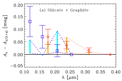
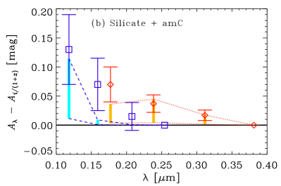
Figure 7: Same as Fig. 6 but for the mixture of silicate and carbonaceous dust with a mass ratio of 0.54:0.46. Panels (a) and (b) show the mixtures of silicate and graphite, and of silicate and amC, respectively.

Here we investigate the mixture of silicate and graphite as an example of multiple-species mixture. We assume the mass ratio of silicate to graphite to be 0.54:0.46 (Hirashita & Aoyama, 2019) and add the extinctions of the two species at $t=0.3$ Gyr with the above weight. This mass ratio is valid for the Milky Way extinction curve (Hirashita & Aoyama, 2019), and the almost half–half ratio is also useful to maximize the effect of the mixture. In Fig. 7(a), we show the results. As expected, the resulting reddening is significant at both $z=1$ and 2, although the reddening data at the shortest wavelengths are better explained by the single-species (silicate) case. However, we emphasize that the mixture makes the behaviour of reddening along the wavelength axis more moderate in the sense that the specific feature of a certain single species becomes less prominent. We note that graphite-dominated dust is not favoured by the extinction curve derived for QSO absorbers by York et al. (2006), which does not show any significant 2175 Å bump.

We also examine the mixture of silicate and amC in Fig. 7(b), where we adopt the same silicate-to-carbonaceous dust mass ratio as above. We confirm that the mixture produces significant reddening at both $z=1$ and 2. Which of graphite and amC better explains the reddening data depends on the wavelength; thus, we are not able to conclude which dust species is favourable.

We also point out that the ratio between silicate and carbonaceous dust could depend on the redshift. Since clarifying the redshift dependence theoretically is beyond the scope of our formulation, we leave the evolution of grain species in the CGM for a future work.

4.2 Possible solutions to the underproducing tendencies

In the above results, both silicate and carbonaceous species tend to underproduce the observed reddening curves, especially at short wavelengths. As mentioned above, the extinction is proportional to the product of $N_{\mathrm{H}}$ and $\mathcal{D}$, both of which are uncertain. We already assumed $\mathcal{D}_{0}=0.006$ (the initial value of $\mathcal{D}$), which is appropriate in solar metallicity environments. If Mg ii absorbers trace metal-enriched gas originating from the central galaxy, it is possible that the dust-to-gas ratio is higher. If the dust-to-gas ratio is, for example, twice higher than assumed in this paper, the reddening curves are almost consistent with the observational data. Adopting a fixed range of $N_{\mathrm{H}}$ might be too simplistic; indeed, there is probably a larger dispersion in $N_{\mathrm{H}}$ for Mg ii absorbers with an indication of redshift evolution (Lan & Fukugita, 2017). Thus, more sophisticate modelling may be necessary; for example, the detailed distribution function of $N_{\mathrm{H}}$ dependent on $z$ would be worth modelling. However, we emphasize that, even with our simple models, shattering produces significant reddening, which is consistent with the observational data within a factor of $\sim$2.

Lan & Fukugita (2017) showed that the column density of Mg ii absorbers becomes higher with redshift as $N_{\mathrm{H}}\propto(1+z)^{1.9}$. Thus, we expect that $N_{\mathrm{H}}$ is $(3/2)^{1.9}\simeq 2.2$ times higher at $z=2$ than at $z=1$. This could make it easier to explain the data points at $z\sim 2$. We should keep in mind, however, that $\mathcal{D}$ may also be different between $z=1$ and 2 (Péroux & Howk, 2020).

The treatment of shattered fragments could be uncertain, especially for extremely small grains. Applying the bulk material properties to grains near the lower grain radius boundary ($a\sim 3$ Å) may not be valid. For example, if such small grains are not efficiently disrupted by shattering, the grains are not lost by shattering as efficiently as we calculated in this paper. However, it is difficult to introduce this kind of effect since we do not have knowledge on the disruptive properties at such small grain radii. Although it is difficult to fully address this issue, we make an attempt of effectively examining the effect of grain mass loss in shattering in the following.

In the above, the dust abundance (dust-to-gas ratio $\mathcal{D}$) decreases as a function of time, and the decreasing effect is prominent at $t\gtrsim 1$ Gyr in the fiducial case. To mimic the case where small grains are not efficiently shattered, we adopt $\mathcal{D}=0.006$ (the initial value) instead of the value at each age, in calculating the extinction (equation 12). This effectively cancels out the effect of grain mass loss by artificially adjusting $\mathcal{D}$. This ‘correction’ for the dust mass loss is important only at $t\gtrsim 1$ Gyr. Thus, we only show in Fig. 8 the result at $t=1$ Gyr for the same mixed cases as in Fig. 7 (at $t=3$ Gyr, the correction factor is too large to make a meaningful prediction). Comparing Fig. 8 with Fig. 7, we find that the reddening is enhanced. Similar enhancement is also expected for reddening curves of single species. Thus, a longer shattering duration without grain mass loss may be a solution for the underprediction of reddening.

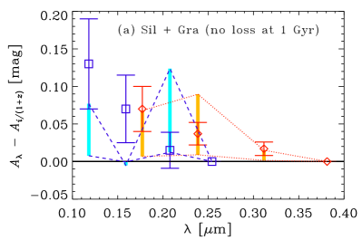
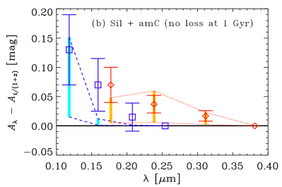
Figure 8: Same as Fig. 7 but with the correction for dust mass loss using the renormalization described in the text (to supplement the lost dust).

4.3 Prospects for further modelling

In this paper, we have focused on shattering in the CGM. Here we discuss our results in the context of overall dust evolution in the CGM.

Aoyama et al. (2018), using a cosmological simulation, showed that the dust-to-metal ratio decreases with the distance from the galaxy centre in the CGM. This is due to sputtering in the hot gas. However, in their simulation, the formation of cool clumps in the CGM cannot be spatially resolved. The density structures in the CGM calculated by cosmological simulations still depend on the spatial resolution (e.g. van de Voort et al., 2019), and it is in general extremely difficult for cosmological simulations to resolve a scale of a few tens of parsecs unless we develop some dedicated high-resolution scheme (Hummels et al., 2019). Thus, it is necessary to somehow include shattering associated with cool clumps by developing a sub-grid model. The formulation or the result of this paper could be used as a sub-grid input model in cosmological simulations.

There are some possible effects of shattering in the CGM. First, since the grains become smaller, they are more efficiently destroyed by sputtering once they are injected into the hot ($T_{\mathrm{gas}}\gtrsim 10^{6}$ K) gas. Thus, the modification of grain size distribution by shattering could alter the grain destruction rate by sputtering in the CGM. Secondly, we expect that the grain size distribution is inhomogeneous in the CGM with more small grains in cool clumps. Thus, if the dust observation is biased to the cool medium (such as Mg ii absorbers), it selectively see regions where UV reddening curves are steepened. Thirdly, the photoelectric heating rate of the CGM and IGM depends on the grain radius. Small grains tend to be more efficient in photoelectric heating with a fixed dust mass abundance (Inoue & Kamaya, 2003, 2004). Thus, the small-grain production by shattering is important for the heating rate in the CGM (and in the IGM if the grains are transported to a wide area in the Universe). It is interesting to examine these effects of small-grain production self-consistently by including shattering in the CGM in cosmological simulations, or to develop some analytical model that could include all relevant processes for the enrichment and processing of dust in the CGM.

5 Conclusion

We investigate the small-grain production in the CGM through shattering, which could occur efficiently in turbulent media with a high enough gas density. Cool ($T_{\mathrm{gas}}\sim 10^{4}$ K) clumps traced by Mg ii absorbers are possible sites that have favourable conditions for shattering. We calculate the evolution of grain size distribution by shattering in turbulent cool gas and examine if small grains are efficiently produced on a reasonable time-scale (i.e. within the typical lifetime of the cool gas $\sim\mbox{a few}\times 10^{8}$ yr).

We solve the shattering equation in a condition relevant for cool clumps in the CGM. For the initial condition, we adopt a lognormal grain size distribution with characteristic grain radius $a_{0}\sim 0.1~{}\micron$. This is because previous studies suggested that grains transported from the central galaxy to the CGM are dominated by such large grains. This initial condition also serves to examine if shattering could produce a sufficient number of small grains within a reasonable time even from the large-grain-dominated grain size distribution. The grain motion is assumed to be induced by turbulence whose maximum size is determined roughly by the clump size ($L_{\mathrm{max}}\sim 100$ pc). It is also expected that the maximum velocity of turbulent motion is of the order of $v_{\mathrm{max}}\sim 10$ km s^-1, which is comparable to the sound speed of the cool gas. The initial dust-to-gas ratio is fixed to $\mathcal{D}_{0}=0.006$ as derived from observations (noting that the time-scale simply scales as $\mathcal{D}_{0}^{-1}$).

We find that small-grain production efficiently occurs in the fiducial parameter set ($n_{\mathrm{H}}=0.1$ cm^-3, $T_{\mathrm{gas}}=10^{4}$ K, $L_{\mathrm{max}}=100$ pc, and $v_{\mathrm{max}}=10$ km s^-1) on a time-scale of a few $\times 10^{8}$ yr, comparable to the lifetime of cool clumps. It also turns out that the above values for $n_{\mathrm{H}}$, $T_{\mathrm{gas}}$ and $L_{\mathrm{max}}$ are optimum for small-grain production in the sense that the peak of the grain velocity as a function of grain radius is located around the characteristic grain radius $a_{0}\sim 0.1~{}\micron$. Note that the above fiducial values are chosen not for optimizing the shattering efficiency but based on the values suggested from observations of Mg ii absorbers.

We further calculate reddening curves based on the above grain size distributions but using various dust species. We find that the reddening becomes significant at $t\sim\mbox{a few}\times 10^{8}$ yr in the fiducial parameter values. The time-scale of reddening is similar to the lifetime of cool clumps in the CGM. Therefore, we conclude that shattering in the CGM is a probable reason for the observed reddening. The reddening curves are sensitive to the grain species. Silicate explains the reddening observed at $z=2$ while it underpredicts that at $z=1$. In contrast, graphite and amC explain the reddening observed at $z=1$ more easily than that at $z=2$. The difference between $z=1$ and 2 is due to the different rest-frame wavelengths, $i/(1+z)$, used for the zero point (note that our model applies the same grain size distribution to both redshifts). A mixture (or redshift-dependent fraction) of silicate and carbonaceous dust is favoured to explain the reddenings at $z=1$ and 2 simultaneously.

There is still a tendency that our model underpredicts the reddening. Considering that the predicted reddening level is proportional to the hydrogen column density and the dust-to-gas ratio, the underprediction could be associated with the large uncertainties in these quantities. Moreover, the treatment of shattering at very small grain radii ($a\lesssim 0.001~{}\micron$) may need improvement since we simply apply bulk material properties. If such extremely small grains are not efficiently shattered, they remain to contribute to the reddening.

Since shattering associated with cool clumps has proven to be important, it is desirable to somehow include this process in dust evolution models in a cosmological volume. For example, a sub-grid model could be developed for shattering to be included in a cosmological hydrodynamic simulation. This kind of development will be worth tackling in a future work.

Data Availability

Data related to this publication and its figures are available on request from the corresponding author.

References

- Aoyama et al. (2018) Aoyama S., Hou K.-C., Hirashita H., Nagamine K., Shimizu I., 2018, MNRAS, 478, 4905
- Armillotta et al. (2017) Armillotta L., Fraternali F., Werk J. K., Prochaska J. X., Marinacci F., 2017, MNRAS, 470, 114
- Asano et al. (2013) Asano R. S., Takeuchi T. T., Hirashita H., Nozawa T., 2013, MNRAS, 432, 637
- Bekki et al. (2015) Bekki K., Hirashita H., Tsujimoto T., 2015, ApJ, 810, 39
- Ben Bekhti et al. (2009) Ben Bekhti N., Richter P., Winkel B., Kenn F., Westmeier T., 2009, A&A, 503, 483
- Bianchi & Ferrara (2005) Bianchi S., Ferrara A., 2005, MNRAS, 358, 379
- Bohren & Huffman (1983) Bohren C. F., Huffman D. R., 1983, Absorption and Scattering of Light by Small Particles. Wiley, New York
- Buie et al. (2018) Buie E., Gray W. J., Scannapieco E., 2018, ApJ, 864, 114
- Buie et al. (2020) Buie E., Gray W. J., Scannapieco E., Safarzadeh M., 2020, ApJ, 896, 136
- Chen et al. (2010) Chen H.-W., Helsby J. E., Gauthier J.-R., Shectman S. A., Thompson I. B., Tinker J. L., 2010, ApJ, 714, 1521
- Davies et al. (1998) Davies J. I., Alton P., Bianchi S., Trewhella M., 1998, MNRAS, 300, 1006
- Dwek (1987) Dwek E., 1987, ApJ, 322, 812
- Ferrara et al. (1991) Ferrara A., Ferrini F., Barsella B., Franco J., 1991, ApJ, 381, 137
- Fielding et al. (2020) Fielding D. B., Ostriker E. C., Bryan G. L., Jermyn A. S., 2020, ApJ, 894, L24
- Fukugita (2011) Fukugita M., 2011, preprint (arXiv:1103.4191)
- Guillet et al. (2011) Guillet V., Pineau Des Forêts G., Jones A. P., 2011, A&A, 527, A123
- Hirashita & Aoyama (2019) Hirashita H., Aoyama S., 2019, MNRAS, 482, 2555
- Hirashita & Inoue (2019) Hirashita H., Inoue A. K., 2019, MNRAS, 487, 961
- Hirashita & Kobayashi (2013) Hirashita H., Kobayashi H., 2013, Earth, Planets, and Space, 65, 1083
- Hirashita & Li (2013) Hirashita H., Li Z.-Y., 2013, MNRAS, 434, L70
- Hirashita & Lin (2020) Hirashita H., Lin C.-Y., 2020, Planet. Space Sci., 183, 104504
- Hirashita & Yan (2009) Hirashita H., Yan H., 2009, MNRAS, 394, 1061
- Hirashita et al. (2021) Hirashita H., Il’in V. B., Pagani L., Lefèvre C., 2021, MNRAS, 502, 15
- Hoang (2021) Hoang T., 2021, ApJ, 907, 37
- Hou et al. (2016) Hou K.-C., Hirashita H., Michałowski M. J., 2016, PASJ, 68, 94
- Hou et al. (2017) Hou K.-C., Hirashita H., Nagamine K., Aoyama S., Shimizu I., 2017, MNRAS, 469, 870
- Hummels et al. (2019) Hummels C. B., et al., 2019, ApJ, 882, 156
- Inoue & Kamaya (2003) Inoue A. K., Kamaya H., 2003, MNRAS, 341, L7
- Inoue & Kamaya (2004) Inoue A. K., Kamaya H., 2004, MNRAS, 350, 729
- Jones et al. (1994) Jones A. P., Tielens A. G. G. M., Hollenbach D. J., McKee C. F., 1994, ApJ, 433, 797
- Jones et al. (1996) Jones A. P., Tielens A. G. G. M., Hollenbach D. J., 1996, ApJ, 469, 740
- Kirchschlager et al. (2019) Kirchschlager F., Schmidt F. D., Barlow M. J., Fogerty E. L., Bevan A., Priestley F. D., 2019, MNRAS, 489, 4465
- Kobayashi & Tanaka (2010) Kobayashi H., Tanaka H., 2010, Icarus, 206, 735
- Kusaka et al. (1970) Kusaka T., Nakano T., Hayashi C., 1970, Progress of Theoretical Physics, 44, 1580
- Lan (2020) Lan T.-W., 2020, ApJ, 897, 97
- Lan & Fukugita (2017) Lan T.-W., Fukugita M., 2017, ApJ, 850, 156
- Lan & Mo (2019) Lan T.-W., Mo H., 2019, MNRAS, 486, 608
- Li et al. (2020) Li Z., Hopkins P. F., Squire J., Hummels C., 2020, MNRAS, 492, 1841
- Liang & Remming (2020) Liang C. J., Remming I., 2020, MNRAS, 491, 5056
- Masaki & Yoshida (2012) Masaki S., Yoshida N., 2012, MNRAS, 423, L117
- Mattsson (2020) Mattsson L., 2020, MNRAS, 491, 4334
- McKinnon et al. (2016) McKinnon R., Torrey P., Vogelsberger M., 2016, MNRAS, 457, 3775
- Ménard & Chelouche (2009) Ménard B., Chelouche D., 2009, MNRAS, 393, 808
- Ménard & Fukugita (2012) Ménard B., Fukugita M., 2012, ApJ, 754, 116
- Ménard et al. (2010) Ménard B., Scranton R., Fukugita M., Richards G., 2010, MNRAS, 405, 1025
- Nielsen et al. (2013) Nielsen N. M., Churchill C. W., Kacprzak G. G., 2013, ApJ, 776, 115
- Nozawa & Fukugita (2013) Nozawa T., Fukugita M., 2013, ApJ, 770, 27
- Ormel & Cuzzi (2007) Ormel C. W., Cuzzi J. N., 2007, A&A, 466, 413
- Ormel et al. (2009) Ormel C. W., Paszun D., Dominik C., Tielens A. G. G. M., 2009, A&A, 502, 845
- Peek et al. (2015) Peek J. E. G., Ménard B., Corrales L., 2015, ApJ, 813, 7
- Pei (1992) Pei Y. C., 1992, ApJ, 395, 130
- Péroux & Howk (2020) Péroux C., Howk J. C., 2020, ARA&A, 58, 363
- Prochaska & Hennawi (2009) Prochaska J. X., Hennawi J. F., 2009, ApJ, 690, 1558
- Rauch et al. (1999) Rauch M., Sargent W. L. W., Barlow T. A., 1999, ApJ, 515, 500
- Shustov & Vibe (1995) Shustov B. M., Vibe D. Z., 1995, Astronomy Reports, 39, 578
- Silvia et al. (2010) Silvia D. W., Smith B. D., Shull J. M., 2010, ApJ, 715, 1575
- Sparre et al. (2020) Sparre M., Pfrommer C., Ehlert K., 2020, MNRAS, 499, 4261
- Steidel et al. (1994) Steidel C. C., Dickinson M., Persson S. E., 1994, ApJ, 437, L75
- Thompson et al. (2016) Thompson T. A., Quataert E., Zhang D., Weinberg D. H., 2016, MNRAS, 455, 1830
- Tielens et al. (1994) Tielens A. G. G. M., McKee C. F., Seab C. G., Hollenbach D. J., 1994, ApJ, 431, 321
- van de Voort et al. (2019) van de Voort F., Springel V., Mandelker N., van den Bosch F. C., Pakmor R., 2019, MNRAS, 482, L85
- Veilleux et al. (2005) Veilleux S., Cecil G., Bland-Hawthorn J., 2005, ARA&A, 43, 769
- Voelk et al. (1980) Voelk H. J., Jones F. C., Morfill G. E., Roeser S., 1980, A&A, 85, 316
- Weidenschilling (1977) Weidenschilling S. J., 1977, MNRAS, 180, 57
- Weingartner & Draine (2001) Weingartner J. C., Draine B. T., 2001, ApJ, 548, 296
- Werk et al. (2013) Werk J. K., Prochaska J. X., Thom C., Tumlinson J., Tripp T. M., O’Meara J. M., Peeples M. S., 2013, ApJS, 204, 17
- Werk et al. (2014) Werk J. K., et al., 2014, ApJ, 792, 8
- York et al. (2000) York D. G., et al., 2000, AJ, 120, 1579
- York et al. (2006) York D. G., et al., 2006, MNRAS, 367, 945
- Zu et al. (2011) Zu Y., Weinberg D. H., Davé R., Fardal M., Katz N., Kereš D., Oppenheimer B. D., 2011, MNRAS, 412, 1059
- Zubko et al. (1996) Zubko V. G., Mennella V., Colangeli L., Bussoletti E., 1996, MNRAS, 282, 1321
- Zubko et al. (2004) Zubko V., Dwek E., Arendt R. G., 2004, ApJS, 152, 211