:
AABI 20203rd Symposium on Advances in Approximate Bayesian Inference, 2020

Empirical Evaluation of Biased Methods for Alpha Divergence Minimization

1 Introduction

Traditional variational inference (VI) minimizes the “exclusive” KL divergence $\mathrm{KL}(q\|p)$ between the approximating distribution $q$ and the target $p$. There has been great recent interest in methods to minimize other alpha-divergences, such as the “inclusive” KL divergence, $\mathrm{KL}(p\|q)$. Some methods employ unbiased gradient estimators (Dieng et al., 2017; Kuleshov and Ermon, 2017). These estimators often suffer from a high variance, difficulting optimization (Geffner and Domke, 2020). Another class of methods estimate a gradient using self-normalized importance sampling (Bornschein and Bengio, 2014; Finke and Thiery, 2019; Li and Turner, 2016). While these estimators may control variance, they do so at the cost of some bias. While some positive results have been observed for biased methods (e.g. higher log-likelihoods (Li and Turner, 2016; Dieng et al., 2017)), the magnitude of the bias and the effect it has on the distributions they return are not well understood.

In this paper we empirically evaluate biased methods for alpha-divergence minimization. In particular, we focus on how the bias affects the solutions found, and how this depends on the dimensionality of the problem. Our two main takeaways are (i) solutions returned by these methods appear to be strongly biased towards minimizers of the traditional “exclusive” KL-divergence, $\mathrm{KL}(q\|p)$. And (ii) in high dimensions, an impractically large amount of computation is needed to mitigate this bias and obtain solutions that actually minimize the alpha-divergence of interest.

Finally, we relate these results to the curse of dimensionality. In high dimensions, it is well known that self-normalized importance sampling often suffers from “weight degeneracy” (unless the number of samples used is exponential in the dimensionality of the problem (Bugallo et al., 2017; Bengtsson et al., 2008)), resulting in estimates with high bias. We empirically show that weight degeneracy does indeed occur with these estimators in cases where they return highly biased solutions.

1.1 Estimators considered

Notation: $q_{\phi}$ denotes the variational distribution parameterized by $\phi$. $z_{\phi,k}$ denotes a sample from $q_{\phi}$ obtained via reparameterization (Kingma and Welling, 2013; Titsias and Lázaro-Gredilla, 2014). $\psi$ denotes the parameters $\phi$ “protected under differentiation” (i.e. $\psi=\texttt{stop\_gradient}(\phi)$).

• For the Renyi alpha-divergence, $\mathrm{R}_{\alpha}(q||p)$, Li and Turner (2016) proposed the estimator

  $$g_{R_{\alpha}}=-\sum_{k=1}^{K}\frac{w_{\alpha,k}}{\sum_{j=1}^{K}w_{\alpha,j}}\,\nabla_{\phi}\log\frac{p(x,z_{\phi,k})}{q_{\phi}(z_{\phi,k})},\qquad\mbox{where}\qquad w_{\alpha,k}=\left(\frac{p(x,z_{\phi,k})}{q_{\phi}(z_{\phi,k})}\right)^{1-\alpha}.$$

  This is defined for $\alpha>0$. We use $\alpha=0.5$ in our experiments.

• For the “inclusive” divergence $\mathrm{KL}(p||q)$, the reweighted wake-sleep estimator (Bornschein and Bengio, 2014) (also used in Edward (Tran et al., 2016)) is given by

  $$g_{\mathrm{rws}}=\sum_{k=1}^{K}\frac{w_{k}}{\sum_{j=1}^{K}w_{j}}\,\nabla_{\phi}\log q_{\phi}(z_{\psi,k}),\qquad\mbox{where}\qquad w_{k}=\frac{p(x,z_{\phi,k})}{q_{\phi}(z_{\phi,k})}.$$

  For the same divergence, the “sticking the landing” estimator (Roeder et al., 2017) is given by

  $$g_{\mathrm{stl}}=-\sum_{k=1}^{K}\frac{w_{k}}{\sum_{j=1}^{K}w_{j}}\,\nabla_{\phi}\log\frac{p(x,z_{\phi,k})}{q_{\psi}(z_{\phi,k})},\qquad\mbox{where}\qquad w_{k}=\frac{p(x,z_{\phi,k})}{q_{\phi}(z_{\phi,k})}.$$

• For the chi divergence, $\chi^{2}(p||q)$, the CHIVI algorithm (Dieng et al., 2017) uses the estimator

  $$g_{\mathrm{chivi}}=-\sum_{k=1}^{K}\left(\frac{w_{k}}{\max_{j}w_{j}}\right)^{2}\nabla_{\phi}\log\frac{p(x,z_{\phi,k})}{q_{\phi}(z_{\phi,k})},\qquad\mbox{where}\qquad w_{k}=\frac{p(x,z_{\phi,k})}{q_{\phi}(z_{\phi,k})}.$$

  (This estimator was used by Dieng et al. (2017) in their experiments, but not in their analysis.) For the same divergence, the doubly reparameterized estimator (Tucker et al., 2018; Finke and Thiery, 2019) is given by

  $$g_{\mathrm{drep}}=-\sum_{k=1}^{K}\left(\frac{w_{k}}{\sum_{j=1}^{K}w_{j}}\right)^{2}\nabla_{\phi}\log\frac{p(x,z_{\phi,k})}{q_{\psi}(z_{\phi,k})},\qquad\mbox{where}\qquad w_{k}=\frac{p(x,z_{\phi,k})}{q_{\phi}(z_{\phi,k})}.$$

All of these estimators are asymptotically unbiased in the limit of $K\rightarrow\infty$ except for $g_{\mathrm{chivi}}$. However, the bias for finite $K$ is not well understood.

2 Empirical Evaluation

We now present an empirical evaluation of the estimators described above. We consider two scenarios for the model $p$: a simple Gaussian distribution and logistic regression. In both cases we use Adam (Kingma and Ba, 2014) with each of the gradient estimators to minimize the corresponding alpha-divergence, and compare the results obtained against the theoretically optimal ones.

2.1 Evaluation I: Gaussian Model

Model: Similarly to Neal (2011), we set the target $p$ to be a diagonal $d$-dimensional Gaussian with mean zero and variances $\sigma_{p_{i}}^{2}=0.2+9.8\frac{i}{d}$. So, the variance of the components of $p$ grows linearly from $\sigma_{p_{1}}^{2}=0.2$ to $\sigma_{p_{d}}^{2}=10$. We ran simulations for dimensionalities $d\in\{10,100,1000\}$

Variational distribution: We set $q$ to be a mean-zero isotropic Gaussian with covariance $\sigma_{q}^{2}I$. So, $q$ has a single parameter $\sigma_{q}$, which we initialize to $\sigma_{q}^{2}=9$.

Optimization details: We attempt to optimize alpha-divergences by running Adam (step-size $\eta=0.01$) for $2000$ steps using each of the gradient estimators introduced in Section 1.1. We repeat this for estimators obtained using $K$ samples, with $K\in\{10,100,1000\}$.

Baselines: In this scenario we can compute the optimal $\sigma_{q}$ to exactly minimize each of $\mathrm{KL}(q\|p)$, $\mathrm{KL}(p\|q)$, $R_{\alpha}(q\|p)$ and $\chi^{2}(p\|q)$. This gives us a clear way of visualizing the bias induced by each estimator.

Results: Fig. LABEL:fig:target_method_gauss shows how the parameter $\sigma_{q}$ evolves as optimization proceeds when using the “sticking the landing” estimator $g_{stl}$, which targets the divergence $\mathrm{KL}(p\|q)$. For low dimensions ($d=10$), the optimal value $\sigma_{q}^{*}$ is recovered almost exactly as long as $K\geq 100$ samples are used to estimate the gradients. For higher dimensions, the solution is increasingly biased towards the minimizer of $\mathrm{KL}(q||p)$. While this bias can in theory be mitigated by increasing the number of samples $K$ used to estimate the gradients, the number required becomes impractically large in high dimensions.

fig:target_method_gauss            

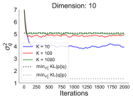
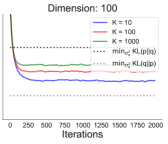
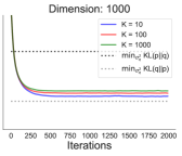
Figure 1: For high dimensions an impractically large number of samples $K$ is needed to mitigate the estimator’s bias. Optimization results when minimizing $\mathrm{KL}(p||q)$ for the synthetic Gaussian model using the biased gradient estimator $g_{stl}$ obtained using $K$ samples.

Fig. LABEL:fig:var_dim_gauss shows that a similar phenomena occurs with all other estimators introduced in Section 1.1. The plots do not show optimization traces; they show the final $\sigma_{q}^{2}$ after 2000 optimization steps as a function of the problem’s dimension. (We show raw optimization results for all estimators in Appendix A). The same conclusion as the one described above applies for all estimators (except _chivi): The methods tend to work well in low dimensions, but return suboptimal solutions that are strongly biased towards minimizers of $\mathrm{KL}(q||p)$ in higher dimensions. Again, while this bias can be mitigated by increasing the number of samples $K$ used to estimate gradients, the value of $K$ required becomes impractically large in high dimensions. (_chivi also yields suboptimal solutions in low dimensions. This is likely because this estimator uses atypical weight normalization and so is not asymptotically unbiased.)

fig:var_dim_gauss            

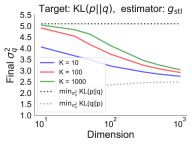
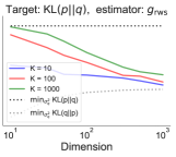
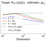
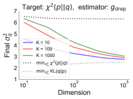
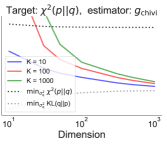
Figure 2: In high dimensions solutions are strongly biased towards minimizers of $\mathrm{KL}(q||p)$. Optimization results for all estimators for the synthetic Gaussian model, as a function of the dimensionality of the problem and the number of samples $K$ used to estimate gradients.

We believe that the suboptimality of the solutions returned by biased methods in high dimensions is related to the weight collapse effect (also known as weight degeneracy) suffered by self normalized importance sampling (Bengtsson et al., 2008). To verify this empirically, we plot the magnitude of the normalized importance weights obtained for different dimensionalities $d$ and number of samples $K$. We observe that the pairs $(d,K)$ for which solutions are highly biased correspond to the cases for which the weight collapse effect is observed (details in Appendix C and Fig. LABEL:fig:wc therein).

2.2 Evaluation II: Logistic Regression

Model: Bayesian logistic regression with two datasets: sonar ($d=61$) and a1a ($d=120$).

Variational distribution: We set $q$ to be a diagonal Gaussian, with mean $\mu_{q}$ and variance $\sigma_{q}^{2}$ (vectors of dimension $d$), with components initialized to $\mu_{q_{i}}=0$ and $\sigma_{q_{i}}^{2}=9$. (We parameterize the variance using the log-scale parameters.)

Optimization details: We attempt to optimize alpha-divergences by running Adam (step-size $\eta=0.01$) for $5000$ steps using each of the gradient estimators introduced in Section 1.1. We repeat this for estimators obtained using $K$ samples, with $K\in\{10,100,1000\}$.

Baselines: We compare against the optimal parameters $(\mu_{q}^{*},\sigma_{q}^{*})$ that minimize $\mathrm{KL}(p||q)$. While these cannot be computed in closed form, we approximate them by minimizing $\mathrm{KL}(p||q)$ using the algorithm proposed by Naesseth et al. (2020). Again, having these parameters provides a clear way of visualizing the effect of using biased gradient estimates.

Results: Fig. LABEL:fig:opt_log_reg_drep shows optimization results for the estimator $g_{\mathrm{stl}}$, which targets $\mathrm{KL}(p\|q)$. It can be observed that, for the sonar dataset ($d=61$), distributions that attain near-optimal performance are obtained using gradient estimates computed with $K\geq 100$ samples. In contrast, for the a1a dataset ($d=120$), all values of $K$ tested lead to significantly biased and suboptimal solutions. (Though, as expected, increasing the number of samples $K$ reduces the suboptimality gap.)

fig:opt_log_reg_drep      

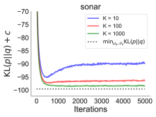
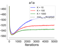
Figure 3: For the dataset with higher dimensionality the algorithm returns biased solutions that are suboptimal regardless of the number of samples $K$ used. The plots show optimization results for minimizing $\mathrm{KL}(p\|q)$ for the logistic regression model using the estimator $g_{stl}$ obtained with $K$ samples. The y-axis in the plots show the true $\mathrm{KL}(p\|q)$ (up to the additive constant $c=\log p(x)$ – which can be estimated using samples from $p(z|x)$, obtained using Stan (Carpenter et al., 2017)). The seemingly strange behavior of optimization traces is not due to bad optimization hyperparameters, but to the bias of the gradient estimator.

Fig. LABEL:fig:params_stl_logreg shows how the optimal parameters $(\mu_{q}^{*},\sigma_{q}^{*})$ compare against the parameters obtained by optimizing using the biased gradient estimator $g_{\mathrm{stl}}$. We observe two things. First, the optimal mean parameters are well-recovered for both datasets regardless of the number of samples $K$ used to estimate gradients. Second, the scale parameters recovered are biased towards minimizers of $\mathrm{KL}(q||p)$. For the sonar dataset $(d=61)$, this bias can be removed by increasing the number of samples $K$ used to estimate gradients. However, for the a1a dataset $(d=120)$, increasing $K$ to 1000 provides only a tiny improvement, suggesting a huge value for $K$ would be needed.

Results for all other estimators are similar to the ones shown in this section for _stl. We show them in Appendix B.

fig:params_stl_logreg      

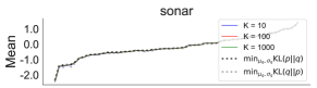
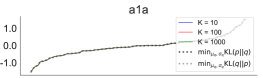
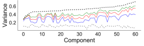
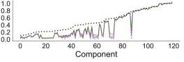
Figure 4: In high dimensions optimizing with the biased estimator leads to solutions strongly biased towards minimizers of $\mathrm{KL}(q\|p)$, and an impractically large $K$ is needed to mitigate this effect. Results for the logistic regression model with both datasets, sonar $(d=61)$ and a1a $(d=120)$. The plots show the mean and variance of each component of the variational distribution $q$ obtained by optimizing with the gradient estimator $g_{\mathrm{stl}}$ with $K$ samples. Components are sorted to facilitate visualization.

3 Conclusions

All gradient estimators analyzed are asymptotically unbiased (except $g_{\mathrm{chivi}}$). This means that, if a large enough number of samples $K$ is used to estimate gradients, these methods are guaranteed to return near-optimal solutions. In practice, however, we observe that even for very simple problems, the value of $K$ needed is typically very large.

Interestingly, solutions returned by these methods appear to be biased towards minimizers of $\mathrm{KL}(q||p)$. Upon close examination, it is not obvious why this should be true and to the best of our knowledge no theoretical support for this behavior is known. We find this surprising and consider it to be an appealing property of these methods: Even when they fail to minimize the target alpha-divergence, they do something “reasonable”, i.e. minimize the traditional divergence $\mathrm{KL}(q||p)$.

Appendix A Optimization results for all estimators with Gaussian model

fig:target_method_gauss_end            

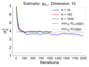
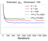
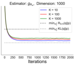
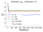
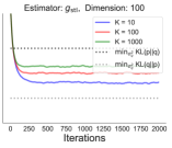
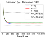
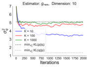
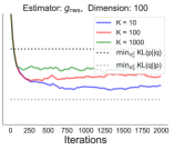
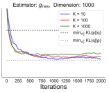
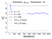
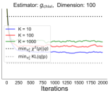
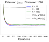
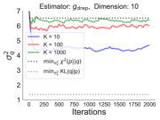
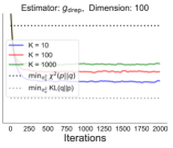
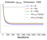
Figure 5: Optimization results for all estimators.

Appendix B Optimization results for all estimators with logistic regression model

This section shows the results obtained for the logistic regression model using all of the estimators introduced in Section 1.1. Fig. LABEL:fig:end_opt_sonar shows the results for the sonar dataset $(d=61)$, and Fig. LABEL:fig:end_opt_a1a the results for the a1a dataset $(d=120)$. As mentioned in the main text, results are similar for all methods. For both datasets they all recover the optimal mean parameters correctly. This is not the case for the scale parameters. For the dataset of lower dimensionality, sonar, increasing the number of samples $K$ used to compute gradients leads to improved solutions. However, for the a1a dataset, the solutions obtained tend to be close to minimizers of $\mathrm{KL}(q||p)$, and increasing the number of samples $K$ up to 1000 leads to only marginal gains.

fig:end_opt_sonar    

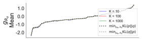
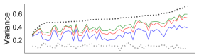
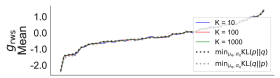
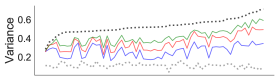
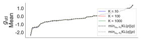
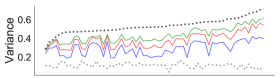
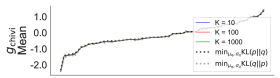
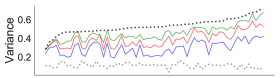
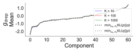
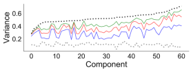
Figure 6: Optimization results for the sonar dataset ($d=61$) with all estimators.

fig:end_opt_a1a    

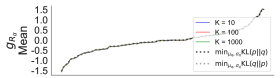
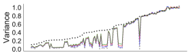
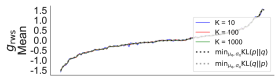
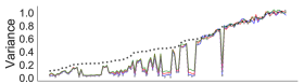
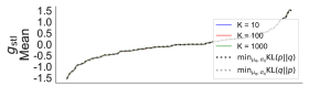
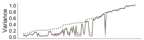
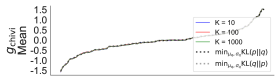
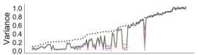
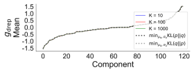
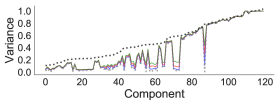
Figure 7: Optimization results for the a1a dataset ($d=120$) with all estimators.

Appendix C Weight collapse in self normalized importance sampling

This section shows the weight collapse (also known as weight degeneracy) effect of self normalized importance sampling. Simply put, the degeneracy of the normalized importance weights refers to the scenario where only a small number of samples have significant importance weight, and thus completely dominate the value of the approximations. This is known to be an inefficiency of self normalized importance sampling, since most of the samples have almost no contribution at all in the value of the estimates (Bengtsson et al., 2008).

We consider the same setting as the one in Section 2.1. We set $p$ to be a diagonal $d$-dimensional Gaussian with mean zero and variances $\sigma_{p_{i}}^{2}=0.2+9.8\frac{i}{d}$ ($i=1,...,d$), and we set $q$ to be an isotropic Gaussian with mean zero and covariance $\sigma_{q}^{2}I$, with $\sigma_{q}^{2}=9$ (its value at initialization). The normalized importance weights are computed as

$$\tilde{w}_{k}=\frac{\frac{p(x,z_{k})}{q(z_{k})}}{\sum_{j=1}^{K}\frac{p(x,z_{j})}{q(z_{j})}}\qquad\mbox{where}\qquad z_{k}\sim q.$$

We compute the normalized importance weights for several dimensions $d$ and number of samples $K$. Fig. LABEL:fig:wc shows the results. Specifically, it shows the values of the ten largest normalized weights for all the pairs $(d,K)$ considered. It can be observed that, for a dimensionality $d\geq 100$, almost all of the mass is concentrated in the largest two weights, regardless of the value of $K$ used (i.e. the weights “collapse”). This is exactly aligned with the failures observed in Section 2.1.

fig:wc            

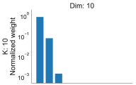
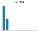
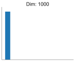
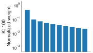
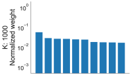
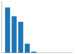
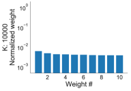
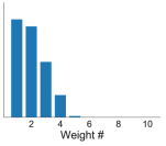
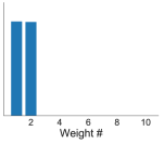
Figure 8: Visualization of the weight collapse effect of self normalized importance sampling.

References

- Bengtsson et al. (2008) Thomas Bengtsson, Peter Bickel, Bo Li, et al. Curse-of-dimensionality revisited: Collapse of the particle filter in very large scale systems. In Probability and statistics: Essays in honor of David A. Freedman, pages 316–334. Institute of Mathematical Statistics, 2008.
- Bornschein and Bengio (2014) Jörg Bornschein and Yoshua Bengio. Reweighted wake-sleep. arXiv preprint arXiv:1406.2751, 2014.
- Bugallo et al. (2017) Monica F Bugallo, Victor Elvira, Luca Martino, David Luengo, Joaquin Miguez, and Petar M Djuric. Adaptive importance sampling: the past, the present, and the future. IEEE Signal Processing Magazine, 34(4):60–79, 2017.
- Burda et al. (2016) Yuri Burda, Roger Grosse, and Ruslan Salakhutdinov. Importance weighted autoencoders. In Proceedings of the International Conference on Learning Representations, 2016.
- Carpenter et al. (2017) Bob Carpenter, Andrew Gelman, Matthew D Hoffman, Daniel Lee, Ben Goodrich, Michael Betancourt, Marcus Brubaker, Jiqiang Guo, Peter Li, and Allen Riddell. Stan: A probabilistic programming language. Journal of statistical software, 76(1), 2017.
- Dieng et al. (2017) Adji Bousso Dieng, Dustin Tran, Rajesh Ranganath, John Paisley, and David Blei. Variational inference via upper bound minimization. In Advances in Neural Information Processing Systems, pages 2732–2741, 2017.
- Domke and Sheldon (2018) Justin Domke and Daniel R Sheldon. Importance weighting and variational inference. In Advances in neural information processing systems, pages 4470–4479, 2018.
- Finke and Thiery (2019) Axel Finke and Alexandre Thiery. On importance-weighted autoencoders. arXiv preprint arXiv:1907.10477, 2019.
- Geffner and Domke (2020) Tomas Geffner and Justin Domke. On the difficulty of unbiased alpha divergence minimization. arXiv preprint arXiv:2010.09541, 2020.
- Kingma and Ba (2014) Diederik P Kingma and Jimmy Ba. Adam: A method for stochastic optimization. arXiv preprint arXiv:1412.6980, 2014.
- Kingma and Welling (2013) Diederik P Kingma and Max Welling. Auto-encoding variational bayes. In Proceedings of the International Conference on Learning Representations, 2013.
- Kuleshov and Ermon (2017) Volodymyr Kuleshov and Stefano Ermon. Neural variational inference and learning in undirected graphical models. In Advances in Neural Information Processing Systems, pages 6734–6743, 2017.
- Li and Turner (2016) Yingzhen Li and Richard E Turner. Rényi divergence variational inference. In Advances in Neural Information Processing Systems, pages 1073–1081, 2016.
- Maddison et al. (2017) Chris J Maddison, John Lawson, George Tucker, Nicolas Heess, Mohammad Norouzi, Andriy Mnih, Arnaud Doucet, and Yee Teh. Filtering variational objectives. In Advances in Neural Information Processing Systems, pages 6573–6583, 2017.
- Naesseth et al. (2020) Christian A Naesseth, Fredrik Lindsten, and David Blei. Markovian score climbing: Variational inference with kl. arXiv preprint arXiv:2003.10374, 2020.
- Neal (2011) Radford M Neal. Mcmc using hamiltonian dynamics. Handbook of markov chain monte carlo, 2(11):2, 2011.
- Roeder et al. (2017) Geoffrey Roeder, Yuhuai Wu, and David K Duvenaud. Sticking the landing: Simple, lower-variance gradient estimators for variational inference. In Advances in Neural Information Processing Systems, pages 6925–6934, 2017.
- Titsias and Lázaro-Gredilla (2014) Michalis Titsias and Miguel Lázaro-Gredilla. Doubly stochastic variational bayes for non-conjugate inference. In Proceedings of the 31st International Conference on Machine Learning (ICML-14), pages 1971–1979, 2014.
- Tran et al. (2016) Dustin Tran, Alp Kucukelbir, Adji B Dieng, Maja Rudolph, Dawen Liang, and David M Blei. Edward: A library for probabilistic modeling, inference, and criticism. arXiv preprint arXiv:1610.09787, 2016.
- Tucker et al. (2018) George Tucker, Dieterich Lawson, Shixiang Gu, and Chris J Maddison. Doubly reparameterized gradient estimators for monte carlo objectives. arXiv preprint arXiv:1810.04152, 2018.