Mapping of Dynamics between Mechanical and Electrical Ports in SG-IBR Composite Grids

Abstract

Power grids are traditionally dominated by synchronous generators (SGs) but are currently undergoing a major transformation through the increasing integration of inverter-based resources (IBRs). The SG-dominated grid is traditionally analyzed in a mechanical-centric view which ignores fast electrical dynamics and focuses on the torque-speed dynamics. By contrast, analysis of the emergent IBR-dominated grid usually takes the electrical-centric view which focuses on the voltage-current interaction. In this article, a port-mapping method is proposed to fill the gap between these approaches and combine them in a unified model. Specifically, the mechanical dynamics are mapped to the electrical impedance seen at the electrical port; and the electrical dynamics are also mapped to the torque coefficient seen at the mechanical port. The bidirectional mapping gives additional flexibility and insights to analyze the sub-system interactions in whole-system dynamics and guide the tuning of parameter. Application of the proposed method is illustrated in three cases with increasing scales, namely a single-SG-infinite-bus system, a single-IBR-weak-grid system, and a modified IEEE 14-bus SG-IBR composite system.

I Introduction

Power systems have traditionally been dominated by synchronous generators (SGs) [1, 2]. In recent years, due the drive towards renewable energy, power electronics and inverter-based resources (IBRs) have become increasingly common features of the power system [3, 4, 5], and thus the power system is being transformed from SG-dominated to SG-IBR composite. This structural change results in new oscillation modes and the emergence of new stability problems [5, 6, 7, 8].

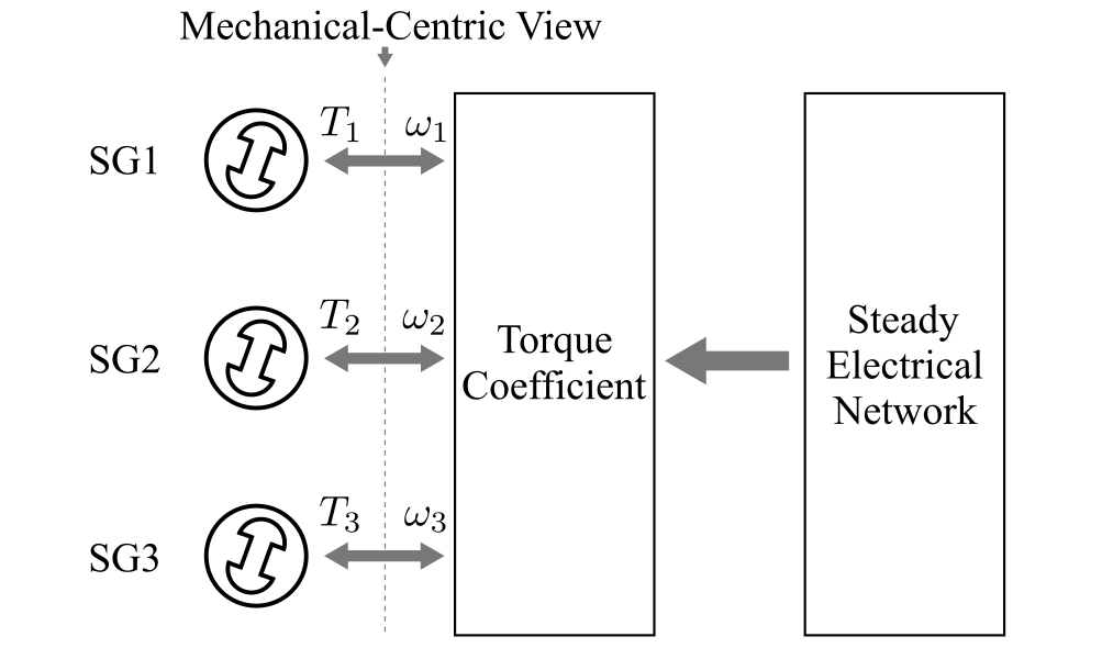
(a)

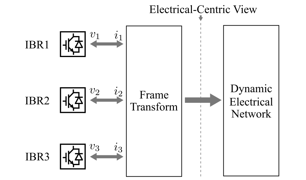
(b)

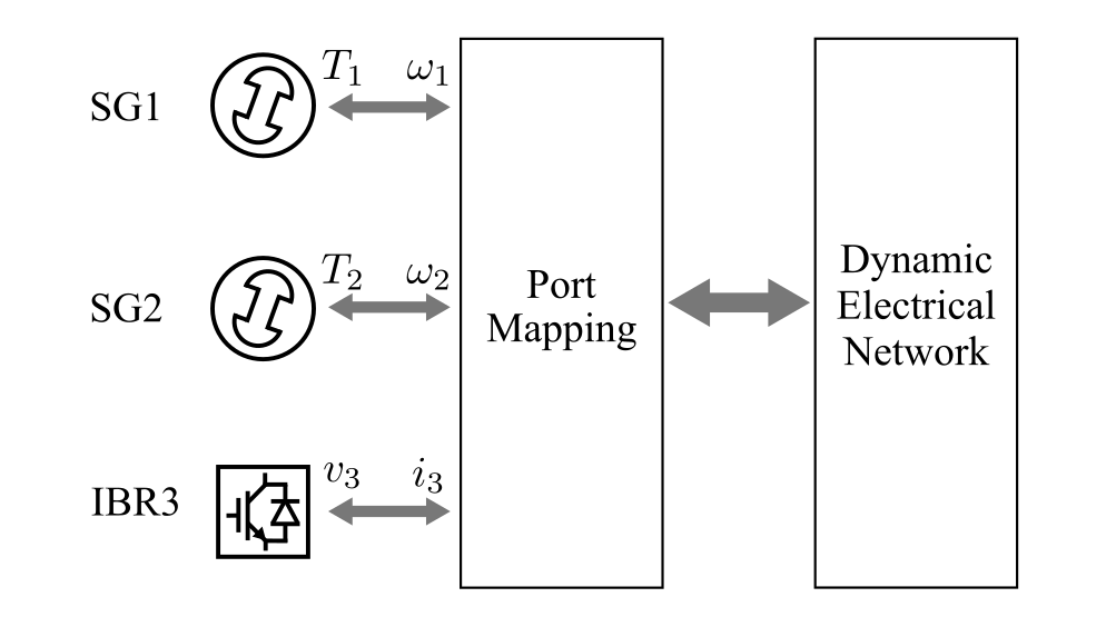
(c)

Figure 1: Power system analysis framework. (a) Mechanical-centric view of SG-dominated systems, where $T$ and $\omega$ are torque and rotor speed respectively. (b) Electrical-centric view of IBR-dominated power systems, where $v$ and $i$ are voltage and current respectively. (c) Port-mapping view of SG-IBR composite power systems.

Modeling the system dynamics is the first step to addressing the emerging challenges to system stability. One fundamental challenge for an SG-IBR composite grid is that different modeling frameworks have been adopted and evolved for SGs and IBRs. For an SG-based grid, a mechanical-centric perspective has been adopted: the speed and rotor angle of synchronous generators are selected as state variables, and the behavior of the grid is considered in terms of the torque-speed ($T$-$\omega$) interaction between the SGs that transfer power via the power flow on transmission lines. For this perspective, the electrical network is transformed to a mechanical representation as torque coefficients, as illustrated in Fig. 1 (a) [1]. This perspective has been very successful for SG dominated grids, but the fast electrical dynamics of the network are neglected when transformed to torque coefficients, meaning that it is not applicable when fast electromagnetic transients (EMTs) are of concern.

In contrast, modelling of an IBR-based grid usually takes an electrical-centric perspective in which voltages and currents are the focus of the model. The behavior of the grid is represented by the voltage-current ($v\text{-}i$) interaction between the IBRs and the network, as shown in Fig. 1 (b) [9, 10, 11, 12, 13]. This approach preserves all electrical dynamics of IBRs, but it is not straightforward to represent the mechanical dynamics of SGs (torque, speed, and inertia of the rotor) by using the electrical variables (the voltage and current of the stator). Therefore, this method was normally used for super-synchronous (or harmonic) analysis where the synchronization (governed by the rotation of mechanical angles) is not of concern.

It is clear that neither approach fully models an SG-IBR composite grid where both EMT and rotational synchronisation make important contributions to whole-system stability of the power system. Therefore, a framework that can unite the mechanical- and electrical-centric views is highly desired. The fundamental difficulty in establishing a unified view is that frame transformations are needed to align the mechanical angles of the various SGs (as well as the phase-locked angles of the various IBRs) in the dynamic electrical network. The frame transformations themselves contain dynamics meaning that SG and IBR in different frames cannot be directly connected [14]. To address this difficulty, a method called frame dynamics embedding is proposed in [15] where the rotational dynamics in the frame transformation are embedded into electrical models in order that frame transformations do not need separate treatment of dynamics. The frame dynamics embedding method is applied to both SGs and IBRs, yielding impedance element models where the mechanical rotors and the phase-locked loops are represented as equivalent electrical elements [15, 13, 16]. This representation points the way towards a possible unified mechanical-electrical modelling framework capable of predicting the interaction between swing dynamics and inductance dynamics in low-inertia grids.

In this paper, we proposed an inverse approach to the frame dynamics embedding method in [15] by transforming the electrical dynamics back to the mechanical-centric view. This approach yields a dynamic torque coefficient which includes EMT features on top of the classic torque coefficient. The dynamic torque coefficient provides a natural interpretation of IBR-SG interaction from the mechanical viewpoint such that the established concepts and terminology for SG-dominated grids can still be used for grids with high-penetration of IBRs and fast electrical dynamics. The proposed approach, combined with the frame dynamics embedding method, completes the picture of a unified mechanical-electrical view. It is named the port-mapping method in this article because it bidirectionally maps dynamics across mechanical and electrical ports, as illustrated in Fig. 1 (c). The port-mapping method can also be generalised to other ports, such as the dc-links in IBRs or the exciters in SGs.

The paper is organized as follows. In Section II, the concept of port-mapping is introduced and the detailed modelling procedure is illustrated on a SG and a IBR. Section III links the port-based models in a SG-IBR composite grid to show the extra flexibility and insights provided by the proposed method in system dynamic analysis. Section IV demonstrated the proposed method in three case studies. Section V concludes the paper.

II The Port-Mapping Method

In this section, we introduce the fundamentals of the port-mapping method via the examples of a SG and an IBR.

II-A Mechanical-Electrical Two-Port Network

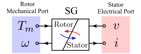
(a)

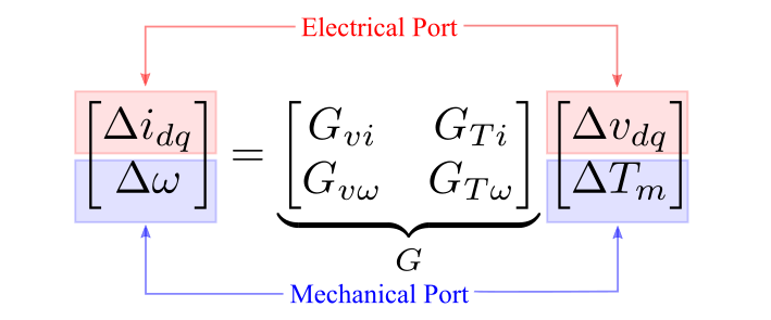
(b)

Figure 2: Two-port model of SG. (a) Port-mapping flow. (b) Transfer function model.

Inspired by the two-port network theory in electrical circuits [17], we represent a SG as a mechanical-electrical two-port model as shown in Fig. 2. The mechanical port captures the mechanical dynamics between mechanical torque $T_{m}$ and rotor speed $\omega$ through the rotor shaft, and the electrical port captures the electrical dynamics between terminal voltage $v$ and current $i$ through stator windings. The two ports interact with each other via electrical-mechanical coupling between the rotor and the stator. The mathematical description of the mechanical-electrical two-port network can be formulated as a transfer function matrix $G$ whose diagonal elements represent the self dynamics of a port and the off-diagonal elements represent cross-port coupling, as illustrated in Fig. 2 (b). The matrix can be readily obtained by linearizing the state equations of a SG as described in Appendix A.

The mechanical-electrical two-port model provides a general step for cross-domain modelling but there are difficulties to overcome before these modular models can be used in whole-system analysis. The model of a SG is presented in its local $dq$ reference frame aligned to its rotor, which needs to be aligned to a global reference frame $DQ$ when the electrical ports of multiple apparatuses are linked in a grid. The frame alignment contains dynamics in itself which is usually represented as extra global synchronising signals, making the linked whole-system model lose modularity. To solve this problem, we transform the electrical port to the global $DQ$ frame and map the frame dynamics into the port matrix so that no extra global synchronisation signals are needed and the whole-system model retains modularity, as described in the following sub-section.

II-B Mechanical Dynamics Mapping to Electrical Ports

Our approach is based on the key observation that the mechanical dynamics of the rotor is identical to the frame dynamics of the electrical port, which offer a bridge for dynamic mapping across mechanical-electrical ports, as illustrated conceptually in the port-mapping flow in Fig. LABEL:Fig:SingleMachineInfiniteBus (c) and shown in detail in the block diagram in Fig. LABEL:Fig:SingleMachineInfiniteBus (e). We now give the mathematical details. The transformation from mechanical frame $dq$ to global frame $DQ$ for an arbitrary signal $u$ can be represented using the transformation matrix $T_{\epsilon}$ as

$$\underbrace{\begin{bmatrix}u_{D}\\ u_{Q}\end{bmatrix}}_{u_{DQ}}=\underbrace{\begin{bmatrix}\cos{\epsilon}&-\sin{\epsilon}\\ \sin{\epsilon}&\cos{\epsilon}\end{bmatrix}}_{T_{\epsilon}}\underbrace{\begin{bmatrix}u_{d}\\ u_{q}\end{bmatrix}}_{u_{dq}}$$ (1)

where $\epsilon$ is the angle difference between $dq$ and $DQ$ as indicated in Fig. LABEL:Fig:SingleMachineInfiniteBus (a). By linearizing this equation, we get

$$\underbrace{\begin{bmatrix}\Delta u_{D}\\ \Delta u_{Q}\end{bmatrix}}_{\Delta u_{DQ}}=T_{\epsilon_{0}}\bigg{(}\underbrace{\begin{bmatrix}\Delta u_{d}\\ \Delta u_{q}\end{bmatrix}}_{\Delta u_{dq}}+\underbrace{\begin{bmatrix}-u_{q0}\\ u_{d0}\end{bmatrix}}_{U_{0}}\Delta\epsilon\bigg{)}$$ (2)

where the subscript $0$ denotes steady-state operating points and the prefix $\Delta$ denotes perturbation around the operating points. The angle perturbation $\Delta\epsilon$ is the integration of the mechanical speed, that is, $\Delta\epsilon=\Delta\omega/s$ where $s$ is Laplace operator so $1/s$ represents integration. This relationship is indicated by the blue arrows in the block diagram Fig. LABEL:Fig:SingleMachineInfiniteBus (e) and yields the transformation from $G$ to $G^{\prime}$, where the electrical port of $G^{\prime}$ is represented in the global $DQ$ frame so that it can be readily linked with other apparatuses in the electrical network. The detailed process of the transformation and the element-wise value of $G^{\prime\prime}$ can be found in Appendix B-A. The transformed $G^{\prime}$ has an identical effect to the frame-dynamic embedding method in [15] but preserves the mechanical port on top of [15] so that the bi-directional mapping between the two ports are available. This allow us to map the electrical dynamics back to mechanical ports which provide extra flexibility and insight in stability analysis, to follow.

II-C Electrical Dynamics Mapping to Mechanical Ports

In the mechanical-electrical two-port model $G^{\prime}$ the terminal voltage $v_{DQ}$ is taken as an independence input. In reality, however, $v_{DQ}$ is affected by the current $i_{DQ}$ via the equivalent impedance $Z_{b}$ seen at the bus where the apparatus is connected. This yields an extra loop in the block diagram as indicated by the red arrow in Fig. LABEL:Fig:SingleMachineInfiniteBus (e). Closing this loop yields the transformation from $G^{\prime}$ to $G^{\prime\prime}$ where the electrical impedance of the grid $Z_{b}$ is mapped into the two-port network. It should be noted that input voltage of $G^{\prime\prime}$ is changed from $v_{DQ}$ to $v_{bDQ}$ which is the equivalent voltage of the grid behind $Z_{b}$. The detailed process of the transformation and the element-wise value of $G^{\prime\prime}$ can be found in Appendix B-B.

II-D Generalising to IBR

The port-mapping methodology for a SG discussed in the previous sub-sections can be readily generalised to other apparatuses, such as an IBR, as illustrated in the right column in Fig. LABEL:Fig:SingleMachineInfiniteBus. An IBR (grid-following) has a rotating angle in its phase-locked loop (PLL) which is used for synchronisation. The active power is regulated by the balancing of the dc-link voltage. The PLL and the dc-link in a grid following IBR roughly have the same function as the rotor in a SG, for synchronisation and power balancing. Therefore, an IBR is three-port apparatus where the PLL and dc-link port jointly serve as a virtual mechanical port. The port-mapping transformation from $G$ to $G^{\prime}$ and to $G^{\prime\prime}$ for an IBR can be obtained easily from the block diagrams in Fig. LABEL:Fig:SingleMachineInfiniteBus (f).

III Port-Based Analysis of SG-IBR Composite Grids

Having established a step-by-step procedure for dynamic mapping across ports in a SG and a IBR, we now use the derived port-based model to examine the stability of SG-IBR composite grids.

III-A Linking SG-IBR Composite Grids

We first link the port-based SG and IBR models in a composite network. Taking the network in Fig. 4 as an example, the corresponding block diagram is shown in Fig. 5. The port matrix $G$ for each apparatus is transformed to $G^{\prime}$ (this is done locally without the knowledge on the whole grid), and then appended on $G_{N}^{\prime}$ to represent the collective port matrices of all apparatuses. $G^{\prime}_{N}$ interact with the network impedance matrix $Z_{bN}$ to form the whole-system port model $G_{N}^{\prime\prime}$. $Z_{bN}$ is the inversion of nodal admittance matrix $Y_{bN}$ [15] rather than a simple branch impedance. $Z_{b}$ is dynamic impedance formulated in the $s$-domain (not simply $R+jX$) so all EMT dynamics are preserved. The entire procedure for port-mapping and port-based modelling are summarized in the model derivation tree in Fig. 6 for a clearer review.

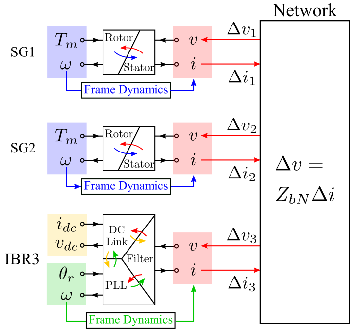
Figure 4: Port-mapping flow for a SG-IBR Composite power network.

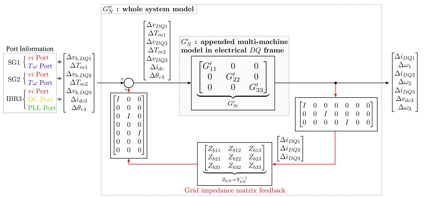
Figure 5: Block diagram for the SG-IBR composite power network in Fig. 4.

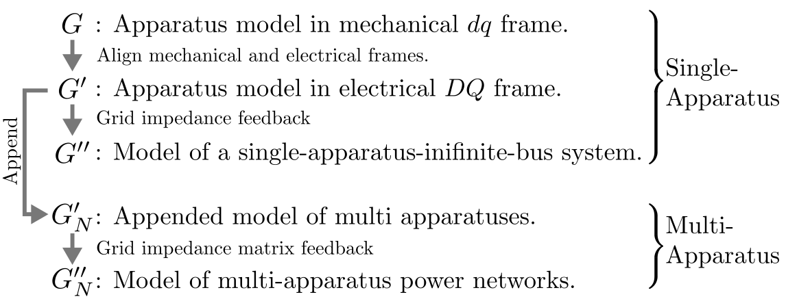
Figure 6: Model derivation tree: the procedure to get single-apparatus and multi-apparatus port matrices.

III-B Port-Based System Bipartition

Now we explain the benefits of the port-mapping approach in whole-system stability studies. System bipartition is commonly used to investigate the interaction of sub-systems in a power system. For example, in the electrical-centric view, a power system is separated into sources and loads and their interaction is characterised by the impedance ratio between the source part and load part. This bipartition method can be naturally generalized in the port-based approach which turns out to provide additional flexibility in analyzing dynamic interaction from different views (mechanical-centric and electrical-centric).

For instance, we can split the system in Fig. 7 at the $T\text{-}\omega$ (mechanical) port of SG1. The transfer function seen at this port is ${G_{T\omega 11}^{\prime\prime}}$. We take out the rotor inertia from this port and model the dynamics the rest parts of the grid as a dynamic torque coefficient $K_{T1}$

$$K_{T1}={G_{T\omega 11}^{\prime\prime\,-1}}-sJ_{1}.$$ (3)

The stability of the system is boiled down to the closed-loop interaction between rotor inertia $\frac{1}{sJ_{1}}$ and the dynamic torque coefficient $K_{T1}$, as shown in Fig. 7. $K_{T1}$ is an extension to the classic torque coefficient and it encodes the dynamics of the entire grid (including EMT) except the rotor of SG1. If $K_{T1}$ itself is stable, the whole-system stability can be evaluated by the loop gain of Fig. 7 via Nyquist criterion. Since $\frac{1}{sJ_{1}}$ has a constant phase shift of $-90^{\circ}$ along the Nyquist contour, the phase of $K_{T1}$ should be kept above $-90^{\circ}$ to ensure positive phase margin, which leads to a very simple stability index.

Similarly, we can also split the system in Fig. 7 at the $i_{dc}\text{-}v_{dc}$ (dc-link) port of IBR3. We define the dc-link capacitance as the electrical inertia and takes it out from the port transfer function $G_{i_{dc}v_{dc}33}^{\prime\prime}$ to yield the closed-loop diagram in Fig. 8 where

$$K_{i_{dc}3}={G_{i_{dc}v_{dc}33}^{\prime\prime\,-1}}-sC_{3}$$ (4)

is called the dc-current coefficient. $K_{i_{dc}3}$ plays a similar role to $K_{T1}$ which are named generalised torque coefficient together.

It is possible to explore other ways of bipartition at different ports, e.g. an exciter port of a SG, or a $V\text{-}Q$ control port of an IBR. The port under investigation can be select to the point where oscillations stand out to provide insightful interpretations right on the spot. We can also split multiple ports simultaneously to investigate oscillations in which multiple apparatuses are participating.

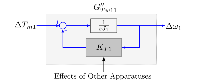
Figure 7: The bipartite system viewed from mechanical port of SG1.

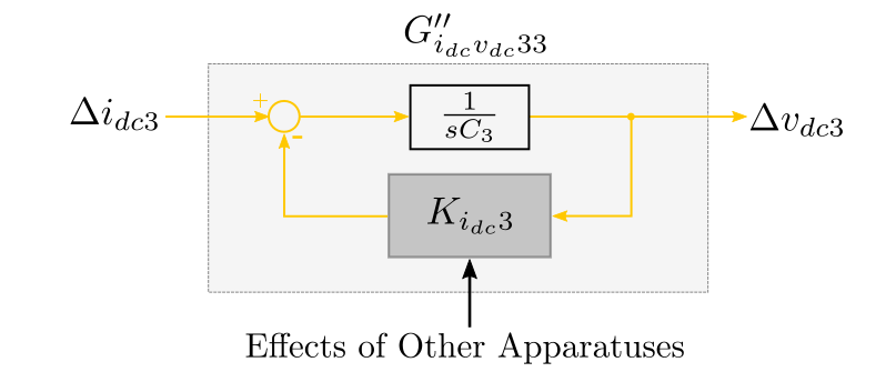
Figure 8: The bipartite system viewed from dc-link port of IBR3.

III-C Practical Implementation

The port-based method proposed in this paper can be formulated in either state-space or transfer-function format, although we use transfer functions in our formulation, mainly for brevity in illustration. Inspire by the widely used open-source tools which automate system analysis work flow [18, 19, 20], we developed our own open-source toolbox to automate the proposed port-based stability analysis [21]. User only need to input a simple table specifying network layout and apparatus parameters, and the toolbox assemble the port-based whole-system model and visualise the stability results in time domain and frequency domain in just one click. The assembled models are graphically presented as Simulink block diagrams.

As pointed out in Section II-B, the proposed port-mapping method eliminates the global synchronisation signals (maps them into ports) and thus is a completely modular approach. Modular stabilization techniques, such as the passivity-based method [22, 11], scale-free synthesis [23], and port-Hamilton method [24], can thus be easily incorporated in our port-based model. By contrast, prior-art component connection model [14] cannot directly makes use of these techniques as the global synchronisation signals break modularity.

IV Case Studies

In this section, the effectiveness of port-mapping modeling is illustrated through analyzing system stability in three cases. The first two case, (a) single-SG-infinite-bus system and (b) single-IBR-weak-grid system revisit well-known stability concerns in very simple set-ups but with new insights. The third case, (c) modified IEEE 14-bus SG-IBR composite system, illustrates modelling of composite systems. The parameters and models of all three cases, generated from the procedures in Section II and Section III, are available at [21].

IV-A Case 1: Single-SG-Infinite-Bus System

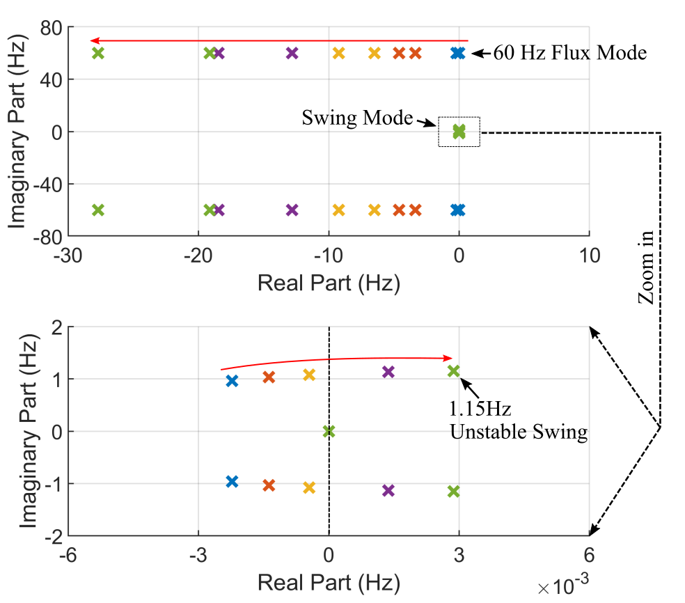
Figure 9: Case 1: whole-system pole locus with increasing $R_{b}$ from 0 pu to 0.3 pu.

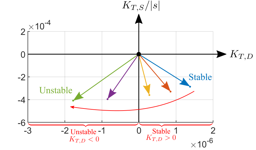
Figure 10: Case 1: vector diagram of torque coefficient $K_{T}$ when increasing the line resistance from 0 pu to 0.3 pu.

A single-SG-infinite-bus system and the familiar swing-dynamics are used to illustrate the effect of changing the damping at the stator electrical port, i.e., the line resistance $R_{b}$, on the dynamics at the rotor mechanical port. The poles of whole-system model $G_{N}^{\prime\prime}$ are shown in Fig. 9 including a sweep of $R_{b}$ from 0 pu to 0.3 pu. The 60 Hz electrical flux modes are damped and shifted leftward when $R_{b}$ increases, as expected because $R_{b}$ is in series with the inductor of the relevant flux. The zoomed-in pole locus in the lower part of Fig. 9 shows that the swing modes, in contrast, move to rightward: the increase of electrical damping through $R_{b}$ decreases the damping of the swing oscillation, i.e., decreases the mechanical damping, eventually causing instability when the SG’s own damping coefficient $K_{D}$ is inadequate (at 0.2 pu here). This can be further examined using the port bipartition method in Fig. 7 by calculating the torque coefficient $K_{T}$ inclusive of network effects. As shown in Fig. 10, as $R_{b}$ is increased from 0 pu to 0.3 pu, the vector $K_{T}$ moves into the third quadrant with its phase decreasing to $<-90^{\degree}$ which implies negative $K_{T,D}$ and an unstable swing. This variation in the angle of $K_{T}$ with $R_{b}$ is an example of translating the grid impedance into the torque coefficient through the bidirectional mapping of dynamics between electrical and mechanical ports, as discussed in theoretical terms in Section II-C. Here, increasing the positive electrical damping (line resistance $R_{b}$) is seen to map to a decreased mechanical damping (decreased dynamic damping torque coefficient $K_{T,D}$). This also implies that increasing the self mechanical damping of the SG can re-stabilize this oscillation as tested next.

The time-domain simulation results of Fig. 11 confirm that when line resistance $R_{b}$ is increased from 0 pu to 0.3 pu at $0~{}s$ leads to a 1.15 Hz swing oscillation which is damped when at 5 s, the mechanical damping $K_{D}$ of the SG is increased from 0.2 pu to 2 pu.

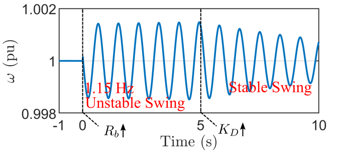
Figure 11: Case 1: simulation results of SG dynamics. At 0 s, line resistance $R_{b}$ is increased from 0 pu to 0.3 pu which destabilizes the swing mode. At 5 s, $K_{D}$ of SG is increased from 0.2 pu to 2 pu which re-stabilizes the swing mode.

IV-B Case 2: Single-IBR-Weak-Grid System

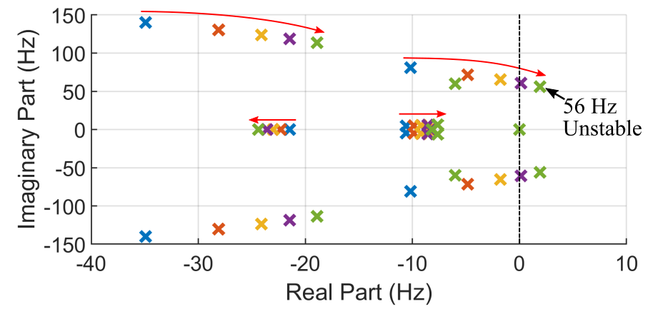
Figure 12: Case 2: whole-system pole locus when reducing the SCR from 2.71 to 1.35.

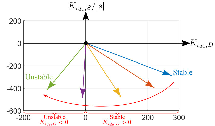
Figure 13: Case 2: vector diagram of dc-current coefficient $K_{i_{dc}}$ when reducing the SCR from 2.71 to 1.35.

It is known that the stability of a grid-following IBR is degraded when connected to a weak grid, i.e., a grid with large impedance and low short-circuit ratio (SCR) [25]. The port-separation method will again be used to identify how changed at the ac electrical port mapped to the dc-link port. The whole-system pole map in Fig. 12 illustrates that when the SCR was reduced from 2.71 to 1.35, the 56 Hz mode became unstable. The plot of the dc-current coefficient vector $K_{i_{dc}}$ in Fig. 13 reveals the same onset of instability as a change in the angle of the vector. In this case, the changed dynamics caused by the high line impedance (low SCR) at the ac electrical port are seen to be mapped to the dc-current coefficient at dc electrical port of the IBR. This confirms that the port-mapping and port-separation methods can represent and reveal causes of IBR instability.

The time-domain simulation results of Fig. 14 confirm that when the gird is weakened with SCR reduced from 2.71 to 1.35 at 0 s, a 56 Hz unstable oscillation begins. At 0.1 s, SCR is increased back to 2.71, which re-stabilizes the system.

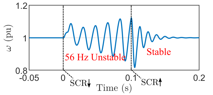
Figure 14: Case 2: simulation results of IBR dynamics. At 0 s, SCR is reduced from 2.71 to 1.35 which leads to the instability. At 0.1 s, SCR is increased back to 2.71 which re-stabilizes the system.

IV-C Case 3: Modified IEEE 14-Bus SG-IBR Composite System

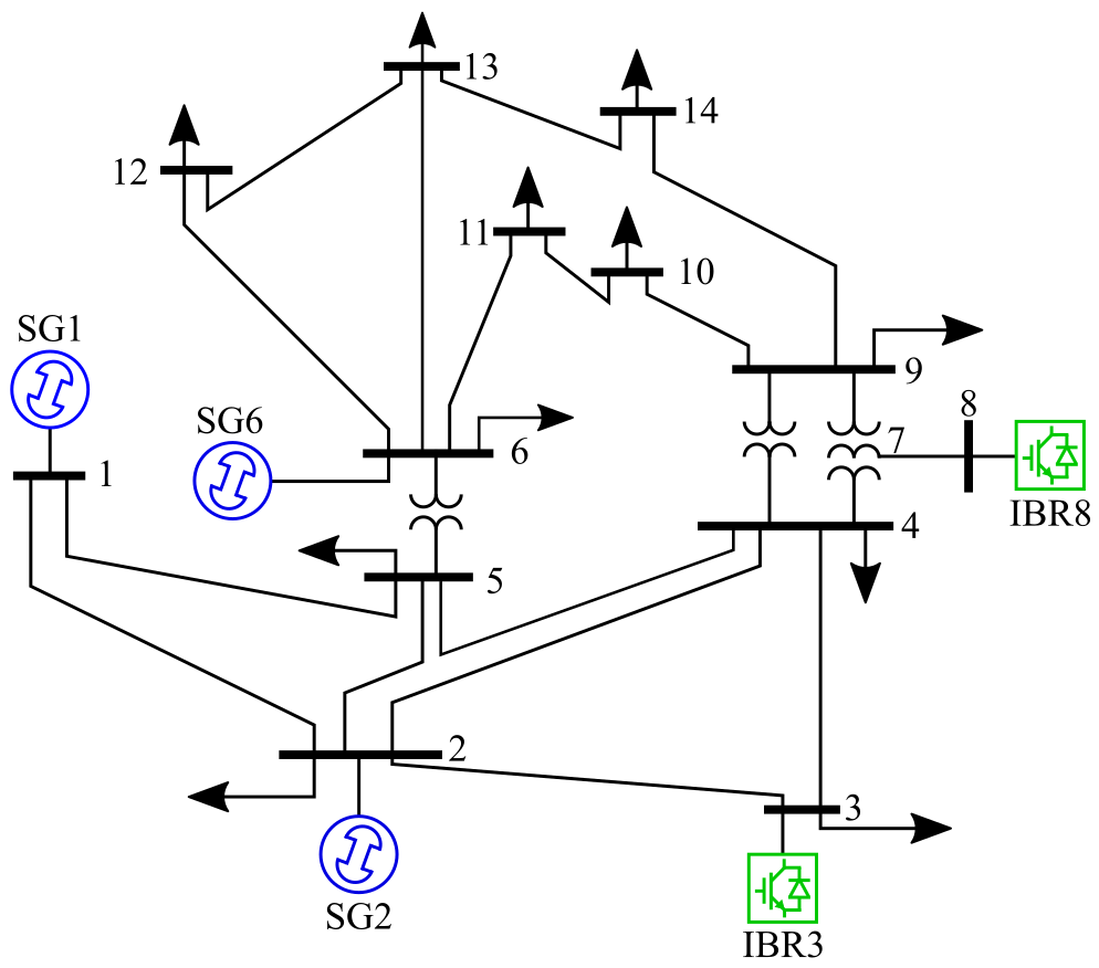
Figure 15: Case 3: IEEE 14-bus SG-IBR composite power system.

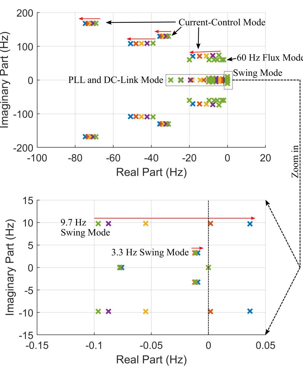
Figure 16: Case 3: whole-system pole locus with reducing the IBR power-frequency-related control bandwidth (dc-link and PLL) from 25 Hz to 5 Hz.

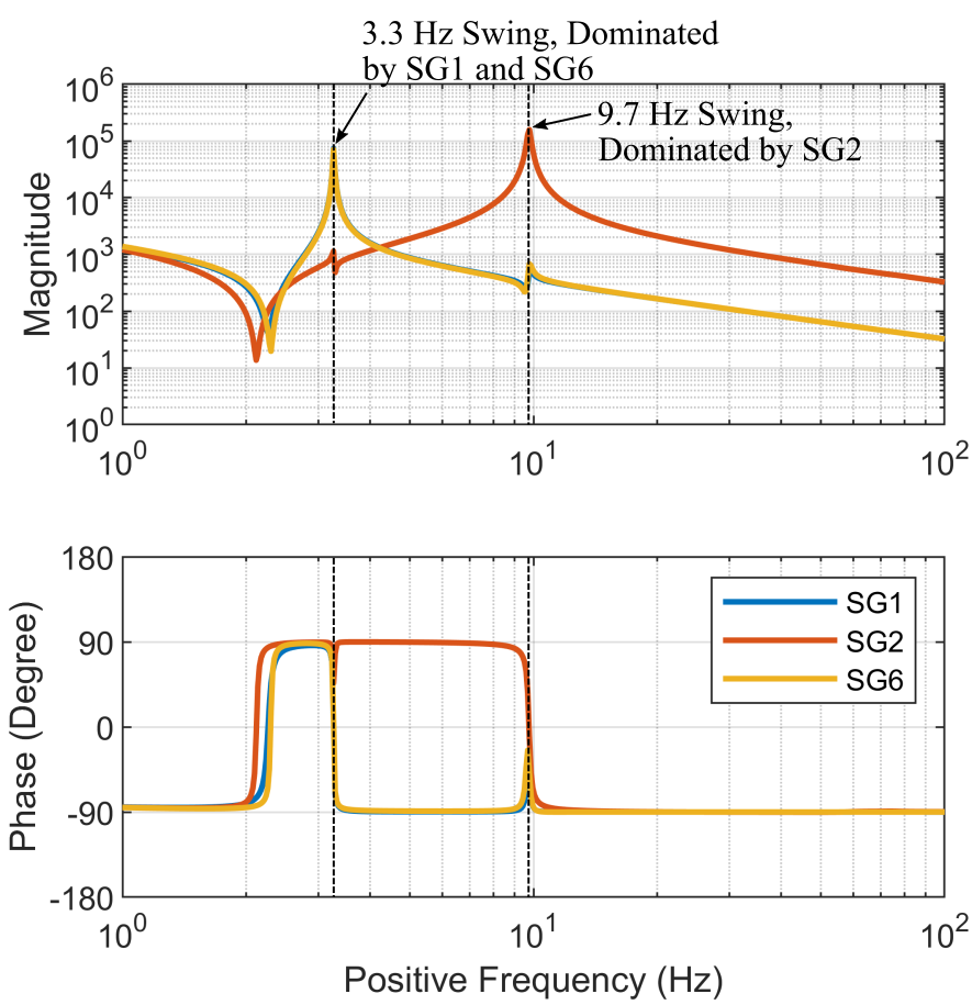
Figure 17: Case 3: Bode diagram of $T\omega$ port closed-loop transfer function (i.e., the mechanical impedance $G_{T\omega}^{\prime\prime}$ in $G_{N}^{\prime\prime}$) for each SG.

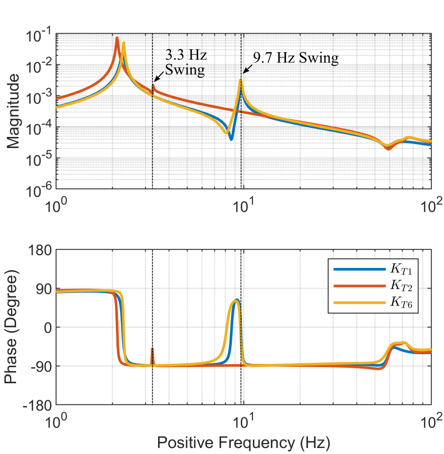
(a)

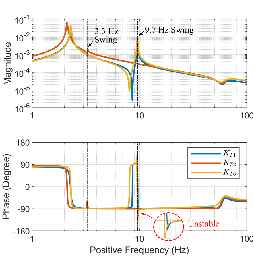
(b)

Figure 18: Case 3: Bode diagram of torque coefficient $K_{T}$ for each SG with changing the power-frequency control bandwidth (dc-link and PLL) of IBRs. (a) Bandwidth of 25 Hz. (b) Bandwidth of 5 Hz.

To analyze the power-frequency interaction between SGs and IBRs, a modified IEEE 14-bus power system is investigated next, as shown in Fig. 15. The same layout of the IEEE standard 14-bus system is retained but two SGs are replaced by IBRs. Fig. 16 shows the poles of the whole system when bandwidth of the power-frequency controllers (i.e., dc-link and PLL) of the IBRs are reduced from 25 Hz to 5 Hz. The zoomed-in figure shows the loci of the swing modes. These can be classified into two groups: stable 3.3 Hz poles and unstable 9.7 Hz poles. The magnitude of resonant peak of closed-loop gain $G_{T\omega}^{\prime\prime}$ for each SG in Fig. 17 reveals the participation of apparatuses on oscillation modes [26]. It indicates that the 9.7 Hz swing mode is dominated by SG2 (red line), and the 3.3 Hz swing mode is jointly dominated by SG1 (blue line) and SG6 (yellow line). The port-separation method can be used here to obtain the torque coefficient $K_{N}$ of each SG, as shown in Fig. 18, where the bode plot is used here so that we can investigate the magnitude and phase of the torque coefficient vectors at both swing mode frequencies in same figure. Results for control bandwidths of 25 Hz are in (a) and 5 Hz in (b). A phase of $K_{T}$ smaller than $-90^{\degree}$ can be observed at the 9.7 Hz swing point for bandwidth of 5Hz which agrees with the pole loci.

The corresponding time-domain simulation results are shown in Fig. 19. At 0 s, the IBR power-frequency bandwidth is reduced from 25 Hz to 5 Hz and the unstable 9.7 Hz swing oscillation begins. At 5 s, the damping torque coefficient $K_{D2}$ of the critical SG2 is increased from 1 pu to 2 pu, which re-stabilizes the system.

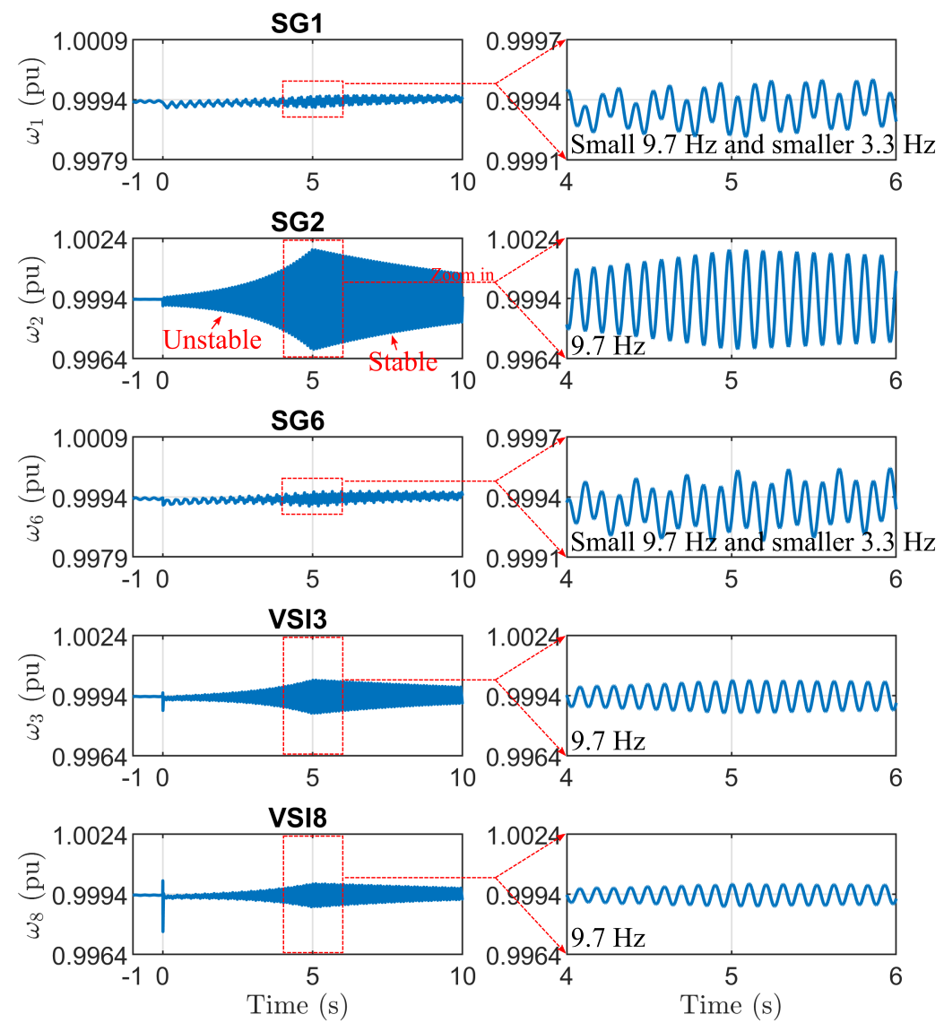
Figure 19: Case 3: simulation results. At 0 s, the power-frequency control bandwidth of IBR (dc-link and PLL) is reduced from 25 Hz to 5 Hz, which destabilizes the 9.7 Hz swing mode. At 5 s, the damping torque coefficient $K_{D2}$ of SG2 is increased from 1 pu to 2 pu, which re-stabilizes the system.

V Conclusions

A port-mapping method has been put forward for stability analysis of composite power systems with mixtures of SGs and IBRs. The proposed method maps the dynamics between multi-physical-domain ports and gives more insights on whole system stability. It unifies the mechanical- and electrical-centric analysis of power systems in a single model. The mechanical rotational dynamics are mapped to the electrical impedance or admittance, and meanwhile the electrical dynamics are also mapped to the mechanical torque coefficient. This united cross-domain methodology enables more flexible bipartition of power systems to allow for more interpretative investigation into the interaction amongst sub-systems, which yields new stability indices such as generalised torque coefficients.

Appendix A State Equations of Synchronous Generator

State equations of a SG with considering both stator electrical dynamics and rotor mechanical dynamics (in source convention) are [1, 15]

$$v_{d} =\dot{\psi}_{d}-Ri_{d}-\omega\psi_{q}$$ (5)

$$v_{q} =\dot{\psi}_{q}-Ri_{q}+\omega\psi_{d}$$

$$J\dot{\omega} =T_{m}-T_{e}-K_{D}{\omega}$$

with

$$\psi_{d}=-Li_{d},~{}\psi_{q}=-Li_{q}-\psi_{f},~{}T_{e}=\psi_{f}i_{d}$$ (6)

where $\psi_{d}$ and $\psi_{q}$ are $dq$-axis flux linkages respectively; $\psi_{f}$ is the field flux linkage; $v_{d}$ and $v_{q}$ are $dq$-axis stator voltages; $i_{d}$ and $i_{q}$ are $dq$-axis stator currents; $\omega$ is the rotor speed; $J$ is the rotor inertia; $T_{m}$ and $T_{e}$ are the mechanical and electromagnetic torque respectively; $K_{D}$ is the damping torque coefficient; $R$ and $L$ are stator resistance and inductance respectively.

Appendix B Model Derivation of Port-Mapping Method

B-A $G$ (Mechanical Frame) $\rightarrow$ $G^{\prime}$ (Global Frame)

According to Fig. LABEL:Fig:SingleMachineInfiniteBus (e), the element relationship between $G$ (mechanical frame) and $G^{\prime}$ (electrical frame) can be obtained as

$$G_{vi}^{\prime}=T_{\epsilon_{0}}\bigg{(}G_{vi}+(I_{0}-G_{vi}V_{0})\underbrace{(s+G_{v\omega}V_{0})^{-1}G_{v\omega}}_{G_{v\omega}^{\prime}T_{\epsilon_{0}}/s}\bigg{)}T_{\epsilon_{0}}^{-1}$$ (7)

$$G_{Ti}^{\prime}=T_{\epsilon_{0}}\bigg{(}G_{Ti}+(I_{0}-G_{vi}V_{0})\underbrace{(s+G_{v\omega}V_{0})^{-1}G_{T\omega}}_{G_{T\omega}^{\prime}/s}\bigg{)}$$

$$G_{v\omega}^{\prime}=\bigg{(}s(s+G_{v\omega}V_{0})^{-1}G_{v\omega}\bigg{)}T_{\epsilon_{0}}^{-1}$$

$$G_{T\omega}^{\prime}=s(s+G_{v\omega}V_{0})^{-1}G_{T\omega}$$

where $I_{0}=[-i_{q0};i_{d0}]$ and $V_{0}=[-v_{q0};v_{d0}]$ are the steady-state operating points at the electrical port; $T_{\epsilon_{0}}$ is the frame transformation matrix with the steady-state angle $\epsilon_{0}$. The first equation in (7) builds the relationship between $G_{vi}$ (admittance in mechanical frame) and $G_{vi}^{\prime}$ (admittance in electrical frame), which correspond to the impedance-based analysis in [15, 16] albeit that they focus on the electrical domain only.

B-B $G^{\prime}$ (Apparatus Model) $\rightarrow$ $G^{\prime\prime}$ (Whole System Model)

According to Fig. LABEL:Fig:SingleMachineInfiniteBus (e), the element relationship between $G^{\prime}$ (apparatus model) and $G^{\prime\prime}$ (whole system model for the single-SG-infinite-bus system) can be obtained as

$$G_{vi}^{\prime\prime}=(I-G_{vi}^{\prime}Z_{b})^{-1}G_{vi}^{\prime}$$ (8)

$$G_{Ti}^{\prime\prime}=(I-G_{vi}^{\prime}Z_{b})^{-1}G_{Ti}^{\prime}$$

$$G_{v\omega}^{\prime\prime}=G_{v\omega}^{\prime}+G_{v\omega}^{\prime}Z_{b}\underbrace{(I-G_{vi}^{\prime}Z_{b})^{-1}G_{vi}^{\prime}}_{G_{vi}^{\prime\prime}}$$

$$G_{T\omega}^{\prime\prime}=G_{T\omega}^{\prime}+G_{v\omega}^{\prime}Z_{b}\underbrace{(I-G_{vi}^{\prime}Z_{b})^{-1}G_{Ti}^{\prime}}_{G_{Ti}^{\prime\prime}}$$

References

- [1] P. Kundur, Power system stability and control. McGraw-hill New York, 1994, vol. 7.
- [2] C. L. DeMarco, “Design of predatory generation control in electric power systems,” in Proceedings of the Thirty-First Hawaii International Conference on System Sciences, vol. 3. IEEE, 1998, pp. 32–38.
- [3] F. Blaabjerg, R. Teodorescu, M. Liserre, and A. V. Timbus, “Overview of control and grid synchronization for distributed power generation systems,” IEEE Trans. Ind. Electron., vol. 53, no. 5, pp. 1398–1409, Oct. 2006.
- [4] Y. Gu, Y. Li, H.-J. Yoo, T.-T. Nguyen, X. Xiang, H.-M. Kim, A. Junyent-Ferre, and T. C. Green, “Transfverter: Imbuing transformer-like properties in an interlink converter for robust control of a hybrid ac–dc microgrid,” IEEE Trans. Power Electron., vol. 34, no. 11, pp. 11 332–11 341, 2019.
- [5] J. Shair, X. Xie, L. Wang, W. Liu, J. He, and H. Liu, “Overview of emerging subsynchronous oscillations in practical wind power systems,” Renewable and Sustainable Energy Reviews, vol. 99, pp. 159–168, 2019.
- [6] J. Bialek, “What does the GB power outage on 9 august 2019 tell us about the current state of decarbonised power systems?” Energy Policy, vol. 146, p. 111821, 2020.
- [7] U. Markovic, O. Stanojev, P. Aristidou, E. Vrettos, D. S. Callaway, and G. Hug, “Understanding small-signal stability of low-inertia systems,” IEEE Trans. Power Syst., Early Access.
- [8] S. Curi, D. Groß, and F. Dörfler, “Control of low-inertia power grids: A model reduction approach,” in 2017 IEEE 56th Annual Conference on Decision and Control (CDC). IEEE, 2017, pp. 5708–5713.
- [9] R. Middlebrook, “Null double injection and the extra element theorem,” IEEE Transactions on Education, vol. 32, no. 3, pp. 167–180, 1989.
- [10] J. Liu, X. Feng, F. C. Lee, and D. Borojevich, “Stability margin monitoring for DC distributed power systems via perturbation approaches,” IEEE transactions on power electronics, vol. 18, no. 6, pp. 1254–1261, 2003.
- [11] Y. Gu, W. Li, and X. He, “Passivity-based control of DC microgrid for self-disciplined stabilization,” IEEE Transactions on Power Systems, vol. 30, no. 5, pp. 2623–2632, 2015.
- [12] L. Harnefors, “Modeling of three-phase dynamic systems using complex transfer functions and transfer matrices,” IEEE Trans. Ind. Electron., vol. 54, no. 4, pp. 2239–2248, Aug. 2007.
- [13] Y. Li, Y. Gu, Y. Zhu, A. Junyent-Ferré, X. Xiang, and T. C. Green, “Impedance circuit model of grid-forming inverter: Visualizing control algorithms as circuit elements,” IEEE Transactions on Power Electronics, vol. 36, no. 3, pp. 3377–3395, 2021.
- [14] Y. Wang, X. Wang, Z. Chen, and F. Blaabjerg, “Small-signal stability analysis of inverter-fed power systems using component connection method,” IEEE Trans. Smart Grid, vol. 9, no. 5, pp. 5301–5310, Sep. 2018.
- [15] Y. Gu, Y. Li, and T. C. Green, “Impedance-based whole-system modeling for a composite grid via embedding of frame-dynamics,” IEEE Trans. Power Syst., vol. 36, no. 1, pp. 336–345, Jan. 2021.
- [16] Y. Li, Y. Gu, and T. C. Green, “Interpreting frame transformations in ac systems as diagonalization of harmonic transfer functions,” IEEE Trans. Circuits Syst. I, Reg. Papers,, vol. 67, no. 7, pp. 2481–2491, Jul. 2020.
- [17] R. L. Boylestad, Introductory circuit analysis. Prentice Hall Press, 2010.
- [18] R. Henriquez-Auba, J. D. Lara, C. Roberts, N. Pallo, and D. S. Callaway, “Lits. jl–an open-source julia based simulation toolbox for low-inertia power systems,” arXiv preprint arXiv:2003.02957, 2020.
- [19] S. Cole and R. Belmans, “Matdyn, a new matlab-based toolbox for power system dynamic simulation,” IEEE Transactions on Power systems, vol. 26, no. 3, pp. 1129–1136, 2010.
- [20] L. Thurner, A. Scheidler, F. Schäfer, J.-H. Menke, J. Dollichon, F. Meier, S. Meinecke, and M. Braun, “pandapower—an open-source python tool for convenient modeling, analysis, and optimization of electric power systems,” IEEE Transactions on Power Systems, vol. 33, no. 6, pp. 6510–6521, 2018.
- [21] “Future Power Networks.” [Online]. Available: https://github.com/Future-Power-Networks/Publications.
- [22] L. Harnefors, X. Wang, A. G. Yepes, and F. Blaabjerg, “Passivity-based stability assessment of grid-connected VSCs–an overview,” IEEE J. Emerg. Sel. Topics Power Electron., vol. 4, no. 1, pp. 116–125, Mar. 2016.
- [23] R. Pates and E. Mallada, “Robust scale-free synthesis for frequency control in power systems,” IEEE Transactions on Control of Network Systems, vol. 6, no. 3, pp. 1174–1184, 2019.
- [24] D. Zonetti, “Energy-based modelling and control of electric power systems with guaranteed stability properties,” Ph.D. dissertation, Université Paris-Saclay, 2016.
- [25] Y. Huang, X. Yuan, J. Hu, and P. Zhou, “Modeling of vsc connected to weak grid for stability analysis of dc-link voltage control,” IEEE Journal of Emerging and Selected Topics in Power Electronics, vol. 3, pp. 1193–1204, 2015.
- [26] Y. Zhu, Y. Gu, Y. Li, and T. C. Green, “Participation analysis in impedance models: The grey-box approach for power system stability,” arXiv preprint arXiv:2102.04226, 2021.