Policy Optimization in Dynamic Bayesian Network Hybrid Models of Biomanufacturing Processes

Abstract

Biopharmaceutical manufacturing is a rapidly growing industry with impact in virtually all branches of medicines. Biomanufacturing processes require close monitoring and control, in the presence of complex bioprocess dynamics with many interdependent factors, as well as extremely limited data due to the high cost of experiments as well as the novelty of personalized bio-drugs. We develop a novel model-based reinforcement learning framework that can achieve human-level control in low-data environments. The model uses a dynamic Bayesian network to capture causal interdependencies between factors and predict how the effects of different inputs propagate through the pathways of the bioprocess mechanisms. This enables the design of process control policies that are both interpretable and robust against model risk. We present a computationally efficient, provably convergence stochastic gradient method for optimizing such policies. Validation is conducted on a realistic application with a multi-dimensional, continuous state variable.

Keywords Biomanufacturing  $\cdot$ stochastic decision process  $\cdot$ robust control  $\cdot$ reinforcement learning  $\cdot$ policy optimization $\cdot$ Bayesian networks  $\cdot$ bioprocess hybrid model

1 Introduction

This work is motivated by the problem of process control in biomanufacturing, a rapidly growing industry valued at about $300 billion in 2019 (Martin et al. 2021). Over 40% of the products in the pharmaceutical industry’s development pipeline are bio-drugs (Lloyd 2019), designed for prevention and treatment of cancers, autoimmune disorders, and infectious diseases (Tsopanoglou and del Val 2021). These drug substances are manufactured in living organisms (e.g., cells) whose biological processes are complex and highly variable. Furthermore, a typical biomanufacturing process consists of numerous unit operations, e.g., cell culture, purification, and formulation, each of which directly impacts the outcomes of successive steps. Thus, in order to improve productivity and ensure drug quality, the process must be controlled as a whole, from end to end.

Historical process observations are often very limited, due to the long analytical testing times for biopharmaceuticals with complex molecular structure (Hong et al. 2018). In this field, it is very common to work with 3-20 process observations (O’Brien et al. 2021). Moreover, emerging biotherapeutics (e.g., cell and gene therapies) are becoming more and more personalized. Every protein therapy is unique, which often forces R&D efforts to work with just 3-5 batches; see for example Martagan et al. (2016, 2018). Additionally, human error is frequent in biomanufacturing, accounting for 80% of deviations (Cintron 2015). In this paper, we propose an optimization framework, based on reinforcement learning (RL), which demonstrably improves process control in the small-data setting. Our approach incorporates domain knowledge of the underlying process mechanisms, as well as experimental data, to provide effective control policies that outperform both existing analytical methods as well as human domain experts.

As discussed in an overview by Hong et al. (2018), biomanufacturing has traditionally relied on deterministic kinetic models, based on ordinary or partial differential equations (ODEs/PDEs), to represent the dynamics of bioprocesses. Classic control approaches for such models, such as feed-forward, feedback, and proportional-integral-derivative (PID) control, tend to focus on the short-term impact of actions while ignoring their long-term effects. They also do not distinguish between different sources of uncertainty, and are vulnerable to model misspecification. Furthermore, while these physics-based models have been experimentally shown to be valuable in biomanufacturing processes, an appropriate model may simply not be available when dealing with a new biodrug.

These limitations have led to recent interest in models based on Markov decision processes or MDPs (Liu et al. 2013, Martagan et al. 2018), as well as more sophisticated deep RL approaches (Spielberg et al. 2017, Treloar et al. 2020). In a sense, however, these techniques go too far in the opposite direction: they fail to incorporate domain knowledge, and therefore require much greater volumes of historical data for fitting input-output relations before they can learn a useful control policy. Additionally, they have limited interpretability, and their ability to handle uncertainty is also limited because they do not consider model risk, or error introduced into the policy by misspecification of the underlying stochastic process model. Finally, existing studies of this type are limited to individual unit operations and do not consider the entire process from end to end.

Our proposed framework takes the best from both worlds. Unlike existing papers on RL for process control, which use black-box techniques such as neural networks, we explicitly represent causal interactions within and between different unit operations, using a probabilistic knowledge graph. This is a hybrid model, in the sense that it uses both real-world data as well as structural information from existing kinetic models (domain experts often know which factors influence each other, even if the precise effects are difficult to measure). We use Bayesian statistics to separately quantify model uncertainty (introduced by misspecification) and stochastic uncertainty (variability inherent in the system). Thus, the graph structure of the resulting dynamic Bayesian network (DBN) describes the dynamics, interactions, and stochastic variation within the biomanufacturing process. This hybrid model allows us to predict how the effects of different inputs propagate through the pathways of the bioprocess mechanism. We show how these effects can be quantified and ranked using a Shapley value analysis, providing interpretable insight into the relative importance of different inputs.

Our main goal is to design effective process control policies that are robust against model risk. We conduct policy search using a novel projected stochastic gradient method which can save computational effort by reusing computations associated with similar input-output mechanism pathways. We prove the convergence of this method to a local optimum (the objective is highly non-convex) in the space of policies and give the convergence rate. We validate our approach in a realistic case study for fed-batch production of Yarrowia lipolytica, a yeast with numerous biotechnological uses (Bankar et al. 2009). The results indicate that DBN-RL can achieve human-level process control much more data-efficiently than a state-of-the-art model-free RL method.

In sum, our work makes the following contributions. 1) We propose a Bayesian knowledge graph hybrid model which overcomes the limitations of existing process models by explicitly capturing causal interdependencies between factors in the underlying multi-stage stochastic decision process. 2) We develop a model-based RL scheme on the Bayesian knowledge graph to find effective and robust process control policies, thus mitigating much of the challenge posed by limited process data. 3) We develop an efficient implementation of the RL procedure which exploits the graph structure to reuse computations associated with similar input-output pathways. 4) We demonstrate the efficacy of our approach against both human experts and a state-of-the-art benchmark, in a case application with real biomanufacturing data. The results show that DBN-RL can be very effective even with a very small amount of process data. The source code and data needed to reproduce our empirical results are available at: https://github.com/zhenghuazx/Policy-Optimization-in-Dynamic-Bayesian-Network.

2 Literature Review

Traditionally, biomanufacturing has used physics-based, first-principles models (so-called “kinetic” or “mechanistic” models) of bioprocess dynamics (Mandenius et al. 2013). One example is the work by Liu et al. (2013), which uses an ODE model of cell growth in a fed-batch fermentation process. However, not all bioprocesses are equally well-understood, and first-principles models may simply not be available for certain quality attributes or unit operations (Rathore et al. 2011). In certain complex operations, such models may oversimplify the process and make a poor fit to real production data (Teixeira et al. 2007).

For this reason, domain experts are increasingly adopting data-driven methods. Such methods are often used when prediction is the main goal: for example, Gunther et al. (2009) aim to predict quality attributes at different stages of a biomanufacturing process using such statistical tools as partial least squares. Statistical techniques can also be used in conjunction with first-principles models, as in Lu et al. (2015), which uses design of experiments to obtain data for a system of ODEs. The main drawback of purely data-driven methods is that they are not easily interpretable, and fail to draw out causal interdependencies between different input factors and process attributes.

Process control seeks not only to monitor or predict the process, but to maintain various process parameters within certain acceptable levels in order to guarantee product quality (Jiang and Braatz 2016). Researchers and practitioners have used various standard techniques such as feed-forward, feedback-proportional, and model predictive control (Hong et al. 2018). The work by Lakerveld et al. (2013) shows how such strategies may be deployed at various stages of the production processes and evaluated hierarchically for end-to-end control of an entire pharmaceutical plant. These strategies, however, are usually derived from deterministic first-principles models, and do not consider either stochastic uncertainty or process model risk. As a result, hybrid models are becoming increasingly popular, as they overcome the limitations of purely statistical and mechanistic models (Tsopanoglou and del Val 2021). For example, Zhang et al. (2019) proposed a hybrid modeling and control framework, using pre-trained kinetic models, to generate high quality input to a data-driven model, which is capable of simulating process dynamics over a broad operational range as well as optimizing control in the presence of uncertainty.

Reinforcement learning (RL) has been shown to attain human-level control in challenging problems in healthcare (Zheng et al. 2021), competitive games (Silver et al. 2016) and other applications. However, these successes were made possible by the availability of large amounts of training data, and the control tasks themselves were well-defined and conducted in a fixed environment. Unfortunately, none of these factors holds in biomanufacturing process control. Much of the recent work on RL for this domain (Spielberg et al. 2017, Treloar et al. 2020, Petsagkourakis et al. 2020), requires large training datasets. Pandian and Noel (2018) avoids this problem by using an artificial neural network to learn an initial approximate control policy, then refining that policy with RL. This approach showed good performance, but was developed for a relatively low-dimensional setting in which the policy is stationary (with respect to time). In any case, general-purpose RL techniques, such as neural networks, make it difficult to obtain interpretable insight from the results. Furthermore, a substantial part of the process dynamics does not need to be guessed from the data, but can be structured according to first-principles models.

Our approach captures the strengths of both first-principles and data-driven models through a DBN hybrid model, which combines both expert knowledge and data. The applicability of Bayesian networks to biomanufacturing was first investigated by Xie et al. (2020), which used such a model to capture causal interactions between and within various unit operations. However, the study in Xie et al. (2020) only sought to describe the process, and did not consider the control problem to any extent. The core contributions of the present paper are the introduction of a control policy into the Bayesian network, and the optimization of this policy using gradient ascent. These developments require considerable new developments in modeling, computation, and theory, all of which are new to this paper.

3 Modeling Bioprocess Dynamics, Rewards, and Policies

Section 3.1 presents a dynamic Bayesian network (DBN) model for biomanufacturing stochastic decision processes. Section 3.2 augments this model with a linear control policy which is evaluated using a linear reward function. Section 3.3 presents structural results that will be used in later algorithmic developments, and Section 3.4 provides an interpretive mechanism which uses the Shapley value to quantify and rank the influence and propagation of different inputs through the bioprocess pathways.

3.1 Dynamic Bayesian Network (DBN)

A typical biomanufacturing system consists of distinct unit operations, including upstream fermentation for drug substance production and downstream purification to meet quality requirements; see Doran (2013) for more details. The final output metrics of the process (e.g., drug quality, productivity) are impacted by many interacting factors. In general, these factors can be divided into critical process parameters (CPPs) and critical quality attributes (CQAs). Precise definitions can be found in ICH Q8(R2) (FDA 2009). For the purpose of this discussion, one should think of CQAs as the “state” of the process, including, e.g., the concentration of biomass and/or impurity at a point in time. CPPs should be viewed as “actions” that can be monitored and controlled to influence CQAs and thus to optimize the output metrics. For example, acidity of the solution, temperature, and feed rate are all controllable and thus may be included among the CPPs. We use $\boldsymbol{s}_{t}=\left(s^{1}_{t},...,s^{n}_{t}\right)$ and $\boldsymbol{a}_{t}=\left(a^{1}_{t},...,a^{m}_{t}\right)$ to denote, respectively, the state and action vectors at time $t$ (thus, there are $m$ CPPs and $n$ CQAs).

Denote by $s_{t}^{k}$ (respectively, $a^{k}_{t}$) the $k$th component of the state (decision) variable at time $t$. The dimensions $n$ and $m$ of the state and action variables may be time-dependent, but for notational simplicity we keep them constant in our presentation. Suppose there are $H$ time periods in all. Let $s_{1}^{k}\sim\mathcal{N}(\mu^{k}_{1},(v^{k}_{1})^{2})$ model variation in the initial state (e.g., raw material variation). We model $a_{t}^{k}\sim\mathcal{N}(\lambda^{k}_{t},(\sigma^{k}_{t})^{2})$ for each CPP $a^{k}_{t}$. Though $\boldsymbol{a}_{t}$ is controllable in practice, we model it as a random variable for two main reasons. First, the kinetic models used in biomanufacturing (which we use to design the dynamic Bayesian network) focus on modeling bioprocess dynamics, rather than control. Second, in practice, the specifications of the production process (which ensure that the final product meets quality requirements) treat CPPs as ranges of values, within which variation is possible. The problem of actually choosing a control policy will be revisited in Section 3.2.

In general, the input-output relationship at time step $t$ can be modeled as $\boldsymbol{s}_{t+1}=f(\boldsymbol{s}_{t},\boldsymbol{a}_{t})+\boldsymbol{e}_{t+1}$, where the residual $\boldsymbol{e}_{t+1}$ is a random variable representing the impact of many uncontrollable factors. We assume that it follows a Gaussian distribution, i.e., $\boldsymbol{e}_{t+1}\sim\mathcal{N}(0,V_{t+1}^{2})$ by applying the central limit theorem, where $V_{t+1}\triangleq\mbox{diag}(v_{t+1}^{k})$ is a diagonal matrix. The function $f$ is obtained from a mechanistic model based on domain knowledge of biological, physical, and chemical mechanisms. In this paper, we assume that $f$ is linear; further down, we will discuss why this can be a reasonable assumption on small time scales. Denote by $\boldsymbol{\beta}_{t}^{s}$ the $n\times n$ matrix whose $\left(j,k\right)$th element is the linear coefficient $\beta^{jk}_{t}$ corresponding to the effect of state $s^{j}_{t}$ on the next state $s^{k}_{t+1}$. Similarly, let $\boldsymbol{\beta}_{t}^{a}$ be the $m\times n$ matrix of analogous coefficients representing the effects of each component of $\boldsymbol{a}_{t}$ on each component of $\boldsymbol{s}_{t+1}$. Let $\boldsymbol{e}_{t+1}=V_{t+1}\boldsymbol{z}_{t+1}$, where $\boldsymbol{z}_{t+1}$ is an $n$-dimensional standard normal random vector. Then, the stochastic process dynamics can be written as

$$\boldsymbol{s}_{t+1}=\boldsymbol{\mu}_{t+1}^{s}+\left(\boldsymbol{\beta}_{t}^{s}\right)^{\top}(\boldsymbol{s}_{t}-\boldsymbol{\mu}_{t}^{s})+\left(\boldsymbol{\beta}_{t}^{a}\right)^{\top}(\boldsymbol{a}_{t}-\boldsymbol{\mu}_{t}^{a})+V_{t+1}\boldsymbol{z}_{t+1},$$ (1)

where $\boldsymbol{\mu}_{t}^{s}=(\mu_{t}^{1},\ldots,\mu_{t}^{n})$ and $\boldsymbol{\mu}_{t}^{a}=(\lambda_{t}^{1},\ldots,\lambda_{t}^{m})$. Letting $\boldsymbol{\sigma}_{t}=(\sigma_{t}^{1},\ldots,\sigma_{t}^{m})$ and $\boldsymbol{v}_{t}=(v_{t}^{1},\ldots,v_{t}^{n})$, the list of parameters for the entire model can be denoted by $\boldsymbol{w}=(\boldsymbol{\mu}^{s},\boldsymbol{\mu}^{a},\boldsymbol{\beta},\boldsymbol{\sigma},\boldsymbol{v})=\{(\boldsymbol{\mu}_{t}^{s},\boldsymbol{\mu}_{t}^{a},\boldsymbol{\beta}_{t}^{s},\boldsymbol{\beta}_{t}^{a},\boldsymbol{\sigma}_{t},\boldsymbol{v}_{t})|0\leq t\leq H\}$, where $\boldsymbol{\beta}=(\boldsymbol{\beta}^{a},\boldsymbol{\beta}^{s})$. The model parameters $\boldsymbol{w}$ are unknown, but can be estimated from data.

The linear state transition model in (1) is valid if CPPs/CQAs are monitored on a faster time scale than the evolution of the bioprocess dynamics. This is often the case for heavily instrumented biomanufacturing processes, where online sensor monitoring technologies are used to facilitate real-time process control. For example, an in-situ Raman spectroscopy optical sensor can monitor cell culture processes, including cell nutrients, metabolites, and cell density at intervals of 6 minutes. Bioprocess dynamics are typically much slower (on the order of hours); see for example Craven et al. (2014).

The following simple example illustrates how known bioprocess mechanisms can be incorporated into (1). Consider a simple exponential cell growth mechanism (Doran 2013), given by $x_{t}=x_{0}e^{\mu t}$, where $x_{t}$ denotes the cell density at time $t$ and $\mu$ is the unknown growth rate. Using a log transformation $s_{t}=\log(x_{t})$, we arrive at a hybrid probabilistic model, $s_{t+1}=\mu\Delta t+s_{t}+e_{t}$, where $\Delta t$ represents the time step for each period, and the residual term $e_{t}$ characterizes the combined effect from other factors. In this way, given any ODE-based mechanistic model $d\boldsymbol{s}_{t}/dt=\boldsymbol{f}(\boldsymbol{s}_{t},\boldsymbol{a}_{t})$, we can construct a linear hybrid probabilistic model by applying a first-order Taylor approximation to the function $\boldsymbol{f}(\boldsymbol{s}_{t},\boldsymbol{a}_{t})$; see Appendix B for a more detailed exposition of this technique. The approximation error becomes negligible in the setting of online monitoring.

Then, the distribution of the entire trajectory $\boldsymbol{\tau}=(\boldsymbol{s}_{1},\boldsymbol{a}_{1},\boldsymbol{s}_{2},\boldsymbol{a}_{2},\ldots,\boldsymbol{s}_{H})$ of the stochastic decision process (SDP) can be written as a product

$$p(\boldsymbol{\tau})=p(\boldsymbol{s}_{1})\prod_{t=1}^{H-1}p(\boldsymbol{s}_{t+1}|\boldsymbol{s}_{t},\boldsymbol{a}_{t})p(\boldsymbol{a}_{t})$$

of conditional distributions. Given a set of real-world observations denoted by $\mathcal{D}=\left\{\boldsymbol{\tau}^{(n)}\right\}^{R}_{n=1}$, we quantify the model parameter estimation uncertainty using the posterior distribution $p(\boldsymbol{w}|\mathcal{D})$. While this distribution is not easy to compute, we can generate samples from it using the method of Gibbs sampling (Gelfand 2000). Our implementation of this technique closely follows the study in Xie et al. (2020), so we do not devote space to it here; for completeness, a brief description is given in Appendix C.

3.2 DBN Augmented with Linear Rewards and Policies

The process trajectory $\boldsymbol{\tau}$ is evaluated in terms of revenue depending on productivity, product CQAs, and production costs, including the fixed cost of operating and maintaining the facility, and variable manufacturing costs related to raw materials, labor, quality control, and purification. The biomanufacturing industry often uses (see, e.g., Martagan et al. 2016, Petsagkourakis et al. 2020) linear reward functions such as $r_{t}\left(\boldsymbol{s}_{t},\boldsymbol{a}_{t}\right)=m_{t}+\boldsymbol{b}^{\top}_{t}\boldsymbol{a}_{t}+\boldsymbol{c}^{\top}_{t}\boldsymbol{s}_{t}$, where the coefficients $m_{t},\boldsymbol{b}_{t},\boldsymbol{c}_{t}$ are nonstationary and represent both rewards and costs (that is, they can be either positive or negative). Thus, we can model situations that commonly arise in practice, where rewards are collected only at the final time $H$, while costs are incurred at each time step.

Our goal is to use the reward function to guide control policies; however, we are only interested in controlling models whose parameters $\boldsymbol{w}$ fall into some realistic range. Bioprocesses are subject to certain physical and biochemical laws: for example, in fermentation, cell growth rate and oxygen/substrate uptake rate generally do not fall outside a certain range. We let $\mathcal{W}$ be the set of all model parameters $\boldsymbol{w}$ that satisfy these fundamental laws, and modify the reward structure to be

$$r_{t}(\boldsymbol{s}_{t},\boldsymbol{a}_{t};\boldsymbol{w})=\begin{cases}m_{t}+\boldsymbol{b}_{t}^{\top}\boldsymbol{a}_{t}+\boldsymbol{c}_{t}^{\top}\boldsymbol{s}_{t}&\boldsymbol{w}\in\mathcal{W},\\ m_{c},&\boldsymbol{w}\notin\mathcal{W},\end{cases}$$ (2)

where $m_{c}$ is a negative constant. Essentially this means that, if the underlying model is outside the range of interest, then it does not matter how we set CPPs. This will prevent us from assessing control policies based on unrealistic dynamics. To streamline the notation, we often omit the explicit dependence of $r_{t}$ on $\boldsymbol{w}$ in the following, except when necessary.

We can now formally define control policies and the optimization problem solved in this work. At each time $t$, the decisions are set according to $\boldsymbol{a}_{t}=\pi_{t}\left(\boldsymbol{s}_{t}\right)$, where the policy $\pi_{t}$ maps the state vector $\boldsymbol{s}_{t}$ into the space of all possible action values. The policy $\pi=\left\{\pi_{t}\right\}^{H}_{t=1}$ is the collection of these mappings over the entire planning period. Let

$$J(\pi;\boldsymbol{w})={\mathbb{E}}_{\boldsymbol{\tau}}\left[\left.\sum_{t=1}^{H}r_{t}(\boldsymbol{s}_{t},\boldsymbol{a}_{t})\right|\boldsymbol{\pi},\boldsymbol{s}_{1},\boldsymbol{{w}}\right]$$ (3)

be the expected cumulative reward earned by policy $\pi$ during the planning period. The expected value is taken over the conditional distribution of the process trajectory $\boldsymbol{\tau}$ given the model parameters $\boldsymbol{w}$. Thus, the same policy will perform differently under different models. Ideally, given a set $\mathcal{P}$ of candidate policies, we would like to find $\arg\max_{\pi\in\mathcal{P}}J\left(\pi;\boldsymbol{w}^{\text{true}}\right)$, where $\boldsymbol{w}^{\text{true}}$ contains the true parameters describing the underlying bioprocess. However, the true model is unknown, and optimizing with respect to any fixed $\boldsymbol{w}$ runs the risk of poor performance due to model misspecification. In other words, the optimal policy with respect to $\boldsymbol{w}$ may be very suboptimal with respect to $\boldsymbol{w}^{\text{true}}$, especially under the situations with very limited real-world experimental data and high stochasticity. To mitigate model uncertainty, we instead search for a policy that performs well, on average, across many different posterior samples of process model with $\boldsymbol{w}\sim p\left(\boldsymbol{w}|\mathcal{D}\right)$,

$$\pi^{*}=\arg\max_{\pi\in\mathcal{P}}\mathcal{J}\left(\pi_{\boldsymbol{\theta}}\right)$$ (4)

where

$$\mathcal{J}\left(\pi_{\boldsymbol{\theta}}\right)={\mathbb{E}}_{\boldsymbol{w}\sim p\left(\boldsymbol{w}|\mathcal{D}\right)}\left[J\left(\pi_{\boldsymbol{\theta}};\boldsymbol{w}\right)\right],$$ (5)

with the expectation taken over the posterior distribution of $\boldsymbol{w}$ given the real experimental data $\mathcal{D}$. Recall from (3) that $J\left(\pi;\boldsymbol{w}\right)$ is an expected value over the stochastic uncertainty, i.e., the uncertainty inherent in the trajectory $\boldsymbol{\tau}$. Equation (5) takes an additional expectation to account for model risk, thus hedging against this additional source of uncertainty.

Although the expectation in (5) cannot be computed in closed form, even for a fixed policy $\pi$, one could potentially estimate it empirically by averaging over multiple samples from the posterior $p\left(\boldsymbol{w}|\mathcal{D}\right)$. As was discussed in Section 3.1, Gibbs sampling can be used to generate such samples. The complexity of this computation, however, makes it difficult to optimize over all possible policies, especially since each $\pi_{t}$ is defined on the set of all possible (continuous) CQA state values. The intractability of this problem is well-known as the “curse of dimensionality” (Powell 2011, 2010). In this work, we will focus on optimizing over the class of linear policy functions. That is, we assume

$$\boldsymbol{a}_{t}={\pi}_{\boldsymbol{\vartheta}_{t}}(\boldsymbol{s}_{t})=\boldsymbol{\mu}^{a}_{t}+\boldsymbol{\vartheta}_{t}^{\top}(\boldsymbol{s}_{t}-\boldsymbol{\mu}^{s}_{t}),$$ (6)

where $\boldsymbol{\mu}^{a}_{t}$ is the mean action value and $\boldsymbol{\vartheta}_{t}$ is an $n\times m$ matrix of coefficients. To be consistent with the model of Section 3.1, we use $\boldsymbol{\mu}^{a}_{t}=\left(\lambda^{1}_{t},...,\lambda^{m}_{t}\right)$. The linear policy $\pi_{\boldsymbol{\vartheta}}$ is thus characterized by $\boldsymbol{\theta}=\left\{\boldsymbol{\vartheta}_{t}\right\}^{H-1}_{t=1}$, and the set $\mathcal{P}$ of possible policies can be replaced by a suitable closed convex set $\mathbb{C}$ of candidate values for the parameters $\boldsymbol{\vartheta}$. The remainder of this paper is devoted to the problem of optimizing these policy parameters.

The assumption of a linear policy is reasonable if the process is monitored and controlled on a sufficiently small time scale. This is because, on such a time scale, the effect of state $\boldsymbol{s}_{t}$ on action $\boldsymbol{a}_{t}$ is monotonic and approximately linear. For example, the biological state of a working cell does not change quickly, so the cell’s generation rate of protein/waste and uptake rate of nutrients/oxygen is roughly constant in a short time interval; thus, the feeding rate can be proportional to the cell density.

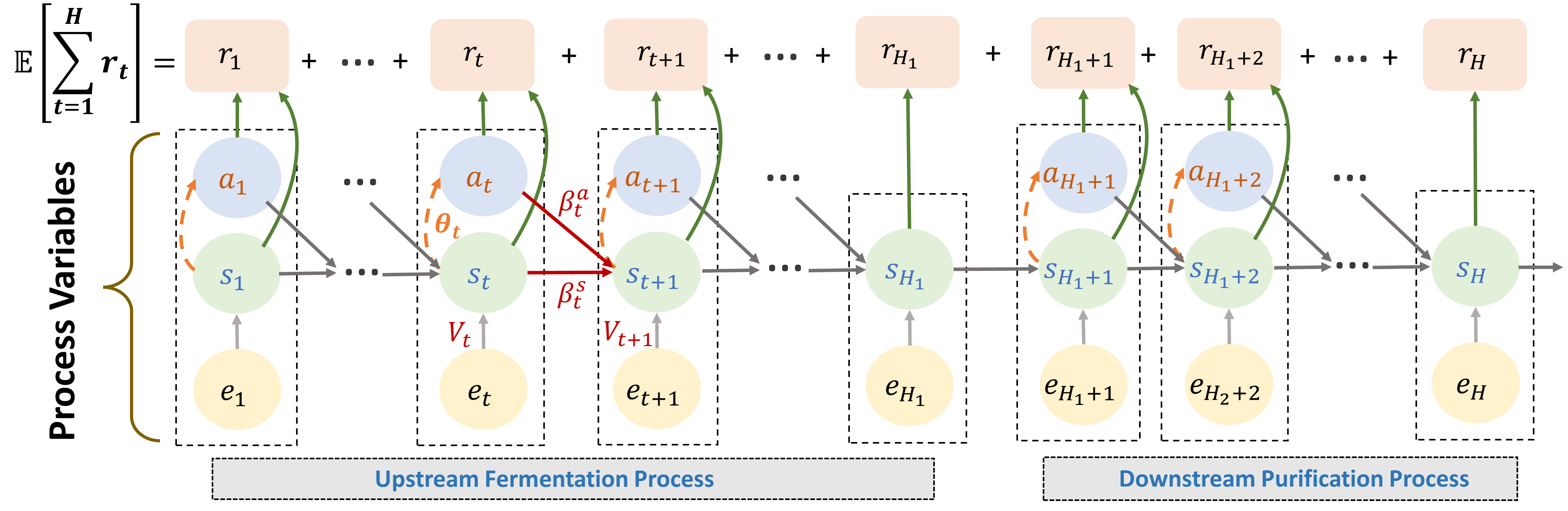
Figure 1: An illustration of a policy augmented Bayesian network (PABN) with arrows representing interactions.

With the introduction of policies and rewards, we create a policy augmented Bayesian network (PABN), as shown in Figure 1. The edges connecting nodes at time $t$ to nodes at time $t+1$ represent the process dynamics discussed in Section 3.1. The augmentation consists of additional edges 1) connecting state to action at the same time stage, representing the causal effect of the policy; and 2) connecting action and state to the immediate reward $r_{t}(\boldsymbol{s}_{t},\boldsymbol{a}_{t})$. To our knowledge, PABNs are a new modeling concept. Structurally, they have certain similarities to neural networks, in that we are choosing parameters to optimize outputs of the network, but a major difference is that state/action interactions are modeled explicitly at each step. PABNs support interpretable predictions of the effects of inputs at different times and their propagation through the bioprocess mechanism pathways.

3.3 Structural Properties for Predictive Analysis and Policy Optimization

Here we present two important computational results which will be used later to facilitate predictive analysis and policy optimization. The first result relates state $\boldsymbol{s}_{t+1}$ at any time $t+1$ to an earlier value $\boldsymbol{s}_{h}$ with $t\geq h$ connected through mechanism pathways as shown in Figure 1. There may be multiple paths connecting a given pair of nodes. For example, $\boldsymbol{s}_{t}$ is connected to $\boldsymbol{s}_{t+1}$ directly through the coefficient $\boldsymbol{\beta}^{s}_{t}$, but also through the action $\boldsymbol{a}_{t}$ via the coefficients $\boldsymbol{\beta}^{a}_{t}\boldsymbol{\vartheta}_{t}$. Thus, $\boldsymbol{s}_{t+1}$ depends on $\boldsymbol{s}_{h}$ through all possible pathways connecting the two. The nature of these dependencies is characterized in Proposition 1, whose detailed derivation is given in Appendix F.1.

Proposition 1

For any given decision epoch $t$ and starting state $\boldsymbol{s}_{h}$ with $h\in\{1,2,\ldots,t\}$, we have

$$\boldsymbol{s}_{t+1}=\boldsymbol{\mu}_{t+1}^{s}+\mathbf{R}_{h,t}(\boldsymbol{s}_{h}-\boldsymbol{\mu}^{s}_{h})+\left[\sum_{i=h}^{t}\mathbf{R}_{i,t}V_{i}\boldsymbol{z}_{i}+V_{t+1}\boldsymbol{z}_{t+1}\right],$$

where $V_{i}$ and $\boldsymbol{z}_{i}$ are as in (1), and $\mathbf{R}_{i,t}=\prod_{j=i}^{t}\left[\left(\boldsymbol{\beta}_{j}^{s}\right)^{\top}+\left(\boldsymbol{\beta}_{j}^{a}\right)^{\top}\boldsymbol{\vartheta}_{j}^{\top}\right]$ represents the product of pathway coefficients from time step $i$ to $t$.

Using Proposition 1, we can derive an explicit expression for the objective value $J\left(\pi_{\boldsymbol{\theta}};\boldsymbol{w}\right)$ of the linear policy $\pi_{\boldsymbol{\theta}}$, as well as the mean and variance of the state vector $\boldsymbol{s}_{t+1}$ under such a policy. Again, the derivation can be found in Appendix F.2. From this result, we can see the objective function is highly non-convex in the policy parameters $\boldsymbol{\theta}$.

Proposition 2

Fix a model specified by parameters $\boldsymbol{w}=(\boldsymbol{\mu}^{s},\boldsymbol{\mu}^{a},\boldsymbol{\beta},\boldsymbol{\sigma},\boldsymbol{v})$, a parametric linear policy $\pi_{\boldsymbol{\theta}}$, and an initial state vector $\boldsymbol{s}_{1}$. Then:

1. The mean and variance of $\boldsymbol{s}_{t+1}$ are given by

   $${\mathbb{E}}[\boldsymbol{s}_{t+1}] = \boldsymbol{\mu}_{t+1}^{s}+\mathbf{R}_{h,t}({\mathbb{E}}[\boldsymbol{s}_{h}]-\boldsymbol{\mu}^{s}_{h})=\boldsymbol{\mu}_{t+1}^{s}+\mathbf{R}_{1,t}(\boldsymbol{s}_{1}-\boldsymbol{\mu}^{s}_{1})~{}~{}\mbox{ for }h\in\{1,2,\ldots,t\}$$

   $$\mbox{Var}[\boldsymbol{s}_{t+1}] = \sum_{h=1}^{t}\mathbf{R}_{h,t}V_{h}^{2}\mathbf{R}_{h,t}^{\top}+V_{t+1}^{2}.$$

2. Under the linear reward structure of (2),

   $$J\left(\pi_{\boldsymbol{\theta}};\boldsymbol{w}\right)=\begin{cases}\sum^{H}_{t=1}\left\{m_{t}+\boldsymbol{b}_{t}^{\top}\boldsymbol{\mu}^{a}_{t}+\boldsymbol{c}_{t}^{\top}\boldsymbol{\mu}_{t}^{s}+(\boldsymbol{b}_{t}^{\top}\boldsymbol{\vartheta}_{t}^{\top}+\boldsymbol{c}_{t}^{\top})\mathbf{R}_{1,t}(\boldsymbol{s}_{1}-\boldsymbol{\mu}_{1}^{s})\right\}&\boldsymbol{w}\in\mathcal{W},\\ Hm_{c}&\boldsymbol{w}\notin\mathcal{W}.\end{cases}$$ (7)

3.4 Predictive Analysis Using the Shapley Value

Suppose that the model parameters $\boldsymbol{w}$ are given. We are interested in quantifying the contribution of each input, at any time $h$, to the expected future trajectory $\mbox{E}[\boldsymbol{s}_{t+1}|\boldsymbol{s}_{h},\boldsymbol{a}_{h}]$ with $t\geq h$. Specifically, let $\mathcal{O}_{h}=\{s^{k}_{h}\}_{k=1}^{n}\cup\{a^{k}_{h}\}_{k=1}^{m}$ denote the set of state and action inputs. The predicted contribution of any input ${o_{h}}\in\mathcal{O}_{h}$ is measured by the Shapley value

$$\mbox{Sh}\left(\boldsymbol{s}_{t+1}|{o_{h}};\boldsymbol{w}\right)=\sum_{\mathcal{U}\subset\mathcal{O}_{h}/\{{o_{h}}\}}\dfrac{(|\mathcal{O}_{h}|-|\mathcal{U}|-1)!|\mathcal{U}|!}{|\mathcal{O}_{h}|!}\left[g(\mathcal{U}\cup\left\{{o_{h}}\right\})-g(\mathcal{U})\right],$$

where $g(\cdot)={\mathbb{E}}[\boldsymbol{s}_{t+1}|\cdot;\boldsymbol{w}]$ represents the expected future trajectory based on the DBN model, and $|\mathcal{U}|$ is the cardinality of $\mathcal{U}\subset\mathcal{O}_{h}/\left\{o_{h}\right\}$. By definition, we have

$$f(\mathcal{O}_{h})={\mathbb{E}}[\boldsymbol{s}_{t+1}|\boldsymbol{s}_{h},\boldsymbol{a}_{h};\boldsymbol{w}]=\sum_{{o_{h}}\in\mathcal{O}_{h}}\mbox{Sh}\left(\boldsymbol{s}_{t+1}|{o_{h}};\boldsymbol{w}\right),$$

that is, the predicted mean is the sum of all the contributions. Then, we can use $\bar{\mbox{Sh}}\left(\boldsymbol{s}_{t+1}|{o_{h}}\right)=\int\mbox{Sh}(\boldsymbol{s}_{t+1}|{o_{h}};\boldsymbol{w})p(\boldsymbol{w}|\mathcal{D})d\boldsymbol{w}$ to assess the expected contribution of ${o_{h}}$ over the posterior distribution. Theorem 1 calculates the Shapley value (conditional on $\boldsymbol{w}$) in closed form for arbitrary $h$ and $t$; see the derivation in Appendix F.3. In this way, we can quantify how the influence of an input at time $h$ propagates far into the future.

Theorem 1

For any input $s^{k}_{h}$ and $a^{k}_{h}$, the Shapley value contribution is given by

$$\mbox{Sh}\left(\boldsymbol{s}_{t+1}|s_{h}^{k};\boldsymbol{w}\right) = \mathbf{R}_{h+1,t}\left(\boldsymbol{\beta}_{h}^{s}\right)^{{\top}}(s^{k}_{h}-\mu^{k}_{h})\mathrm{1}_{k}$$

$$\mbox{Sh}\left(\boldsymbol{s}_{t+1}|a_{h}^{k};\boldsymbol{w}\right) = \mathbf{R}_{h+1,t}\left(\boldsymbol{\beta}_{h}^{a}\right)^{\top}(a^{k}_{h}-\lambda^{k}_{h})\mathrm{1}_{k},$$

where $\mathrm{1}_{k}$ is the standard basis column vector whose components are all zero except the $k$th one equal to 1.

Though the Shapley values are derived for individual state and action inputs, the predictions used to calculate them are influenced by the control policy. Thus, the policy is indirectly reflected in the estimated contributions of various $o_{h}$. A more direct interpretation of the policy can be obtained by treating their policy parameters as action inputs and calculating their Shapley values. This falls outside the scope of the present paper, but is a subject for future work.

4 Policy Optimization with Projected Stochastic Gradients

In this section, we propose a policy optimization method to solve (4) with $\mathcal{P}$ restricted to the class of parametric linear policies introduced in (6). Essentially, we use gradient ascent to optimize $\mathcal{J}$ over the space of parametric linear policies, but there are some nuances in the analysis due to the fact that the space of policies is constrained to the set $\mathbb{C}$. Section 4.1 discusses the computation of the policy gradient, while Section 4.2 states the overall optimization framework in which the gradient computation is used.

4.1 Gradient Estimation and Computation

For notational convenience, we represent the parametric linear policy $\pi_{\boldsymbol{\theta}}$ by the parameter vector $\boldsymbol{\theta}$, and write $J,\mathcal{J}$ in (3) and (4) as functions of $\boldsymbol{\theta}$. We first establish the differentiability of the objective function $\mathcal{J}$, which will allow us to use gradient ascent to optimize the parameters. In the following, we understand $\boldsymbol{\theta}$ as a vector, i.e., $\boldsymbol{\theta}=\left(\text{vec}\left(\boldsymbol{\vartheta}_{1}\right),...,\text{vec}\left(\boldsymbol{\vartheta}_{H-1}\right)\right)^{\top}$, where $\text{vec}\left(\cdot\right)$ denotes a linear transformation converting an $n\times m$ matrix into a column vector. For notation simplification, we write the policy gradient $\nabla_{\boldsymbol{\theta}}\mathcal{J}\left(\boldsymbol{\theta}\right)$ as $\nabla\mathcal{J}\left(\boldsymbol{\theta}\right)$ in the following presentation.

Lemma 1

The objective function $\mathcal{J}$ is differentiable and its gradient satisfies

$$\nabla\mathcal{J}\left(\boldsymbol{\theta}\right)=\mathbb{E}_{\boldsymbol{w}\sim p\left(\boldsymbol{w}|\mathcal{D}\right)}\left[\nabla_{\boldsymbol{\theta}}J\left(\boldsymbol{\theta};\boldsymbol{w}\right)\right].$$ (8)

Furthermore, $\nabla\mathcal{J}$ is L-smooth over the closed convex set $\mathbb{C}$, that is,

$$\|\nabla\mathcal{J}(\boldsymbol{x})-\nabla\mathcal{J}(\boldsymbol{y})\|\leq L\lVert\boldsymbol{x}-\boldsymbol{y}\rVert,\qquad\boldsymbol{x},\boldsymbol{y}\in\mathbb{C}.$$

Equation (8) justifies the interchange of derivative and expectation, allowing us to focus on computing the gradient $\nabla_{\boldsymbol{\theta}}J\left(\boldsymbol{\theta};\boldsymbol{w}\right)$. The outer expectation over the posterior distribution of $\boldsymbol{w}$ can be estimated using sample average approximation (SAA) method: we use Gibbs sampling, as discussed in Section 3.1, to generate posterior samples $\left\{\boldsymbol{w}^{(b)}\right\}^{B}_{b=1}$ from the distribution $p\left(\boldsymbol{w}|\mathcal{D}\right)$, and calculate

$$\nabla\widehat{\mathcal{J}}(\boldsymbol{\theta})=\frac{1}{B}\sum^{B}_{b=1}\nabla_{\boldsymbol{\theta}}{J}\left(\boldsymbol{\theta};\boldsymbol{w}^{(b)}\right).$$ (9)

In the following discussion, we consider a fixed $h\in\left\{1,...,H-1\right\}$ as well as a fixed model $\boldsymbol{w}\in\mathcal{W}$. Recalling (3), we write

$$\nabla_{\boldsymbol{\vartheta}_{h}}{J}(\boldsymbol{\theta};\boldsymbol{w})=\sum^{H}_{t=1}\nabla_{\boldsymbol{\vartheta}_{h}}{\mathbb{E}}_{\boldsymbol{\tau}}\left[\left.r_{t}(\boldsymbol{s}_{t},\boldsymbol{a}_{t})\right|\boldsymbol{\pi}_{\boldsymbol{\theta}},\boldsymbol{s}_{1},\boldsymbol{{w}}\right].$$

By plugging in the reward and policy functions in (2) and (6), the expected reward becomes,

$${\mathbb{E}}_{\boldsymbol{\tau}}\left[\left.\sum_{t=1}^{H}r_{t}(\boldsymbol{s}_{t},\boldsymbol{a}_{t})\right|\boldsymbol{\pi}_{\theta},\boldsymbol{s}_{1},\boldsymbol{{w}}\right]=m_{t}+\boldsymbol{c}_{t}^{\top}{\mathbb{E}}[\boldsymbol{s}_{t}|\boldsymbol{\pi}_{\boldsymbol{\theta}},\boldsymbol{s}_{1},\boldsymbol{w}]+\boldsymbol{b}_{t}^{\top}\left(\boldsymbol{\mu}_{t}^{a}+\boldsymbol{\vartheta}_{t}^{\top}({\mathbb{E}}[\boldsymbol{s}_{t}|\boldsymbol{\pi}_{\boldsymbol{\theta}},\boldsymbol{s}_{1},\boldsymbol{w}]-\boldsymbol{\mu}_{t}^{s})\right).$$

Similarly, for $\boldsymbol{w}\notin\mathcal{W}$, we have $\mathbb{E}_{\boldsymbol{\tau}}\left[\left.\sum_{t=1}^{H}r_{t}(\boldsymbol{s}_{t},\boldsymbol{a}_{t})\right|\boldsymbol{\pi}_{\boldsymbol{\theta}},\boldsymbol{s}_{1},\boldsymbol{{w}}\right]=Hm_{c}$.

Let $\bar{\boldsymbol{s}}_{t}={\mathbb{E}}[\boldsymbol{s}_{t}|\boldsymbol{\pi}_{\boldsymbol{\theta}},\boldsymbol{s}_{1},\boldsymbol{w}]$. Using Propositions 1-2 and the functional forms of the reward and policy functions, we obtain an expression

$$\bar{r}_{t}(\boldsymbol{\theta};\boldsymbol{w})\equiv{\mathbb{E}}_{\boldsymbol{\tau}}\left[\left.r_{t}(\boldsymbol{s}_{t},\boldsymbol{a}_{t})\right|\boldsymbol{\pi}_{\boldsymbol{\theta}},\boldsymbol{s}_{1},\boldsymbol{{w}}\right]=m_{t}+\boldsymbol{c}_{t}^{\top}\bar{\boldsymbol{s}}_{t}+\boldsymbol{b}_{t}^{\top}(\boldsymbol{\mu}_{t}^{a}+\boldsymbol{\vartheta}_{t}^{\top}(\bar{\boldsymbol{s}}_{t}-\boldsymbol{\mu}_{t}^{s}))$$ (10)

for the expected reward at time $t$. This expression is equivalent to the one obtained in Proposition 2, but functionally it serves a different purpose: instead of expanding out all the pathways leading from time $1$ to time $t$, we instead represent them by $\bar{\boldsymbol{s}}_{t}$. We can also write a partial expansion of the pathways starting at some earlier time $h\leq t$. Such representations are crucial in policy optimization, where we need to evaluate partial derivatives of $\bar{r}_{t}$ with respect to $\boldsymbol{\vartheta}_{h}$ for just such an earlier time $h$. Thus, (10) leads into the following computational result; the proof is given in Appendix F.4.

Theorem 2 (Nested Backpropagation)

Let $\mathbf{R}_{h,t}$ be as in Proposition 1, with $\mathbf{R}_{t,t-1}=\mathbb{I}_{n\times n}$. Fix a model $\boldsymbol{w}$ and policy parameter vector $\boldsymbol{\theta}$. For any $h\leq t$, we have

$$\frac{\partial\bar{r}_{t}(\boldsymbol{\theta};\boldsymbol{w})}{\partial\boldsymbol{\vartheta}_{h}}=\begin{cases}(\boldsymbol{c}_{t}+\boldsymbol{\vartheta}_{t}\boldsymbol{b}_{t})(\bar{\boldsymbol{s}}_{h}-\boldsymbol{\mu}_{h}^{s})^{\top}\boldsymbol{\delta}_{h}^{t}&\text{if $h<t$}\\ (\bar{\boldsymbol{s}}_{h}-\boldsymbol{\mu}_{h}^{s})\boldsymbol{b}_{t}^{\top},&\text{if $h=t$}\end{cases}$$ (11)

where $\boldsymbol{\delta}_{h}^{t}=\mathbf{R}_{h+1,t-1}\left(\boldsymbol{\beta}_{h}^{a}\right)^{\top}$.

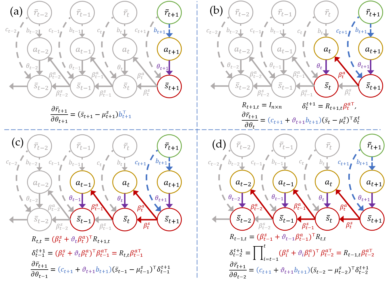
Figure 2: Illustration showing nested backpropagation computations, highlighting the pathways involved in each policy gradient calculation.

Theorem 2 gives us a computationally efficient way to update the gradient of $J\left(\boldsymbol{\theta};\boldsymbol{w}\right)$ which we call “nested backpropagation” to highlight both similarities and differences with the classic backpropagation algorithm used in the calibration of neural networks (Goh 1995). Each reward can be backpropagated to any policy parameter (say, $\boldsymbol{\vartheta}_{h}$) through the network or knowledge graph as shown in Figure 2. The term “backpropagation” refers to the fact that the calculation of gradients proceeds backward through the network, from time $t$ to time $h$. This structure is shared by neural networks. The key distinction, however, is that in our problem we must compute the gradient of $\bar{r}_{t}$ for every time period $t$, whereas in classic neural networks there is a single output function calculated at the final (terminal) node. Thus, there may be overlapping pathways between two such gradients, creating opportunities to save and reuse gradient computations. Specifically, the computation of $\frac{\partial\bar{r}_{t}}{\partial\boldsymbol{\theta}_{h}}$ can reuse the propagation pathways $\mathbf{R}_{h+1,t-1}$ through applying the equation

$$\mathbf{R}_{h,t-1}=(\boldsymbol{\beta}^{s}_{h}+\boldsymbol{\vartheta}_{h}\boldsymbol{\beta}_{h}^{a})^{\top}\mathbf{R}_{h+1,t-1}.$$

Figure 2 illustrates these reused computations through the examples (a) $\frac{\partial\bar{r}_{t+1}}{\partial\boldsymbol{\vartheta}_{t+1}}$, (b) $\frac{\partial\bar{r}_{t+1}}{\partial\boldsymbol{\vartheta}_{t}}$, (c) $\frac{\partial\bar{r}_{t+1}}{\partial\boldsymbol{\vartheta}_{t-1}}$ and (d) $\frac{\partial\bar{r}_{t+1}}{\partial\boldsymbol{\vartheta}_{t-2}}$. In Figure 2(a), the gradient $\frac{\partial\bar{r}_{t+1}}{\partial\boldsymbol{\vartheta}_{t+1}}$ is computed using only the nodes $r_{t+1}$, $\boldsymbol{a}_{t+1}$ and $\boldsymbol{s}_{t+1}$. In Figure 2(b), the gradient $\frac{\partial\bar{r}_{t+1}}{\partial\boldsymbol{\theta}_{t}}$ propagates the reward signal $\bar{r}_{t+1}$ back to $\boldsymbol{\vartheta}_{t}$, and the computation now uses information from the nodes $r_{t+1}$, $\boldsymbol{a}_{t+1}$, $\boldsymbol{s}_{t+1}$, $\boldsymbol{a}_{t}$ and $\boldsymbol{s}_{t}$ and associated edges. In Figure 2(d), we reuse the pathway $\mathbf{R}_{t,t}=(\boldsymbol{\beta}^{s}_{t}+\boldsymbol{\vartheta}_{t}\boldsymbol{\beta}_{t}^{a})^{\top}\mathbf{R}_{t+1,t}$ from Figure 2(c) to compute $\mathbf{R}_{t-1,t}=(\boldsymbol{\beta}^{s}_{t-1}+\boldsymbol{\vartheta}_{t-1}\boldsymbol{\beta}_{t-1}^{a})^{\top}\mathbf{R}_{t,t}$.

The formal statement of the nested backpropagation procedure is given in Algorithm 1. In Step (1), we first pass through the network to efficiently precompute the propagation pathways $\mathbf{R}_{h,t}$ through reuse, and store $\boldsymbol{\delta}_{h}^{t}$ that will be used multiple times to compute the gradients $\frac{\partial\bar{r}_{t}}{\partial\boldsymbol{\vartheta}_{h}}$ for $t=1,2,\ldots,H$ and $h=t-1,t-2,\ldots,1$ in Step (2). Proposition 3 proves that this approach reduces the cost of computing $\nabla_{\boldsymbol{\theta}}J\left(\boldsymbol{\theta};\boldsymbol{w}\right)$ by a factor of $\mathcal{O}\left(H\right)$ compared to a brute-force approach that does not reuse pathways. As will be shown in our computational study in Section 6.3, the time savings can be quite significant. The proof of Proposition 3 can be found in Appendix F.5.

Input: DBN coefficients $\boldsymbol{w}$, policy parameters $\boldsymbol{\vartheta}_{t}$, reward function $r_{t}(\bar{\boldsymbol{s}}_{t},\boldsymbol{a}_{t})=m_{t}+\boldsymbol{c}_{t}\bar{\boldsymbol{s}}_{t}+\boldsymbol{b}_{t}\boldsymbol{a}_{t}$ for all $t$;

1. Compute $\mathbf{R}_{h,t}$ and $\boldsymbol{\delta}^{t}_{h}$ with $t=1,2,\ldots,H$ and $h=1,2,\ldots,t$ as follows:

for $t=1,2,\ldots,H$ do

       Set $\mathbf{R}_{t+1,t}=I_{n\times n}$;

       for $h=t,t-1,\ldots,1$ do

             (a) $\boldsymbol{\delta}_{h}^{t}=\mathbf{R}_{h+1,t}\boldsymbol{\beta}^{a\top}_{h}$;

             (b) $\mathbf{R}_{h,t}=(\boldsymbol{\beta}_{h}^{s}+\boldsymbol{\vartheta}_{h}\boldsymbol{\beta}_{h}^{a})^{\top}\mathbf{R}_{h+1,t}$;

            

       end for

      

end for

2. Compute policy gradients $\frac{\partial\bar{r}_{t}}{\partial\boldsymbol{\vartheta}_{h}}$ for $t=1,2,\ldots,H$ as follows:

$\frac{\partial\bar{r}_{1}}{\partial\boldsymbol{\vartheta}_{1}}=(\bar{\boldsymbol{s}}_{1}-\boldsymbol{\mu}_{1}^{s})\boldsymbol{b}_{1}^{\top}$;

for $t=2,3,\ldots,H$ do

       $\frac{\partial\bar{r}_{t}}{\partial\boldsymbol{\vartheta}_{t}}=(\bar{\boldsymbol{s}}_{t}-\boldsymbol{\mu}_{t}^{s})\boldsymbol{b}_{t}^{\top}$;

       for $h=t-1,t-2,\ldots,1$ do

             $\frac{\partial\bar{r}_{t}}{\partial\boldsymbol{\vartheta}_{h}}=(\boldsymbol{c}_{t}+\boldsymbol{\vartheta}_{t}\boldsymbol{b}_{t}))(\bar{\boldsymbol{s}}_{h}-\boldsymbol{\mu}_{h}^{s})^{\top}\boldsymbol{\delta}_{h}^{t}$;

            

       end for

      

end for

3. Compute the policy gradientof the cumulative reward:

$$\nabla_{\boldsymbol{\theta}}J(\boldsymbol{\theta};\boldsymbol{w})=\left(\mbox{vec}\left(\sum^{H}_{t=1}\nabla_{\boldsymbol{\vartheta}_{1}}\bar{r}_{t}(\boldsymbol{\theta};\boldsymbol{w})\right),\ldots,\mbox{vec}\left(\sum^{H}_{t=1}\nabla_{\boldsymbol{\vartheta}_{H-1}}\bar{r}_{t}(\boldsymbol{\theta};\boldsymbol{w})\right)\right)^{\top}.$$

Algorithm 1 Nested backpropagation procedure for policy gradient computation.

Proposition 3

Fix a model $\boldsymbol{w}$ and policy parameters $\boldsymbol{\theta}$. The cost to compute $\nabla_{\boldsymbol{\theta}}J(\boldsymbol{\theta};\boldsymbol{w})$ is $\mathcal{O}\left(H^{2}n^{2}m\right)$ for nested backpropagation (Algorithm 1) and $\mathcal{O}\left(H^{3}n^{2}m\right)$ for brute force.

4.2 Policy Optimization Algorithm

Recall that the gradient of $\mathcal{J}$ is estimated using SAA in (9), with ${J}\left(\boldsymbol{\theta};\boldsymbol{w}^{(b)}\right)$ computed using Algorithm 1. We can now search for the optimal $\boldsymbol{\theta}$ using a recursive gradient ascent update. Given $\boldsymbol{\theta}_{k}$, we compute

$$\boldsymbol{\theta}_{k+1}=\Pi_{\mathbb{C}}\left(\boldsymbol{\theta}_{k}+\eta_{k}\nabla\widehat{\mathcal{J}}\left(\boldsymbol{\theta}_{k}\right)\right),$$ (12)

where $\eta_{k}$ is a suitable stepsize, $\mathbb{C}$ is a closed convex feasible region as discussed in Section 3.2, and $\Pi_{\mathbb{C}}$ is a projection onto $\mathbb{C}$. The projection of a point $\boldsymbol{y}$ onto ${\mathbb{C}}$ is defined as $\Pi_{\mathbb{C}}(\boldsymbol{y})=\mathop{\rm arg\,min}_{\boldsymbol{x}\in{\mathbb{C}}}\frac{1}{2}\lVert\boldsymbol{x}-\boldsymbol{y}\rVert^{2}.$ We summarize some previously established properties of the projection, which will be needed for our convergence analysis later; the proofs are given in Section 2.2 of Jain and Kar (2017), and thus are omitted here. Throughout the paper, we use the usual Euclidean norm and inner product.

Proposition 4

For any set ${\mathbb{C}}\subset\mathbb{R}^{p}$, the following inequalities hold:

1. If $\boldsymbol{y}\in{\mathbb{C}}$, then $\Pi_{\mathbb{C}}(\boldsymbol{y})=\boldsymbol{y}$.

2. For any $\boldsymbol{y}\in\mathbb{R}^{p}$ and $\boldsymbol{x}\in{\mathbb{C}}$, $\|\Pi_{\mathbb{C}}(\boldsymbol{y})-\boldsymbol{y}\|\leq\|\boldsymbol{x}-\boldsymbol{y}\|$.

3. If $\mathbb{C}$ is convex, $\Pi_{\mathbb{C}}$ is non-expansive. That is, for any $\boldsymbol{x},\boldsymbol{y}\in\mathbb{R}^{p}$,

   $$\|\Pi_{\mathbb{C}}(\boldsymbol{x})-\Pi_{\mathbb{C}}(\boldsymbol{y})\|^{2}\leq\langle\Pi_{\mathbb{C}}(\boldsymbol{x})-\Pi_{\mathbb{C}}(\boldsymbol{y}),\boldsymbol{x}-\boldsymbol{y}\rangle\leq\|\boldsymbol{x}-\boldsymbol{y}\|^{2}.$$

4. For any convex set ${\mathbb{C}}\in\mathbb{R}^{p}$, $\boldsymbol{y}\in\mathbb{R}^{p}$ and $\boldsymbol{x}\in{\mathbb{C}}$, we have $\langle\boldsymbol{x}-\Pi_{\mathbb{C}}(\boldsymbol{y}),\boldsymbol{y}-\Pi_{\mathbb{C}}(\boldsymbol{y})\rangle\leq 0.$

It is sometimes convenient to rewrite (12) as

$$\boldsymbol{\theta}_{k+1}=\boldsymbol{\theta}_{k}+\eta_{k}\widehat{g}_{k}\left(\boldsymbol{\theta}_{k}\right)~{}~{}\mbox{ with }~{}~{}\widehat{g}_{k}\left(\boldsymbol{\theta}\right)=\frac{1}{\eta_{k}}\left(\Pi_{\mathbb{C}}\left(\boldsymbol{\theta}+\eta_{k}\nabla\widehat{\mathcal{J}}\left(\boldsymbol{\theta}\right)\right)-\boldsymbol{\theta}\right)$$ (13)

where $\widehat{g}_{k}\left(\boldsymbol{\theta}\right)$ can be viewed as a generalized gradient estimator. This representation is identical to (12), except that (13) resembles an unconstrained gradient ascent update.

The complete statement of the policy optimization procedure, which we call DBN-RL (“DBN-assisted reinforcement learning”), is given in Algorithm 2. In each iteration, we generate $B$ model parameters, $\left\{\boldsymbol{w}^{(b)}\right\}^{B}_{b=1}$, by sampling from the posterior distribution $p\left(\boldsymbol{w}|\mathcal{D}\right)$, then use nested backpropagation to calculate gradients for each individual model. We then average over the models and apply (13) to update the policy parameters. It is worth noting that the only randomness in this stochastic gradient method comes from the use of SAA to approximate the expectation in (5) with an average over $B$ posterior samples in (9). The computational results of Theorem 2 and Algorithm 1 allow us to explicitly compute $\nabla_{\boldsymbol{\theta}}{J}\left(\boldsymbol{\theta};\boldsymbol{w}^{(b)}\right)$ for $b=1,2,\ldots,B$.

Input: the maximum number of episodes $K$; the convex constraint set $\mathbb{C}$; initial parameter $\boldsymbol{\theta}_{0}$ for linear policy $\boldsymbol{\pi}_{\boldsymbol{\theta}_{0}}(\boldsymbol{s})$, $\forall\boldsymbol{s}\in\mathcal{S},\boldsymbol{\theta}\in\mathbb{C}$; posterior distribution $p(\boldsymbol{w}|\mathcal{D})$ for process knowledge graph model;

for $k=1,2,\ldots,K$ do

       1. Generate $B$ posterior samples of process model parameters $\boldsymbol{w}_{k}^{(b)}\sim p(\boldsymbol{w}|\mathcal{D})$ with $b=1,2,\ldots,B$;

       for $b=1,2,\ldots,B$ do

             if $\boldsymbol{w}_{k}^{(b)}\in\Omega$ then

                   Calculate the policy gradient $\nabla_{\boldsymbol{\theta}}J(\boldsymbol{\theta}_{k};\boldsymbol{w}_{k}^{(b)})$ by using Algorithm 1; 

            else

                   $\nabla_{\boldsymbol{\theta}}J(\boldsymbol{\theta}_{k};\boldsymbol{w}_{k}^{(b)})=0$; 

             end if

            

       end for

       3. Calculate $\nabla\widehat{\mathcal{J}}(\boldsymbol{\pi}_{\boldsymbol{\theta}})=\frac{1}{B}\sum^{B}_{b=1}\nabla_{\boldsymbol{\theta}}J\left(\boldsymbol{\pi}_{\boldsymbol{\theta}};\boldsymbol{w}_{k}^{(b)}\right)$;

        4. Obtain the gradient mapping $\widehat{g}_{c}(\boldsymbol{\theta}_{k})=\frac{1}{\eta_{k}}(\tilde{\boldsymbol{\theta}}_{k}-\boldsymbol{\theta}_{k})$, where $\tilde{\boldsymbol{\theta}}_{k}=\Pi_{C}\left(\boldsymbol{\theta}_{k}+\eta_{k}\nabla\widehat{\mathcal{J}}(\boldsymbol{\theta}_{k})\right)$;

        5. Update the policy parameters $\boldsymbol{\theta}_{k+1}\leftarrow\boldsymbol{\theta}_{k}+\eta_{k}\widehat{g}_{c}(\boldsymbol{\theta}_{k})$.

end for

Algorithm 2 DBN-RL algorithm for policy optimization.

5 Convergence Analysis

Here we prove the convergence of DBN-RL to a local optimum of $\mathcal{J}$ and characterize the convergence rate. Recall from Proposition 2 that $\mathcal{J}$ is non-convex in $\boldsymbol{\theta}$. Consequently, only local convergence can be guaranteed, as is typical of stochastic gradient ascent methods.

There is a rich literature on the convergence analysis of this class of algorithms. However, the proofs often rely on very subtle nuances in model assumptions, e.g., on the level of noise or the smoothness of the objective function. The classical theory (see, e.g., Kushner and Yin 2003) has focused on almost sure convergence (e.g., of $\nabla\mathcal{J}\left(\boldsymbol{\theta}_{k}\right)$ to zero). The work by Bertsekas and Tsitsiklis (2000) gives some of the weakest assumptions for this type of convergence when the objective is non-convex. Nemirovski et al. (2009) pioneered a different style of analysis which derived convergence rates. This initial work required weakly convex objectives, but the non-convex setting was variously studied by Ghadimi and Lan (2013), Jain and Kar (2017), and Li and Orabona (2019). Our analysis belongs to this overall stream, but derives convergence rates in the presence of a projection operator, with weaker assumptions than past papers studying similar settings.

We first note that the specific objective function optimized by DBN-RL was shown to be $L$-smooth in Lemma 1. A direct consequence of this property (Lemma 1.2.3 of Nesterov 2003), used in our analysis, is that

$$|\mathcal{J}(\boldsymbol{y})-\mathcal{J}(\boldsymbol{x})-\langle\nabla\mathcal{J}(\boldsymbol{x}),\boldsymbol{y}-\boldsymbol{x}\rangle|\leq L\lVert\boldsymbol{x}-\boldsymbol{y}\rVert^{2}.$$ (14)

For notational simplicity, we use ${\mathbb{E}}$ to refer to the expectation over the posterior distribution $p\left(\boldsymbol{w}|\mathcal{D}\right)$, since this distribution is the only source of randomness in the algorithm. Also let

$$A_{k}=\left\{\boldsymbol{\theta}_{k}+\eta_{k}\nabla\widehat{\mathcal{J}}(\boldsymbol{\theta}_{k})\in\mathbb{C}\right\}$$ (15)

be the event that the updated gradient remains in the feasible region (i.e., we do not need to project it back onto $\mathbb{C}$) after the $k$-th episode.

Three additional assumptions are required for the convergence proof.

Assumption 1 (Boundary condition)

For any $\boldsymbol{\theta}\in\partial\mathbb{C}$ and model $\boldsymbol{w}\in\mathcal{W}$, there exists a constant $c_{0}>0$ such that, when the stepsize $\eta\leq c_{0}$, we have $\boldsymbol{\theta}+\eta\frac{\nabla_{\boldsymbol{\theta}}{J}(\boldsymbol{\theta};\boldsymbol{w})}{\|\nabla_{\boldsymbol{\theta}}{J}(\boldsymbol{\theta};\boldsymbol{w})\|}\in\mathbb{C}.$

Assumption 1 suggests that, at any point on the boundary of the feasible region, the gradient always points toward the interior of $\mathbb{C}$. For example, one might consider a situation where the feasible region is large enough to include all local maxima. This assumption is reasonable for biomanufacturing, because in such an application $\mathbb{C}$ should be defined based on FDA regulatory requirements; any batch outside the required region will induce a massive penalty.

Assumption 2 (Noise level)

For any $\boldsymbol{\theta}\in\mathbb{C}$, we have ${\mathbb{E}}[\|\nabla\widehat{\mathcal{J}}(\theta)-{\nabla\mathcal{J}}(\theta)\|^{4}]^{1/4}\leq\sigma$.

Classical stochastic approximation theory (Kushner and Yin 2003) assumes uniformly bounded variance, i.e., ${\mathbb{E}}\left[\|\nabla\widehat{\mathcal{J}}(\theta)-{\nabla\mathcal{J}}(\theta)\|^{2}\right]\leq\sigma^{2}$. This assumption is weaker than Assumption 2, but the results will also be weaker since the classical theory is primarily concerned with almost sure convergence only. If we compare against existing work on convergence rates, Assumption 2 is weaker than other widely used assumptions such as ${\mathbb{E}}[\exp{(\|\nabla\widehat{\mathcal{J}}(\theta)-{\nabla\mathcal{J}}(\theta)\|^{2}}/\sigma^{2})]\leq\exp{(1)}$, used in Nemirovski et al. (2009) and Li and Orabona (2019). For non-convex and strongly convex cases, one can also find other assumptions, such as boundedness $\|\nabla\widehat{\mathcal{J}}(\theta)-{\nabla\mathcal{J}}(\theta)\|^{2}\leq S$ of the stochastic gradient itself (Li and Orabona 2019), or boundedness ${\mathbb{E}}\left[\|\nabla\widehat{\mathcal{J}}(\theta)\|^{2}\right]\leq\sigma^{2}$ of the second moment of the gradient estimator (Shalev-Shwartz et al. 2011, Recht et al. 2011). Assumption 2 is weaker than all of these.

Assumption 3

The global maximum $\boldsymbol{\theta}^{\star}$ lies in the interior of $\mathbb{C}$, that is, $\boldsymbol{\theta}^{\star}\in\mathbb{C}\backslash\partial\mathbb{C}$ and $\mathcal{J}(\boldsymbol{\theta})\leq\mathcal{J}(\boldsymbol{\theta}^{\star})$ for any $\boldsymbol{\theta}\in\mathbb{C}$.

Assumption 3 guarantees that the feasible region is large enough to include the optimal solution, complementing Assumption 1, which ensures that the gradient points us back toward the interior if we are ever close to leaving the feasible region.

We can now proceed with the analysis; proofs of the main results and lemmas can be found in Appendix F.7-F.11. First, by applying Lemma 1 and Assumption 3, we can show that the true policy gradient $\nabla\mathcal{J}(\boldsymbol{\theta})$ is bounded on the feasible region.

Corollary 1

For any $\boldsymbol{x}\in\mathbb{C}$, we have $\|\nabla\mathcal{J}(\boldsymbol{x})\|\leq\max_{\boldsymbol{x}\in\mathbb{C}}\|\nabla\mathcal{J}(\boldsymbol{x})\|\leq G$, where $G=L\cdot\max_{\boldsymbol{y}\in\mathbb{C}}\|\boldsymbol{y}-\boldsymbol{\theta}^{\star}\|^{2}$.

Recalling the definition of $A_{k}$ in (15), we let $p\left(A_{k}\right)$ be the probability that the updated gradient after the $k$-th iteration remains in $\mathbb{C}$. We then show that, on almost every sample path, this will happen for all sufficiently large $k$.

Lemma 2

Let Assumptions 1-3 hold and suppose $\sum^{\infty}_{k=1}\eta_{k}^{2}<\infty$. Then,

$$\lim_{k\rightarrow\infty}p(A_{k})=\lim_{k\rightarrow\infty}P\left(\boldsymbol{\theta}_{k}+\eta_{k}\nabla\widehat{\mathcal{J}}(\boldsymbol{\theta}_{k})\in\mathbb{C}\right)=1.$$

The final convergence result connects $p\left(A_{k}\right)$ to the averaged expected norm $\frac{1}{K}\sum_{k=1}^{K}{\mathbb{E}}\left[\|\nabla\mathcal{J}(\boldsymbol{\theta}_{k})\|^{2}\right]$ of the true policy gradient.

Theorem 3

Let Assumptions 1-3 hold, and suppose that the stepsize satisfies $\sum^{\infty}_{k=1}\eta_{k}^{2}<\infty$. Then,

$$\frac{1}{K}\sum_{k=1}^{K}{\mathbb{E}}\left[\|\nabla\mathcal{J}(\boldsymbol{\theta}_{k})\|^{2}\right]\leq\frac{\frac{2}{\eta_{1}}\left(\mathcal{J}^{\star}-\mathcal{J}(\boldsymbol{\theta}_{1})\right)+2(G^{2}+G\sigma)\sum_{k=1}^{K}(1-p(A_{k}))^{1/2}+8L\sigma^{2}\sum_{k=1}^{K}\eta_{k}}{K}.$$

Thus, the convergence rate of our algorithm is connected to the behavior of $p\left(A_{k}\right)$. Combining Lemma 2 with Theorem 3, we have $\frac{1}{K}\sum_{k=1}^{K}{\mathbb{E}}\left[\|\nabla\mathcal{J}(\boldsymbol{\theta}_{k})\|^{2}\right]\rightarrow 0.$

6 Empirical Study

We present a case application of our approach to multi-phase fermentation of Yarrowia lipolytica, a process in which viable cells grow and produce the biological substance of interest. In Section 6.1, we develop a simulator based on real-world experimental data and domain knowledge of bioprocess mechanisms. In Section 6.2, we use this simulator to assess the performance of the proposed DBN-RL framework and compare it with a state-of-the art RL benchmark. Section 6.3 provides additional empirical evidence that there is value in accounting for model risk, especially when the stochastic uncertainty is high and the number of observations is low. In Section 6.4, we discuss the interpretability of the proposed framework. Finally, in Section 6.5, we present additional empirical results showing how the proposed framework can support integrated biomanufacturing process control.

6.1 Description of Application and Simulator

The simulator is constructed using existing domain knowledge of fermentation process kinetics, as well as 8 batches of real data from lab experiments. Domain knowledge is leveraged by fitting an ODE-based nonlinear kinetic model, with the addition of a Wiener process to represent intrinsic stochastic uncertainty; the details can be found in Appendix D. Then, to mimic “real-world data" collection, we generate the data $\mathcal{D}$ consisting of $R$ process observations (replications from the simulator).

We have a five-dimensional continuous state variable $\boldsymbol{s}=(X_{f},C,S,N,V)$, where $X_{f}$ represents lipid-free cell mass; $C$ measures citrate, the actual “product” to be harvested at the end of the bioprocess, generated by the cells’ metabolism; $S$ and $N$ are amounts of substrate (a type of oil) and nitrogen, both used for cell growth and production; and $V$ is the working volume of the entire batch. We also have one scalar continuous CPP action ${a}=F_{S}$, which represents the feed rate, or the amount of new substrate given to the working cells in one unit of time.

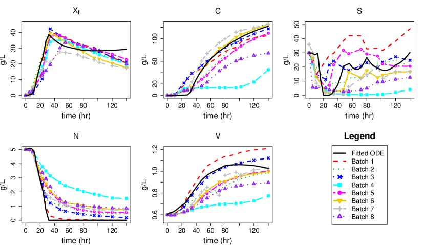
Figure 3: ODE trajectory (in black) and 8 batches of real lab experiment trajectories. Batches 4 and 8, which have low productivity, are two experiments with low oil feed.

Figure 3 illustrates the historical trajectories of each CQA from all 8 batches of process observations, as well as the trajectory obtained from the estimated kinetic model. One can see that there is a great deal of variation between real experiments; the given data are not sufficient to estimate intrinsic stochastic uncertainty because each experiment was conducted with very different decision parameters. Thus, we chose to set the inherent stochastic uncertainty of state $\boldsymbol{s}_{t}=(X_{ft},C_{t},S_{t},N_{t},V_{t})$ at time $t$ as

$$\sigma(s_{t})={\frac{1}{8\kappa}\sum_{i=1}^{8}s^{(i)}_{t}},$$ (16)

a multiple of the estimated mean over $8$ experiments. In our numerical study, we considered $\kappa\in\left\{10,25,\infty\right\}$, reflecting different levels of stochastic uncertainty which depend on both time and state. We use $\sigma(s_{t})$ as the variation parameter in the Wiener process, as described in Appendix D.

The initial state $\boldsymbol{s}_{1}$ was chosen randomly to account for raw material variation. Our process knowledge graph consists of 215 nodes and 770 edges with 36 time measurement steps (proceeding in increments of four hours, up to the harvest time of $140$ hours). There are $35$ transitions, $5$ CQA state nodes (one for each continuous dimension) and one CPP action node per time period, leading to a total of $985$ parameters to estimate using Gibbs sampling. The region $\mathcal{W}$ of valid model parameters was chosen to ensure that each parameter is bounded by a large constant $10^{10}$.

This simulator was then used to generate $R$ simulated trajectories. In each of these, we chose the feed rate action according to the $\epsilon$-greedy method (Sutton and Barto 2018), which balances exploration and exploitation:

$${a}_{t}=\begin{cases}a_{t}^{h}+\mathcal{N}(0,\bar{a}_{t}/10),&\text{with probability $0.7$},\\ \mbox{Unif}(0,\max_{t\in\mathcal{T}}\{\bar{a}_{t}\}),&\text{with probability $0.3$}.\end{cases}$$

Here, $\bar{{a}}_{t}$ denotes the maximum feed rate across our 8 real experiments at time $t$, and $a_{t}^{h}$ denotes the average feed rate across these experiments. In words, we randomly choose either the average feed rate from the real data (with some noise), or a uniformly distributed quantity between zero and the maximum feed rate.

The reward function at time $t$ was formulated by consultation with biomanufacturing experts, and is based on the citrate concentration $C_{t}$ and feed rate $a_{t}$ according to

$$r(\boldsymbol{s}_{t},{a}_{t})=\begin{cases}-15+1.29C_{t},&\text{if $t=H$},\\ -534.52{a}_{t},&\text{if $0\leq t<H$}.\end{cases}$$

This structure reflects the fact that, during the process, the operating cost is primarily driven by the substrate, and the product revenue is collected at the harvest time.

The linear policy (6) is non-stationary; since there are $35$ state transitions, five state nodes and one action node, the total number of policy parameters is $175$. Based on consultation with biomanufacturing experts, the feasible region $\mathbb{C}$ was chosen by constraining each individual parameter to an interval. The lower and upper bounds are the same for all parameters corresponding to a particular CQA (dimension of the state variable). For cell mass and citrate, we used the interval $[0,0.3]$ as the action (feed rate of substrate) always positively affects cell growth and citrate production. For substrate, we used the interval $[-0.1,0.1]$ because excessively high substrate concentration may have adverse effects. For nitrogen, we used the interval $[-0.1,0.02]$, and for volume, we used $[-0.7,0.5]$. Policy parameters can be negative because excessive nutrients can lead to stresses on living cells, which reduces productivity.

6.2 Performance Comparison

We compare DBN-RL against Deep Deterministic Policy Gradient (DDPG), a state-of-the-art model-free RL algorithm designed for continuous control (Lillicrap et al. 2016), as well as with a “human” policy inferred from the 8 real experiments (see Figure 3). Although we are not given an exact policy used by human experts (and it is unlikely that they follow any explicit policy in practice), their observed actions are based on their domain knowledge and so the inferred policy may be quite competitive in some situations.

DDPG attempts to learn the value of a policy and simultaneously improve it. The value of a policy is modeled using a deep network with a multi-layer feed-forward architecture which evaluates each state-action pair. Because the DDPG method was designed to find stationary policies, the time $t$ has to be added as an extra dimension into the state variable. The deep network contains a 7-dimensional state input layer followed by a dense layer with 64 neurons. The 64-dimensional dense layer is concatenated with an (1-dimensional) action input layer and then followed by a 8-dimensional dense layer; the output layer is 1-dimensional with a linear activation function. The policy improvement step uses another, two-layer neural network with the state input followed by an 8-dimensional intermediate layer and a 1-dimensional action output layer with a “tanh" activation function.

Table 1: Reward and final citrate titer of DBN-RL, DDPG and human policy (30 macro-replications).

Algorithms		DBN-RL				DDPG				Human
Sample Size	$\kappa$	Reward		Titer (g/L)		Reward		Titer (g/L)		Reward		Titer (g/L)
		Mean	SE	Mean	SE	Mean	SE	Mean	SE	Mean	SE	Mean	SE
$R=8$	10	103.44	2.50	101.15	1.11	-		-		113.47	4.26	102.12	3.88
	25	108.13	2.06	103.15	1.11	-		-		116.19	4.03	103.71	3.45
	$\infty$	114.96	1.73	105.93	0.94	-		-		118.76	3.56	104.86	3.10
$R=15$	10	119.75	1.60	110.62	0.84	17.65	11.53	39.16	8.27	-		-
	25	120.11	1.64	111.62	0.93	23.35	10.83	47.11	8.40	-		-
	$\infty$	121.35	1.75	111.98	0.90	20.65	10.24	49.04	7.12	-		-
$R=50$	10	126.94	2.15	115.29	1.19	24.65	9.00	50.33	6.41	-		-
	25	128.34	1.23	115.13	4.52	20.44	8.04	45.93	6.10	-		-
	$\infty$	131.97	0.47	116.05	0.41	21.65	7.18	49.33	5.45	-		-
$R=100$	10	128.90	1.25	115.89	0.60	31.36	10.98	45.21	8.24	-		-
	25	130.73	0.95	116.02	0.59	32.89	10.14	50.23	8.60	-		-
	$\infty$	131.92	0.73	116.35	0.45	35.89	9.88	51.81	7.85	-		-
$R=400$	10	130.40	0.57	116.45	0.38	37.23	9.12	50.43	8.28	-		-
	25	131.01	0.37	116.75	0.30	37.43	9.95	52.43	8.87	-		-
	$\infty$	133.04	0.12	118.12	0.14	39.77	9.23	55.16	9.29	-		-
$R=3000$	$\infty$	-		-		119.28	0.84	104.78	0.74	-		-

Table 1 reports the total expected reward, as well as the final citrate titer production (amount of product harvested at the end of $140$ hours) obtained by each policy. A total of 30 macroreplications was conducted. We see that, under the smallest sample size $R=8$, the human policy achieves the best performance, as might be expected from domain experts. However, with only a few additional samples from the simulator (i.e., $R=15$), DBN-RL can improve on the human policy, with additional improvement as $R$ increases.

The DDPG policy is much less efficient than DBN-RL, because it is entirely model-free and cannot benefit from domain knowledge of the structured interactions between CPPs and CQAs. For demonstration purposes, we report the performance of DDPG for a very large sample size of $R=3000$, simply to show that this policy is indeed able to do reasonably well when given enough data. However, even these numbers are not as good as what DBN-RL can achieve with just $R=15$ samples. In some runs, we observed that DDPG diverged during training, even after several thousand episodes. Similar convergence issues have been reported by Matheron et al. (2019). Moreover, in some cases DDPG converged to the boundaries of the action space rather than the true optimum, perhaps because the boundaries are local optima.

6.3 Model Risk and Computational Efficiency

We present additional empirical results demonstrating the benefits of directly building model risk into the DBN, as well as the computational savings obtained by using the proposed nested backpropagation procedure (Algorithm 1). First, we compare DBN-RL as stated in Algorithm 2 with another version of DBN-RL that ignores model risk. In this second version, the posterior samples $\boldsymbol{w}^{(b)}$ are replaced by a single point estimate (i.e., posterior mean) of the model parameters. The results in Table 2 show that we can obtain a better policy when we account for model risk, especially when the amount of data is small and stochastic uncertainty is high.

Table 2: Performance of DBN-RL with and without model risk ($\kappa=5,10$ and 30 macro-replications).

$\kappa$	Sample size	Metrics	DBN-RL with MR	DBN-RL ignoring MR	$p$-value
$10$	$R=8$	Reward	103.44 (2.50)	95.39 (2.19)	<0.001
		Titer (g/L)	101.15 (1.11)	96.64 (0.96)	<0.001
	$R=15$	Reward	119.75 (1.60)	118.35 (1.81)	0.56
		Titer (g/L)	118.35 (0.84)	109.12 (0.94)	<0.001
$5$	$R=8$	Reward	102.91 (2.45)	94.06 (2.53)	0.01
		Titer (g/L)	100.29 (1.25)	95.08 (1.46)	0.01
	$R=15$	Reward	118.92 (1.39)	114.74 (1.68)	0.06
		Titer (g/L)	115.29 (1.19)	105.99 (0.98)	<0.001

Next, we compare the computational cost of DBN-RL with and without nested backpropagation. When Algorithm 1 is not used, the policy gradient is computed using brute force. Table 3 reports mean computational time in minutes (averaged over 30 macro-replications) for different sample sizes $R$ and time horizons $H$. For reference, we also report the training time for the dynamic Bayesian network (i.e., the Bayesian inference calculations, which are unrelated to policy optimization). It is clear that the brute-force method scales very poorly with the process complexity $H$. In practice, $H$ tends to be much greater than the sample size $R$, meaning that nested backpropagation is much more scalable. When $R=15,100,400$ and $H=36$, the computation time (mean $\pm$ SE) of DDPG is $6.1\pm 0.4$, $13.1\pm 0.8$, and $48.2\pm 3.0$ minutes, which is comparable with the time taken by DBN-RL with NBP.

Table 3: Computational time (in minutes) of DBN-RL with and without nested backpropagation.

Horizon	$R=15$			$R=100$			$R=400$
	Training	NBP	Brute Force	Training	NBP	Brute Force	Training	NBP	Brute Force
$H=8$	1.1 (0.1)	0.8 (0.1)	5.9 (0.2)	3.9 (0.1)	0.8 (0.1)	5.6 (0.2)	14.9 (0.3)	0.8 (0.1)	6.1 (0.2)
$H=15$	2.4 (0.7)	2.1 (0.4)	27.4 (1.2)	8.7 (0.3)	2.4 (0.3)	26.9 (1.2)	31.5 (2.3)	2.0 (0.4)	28.1 (1.1)
$H=36$	4.1 (0.2)	9.1 (0.3)	302.3 (5.3)	17.9 (0.1)	9.7 (0.8)	312.3 (5.6)	59.7 (0.6)	10.1 (0.7)	310.5 (6.1)

6.4 Interpretability of DBN-RL

A well-known limitation of model-free reinforcement learning techniques (such as those based on deep neural networks) is their lack of interpretability. This can be a serious concern, because the average value of a single batch of bio-drug product is worth over $\$1$million. The proposed DBN-RL framework can overcome this limitation. First, the network structure provides an intuitive visualization of the quantitative associations between CPPs and CQAs. Second, the policy learned from DBN-RL behaves in a way that is understandable to human experts, as demonstrated by the following example.

We fix an initial state $\boldsymbol{s}_{1}=(0.05,0,30,5,0.6)$ and simulate the actions (feeding rates) taken over time by following the policies obtained from DBN-RL, DDPG, and human experts. For each time $t$, we then average the action $a_{t}$ and plot these averages over time to obtain a feeding profile for each type of policy. These profiles are shown in Figure 4. The policies learned by DBN-RL suggest starting out with low initial feeding rates, because the high initial substrate ($S_{1}=30$ g/L) is sufficient for biomass development (providing enough carbon sources for cell proliferation and early citrate formation). DBN-RL then ramps up feeding rapidly until the amount of substrate reaches approximately $10$ g/L, when the biomass growth rate is highest. After $24$ hours, DBN-RL begins to reduce the feeding rate, and generally continues doing so until the end of the process. This occurs because the life cycle of cells moves from the growth phase to the production phase at around $24$ hours, and less substrate is required to support production. Comparing with Figure 4(b), we find that the feeding profile of DBN-RL has a very similar curve to that of the human expert policy, and even peaks around the same time. On the other hand, DDPG does not supply enough substrate for biomass growth during the first $30$ hours, lowering the cell growth rate; it then attempts to compensate later on, but this is ineffective because of intensive inhibition from high substrate concentration.

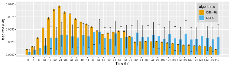
(a) Feeding profiles of DBN-RL and DDPG with 95% confidence intervals. (R$=400$)

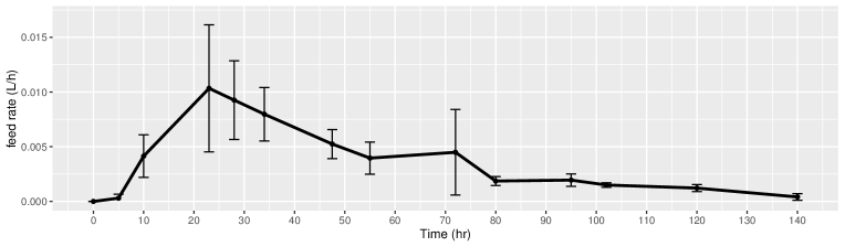
(b) Feeding profile from human experts: averaged trajectory with 95% confidence intervals.

Figure 4: Feeding profiles obtained from (a) RL algorithms and (b) human experts.

Next, we illustrate how the Shapley value analysis of Section 3.4 helps with interpretability. We consider two representative scenarios, namely batches 5 and 8 from Figure 3, with $R=15$ observations and stochastic uncertainty $\kappa=10$. At the current time $t=15$ (60 hr), we have $\mathcal{O}_{t}=\{X_{f,t},C_{t},S_{t},N_{t},V_{t},F_{St}\}$. We use the expected Shapley value $\bar{\mbox{Sh}}\left(C_{H}|x\right)$ to quantify the contribution of each input $x\in\mathcal{O}_{t}$ to the predicted expected citrate concentration at the end of the fermentation process.

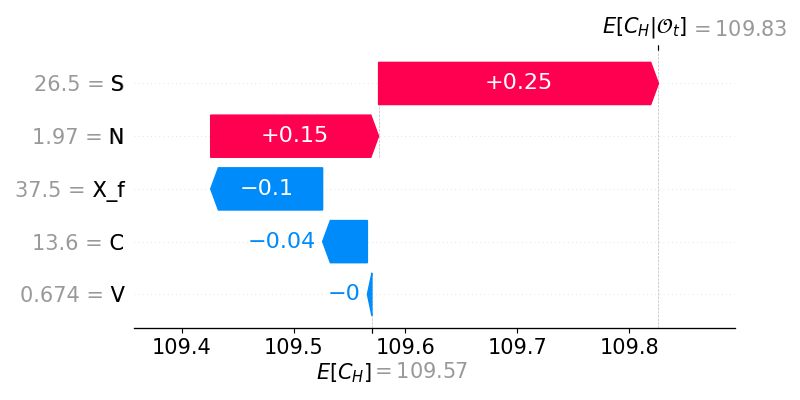
(a) SV score for observation of Batch 5.

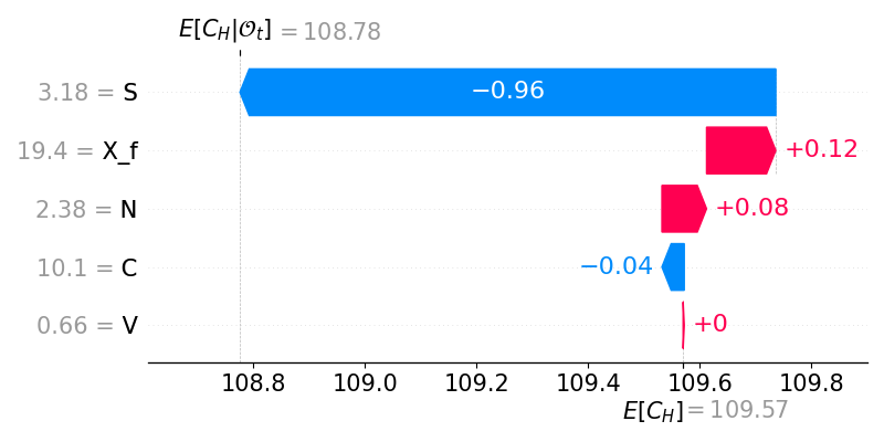
(b) SV score for observation of Batch 8.

Figure 5: Contribution of each dimension of the state variable to the model output $f(x)$ at 60 hours (corresponding to $t=15$).

Figure 5 shows how each input $x\in\mathcal{O}_{t}$ contributes to pushing the model output from $\mu_{H}^{C}={\mathbb{E}}[C_{H}]$ to ${\mathbb{E}}[C_{H}|\mathcal{O}_{t}]$. Positive contributions are in red, while negative contributions are in blue. In Case (a) corresponding to Batch 5, given the input observation $\mathcal{O}_{t}=(X_{ft},C_{t},S_{t},N_{t},V_{t})=(37.5,13.6,26.5,1.97,0.674)$ at 60 hours ($t=15$), the model predicts a final citrate concentration of 109.83 g/L under the DBN-RL policy. The main factor that pushes the prediction higher is the current substrate concentration $S_{t}=26.5$ g/L and nitrogen $N_{t}=1.97$ g/L. The high cell mass $X_{ft}$ shows a slight negative effect on citrate production because citrate formulation is inhibited in high cell density. In Case (b), the dominant negative contribution comes from low substrate concentration $S_{t}=3.18$ g/L, which is expected to cause a $0.96$ g/L reduction in the final citrate concentration. According to scientists, this result agrees with their experiment outcome: Batch 8 was known to have low oil feed (see Figure 3) which negatively impacted citrate productivity. The cell mass $X_{ft}=19.4$ and nitrogen $N=2.38$ increase the expected final citrate concentration by 0.12 g/L and 0.08 g/L respectively. In this way, we see how Shapley value analysis can be integrated with the DBN framework to quantify the effect of each individual component of the state variable on long-term outcomes.

6.5 Applying DBN-RL to Integrated Manufacturing Process Control

We present additional numerical results to illustrate how DBN-RL can support integrated biomanufacturing process control consisting of both upstream (fermentation) and downstream (purification) operations. The output of fermentation is a batch mixture containing both the product of interest and a significant amount of undesired impurity derived from the host cells and fermentation medium. This mixture then undergoes purification, which consists of one centrifugation and two precipitation steps.

The fermentation process is as described in Section 6.1. The downstream operation uses a two-dimensional state $\boldsymbol{s}=\left(\log P,\log I\right)$, where $(P,I)=(C,X_{f}+S+N)$ denote the respective concentration of citrate product and aggregated impurity. The log transformation is used to make it easier to linearize the process dynamics. Because the particle sizes of whole cells or cell debris are relatively large, centrifugation yields good separation of $X_{f}$ and has the output state $(P,I)=(C,\xi X_{f}+S+N)$, where $\xi=0.01$ denotes the separation efficiency. Both precipitation steps involve one scalar continuous CPP action $a=\log\zeta$, where $\zeta$ represents ammonium sulphate saturation. The complete specification of the process dynamics and state transition for purification is deferred to Appendix E.

The inherent stochastic uncertainty and initial state are set in the same way as in Section 6.1. The new process knowledge graph (encompassing both upstream and downstream operations) consists of 233 nodes and 818 edges with 39 time measurement steps (36 upstream steps and 3 downstream steps). A typical biomanufacturing system often has a trade-off between yield and purity (Martagan et al. 2018), with higher productivity often corresponding to higher impurity which increases the downstream purification cost. To incorporate these competing considerations, we use the linear reward function

$$r(\boldsymbol{s}_{t},{a}_{t})= -15+1.3\log P_{t}-\log I_{t}, t=39$$ if (ending profit), (17)

$$r(\boldsymbol{s}_{t},{a}_{t})= -0.05a_{t}, 37\leq t\leq 38$$ if (purification), (18)

$$r(\boldsymbol{s}_{t},{a}_{t})= -534.52{a}_{t}, 0\leq t\leq 36$$ if (fermentation). (19)

Equations (18)-(19) reflect the fact that the operating cost is primarily driven by the substrate consumption in the fermentation process and the ammonium sulphate consumption in the purification process. Equation (17) maintains the purity quality requirement on the final product via a linear penalty on $\log I_{t}$.

Table 4: Mean and standard error (SE) of reward, yield and purity obtained by using DBN-RL, DDPG, and practice-based policy.

Algorithms		DBN-RL						DDPG						Practice-based
Sample Size	$\kappa$	Reward		Yield		Purity		Reward		Yield		Purity		Reward		Yield		Purity
		Mean	SE	Mean	SE	Mean	SE	Mean	SE	Mean	SE	Mean	SE	Mean	SE	Mean	SE	Mean	SE
$R=8$	10	-35.05	1.65	95.08	1.99	0.79	0.02	-	-	-	-	-	-	-35.32	1.35	95.48	2.26	0.81	0.01
	25	-33.35	1.81	96.83	1.89	0.80	0.02	-	-	-	-	-	-	-33.12	1.25	97.21	1.96	0.82	0.01
	$\infty$	-32.65	1.51	97.80	1.83	0.80	0.01	-	-	-	-	-	-	-33.02	1.20	97.88	2.02	0.82	0.01
$R=15$	10	-33.05	1.70	99.08	1.41	0.80	0.02	-56.50	2.01	35.13	8.01	0.64	0.05	-	-	-	-	-	-
	25	-31.35	1.13	100.08	1.41	0.81	0.02	-50.00	1.93	40.09	7.91	0.66	0.04	-	-	-	-	-	-
	$\infty$	-31.05	1.31	99.80	1.63	0.80	0.02	-48.00	2.03	44.09	7.72	0.65	0.04	-	-	-	-	-	-
$R=50$	10	-31.88	1.37	104.88	1.63	0.81	0.02	-56.50	2.01	35.13	8.01	0.64	0.05	-	-	-	-	-	-
	25	-30.01	1.35	105.14	0.99	0.82	0.02	-50.00	1.93	40.09	7.91	0.66	0.04	-	-	-	-	-	-
	$\infty$	-29.05	1.11	106.89	1.63	0.82	0.01	-48.00	2.03	44.09	7.72	0.65	0.04	-	-	-	-	-	-
$R=100$	10	-30.91	1.24	105.78	1.41	0.81	0.01	-51.04	2.05	40.13	7.91	0.65	0.05	-	-	-	-	-	-
	25	-29.84	1.33	107.90	1.09	0.82	0.01	-46.88	2.10	44.09	7.34	0.67	0.04	-	-	-	-	-	-
	$\infty$	-29.05	1.01	107.69	0.93	0.83	0.01	-46.32	1.77	45.09	7.02	0.66	0.04	-	-	-	-	-	-
$R=400$	10	-29.79	1.52	108.13	1.48	0.84	0.01	-49.04	2.08	39.91	7.91	0.63	0.05	-	-	-	-	-	-
	25	-28.99	1.32	110.60	1.34	0.84	0.01	-48.53	1.99	44.70	7.34	0.69	0.04	-	-	-	-	-	-
	$\infty$	-28.49	1.22	113.13	1.27	0.83	0.01	-45.64	1.85	45.55	7.02	0.67	0.03	-	-	-	-	-	-

We compare the performance of DBN-RL with DDPG and experimental practice. DDPG was developed for stationary MDP settings and thus does not allow the state space to change from fermentation to purification. To handle this issue, we trained a separate DDPG agent for the purification process using the reward function (17)-(19). Then, in the integrated biomanufacturing process, the feed rate in fermentation was chosen by following the fermentation DDPG policy obtained in Section 6.2, and the purification decision was chosen by following the purification DDPG policy.

The practice-based policy was designed as follows. In the fermentation step, we use the same “human” policy as in Section 6.2. In the purification step, since we do not have access to laboratory data, we instead implemented the practice-based rule of Varga et al. (2001).

Table 4 reports the results of these approaches, including total reward, yield (citrate concentration after purification) and the final product purity ${P_{H}}/{(P_{H}+I_{H})}$. The results from DBN-RL and DDPG are based on 30 macro-replications. With a small sample size $R=8$, DBN-RL is competitive with the practice-based policy, and shows improved performance as $R$ increases. DDPG is much less sample-efficient, similar to what we saw before.

7 Conclusion

We have presented new models and algorithms for optimization of control policies on a Bayesian knowledge graph. This approach is especially effective in engineering problems with complex structure derived from physics models. Such structure can be partially extracted and turned into a prior for the Bayesian network. Furthermore, mechanistic models can also be used to provide additional information, which becomes very valuable in the presence of highly complex nonlinear dynamics with very small amounts of available pre-existing data. All of these issues arise in the domain of biomanufacturing, and we have demonstrated that our approach outperforms a state-of-the-art model-free RL method empirically.

As synthetic biology and biotechnology continue to adopt more complex processes for the generation of new drug products, from monoclonal antibodies (mAbs) to cell/gene therapies, data-driven and model-based control will become increasingly important. This work presents compelling evidence that model-based reinforcement learning can provide competitive performance and interpretability in the control of these important systems.

Appendix A Nomenclature

We list the symbols for the proposed DBN-RL framework in Table 5.

Table 5: List of Symbols

Variables	Description
$s_{t}^{k}$	the value of the $k$th state variable at time $t$
$a_{t}^{k}$	the value of the $k$th decision variable at time $t$
$\boldsymbol{s}_{t}$	the $n$-dimensional state vector
$\boldsymbol{a}_{t}$	the $m$-dimensional action vector
$\boldsymbol{\beta}^{s}_{t}$	$n\times n$ matrix of coefficients representing effects of $\boldsymbol{s}_{t}$ on $\boldsymbol{s}_{t+1}$
$\boldsymbol{\beta}^{a}_{t}$	$m\times n$ matrix of coefficients representing effects of $\boldsymbol{a}_{t}$ on $\boldsymbol{s}_{t+1}$
${\pi}_{\boldsymbol{\vartheta}_{t}}(\boldsymbol{s}_{t})$	linear deterministic nonstationary policy
$\boldsymbol{\vartheta}_{t}$	an $n\times m$ matrix of policy function coefficients
$r_{t}(\boldsymbol{s}_{t},\boldsymbol{a}_{t})$	linear reward function of state and action at time $t$
$m_{t}$	fixed cost at time $t$
$\boldsymbol{b}_{t}$	variable manufacturing cost
$\boldsymbol{c}_{t}$	purification penalty cost and product revenue
$\boldsymbol{w}$	DBN model parameters
$J\left(\pi;\boldsymbol{w}\right)$	expected total reward over the stochastic uncertainty given a model $\boldsymbol{w}$
$\mathcal{J}\left(\pi_{\boldsymbol{\theta}}\right)$	expected total reward over the stochastic uncertainty over the posterior distribution of $\boldsymbol{w}$
$\kappa$	reflecting different levels of stochastic uncertainty
$\mathcal{D}$	a set of process observations
$\eta_{k}$	stepsize of policy gradient optimization algorithm at the $k$th iteration
$\mathbb{C}$	closed convex feasible region
$B$	number of posterior samples
$R$	sample size of process observations
$\mu^{k}_{t}$	mean of $k$th state variable at time $t$
$v^{k}_{t}$	SD of $k$th state variable at time $t$
$\lambda_{t}^{k}$	mean of $k$th decision variable at time $t$
$\sigma^{k}_{t}$	SD of $k$th decision variable at time $t$
$\boldsymbol{\mu}^{a}_{t}$	mean action vector at time $t$
$\boldsymbol{\mu}^{s}_{t}$	mean state vector at time $t$
$\boldsymbol{\tau}$	process trajectory
$\mathbf{R}_{i,t}$	product of pathway coefficients from time step $i$ to $t$.
$H$	planning horizon
$P$	product (citrate) concentration at purification step
$I$	impurity concentration at purification step
$X_{f}$	lipid-free cell mass
$C$	citrate, the actual “product” generated by the cells’ metabolism
$S$	amount of substrate
$N$	amount of nitrogen
$V$	working volume of the entire batch
$F_{S}$	feed rate, or the amount of new substrate given to the cell in one unit of time
$\mathcal{O}_{h}$	set of inputs (i.e., state $\boldsymbol{s}_{h}$ and $\boldsymbol{a}_{h}$) at time step $h$
$\mbox{Sh}\left(\boldsymbol{s}_{t+1}|{o_{h}};\boldsymbol{w}\right)$	Shapley value of any input $o_{h}\in\mathcal{O}_{h}$ with respective to the expected future state of $\boldsymbol{s}_{t+1}$ with $t\geq h$

Appendix B Taylor Approximation for ODE-based Kinetic Models

This section shows how our proposed DBN model can be built using a first-order Taylor approximation of an ODE-based kinetic model. The biomanufacturing literature generally uses kinetic models based on PDEs or ODEs to model the dynamics of these variables. Suppose that $\boldsymbol{s}_{t}$ evolves according to the ordinary differential equation

$$\frac{d\boldsymbol{s}_{t}}{dt}=\boldsymbol{f}(\boldsymbol{s}_{t},\boldsymbol{a}_{t})$$ (20)

where $\boldsymbol{f}(\cdot)=(f_{1},f_{2},\ldots,f_{n})$ encodes the causal interdependencies between various CPPs and CQAs. One typically assumes that the functional form of $\boldsymbol{f}$ is known, though it may also depend on additional parameters that are calibrated from data. Supposing that the bioprocess is monitored on a small time scale using sensors, let us replace (20) by the first-order Taylor approximation

$$\frac{\Delta\boldsymbol{s}_{t+1}}{\Delta t}=\boldsymbol{f}(\boldsymbol{\mu}_{t}^{s},\boldsymbol{\mu}_{t}^{a})+J^{s}_{f}(\boldsymbol{\mu}_{t}^{s})(\boldsymbol{s}_{t}-\boldsymbol{\mu}_{t}^{s})+J^{a}_{f}(\boldsymbol{\mu}_{t}^{a})(\boldsymbol{a}_{t}-\boldsymbol{\mu}_{t}^{a}),$$ (21)

where $\Delta\boldsymbol{s}_{t+1}=\boldsymbol{s}_{t+1}-\boldsymbol{s}_{t}$, and $J^{s}_{f},J^{a}_{f}$ denote the Jacobian matrices of $\boldsymbol{f}$ with respect to $\boldsymbol{s}_{t}$ and $\boldsymbol{a}_{t}$, respectively. The interval $\Delta t$ can change with time, but we keep it constant for simplicity. The approximation is taken at a point $\left(\boldsymbol{\mu}_{t}^{s},\boldsymbol{\mu}_{t}^{a}\right)$ to be elucidated later. We can then rewrite (21) as

$$\boldsymbol{s}_{t+1}=\boldsymbol{\mu}_{t}^{s}+\Delta t\cdot\boldsymbol{f}(\boldsymbol{\mu}_{t}^{s},\boldsymbol{\mu}_{t}^{a})+(\Delta t\cdot J_{f}(\boldsymbol{\mu}_{t}^{s})+1)(\boldsymbol{s}_{t}-\boldsymbol{\mu}_{t}^{s})+\Delta t\cdot J_{f}(\boldsymbol{\mu}_{t}^{a})(\boldsymbol{a}_{t}-\boldsymbol{\mu}_{t}^{a})+R_{t+1},$$ (22)

where $R_{t+1}$ is a remainder term modeling the effect from other uncontrolled factors. In this way, the original process dynamics have been linearized, with $R_{t+1}$ serving as a residual. One can easily represent (22) using a network model. An edge exists from $s^{k}_{t}$ (respectively, $a^{k}_{t}$) to $s^{l}_{t+1}$ if the $\left(k,l\right)$th entry of $J^{s}_{f}$ (respectively, $J^{a}_{f}$) is not identically zero. The linearized dynamics can provide prior knowledge to the state transition model of the dynamic Bayesian network. Specifically, (1) has the same form as (22) if we let

$$\boldsymbol{\mu}_{t+1}^{s}=\boldsymbol{\mu}_{t}^{s}+\Delta t\cdot\boldsymbol{f}(\boldsymbol{\mu}_{t}^{s},\boldsymbol{\mu}_{t}^{a}),~{}~{}~{}\boldsymbol{\beta}_{t}^{s}=\Delta t\cdot J_{f}(\boldsymbol{\mu}_{t}^{s})+1,~{}~{}~{}\boldsymbol{\beta}_{t}^{a}=\Delta t\cdot J_{f}(\boldsymbol{\mu}_{t}^{a}),$$

and treat $R_{t+1}$ as the residual.

Appendix C Details of Gibbs Sampling Procedure

This section briefly describes key computations used in the Gibbs sampling procedure. Given the data $\mathcal{D}$, the posterior distribution of $\boldsymbol{w}$ is proportional to $p\left(\boldsymbol{w}\right)\prod_{n=1}^{R}p\left(\boldsymbol{\tau}^{(n)}|\boldsymbol{w}\right)$. The Gibbs sampling technique can be used to sample from this distribution. Overall, the procedure is quite similar to the one laid out in Xie et al. [2020], so we will only give a brief description of the computations used in our setting.

For each node $X$ in the network, let $Ch\left(X\right)$ be the set of child nodes (direct successors) of $X$. The full likelihood $p\left(\mathcal{D}|\boldsymbol{w}\right)$ becomes

$$p(\mathcal{D}|\boldsymbol{w})=\prod^{R}_{i=1}p(\boldsymbol{\tau}_{i}|\boldsymbol{w})=\prod^{R}_{i=1}\prod_{t=1}^{H}\left[\prod_{k=1}^{m}\mathcal{N}\left(\lambda^{k}_{t},(\sigma^{k}_{t})^{2}\right)\prod_{k=1}^{n}\mathcal{N}\left(\mu^{k}_{t+1}+\sum_{X^{j}_{t}\in Pa(s^{k}_{t+1})}\beta^{jk}_{t}(X^{j}_{t}-\mu^{j}_{t}),(v^{k}_{t+1})^{2}\right)\right],$$

For the model parameters $\boldsymbol{\mu}^{a},\boldsymbol{\mu}^{s},\boldsymbol{\sigma}^{2}\boldsymbol{v}^{2},\boldsymbol{\beta}$, we have the conjugate prior

$$p(\boldsymbol{\mu}^{a},\boldsymbol{\mu}^{s},\boldsymbol{\sigma}^{2}\boldsymbol{v}^{2},\boldsymbol{\beta})=\prod_{t=1}^{H}\left(\prod_{k=1}^{m}p(\lambda^{k}_{t})p((\sigma_{k}^{t})^{2})\prod_{k=1}^{n}p(\mu^{k}_{t})p((v^{k}_{t})^{2})\prod_{i\neq j}p(\beta^{ij}_{t})\right),$$

where

$$p(\lambda^{k}_{t}) = \mathcal{N}\left({\lambda}^{k(0)}_{t},\left({\delta}_{t,k}^{(\lambda)}\right)^{2}\right),\quad p(\mu^{k}_{t})=\mathcal{N}\left({\mu}^{k(0)}_{t},\left({\delta}_{t,k}^{(\mu)}\right)^{2}\right),\quad p(\beta_{t}^{ij})=\mathcal{N}\left({\beta}_{t}^{ij(0)},\left({\delta}_{t,ij}^{(\beta)}\right)^{2}\right)$$

$$p\left((\sigma_{t}^{k})^{2}\right) = \mbox{Inv-}\Gamma\left(\dfrac{\kappa_{t,k}^{(\sigma)}}{2},\dfrac{\rho_{t,k}^{(\sigma)}}{2}\right),\quad p((v_{t}^{k})^{2})=\mbox{Inv-}\Gamma\left(\dfrac{\kappa_{t,k}^{(v)}}{2},\dfrac{\rho_{t,k}^{(v)}}{2}\right),$$

where $\mbox{Inv-}\Gamma$ denotes the inverse-gamma distribution.

We now state the posterior conditional distribution for each model parameter; the detailed derivations are omitted since they proceed very similarly to those in Xie et al. [2020]. Let $\boldsymbol{\mu}^{a}_{-t,k}$, $\boldsymbol{\mu}^{s}_{-t,k}$, $\boldsymbol{\sigma}_{-t,k}^{2}$, $\boldsymbol{v}_{-t,k}^{2}$ and $\boldsymbol{\beta}_{-t,jk}$ denote the collection of parameters $\boldsymbol{\mu}^{a},\boldsymbol{\mu}^{s},\boldsymbol{\sigma},\boldsymbol{v},\boldsymbol{\beta}$ excluding the $k$th or ${(j,k)}$th element at time $t$. These collections are used to obtain five conditional distributions:

• $p(\beta^{jk}_{t}|\mathcal{D},\boldsymbol{\mu}^{a},\boldsymbol{\mu}^{s},\boldsymbol{\sigma}^{2},\boldsymbol{v}^{2},\boldsymbol{\beta}_{-t,jk})=\mathcal{N}(\tilde{\beta}_{t}^{jk},(\tilde{\delta}_{t,jk}^{(\beta)})^{2})$, where

  $$\tilde{\beta}_{t}^{jk} = \dfrac{({\delta}_{t,jk}^{(\beta)})^{2}\sum_{i=1}^{R}\alpha_{t}^{j(i)}m_{t+1,jk}^{(i)}+(v_{t+1}^{k})^{2}{\beta}_{t}^{ij(0)}}{({\delta}_{t,jk}^{(\beta)})^{2}\sum_{i=1}^{R}(\alpha_{t}^{j(i)})^{2}+(v_{t+1}^{k})^{2}}$$

  $$\tilde{\delta}_{t,jk}^{(\beta)2} = \dfrac{({\delta}_{t,jk}^{(\beta)})^{2}(v_{t+1}^{k})^{2}}{({\delta}_{t,jk}^{(\beta)})^{2}\sum_{i=1}^{R}(\alpha_{t}^{j(i)})^{2}+(v_{t+1}^{k})^{2}}$$

  with $\alpha_{t}^{j(i)}=x_{t}^{j(i)}-\mu_{t}^{j}$ and $m_{t+1,jk}^{(i)}=(s_{t+1}^{k(i)}-\mu_{t+1}^{k})-\sum_{X_{t}^{\ell}\in Pa(s_{t+1}^{k})/\{x_{t}^{j}\}}\beta_{t}^{\ell k}(x_{t}^{\ell(i)}-\mu_{t}^{\ell})$.

• $p\left((v_{t}^{k})^{2}|\mathcal{D},\boldsymbol{\mu}^{a},\boldsymbol{\mu}^{s},\boldsymbol{\sigma}^{2},\boldsymbol{v}_{-t,k}^{2},\boldsymbol{\beta}\right)=\mbox{Inv-}\Gamma\left(\dfrac{\tilde{\kappa}_{t,k}^{(v)}}{2},\dfrac{\tilde{\rho}_{t,k}^{(v)}}{2}\right)$, where

  $$\tilde{\kappa}_{t,k}^{(v)} = \kappa_{t,k}^{(v)}+R,\qquad\tilde{\rho}_{t,k}^{(v)}=\rho_{t,k}^{(v)}+\sum_{i=1}^{R}u_{t,k}^{(i)2},$$

  $$u_{t,k}^{(i)} = (s_{t}^{k(i)}-\mu_{t}^{k})-\sum_{X_{t}^{j}\in Pa(s_{t}^{k})}\beta_{t}^{jk}(x_{t}^{j(i)}-\mu_{t}^{j}).$$

• $p\left((\sigma_{t}^{k})^{2}|\mathcal{D},\boldsymbol{\mu}^{a},\boldsymbol{\mu}^{s},\boldsymbol{\sigma}_{-t,k}^{2},\boldsymbol{v}^{2},\boldsymbol{\beta}\right)=\mbox{Inv-}\Gamma\left(\dfrac{\tilde{\kappa}_{t,k}^{(\sigma)}}{2},\dfrac{\tilde{\rho}_{t,k}^{(\sigma)}}{2}\right)$, where

  $$\tilde{\kappa}_{t,k}^{(\sigma)}=\kappa_{t,k}^{(\sigma)}+R,\quad\tilde{\rho}_{t,k}^{(\sigma)}=\rho_{t,k}^{(\sigma)}+\sum_{i=1}^{R}u_{t,k}^{(i)2},\quad u_{t,k}^{(i)}=s_{t}^{k(i)}-\mu_{t}^{k}.$$

• $p\left(\mu_{t}^{k}|\mathcal{D},\boldsymbol{\mu}^{a},\boldsymbol{\mu}^{s}_{-t,k},\boldsymbol{\sigma}^{2},\boldsymbol{v}^{2},\boldsymbol{\beta}\right)=\mathcal{N}(\tilde{\mu}_{t}^{k},(\tilde{\delta}_{t,k}^{(\mu)})^{2})$, where

  $$\tilde{\mu}_{t}^{k} = (\tilde{\delta}_{t,k}^{(\mu)})^{2}\left[\dfrac{\mu_{t}^{k(0)}}{({\delta}_{t,k}^{(\mu)})^{2}}+\sum_{i=1}^{R}\dfrac{a_{t,k}^{(i)}}{(v_{t}^{k})^{2}}+\sum_{i=1}^{R}\sum_{s_{t+1}^{\ell}\in Ch(s_{t}^{k})}\dfrac{\beta_{t}^{k\ell}c_{t,k\ell}^{(i)}}{(v_{t}^{\ell})^{2}}\right]$$

  $$\dfrac{1}{(\tilde{\delta}_{t,k}^{(\mu)})^{2}} = \dfrac{1}{({\delta}_{t,k}^{(\mu)})^{2}}+\dfrac{R}{(v_{t}^{k})^{2}}+\sum_{s_{t+1}^{\ell}\in Ch(s_{t}^{k})}\dfrac{R(\beta_{t}^{k\ell})^{2}}{(v_{t}^{\ell})^{2}},$$

  with

  $$a_{t,k}^{(i)} = s_{t}^{k(i)}-\sum_{X_{t-1}^{j}\in Pa(s_{t}^{k})}\beta_{t-1}^{jk}(x_{t-1}^{j(i)}-\mu_{t-1}^{j})$$

  $$c_{t,k\ell}^{(i)} = \beta_{t}^{k\ell}s_{t}^{k(i)}-(s_{t+1}^{\ell(i)}-\mu_{t+1}^{\ell})+\sum_{X_{t}^{j}\in Pa(s_{t+1}^{\ell})/\{s_{t}^{k}\}}\beta_{t}^{j\ell}(x_{t}^{j(i)}-\mu_{t}^{j}).$$

• $p\left(\lambda_{t}^{k}|\mathcal{D},\boldsymbol{\mu}^{a}_{-t,k},\boldsymbol{\mu}^{s},\boldsymbol{\sigma}^{2},\boldsymbol{v}^{2},\boldsymbol{\beta}\right)=\mathcal{N}(\tilde{\lambda}_{t}^{k},(\tilde{\delta}_{t,k}^{(\lambda)})^{2})$, where

  $$\tilde{\lambda}_{t}^{k} = (\tilde{\delta}_{t,k}^{(\lambda)})^{2}\left[\dfrac{\lambda_{t}^{k(0)}}{({\delta}_{t,k}^{(\lambda)})^{2}}+\sum_{i=1}^{R}\dfrac{a_{t}^{k(i)}}{(v_{t}^{k})^{2}}+\sum_{i=1}^{R}\sum_{s_{t+1}^{\ell}\in Ch(a_{t}^{k})}\dfrac{\beta_{t}^{k\ell}c_{t,k\ell}^{(i)}}{(v_{t}^{\ell})^{2}}\right]$$

  $$\dfrac{1}{(\tilde{\delta}_{t,k}^{(\lambda)})^{2}} = \dfrac{1}{({\delta}_{t,k}^{(\lambda)})^{2}}+\dfrac{R}{(v_{t}^{k})^{2}}+\sum_{s_{t+1}^{\ell}\in Ch(a_{t}^{k})}\dfrac{R(\beta_{t}^{k\ell})^{2}}{(v_{t}^{\ell})^{2}}$$

  with

  $$c_{t,k\ell}^{(i)}=\beta_{t}^{k\ell}a_{t}^{k(i)}-(s_{t+1}^{\ell(i)}-\mu_{t+1}^{\ell})+\sum_{X_{t}^{j}\in Pa(s_{t+1}^{\ell})/\{a_{t}^{k}\}}\beta_{t}^{j\ell}(x_{t}^{j(i)}-\mu_{t}^{j}).$$

In Gibbs sampling, we set a prior $p\left(\boldsymbol{w}\right)$ and sample $\boldsymbol{w}^{(0)}$ from it. Now, given $\boldsymbol{w}^{(i-1)}$ we sequentially compute and generate one sample from the above conditional posterior distributions for each parameter, obtaining a new $\boldsymbol{w}^{(i)}$. By repeating this process, one can arrive at a sample whose distribution is a very close approximation to the desired posterior.

Appendix D Kinetic Modeling of Fed-Batch Fermentation of Yarrowia lipolytica

Here we provide additional domain information about the upstream fermentation studied in Section 6.1; specifically, the complete details of the kinetic models used to construct the Bayesian network. Cell growth and citrate production of Yarrowia lipolytica take place inside a bioreactor, which requires carbon sources (e.g., soybean oil or waste cooking oil), nitrogen (yeast extract and ammonia sulfate), and oxygen, subject to good mixing and carefully controlled operating conditions (e.g., pH, temperature). During fermentation, the feed rate is adjusted to control the concentration of oil.

In our case study, we treat feed rate as the only control. Other CPPs relevant to the bioprocess are set automatically as follows. The dissolved oxygen level is set at $30\%$ of air saturation using cascade controls of agitation speed between 500 and 1,400 rpm, with the aeration rate fixed at 0.3 L/min. The pH is controlled at 6.0 for the first $12$ hours, then maintained at $7.0$ until the end of the process. The temperature is maintained at $30^{\circ}$C for the entire run. We stop the fermentation process after 140 hours (or if the volume reaches the bioreactor capacity).

The kinetics of the fed-batch fermentation of Yarrowia lipolytica can be described by a system of differential equations. The biomanufacturing literature uses deterministic ODEs, but we have augmented some of the equations with Brownian noise terms of the form $dB_{t}$ to reflect the inherent stochastic uncertainty of the bioprocess. Table 6 provides a list of environmental parameters that appear in the equations, together with their values in our case study. The equations themselves can be grouped into eight parts as follows:

Table 6: Mechanistic model parameter description and estimation.

Parameters	Descrption	Estimation	Unit
$\alpha_{L}$	Coefficient of lipid production for cell growth	0.1273	-
$C_{max}$	Maximum citrate concentration that cells can tolerate	130.90	g/L
$K_{iN}$	Nitrogen limitation constant to trigger on lipid and citrate production	0.1229	g/L
$K_{iS}$	Inhibition constant for substrate in lipid-based growth kinetics	612.18	g/L
$K_{iX}$	Constant for cell density effect on cell growth and lipid/citrate formation	59.974	g/L
$K_{N}$	Saturation constant for intracellular nitrogen in growth kinetics	0.0200	g/L
$K_{O}$	Saturation constant for dissolved oxygen in kinetics of cell growth, substrate uptake, lipid consumption by $\beta$-oxidation	0.3309	% Air
$K_{S}$	Saturation constant for substrate utilization	0.0430	g/L
$K_{SL}$	Coefficient for lipid consumption/decomposition	0.0217	-
$m_{s}$	Maintenance coefficient for substrate	0.0225	g/g/h
$r_{L}$	Constant ratio of lipid carbon flow to total carbon flow (lipid + citrate)	0.4792	-
$V_{evap}$	Evaporation rate (or loss of volume) in the fermentation	0.0026	L/h
$Y_{cs}$	Yield coefficient of citrate based on substrate consumed	0.6826	g/g
$Y_{ls}$	Yield coefficient of lipid based on substrate consumed	0.3574	g/g
$Y_{xn}$	Yield coefficient of cell mass based on nitrogen consumed	10.0	g/g
$Y_{xs}$	Yield coefficient of cell mass based on substrate consumed	0.2386	g/g
$\beta_{LCmax}$	Coefficient of maximum carbon flow for citrate and lipid	0.1426	h-1
$\mu_{max}$	Maximum specific growth rate on substrate	0.3845	h-1
$S_{F}$	Oil concentration in oil feed	917.00	g/L

1. Cell mass: The total cell mass $X$ consists of lipid-free ($X_{f}$) and lipid ($L$) mass, and is measured by dry cell weight (DCW) in fermentation experiments.

   $$X =X_{f}+L$$

2. Dilution rate: The dilution $D$ of the working liquid volume in the bioreactor is caused by feed of base, such as KOH solution ($F_{B}$) and substrate ($F_{S}$):

   $$D =\frac{F_{B}+F_{S}}{V}$$

3. Lipid-free cell growth: Cell growth consumes nutrients, including the substrate (carbon source) $S$, nitrogen $N$, and dissolved oxygen $O$, and is described by coupled Monod equations, with considerations of inhibitions from high oil concentrations and cell densities:

   $$\mbox{d}X_{f} =\mu X_{f}\mbox{d}t-\left(D-\frac{V_{evap}}{V}\right)X_{f}\mbox{d}t+\sigma(X_{f})\mbox{d}B_{t}$$

   $$\mu =\mu_{max}\left(\frac{S}{K_{S}+S}\cdot\frac{1}{1+S/K_{iS}}\right)\frac{N}{K_{N}+N}\cdot\frac{O}{K_{O}+O}\cdot\frac{1}{1+X_{f}/K_{ix}}$$

4. Citrate accumulation: Citrate ($C$) is an overflow of all the carbon introduced to the lipid synthesis pathway ($\beta_{LC}$), which is more active under nitrogen-limited, substrate-rich, and aerobic conditions. Only a proportion $r_{L}$ of the total carbon flow (citrate plus lipid) in the lipid synthesis pathway goes to production due to the overflow loss in citrate. A tolerance limit $C_{max}$ of citrate, and the effect of cell density on product formation ($1/(1+X_{f}/K_{iX})$), are also considered in the model.

   $${\mbox{d}C} =\beta_{C}\cdot X_{f}\mbox{d}t-\left(D-\frac{V_{evap}}{V}\right)C\mbox{d}t+\sigma(C)\mbox{d}B_{t}$$

   $$\beta_{C} =2(1-r_{L})\beta_{LC}$$

   $$\beta_{LC} =\frac{1}{1+N/K_{iN}}\cdot\left(\frac{S}{K_{S}+S}\cdot\frac{1}{1+S/K_{iS}}\right)\frac{O}{K_{O}+O}\cdot\frac{1}{1+X_{f}/K_{iX}}\left(1-\frac{C}{C_{max}}\right)\beta_{LCmax}$$

5. Lipid accumulation: Lipid is accumulated under nitrogen-limited, substrate-rich, and aerobic conditions. Lipid production is described using partial growth-association kinetics; a small portion of lipid can be degraded when its concentration is high in the presence of oxygen.

   $$\mbox{d}{L} =q_{L}\cdot X_{f}\mbox{d}t-\left(D-\frac{V_{evap}}{V}\right)L\mbox{d}t+\sigma(L)\mbox{d}B_{t}$$

   $$=\left(\alpha_{L}\cdot\mu+\beta_{L}\right)X_{f}\mbox{d}t-\left(D-\frac{V_{evap}}{V}\right)L\mbox{d}t+\sigma(L)\mbox{d}B_{t}$$

   $$\beta_{L} =r_{L}\cdot\beta_{LC}-K_{SL}\frac{L}{L+X_{f}}\cdot\frac{O}{K_{O}+O}$$

6. Substrate consumption: Oil ($S$) is fed during the fed-batch fermentation and used for cell growth, energy maintenance, citrate formation, and lipid production.

   $$-{dS} =q_{S}\cdot X_{f}\mbox{d}t-\frac{F_{S}}{V}S_{F}\mbox{d}t+\left(D-\frac{V_{evap}}{V}\right)S\mbox{d}t+\sigma(S)\mbox{d}B_{t}$$

   $$q_{S} =\frac{1}{Y_{X/S}}\mu+\frac{O}{K_{O}+O}\cdot\frac{S}{K_{S}+S}m_{S}+\frac{1}{Y_{C/S}}\beta_{C}+\frac{1}{Y_{L/S}}\beta_{L}$$

7. Nitrogen consumption: Extracellular nitrogen ($N$) is used for cell growth.

   $$-{dN} =\frac{1}{Y_{X/N}}\mu X_{f}\mbox{d}t+(D-\frac{V_{evap}}{V})N\mbox{d}t+\sigma(N)\mbox{d}B_{t}$$

8. Volume change: The rate $V$ of working volume change of the fermentation is calculated based on the rates of base feed ($F_{B}$), substrate feed ($F_{S}$), and evaporation ($V_{evap}$).

   $${dV} =(F_{B}+F_{S}-V_{evap})\mbox{d}t+\sigma(V)\mbox{d}B_{t}$$

   $$F_{B} =\frac{V}{1000}\left(\frac{7.14}{Y_{X/N}}\mu X_{f}+1.59\beta_{C}X_{f}\right)$$

Figure 3 in the main text shows the fit of the ODE trajectory to the 8 available batches of experimental data. The fit is not perfect due to the limited sample size and the noticeably large variation between experimental trajectories (a consequence of the fact that scientists conducted these experiments with very different oil feeding profiles).

Appendix E Purification Process Dynamics in Integrated Process Control

This section provides details about the downstream operation added in Section 6.5. Similarly to Appendix D, we develop a mechanistic model of the purification process during the production of citrate acid. The downstream process described here is a simplified version of what is given in Varga et al. [2001]. It contains multiple stages, including: (C1) disc stack centrifugation for cell debris removal; (P1) a first ammonium sulphate precipitation stage to selectively precipitate undesired impurities; and (P2) a second ammonium sulphate precipitation to selectively precipitate the desired product. In the downstream setup, sensors are only placed at the entrance and exit of each stage.

As the particle sizes of whole cell or cell debris are relatively large, we expect Stage (C1) to yield good separation of the material. Thus, given the output $(X_{f},C,S,N)$ of the upstream fermentation process, we obtain the following aggregated process state after centrifugation:

$$\mbox{(C1)}\quad(P,I)=(C,\xi X_{f}+S+N)$$ (23)

where $P$ denotes the total amount of product, $I$ denotes the total amount of impurity, and $\xi=0.01$ denotes the separation efficiency of cell debris in Stage (C1).

Next, we discuss the ammonium sulphate precipitation steps (P1) and (P2). Purification through precipitation involves a trade-off between yield and purity, illustrated in Figure 6. The operator needs to decide the ammonium sulphate saturation to remove as much impurity and as little product as possible. In this example, the operator selects low ammonium sulphate saturation (40%-50%) to precipitate the undesired impurity in Step (P1) and selects high ammonium sulphate saturation (60%-80%) to selectively precipitate the product in Step (P2). Thus, in (P1), the precipitation process keeps more product but removes less impurity if lower ammonium sulphate saturation is used; and in (P2), the process precipitates or keeps more product but removes more impurity if lower ammonium sulphate saturation is used.

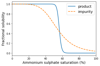
Figure 6: Fractional solubility of product and impurity.

The fractional ammonium sulphate solubility of natural product and impurity from yeast have been described by Niktari et al. [1990] using the equation

$$F(\zeta)=\frac{1}{1+(\zeta/a)^{b}}\vspace{-0.1in}$$ (24)

where $F$ is fractional solubility (the fraction of enzyme or protein that is soluble), $\zeta$ is the ammonium sulphate saturation and $a$, $b$ are constants. In the simulation model, we set the fractional solubility parameters as $a=56.27$, $b=42.00$ for product and $a=53.72$, $b=5.23$ for impurity. Thus the nonlinear relationships of process states before and after stages (P1) and (P2) are given by

$$\mbox{(P1)}\quad P_{t+1} =F_{P}(\zeta_{t})\cdot P_{t},\quad I_{t+1}=F_{I}(\zeta_{t})\cdot I_{t}$$ (25)

$$\mbox{(P2)}\quad P_{t+1} =(1-F_{P}(\zeta_{t}))\cdot P_{t},\quad I_{t+1}=(1-F_{I}(\zeta_{t}))\cdot I_{t}$$ (26)

where $F_{P}(\zeta)$ and $F_{I}(\zeta)$ denote the fractional solubility model in (24) for product and impurity respectively. Then by taking logarithms and including normally distributed residual terms, the nonlinear state transition (25)-(26) becomes

$$\mbox{(P1)}\quad\log P_{t+1} =\log F_{P}(\zeta_{t})+\log P_{t}+e^{P}_{t},\quad\log I_{t+1}=\log F_{I}(\zeta_{t})+\log I_{t}+e^{I}_{t}$$

$$\mbox{(P2)}\quad\log P_{t+1} =\log\left(1-F_{P}(\zeta_{t})\right)+\log P_{t}+e^{P}_{t},\quad\log I_{t+1}=\log\left(1-F_{I}(\zeta_{t})\right)+\log I_{t}+e^{I}_{t}.$$

This gives the state transition model for Phases (P1) and (P2) from state $(\log P_{t},\log I_{t})$ to next state $(\log P_{t+1},\log I_{t+1})$ after taking the action $\log\zeta_{t}$ in the precipitation processes.

Appendix F Proofs

In this section, we give the proofs and the derivations of all results stated in the main text.

F.1 Proof for Proposition 1

By plugging in the linear policy function (6) into the state transition in (1), we have

$$\boldsymbol{s}_{t+1} = \boldsymbol{\mu}_{t+1}^{s}+\left({\boldsymbol{\beta}_{t}^{s}}\right)^{\top}(\boldsymbol{s}_{t}-\boldsymbol{\mu}_{t}^{s})+\left(\boldsymbol{\beta}_{t}^{a}\right)^{\top}(\boldsymbol{a}_{t}-\boldsymbol{\mu}_{t}^{a})+V_{t+1}\mathbf{z}$$

$$= \boldsymbol{\mu}_{t+1}^{s}+\left(\boldsymbol{\beta}_{t}^{s}\right)^{\top}(\boldsymbol{s}_{t}-\boldsymbol{\mu}_{t}^{s})+\left(\boldsymbol{\beta}_{t}^{a}\right)^{\top}\left[\boldsymbol{\mu}^{a}_{t}+\boldsymbol{\vartheta}_{t}^{\top}(\boldsymbol{s}_{t}-\boldsymbol{\mu}_{t}^{s})-\boldsymbol{\mu}_{t}^{a}\right]+\boldsymbol{e}_{t+1}$$

$$= \boldsymbol{\mu}_{t+1}^{s}+\left(\left(\boldsymbol{\beta}_{t}^{s}\right)^{\top}+\left(\boldsymbol{\beta}_{t}^{a}\right)^{\top}\boldsymbol{\vartheta}_{t}^{\top}\right)(\boldsymbol{s}_{t}-\boldsymbol{\mu}^{s}_{t})+\boldsymbol{e}_{t+1}$$

$$= \boldsymbol{\mu}_{t+1}^{s}+(\left(\boldsymbol{\beta}_{t}^{s}\right)^{\top}+\left(\boldsymbol{\beta}_{t}^{a}\right)^{\top}\boldsymbol{\vartheta}_{t}^{\top})\left(\left(\boldsymbol{\beta}_{t-1}^{s}\right)^{\top}+\left(\boldsymbol{\beta}_{t-1}^{a}\right)^{\top}\boldsymbol{\vartheta}_{t-1}^{\top}\right)(\boldsymbol{s}_{t-1}-\boldsymbol{\mu}^{s}_{t-1})+\left[(\left(\boldsymbol{\beta}_{t}^{s}\right)^{\top}+\left(\boldsymbol{\beta}_{t}^{a}\right)^{\top}\boldsymbol{\vartheta}_{t}^{\top})\boldsymbol{e}_{t}+\boldsymbol{e}_{t+1}\right]$$

$$= \boldsymbol{\mu}_{t+1}^{s}+\mathbf{R}_{t-1,t}(\boldsymbol{s}_{t-1}-\boldsymbol{\mu}^{s}_{t-1})+\left[\left(\left(\boldsymbol{\beta}_{t}^{s}\right)^{\top}+\left(\boldsymbol{\beta}_{t}^{a}\right)^{\top}\boldsymbol{\vartheta}_{t}^{\top}\right)\boldsymbol{e}_{t}+\boldsymbol{e}_{t+1}\right]$$

$$\ldots$$

$$= \boldsymbol{\mu}_{t+1}^{s}+\prod_{i=1}^{t}\left(\left(\boldsymbol{\beta}_{i}^{s}\right)^{\top}+\left(\boldsymbol{\beta}_{i}^{a}\right)^{\top}\boldsymbol{\vartheta}_{i}^{\top}\right)(\boldsymbol{s}_{1}-\boldsymbol{\mu}^{s}_{1})+\left[\sum_{i=1}^{t}\left(\prod_{j=i}^{t}\left(\left(\boldsymbol{\beta}_{j}^{s}\right)^{\top}+\left(\boldsymbol{\beta}_{j}^{a}\right)^{\top}\boldsymbol{\vartheta}_{j}^{\top}\right)\boldsymbol{e}_{i}\right)+\boldsymbol{e}_{t+1}\right]$$ (28)

$$= \boldsymbol{\mu}_{t+1}^{s}+\mathbf{R}_{1,t}(\boldsymbol{s}_{1}-\boldsymbol{\mu}^{s}_{1})+\left[\sum_{i=1}^{t}\mathbf{R}_{i,t}\boldsymbol{e}_{i}+\boldsymbol{e}_{t+1}\right]\vspace{-0.1in}$$ (29)

where $\boldsymbol{e}_{t}$ is a $n$-dimensional normal random column vector with mean zero and diagonal covariance matrix $V_{t}\triangleq\mbox{diag}((v_{t}^{s})^{2})$. Similarly, one can expand $\boldsymbol{s}_{t+1}$ until time $h$ to obtain an analog of (28), which yields the desired result.

F.2 Proof for Proposition 2

The conditional mean follows directly from (29) above. Because the vectors $\boldsymbol{e}_{i},\boldsymbol{e}_{j}$ are mutually independent, we obtain

$$\mbox{Var}[\boldsymbol{s}_{t+1}|\boldsymbol{s}_{1},\boldsymbol{\pi}_{\boldsymbol{\theta}}] = \mbox{Var}\left[\sum_{i=1}^{t}\mathbf{R}_{i,t}\boldsymbol{e}_{i}+\boldsymbol{e}_{t+1}\right]=\sum_{i=1}^{t}\mathbf{R}_{i,t}\mbox{Var}\left[\boldsymbol{e}_{i}\right]\mathbf{R}_{i,t}^{\top}+\mbox{Var}\left[\boldsymbol{e}_{t+1}\right]=\sum_{i=1}^{t}\mathbf{R}_{i,t}V_{i}^{2}\mathbf{R}_{i,t}^{\top}+V_{t+1}^{2}.$$

The objective function can be obtained from (2) and (6) as,

$$J(\boldsymbol{\theta};\boldsymbol{w}) = \sum_{t=1}^{H}{\mathbb{E}}[r_{t}(\boldsymbol{s}_{t},\boldsymbol{a}_{t})|\boldsymbol{\pi}_{\boldsymbol{\theta}},\boldsymbol{s}_{1},\boldsymbol{w}]=\sum_{t=1}^{H}m_{t}+\boldsymbol{b}_{t}^{\top}\boldsymbol{a}_{t}+\boldsymbol{c}_{t}^{\top}{\mathbb{E}}[\boldsymbol{s}_{t}|\boldsymbol{\pi}_{\boldsymbol{\theta}},\boldsymbol{s}_{1},\boldsymbol{w}]$$

$$= \sum^{H}_{t=1}m_{t}+\boldsymbol{b}_{t}^{\top}\boldsymbol{\mu}^{a}_{t}+(\boldsymbol{b}_{t}^{\top}\boldsymbol{\vartheta}_{t}^{\top}+\boldsymbol{c}_{t}^{\top}){\mathbb{E}}[\boldsymbol{s}_{t}|\boldsymbol{s}_{1},\boldsymbol{\pi}_{\boldsymbol{\theta}}]-\boldsymbol{b}_{t}^{\top}\boldsymbol{\vartheta}^{\top}\boldsymbol{\mu}_{t}^{s}.$$

Plugging in the conditional mean computed previously, we obtain

$$J(\boldsymbol{\theta};\boldsymbol{w}) = \sum^{H}_{t=1}m_{t}+\boldsymbol{b}_{t}^{\top}\boldsymbol{\mu}^{a}_{t}+(\boldsymbol{b}_{t}^{\top}\boldsymbol{\vartheta}_{t}^{\top}+\boldsymbol{c}_{t}^{\top})(\boldsymbol{\mu}_{t}^{s}+\mathbf{R}_{1,t}(\boldsymbol{s}_{1}-\boldsymbol{\mu}_{1}^{s}))-\boldsymbol{b}_{t}^{\top}\boldsymbol{\vartheta}_{t}^{\top}\boldsymbol{\mu}^{s}_{t}$$

$$= \sum^{H}_{t=1}m_{t}+\boldsymbol{b}_{t}^{\top}\boldsymbol{\mu}^{a}_{t}+\boldsymbol{c}_{t}^{\top}\boldsymbol{\mu}_{t}^{s}+(\boldsymbol{b}_{t}^{\top}\boldsymbol{\vartheta}_{t}^{\top}+\boldsymbol{c}_{t}^{\top})\mathbf{R}_{1,t}(\boldsymbol{s}_{1}-\boldsymbol{\mu}_{1}^{s}).$$

F.3 Proof of Theorem 1

At any time $h$, let $\mathcal{O}_{h}=\{s_{h}^{k}\}_{k=1}^{n}\cup\{a_{h}^{k}\}_{k=1}^{m}$ be the set of state and action inputs. Given any state input $s^{k}_{h}\in\mathcal{O}_{h}$, we have the expected prediction of the future state $\boldsymbol{s}_{t+1}$ with $t\geq h$,

$$f_{t+1}(s_{h}^{k}) ={\mathbb{E}}[\boldsymbol{s}_{t+1}|s_{h}^{k}]$$

$$={\mathbb{E}}\left[{\mathbb{E}}[\boldsymbol{s}_{t+1}|\boldsymbol{s}_{h+1}]|s_{h}^{k}\right]$$ (30)

$$={\mathbb{E}}\left[\boldsymbol{\mu}_{t+1}^{s}+\mathbf{R}_{h+1,t}(\boldsymbol{s}_{h+1}-\boldsymbol{\mu}^{s}_{h+1})|s_{h}^{k}\right]$$ (31)

$$=\boldsymbol{\mu}_{t+1}^{s}+\mathbf{R}_{h+1,t}{\mathbb{E}}\left[\boldsymbol{s}_{h+1}-\boldsymbol{\mu}^{s}_{h+1}|s_{h}^{k}\right]$$

$$=\boldsymbol{\mu}_{t+1}^{s}+\mathbf{R}_{h+1,t}{\mathbb{E}}\left[\left.\left(\boldsymbol{\beta}_{h}^{s}\right)^{\top}(\boldsymbol{s}_{t}-\boldsymbol{\mu}_{t}^{s})+\left(\boldsymbol{\beta}_{h}^{a}\right)^{\top}(\boldsymbol{a}_{t}-\boldsymbol{\mu}_{t}^{a})\right|s_{h}^{k}\right]$$ (32)

$$=\boldsymbol{\mu}_{t+1}^{s}+\mathbf{R}_{h+1,t}\left(\boldsymbol{\beta}_{h}^{s}\right)^{\top}(0,\ldots,s^{k}_{h}-\mu^{k}_{h},\ldots,0)^{\top}$$ (33)

where (30) follows by the tower property of conditional expectation, (31) follows by Proposition 1, and (32) follows due to (1). Equation (33) holds because ${\mathbb{E}}[{s}_{h}^{j}]=\mu^{j}_{h}$ and ${\mathbb{E}}[{a}_{h}^{j}]=\lambda^{j}_{h}$ for any $j\neq k$. Thus, we have ${\mathbb{E}}[\boldsymbol{a}_{t}-\boldsymbol{\mu}_{t}^{a}|{s}_{h}^{k}]=\boldsymbol{0}$ and ${\mathbb{E}}[\boldsymbol{s}_{t}-\boldsymbol{\mu}_{t}^{s}|{s}_{h}^{k}]=(0,\ldots,s^{k}_{h}-\mu^{k}_{h},\ldots,0)^{\top}$. Similarly, for an action $a^{k}_{h}\in\mathcal{O}_{h}$, we have

$$f_{t+1}(a_{h}^{k})={\mathbb{E}}[\boldsymbol{s}_{t+1}|a_{h}^{k}]=\boldsymbol{\mu}_{t+1}^{s}+\mathbf{R}_{h+1,t}\left(\boldsymbol{\beta}_{h}^{a}\right)^{\top}(0,\ldots,a^{k}_{h}-\lambda^{k}_{h},\ldots,0)^{\top}.$$ (34)

For any subset $\mathcal{U}\subset\mathcal{O}_{h}$, based on (33) and (34), we know that the conditional expectation $f_{t+1}(\mathcal{U})$ is linear in the observed inputs $s_{h}^{k}$ and $a_{h}^{k}$. Thus, we have

$$f_{t+1}(\mathcal{U}\cup\{s_{h}^{k}\})-f_{t+1}(\mathcal{U}\}) ={\mathbb{E}}[\boldsymbol{s}_{t+1}|\mathcal{U}\cup\{s_{h}^{k}\}]-{\mathbb{E}}[\boldsymbol{s}_{t+1}|\mathcal{U}]=\mathbf{R}_{h+1,t}(\boldsymbol{\beta}^{s}_{h})^{\top}(0,\ldots,s^{k}_{h}-\mu^{k}_{h},\ldots,0)^{\top},$$

$$f_{t+1}(\mathcal{U}\cup\{a_{h}^{k}\})-f_{t+1}(\mathcal{U}\cup\{a_{h}^{k}\}) ={\mathbb{E}}[\boldsymbol{s}_{t+1}|\mathcal{U}\cup\{a_{h}^{k}\}]-{\mathbb{E}}[\boldsymbol{s}_{t+1}|\mathcal{U}]=\mathbf{R}_{h+1,t}\left(\boldsymbol{\beta}_{h}^{a}\right)^{\top}(0,\ldots,a^{k}_{h}-\lambda^{k}_{h},\ldots,0)^{\top}.$$

Then, the Shapley value of any input $o_{h}\in\mathcal{O}_{h}$ becomes

$$\mbox{Sh}\left(\boldsymbol{s}_{t+1}|o_{h}\right) =\sum_{\mathcal{U}\subset\mathcal{O}_{h}/\{o_{h}\}}\dfrac{(|\mathcal{O}_{h}|-|\mathcal{U}|-1)!|\mathcal{U}|!}{|\mathcal{O}_{h}|!}\left[f_{t+1}(\mathcal{U}\cup\left\{{o}_{h}\right\})-f_{t+1}(\mathcal{U})\right]$$

$$=\begin{cases}\mathbf{R}_{h+1,t}\left(\boldsymbol{\beta}_{h}^{a}\right)^{\top}(0,\ldots,0,a^{k}_{h}-\lambda^{k}_{h},0,\ldots,0)^{\top}&\text{if $o_{h}=a_{h}^{k}\in{\mathcal{O}_{h}}$};\\ \mathbf{R}_{h+1,t}\left(\boldsymbol{\beta}^{s}_{h}\right)^{\top}(0,\ldots,0,s^{k}_{h}-\mu^{k}_{h},0,\ldots,0)^{\top}&\text{if $o_{h}=s_{h}^{k}\in{\mathcal{O}_{h}}$},\end{cases}$$ (35)

completing the proof.

F.4 Proof of Theorem 2

From Proposition 1, we have $\bar{\boldsymbol{s}}_{t}=\boldsymbol{\mu}_{t}^{s}+\mathbf{R}_{h,t-1}(\bar{\boldsymbol{s}}_{h}-\boldsymbol{\mu}^{s}_{h})$. We then take the gradient of $\bar{\boldsymbol{s}}_{t}$ over the policy parameters $\boldsymbol{\vartheta}_{h}$, obtaining

$$\frac{\partial\bar{\boldsymbol{s}}_{t}}{\partial\boldsymbol{\vartheta}_{h}} = \frac{\partial}{\partial\boldsymbol{\vartheta}_{h}}\mathbf{R}_{h,t-1}(\bar{\boldsymbol{s}}_{h}-\boldsymbol{\mu}^{s}_{h})$$ (36)

$$= (\bar{\boldsymbol{s}}_{h}-\boldsymbol{\mu}^{s}_{h})^{\top}\left[\prod_{i=h+1}^{t-1}(\boldsymbol{\beta}_{i}^{s}+\boldsymbol{\vartheta}_{i}\boldsymbol{\beta}_{i}^{a})^{\top}\right]\boldsymbol{\beta}_{h}^{a\top}$$

$$= (\bar{\boldsymbol{s}}_{h}-\boldsymbol{\mu}^{s}_{h})^{\top}\mathbf{R}_{h+1,t-1}\left(\boldsymbol{\beta}_{h}^{a}\right)^{\top}.$$

Combining this derivation with (10), we can obtain $\frac{\partial\bar{r}_{t}}{\partial\boldsymbol{\vartheta}_{t}}$ in the following cases:

• When $h=t$,

  $$\frac{\partial\bar{r}_{t}}{\partial\boldsymbol{\vartheta}_{t}} = \frac{\partial}{\partial\boldsymbol{\vartheta}_{t}}\left(m_{t}+\boldsymbol{c}_{t}^{\top}\bar{\boldsymbol{s}}_{t}+\boldsymbol{b}_{t}^{\top}(\boldsymbol{\mu}_{t}^{a}+\boldsymbol{\vartheta}_{t}^{\top}(\bar{\boldsymbol{s}}_{t}-\boldsymbol{\mu}_{t}^{s}))\right)=\left(\bar{\boldsymbol{s}}_{t}-\boldsymbol{\mu}_{t}^{s}\right)\boldsymbol{b}_{t}^{\top}$$ (37)

• When $h=t-1$,

  $$\frac{\partial\bar{r}_{t}}{\partial\boldsymbol{\vartheta}_{t-1}} = \frac{\partial}{\partial\boldsymbol{\vartheta}_{t-1}}\left(m_{t}+\boldsymbol{c}_{t}^{\top}\bar{\boldsymbol{s}}_{t}+\boldsymbol{b}_{t}^{\top}(\boldsymbol{\mu}_{t}^{a}+\boldsymbol{\vartheta}_{t}^{\top}(\bar{\boldsymbol{s}}_{t}-\boldsymbol{\mu}_{t}^{s}))\right)$$ (38)

  $$= \frac{\partial}{\partial\boldsymbol{\vartheta}_{t-1}}(\boldsymbol{c}_{t}^{\top}\bar{\boldsymbol{s}}_{t}+\boldsymbol{b}_{t}^{\top}\boldsymbol{\vartheta}_{t}^{\top}\bar{\boldsymbol{s}}_{t})$$

  $$= (\boldsymbol{c}_{t}+\boldsymbol{\vartheta}_{t}\boldsymbol{b}_{t})\frac{\partial\bar{\boldsymbol{s}}_{t}}{\partial\boldsymbol{\vartheta}_{t-1}}$$

  $$= (\boldsymbol{c}_{t}+\boldsymbol{\vartheta}_{t}\boldsymbol{b}_{t})(\bar{\boldsymbol{s}}_{t-1}-\boldsymbol{\mu}_{t-1}^{s})^{\top}\left(\boldsymbol{\beta}^{a}_{t-1}\right)^{\top},$$

  where (38) follows by applying (F.1) to $\boldsymbol{s}_{t}$.

• When $h<t-1$,

  $$\frac{\partial\bar{r}_{t}}{\partial\boldsymbol{\vartheta}_{k}} = \frac{\partial}{\partial\boldsymbol{\vartheta}_{t}}\left(m_{t}+\boldsymbol{c}_{t}^{\top}\bar{\boldsymbol{s}}_{t}+\boldsymbol{b}_{t}^{\top}(\boldsymbol{\mu}_{t}^{a}+\boldsymbol{\vartheta}_{t}^{\top}(\bar{\boldsymbol{s}}_{t}-\boldsymbol{\mu}_{t}^{s}))\right)$$ (39)

  $$= (\boldsymbol{c}_{t}+\boldsymbol{\vartheta}_{t}\boldsymbol{b}_{t})\frac{\partial\bar{\boldsymbol{s}}_{t}}{\partial\boldsymbol{\vartheta}_{h}}$$

  $$= (\boldsymbol{c}_{t}+\boldsymbol{\vartheta}_{t}\boldsymbol{b}_{t})(\bar{\boldsymbol{s}}_{h}-\boldsymbol{\mu}^{s}_{h})^{\top}\left[\prod_{i=h+1}^{t-1}(\boldsymbol{\beta}_{i}^{s}+\boldsymbol{\vartheta}_{i}\boldsymbol{\beta}_{i}^{a})^{\top}\right]\left(\boldsymbol{\beta}_{h}^{a}\right)^{\top},$$

  where (39) follows by applying (36).

The desired conclusion follows from (37)-(39).

F.5 Proof of Proposition 3

Recall that the multiplication of two matrices $A\in\mathbb{R}^{n\times m}$ and $B\in\mathbb{R}^{m\times p}$ requires $\mathcal{O}(nmp)$ time. In our setting, we are given the model parameters $\boldsymbol{\mu}_{t}^{s}\in\mathbb{R}^{n}$, $\boldsymbol{\mu}_{t}^{a}\in\mathbb{R}^{m}$, $\boldsymbol{\beta}_{t}^{s}\in\mathbb{R}^{n\times n}$, $\boldsymbol{\beta}_{t}^{a}\in\mathbb{R}^{m\times n}$, as well as the policy parameters $\vartheta_{t}\in\mathbb{R}^{n\times m}$, $\boldsymbol{b}_{t}\in\mathbb{R}^{m}$ and $\boldsymbol{c}_{t}\in\mathbb{R}^{n}$. We also have the expected state $\bar{\boldsymbol{s}}_{t}\in\mathbb{R}^{n}$.

We now consider the computation of $\frac{\partial\bar{r}_{t}}{\partial\boldsymbol{\vartheta}_{h}}$. If $t=h$, both nested backpropagation (NBP) and brute force require $\mathcal{O}(nm)$ time to compute $(\bar{\boldsymbol{s}}_{t}-\boldsymbol{\mu}_{t}^{s})\boldsymbol{b}_{t}^{\top}$. For each $t$ and $h<t$, it takes $n^{2}$ addition operations and $n^{2}m$ multiplication operations to compute $\boldsymbol{\beta}_{i}^{s}+\boldsymbol{\vartheta}_{i}\boldsymbol{\beta}_{i}^{a}$. Therefore, the brute-force approach, which directly computes $\boldsymbol{\delta}_{h}^{t}$ in (11), takes

$$\mathcal{O}\left((t-h)(n^{2}+n^{2}m)+n^{2}m\right)=\mathcal{O}\left((t-h)(n^{2}+n^{2}m)\right)$$

time when $t\neq h$. Then, to compute the gradient with respect to each parameter in the network, it takes

$$\mathcal{O}\left(\sum^{H}_{t=1}\sum_{h=1}^{t-1}(t-h)(n^{2}+n^{2}m)\right) = \mathcal{O}\left(\sum^{H}_{t=1}\frac{t(t-1)}{2}(n^{2}+n^{2}m)\right)$$

$$= \mathcal{O}\left(\frac{H^{3}-H}{2}(n^{2}+n^{2}m)\right)$$

$$= \mathcal{O}\left(H^{3}(n^{2}m)\right).$$

In comparison, by storing and reusing the computation of $\mathbf{R}_{h,t-1}$ and $\boldsymbol{\beta}_{i}^{s}+\boldsymbol{\vartheta}_{i}\boldsymbol{\beta}_{i}^{a}$ (see Step 1 in Algorithm 1), NBP takes $\mathcal{O}(n^{2}m)$ time to compute $\boldsymbol{\delta}_{h}^{t}$ and $\mathcal{O}(n^{2}+n^{2}m)$ time to compute $\mathbf{R}_{h,t}$. Thus, the total computational cost of NBP becomes

$$\mathcal{O}\left(\sum^{H}_{t=1}\sum^{h}_{h=1}(n^{2}+n^{2}m)+\sum^{H}_{t=1}\sum^{h}_{h=1}n^{2}m\right)=\mathcal{O}\left(H^{2}n^{2}m\right).$$

F.6 Proof of Lemma 1

In the following, we will use $\|A\|_{F}$ to denote the Frobenius norm of a matrix $A$. A useful property of this norm is $\|AB\|_{F}\leq\|A\|_{F}\cdot\|B\|_{F}$ for matrices $A,B$. We also use the notation $\left|A\right|$ to represent a matrix whose elements are equal to the absolute values of the corresponding elements of $A$.

Fix $\boldsymbol{w}\in\mathcal{W}$. From (7), the gradient of the objective function can be expressed as

$$\frac{\partial J(\boldsymbol{\theta};\boldsymbol{w})}{\partial{\boldsymbol{\vartheta}_{t}}}=\mathbf{R}_{1,t}(\boldsymbol{s}_{1}-\boldsymbol{\mu}_{1}^{s})\boldsymbol{b}_{t}^{\top}+\sum^{H}_{t^{\prime}=t}(\boldsymbol{s}_{1}-\boldsymbol{\mu}_{1}^{s})(\boldsymbol{b}_{t}^{\top}\boldsymbol{\vartheta}_{t}^{\top}+\boldsymbol{c}_{t}^{\top})\frac{\partial\mathbf{R}_{1,t^{\prime}}}{\partial\boldsymbol{\vartheta}_{t}},$$ (40)

where $\frac{\partial\mathbf{R}_{1,t^{\prime}}}{\partial\boldsymbol{\vartheta}_{t}}=\left(\prod^{t^{\prime}}_{i=1;i\neq t}\left({\boldsymbol{\beta}_{i}^{s}}^{\top}+{\boldsymbol{\beta}_{i}^{a}}^{\top}\boldsymbol{\vartheta}_{i}^{\top}\right)\right){\boldsymbol{\beta}_{t}^{a}}^{\top}$.

The proof proceeds in three steps: we show that $\mathcal{J}$ is differentiable; that $\frac{\partial J\left(\boldsymbol{\theta};\boldsymbol{w}\right)}{\partial\vartheta_{t}}$ is $L$-smooth; and that $\mathcal{J}$ itself is $L$-smooth.

Step 1: $\mathcal{J}$ is differentiable.

Equation (40) shows that $J\left(\boldsymbol{\theta};\boldsymbol{w}\right)$ is differentiable for any $\boldsymbol{w}$ (note that, if $\boldsymbol{w}\notin\mathcal{W}$, the derivative is zero). Since $\mathbb{C}$ is bounded, we can let $B_{\mathbb{C}}\equiv\max_{\boldsymbol{x}\in\mathbb{C}}\|\boldsymbol{x}\|_{F}$. Let $B\in\mathbb{R}^{n\times m}$ be a matrix with all entries equal to $B_{\mathbb{C}}$.

The function

$$g(\boldsymbol{w}) = \prod_{i=1}^{t}\left({|\boldsymbol{\beta}_{i}^{s}|}^{\top}+{|\boldsymbol{\beta}^{a}_{i}|}^{\top}B^{\top}\right)|\boldsymbol{s}_{1}-\boldsymbol{\mu}_{1}^{s}|\cdot|\boldsymbol{b}_{t}|^{\top}$$

$$+\sum^{H}_{t^{\prime}=t}\left|\boldsymbol{s}_{1}-\boldsymbol{\mu}_{1}^{s}\right|\left(|\boldsymbol{b}_{t}|^{\top}B^{\top}+|\boldsymbol{c}_{t}|^{\top}\right)\left(\prod^{t^{\prime}}_{i=1;i\neq t}\left({|\boldsymbol{\beta}_{i}^{s}|}^{\top}+|\boldsymbol{\beta}_{i}^{a}|^{\top}B^{\top}\right)\right){|\boldsymbol{\beta}_{t}^{a}|}^{\top}$$

is non-negative and Lebesgue integrable on $\mathcal{W}$. We have $|\frac{\partial}{\partial\boldsymbol{\theta}}J(\boldsymbol{\theta};\boldsymbol{w})|\leq g(\boldsymbol{w})$ for all $(\boldsymbol{\theta},\boldsymbol{w})\in\mathbb{C}\times\mathcal{W}$. Then,

$$\nabla\mathcal{J}(\boldsymbol{\theta}) = \frac{\partial}{\partial\boldsymbol{\theta}}\int J(\boldsymbol{\theta};\boldsymbol{w})p(\boldsymbol{w}|\mathcal{D})d\boldsymbol{w}$$

$$= \int\frac{\partial}{\partial\boldsymbol{\theta}}J(\boldsymbol{\theta};\boldsymbol{w})p(\boldsymbol{w}|\mathcal{D})d\boldsymbol{w}$$

$$= \int_{\mathcal{W}}\frac{\partial}{\partial\boldsymbol{\theta}}J(\boldsymbol{\theta};\boldsymbol{w})p(\boldsymbol{w}|\mathcal{D})d\boldsymbol{w}$$

where (F.6) follows by the dominated convergence theorem. We conclude that $\mathcal{J}$ is differentiable.

Step 2: The gradient of $J\left(\boldsymbol{\theta};\boldsymbol{w}\right)$ is $L$-smooth in $\boldsymbol{\theta}$.

Fix $\boldsymbol{x}=\left(\boldsymbol{x}_{1},\ldots,\boldsymbol{x}_{H-1}\right)\in\mathbb{C}$ and $\boldsymbol{y}=\left(\boldsymbol{y}_{1},\ldots,\boldsymbol{y}_{H-1}\right)\in\mathbb{C}$ such that $\boldsymbol{x}_{i}=\boldsymbol{y}_{i}$ for $i\neq t$ and $\boldsymbol{x}_{t}\neq\boldsymbol{y}_{t}$. Without loss of generality, we may assume $\boldsymbol{w}\in\mathcal{W}$. We derive

$$\left\|\frac{\partial J(\boldsymbol{x};\boldsymbol{w})}{\partial{\boldsymbol{\vartheta}_{t}}}-\frac{\partial J(\boldsymbol{y};\boldsymbol{w})}{\partial{\boldsymbol{\vartheta}_{t}}}\right\|_{F}$$ (43)

$$= \left\|\left(\mathbf{R}_{1,t}(\boldsymbol{x})-\mathbf{R}_{1,t}(\boldsymbol{y})\right)(\boldsymbol{s}_{1}-\boldsymbol{\mu}_{1}^{s}))\boldsymbol{b}_{t}^{\top}+\sum^{H}_{t^{\prime}=t}(\boldsymbol{s}_{1}-\boldsymbol{\mu}_{1}^{s})(\boldsymbol{b}_{t}^{\top}\boldsymbol{x}_{t}^{\top}+\boldsymbol{c}_{t}^{\top})\frac{\partial\mathbf{R}_{1,t^{\prime}}(\boldsymbol{x})}{\partial\boldsymbol{\vartheta}_{t}}\right.$$

$$\left.-\sum^{H}_{t^{\prime}=t}(\boldsymbol{s}_{1}-\boldsymbol{\mu}_{1}^{s})(\boldsymbol{b}_{t}^{\top}\boldsymbol{y}_{t}^{\top}+\boldsymbol{c}_{t}^{\top})\frac{\partial\mathbf{R}_{1,t^{\prime}}(\boldsymbol{y})}{\partial\boldsymbol{\vartheta}_{t}}\right\|_{F}$$

$$= \left\|\left(\mathbf{R}_{1,t}(\boldsymbol{x})-\mathbf{R}_{1,t}(\boldsymbol{y})\right)(\boldsymbol{s}_{1}-\boldsymbol{\mu}_{1}^{s}))\boldsymbol{b}_{t}^{\top}+(\boldsymbol{s}_{1}-\boldsymbol{\mu}_{1}^{s})(\boldsymbol{b}_{t}^{\top}\boldsymbol{x}_{t}^{\top}+\boldsymbol{c}_{t}^{\top})\sum^{H}_{t^{\prime}=t}\frac{\partial\mathbf{R}_{1,t^{\prime}}(\boldsymbol{x})}{\partial\boldsymbol{\vartheta}_{t}}\right.$$

$$\left.-(\boldsymbol{s}_{1}-\boldsymbol{\mu}_{1}^{s})(\boldsymbol{b}_{t}^{\top}\boldsymbol{y}_{t}^{\top}+\boldsymbol{c}_{t}^{\top})\sum^{H}_{t^{\prime}=t}\frac{\partial\mathbf{R}_{1,t^{\prime}}(\boldsymbol{x})}{\partial\boldsymbol{\vartheta}_{t}}\right\|_{F}$$

$${\leq} \left\|\boldsymbol{s}_{1}-\boldsymbol{\mu}_{1}^{s}\boldsymbol{b}_{t}^{\top}\right\|_{F}\left\|\mathbf{R}_{1,t}(\boldsymbol{x})-\mathbf{R}_{1,t}(\boldsymbol{y})\right\|_{F}+\|(\boldsymbol{s}_{1}-\boldsymbol{\mu}_{1}^{s})\|_{F}\left\|\boldsymbol{b}_{t}^{\top}(\boldsymbol{x}_{t}^{\top}-\boldsymbol{y}_{t}^{\top})\sum^{H}_{t^{\prime}=t}\frac{\partial\mathbf{R}_{1,t^{\prime}}(\boldsymbol{x})}{\partial\boldsymbol{\vartheta}_{t}}\right\|_{F}$$

$$\leq \|\boldsymbol{s}_{1}-\boldsymbol{\mu}_{1}^{s}\|_{F}\|\boldsymbol{b}_{t}\|_{F}\left\|\left(\prod^{t-1}_{i=1}\left(\left(\boldsymbol{\beta}_{i}^{s}\right)^{\top}+\left(\boldsymbol{\beta}_{i}^{a}\right)^{\top}\boldsymbol{x}_{i}^{\top}\right)\right)\left(\boldsymbol{\beta}_{t}^{a}\right)^{\top}(\boldsymbol{x}_{t}-\boldsymbol{y}_{t})^{\top}\right\|_{F}$$

$$+\left\|\boldsymbol{s}_{1}-\boldsymbol{\mu}_{1}^{s}\right\|_{F}\left\|\boldsymbol{b}_{t}\right\|_{F}\left\|\boldsymbol{x}_{t}-\boldsymbol{y}_{t}\right\|_{F}\left\|\sum^{H}_{t^{\prime}=t}\frac{\partial\mathbf{R}_{1,t^{\prime}}(\boldsymbol{x})}{\partial\boldsymbol{\vartheta}_{t}}\right\|_{F}.$$

$$\leq \|\boldsymbol{s}_{1}-\boldsymbol{\mu}_{1}^{s}\|_{F}\|\boldsymbol{b}_{t}\|\left\|\prod^{t-1}_{i=1}\left(\left(\boldsymbol{\beta}_{i}^{s}\right)^{\top}+\left(\boldsymbol{\beta}_{i}^{a}\right)^{\top}\boldsymbol{x}_{i}^{\top}\right)\right\|_{F}\left\|{\boldsymbol{\beta}_{t}^{a}}\right\|_{F}\left\|(\boldsymbol{x}_{t}-\boldsymbol{y}_{t})^{\top}\right\|_{F}$$

$$+\left\|\boldsymbol{s}_{1}-\boldsymbol{\mu}_{1}^{s}\right\|\left\|\boldsymbol{b}_{t}\right\|_{F}\left\|\boldsymbol{x}_{t}-\boldsymbol{y}_{t}\right\|_{F}\left\|\sum^{H}_{t^{\prime}=t}\frac{\partial\mathbf{R}_{1,t^{\prime}}(\boldsymbol{x})}{\partial\boldsymbol{\vartheta}_{t}}\right\|_{F},$$

$$\leq (\|\boldsymbol{s}_{1}\|+\|\boldsymbol{\mu}_{1}^{s}\|)\|\boldsymbol{b}_{t}\|_{F}\left\|\prod^{t-1}_{i=1}\left({\boldsymbol{\beta}_{i}^{s}}^{\top}+{\boldsymbol{\beta}_{i}^{a}}^{\top}\boldsymbol{x}_{i}^{\top}\right)\right\|_{F}\left\|{\boldsymbol{\beta}_{t}^{a}}\right\|_{F}\left\|(\boldsymbol{x}_{t}-\boldsymbol{y}_{t})^{\top}\right\|_{F}$$

$$+(\left\|\boldsymbol{s}_{1}\right\|+\left\|\boldsymbol{\mu}_{1}^{s}\right\|)\left\|\boldsymbol{b}_{t}\right\|\left\|\boldsymbol{x}_{t}-\boldsymbol{y}_{t}\right\|_{F}\left\|\sum^{H}_{t^{\prime}=t}\frac{\partial\mathbf{R}_{1,t^{\prime}}(\boldsymbol{x})}{\partial\boldsymbol{\vartheta}_{t}}\right\|_{F},$$

where (43) and (43) follow from the triangle inequality.

We can rewrite (43) as

$$\left\|\frac{\partial J(\boldsymbol{x};\boldsymbol{w})}{\partial{\boldsymbol{\vartheta}_{t}}}-\frac{\partial J(\boldsymbol{y};\boldsymbol{w})}{\partial{\boldsymbol{\vartheta}_{t}}}\right\|_{F}\leq L_{t}(\boldsymbol{w})\left\|\boldsymbol{x}_{t}-\boldsymbol{y}_{t}\right\|_{F}$$ (44)

where

$$L_{t}(\boldsymbol{w})=(\|\boldsymbol{s}_{1}\|+\|\boldsymbol{\mu}_{1}^{s}\|)\|\boldsymbol{b}_{t}\|_{F}\left\|\prod^{t-1}_{i=1}\left({\boldsymbol{\beta}_{i}^{s}}^{\top}+{\boldsymbol{\beta}_{i}^{a}}^{\top}\boldsymbol{x}_{i}^{\top}\right)\right\|_{F}\left\|{\boldsymbol{\beta}_{t}^{a}}\right\|_{F}+(\|\boldsymbol{s}_{1}\|+\|\boldsymbol{\mu}_{1}^{s}\|)\left\|\boldsymbol{b}_{t}\right\|_{F}\left\|\sum^{H}_{t^{\prime}=t}\frac{\partial\mathbf{R}_{1,t^{\prime}}(\boldsymbol{x})}{\partial\boldsymbol{\vartheta}_{t}}\right\|_{F}$$

Since $\mathcal{W}$ is bounded, define $B_{\mathcal{W}}=\max_{\boldsymbol{w}\in\mathcal{W}}\|\boldsymbol{w}\|$ to be a constant bounding $\boldsymbol{w}\in\mathcal{W}$. Recall that we also have $\|\boldsymbol{x}_{t}\|_{F}\leq B_{\mathbb{C}}$. Then, by applying the triangle inequality, we have

$$\left\|\frac{\partial\mathbf{R}_{1,t^{\prime}}(\boldsymbol{x})}{\partial\boldsymbol{\vartheta}_{t}}\right\|_{F} \leq \left(\prod^{t^{\prime}}_{i=1;i\neq t}\left(\|\boldsymbol{\beta}_{i}^{s}\|_{F}+\|{\boldsymbol{\beta}_{i}^{a}}\|_{F}\|\boldsymbol{\vartheta}_{i}\|_{F}\right)\right)\|\boldsymbol{\beta}_{t}^{a}\|_{F}$$ (45)

$$\leq \left(\prod^{t^{\prime}}_{i=1;i\neq t}\left(B_{\mathcal{W}}+B_{\mathcal{W}}B_{\mathbb{C}}\right)\right)B_{\mathcal{W}},$$

and

$$\left\|\prod^{t-1}_{i=1}\left({\boldsymbol{\beta}_{i}^{s}}^{\top}+{\boldsymbol{\beta}_{i}^{a}}^{\top}\boldsymbol{x}_{i}^{\top}\right)\right\|_{F}\leq\prod^{t-1}_{i=1}\left(\|\boldsymbol{\beta}_{i}^{s}\|_{F}+\|\boldsymbol{\beta}_{i}^{a}\|_{F}\|\boldsymbol{\vartheta}_{i}\|_{F}\right)\leq\prod^{t-1}_{i=1}\left(B_{\mathcal{W}}+B_{\mathcal{W}}B_{\mathbb{C}}\right).$$ (46)

By plugging (45) and (46) into (44), we bound

$$L_{t}(\boldsymbol{\omega}) \leq (\|\boldsymbol{s}_{1}\|+B_{\mathcal{W}})\|\boldsymbol{b}_{t}\|\prod^{t-1}_{i=1}\left(B_{\mathcal{W}}+B_{\mathcal{W}}B_{\mathbb{C}}\right)B_{\mathcal{W}}$$

$$+\left(\|\boldsymbol{s}_{1}\|+B_{\mathcal{W}}\right)\left\|\boldsymbol{b}_{t}\right\|\left\|\sum^{H}_{t^{\prime}=t}\left(\prod^{t^{\prime}}_{i=1;i\neq t}\left(B_{\mathcal{W}}+B_{\mathcal{W}}B_{\mathbb{C}}\right)\right)B_{\mathcal{W}}\right\|_{F}.$$

Since this bound has no dependence on $\boldsymbol{w}$, the desired property is obtained.

Step 3: $\mathcal{J}$ is L-smooth.

For any $\boldsymbol{x},\boldsymbol{y}\in\mathbb{C}$, we have

$$\|\nabla_{\boldsymbol{\theta}}J(\boldsymbol{x};\boldsymbol{w})-\nabla_{\boldsymbol{\theta}}J(\boldsymbol{y};\boldsymbol{w})\| \leq \left(\sum^{H-1}_{t=1}\left\|\mbox{vec}\left(\frac{\partial J(\boldsymbol{x};\boldsymbol{w})}{\partial{\boldsymbol{\vartheta}_{t}}}\right)-\mbox{vec}\left(\frac{\partial J(\boldsymbol{y};\boldsymbol{w})}{\partial{\boldsymbol{\vartheta}_{t}}}\right)\right\|^{2}\right)^{1/2}$$ (47)

$$= \left(\sum^{H-1}_{t=1}\left\|\frac{\partial J(\boldsymbol{x};\boldsymbol{w})}{\partial{\boldsymbol{\vartheta}_{t}}}-\frac{\partial J(\boldsymbol{y};\boldsymbol{w})}{\partial{\boldsymbol{\vartheta}_{t}}}\right\|_{F}^{2}\right)^{1/2}$$

$$\leq \left(\sum^{H-1}_{t=1}L_{t}^{2}\|\boldsymbol{x}_{t}-\boldsymbol{y}_{t}\|_{F}^{2}\right)^{1/2}$$

$$\leq \max_{t\in\mathcal{T}}\{L_{t}\}\left(\sum^{H-1}_{t=1}\|\boldsymbol{x}_{t}-\boldsymbol{y}_{t}\|_{F}^{2}\right)^{1/2}$$

$$= \max_{t\in\mathcal{T}}\{L_{t}\}\|\boldsymbol{x}-\boldsymbol{y}\|.$$

Consequently, $\|\nabla_{\boldsymbol{\theta}}J(\boldsymbol{x};\boldsymbol{w})-\nabla_{\boldsymbol{\theta}}J(\boldsymbol{y};\boldsymbol{w})\|\leq L\lVert\boldsymbol{x}-\boldsymbol{y}\rVert$, where $L=\max_{t\in\mathcal{T}}\left\{L_{t}(\boldsymbol{w})\right\}$.

Proceeding along similar lines, one can straightforwardly show the boundedness of the gradient

$$\left\|\nabla_{\boldsymbol{\theta}}J(\boldsymbol{x},\boldsymbol{\omega})\right\|=\left(\sum_{t=1}^{H}\left\|\mbox{vec}\left(\frac{\partial J(\boldsymbol{x},\boldsymbol{\omega})}{\partial\boldsymbol{\vartheta}_{t}}\right)\right\|^{2}\right)^{1/2}=\left(\sum_{t=1}^{H}\left\|\frac{\partial J(\boldsymbol{x},\boldsymbol{\omega})}{\partial\boldsymbol{\vartheta}_{t}}\right\|_{F}^{2}\right)^{1/2}$$

for any $\boldsymbol{x}\in\mathbb{C}$, where

$$\left\|\frac{\partial J(\boldsymbol{x};\boldsymbol{w})}{\partial{\boldsymbol{\vartheta}_{t}}}\right\|_{F} = \left\|\mathbf{R}_{1,t}(\boldsymbol{x})(\boldsymbol{s}_{1}-\boldsymbol{\mu}_{1}^{s}))\boldsymbol{b}_{t}^{\top}+\sum^{H}_{t^{\prime}=t}(\boldsymbol{s}_{1}-\boldsymbol{\mu}_{1}^{s})(\boldsymbol{b}_{t}^{\top}\boldsymbol{x}_{t}^{\top}+\boldsymbol{c}_{t}^{\top})\frac{\partial\mathbf{R}_{1,t^{\prime}}(\boldsymbol{x})}{\partial\boldsymbol{\vartheta}_{t}}\right\|_{F}$$

$$\leq \prod^{t-1}_{i=1}\left(B_{\mathcal{W}}+B_{\mathcal{W}}B_{\mathbb{C}}\right)(\left\|\boldsymbol{s}_{1}\right\|+B_{\mathcal{W}})\|\boldsymbol{b}_{t}\|$$

$$+\sum^{H}_{t^{\prime}=t}(\left\|\boldsymbol{s}_{1}\right\|+B_{\mathcal{W}})(\|\boldsymbol{b}_{t}\|B_{\mathbb{C}}+\|\boldsymbol{c}_{t}\|)\left(\prod^{t^{\prime}}_{i=1;i\neq t}\left(B_{\mathcal{W}}+B_{\mathcal{W}}B_{\mathbb{C}}\right)\right)B_{\mathcal{W}}.$$

Thus by the bounded convergence theorem, we have

$$\nabla_{\boldsymbol{\theta}}{\mathbb{E}}_{\boldsymbol{w}}[{J}(\boldsymbol{y};\boldsymbol{w})]={\mathbb{E}}_{\boldsymbol{w}}[\nabla_{\boldsymbol{\theta}}{J}(\boldsymbol{x};\boldsymbol{w})]$$ (48)

Then, for any $\boldsymbol{x},\boldsymbol{y}\in\mathbb{C}$, we have

$$\|\nabla\mathcal{J}(\boldsymbol{x})-\nabla\mathcal{J}(\boldsymbol{y})\|_{F} = \|\nabla_{\boldsymbol{\theta}}{\mathbb{E}}_{\boldsymbol{w}}[{J}(\boldsymbol{x};\boldsymbol{w})]-\nabla_{\boldsymbol{\theta}}{\mathbb{E}}_{\boldsymbol{w}}[{J}(\boldsymbol{y};\boldsymbol{w})]\|$$

$$\leq \|{\mathbb{E}}_{\boldsymbol{w}}[\nabla_{\boldsymbol{\theta}}{J}(\boldsymbol{x};\boldsymbol{w})]-{\mathbb{E}}_{\boldsymbol{w}}[\nabla_{\boldsymbol{\theta}}{J}(\boldsymbol{y};\boldsymbol{w})]\|$$

$$= \|{\mathbb{E}}_{\boldsymbol{w}}[\nabla_{\boldsymbol{\theta}}{J}(\boldsymbol{x};\boldsymbol{w})-\nabla_{\boldsymbol{\theta}}{J}(\boldsymbol{y};\boldsymbol{w})]\|$$

$$\leq {\mathbb{E}}_{\boldsymbol{w}}\left[\|\nabla_{\boldsymbol{\theta}}{J}(\boldsymbol{x};\boldsymbol{w})-\nabla_{\boldsymbol{\theta}}{J}(\boldsymbol{y};\boldsymbol{w})\|\right]$$ (50)

$$= L\lVert\boldsymbol{x}-\boldsymbol{y}\rVert$$ (51)

where (F.6) follows from (48), (50) is due to Jensen’s inequality and the convexity of the norm, and (51) follows from (47).

F.7 Proof of Corollary 1

Let $\boldsymbol{\theta}^{\star}$ be the unique global optimum. Assumption 3 implies $\nabla\mathcal{J}(\boldsymbol{\theta}^{\star})=0$. By Lemma 1,

$$\|\nabla\mathcal{J}(\boldsymbol{x})\|=\|\nabla\mathcal{J}(\boldsymbol{x})-\nabla\mathcal{J}(\boldsymbol{\theta}^{\star})\|\leq L\|\boldsymbol{x}-\boldsymbol{\theta}^{\star}\|\leq L\cdot\max_{\boldsymbol{y}\in\mathbb{C}}\|\boldsymbol{y}-\boldsymbol{\theta}^{\star}\|.$$

F.8 Proof of Lemma 2

Step 1: For any $\theta\in\mathbb{C}$ and small enough $\eta$, $\boldsymbol{\theta}+\eta\nabla\mathcal{J}(\boldsymbol{\theta})\in\mathbb{C}$.

Recall that, by Assumption 1, there exists $c_{0}$ such that, for all $\boldsymbol{\theta}\in\partial\mathbb{C}$, the update $\boldsymbol{\theta}+\eta\frac{\nabla{J}(\boldsymbol{\theta};\boldsymbol{w})}{\|\nabla{J}(\boldsymbol{\theta};\boldsymbol{w})\|}\in\mathbb{C}$ for $\eta\leq c_{0}$.

Denote by

$$\mathbb{U}(c_{0})=\left\{\eta\frac{\nabla{J}(\boldsymbol{\theta}:\boldsymbol{w})}{\|\nabla{J}(\boldsymbol{\theta};\boldsymbol{w})\|}:\boldsymbol{w}\in\mathcal{W}\mbox{ and }\eta\leq c_{0}\right\}.$$

Let $B_{\boldsymbol{\theta}}(c_{0})$ denote the ball with center $\boldsymbol{\theta}$ and radius $c_{0}$. Define the convex cone

$$\mathbb{M}=\left\{\eta(\boldsymbol{v}-\boldsymbol{\theta}):\boldsymbol{v}\in B_{\boldsymbol{\theta}}(c_{0})\cap\mathbb{C}\mbox{ and }\eta\geq 0\right\}$$

Since $\boldsymbol{\theta}+\eta\frac{\nabla{J}(\boldsymbol{\theta};\boldsymbol{w})}{\|\nabla{J}(\boldsymbol{\theta};\boldsymbol{w})\|}\in B_{\boldsymbol{\theta}}(c_{0})\cap\mathbb{C}$ for $\eta\leq c_{0}$ and for all $\boldsymbol{w}\in\mathcal{W}$, we have $\mathbb{U}(c_{0})\subset\mathbb{M}$. If we choose the stepsize as $\eta=\|\nabla{J}(\boldsymbol{\theta};\boldsymbol{w})\|$, then we can rewrite $\nabla_{\boldsymbol{\theta}}J(\boldsymbol{\theta};\boldsymbol{w})=\eta\frac{\nabla{J}(\boldsymbol{\theta};\boldsymbol{w})}{\|\nabla{J}(\boldsymbol{\theta};\boldsymbol{w})\|}\in\mathbb{M}$. Writing out

$$\nabla\mathcal{J}(\boldsymbol{\theta})={\mathbb{E}}[\nabla_{\boldsymbol{\theta}}J(\boldsymbol{\theta};\boldsymbol{w})]=\int\nabla_{\boldsymbol{\theta}}J(\boldsymbol{\theta};\boldsymbol{w})p(\boldsymbol{w}|\mathcal{D})d\boldsymbol{w}=\int_{\mathcal{W}}\nabla_{\boldsymbol{\theta}}J(\boldsymbol{\theta};\boldsymbol{w})p(\boldsymbol{w}|\mathcal{D})d\boldsymbol{w},$$

the convexity of $\mathbb{M}$ implies $\nabla\mathcal{J}(\boldsymbol{\theta})\in\mathbb{M}$, by generalizing the definition of convex combination to include integrals and probability distributions [Boyd et al., 2004]. Moreover, by the definition of a cone, we have $\eta\frac{\nabla\mathcal{J}(\boldsymbol{\theta})}{\left\|\nabla\mathcal{J}(\boldsymbol{\theta})\right\|}\in\mathbb{M}$ as well.

Since the norm of the vector $\eta\frac{\nabla\mathcal{J}(\boldsymbol{\theta})}{\left\|\nabla\mathcal{J}(\boldsymbol{\theta})\right\|}$ equals $\eta$, we have $\eta\frac{\nabla\mathcal{J}(\boldsymbol{\theta})}{\left\|\nabla\mathcal{J}(\boldsymbol{\theta})\right\|}\in B_{\boldsymbol{0}}(c_{0})\cap\mathbb{M}$ for $\eta\leq c_{0}$, with $\boldsymbol{0}$ denoting the origin. By the definition of $\mathbb{M}$,

$$\boldsymbol{\theta}+\eta\frac{\nabla\mathcal{J}(\boldsymbol{\theta})}{\left\|\nabla\mathcal{J}(\boldsymbol{\theta})\right\|}\in B_{\boldsymbol{\theta}}(c_{0})\cap\mathbb{C},\qquad\eta\leq c_{0}.$$

Let $G$ be the bound on $\|\nabla\mathcal{J}(\boldsymbol{\theta})\|$ obtained from Corollary 1. Then

$$\boldsymbol{\theta}+\frac{\eta}{G}\nabla\mathcal{J}(\boldsymbol{\theta})\in B_{\boldsymbol{\theta}}(c_{0})\cap\mathbb{C},\qquad\eta\leq c_{0},$$

whence the desired result follows.

Step 2: Update is in $\mathbb{C}$ when $\boldsymbol{\theta}$ is close to the boundary.

By Assumption 1, for any $\boldsymbol{x}\in\partial\mathbb{C}$, there exists a neighborhood $B_{\boldsymbol{x}}(\epsilon_{\boldsymbol{x}})$ with radius $\epsilon_{\boldsymbol{x}}>0$ such that

$$\boldsymbol{\theta}+\eta\nabla\mathcal{J}(\boldsymbol{\theta})\in\mathbb{C},\qquad\boldsymbol{\theta}\in B_{\boldsymbol{x}}(\epsilon_{\boldsymbol{x}})\cap\mathbb{C},\quad\eta\leq\frac{c_{0}}{G}.$$

Define

$$\rho_{\boldsymbol{x}}=\sup\left\{\epsilon:\boldsymbol{\theta}+\eta\nabla\mathcal{J}(\boldsymbol{\theta})\in\mathbb{C},\qquad\boldsymbol{\theta}\in B_{\boldsymbol{x}}(\epsilon)\cap\mathbb{C},\quad\eta\leq\frac{c_{0}}{G}\right\}.$$ (52)

Obviously, $\rho_{\boldsymbol{x}}>\epsilon_{\boldsymbol{x}}>0$. We wish to show that $\inf_{\boldsymbol{x}}\rho_{\boldsymbol{x}}>0$.

We proceed by contradiction. Suppose that $\inf_{\boldsymbol{x}}\rho_{\boldsymbol{x}}=0$. Then, there must exist $\boldsymbol{x}\in\partial\mathbb{C}$ and a sequence $\{\boldsymbol{x}_{n}\}_{n=1}^{\infty}\in\partial\mathbb{C}$ satisfying $\boldsymbol{x}_{n}\rightarrow\boldsymbol{x}$, such that $\rho_{\boldsymbol{x}_{n}}\rightarrow 0$ as $n\rightarrow\infty$. At the same time, we must also have $\rho_{\boldsymbol{x}}>0$. For all sufficiently large $n$, we have $\|\boldsymbol{x}_{n}-\boldsymbol{x}\|<\frac{1}{2}\rho_{\boldsymbol{x}}$ and at the same time $\rho_{\boldsymbol{x}_{n}}<\frac{1}{2}\rho_{\boldsymbol{x}}$. For any such $n$, take any $\boldsymbol{\theta}\in B_{\boldsymbol{x}_{n}}(\frac{1}{2}\rho_{\boldsymbol{x}})$. Then, by the triangle inequality, we obtain

$$\|\boldsymbol{\theta}-\boldsymbol{x}\|\leq\|\boldsymbol{\theta}-\boldsymbol{x}_{n}\|+\|\boldsymbol{x}_{n}-\boldsymbol{x}\|<\rho_{\boldsymbol{x}}.$$

Therefore, $\boldsymbol{\theta}\in B_{\boldsymbol{x}}\left(\rho_{x}\right)$, and by the definition of $\rho_{\boldsymbol{x}}$ in (52) we have $\theta+\eta\nabla\mathcal{J}(\boldsymbol{\theta})\in\mathbb{C}$ for all $\eta\leq\frac{c_{0}}{G}$. But, by the same definition of $\rho_{\boldsymbol{x}_{n}}$, it follows that $B_{\boldsymbol{x}_{n}}(\frac{1}{2}\rho_{\boldsymbol{x}})\subseteq B_{\boldsymbol{x}_{n}}\left(\rho_{\boldsymbol{x}_{n}}\right)$, which contradicts the fact that $\rho_{\boldsymbol{x}_{n}}<\frac{1}{2}\rho_{\boldsymbol{x}}$. We conclude that $\inf_{\boldsymbol{x}}\rho_{\boldsymbol{x}}>0$.

Step 3: Final result.

Let $\rho_{\min}=\inf_{\boldsymbol{x}}\rho_{\boldsymbol{x}}$ and suppose that $\boldsymbol{\theta}_{k}\in B_{\boldsymbol{x}}(\rho_{\min})\cap\mathbb{C}$. We wish to show that the event of the updated parameters moving a distance more than $\frac{c_{0}}{G}$ in the direction of $\nabla\widehat{\mathcal{J}}(\boldsymbol{\pi}_{\boldsymbol{\theta}})$ can occur at most finitely many times. That is,

$$\sum_{k}1_{\left\{\|\nabla\widehat{\mathcal{J}}(\boldsymbol{\theta}_{k})\|>\frac{c_{0}}{\eta_{k}G}\right\}}<\infty$$ (53)

almost surely. To show this, we derive

$$\sum^{\infty}_{k=1}P\left(\left\|\nabla\widehat{\mathcal{J}}(\boldsymbol{\theta}_{k})\right\|>\frac{c_{0}}{\eta_{k}G}\right) \leq \sum^{\infty}_{k=1}\frac{{\mathbb{E}}\left[\left\|\nabla\widehat{\mathcal{J}}(\boldsymbol{\theta}_{k})\right\|^{2}\right]}{\frac{c_{0}^{2}}{\eta_{k}^{2}G^{2}}}$$ (54)

$$\leq \sum^{\infty}_{k=1}\eta_{k}^{2}\frac{G^{2}{\mathbb{E}}\left[\left(2\max\left\{\left\|\nabla\widehat{\mathcal{J}}(\boldsymbol{\theta}_{k})-\nabla{\mathcal{J}}(\boldsymbol{\theta}_{k})\right\|,\left\|\nabla{\mathcal{J}}(\boldsymbol{\theta}_{k})\right\|\right\}\right)^{2}\right]}{c_{0}^{2}}$$

$$= 4G^{2}\sum^{\infty}_{k=1}\eta_{k}^{2}\frac{{\mathbb{E}}\left[\left\|\nabla\widehat{\mathcal{J}}(\boldsymbol{\theta}_{k})-\nabla{\mathcal{J}}(\boldsymbol{\theta}_{k})\right\|^{2}+\left\|\nabla{\mathcal{J}}(\boldsymbol{\theta}_{k})\right\|^{2}\right]}{c_{0}^{2}}$$

$$\leq 4G^{2}\sum^{\infty}_{k=1}\eta_{k}^{2}\frac{{\mathbb{E}}\left[\left\|\nabla\widehat{\mathcal{J}}(\boldsymbol{\theta}_{k})-\nabla{\mathcal{J}}(\boldsymbol{\theta}_{k})\right\|^{2}\right]+{\mathbb{E}}\left[\left\|\nabla{\mathcal{J}}(\boldsymbol{\theta}_{k})\right\|^{2}\right]}{c_{0}^{2}}$$

$$\leq \frac{4G^{2}(\sigma^{2}+G^{2})}{c_{0}^{2}}\sum^{\infty}_{k=1}\eta_{k}^{2}$$

$$< \infty,$$

where (54) is due to Markov’s inequality, (F.8) follows from the triangle inequality, and (F.8) holds due to Assumption 2 and Corollary 1. We then obtain (53) by the Borel-Cantelli lemma.

In a very similar manner, we can show $\sum_{k}1_{\left\{\|\nabla\widehat{\mathcal{J}}(\boldsymbol{\theta}_{k})\|>\frac{\rho_{\min}}{\eta_{k}}\right\}}<\infty$ by deriving

$$\sum^{\infty}_{k=1}P\left(\left\|\nabla\widehat{\mathcal{J}}(\boldsymbol{\theta}_{k})\right\|>\frac{\rho_{\min}}{\eta_{k}}\right) \leq \sum^{\infty}_{k=1}\frac{{\mathbb{E}}\left[\left\|\nabla\widehat{\mathcal{J}}(\boldsymbol{\theta}_{k})\right\|^{2}\right]}{\rho_{\min}^{2}/\eta_{k}^{2}}$$ (57)

$$\leq \sum^{\infty}_{k=1}\eta_{k}^{2}\frac{{\mathbb{E}}\left[\left(2\max\left\{\left\|\nabla\widehat{\mathcal{J}}(\boldsymbol{\theta}_{k})-\nabla{\mathcal{J}}(\boldsymbol{\theta}_{k})\right\|,\left\|\nabla{\mathcal{J}}(\boldsymbol{\theta}_{k})\right\|\right\}\right)^{2}\right]}{\rho_{min}^{2}}$$

$$= 4\sum^{\infty}_{k=1}\eta_{k}^{2}\frac{{\mathbb{E}}\left[\left\|\nabla\widehat{\mathcal{J}}(\boldsymbol{\theta}_{k})-\nabla{\mathcal{J}}(\boldsymbol{\theta}_{k})\right\|^{2}+\left\|\nabla{\mathcal{J}}(\boldsymbol{\theta}_{k})\right\|^{2}\right]}{\rho_{min}^{2}}$$

$$\leq 4\sum^{\infty}_{k=1}\eta_{k}^{2}\frac{{\mathbb{E}}\left[\left\|\nabla\widehat{\mathcal{J}}(\boldsymbol{\theta}_{k})-\nabla{\mathcal{J}}(\boldsymbol{\theta}_{k})\right\|^{2}\right]+{\mathbb{E}}\left[\left\|\nabla{\mathcal{J}}(\boldsymbol{\theta}_{k})\right\|^{2}\right]}{\rho_{min}^{2}}$$

$$\leq \frac{4(\sigma^{2}+G^{2})}{\rho_{min}^{2}}\sum^{\infty}_{k=1}\eta_{k}^{2}$$

$$< \infty,$$

where, again, (57) is due to Markov’s inequality, (F.8) follows from the triangle inequality, and (F.8) holds due to Assumption 2 and Corollary 1.

Thus, we have

$$\lim_{k\rightarrow\infty}1_{\left\{\boldsymbol{\theta}_{k}+\eta_{k}\nabla\widehat{\mathcal{J}}(\boldsymbol{\theta}_{k})\notin\mathbb{C}\right\}}=0\mbox{ a.s.},$$

that is, the updated parameters will always fall within the feasible region for large enough $k$. Applying the dominated convergence theorem, we obtain $p\left(A^{c}_{k}\right)\rightarrow 0$, as required.

F.9 Proof of Theorem 3

The proof uses two technical lemmas, which are stated below and proved in separate subsections of this Appendix.

Lemma 3

For any $\boldsymbol{\theta}\in\mathbb{C}$, we have ${\mathbb{E}}[\|\widehat{g}_{c}(\boldsymbol{\theta})\|^{2}]\leq 4\|\nabla\mathcal{J}(\boldsymbol{\theta})\|^{2}+4\sigma^{2}$.

Lemma 4

At iteration $k$, if $\boldsymbol{\theta}_{k}\in\mathbb{C}$ and $\boldsymbol{\theta}_{k}+\eta_{k}\nabla\widehat{\mathcal{J}}(\boldsymbol{\theta}_{k})\notin\mathbb{C}$, we have the following inequality,

$${\mathbb{E}}[\langle\nabla\mathcal{J}(\boldsymbol{\theta}_{k}),\eta_{k}\widehat{g}_{c}(\boldsymbol{\theta}_{k})\rangle]\geq-\eta_{k}(G^{2}+G\sigma)\left(1-p(A_{k})\right)^{1/2}+\eta_{k}{\mathbb{E}}\left[\|\nabla\mathcal{J}(\boldsymbol{\theta}_{k})\|^{2}\right]$$

Let $\mathcal{J}^{\star}=\mathcal{J}(\boldsymbol{\theta}^{\star})$, and recall the definition

$$\widehat{g}_{c}(\boldsymbol{\theta}_{k})=\frac{1}{\eta_{k}}\left(\Pi_{C}\left(\boldsymbol{\theta}_{k}+\eta_{k}\nabla\widehat{\mathcal{\mathcal{J}}}(\boldsymbol{\theta}_{k})\right)-\boldsymbol{\theta}_{k}\right).$$

By the property (14), which follows from Lemma 1, we obtain

$$\mathcal{J}(\boldsymbol{\theta}_{k})-\mathcal{J}(\boldsymbol{\theta}_{k+1})\leq-\langle\nabla\mathcal{J}(\boldsymbol{\theta}_{k}),\eta_{k}\widehat{g}_{c}(\boldsymbol{\theta}_{k})\rangle+L\|\boldsymbol{\theta}_{k+1}-\boldsymbol{\theta}_{k}\|^{2}.$$ (60)

We will take the expectation of both sides of (60). By Lemma 4, we have

$$-{\mathbb{E}}\left[\langle\nabla\mathcal{J}(\boldsymbol{\theta}_{k}),\eta_{k}\widehat{g}_{c}(\boldsymbol{\theta}_{k})\rangle\right]\leq\eta_{k}\left(G^{2}+G\sigma\right)\left(1-p(A_{k})\right)^{1/2}-\eta_{k}{\mathbb{E}}\left[\|\nabla\mathcal{J}(\boldsymbol{\theta}_{k})\|^{2}\right].$$

Consequently, (60) leads to

$${\mathbb{E}}\left[\mathcal{J}(\boldsymbol{\theta}_{k})\right]-{\mathbb{E}}\left[\mathcal{J}(\boldsymbol{\theta}_{k+1})\right] \leq -{\eta_{k}}{\mathbb{E}}\left[\|\nabla\mathcal{J}(\boldsymbol{\theta}_{k})\|^{2}\right]+\eta_{k}(G^{2}+G\sigma)\left(1-p(A_{k})\right)^{1/2}$$ (61)

$$+L\eta_{k}^{2}{\mathbb{E}}\left[\|\widehat{g}_{c}(\boldsymbol{\theta}_{k})\|^{2}\right].$$

Rearranging both sides of (61) gives

$$\eta_{k}{\mathbb{E}}\left[\|\nabla\mathcal{J}(\boldsymbol{\theta}_{k})\|^{2}\right] \leq \left({\mathbb{E}}\left[\mathcal{J}(\boldsymbol{\theta}_{k+1})\right]-{\mathbb{E}}\left[\mathcal{J}(\boldsymbol{\theta}_{k})\right]\right)+\eta_{k}(G^{2}+G\sigma)\left(1-p(A_{k})\right)^{1/2}$$ (62)

$$+L\eta_{k}^{2}{\mathbb{E}}\left[\|\widehat{g}_{c}(\boldsymbol{\theta}_{k})\|^{2}\right].$$

By applying Lemma 3, we can rewrite (62) as

$$\eta_{k}{\mathbb{E}}\left[\|\nabla\mathcal{J}(\boldsymbol{\theta}_{k})\|^{2}\right] \leq \left({\mathbb{E}}\left[\mathcal{J}(\boldsymbol{\theta}_{k+1})\right]-{\mathbb{E}}\left[\mathcal{J}(\boldsymbol{\theta}_{k})\right]\right)+\eta_{k}(G^{2}+G\sigma)\left(1-p(A_{k})\right)^{1/2}$$ (63)

$$+4L\eta_{k}^{2}{\mathbb{E}}\left[\|\nabla\mathcal{J}(\boldsymbol{\theta}_{k})\|^{2}\right]+4L\eta_{k}^{2}\sigma^{2}$$

By moving $4L\eta_{k}^{2}{\mathbb{E}}\left[\|\nabla\mathcal{J}(\boldsymbol{\theta}_{k})\|^{2}\right]$ to the left-hand side of (63), we have

$$\eta_{k}\left(1-4\eta_{k}L\right){\mathbb{E}}\left[\|\nabla\mathcal{J}(\boldsymbol{\theta}_{k})\|^{2}\right]\leq\left({\mathbb{E}}\left[\mathcal{J}(\boldsymbol{\theta}_{k+1})\right]-{\mathbb{E}}\left[\mathcal{J}(\boldsymbol{\theta}_{k}))\right]\right)+\eta_{k}(G^{2}+G\sigma)\left(1-p(A_{k})\right)^{1/2}+4L\eta_{k}^{2}\sigma^{2}.$$

When $\eta_{k}$ small enough that $1-4\eta_{k}L\geq\frac{1}{2}$, or, equivalently, $\eta_{k}\leq\frac{1}{8L}$, we obtain the simplified inequality

$$\eta_{k}\left(1-4\eta_{k}L\right){\mathbb{E}}\left[\|\nabla\mathcal{J}(\boldsymbol{\theta}_{k})\|^{2}\right]\geq\frac{\eta_{k}}{2}{\mathbb{E}}\left[\|\nabla\mathcal{J}(\boldsymbol{\theta}_{k})\|^{2}\right].$$

Thus, we have

$$\frac{1}{2}{\mathbb{E}}\left[\|\nabla\mathcal{J}(\boldsymbol{\theta}_{k})\|^{2}\right] \leq \left(\frac{1}{\eta_{k}}{\mathbb{E}}\left[\mathcal{J}(\boldsymbol{\theta}_{k+1})\right]-\frac{1}{\eta_{k}}{\mathbb{E}}\left[\mathcal{J}(\boldsymbol{\theta}_{k}))\right]\right)$$ (64)

$$+\left(G^{2}+G\sigma\right)\left(1-p(A_{k})\right)^{1/2}+4L\eta_{k}\sigma^{2}.$$

Then, by applying (64) and $\mathcal{J}(\boldsymbol{\theta}_{k})\leq\mathcal{J}^{\star}$, and summing over $k=1,2,\ldots,K$, we obtain

$$\frac{1}{2}\sum_{k=1}^{K}{\mathbb{E}}\left[\|\nabla\mathcal{J}(\boldsymbol{\theta}_{k})\|^{2}\right]$$

$$\leq -\frac{1}{\eta_{1}}{\mathbb{E}}\left[\mathcal{J}(\boldsymbol{\theta}_{1})\right]+\frac{1}{\eta_{K}}{\mathbb{E}}\left[\mathcal{J}(\boldsymbol{\theta}_{K+1})\right]+\sum_{k=2}^{K}\left(\frac{1}{\eta_{k-1}}-\frac{1}{\eta_{k}}\right){\mathbb{E}}\left[\mathcal{J}(\boldsymbol{\theta}_{k})\right]$$

$$+(G^{2}+G\sigma)\sum_{k=1}^{K}(1-p(A_{k}))^{1/2}+4L\sigma^{2}\sum_{k=1}^{K}\eta_{k}$$

$$\leq -\frac{1}{\eta_{1}}\mathcal{J}(\boldsymbol{\theta}_{1})+\frac{1}{\eta_{K}}\mathcal{J}^{\star}+\sum_{k=2}^{K}\left(\frac{1}{\eta_{k-1}}-\frac{1}{\eta_{k}}\right)\mathcal{J}^{\star}+(G^{2}+G\sigma)\sum_{k=1}^{K}(1-p(A_{k}))^{1/2}+4L\sigma^{2}\sum_{k=1}^{K}\eta_{k}$$

$$\leq \frac{1}{\eta_{1}}\left(\mathcal{J}^{\star}-\mathcal{J}(\boldsymbol{\theta}_{1})\right)+(G^{2}+G\sigma)\sum_{k=1}^{K}(1-p(A_{k}))^{1/2}+4L\sigma^{2}\sum_{k=1}^{K}\eta_{k}.$$

Multiplying through by $\frac{2}{K}$ gives the result stated in Theorem 3.

F.10 Proof of Lemma 3

To simplify the notation, let $\nabla\mathcal{J}(\boldsymbol{\theta})=\nabla_{\boldsymbol{\theta}}\mathcal{J}(\boldsymbol{\theta})$. Observe that

$${\mathbb{E}}[\|\nabla\widehat{\mathcal{J}}(\boldsymbol{\theta})-{\nabla\mathcal{J}}(\boldsymbol{\theta})\|^{2}]^{1/2}\leq{\mathbb{E}}[\|\nabla\widehat{\mathcal{J}}(\boldsymbol{\theta})-{\nabla\mathcal{J}}(\boldsymbol{\theta})\|^{4}]^{1/4}\leq\sigma,$$ (65)

where the first inequality is obtained by applying Jensen’s inequality to the convex function $x\mapsto x^{2}$, and the second inequality follows by Assumption 2.

We then expand $\widehat{g}_{c}(\boldsymbol{\theta})$ and derive

$${\mathbb{E}}\left[\left\|\widehat{g}_{c}(\boldsymbol{\theta})\right\|^{2}\right] = {\mathbb{E}}\left[\left\|\frac{1}{\eta}\left(\Pi_{\mathbb{C}}\left(\boldsymbol{\theta}+\eta\nabla\widehat{\mathcal{J}}(\boldsymbol{\theta})\right)-\boldsymbol{\theta}\right)\right\|^{2}\right]$$

$$= {\mathbb{E}}\left[\frac{1}{\eta^{2}}\left\|\Pi_{\mathbb{C}}\left(\boldsymbol{\theta}+\eta\nabla\widehat{\mathcal{J}}(\boldsymbol{\theta})\right)-\Pi_{\mathbb{C}}(\boldsymbol{\theta})\right\|^{2}\right]$$

$$\leq {\mathbb{E}}\left[\frac{1}{\eta^{2}}\eta^{2}\left\|\nabla\widehat{\mathcal{J}}(\boldsymbol{\theta})\right\|^{2}\right]$$

$$= {\mathbb{E}}\left[\left\|\nabla\widehat{\mathcal{J}}(\boldsymbol{\theta})-\nabla\mathcal{J}(\boldsymbol{\theta})+\nabla\mathcal{J}(\boldsymbol{\theta})\right\|^{2}\right]$$

$$\leq {\mathbb{E}}\left[\left(\left\|\nabla\widehat{\mathcal{J}}(\boldsymbol{\theta})-\nabla\mathcal{J}(\boldsymbol{\theta})\right\|+\left\|\nabla\mathcal{J}(\boldsymbol{\theta})\right\|\right)^{2}\right]$$

$$\leq {\mathbb{E}}\left[\left(2\max\left\{\left\|\nabla\widehat{\mathcal{J}}(\boldsymbol{\theta})-\nabla\mathcal{J}(\boldsymbol{\theta})\right\|,\left\|\nabla\mathcal{J}(\boldsymbol{\theta})\right\|\right\}\right)^{2}\right]$$

$$\leq 4{\mathbb{E}}\left[\max\left\{\left\|\nabla\widehat{\mathcal{J}}(\boldsymbol{\theta})-\nabla\mathcal{J}(\boldsymbol{\theta})\right\|^{2},\left\|\nabla\mathcal{J}(\boldsymbol{\theta})\right\|^{2}\right\}\right]$$

$$\leq 4{\mathbb{E}}\left[\|\nabla\widehat{\mathcal{J}}(\boldsymbol{\theta})-\nabla\mathcal{J}(\boldsymbol{\theta})\|^{2}+\left\|\nabla\mathcal{J}(\boldsymbol{\theta})\right\|^{2}\right]$$

$$\leq 4{\mathbb{E}}\left[\left\|\nabla\mathcal{J}(\boldsymbol{\theta})\right\|^{2}\right]+4\sigma^{2}$$ (67)

where (F.10) follows from the contraction property of the projection operator, and (67) is obtained by applying (65).

F.11 Proof of Lemma 4

First, we derive

$$\left({\mathbb{E}}\left[\|\nabla\widehat{\mathcal{J}}(\boldsymbol{\theta}_{k})\|^{4}\right]\right)^{1/4} = \left({\mathbb{E}}\left[\left\|\nabla\widehat{\mathcal{J}}(\boldsymbol{\theta}_{k})-\nabla\mathcal{J}(\boldsymbol{\theta}_{k})+\nabla\mathcal{J}(\boldsymbol{\theta}_{k})\right\|^{4}\right]\right)^{1/4}$$ (68)

$$\leq \left({\mathbb{E}}\left[\left\|\nabla\widehat{\mathcal{J}}(\boldsymbol{\theta}_{k})-\nabla\mathcal{J}(\boldsymbol{\theta}_{k})\right\|^{4}\right]\right)^{1/4}+\left({\mathbb{E}}\left[\left\|\nabla\mathcal{J}(\boldsymbol{\theta}_{k})\right\|^{4}\right]\right)^{1/4}$$

$$\leq \left({\mathbb{E}}\left[\|\nabla\mathcal{J}(\boldsymbol{\theta}_{k})\|^{4}\right]\right)^{1/4}+\sigma$$ (69)

where (68) follows from Minkowski’s inequality, and (69) is due to Assumption 2.

We use the following additional notation. Let $\mathcal{F}_{k}=\sigma(\boldsymbol{\theta}_{1},\boldsymbol{w}_{1},\ldots,\boldsymbol{w}_{k-1})$ represent the $\sigma$-algebra generated by $\boldsymbol{\theta}_{1},\boldsymbol{w}_{1},\ldots,\boldsymbol{w}_{k-1}$, where each $\boldsymbol{w}_{i}=\left\{\boldsymbol{w}^{(b)}_{i}\right\}^{B}_{b=1}$. Note that $\mathcal{F}_{k}$ is based on the process model parameters collected through the $(k-1)$th iteration, while $\widehat{\mathcal{J}}(\boldsymbol{\theta}_{k})$ is estimated by using the new process models $\boldsymbol{w}_{k}$ obtained in the $k$th iteration.

In the following, we use the form (13) of the update. We first consider the conditional expectation with respect to $\mathcal{F}_{k}$, and calculate

$${\mathbb{E}}\left[\left\langle\nabla\mathcal{J}(\boldsymbol{\theta}_{k}),\eta_{k}\widehat{g}_{c}(\boldsymbol{\theta}_{k})\right\rangle|\mathcal{F}_{k}\right]$$

$$= {\mathbb{E}}\left[\left\langle\nabla\mathcal{J}(\boldsymbol{\theta}_{k}),\eta_{k}\widehat{g}_{c}(\boldsymbol{\theta}_{k})-\eta_{k}\nabla\mathcal{J}(\boldsymbol{\theta}_{k})\right\rangle|\mathcal{F}_{k}\right]+\eta_{k}\|\nabla\mathcal{J}(\boldsymbol{\theta}_{k})\|^{2}$$

$$= {\mathbb{E}}\left[\left\langle\nabla\mathcal{J}(\boldsymbol{\theta}_{k}),\Pi_{\mathbb{C}}\left(\boldsymbol{\theta}_{k}+\eta_{k}\nabla\widehat{\mathcal{J}}(\boldsymbol{\theta}_{k})\right)-\boldsymbol{\theta}_{k}-\eta_{k}\nabla\widehat{\mathcal{J}}(\boldsymbol{\theta}_{k})+\eta_{k}\nabla\widehat{\mathcal{J}}(\boldsymbol{\theta}_{k})-\eta_{k}\nabla\mathcal{J}(\boldsymbol{\theta}_{k})\right\rangle\Big{|}\mathcal{F}_{k}\right]+\eta_{k}\|\nabla\mathcal{J}(\boldsymbol{\theta}_{k})\|^{2}$$

$$= {\mathbb{E}}\left[\left\langle\nabla\mathcal{J}(\boldsymbol{\theta}_{k}),\Pi_{\mathbb{C}}\left(\boldsymbol{\theta}_{k}+\eta_{k}\nabla\widehat{\mathcal{J}}(\boldsymbol{\theta}_{k})\right)-\boldsymbol{\theta}_{k}-\eta_{k}\nabla\widehat{\mathcal{J}}(\boldsymbol{\theta}_{k})\right\rangle\Big{|}\mathcal{F}_{k}\right]$$

$$+{\mathbb{E}}\left[\langle\nabla\mathcal{J}(\boldsymbol{\theta}_{k}),\eta_{k}\nabla\widehat{\mathcal{J}}(\boldsymbol{\theta}_{k})-\eta_{k}\nabla\mathcal{J}(\boldsymbol{\theta}_{k})\rangle\Big{|}\mathcal{F}_{k}\right]+\eta_{k}\|\nabla\mathcal{J}(\boldsymbol{\theta}_{k})\|^{2}$$

$$= {\mathbb{E}}\left[\left\langle\nabla\mathcal{J}(\boldsymbol{\theta}_{k}),\Pi_{\mathbb{C}}\left(\boldsymbol{\theta}_{k}+\eta_{k}\nabla\widehat{\mathcal{J}}(\boldsymbol{\theta}_{k})\right)-\boldsymbol{\theta}_{k}-\eta_{k}\nabla\widehat{\mathcal{J}}(\boldsymbol{\theta}_{k})\right\rangle\Big{|}\mathcal{F}_{k}\right]$$

$$+\left\langle\nabla\mathcal{J}(\boldsymbol{\theta}_{k}),{\mathbb{E}}\left[\eta_{k}\nabla\widehat{\mathcal{J}}(\boldsymbol{\theta}_{k})-\eta_{k}\nabla\mathcal{J}(\boldsymbol{\theta}_{k})\Big{|}\mathcal{F}_{k}\right]\right\rangle+\eta_{k}\|\nabla\mathcal{J}(\boldsymbol{\theta}_{k})\|^{2}$$

$$= {\mathbb{E}}\left[\left\langle\nabla\mathcal{J}(\boldsymbol{\theta}_{k}),\Pi_{\mathbb{C}}\left(\boldsymbol{\theta}_{k}+\eta_{k}\nabla\widehat{\mathcal{J}}(\boldsymbol{\theta}_{k})\right)-\boldsymbol{\theta}_{k}-\eta_{k}\nabla\widehat{\mathcal{J}}(\boldsymbol{\theta}_{k})\right\rangle\Big{|}\mathcal{F}_{k}\right]+\eta_{k}\|\nabla\mathcal{J}(\boldsymbol{\theta}_{k})\|^{2}$$

$$= -\Big{\langle}\nabla\mathcal{J}(\boldsymbol{\theta}_{k}),{\mathbb{E}}\left[\left(\boldsymbol{\theta}_{k}+\eta_{k}\nabla\widehat{\mathcal{J}}(\boldsymbol{\theta}_{k})-\Pi_{\mathbb{C}}\left(\boldsymbol{\theta}_{k}+\eta_{k}\nabla\widehat{\mathcal{J}}(\boldsymbol{\theta}_{k})\right)\right)1_{A_{k}}\Big{|}\mathcal{F}_{k}\right]$$

$$+{\mathbb{E}}\left[\left(\boldsymbol{\theta}_{k}+\eta_{k}\nabla\widehat{\mathcal{J}}(\boldsymbol{\theta}_{k})-\Pi_{\mathbb{C}}\left(\boldsymbol{\theta}_{k}+\eta_{k}\nabla\widehat{\mathcal{J}}(\boldsymbol{\theta}_{k})\right)\right)1_{A_{k}^{c}}\Big{|}\mathcal{F}_{k}\right]\Big{\rangle}+\eta_{k}\|\nabla\mathcal{J}(\boldsymbol{\theta}_{k})\|^{2}$$

$$= -\Big{\langle}\nabla\mathcal{J}(\boldsymbol{\theta}_{k}),{\mathbb{E}}\left[\left(\boldsymbol{\theta}_{k}+\eta_{k}\nabla\widehat{\mathcal{J}}(\boldsymbol{\theta}_{k})-\Pi_{\mathbb{C}}\left(\boldsymbol{\theta}_{k}+\eta_{k}\nabla\widehat{\mathcal{J}}(\boldsymbol{\theta}_{k})\right)\right)1_{A_{k}^{c}}\Big{|}\mathcal{F}_{k}\right]\Big{\rangle}+\eta_{k}\|\nabla\mathcal{J}(\boldsymbol{\theta}_{k})\|^{2}$$ (71)

$$= -{\mathbb{E}}\left[1_{A_{k}^{c}}\Big{\langle}\nabla\mathcal{J}(\boldsymbol{\theta}_{k}),\boldsymbol{\theta}_{k}+\eta_{k}\nabla\widehat{\mathcal{J}}(\boldsymbol{\theta}_{k})-\Pi_{\mathbb{C}}\left(\boldsymbol{\theta}_{k}+\eta_{k}\nabla\widehat{\mathcal{J}}(\boldsymbol{\theta}_{k})\right)\Big{\rangle}\Big{|}\mathcal{F}_{k}\right]+\eta_{k}\|\nabla\mathcal{J}(\boldsymbol{\theta}_{k})\|^{2}.$$ (72)

Above, (F.11) follows from the fact that ${\mathbb{E}}\left[\nabla\widehat{\mathcal{J}}(\boldsymbol{\theta}_{k})\right|\mathcal{F}_{k}]=\nabla\mathcal{J}(\boldsymbol{\theta}_{k})$ because $\widehat{\mathcal{J}}$ is a sample average, and (71) holds because

$${\mathbb{E}}\left[\left(\boldsymbol{\theta}_{k}+\eta_{k}\nabla\widehat{\mathcal{J}}(\boldsymbol{\theta}_{k})-\Pi_{\mathbb{C}}\left(\boldsymbol{\theta}_{k}+\eta_{k}\nabla\widehat{\mathcal{J}}(\boldsymbol{\theta}_{k})\right)\right)1_{A_{k}}\Big{|}\mathcal{F}_{k}\right]=0.$$

Notice that $1_{A_{k}^{c}}=1_{A_{k}^{c}}^{2}$. Then, taking unconditional expectations of the preceding quantities, (72) yields

$${\mathbb{E}}\left[\left\langle\nabla\mathcal{J}(\boldsymbol{\theta}_{k}),\eta_{k}\widehat{g}_{c}(\boldsymbol{\theta}_{k})\right\rangle\right]$$ (74)

$$= -{\mathbb{E}}\left[1_{A_{k}^{c}}\Big{\langle}\nabla\mathcal{J}(\boldsymbol{\theta}_{k}),\boldsymbol{\theta}_{k}+\eta_{k}\nabla\widehat{\mathcal{J}}(\boldsymbol{\theta}_{k})-\Pi_{\mathbb{C}}\left(\boldsymbol{\theta}_{k}+\eta_{k}\nabla\widehat{\mathcal{J}}(\boldsymbol{\theta}_{k})\right)\Big{\rangle}\right]+\eta_{k}{\mathbb{E}}\left[\|\nabla\mathcal{J}(\boldsymbol{\theta}_{k})\|^{2}\right]$$

$$= -{\mathbb{E}}\left[\Big{\langle}1_{A_{k}^{c}}\nabla\mathcal{J}(\boldsymbol{\theta}_{k}),1_{A_{k}^{c}}\left(\boldsymbol{\theta}_{k}+\eta_{k}\nabla\widehat{\mathcal{J}}(\boldsymbol{\theta}_{k})-\Pi_{\mathbb{C}}\left(\boldsymbol{\theta}_{k}+\eta_{k}\nabla\widehat{\mathcal{J}}(\boldsymbol{\theta}_{k})\right)\right)\Big{\rangle}\right]+\eta_{k}{\mathbb{E}}\left[\|\nabla\mathcal{J}(\boldsymbol{\theta}_{k})\|^{2}\right]$$

$$\geq -\left({\mathbb{E}}\left[1_{A_{k}^{c}}\|\nabla\mathcal{J}(\boldsymbol{\theta}_{k})\|^{2}\right]\right)^{1/2}\left({\mathbb{E}}\left[1_{A_{k}^{c}}\left\|\Pi_{\mathbb{C}}\left(\boldsymbol{\theta}_{k}+\eta_{k}\nabla\widehat{\mathcal{J}}(\boldsymbol{\theta}_{k})\right)-\boldsymbol{\theta}_{k}-\eta_{k}\nabla\widehat{\mathcal{J}}(\boldsymbol{\theta}_{k})\right\|^{2}\right]\right)^{1/2}$$

$$+\eta_{k}{\mathbb{E}}\left[\|\nabla\mathcal{J}(\boldsymbol{\theta}_{k})\|^{2}\right]$$

$$\geq -{\mathbb{E}}[1_{A_{k}^{c}}]^{1/4}\left({\mathbb{E}}\left[\|\nabla\mathcal{J}(\boldsymbol{\theta}_{k})\|^{4}\right]\right)^{1/4}{\mathbb{E}}[1_{A_{k}^{c}}]^{1/4}\left({\mathbb{E}}\left[\left\|\Pi_{\mathbb{C}}\left(\boldsymbol{\theta}_{k}+\eta_{k}\nabla\widehat{\mathcal{J}}(\boldsymbol{\theta}_{k})\right)-\boldsymbol{\theta}_{k}-\eta_{k}\nabla\widehat{\mathcal{J}}(\boldsymbol{\theta}_{k})\right\|^{4}\right]\right)^{1/4}$$

$$+\eta_{k}{\mathbb{E}}\left[\|\nabla\mathcal{J}(\boldsymbol{\theta}_{k})\|^{2}\right]$$

$$\geq -{\mathbb{E}}[1_{A_{k}^{c}}]^{1/2}\left({\mathbb{E}}\left[\|\nabla\mathcal{J}(\boldsymbol{\theta}_{k})\|^{4}\right]\right)^{1/4}\left({\mathbb{E}}\left[\|\eta_{k}\nabla\widehat{\mathcal{J}}(\boldsymbol{\theta}_{k})\|^{4}\right]\right)^{1/4}+\eta_{k}{\mathbb{E}}\left[\|\nabla\mathcal{J}(\boldsymbol{\theta}_{k})\|^{2}\right]$$ (75)

$$\geq -\left(1-p(A_{k})\right)^{1/2}\eta_{k}\left({\mathbb{E}}\left[\|\nabla\mathcal{J}(\boldsymbol{\theta}_{k})\|^{4}\right]\right)^{1/4}\left(\left({\mathbb{E}}\left[\|\nabla\mathcal{J}(\boldsymbol{\theta}_{k})\|^{4}\right]\right)^{1/4}+\sigma\right)+\eta_{k}{\mathbb{E}}\left[\|\nabla\mathcal{J}(\boldsymbol{\theta}_{k})\|^{2}\right]$$ (76)

$$\geq -\left(1-p(A_{k})\right)^{1/2}\eta_{k}(G^{2}+G\sigma)+\eta_{k}{\mathbb{E}}\left[\|\nabla\mathcal{J}(\boldsymbol{\theta}_{k})\|^{2}\right]$$

$$\geq -\eta_{k}(G^{2}+G\sigma)\left(1-p(A_{k})\right)^{1/2}+\eta_{k}{\mathbb{E}}\left[\|\nabla\mathcal{J}(\boldsymbol{\theta}_{k})\|^{2}\right].$$

Above, (74) and (74) follow by applying Holder’s inequality. Then, the inequality (75) follows by applying the second property of the projection in Proposition 4. Notice that $\boldsymbol{\theta}_{k}\in{\mathbb{C}}$. The inequality (76) follows from (69), and, finally, (F.11) is obtained by applying Corollary 1.

References

- Martin et al. [2021] Donald K Martin, Oscar Vicente, Tommaso Beccari, Miklós Kellermayer, Martin Koller, Ratnesh Lal, Robert S Marks, Ivana Marova, Adam Mechler, Dana Tapaloaga, et al. A brief overview of global biotechnology. Biotechnology & Biotechnological Equipment, 35(sup1):S5–S14, 2021.
- Lloyd [2019] Ian Lloyd. Pharma r&d annual review 2019. Technical report, Pharma Intelligence, 2019.
- Tsopanoglou and del Val [2021] Apostolos Tsopanoglou and Ioscani Jiménez del Val. Moving towards an era of hybrid modelling: advantages and challenges of coupling mechanistic and data-driven models for upstream pharmaceutical bioprocesses. Current Opinion in Chemical Engineering, 32:100691, 2021.
- Hong et al. [2018] Moo Sun Hong, Kristen A Severson, Mo Jiang, Amos E Lu, J Christopher Love, and Richard D Braatz. Challenges and opportunities in biopharmaceutical manufacturing control. Computers & Chemical Engineering, 110:106–114, 2018.
- O’Brien et al. [2021] Conor M. O’Brien, Qi Zhang, Prodromos Daoutidis, and Wei-Shou Hu. A hybrid mechanistic-empirical model for in silico mammalian cell bioprocess simulation. Metabolic Engineering, 66:31–40, 2021.
- Martagan et al. [2016] Tugce Martagan, Ananth Krishnamurthy, and Christos T. Maravelias. Optimal condition-based harvesting policies for biomanufacturing operations with failure risks. IIE Transactions, 48(5):440–461, 2016.
- Martagan et al. [2018] Tugce Martagan, Ananth Krishnamurthy, Peter A Leland, and Christos T Maravelias. Performance guarantees and optimal purification decisions for engineered proteins. Operations Research, 66(1):18–41, 2018.
- Cintron [2015] R. Cintron. Human Factors Analysis and Classification System Interrater Reliability for Biopharmaceutical Manufacturing Investigations. PhD thesis, Walden University, 2015.
- Liu et al. [2013] Chongyang Liu, Zhaohua Gong, Bangyu Shen, and Enmin Feng. Modelling and optimal control for a fed-batch fermentation process. Applied Mathematical Modelling, 37(3):695–706, 2013.
- Spielberg et al. [2017] S. P. K. Spielberg, R. B. Gopaluni, and P. D. Loewen. Deep reinforcement learning approaches for process control. In 2017 6th International Symposium on Advanced Control of Industrial Processes (AdCONIP), pages 201–206, 2017.
- Treloar et al. [2020] Neythen J Treloar, Alex JH Fedorec, Brian Ingalls, and Chris P Barnes. Deep reinforcement learning for the control of microbial co-cultures in bioreactors. PLoS Computational Biology, 16(4):e1007783, 2020.
- Bankar et al. [2009] A. V. Bankar, A. R. Kumar, and S. S. Zinjarde. Environmental and industrial applications of Yarrowia lipolytica. Applied Microbiology and Biotechnology, 84(5):847–865, 2009.
- Mandenius et al. [2013] Carl-Fredrik Mandenius, Nigel J Titchener-Hooker, et al. Measurement, monitoring, modelling and control of bioprocesses, volume 132. Springer, Berlin, Heidelberg, 2013.
- Rathore et al. [2011] Anurag S. Rathore, Nitish Bhushan, and Sandip Hadpe. Chemometrics applications in biotech processes: A review. Biotechnology Progress, 27(2):307–315, 2011.
- Teixeira et al. [2007] A. P. Teixeira, N. Carinhas, J. M. L. Dias, P. Cruz, P. M. Alves, M. J. T. Carrondo, and R. Oliveira. Hybrid semi-parametric mathematical systems: Bridging the gap between systems biology and process engineering. Journal of Biotechnology, 132(4):418–425, 2007.
- Gunther et al. [2009] Jon C Gunther, Jeremy S Conner, and Dale E Seborg. Process monitoring and quality variable prediction utilizing pls in industrial fed-batch cell culture. Journal of Process Control, 19(5):914–921, 2009.
- Lu et al. [2015] Amos E. Lu, Joel A. Paulson, Nicholas J. Mozdzierz, Alan Stockdale, Ashlee N. Ford Versypt, Kerry R. Love, J. Christopher Love, and Richard D. Braatz. Control systems technology in the advanced manufacturing of biologic drugs. In Proceedings of the IEEE Conference on Control Applications, pages 1505–1515, 2015.
- Jiang and Braatz [2016] Mo Jiang and RD Braatz. Integrated control of continuous (bio)pharmaceutical manufacturing. American Pharmaceutical Review, 19(6):110–115, 2016.
- Lakerveld et al. [2013] Richard Lakerveld, Brahim Benyahia, Richard D Braatz, and Paul I Barton. Model-based design of a plant-wide control strategy for a continuous pharmaceutical plant. AIChE Journal, 59(10):3671–3685, 2013.
- Zhang et al. [2019] Dongda Zhang, Ehecatl Antonio Del Rio-Chanona, Panagiotis Petsagkourakis, and Jonathan Wagner. Hybrid physics-based and data-driven modeling for bioprocess online simulation and optimization. Biotechnology and Bioengineering, 116(11):2919–2930, 2019.
- Zheng et al. [2021] Hua Zheng, Ilya O. Ryzhov, Wei Xie, and Judy Zhong. Personalized multimorbidity management for patients with type 2 diabetes using reinforcement learning of electronic health records. Drugs, 81(4):471–482, Mar 2021.
- Silver et al. [2016] David Silver, Aja Huang, Chris J Maddison, Arthur Guez, Laurent Sifre, George Van Den Driessche, Julian Schrittwieser, Ioannis Antonoglou, Veda Panneershelvam, Marc Lanctot, et al. Mastering the game of go with deep neural networks and tree search. Nature, 529(7587):484–489, 2016.
- Petsagkourakis et al. [2020] Panagiotis Petsagkourakis, Ilya Orson Sandoval, Eric Bradford, Dongda Zhang, and Ehecatl Antonio del Rio-Chanona. Reinforcement learning for batch bioprocess optimization. Computers & Chemical Engineering, 133:106649, 2020.
- Pandian and Noel [2018] B Jaganatha Pandian and Mathew Mithra Noel. Control of a bioreactor using a new partially supervised reinforcement learning algorithm. Journal of Process Control, 69:16–29, 2018.
- Xie et al. [2020] Wei Xie, Bo Wang, Cheng Li, Dongming Xie, and Jared Auclair. Interpretable biomanufacturing process risk and sensitivity analyses for quality-by-design and stability control. Naval Research Logistics (NRL), 2020.
- Doran [2013] Pauline M. Doran. Bioprocess Engineering Principles. Academic Press, London, 2013.
- FDA [2009] FDA. Q8 pharmaceutical development. Technical report, U.S. Food & Drug Administration, Silver Spring, MD, 2009.
- Craven et al. [2014] Stephen Craven, Jessica Whelan, and Brian Glennon. Glucose concentration control of a fed-batch mammalian cell bioprocess using a nonlinear model predictive controller. Journal of Process Control, 24(4):344–357, 2014.
- Gelfand [2000] A. E. Gelfand. Gibbs sampling. Journal of the American Statistical Association, 95(452):1300–1304, 2000.
- Powell [2011] W. B. Powell. Approximate Dynamic Programming: Solving the curses of dimensionality (2nd ed.). John Wiley and Sons, New York, 2011.
- Powell [2010] Warren B Powell. Merging ai and or to solve high-dimensional stochastic optimization problems using approximate dynamic programming. INFORMS Journal on Computing, 22(1):2–17, 2010.
- Goh [1995] A. T. C. Goh. Back-propagation neural networks for modeling complex systems. Artificial Intelligence in Engineering, 9(3):143–151, 1995.
- Jain and Kar [2017] Prateek Jain and Purushottam Kar. Non-convex optimization for machine learning. Foundations and Trends® in Machine Learning, 10(3-4):142–363, 2017. ISSN 1935-8237.
- Kushner and Yin [2003] H. Kushner and G. Yin. Stochastic approximation and recursive algorithms and applications (2nd ed.), volume 35. Springer, New York, NY, 2003.
- Bertsekas and Tsitsiklis [2000] Dimitri P Bertsekas and John N Tsitsiklis. Gradient convergence in gradient methods with errors. SIAM Journal on Optimization, 10(3):627–642, 2000.
- Nemirovski et al. [2009] Arkadi Nemirovski, Anatoli Juditsky, Guanghui Lan, and Alexander Shapiro. Robust stochastic approximation approach to stochastic programming. SIAM Journal on optimization, 19(4):1574–1609, 2009.
- Ghadimi and Lan [2013] Saeed Ghadimi and Guanghui Lan. Stochastic first-and zeroth-order methods for nonconvex stochastic programming. SIAM Journal on Optimization, 23(4):2341–2368, 2013.
- Li and Orabona [2019] Xiaoyu Li and Francesco Orabona. On the convergence of stochastic gradient descent with adaptive stepsizes. In The 22nd International Conference on Artificial Intelligence and Statistics, pages 983–992. PMLR, 2019.
- Nesterov [2003] Yurii Nesterov. Introductory lectures on convex optimization: A basic course. Springer, Boston, MA, 2003.
- Shalev-Shwartz et al. [2011] Shai Shalev-Shwartz, Yoram Singer, Nathan Srebro, and Andrew Cotter. Pegasos: Primal estimated sub-gradient solver for svm. Mathematical Programming, 127(1):3–30, 2011.
- Recht et al. [2011] Benjamin Recht, Christopher Re, Stephen Wright, and Feng Niu. Hogwild!: A lock-free approach to parallelizing stochastic gradient descent. In Advances in Neural Information Processing Systems, volume 24, 2011.
- Sutton and Barto [2018] Richard S Sutton and Andrew G Barto. Reinforcement learning: An introduction. MIT Press, Cambridge, MA, 2018.
- Lillicrap et al. [2016] Timothy P. Lillicrap, Jonathan J. Hunt, Alexander Pritzel, Nicolas Heess, Tom Erez, Yuval Tassa, David Silver, and Daan Wierstra. Continuous control with deep reinforcement learning. In 4th International Conference on Learning Representations, ICLR 2016, San Juan, Puerto Rico, 2016.
- Matheron et al. [2019] Guillaume Matheron, Nicolas Perrin, and Olivier Sigaud. The problem with ddpg: understanding failures in deterministic environments with sparse rewards. arXiv preprint arXiv:1911.11679, 2019.
- Varga et al. [2001] EG Varga, NJ Titchener-Hooker, and P Dunnill. Prediction of the pilot-scale recovery of a recombinant yeast enzyme using integrated models. Biotechnology and Bioengineering, 74(2):96–107, 2001.
- Niktari et al. [1990] Maria Niktari, Stephen Chard, Phillip Richardson, and Michael Hoare. The monitoring and control of protein purification and recovery processes. In Separations for Biotechnology 2, pages 622–631. Springer, Dordrecht, 1990.
- Boyd et al. [2004] Stephen Boyd, Stephen P Boyd, and Lieven Vandenberghe. Convex optimization. Cambridge University Press, 2004.