longtable
Brazilian Obstetric Observatory
Abstract
Covid-19 is responsible for high mortality in all countries, with the maternal population it is no different. Countries with a high rate of maternal mortality have deficiencies in the health care of pregnant women and women who have recently given birth, which will certainly be enhanced in a situation of overload in the health system, as occurred in this pandemic. Understanding the impact of the pandemic on maternal health is essential to discuss public policies and assist in solutions to future crises. With that in mind, we present the Brazilian Obstetric Observatory COVID-19 (OOBr COVID-19). OOBr COVID-19 is a dynamic panel with analyzes of the cases of pregnant and postpartum women with Severe Acute Respiratory Syndrome (SARI) during the pandemic due to the new coronavirus. In this article, we present data loading, case selections, and processing of the variables for the analyzes available in OOBr COVID-19.
1. Introduction
Covid-19 (disease caused by SARS-CoV-2) has been responsible for high mortality in all countries. In November 2020, [1] pointed out that pregnant women would have a higher risk of hospitalization in intensive care units, orotracheal intubation and death than non-pregnant women.
Covid-19 presented many clinical manifestations and has shown inequalities among countries especially with regard to access to healthcare systems. The difference in the mortality rate of pregnant and postpartum women in the world by COVID-19 reflects the differences among countries’ maternal death rates observed before the pandemic caused by COVID-19. Countries with a high rate of maternal death have deficiencies in healthcare for pregnant women and women who have recently given birth, which will certainly be enhanced in a situation of overload to the healthcare system, as occurred in this pandemic.
The Brazilian Obstetric Observatory COVID-19 (OOBr COVID-19, in Portuguese: Observatório Obstétrico Brasileiro COVID-19) is a dynamic panel with analyzes of the cases of pregnant and postpartum women with Severe Acute Respiratory Syndrome (SARI) during the pandemic due to the new coronavirus. The OOBr COVID-19 aims to give visibility to the data of this specific public and to offer tools for analysis and reasoning for health care policies for pregnant women and women who have recently given birth.
There are considered the records of reports in the SIVEP Gripe database (Influenza Epidemiological Surveillance Information System), a nationwide surveillance database used to monitor SARI in Brazil. The database is made available by the Ministry of Health of Brazil and updated weekly on the website https://opendatasus.saude.gov.br/dataset.
Notification is mandatory for Influenza Syndrome (characterized by at least two of the following signs and symptoms: fever, even if referred, chills, sore throat, headache, cough, runny nose, olfactory or taste disorders) and who has dyspnea/respiratory discomfort or persistent pressure in the chest or O2 saturation less than 95% in room air or bluish color of the lips or face. Asymptomatic individuals with laboratory confirmation by molecular biology or immunological examination for COVID-19 infection are also reported. For notifications in Sivep-Gripe, hospitalized cases in both public and private hospitals and all deaths due to severe acute respiratory infections regardless of hospitalization must be considered.
OOBr COVID-19 can be accessed at https://observatorioobstetrico.shinyapps.io/covid_gesta_puerp_br. The analyzed period comprised data from epidemiological weeks 8 to 53 of 2020 (12/29/2019 - 01/02/2021) and from epidemiological weeks 1 to until the last available update of 2021. The OOBr COVID-19 is updated weekly depending on the updates made available by the Ministry of Health on the website https://opendatasus.saude.gov.br/dataset [2,3].
In this article, we will describe the selections, filters, and data transformations to achieve the information available in OOBr COVID-19. Section 2 describes the methods used to select the cases and process the variables for OOBr COVID-19 and the results after loading the data and processing the variables are presented in Section 3. Finally, the final remarks are presented in Section 4.
2. Methods
The database from 2020 is downloaded weekly in https://opendatasus.saude.gov.br/dataset/bd-srag-2020 and the database from 2021 is downloaded weekly in https://opendatasus.saude.gov.br/dataset/bd-srag-2021.
The data are analyzed using the R program, version 4.0.3 (https://www.r-project.org) and the OOBr COVID-19 is available on a Shiny dashboard (https://www.shinyapps.io).
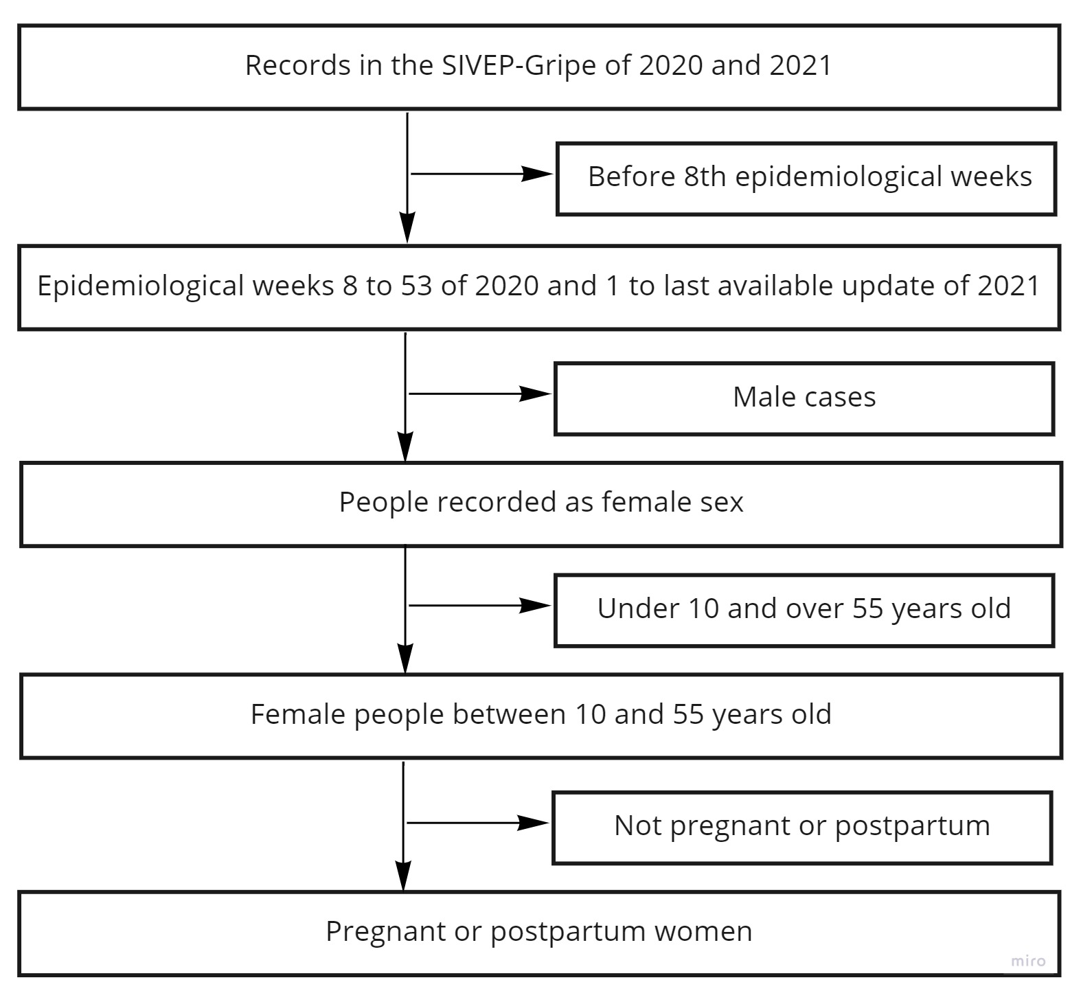
The two databases are merged and data are filtered from the 8th epidemiological week of symptoms (when the first confirmed case of COVID-19 was found in the database) to until the last available update of 2021. All data on female cases aged 10 to 55 years old, with information on whether pregnant women (first, second or third gestational period or with ignored gestational age) or in the puerperium period were included. The flowchart is shown in Figure 1.
The variables analyzed and available in OOBr COVID-19 are: age, race, education, state of Brazil of residence, region of Brazil of residence, age range, obstetric status, change of municipality for assistance, residence area, SARI diagnosis, laboratory (etiological) diagnosis, flu syndrome that progresses to SARI, type of antiviral, previous vaccination for influenza, hospital-acquired infection, travel history, contact with swine, signs and symptoms (fever, cough, sore throat, dyspnoea, respiratory distress, O2 saturation less than 95%, diarrhea, vomiting, abdominal pain, fatigue, loss of smell or taste), risk factors/comorbidities (cardiovascular disease, kidney disease, neurological disease, hematological disease, liver disease, diabetes, asthma, pneumopathy, obesity and immunosuppression), hospitalization, admission to the ICU (Intensive Care Unit), use of ventilatory support (invasive and non-invasive) and evolution of the case (cure or death).
3. Results
The analyzes that result in observatory https://observatorioobstetrico.shinyapps.io/covid_gesta_puerp_br are described in this section. At first, the R packages used are presented, the data are loaded, the selections and filters are made and, finally, the characterization variables, symptoms, comorbidities, and outcome variables are processed.
3.1 Database load and R packages used
The R packages used for filtering and data processing are presented in this subsection.
#R packages used
loadlibrary <- function(x) {
if (!require(x, character.only = TRUE)) {
install.packages(x, dependencies = T)
if (!require(x, character.only = TRUE))
stop("Package not found")
}
}
packages <-
c(
"readr",
"readxl",
"janitor",
"dplyr",
"forcats",
"stringr",
"lubridate",
"summarytools",
"magrittr",
"questionr",
"knitr"
)
lapply(packages, loadlibrary)
The 2020 and 2021 databases are loaded and they are also merged. Below are the databases updated on April 26, 2021, the last update available at the time of writing this article.
######### Importing databases
#2021
dados_2021 <- read_delim(
"INFLUD21-26-04-2021.csv",
";",
escape_double = FALSE,
locale = locale(encoding = "ISO-8859-2"),
trim_ws = TRUE
)
#2020
dados_2020 <- read_delim(
"INFLUD-26-04-2021.csv",
";",
escape_double = FALSE,
locale = locale(encoding = "ISO-8859-2"),
trim_ws = TRUE
)
####### Merging 2020 and 2021 databases
dados1 <- rbind(dados_2020, dados_2021)
3.2 Selecting cases and data processing
We will filter only the cases from the 8th epidemiological week of 2020 (first confirmed case of COVID-19) until the current epidemiological week of 2021.
#### Current epidemiological week
sem <- 16
#### Create year variable (ano)
dados1 <- dados1 %>%
dplyr::mutate(
dt_sint = as.Date(DT_SIN_PRI, format = "%d/%m/%Y"),
ano = lubridate::year(dt_sint),
)
#### Case filtering from the 8th epidemiological week of 2020
dados2 <- dados1 %>%
filter((ano==2020 & SEM_PRI >=8) | ano ==2021)
The table in the following presents the distribution of cases by year and by epidemiological week.
#### Cross table of epidemiological year and week
ctable(dados2$SEM_PRI, dados2$ano, prop="n")
## Cross-Tabulation
## SEM_PRI * ano
## Data Frame: dados2
##
## --------- ----- --------- -------- ---------
##             ano      2020     2021     Total
##   SEM_PRI
##         1               0    35122     35122
##         2               0    33809     33809
##         3               0    31044     31044
##         4               0    28985     28985
##         5               0    34670     34670
##         6               0    37745     37745
##         7               0    47328     47328
##         8             923    50091     51014
##         9            1164    68575     69739
##        10            1980    68057     70037
##        11            5136    65397     70533
##        12           12826    50657     63483
##        13           14974    45334     60308
##        14           16289    37006     53295
##        15           19583    19824     39407
##        16           24872     4445     29317
##        17           30828       19     30847
##        18           34864        0     34864
##        19           34566        0     34566
##        20           37172        0     37172
##        21           33824        0     33824
##        22           31256        0     31256
##        23           35643        0     35643
##        24           34162        0     34162
##        25           36694        0     36694
##        26           32968        0     32968
##        27           37444        0     37444
##        28           37041        0     37041
##        29           34440        0     34440
##        30           33704        0     33704
##        31           32184        0     32184
##        32           30028        0     30028
##        33           31070        0     31070
##        34           28271        0     28271
##        35           26337        0     26337
##        36           26459        0     26459
##        37           24047        0     24047
##        38           22222        0     22222
##        39           21579        0     21579
##        40           22451        0     22451
##        41           21026        0     21026
##        42           18999        0     18999
##        43           19464        0     19464
##        44           18719        0     18719
##        45           23302        0     23302
##        46           25802        0     25802
##        47           29289        0     29289
##        48           29162        0     29162
##        49           32940        0     32940
##        50           30540        0     30540
##        51           28405        0     28405
##        52           30304        0     30304
##        53           21559    12514     34073
##     Total         1176512   670622   1847134
## --------- ----- --------- -------- ---------
Note that there are 12514 cases in 2021 in week 53. These are cases from the first two days of 2021, which are still part of of the last epidemiological week of 2020 (http://portalsinan.saude.gov.br/calendario-epidemiologico?layout=edit&id=168). However, these cases belong to the 53rd week of 2020 and we corrected in the following:
#### Correcting year variable (ano) from 53rd epidemiological week
dados2 <- dados2 %>%
mutate(ano = ifelse(ano ==2021 & SEM_PRI ==53, 2020, ano)) %>%
filter(ano==2020 | (ano == 2021 & SEM_PRI <= sem))
The distribution of epidemiological week by year of the pandemic after correction is presented in the following.
#### Cross table of epidemiological year and week
ctable(dados2$SEM_PRI, dados2$ano, prop="n")
## Cross-Tabulation
## SEM_PRI * ano
## Data Frame: dados2
##
## --------- ----- --------- -------- ---------
##             ano      2020     2021     Total
##   SEM_PRI
##         1               0    35122     35122
##         2               0    33809     33809
##         3               0    31044     31044
##         4               0    28985     28985
##         5               0    34670     34670
##         6               0    37745     37745
##         7               0    47328     47328
##         8             923    50091     51014
##         9            1164    68575     69739
##        10            1980    68057     70037
##        11            5136    65397     70533
##        12           12826    50657     63483
##        13           14974    45334     60308
##        14           16289    37006     53295
##        15           19583    19824     39407
##        16           24872     4445     29317
##        17           30828        0     30828
##        18           34864        0     34864
##        19           34566        0     34566
##        20           37172        0     37172
##        21           33824        0     33824
##        22           31256        0     31256
##        23           35643        0     35643
##        24           34162        0     34162
##        25           36694        0     36694
##        26           32968        0     32968
##        27           37444        0     37444
##        28           37041        0     37041
##        29           34440        0     34440
##        30           33704        0     33704
##        31           32184        0     32184
##        32           30028        0     30028
##        33           31070        0     31070
##        34           28271        0     28271
##        35           26337        0     26337
##        36           26459        0     26459
##        37           24047        0     24047
##        38           22222        0     22222
##        39           21579        0     21579
##        40           22451        0     22451
##        41           21026        0     21026
##        42           18999        0     18999
##        43           19464        0     19464
##        44           18719        0     18719
##        45           23302        0     23302
##        46           25802        0     25802
##        47           29289        0     29289
##        48           29162        0     29162
##        49           32940        0     32940
##        50           30540        0     30540
##        51           28405        0     28405
##        52           30304        0     30304
##        53           34073        0     34073
##     Total         1189026   658089   1847115
## --------- ----- --------- -------- ---------
The next step is to identify pregnant women. For this, we will analyze the variable CS_GESTANT. This variable assumes the values: 1-1st trimester; 2-2nd trimester; 3-3rd trimester; 4-Ignored Gestational Age; 5-No; 6-Does not apply; 9-Ignored.
##### Frequency table for gestational information
questionr::freq(
dados2$CS_GESTANT,
cum = FALSE,
total = TRUE,
na.last = FALSE,
valid = FALSE
) %>%
kable(caption = "Frequency table for variable
about pregnancy", digits = 2)
| n | % | |
|---|---|---|
| 0 | 371 | 0.0 |
| 1 | 1938 | 0.1 |
| 2 | 4475 | 0.2 |
| 3 | 9593 | 0.5 |
| 4 | 978 | 0.1 |
| 5 | 574545 | 31.1 |
| 6 | 1163859 | 63.0 |
| 9 | 91356 | 4.9 |
| Total | 1847115 | 100.0 |
There are 371 cases with CS_GESTANT=0, where category 0 has no code in the database dictionary.
The next step is to check if there is any inconsistency when analyzing this variable together with sex (CS_SEXO), with categories F-female, M-male and I-ignored.
#### Cross table of gestation and sex
ctable(dados2$CS_GESTANT, dados2$CS_SEXO, prop="n")
## Cross-Tabulation
## CS_GESTANT * CS_SEXO
## Data Frame: dados2
##
## ------------ --------- -------- ----- -------- ---------
##                CS_SEXO        F     I        M     Total
##   CS_GESTANT
##            0                115   177       79       371
##            1               1938     0        0      1938
##            2               4474     1        0      4475
##            3               9592     1        0      9593
##            4                977     1        0       978
##            5             573354    51     1140    574545
##            6             165319   279   998261   1163859
##            9              91108    94      154     91356
##        Total             846877   604   999634   1847115
## ------------ --------- -------- ----- -------- ---------
There are 0 cases of CS_SEXO=M with CS_GESTANT=1,2,3 ou 4, hopefully.
The puerperium indicator variable is PUERPERA, with categories 1-yes, 2-no and 9-Ignored.
#Frequency table for puerperium
questionr::freq(
dados2$PUERPERA,
cum = FALSE,
total = TRUE,
na.last = FALSE,
valid = FALSE
) %>%
kable(caption = "Frequency table for puerperium", digits = 2)
| n | % | |
|---|---|---|
| 1 | 6648 | 0.4 |
| 2 | 682995 | 37.0 |
| 9 | 18082 | 1.0 |
| NA | 1139390 | 61.7 |
| Total | 1847115 | 100.0 |
The next step is to check if there is any inconsistency when analyzing this variable together with sex (CS_SEXO), with categories F-female, M-male and I-ignored.
#### Cross table of puerperium and sex
ctable(dados2$PUERPERA, dados2$CS_SEXO, prop="n")
## Cross-Tabulation
## PUERPERA * CS_SEXO
## Data Frame: dados2
##
## ---------- --------- -------- ----- -------- ---------
##              CS_SEXO        F     I        M     Total
##   PUERPERA
##          1               6647     1        0      6648
##          2             327159   174   355662    682995
##          9               8345    10     9727     18082
##       <NA>             504726   419   634245   1139390
##      Total             846877   604   999634   1847115
## ---------- --------- -------- ----- -------- ---------
There are 0 cases of CS_SEXO=M with PUERPERA = 1, that is, puerperium and male sex cases, hopefully.
The next selection is to consider only female people and aged over 10 and under or equal to 55 years.
#### Filtering only female cases
dados3 <- dados2 %>%
filter(CS_SEXO == "F")
#### Filtering of cases aged 55 years or less
dados4 <- dados3 %>%
filter(NU_IDADE_N > 9 & NU_IDADE_N <= 55)
Now we are going to create the variable of gestational trimester or puerperium. Note that for puerperium (puerp), nonpregnant or ignored cases with PUERPERA = 1 are considered.
#### Creation of the classi_gesta_puerp variable for the gestational or postpartum period
dados4 <- dados4 %>%
mutate(
classi_gesta_puerp = case_when(
CS_GESTANT == 1 ~ "1tri", # 1st trimester
CS_GESTANT == 2 ~ "2tri", # 2nd trimester
CS_GESTANT == 3 ~ "3tri", # 3rd trimester
CS_GESTANT == 4 ~ "IG_ig", # Ignored gestational age
CS_GESTANT == 5 &
PUERPERA == 1 ~ "puerp", # puerperal woman
CS_GESTANT == 9 & PUERPERA == 1 ~ "puerp", # puerperal woman
TRUE ~ "não" # ’não’ means not pregnant
)
)
The last filtering consists of selecting the cases of pregnant or postpartum women.
### Selection only of pregnant or postpartum cases
dados5 <- dados4 %>%
filter(classi_gesta_puerp != "não")
### Frequency table for gestational group
questionr::freq(
dados5$classi_gesta_puerp,
cum = FALSE,
total = TRUE,
na.last = FALSE,
valid = FALSE
) %>%
kable(caption = "Frequency table for gestational trimester or postpartum variable",
digits = 2)
| n | % | |
|---|---|---|
| 1tri | 1914 | 8.9 |
| 2tri | 4407 | 20.5 |
| 3tri | 9575 | 44.6 |
| IG_ig | 917 | 4.3 |
| puerp | 4661 | 21.7 |
| Total | 21474 | 100.0 |
In the following, we deal with other variables considered at the OOBr Covid-19.
3.3 Variables processing
The variable that indicates the SARI diagnosis is CLASSI_FIN, with categories: 1-SARI by influenza, 2-SARI by another respiratory virus, 3-SARI by another etiologic agent, 4-SARI not specified, 5-SARI by COVID-19.
#frequency table for SARI diagnosis
questionr::freq(
dados5$CLASSI_FIN,
cum = FALSE,
total = TRUE,
na.last = FALSE,
valid = FALSE
) %>%
kable(caption = "Frequency table for SARI diagnosis", digits = 2)
| n | % | |
|---|---|---|
| 1 | 74 | 0.3 |
| 2 | 105 | 0.5 |
| 3 | 61 | 0.3 |
| 4 | 8104 | 37.7 |
| 5 | 10818 | 50.4 |
| NA | 2312 | 10.8 |
| Total | 21474 | 100.0 |
The variable that identify the diagnostic type of COVID-19 is classi_covid, with categories: pcr (RT-PCR), antigenio (antigen), sorologia (serology) and outro (other). This variable only has valid categories for cases confirmed by SARI by COVID-19 (CLASSI_FIN=5).
#Case diagnosed by RT-PCR
dados5 <- dados5 %>%
mutate(pcr_SN = case_when(
(PCR_SARS2 == 1) |
(
str_detect(DS_PCR_OUT, "SARS|COVID|COV|CORONA|CIVID")
) ~ "sim",
TRUE ~ "não"
))
#Identify if diagnosed by serology
dados5$res_igg <-
ifelse(is.na(dados5$RES_IGG) == TRUE, 0, dados5$RES_IGG)
dados5$res_igm <-
ifelse(is.na(dados5$RES_IGM) == TRUE, 0, dados5$RES_IGM)
dados5$res_iga <-
ifelse(is.na(dados5$RES_IGA) == TRUE, 0, dados5$RES_IGA)
dados5$sorologia_SN <-
ifelse(dados5$res_igg == 1 |
dados5$res_igm == 1 | dados5$res_iga == 1,
"sim",
"não")
#Identify if diagnosed by antigen
dados5 <- dados5 %>%
mutate(antigeno_SN = case_when(
(AN_SARS2 == 1) | #positivo
(
str_detect(DS_AN_OUT, "SARS|COVID|COV|CORONA|CONA")
) ~ "sim",
TRUE ~ "não"
))
#Creation of the covid-19 classification variable
dados5 <- dados5 %>%
mutate(
classi_covid = case_when(
CLASSI_FIN == 5 & pcr_SN == "sim" ~ "pcr",
CLASSI_FIN == 5 & pcr_SN == "não" &
antigeno_SN == "sim" ~ "antigenio",
CLASSI_FIN == 5 & sorologia_SN == "sim" &
antigeno_SN == "não" &
pcr_SN == "não" ~ "sorologia",
CLASSI_FIN != 5 ~ "não", #is not another etiologic agent or unspecified
TRUE ~ "outro"
)
)
#frequency table for COVID-19 diagnostic type
questionr::freq(
dados5$classi_covid,
cum = FALSE,
total = TRUE,
na.last = FALSE,
valid = FALSE
) %>%
kable(caption = "Frequency table for the COVID-19 diagnostic type", digits = 2)
| n | % | |
|---|---|---|
| antigenio | 827 | 3.9 |
| não | 8344 | 38.9 |
| outro | 4354 | 20.3 |
| pcr | 6908 | 32.2 |
| sorologia | 1041 | 4.8 |
| Total | 21474 | 100.0 |
The variable that indicates the state of Brazil is SG_UF. The variable that indicates the region of Brazil (North, Northeast, Central, Southeast and South) is region, created in the following.
#Creation of the region variable
regions <- function(state) {
southeast <- c("SP", "RJ", "ES", "MG")
south <- c("PR", "SC", "RS")
central <- c("GO", "MT", "MS", "DF")
northeast <-
c("AL", "BA", "CE", "MA", "PB", "PE", "PI", "RN", "SE")
north <- c("AC", "AP", "AM", "PA", "RO", "RR", "TO")
out <-
ifelse(any(state == southeast),
"southeast",
ifelse(any(state == south),
"south",
ifelse(
any(state == central),
"central",
ifelse(any(state == northeast),
"northeast", "north")
)))
return(out)
}
dados5$region <- sapply(dados5$SG_UF, regions)
dados5$region <-
ifelse(is.na(dados5$region) == TRUE, 0, dados5$region)
#Frequency table for region
questionr::freq(
dados5$region,
cum = FALSE,
total = TRUE,
na.last = FALSE,
valid = FALSE
) %>%
kable(caption = "Frequency table for the region of Brazil", digits = 2)
| n | % | |
|---|---|---|
| 0 | 4 | 0.0 |
| central | 2384 | 11.1 |
| north | 2363 | 11.0 |
| northeast | 5394 | 25.1 |
| south | 2671 | 12.4 |
| southeast | 8658 | 40.3 |
| Total | 21474 | 100.0 |
Note that there are 4 cases without information for the region of the country (encoded as 0).
The processing of the characterization variables is presented in the following.
#Race
dados5 <- dados5 %>%
mutate(
raca = case_when(
CS_RACA == 1 ~ "branca", #white
CS_RACA == 2 ~ "preta", #black
CS_RACA == 3 ~ "amarela", #yellow
CS_RACA == 4 ~ "parda", #brown
CS_RACA == 5 ~ "indigena", #indigenous
TRUE ~ NA_character_
)
)
#Education
dados5 <- dados5 %>%
mutate(
escol = case_when(
CS_ESCOL_N == 0 ~ "sem escol", #no school
CS_ESCOL_N == 1 ~ "fund1", #1st elementary school
CS_ESCOL_N == 2 ~ "fund2", #2nd elementary school
CS_ESCOL_N == 3 ~ "medio", #high school
CS_ESCOL_N == 4 ~ "superior", #university education
TRUE ~ NA_character_
)
)
#Age range
dados5 <- dados5 %>%
mutate(
faixa_et = case_when(
NU_IDADE_N <= 19 ~ "<20",
NU_IDADE_N >= 20
& NU_IDADE_N <= 34 ~ "20-34",
NU_IDADE_N >= 35 ~ ">=35",
TRUE ~ NA_character_
)
)
dados5$faixa_et <-
factor(dados5$faixa_et, levels = c("<20", "20-34", ">=35"))
#Hospitalization
dados5 <- dados5 %>%
mutate(hospital = case_when(HOSPITAL == 1 ~ "sim", #yes
HOSPITAL == 2 ~ "não", #no
TRUE ~ NA_character_))
#Travel history
dados5 <- dados5 %>%
mutate(hist_viagem = case_when(HISTO_VGM == 1 ~ "sim", #yes
HISTO_VGM == 2 ~ "não", #no
TRUE ~ NA_character_))
#Influenza syndrome evolved to SARI
dados5 <- dados5 %>%
mutate(sg_para_srag = case_when(SURTO_SG == 1 ~ "sim", #yes
SURTO_SG == 2 ~ "não", #no
TRUE ~ NA_character_))
#Hospital acquired infection
dados5 <- dados5 %>%
mutate(inf_inter = case_when(NOSOCOMIAL == 1 ~ "sim", #yes
NOSOCOMIAL == 2 ~ "não", #no
TRUE ~ NA_character_))
#Contact with poultry or swine
dados5 <- dados5 %>%
mutate(cont_ave_suino = case_when(AVE_SUINO == 1 ~ "sim", #yes
AVE_SUINO == 2 ~ "não", #no
TRUE ~ NA_character_))
#Influenza vaccine
dados5 <- dados5 %>%
mutate(vacina = case_when(VACINA == 1 ~ "sim", #yes
VACINA == 2 ~ "não", #no
TRUE ~ NA_character_))
#Antiviral
dados5 <- dados5 %>%
mutate(
antiviral = case_when(
ANTIVIRAL == 1 ~ "Oseltamivir",
ANTIVIRAL == 2 ~ "Zanamivir",
TRUE ~ NA_character_ ))
#Residence zone
dados5 <- dados5 %>%
mutate(zona = case_when(CS_ZONA == 1 ~ "urbana", #urban
CS_ZONA == 2 ~ "rural", #rural
CS_ZONA == 3 ~ "periurbana", #periurban
TRUE ~ NA_character_))
#If change of municipality for care
dados5 <- dados5 %>%
mutate(mudou_muni = case_when(CO_MUN_RES==CO_MU_INTE & !is.na(CO_MU_INTE) &
!is.na(CO_MUN_RES) ~ "não", #no
CO_MUN_RES!=CO_MU_INTE & !is.na(CO_MU_INTE) &
!is.na(CO_MUN_RES) ~ "sim", #yes
TRUE ~ NA_character_
)
)
The processing of symptom variables is presented below.
#Fever
dados5 <- dados5 %>%
mutate(febre = case_when(FEBRE == 1 ~ "sim", #yes
FEBRE == 2 ~ "não", #no
TRUE ~ NA_character_))
#Cough
dados5 <- dados5 %>%
mutate(tosse = case_when(TOSSE == 1 ~ "sim", #yes
TOSSE == 2 ~ "não", #no
TRUE ~ NA_character_))
#Sore throat
dados5 <- dados5 %>%
mutate(garganta = case_when(GARGANTA == 1 ~ "sim", #yes
GARGANTA == 2 ~ "não", #no
TRUE ~ NA_character_))
#Dyspnea
dados5 <- dados5 %>%
mutate(dispneia = case_when(DISPNEIA == 1 ~ "sim", #yes
DISPNEIA == 2 ~ "não", #no
TRUE ~ NA_character_))
#Respiratory distress
dados5 <- dados5 %>%
mutate(desc_resp = case_when(DESC_RESP == 1 ~ "sim", #yes
DESC_RESP == 2 ~ "não", #no
TRUE ~ NA_character_))
#O2 saturation less than 95%
dados5 <- dados5 %>%
mutate(saturacao = case_when(SATURACAO == 1 ~ "sim", #yes
SATURACAO == 2 ~ "não", #no
TRUE ~ NA_character_))
#Diarrhea
dados5 <- dados5 %>%
mutate(diarreia = case_when(DIARREIA == 1 ~ "sim", #yes
DIARREIA == 2 ~ "não", #no
TRUE ~ NA_character_))
#Vomiting
dados5 <- dados5 %>%
mutate(vomito = case_when(VOMITO == 1 ~ "sim", #yes
VOMITO == 2 ~ "não", #no
TRUE ~ NA_character_))
#Abdominal pain
dados5 <- dados5 %>%
mutate(dor_abd = case_when(DOR_ABD == 1 ~ "sim",
DOR_ABD == 2 ~ "não",
TRUE ~ NA_character_))
#Fatigue
dados5 <- dados5 %>%
mutate(fadiga = case_when(FADIGA == 1 ~ "sim", #yes
FADIGA == 2 ~ "não", #no
TRUE ~ NA_character_))
#Olfactory loss
dados5 <- dados5 %>%
mutate(perd_olft = case_when(PERD_OLFT == 1 ~ "sim", #yes
PERD_OLFT == 2 ~ "não", #no
TRUE ~ NA_character_))
#Loss of taste
dados5 <- dados5 %>%
mutate(perd_pala = case_when(PERD_PALA == 1 ~ "sim", #yes
PERD_PALA == 2 ~ "não", #no
TRUE ~ NA_character_))
The processing of comorbidity variables is presented below.
#Cardiovascular disease
dados5 <- dados5 %>%
mutate(cardiopati = case_when(CARDIOPATI == 1 ~ "sim", #yes
CARDIOPATI == 2 ~ "não", #no
TRUE ~ NA_character_))
#Hematological disease
dados5 <- dados5 %>%
mutate(hematologi = case_when(HEMATOLOGI == 1 ~ "sim", #yes
HEMATOLOGI == 2 ~ "não", #no
TRUE ~ NA_character_))
#Liver disease
dados5 <- dados5 %>%
mutate(hepatica = case_when(HEPATICA == 1 ~ "sim", #yes
HEPATICA == 2 ~ "não", #no
TRUE ~ NA_character_))
#Asthma
dados5 <- dados5 %>%
mutate(asma = case_when(ASMA == 1 ~ "sim", #yes
ASMA == 2 ~ "não", #no
TRUE ~ NA_character_))
#Diabetes
dados5 <- dados5 %>%
mutate(diabetes = case_when(DIABETES == 1 ~ "sim", #yes
DIABETES == 2 ~ "não", #no
TRUE ~ NA_character_))
#Neurological disease
dados5 <- dados5 %>%
mutate(neuro = case_when(NEUROLOGIC == 1 ~ "sim", #yes
NEUROLOGIC == 2 ~ "não", #no
TRUE ~ NA_character_))
#Pneumopathy
dados5 <- dados5 %>%
mutate(pneumopati = case_when(PNEUMOPATI == 1 ~ "sim", #yes
PNEUMOPATI == 2 ~ "não", #no
TRUE ~ NA_character_))
#Immunosuppression
dados5 <- dados5 %>%
mutate(imunodepre = case_when(IMUNODEPRE == 1 ~ "sim", #yes
IMUNODEPRE == 2 ~ "não", #no
TRUE ~ NA_character_))
#Kidney disease
dados5 <- dados5 %>%
mutate(renal = case_when(RENAL == 1 ~ "sim", #yes
RENAL == 2 ~ "não", #no
TRUE ~ NA_character_))
#Obesity
dados5 <- dados5 %>%
mutate(obesidade = case_when(OBESIDADE == 1 ~ "sim", #yes
OBESIDADE == 2 ~ "não", #no
TRUE ~ NA_character_))
The processing of the variables admission to the ICU, use of ventilatory support and evolution (death or cure) is done as follows
#ICU
dados5 <- dados5 %>%
mutate(uti = case_when(UTI == 1 ~ "sim", #yes
UTI == 2 ~ "não", #no
TRUE ~ NA_character_))
#Use of ventilatory support
dados5 <- dados5 %>%
mutate(
suport_ven = case_when(
SUPORT_VEN == 1 ~ "invasivo", #invasive
SUPORT_VEN == 2 ~ "não invasivo", #non-invasive
SUPORT_VEN == 3 ~ "não", #no
TRUE ~ NA_character_
)
)
dados5$suport_ven <- factor(dados5$suport_ven,
levels = c("invasivo", "não invasivo", "não"))
#Evolution
dados5 <-
dados5 %>% mutate(
evolucao = case_when(
EVOLUCAO == 1 ~ "Cura", #cure
EVOLUCAO == 2 ~ "Obito", #death
EVOLUCAO == 3 ~ "Obito", #death
TRUE ~ NA_character_
)
)
The analyzes obtained after the processes described above are presented in https://observatorioobstetrico.shinyapps.io/covid_gesta_puerp_br.
4. Final remarks
In this article we present the documentation for loading the data, merge data from the years 2020 and 2021, selection and filtering cases and processing the variables to obtain the analyzes in OOBr COVID-19, available in https://observatorioobstetrico.shinyapps.io/covid_gesta_puerp_br.
With OOBr COVID-19 we hope that information about COVID-19 in the Brazilian maternal population will be accessible so that society is aware of the pandemic situation in the country and that public policy decisions are based on reliable data.
Funding
OOBr is financed by the Bill & Melinda Gates Foundation, CNPq (National Council for Scientific and Technological Development), DECIT/MS (Department of Science and Technology of the Ministry of Health of Brazil) and FAPES (Espírito Santo Research and Innovation Support Foundation).
References
[1] Zambrano LD, Ellington S, Strid P, Galang RR, Oduyebo T, Tong VT, Woodworth KR, Nahabedian JF 3rd, Azziz-Baumgartner E, Gilboa SM, Meaney-Delman D; CDC COVID-19 Response Pregnancy and Infant Linked Outcomes Team. Update: Characteristics of Symptomatic Women of Reproductive Age with Laboratory-Confirmed SARS-CoV-2 Infection by Pregnancy Status - United States, January 22-October 3, 2020. MMWR Morb Mortal Wkly Rep. 2020 Nov 6;69(44):1641-1647. doi: 10.15585/mmwr.mm6944e3. PMID: 33151921; PMCID: PMC7643892
[2] Brasil. Ministério da Saúde. Departamento de informática. [Open data SUS System] [Internet].
https://opendatasus.saude.gov.br/dataset/bd-srag-2020, accessed April 26, 2021.
[3] Brasil. Ministério da Saúde. Departamento de informática. [Open data SUS System] [Internet].
https://opendatasus.saude.gov.br/dataset/bd-srag-2021, accessed April 26, 2021.