Quantum fluxes at the inner horizon of a near-extremal spherical charged black hole

Abstract

We analyze and compute the semiclassical stress-energy flux components, the outflux $\left\langle T_{uu}\right\rangle_{\text{ren}}$ and the influx $\left\langle T_{vv}\right\rangle_{\text{ren}}$ ($u$ and $v$ being the standard null Eddington coordinates), at the inner horizon (IH) of a Reissner-Nordström black hole (BH) of mass $M$ and charge $Q$, in the near-extremal domain in which $Q/M$ approaches $1$. We consider a minimally-coupled massless quantum scalar field, in both Hartle-Hawking and Unruh states, the latter corresponding to an evaporating BH. The near-extremal domain lends itself to an analytical treatment which sheds light on the behavior of various quantities on approaching extremality. We explore the behavior of the three near-IH flux quantities $\left\langle T_{uu}^{-}\right\rangle_{\text{ren}}^{U}$, $\left\langle T_{vv}^{-}\right\rangle_{\text{ren}}^{U}$, and $\left\langle T_{uu}^{-}\right\rangle_{\text{ren}}^{H}=\left\langle T_{vv}^{-}\right\rangle_{\text{ren}}^{H}$, as a function of the small parameter $\Delta\equiv\sqrt{1-\left(Q/M\right)^{2}}$ (where the superscript “$U$” or “$H$” respectively refers to the Unruh or Hartle-Hawking state and “$-$” refers to the IH value). We find that in the near-extremal domain $\left\langle T_{uu}^{-}\right\rangle_{\text{ren}}^{U}\cong\left\langle T_{uu}^{-}\right\rangle_{\text{ren}}^{H}=\left\langle T_{vv}^{-}\right\rangle_{\text{ren}}^{H}$ behaves as $\propto\Delta^{5}$. In contrast, $\left\langle T_{vv}^{-}\right\rangle_{\text{ren}}^{U}$ behaves as $\propto\Delta^{4}$, and we calculate the prefactor analytically. It therefore follows that the semiclassical fluxes at the IH neighborhood of an evaporating near-extremal spherical charged BH are dominated by the influx $\left\langle T_{vv}\right\rangle_{\text{ren}}^{U}$.

In passing, we also find an analytical expression for the transmission coefficient outside a Reissner-Nordström BH to leading order in small frequencies (which turns out to be a crucial ingredient of our near-extremal analysis). Furthermore, we explicitly obtain the near-extremal Hawking-evaporation rate ($\propto\Delta^{4}$), with an analytical expression for the prefactor (obtained here for the first time to the best of our knowledge).

I Introduction.

This paper extends our previous one (FluxesIH:2020, ), in which we computed and investigated the semiclassical stress-energy fluxes at the inner horizon (IH) of a spherical charged black hole (BH). Whereas in the previous paper we considered BHs with a broad range of $Q/M$ values, here we restrict our attention to the near-extremal limit where $Q/M$ approaches unity, where $Q$ and $M$ respectively denote the BH’s charge and mass.

The semiclassical formulation of general relativity treats matter fields as quantum fields, propagating on a spacetime background described by a classical metric $g_{\alpha\beta}(x^{\mu})$. The classical Einstein field equation is then replaced by its semiclassical counterpart:

$$G_{\alpha\beta}=8\pi\left\langle T_{\alpha\beta}\right\rangle_{\text{ren}}$$

where $G_{\alpha\beta}$ is the Einstein tensor associated with $g_{\alpha\beta}$ and $\left\langle T_{\alpha\beta}\right\rangle_{\text{ren}}$ is the renormalized expectation value of the stress-energy tensor (RSET) associated with the quantum field in consideration. Evidently, the quantum field and the geometry of spacetime undergo mutual influence. In particular, the curved geometry of spacetime induces a non-trivial stress-energy tensor, even in vacuum states, which in turn deforms the underlying background geometry — a phenomenon known as backreaction.

As our spacetime background, we hereby consider a spherical charged BH given in the standard Schwarzschild coordinates by the Reissner-Nordström (RN) metric,

$$\text{d}s^{2}=-f\left(r\right)\text{d}t^{2}+f^{-1}\left(r\right)\text{d}r^{2}+r^{2}\left(\text{d}\theta^{2}+\sin^{2}\theta\text{d}\phi^{2}\right)\,,$$

with the $r$-dependent function $f\left(r\right)=1-\frac{2M}{r}+\frac{Q^{2}}{r^{2}}$. We consider a non-extremal RN BH, meaning $0<Q/M<1$ . This BH metric admits two horizons, corresponding to the two real roots of $f\left(r\right)$, denoted by $r_{\pm}=M\pm\sqrt{M^{2}-Q^{2}}$; the event horizon (EH) is located at $r=r_{+}$, while the IH is located at $r=r_{-}$. For later use, we also define the two surface gravity parameters, $\kappa_{\pm}=\left(r_{+}-r_{-}\right)/2r_{\pm}^{2}$.

Upon this BH background we introduce an (uncharged) minimally-coupled massless scalar field $\Phi$, evolving according to the Klein-Gordon equation

$$\square\Phi=0\,,$$

with $\square$ the covariant d’Alembertian associated with the RN metric. This field may be decomposed into standard $\omega lm$ modes, which, due to the RN metric symmetries, can be factorized into a $t$-dependent term $e^{-i\omega t}$, an angular term $Y_{lm}\left(\theta,\phi\right)$, and a term that depends on $r$ alone. We cast this last term as $\psi_{\omega l}\left(r\right)/r$, where $\psi_{\omega l}\left(r\right)$ is the so-called radial function obeying the radial equation:

$$\frac{\text{d}^{2}\psi_{\omega l}\left(r\right)}{\text{d}r_{*}^{2}}=\left[V_{l}\left(r\right)-\omega^{2}\right]\psi_{lm}\left(r\right)\,,$$ (I.1)

where the $r$-dependent effective potential $V_{l}\left(r\right)$ is given by

$$V_{l}\left(r\right)=f\left(r\right)\left[\frac{l\left(l+1\right)}{r^{2}}+\frac{\text{d}f/\text{d}r}{r}\right]\,,$$ (I.2)

and $r_{*}$ is the tortoise coordinate defined through $\text{d}r/\text{d}r_{*}=f\left(r\right)$.

We shall consider our field in two vacuum quantum states: the Hartle-Hawking (HH) state (HH:1976, ; Israel:1976, ), corresponding to a quantum field in thermal equilibrium with an infinite bath of radiation, and the more physically feasible Unruh state (Unruh:1976, ), describing the quantum state of a BH that evaporates via Hawking radiation.

We introduce the future-directed null Eddington coordinates, given inside the BH by $u=r_{*}-t$ and $v=r_{*}+t$. The $\left\langle T_{uu}\right\rangle_{\text{ren}}$ and $\left\langle T_{vv}\right\rangle_{\text{ren}}$ components of the RSET are referred to as the flux components, as they may, for example, describe correspondingly an ingoing and an outgoing flux of radiation. In the HH state, time-inversion symmetry implies $\left\langle T_{uu}\left(r\right)\right\rangle_{\text{ren}}=\left\langle T_{vv}\left(r\right)\right\rangle_{\text{ren}}$. In both quantum states, energy-momentum conservation yields the constancy (namely $r$-independence) of the quantity

$$4\pi r^{2}\left\langle T_{t}^{r}\right\rangle_{\text{ren}}=4\pi r^{2}\left(\left\langle T_{uu}\right\rangle_{\text{ren}}-\left\langle T_{vv}\right\rangle_{\text{ren}}\right)\,.$$ (I.3)

In the HH state this constant trivially vanishes. In the Unruh state, it coincides with the Hawking outflux (as may be seen by evaluating the above expression at $r\to\infty$, noting that in the Unruh state $r^{2}\left\langle T_{vv}\right\rangle_{\text{ren}}$ vanishes in that limit).

As discussed in Ref. (FluxesIH:2020, ), the flux components are crucial for backreaction in the vicinity of the IH, potentially having an accumulating effect on the form of the metric there. We thus concentrate on the IH value of the three flux quantities, $\left\langle T_{uu}^{-}\right\rangle_{\text{ren}}^{H}$, $\left\langle T_{uu}^{-}\right\rangle_{\text{ren}}^{U}$ and $\left\langle T_{vv}^{-}\right\rangle_{\text{ren}}^{U}$, where the superscript ”$H$” (”$U$”) corresponds to the HH (Unruh) state, and an upper “$-$” indicates the IH limit. (Hereafter, the term flux quantities will refer to these three IH quantities.) In Ref. (FluxesIH:2020, ), we computed the near-IH flux components in both quantum states for a variety of non-extremal RN BHs, and displayed the results as a function of $Q/M$ (for a related work, see also Ref. (Hollands:2020, )). All three flux quantities, $\left\langle T_{uu}^{-}\right\rangle_{\text{ren}}^{H}$, $\left\langle T_{uu}^{-}\right\rangle_{\text{ren}}^{U}$ and $\left\langle T_{vv}^{-}\right\rangle_{\text{ren}}^{U}$, were found to change their sign at some $Q/M$ value (all around $\approx 0.967$), being increasingly positive at lower $Q/M$ values and becoming negative beyond that critical $Q/M$ value. Furthermore, as $Q/M$ grows towards the extremal value of $1$, all flux quantities decay to zero (at different rates).

Here, we intend to take a closer look at the near-extremal limit, characterized by $1-Q/M\ll 1$. That is, we wish to examine the near-IH fluxes as $Q/M$ approaches 1. As we shall see, the near-extremal domain lends itself to analytical investigation, which sheds light on the behavior we see numerically. In fact, we find it beneficial to focus on an equivalent set of three quantities, being the elementary flux quantity $\left\langle T_{uu}^{-}\right\rangle_{\text{ren}}^{H}$ and the differences $\left\langle T_{uu}^{-}\right\rangle_{\text{ren}}^{H}-\left\langle T_{uu}^{-}\right\rangle_{\text{ren}}^{U}$ and $\left\langle T_{uu}^{-}\right\rangle_{\text{ren}}^{U}-\left\langle T_{vv}^{-}\right\rangle_{\text{ren}}^{U}$ . The study of the differences, rather than the flux quantities directly, allows a sharper investigation of the near-extremal domain, as these differences vanish faster than their constituents on approaching extremality.

One obvious motivation to consider the near-extremal limit is the very evaporation process considered here: Since our scalar field $\Phi$ is uncharged, the BH charge remains fixed at all times, while the mass steadily shrinks due to the emission of Hawking radiation. In the long run, the BH mass $M$ will decay asymptotically to $Q$. As $M$ approaches $Q$, the Hawking temperature vanishes and the evaporation rate decays to zero. Note that in such an evaporation process the BH lasts forever, approaching extremality at the late-time limit (for a detailed discussion of this evaporation process, see Ref. (Jacobson, )).

To compute the quantum fluxes in the IH-vicinity, we shall employ the $\theta$-splitting variant (AAtheta:2016, ; LeviThetaRSET, ) of the “pragmatic mode-sum regularization” (PMR) method (AAt:2015, ; AARSET:2016, ; LeviRSET:2017, ), as we did in Ref. (FluxesIH:2020, ). Here, however, owing to the notable simplicity of the near-extremal limit, we shall carry this computation mostly analytically, and then validate our analytical results against numerical ones.

The rest of the paper is organized as follows. In Sec. II we develop the required preliminaries for the near-extremal analysis. Sec. III serves as the core of the paper, in which we perform the analysis of the flux quantities and their differences in the near-extremal limit. Numerical results and their agreement with the expressions found in the previous section are presented in Sec. IV. We end with a summary of our results and a short discussion in Sec. V. In the Appendix we analyze the transmission coefficient outside the BH to leading order in low frequencies, a quantity required for our analysis.

In this paper, we work in general-relativistic units $c=G=1$ and signature $(-+++)$.

II Preliminaries.

In this section we lay the foundations for the near-extremal analysis. The first subsection presents the basic expressions for the three flux quantities at the IH, as developed in Ref. (FluxesIH:2020, ), from which we construct the three quantities to be focused on in this paper. The second subsection is devoted to analyzing the internal radial function in the near-extremal limit, particularly in the vicinity of the IH.

II.1 Basic expressions for the fluxes and their differences at the IH.

In the BH interior, we endow the radial equation (I.1) with the initial condition of a free incoming wave at the EH :

$$\psi_{\omega l}\cong e^{-i\omega r_{*}}\,,\,\,\,\,\,\,r_{*}\to-\infty\,.$$ (II.1)

At the other edge, in the IH vicinity, the effective potential (I.2) vanishes like $r-r_{-}$ . Hence, the radial function (satisfying Eq. (I.1)) attains the general free asymptotic form:

$$\psi_{\omega l}\cong A_{\omega l}e^{i\omega r_{*}}+B_{\omega l}e^{-i\omega r_{*}}\,,\,\,\,\,\,\,r_{*}\to\infty$$ (II.2)

with $A_{\omega l}$ and $B_{\omega l}$ some constant coefficients determined by the scattering inside the BH. Notably, $A_{\omega l}$ and $B_{\omega l}$ satisfy the relation

$$\left|B_{\omega l}\right|^{2}-\left|A_{\omega l}\right|^{2}=1\,,$$ (II.3)

arising from the invariance of the Wronskian of $\psi_{\omega l}$ and its complex conjugate.

The basic quantities we concentrate on hereafter involve $A_{\omega l}$ and $B_{\omega l}$, as well as the transmission and reflection coefficients $\tau_{\omega l}^{\text{up}}$ and $\rho_{\omega l}^{\text{up}}$ for the “up” modes scattered outside the BH (see definition in Ref. (Group:2018, )). We shall analyze the near-extremal limit of $A_{\omega l}$ and $B_{\omega l}$ in Sec. II.2.1, while an analysis of $\tau_{\omega l}^{\text{up}}$ and $\rho_{\omega l}^{\text{up}}$ is deferred to the Appendix.

As mentioned in the introduction, we shall be interested in the flux components $\left\langle T_{uu}\right\rangle_{\text{ren}}$ and $\left\langle T_{vv}\right\rangle_{\text{ren}}$ in both quantum states, in the vicinity of the IH. In Ref. (FluxesIH:2020, ) we obtained expressions for these three elementary flux quantities, $\left\langle T_{uu}^{-}\right\rangle_{\text{ren}}^{H}$, $\left\langle T_{uu}^{-}\right\rangle_{\text{ren}}^{U}$ and $\left\langle T_{vv}^{-}\right\rangle_{\text{ren}}^{U}$, as a regularized mode sum, employing the $\theta$-splitting variant of the PMR method. We hereby quote the resulting expressions for convenience (see Eqs. (9)-(13) therein).

The flux quantities at the IH are generally given by

$$\left\langle T_{yy}^{-}\right\rangle_{\text{ren}}^{\Xi} =\hbar\sum_{l=0}^{\infty}\frac{2l+1}{8\pi}\left(F_{l\left(yy\right)}^{\Xi}-\beta\right)\,,$$ (II.4)

where the superscript “$\Xi$“ denotes the state (either $H$ or $U$), the subscript “$y$“ stands for either $u$ or $v$,

$$F_{l\left(yy\right)}^{\Xi}\equiv\int_{0}^{\infty}d\omega\,\hat{E}_{\omega l\left(yy\right)}^{\Xi}\,,$$

and $\beta$ is a constant (the so-called “blind-spot”; to be given explicitly in Eq. (II.8) below), which is the large-$l$ limit of $F_{l\left(yy\right)}^{\Xi}$. The integrand $\hat{E}_{\omega l\left(yy\right)}$ for the HH state is:

$$\hat{E}_{\omega l\left(yy\right)}^{H}=\frac{\omega}{\pi r_{-}^{2}}\left[\coth\left(\pi\omega/\kappa_{+}\right)\left|A_{\omega l}\right|^{2}+\text{csch}\left(\pi\omega/\kappa_{+}\right)\,\Re\left(\rho_{\omega l}^{\text{up}}A_{\omega l}B_{\omega l}\right)\right]\,$$ (II.5)

(where $\Re$ denotes the real part and $\text{csch}\equiv 1/\sinh$), and the corresponding integrands in the Unruh state are given by:

$$\hat{E}_{\omega l\left(uu\right)}^{U} =\hat{E}_{\omega l\left(yy\right)}^{H}+\frac{\omega}{2\pi r_{-}^{2}}\left[1-\coth\left(\pi\omega/\kappa_{+}\right)\right]\left|\tau_{\omega l}^{\text{up}}\right|^{2}\left|A_{\omega l}\right|^{2}\,,$$ (II.6)

$$\hat{E}_{\omega l\left(vv\right)}^{U} =\hat{E}_{\omega l\left(yy\right)}^{H}+\frac{\omega}{2\pi r_{-}^{2}}\left[1-\coth\left(\pi\omega/\kappa_{+}\right)\right]\left|\tau_{\omega l}^{\text{up}}\right|^{2}\left|B_{\omega l}\right|^{2}$$ (II.7)

Note that the difference between any of the two Unruh integrands and the HH integrand goes like $\propto\left|\tau_{\omega l}^{\text{up}}\right|^{2}$, which in turn decays with $l$ for fixed $\omega$ (note that the potential barrier outside the BH, given in Eq. (I.2), goes like $l\left(l+1\right)$, thus blocking the transmission at large $l$). Hence, all three flux quantities share the same large-$l$ “blind-spot” $\beta$, which may be analytically derived (see Sec. 3 in the Supplemental Material of Ref. (FluxesIH:2020, )) to be given by:

$$\beta=\frac{1}{24\pi r_{-}^{2}}\left(\kappa_{-}^{2}-\kappa_{+}^{2}\right)\,.$$ (II.8)

The three flux quantities $\left\langle T_{uu}^{-}\right\rangle_{\text{ren}}^{H}$, $\left\langle T_{uu}^{-}\right\rangle_{\text{ren}}^{U}$ and $\left\langle T_{vv}^{-}\right\rangle_{\text{ren}}^{U}$ (to which we shall hereafter also refer collectively as the elementary triplet) were the focus of our previous paper (FluxesIH:2020, ), where they were computed for a wide variety of subextremal $Q/M$ values. However, in the near-extremal domain, we find it worthwhile to organize these three flux quantities in a different manner. That is, we shall focus on an equivalent, slightly different, set of three quantities (to which we shall occasionally refer as the derived triplet): (i) the near-IH flux component in the HH state, $\left\langle T_{uu}^{-}\right\rangle_{\text{ren}}^{H}$, which also equals $\left\langle T_{vv}^{-}\right\rangle_{\text{ren}}^{H}$; (ii) the difference between the HH and Unruh values of $\left\langle T_{uu}^{-}\right\rangle_{\text{ren}}$, which we shall denote by $\left\langle T_{uu}^{-}\right\rangle_{\text{ren}}^{H-U}\equiv\left\langle T_{uu}^{-}\right\rangle_{\text{ren}}^{H}-\left\langle T_{uu}^{-}\right\rangle_{\text{ren}}^{U}$; and (iii) the difference between the two near-IH flux components in the Unruh state, multiplied by $4\pi r_{-}^{2}$, namely $\Lambda\equiv 4\pi r_{-}^{2}\left(\left\langle T_{uu}^{-}\right\rangle_{\text{ren}}^{U}-\left\langle T_{vv}^{-}\right\rangle_{\text{ren}}^{U}\right)$. Other than its interesting behavior in the near-extremal domain, considering $\Lambda$ has further motivation – one may recognize it as the conserved quantity mentioned in Eq. (I.3), in the Unruh state, evaluated at the IH. Obviously, since this quantity is independent of $r$, its value may also be evaluated outside the BH. In this sense, $\Lambda$ is the simplest quantity of all three members of the derived triplet, as it is fully determined by the scattering problem outside the BH.

The first quantity, $\left\langle T_{uu}^{-}\right\rangle_{\text{ren}}^{H}$, is given in Eqs. (II.4), (II.5) and (II.8). The second quantity $\left\langle T_{uu}^{-}\right\rangle_{\text{ren}}^{H-U}$ is determined from Eqs. (II.4) and (II.6), or explicitly:

$$\left\langle T_{uu}^{-}\right\rangle_{\text{ren}}^{H-U}=\hbar\sum_{l=0}^{\infty}\frac{2l+1}{4\pi}\int_{0}^{\infty}d\omega\,\frac{\omega}{4\pi r_{-}^{2}}\left[\coth\left(\pi\omega/\kappa_{+}\right)-1\right]\left|\tau_{\omega l}^{\text{up}}\right|^{2}\left|A_{\omega l}\right|^{2}\,.$$ (II.9)

Finally, the third quantity $\Lambda$ is obtained by subtracting Eq. (II.6) from Eq. (II.7) and using the Wronskian relation (II.3):

$$\Lambda=\hbar\sum_{l=0}^{\infty}\frac{2l+1}{4\pi}\int_{0}^{\infty}d\omega\,\omega\left[\coth\left(\pi\omega/\kappa_{+}\right)-1\right]\left|\tau_{\omega l}^{\text{up}}\right|^{2} \,.$$ (II.10)

As expected, this conserved quantity only requires the transmission coefficient outside the BH. Indeed, this is the known expression for the luminosity of an evaporating BH (see, for example, Eq. (136) in Ref. (DeWitt:1975, ) or Eq. (6.20) in Ref. (ChristensenFulling:1977, ) for the Schwarzschild case. The only modification needed is replacing the Schwarzschild $\kappa$ parameter by the corresponding RN parameter $\kappa_{+}$).

In Sec. III we shall take the above expressions for the derived triplet of quantities, which are valid for any $Q/M$, and evaluate them in the near-extremal domain of $Q/M$ approaching $1$.

II.2 The rescaled radial equation.

To quantify near-extremality, we define the dimensionless parameter $\Delta$ to be half the difference between $r_{+}/M$ and $r_{-}/M$:

$$\Delta\equiv\sqrt{1-\left(Q/M\right)^{2}}=r_{+}/M-1=1-r_{-}/M\,.$$ (II.11)

Note that $\Delta$ varies from $1$ (Schwarzschild) to $0$ (extremal RN), whereas the near-extremal domain is characterized by $\Delta\ll 1$. We shall examine the behavior of the various quantities upon approaching extremality by constructing their leading-order expansions in small $\Delta$.

To analyze the scaling with $\Delta$, it may be helpful to rewrite the radial equation (I.1) in a $\Delta$-normalized fashion, as we shall now demonstrate.

In the BH interior, the radial variable $r$ is confined to a domain of width $2M\Delta$,

$$1-\Delta\leq r/M\leq 1+\Delta\,.$$

That is, $r/M-1$ scales linearly with $\Delta$. We thus define the rescaled variable

$$s\equiv\frac{r/M-1}{\Delta}\,,$$

suitable for our near-extremal analysis. Note that $s$ varies from $1$ at the EH to $-1$ at the IH. One finds that the function $f\left(r\right)$ is:

$$f=\Delta^{2}\frac{s^{2}-1}{\left(1+\Delta\,s\right)^{2}}\,,$$

and the effective potential $V_{l}$ (I.2) written in terms of the variable $s$ is:

$$V_{l}=\frac{\Delta^{2}}{M^{2}}\frac{s^{2}-1}{\left(1+\Delta\,s\right)^{4}}\left[l\left(l+1\right)+2\Delta\frac{s+\Delta}{\left(1+\Delta\,s\right)^{2}}\right]\,.$$

We now write this effective potential separately for $l=0$ and $l>0$, expressed in each of these two cases at its leading order in the small parameter $\Delta$:

$$V_{l=0}=2\frac{\Delta^{3}}{M^{2}}\,s\left(s^{2}-1\right)+\mathcal{O}\left(\Delta^{4}\right)$$ (II.12)

for $l=0$, and

$$V_{l>0}=\frac{\Delta^{2}}{M^{2}}l\left(l+1\right)\left(s^{2}-1\right)+\mathcal{O}\left(\Delta^{3}\right)\,$$ (II.13)

for $l>0$.

The variable $s$ is related to $r_{*}$ via

$$\frac{\text{d}s}{\text{d}r_{*}}=\frac{f}{M\Delta}=\frac{\Delta}{M}\left(s^{2}-1\right)+\mathcal{O}\left(\Delta^{2}\right)\,,$$

meaning that $r_{*}$ basically scales like $M/\Delta$. We thus define the rescaled dimensionless variable $\tilde{r}_{*}\equiv(\Delta/M)r_{*}$. It satisfies the ODE

$$\frac{\text{d}s}{\text{d}\tilde{r}_{*}}=\left(s^{2}-1\right)+\mathcal{O}\left(\Delta\right)\,,$$

which may be solved to yield

$$s\left(\tilde{r}_{*}\right)=-\tanh\left(\tilde{r}_{*}\right)+\mathcal{O}\left(\Delta\right)\,.$$ (II.14)

We also define the rescaled dimensionless frequency and effective potential, $\tilde{\omega}\equiv(M/\Delta)\omega$ and $\tilde{V}_{l}\equiv(M^{2}/\Delta^{2})V_{l}$, respectively. We may now rewrite the radial equation (I.1) in a rescaled fashion, in the variable $\tilde{r}_{*}$, as

$$\psi_{\omega l,\tilde{r}_{*}\tilde{r}_{*}}=\left(\tilde{V}_{l}-\tilde{\omega}^{2}\right)\psi_{\omega l}\,,$$ (II.15)

along with the boundary condition $\psi_{\omega l}\cong e^{-i\tilde{\omega}\tilde{r}_{*}}$ at $\tilde{r}_{*}\to-\infty$ (in correspondence with Eq. (II.1)).

Finally, we use Eq. (II.14) to rewrite the rescaled potentials for $l=0$ (II.12) and $l>0$ (II.13) explicitly in terms of $\tilde{r}_{*}$, to leading order in $\Delta$:

$$\tilde{V}_{l=0}=2\Delta\tanh\left(\tilde{r}_{*}\right)\text{sech}^{2}\left(\tilde{r}_{*}\right)+\mathcal{O}\left(\Delta^{2}\right)$$ (II.16)

and

$$\tilde{V}_{l>0}=-l\left(l+1\right)\text{sech}^{2}\left(\tilde{r}_{*}\right)+\mathcal{O}\left(\Delta\right)\,.$$ (II.17)

II.2.1 Near-extremal internal scattering.

We are interested in the $\Delta\ll 1$ limit of the coefficients $A_{\omega l}$ and $B_{\omega l}$ appearing in the near-IH free asymptotic form of the radial function (II.2), as they are vital components in the quantities we wish to analyze (as seen in Subsec. II.1). The rescaled radial equation (II.15) developed above may be analyzed to solve the scattering problem in the BH interior to leading order in $\Delta$, yielding $A_{\omega l}$ and $B_{\omega l}$ to that order.

The $l=0$ case

For $l=0$, the rescaled potential (II.16) vanishes like $\Delta$. That is, in the near-extremal domain $\tilde{V}_{l=0}\ll\tilde{\omega}^{2}$ (for any given $\tilde{\omega}>0$), hence the radial equation for $l=0$ lends itself to a leading-order Born approximation. Accordingly, the asymptotic behavior of the radial function at $\tilde{r}_{*}\to\infty$ is:

$$\psi_{\omega,l=0} \cong e^{-i\tilde{\omega}\tilde{r}_{*}}\left(1-\frac{1}{2i\tilde{\omega}}\int_{-\infty}^{\infty}\tilde{V}_{l=0}\left(x\right)dx\right)+\frac{e^{i\tilde{\omega}\tilde{r}_{*}}}{2i\tilde{\omega}}\int_{-\infty}^{\infty}e^{-2i\tilde{\omega}x}\tilde{V}_{l=0}\left(x\right)dx$$

$$=e^{-i\tilde{\omega}\tilde{r}_{*}}-2\pi\Delta\tilde{\omega}\text{csch}\left(\pi\tilde{\omega}\right)e^{i\tilde{\omega}\tilde{r}_{*}}+\mathcal{O}\left(\Delta^{2}\right)\,.$$ (II.18)

Note that the term $\int_{-\infty}^{\infty}\tilde{V}_{l=0}\left(x\right)dx$ leaves $\mathcal{O}\left(\Delta^{2}\right)$, owing to the odd parity of the leading order of $\tilde{V}_{l=0}$ (see Eq. (II.16)).

Comparing this with the asymptotic form (II.2) we get the coefficients $A_{\omega l}$ and $B_{\omega l}$ at $l=0$, to leading order in $\Delta$, to be:

$$A_{\omega,l=0}=-2\pi\Delta\tilde{\omega}\text{csch}\left(\pi\tilde{\omega}\right)+\mathcal{O}\left(\Delta^{2}\right)\,\,\,,\,\,\,B_{\omega,l=0}=1+\mathcal{O}\left(\Delta^{2}\right)\,.$$ (II.19)

The $l>0$ case

Note that unlike the $l=0$ case, for $l>0$ Eq. (II.15) with the rescaled potential (II.17) is insensitive to $\Delta$. The scattering problem is given (to leading order in $\Delta$) by the corresponding equation:

$$\psi_{\omega l,\tilde{r}_{*}\tilde{r}_{*}}=-\left[l\left(l+1\right)\text{sech}^{2}\left(\tilde{r}_{*}\right)+\tilde{\omega}^{2}\right]\psi_{\omega l}\,,$$

and it is solved analytically to yield

$$\psi_{\omega,l>0}=c_{1}P_{l}^{i\tilde{\omega}}\left(z\right)+c_{2}Q_{l}^{i\tilde{\omega}}\left(z\right)$$

where $P_{l}^{i\tilde{\omega}}$ is the associated Legendre polynomial, $Q_{l}^{i\tilde{\omega}}$ is the associated Legendre function of the second kind, $c_{1}$ and $c_{2}$ are coefficients to be determined, and we define the variable $z\equiv-\tanh\tilde{r}_{*}$. Note that $z\to 1$ corresponds to the EH, whereas $z\to-1$ corresponds to the IH.

In order to find $c_{1}$ and $c_{2}$, we carry the above general solution to the EH, noting that

$$P_{l}^{i\tilde{\omega}}\left(z\to 1\right)\cong\frac{1}{\Gamma\left(1-i\tilde{\omega}\right)}\left(\frac{1-z}{2}\right)^{-i\tilde{\omega}/2}\,,$$

where $\Gamma$ hereafter denotes the gamma function, as well as

$$Q_{l}^{i\tilde{\omega}}\left(z\to 1\right)\cong\left(\frac{1-z}{2}\right)^{-i\tilde{\omega}/2}\frac{\cosh\left(\pi\tilde{\omega}\right)\Gamma\left(i\tilde{\omega}\right)}{2}-\left(\frac{1-z}{2}\right)^{i\tilde{\omega}/2}\frac{\Gamma\left(-l+i\tilde{\omega}\right)\Gamma\left(-i\tilde{\omega}\right)}{2\Gamma\left(-l-i\tilde{\omega}\right)}\,.$$

In addition, note that at $z\to 1$ we have $1-z\cong 2e^{2\tilde{r}_{*}}$, and thus

$$\left(\frac{1-z}{2}\right)^{-i\tilde{\omega}/2}\cong e^{-i\tilde{\omega}\tilde{r}_{*}}=e^{-i\omega r_{*}}\,.$$

Then, matching with the initial condition (II.1) of a free incoming wave at the EH yields $c_{1}=\Gamma\left(1-i\tilde{\omega}\right)$ along with $c_{2}=0$. That is, the radial function for $l>0$ in the BH interior is

$$\psi_{\omega,l>0}=\Gamma\left(1-i\tilde{\omega}\right)P_{l}^{i\tilde{\omega}}\left(z\right)\,.$$ (II.20)

Now, in order to carry the above expression to the IH, we note that

$$P_{l}^{i\tilde{\omega}}\left(z\to-1\right)\cong i\left(\frac{1+z}{2}\right)^{i\tilde{\omega}/2}\frac{\pi\text{csch}\left(\pi\tilde{\omega}\right)}{\Gamma\left(-l-i\tilde{\omega}\right)\Gamma\left(1+l-i\tilde{\omega}\right)\Gamma\left(1+i\tilde{\omega}\right)}$$

and that at $z\to-1$, following $1+z\cong 2e^{-2\tilde{r}_{*}}$,

$$\left(\frac{1+z}{2}\right)^{i\tilde{\omega}/2}\cong e^{-i\tilde{\omega}\tilde{r}_{*}}=e^{-i\omega r_{*}}\,.$$

Then, comparing with the free asymptotic form in Eq. (II.2) yields:

$$A_{\omega,l>0}=\mathcal{O}\left(\Delta\right),\,\,\,B_{\omega,l>0}=i\frac{\pi\,\text{csch}\left(\pi\tilde{\omega}\right)\Gamma\left(1-i\tilde{\omega}\right)}{\Gamma\left(-l-i\tilde{\omega}\right)\Gamma\left(1+l-i\tilde{\omega}\right)\Gamma\left(1+i\tilde{\omega}\right)}+\mathcal{O}\left(\Delta\right)\,.$$ (II.21)

One may verify explicitly that to leading order we have $\left|B_{\omega,l>0}\right|=1$, as indeed required by Eq. (II.3) given the vanishing of $A_{\omega,l>0}$. That property, of $A_{\omega l}$ vanishing with $\Delta$, is actually shared by the $l>0$ and the $l=0$ cases alike.

III The near-extremal flux quantities and their differences.

As mentioned previously, in Ref. (FluxesIH:2020, ) all three flux quantities $\left\langle T_{uu}^{-}\right\rangle_{\text{ren}}^{H}$, $\left\langle T_{uu}^{-}\right\rangle_{\text{ren}}^{U}$ and $\left\langle T_{vv}^{-}\right\rangle_{\text{ren}}^{U}$ were computed numerically and shown to decay as $Q/M$ grows towards $1$ (see Fig. (1) therein). In what follows, we shall focus on the leading-order behavior in $\Delta$ of the three derived quantities introduced in Sec. II.1: $\left\langle T_{uu}^{-}\right\rangle_{\text{ren}}^{H}$, $\left\langle T_{uu}^{-}\right\rangle_{\text{ren}}^{H-U}\equiv\left\langle T_{uu}^{-}\right\rangle_{\text{ren}}^{H}-\left\langle T_{uu}^{-}\right\rangle_{\text{ren}}^{U}$, and $\Lambda\equiv 4\pi r_{-}^{2}\left(\left\langle T_{uu}^{-}\right\rangle_{\text{ren}}^{U}-\left\langle T_{vv}^{-}\right\rangle_{\text{ren}}^{U}\right)$. The member of this triplet which is simplest to approach is $\Lambda$, depending on $\tau_{\omega l}^{\text{up}}$ only, as can be seen in Eq. (II.10). The other two quantities, $\left\langle T_{uu}^{-}\right\rangle_{\text{ren}}^{H}$ and $\left\langle T_{uu}^{-}\right\rangle_{\text{ren}}^{H-U}$, require both exterior and interior scattering coefficients. We shall, in fact, treat analytically only two of the three quantities, $\Lambda$ and $\left\langle T_{uu}^{-}\right\rangle_{\text{ren}}^{H-U}$. The flux $\left\langle T_{uu}^{-}\right\rangle_{\text{ren}}^{H}$ will not be treated analytically, but its leading order (based on numerics) will nevertheless be presented, as a meaningful result. Using the results for the derived triplet, we subsequently treat the original three flux quantities $\left\langle T_{yy}^{-}\right\rangle_{\text{ren}}^{\Xi}$.

III.1 The conserved quantity $\Lambda$ in a near-extremal BH

We may evaluate the near-extremal limit of $\Lambda$ through its mode-sum expression given in Eq. (II.10).

First, note that the surface gravity of a near-extremal RN BH scales like $\kappa_{+}\cong\Delta/M$. Then, the $\coth\left(\pi\omega/\kappa_{+}\right)-1$ factor in the integrand in Eq. (II.10) (which decays exponentially in the $\coth$ argument) acts as a weight function on the $\omega$ axis, crucially leaving an effective sampling window of width $\propto\Delta/M$. We are thus interested in the behavior of the various components of the integrand in low frequencies. A detailed analysis of $\tau_{\omega l}^{\text{up}}$ to leading order in $\omega M\ll 1$ is presented in the Appendix, with the result given in Eq. (A.31) therein. Notably, to leading order in low frequencies we have $\tau_{\omega l}^{\text{up}}\propto\omega^{l+1}$ (this holds regardless of $Q/M$, as long as $Q/M<1$). Furthermore, the prefactor of this leading-order term scales as $\Delta^{l}$. The contribution of each $l$ to $\Lambda$ (as may be seen through Eq. (II.10)) therefore goes like $\Delta{}^{4\left(l+1\right)}$. The sum over $l$ in the limit $\Delta\ll 1$ is thus dominated by the $l=0$ term. The transmission coefficient that enters this term is:

$$\tau_{\omega,l=0}^{\text{up}}=-2i\omega r_{+}+\mathcal{O}\left(\omega^{2}\right)$$

(see Eq. (A.32) in the Appendix).

We may now proceed to compute $\Lambda$ to leading order in $\Delta$, using Eq. (II.10) and taking only the $l=0$ contribution as discussed:

$$\Lambda \cong\hbar\,\frac{r_{+}^{2}}{\pi}\int_{0}^{\infty}d\omega\,\omega^{3}\left[\coth\left(\pi\omega/\kappa_{+}\right)-1\right]\,.$$ (III.1)

Recalling that $\omega=(\Delta/M)\tilde{\omega}\cong\kappa_{+}\tilde{\omega}$ (and also $r_{+}\cong M$), we find it convenient to rewrite this expression in terms of a dimensionless and $\Delta$-invariant integral:

$$\Lambda \cong\hbar\,\frac{\Delta^{4}}{\pi M^{2}}\int_{0}^{\infty}d\tilde{\omega}\,\tilde{\omega}^{3}\left[\coth\left(\pi\tilde{\omega}\right)-1\right]=\hbar\,\frac{\Delta^{4}}{120\pi M^{2}}\,.$$ (III.2)

We have thus found the Hawking outflux to leading order in $\Delta$ for a near-extremal RN BH. The dependence on $\Delta^{4}$ is well known (see, e.g., Ref. (Jacobson, )), but the prefactor, which we derived analytically, is given here for the first time as far as we are aware.

III.2 $\left\langle T_{uu}^{-}\right\rangle_{\text{ren}}^{H-U}$ in a near-extremal BH

The treatment of $\left\langle T_{uu}^{-}\right\rangle_{\text{ren}}^{H-U}$ closely follows the calculation of $\Lambda$ carried out in the previous subsection. To this end, it is instructive to compare the expressions in Eqs. (II.9) and (II.10). Both integrands include the factor $\coth\left(\pi\omega/\kappa_{+}\right)-1$, implying an effective frequency window of width $\propto\Delta/M$. In fact, the only difference between the two integrands (apart from the trivial constant factor $4\pi r_{-}^{2}$) is the extra multiplicative quantity $\left|A_{\omega l}\right|^{2}$ appearing in the expression for $\left\langle T_{uu}^{-}\right\rangle_{\text{ren}}^{H-U}$. As found in Subsec. II.2.1 (see Eqs. (II.19) and (II.21)), the coefficient $A_{\omega l}$ to leading order in $\Delta$ is $\cong-2\pi\Delta\tilde{\omega}\,\text{csch}\left(\pi\tilde{\omega}\right)$ for $l=0$, and vanishes at least like $\Delta$ for $l>0$. We already established in the previous subsection that the expression (II.10) for $\Lambda$ is dominated by the $l=0$ contribution. Given the behavior of $A_{\omega l}$ quoted above, the extra $\left|A_{\omega l}\right|^{2}$ factor in the expression for $\left\langle T_{uu}^{-}\right\rangle_{\text{ren}}^{H-U}$ does not alter this situation. Thus, obtaining $\left\langle T_{uu}^{-}\right\rangle_{\text{ren}}^{H-U}$ to leading order in $\Delta$ would merely require multiplying the integrand in Eq. (III.2) by

$$\left|A_{\omega,l=0}\right|^{2}\cong[2\pi\Delta\tilde{\omega}\,\text{csch}\left(\pi\tilde{\omega}\right)]^{2}$$

(as well as dividing by the constant $4\pi r_{-}^{2}\cong 4\pi M^{2}$). Combining these factors yields:

$$\left\langle T_{uu}^{-}\right\rangle_{\text{ren}}^{H-U} \cong\frac{\hbar}{M^{4}}\Delta^{6}\int_{0}^{\infty}d\tilde{\omega}\,\tilde{\omega}^{5}\left[\coth\left(\pi\tilde{\omega}\right)-1\right]\text{csch}^{2}\left(\pi\tilde{\omega}\right)$$

$$=\hbar\frac{\Delta^{6}}{12M^{4}\pi^{6}}\left[\pi^{4}-90\,\zeta\left(5\right)\right]\,,$$ (III.3)

where $\zeta$ is the Riemann zeta function.

III.3 $\left\langle T_{uu}^{-}\right\rangle_{\text{ren}}^{H}$ in a near-extremal BH

Of the three members of the derived triplet, the expression for $\left\langle T_{uu}^{-}\right\rangle_{\text{ren}}^{H}$ is the most challenging one to analyze. It is given by Eqs. (II.4), (II.5) and (II.8). It is fairly easy to see, for example, that the second term in the integrand in Eq. (II.5) yields a contribution $\propto\Delta^{3}$. However, there is another such contribution in $\beta$, and these two $\propto\Delta^{3}$ terms just cancel each other out. Then there are various potential contributions at order $\propto\Delta^{4}$, but these are more difficult to analyze, as this analysis would require computing $A_{\omega l},B_{\omega l}$ and $\rho_{\omega l}^{\text{up}}$ beyond their leading order in $\Delta$. We therefore resorted here to numerics. A numerical analysis of $\left\langle T_{uu}^{-}\right\rangle_{\text{ren}}^{H}$ indicates that its small-$\Delta$ asymptotic behavior is:

$$\left\langle T_{uu}^{-}\right\rangle_{\text{ren}}^{H} \cong\alpha\Delta^{5}\,$$ (III.4)

with the numerically extracted coefficient $\alpha\cong-3.4375\times 10^{-3}\hbar M^{-4}$. This behavior is demonstrated in Figs. 1 and 2 (by the green dots approaching the green dashed line).

III.4 The three elementary fluxes in a near-extremal BH

In Subsecs. III.1, III.2 and III.3 we analyzed the derived triplet in a near-extremal RN BH. Here, we shall utilize these results to obtain the leading-order behavior of the original elementary triplet of fluxes $\left\langle T_{yy}^{-}\right\rangle_{\text{ren}}^{\Xi}$.

Notably, the difference between $\left\langle T_{uu}^{-}\right\rangle_{\text{ren}}^{H}$ and $\left\langle T_{uu}^{-}\right\rangle_{\text{ren}}^{U}$ given in Eq. (III.3) decays faster than $\left\langle T_{uu}^{-}\right\rangle_{\text{ren}}^{H}$ (see Eq. (III.4)). Consequently, $\left\langle T_{uu}^{-}\right\rangle_{\text{ren}}^{U}$ shares the same leading-order behavior as its HH counterpart, namely

$$\left\langle T_{uu}^{-}\right\rangle_{\text{ren}}^{H}\cong\left\langle T_{uu}^{-}\right\rangle_{\text{ren}}^{U}\cong\alpha\Delta^{5}$$ (III.5)

with $\alpha$ as given in the previous subsection.

In addition, recall that $\Lambda$ is proportional to the difference between $\left\langle T_{uu}^{-}\right\rangle_{\text{ren}}^{U}$ and $\left\langle T_{vv}^{-}\right\rangle_{\text{ren}}^{U}$, and that it was found to decay like $\Delta^{4}$ (see Eq. (III.2)). We thus conclude that in a near-extremal RN BH, the Unruh ingoing flux component $\left\langle T_{vv}^{-}\right\rangle_{\text{ren}}^{U}$ dominates over its outgoing counterpart $\left\langle T_{uu}^{-}\right\rangle_{\text{ren}}^{U}$, and approaches $-\Lambda/4\pi r_{-}^{2}\cong-\Lambda/4\pi M^{2}$ as $\Delta$ decreases. Explicitly, the leading order of $\left\langle T_{vv}^{-}\right\rangle_{\text{ren}}^{U}$ in small $\Delta$ is given by:

$$\left\langle T_{vv}^{-}\right\rangle_{\text{ren}}^{U}\cong-\hbar\,\frac{\Delta^{4}}{480\pi^{2}M^{4}}\,.$$ (III.6)

IV Numerical results.

Using the methods described in Ref. (FluxesIH:2020, ), we computed the three flux quantities $\left\langle T_{yy}^{-}\right\rangle_{\text{ren}}^{\Xi}$ in a set of $Q/M$ values exponentially approaching the extremal value of $1$. The procedure includes numerically solving the radial equation (I.1) in the BH interior and exterior to extract the internal scattering coefficients $A_{\omega l}$ and $B_{\omega l}$ (II.2) as well as the transmission and reflection coefficients $\tau_{\omega l}^{\text{up}}$ and $\rho_{\omega l}^{\text{up}}$, subsequently feeding them into the relevant mode sums as outlined in Subsec. II.1. Performing the computation, we found rapid exponential convergence in both $\omega$ and $l$, which facilitates the numerical implementation of the procedure. Subsequently, from the three flux quantities $\left\langle T_{yy}^{-}\right\rangle_{\text{ren}}^{\Xi}$ we also derived the differences $\left\langle T_{uu}^{-}\right\rangle_{\text{ren}}^{H-U}$ and $\Lambda$.

Fig. 1 portrays the leading-order behavior of the derived triplet $\Lambda$, $\left\langle T_{uu}^{-}\right\rangle_{\text{ren}}^{H}$ and $\left\langle T_{uu}^{-}\right\rangle_{\text{ren}}^{H-U}$, in the near-extremal domain $\Delta\ll 1$. Each flux quantity is divided by the leading power of $\Delta$ in its near-extremal asymptotic behavior (namely $\Delta^{4}$, $\Delta^{5}$ and $\Delta^{6}$, respectively). The approach to extremality amounts to moving leftwards in the figure, and the figure indicates that all displayed curves flatten at that limit. The numerical results for $\Lambda$ and $\left\langle T_{uu}^{-}\right\rangle_{\text{ren}}^{H-U}$ are in full agreement with the analytically-derived leading-order behavior given in Eqs. (III.2) and (III.3), represented respectively by horizontal orange and purple dashed lines with the corresponding coefficient values appearing on top. The leading-order coefficient for $\left\langle T_{uu}^{-}\right\rangle_{\text{ren}}^{H}$ is extracted from the numerics to be $\alpha\simeq-3.4375\times 10^{-3}\hbar M^{-4}$, and is represented by the horizontal green dashed line (in both figures).

Similarly, Fig. 2 portrays the leading-order behavior of the three elementary flux quantities $\left\langle T_{yy}^{-}\right\rangle_{\text{ren}}^{\Xi}$ in the near-extremal domain $\Delta\ll 1$. Each flux quantity is divided by its leading power of $\Delta$ (namely $\Delta^{4}$ or $\Delta^{5}$). As seen in Eq. (III.5), $\left\langle T_{uu}^{-}\right\rangle_{\text{ren}}^{H}$ and $\left\langle T_{uu}^{-}\right\rangle_{\text{ren}}^{U}$ share the same leading order in their expansion in small $\Delta$, hence their plots coincide towards extremality. The amount by which they differ has been analyzed and is given in Eq. (III.3) (and displayed in Fig. 1). The leading-order coefficient for $\left\langle T_{vv}^{-}\right\rangle_{\text{ren}}^{U}$ is known analytically (III.6), and is represented by the blue horizontal dashed line.

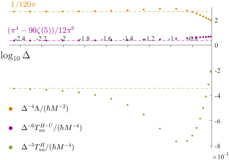
Figure 1: $\Lambda\Delta^{-4}$, $\left\langle T_{uu}^{-}\right\rangle_{\text{ren}}^{H}\Delta^{-5}$ and $\left\langle T_{uu}^{-}\right\rangle_{\text{ren}}^{H-U}\Delta^{-6}$ in suitable units vs. $\log_{10}\Delta$. The horizontal colored dashed lines correspond to the coefficients of the leading orders in $\Delta$, known analytically for $\Lambda$ and $\left\langle T_{uu}^{-}\right\rangle_{\text{ren}}^{H-U}$ as prescribed in Eqs. (III.2) and (III.3).

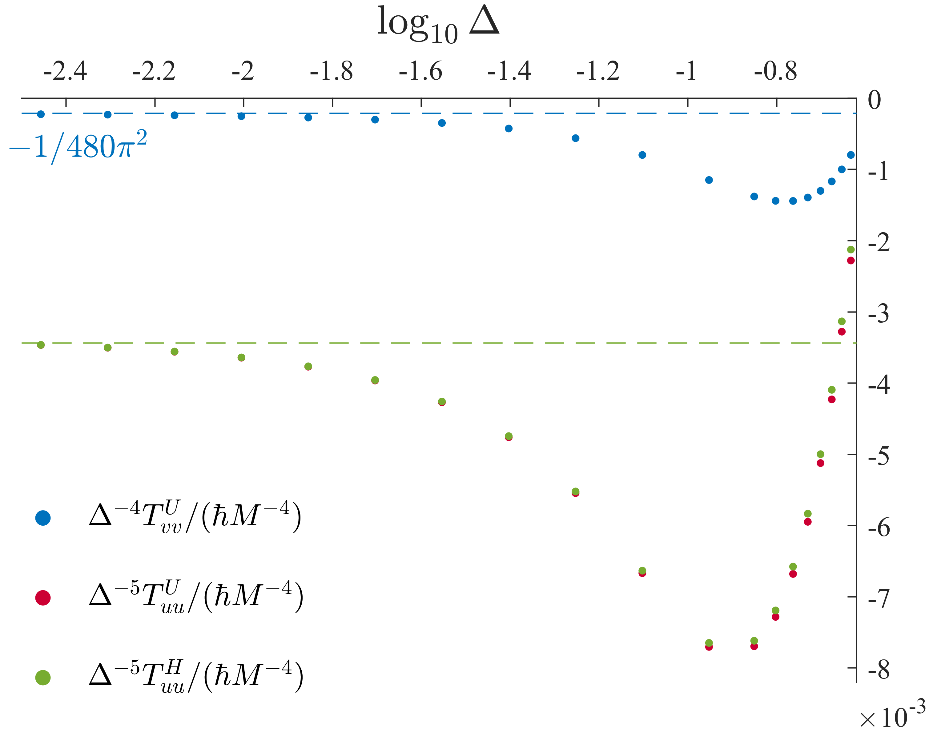
Figure 2: $\left\langle T_{vv}^{-}\right\rangle_{\text{ren}}^{U}\Delta^{-4}$, $\left\langle T_{uu}^{-}\right\rangle_{\text{ren}}^{H}\Delta^{-5}$ and $\left\langle T_{uu}^{-}\right\rangle_{\text{ren}}^{U}\Delta^{-5}$ in suitable units vs. $\log_{10}\Delta$. The horizontal colored dashed lines correspond to the coefficients of the leading orders in $\Delta$, known to be identical for $\left\langle T_{uu}^{-}\right\rangle_{\text{ren}}^{H}$ and $\left\langle T_{uu}^{-}\right\rangle_{\text{ren}}^{U}$ (see Eq. III.5), and known analytically for $\left\langle T_{vv}^{-}\right\rangle_{\text{ren}}^{U}$ as prescribed in Eq. (III.6).

V Discussion.

Our main goal in this paper was to investigate and compute the semiclassical null fluxes $\left\langle T_{uu}\right\rangle_{\text{ren}}$ and $\left\langle T_{vv}\right\rangle_{\text{ren}}$ at the IH of a near-extremal RN BH, in the Unruh and HH quantum states. Since in the HH state we have $\left\langle T_{vv}\right\rangle_{\text{ren}}=\left\langle T_{uu}\right\rangle_{\text{ren}}$, there are three such independent flux quantities: $\left\langle T_{uu}^{-}\right\rangle_{\text{ren}}^{U}$, $\left\langle T_{vv}^{-}\right\rangle_{\text{ren}}^{U}$, and $\left\langle T_{uu}^{-}\right\rangle_{\text{ren}}^{H}$. (Recall, the “$-$” superscript denotes the asymptotic IH value, and the superscripts “$U$” and “$H$” respectively refer to the Unruh and HH quantum states.) We referred to these three flux quantities as the elementary triplet of fluxes. We found it useful, however, to introduce another (yet mathematically equivalent) triplet of flux-related quantities: $\left\langle T_{uu}^{-}\right\rangle_{\text{ren}}^{H}$, $\Lambda$, and $\left\langle T_{uu}^{-}\right\rangle_{\text{ren}}^{H-U}$, to which we referred as the derived triplet. Here “$H-U$“ denotes the flux difference between the HH and Unruh states, and $\Lambda\equiv 4\pi r_{-}^{2}\left(\left\langle T_{uu}^{-}\right\rangle_{\text{ren}}^{U}-\left\langle T_{vv}^{-}\right\rangle_{\text{ren}}^{U}\right)$. Although the elementary and derived triplets in principle encode the same information, we found it beneficial to focus our analysis on the latter triplet, as it allows a sharper investigation of the near-extremal limit. Firstly, two out of the three members of the derived triplet, $\Lambda$ and $\left\langle T_{uu}^{-}\right\rangle_{\text{ren}}^{H-U}$, are amenable to a full leading-order analytical treatment near extremality. Furthermore, we find that the flux difference $\left\langle T_{uu}^{-}\right\rangle_{\text{ren}}^{H-U}$ decreases faster than both $\left\langle T_{uu}^{-}\right\rangle_{\text{ren}}^{H}$ and $\left\langle T_{uu}^{-}\right\rangle_{\text{ren}}^{U}$ on approaching extremality. As an additional motivation, $\Lambda$ turns out to be directly associated with the conserved quantity presented in Eq. (I.3), which in fact coincides with the Hawking-evaporation outflux to infinity (a point to be further discussed below).

We hereby summarize our findings for the asymptotic behavior of the various flux quantities, to leading order in the small parameter $\Delta\equiv\sqrt{1-\left(Q/M\right)^{2}}$ (which expresses the deviation from extremality). Considering first the derived triplet, we obtained analytical expressions for two of its members: $\Lambda\propto\Delta^{4}$ and $\left\langle T_{uu}^{-}\right\rangle_{\text{ren}}^{H-U}\propto\Delta^{6}$ (see Eqs. (III.2) and (III.3) respectively). For the third member we got a numerical result: $\left\langle T_{uu}^{-}\right\rangle_{\text{ren}}^{H}\propto\Delta^{5}$ (see Eq. (III.4)). Our analytical results (including both the leading-order powers of $\Delta$ and the corresponding prefactors) agree with the behavior seen in the numerically computed quantities, as portrayed in Fig. 1.

From these results we could easily obtain the leading-order behavior of the elementary triplet, namely the flux quantities $\left\langle T_{yy}^{-}\right\rangle_{\text{ren}}^{\Xi}$ (see Subsec. III.4). We quote our final results:

$$\left\langle T_{vv}^{-}\right\rangle_{\text{ren}}^{H}=\left\langle T_{uu}^{-}\right\rangle_{\text{ren}}^{H}\cong\left\langle T_{uu}^{-}\right\rangle_{\text{ren}}^{U}\cong\alpha\Delta^{5}\,\,\,,\,\,\,\left\langle T_{vv}^{-}\right\rangle_{\text{ren}}^{U}\cong-\hbar\frac{\Delta^{4}}{480\pi^{2}M^{4}}$$

where $\alpha$ is a coefficient extracted from the numerics to be $\alpha\cong-3.4375\times 10^{-3}\,\hbar M^{-4}$ (as indicated from the level of the horizontal dashed green line in e.g. Fig. 1).

These results may be intuitively understood as follows. At a nearly extremal RN BH, since the interior domain shrinks as the two horizons “approach one another” (as indicated by the similarity of their $r_{+}$ and $r_{-}$ values, which only differ by $2M\Delta$), the fluxes at the IH vicinity don’t differ much from their corresponding EH values. That is, since for an evaporating BH (in the Unruh state) we have $\left\langle T_{vv}\right\rangle_{\text{ren}}^{U}<0$ and $\left\langle T_{uu}\right\rangle_{\text{ren}}^{U}=0$ at the EH, we expect to find at the IH a negative $\left\langle T_{vv}^{-}\right\rangle_{\text{ren}}^{U}$ (similar in magnitude to its corresponding EH value), as well as $\left\langle T_{uu}^{-}\right\rangle_{\text{ren}}^{U}$ vanishing more rapidly than $\left\langle T_{vv}^{-}\right\rangle_{\text{ren}}^{U}$, as extremality is approached. In particular, this means the quantity $\Lambda$ is expected to be dominated by $\left\langle T_{vv}^{-}\right\rangle_{\text{ren}}^{U}$, and indeed we find the following approximate relation to hold near extremality: $\Lambda\cong-4\pi r_{-}^{2}\left\langle T_{vv}^{-}\right\rangle_{\text{ren}}^{U}$ (see Subsec. III.4).

Although our main interest in this paper concerns semiclassical physics deep inside the BH, in passing, we also derived the leading-order small-$\omega$ expression for $\tau_{\omega l}^{\text{up}}$, namely the transmission coefficient outside the BH (see Appendix). This coefficient is a necessary ingredient in the analysis of the near-IH flux differences $\left\langle T_{uu}^{-}\right\rangle_{\text{ren}}^{H-U}$ and $\Lambda$.

As was already mentioned, the quantity $4\pi r^{2}\left(\left\langle T_{uu}\right\rangle_{\text{ren}}-\left\langle T_{vv}\right\rangle_{\text{ren}}\right)$ is independent of $r$ in both HH and Unruh states. In the latter, at the IH it reduces to $\Lambda$ (given in Eq. (III.2)) whereas in the limit $r\to\infty$ it coincides with the Hawking-evaporation outflux. Thus, on passing we have obtained the explicit expression for the evaporation rate of a near-extremal RN BH:

$$\lim_{r\to\infty}4\pi r^{2}\left\langle T_{uu}^{U}\right\rangle_{\text{ren}}\cong\hbar\,\frac{\Delta^{4}}{120\pi M^{2}}\,.$$ (V.1)

While the scaling of this quantity as $\propto\Delta^{4}$ has already been pointed out in e.g. Ref. (Jacobson, ), we are not aware of previous derivations of the prefactor. The analytical computation of this prefactor, carried out in Subsec. III.1, was made possible due to our analysis of the transmission coefficient $\tau_{\omega l}^{\text{up}}$ at low frequencies (presented in the Appendix).

Returning to semiclassical fluxes inside the BH, our results indicate that for a near-extremal RN BH in the Unruh state, $\left\langle T_{vv}\right\rangle_{\text{ren}}^{U}$ dominates over $\left\langle T_{uu}\right\rangle_{\text{ren}}^{U}$ in the IH vicinity. This could suggest that the semiclassically back-reacted geometry in this domain may be well approximated by the ingoing charged Vaidya solution (BonnorVaidya:1970, ). We hope to further explore this issue in future research.

Appendix A The transmission coefficient in low frequencies.

In this appendix we analyze the leading order of the transmission coefficient $\tau_{\omega l}$ at low frequencies (namely, corresponding to modes with $\omega M\ll 1$), in a RN BH. We shall provide the full analysis for a subextremal BH (that is, with $Q/M<1$), which is of direct relevance for this paper, and then quote the analogous result for an extremal RN BH (with $Q/M=1$).

We shall consider the “in” mode normalized to have amplitude $1$ at the EH, denoted by $\hat{\psi}_{\omega l}$, which is a solution to the radial equation (I.1) in the BH exterior with the following asymptotic behavior:

$$\hat{\psi}_{\omega l}(r_{*})\cong\begin{cases}e^{-i\omega r_{*}}&r_{*}\to-\infty\\ \mathcal{T}_{\omega l}e^{-i\omega r_{*}}+\mathcal{R}_{\omega l}e^{i\omega r_{*}}&r_{*}\to\infty\end{cases}\,.$$ (A.1)

$\mathcal{T}_{\omega l}$ and $\mathcal{R}_{\omega l}$ may then be used to construct the usual reflection and transmission coefficients $\tau_{\omega l}$ and $\rho_{\omega l}$ of the standard “in” and “up” Eddington-Finkelstein modes (see Ref. (Group:2018, )). In the “in” modes, $\tau_{\omega l}^{\text{in}}$ and $\rho_{\omega l}^{\text{in}}$ are trivially related to $\mathcal{T}_{\omega l}$ and $\mathcal{R}_{\omega l}$ via:

$$\tau_{\omega l}^{\text{in}} =\frac{1}{\mathcal{T}_{\omega l}}\,\;,\,\;\rho_{\omega l}^{\text{in}}=\frac{\mathcal{R}_{\omega l}}{\mathcal{T}_{\omega l}}\,.$$ (A.2)

The corresponding “up” mode coefficients, $\tau_{\omega l}^{\text{up}}$ and $\rho_{\omega l}^{\text{up}}$, may be related to their “in” counterparts through the conserved Wronskian, yielding:

$$\tau_{\omega l}^{\text{up}}=\tau_{\omega l}^{\text{in}}=\frac{1}{\mathcal{T}_{\omega l}}\,\;,\,\;\rho_{\omega l}^{\text{up}}=-\rho_{\omega l}^{\text{in}*}\frac{\tau_{\omega l}^{\text{in}}}{\tau_{\omega l}^{*\text{in}}}=-\frac{\mathcal{R}_{\omega l}^{*}}{\mathcal{T}_{\omega l}}\,.$$ (A.3)

We denote $\tau_{\omega l}\equiv\tau_{\omega l}^{\text{in}}=\tau_{\omega l}^{\text{up}}$, and we take here the $r_{*}$ convention used in Ref. (Group:2018, ):

$$r_{*} =r+\frac{1}{2\kappa_{+}}\log\left(\frac{r-r_{+}}{r_{+}-r_{-}}\right)-\frac{1}{2\kappa_{-}}\log\left(\frac{r-r_{-}}{r_{+}-r_{-}}\right)\,.$$ (A.4)

The variation of the effective potential $V_{l}$ given in Eq. (I.2) between the EH ($r_{*}\to-\infty$) and infinity ($r_{*}\to\infty$) suggests a natural division of the BH exterior into three overlapping regions, in which suitable approximations can be made: region I at the EH vicinity, where the effect of the potential is negligible and we may approximate the radial function by a free solution $\psi\cong e^{-i\omega r_{*}}$ (a more detailed characterization of this region will follow); region II where $\omega$ is negligible in the radial equation, that is, the domain characterized by $\omega^{2}\ll V_{l}$; and region III, the asymptotically flat region, where $r/M\gg 1$. Note that due to our assumption of small frequencies region II is very vast and, as we shall see, indeed overlaps with both its neighboring regions. This, in turn, allows the matching procedure which follows, relating the asymptotic regions $r_{*}\to-\infty$ and $r_{*}\to\infty$. We shall start at the EH vicinity and work our way outwards to infinity, where the reflection and transmission coefficients are to be extracted.

A.0.1 Region I

We start our analysis at the asymptotic domain where the effective potential is negligible, satisfying $V_{l}\ll\omega^{2}$. This yields a free solution to the radial equation (I.1), which according to Eq. (A.1) is

$$\psi_{\omega l}^{\text{free}}=e^{-i\omega r_{*}}\,.$$ (A.5)

However, the domain characterized by $V_{l}\ll\omega^{2}$ has no overlap with region II, where, as mentioned above, $V_{l}\gg\omega^{2}$. We thus wish to “enhance” the free solution $\psi_{\omega l}^{\text{free}}$, in order to slightly extend its domain of validity. To build the enhanced free solution, we consider the leading order near-EH form of the potential, $V_{l}\cong v_{l}M^{-2}\exp\left(2\kappa_{+}r_{*}\right)$, where $v_{l}$ is a certain dimensionless constant . Correspondingly, we use the Ansatz

$$\psi_{\omega l}\cong\psi_{\omega l}^{\text{free}}\left[1+cM^{2}V_{l}\right]\cong e^{-i\omega r_{*}}\left[1+cv_{l}\exp\left(2\kappa_{+}r_{*}\right)\right]\,,$$

where $c$ is a dimensionless constant that will be determined by the radial equation as follows: Applying the differential operator $\text{d}^{2}/\text{d}r_{*}^{2}+(\omega^{2}-V_{l})$ to this Ansatz for $\psi_{\omega l}$ yields

$$\left[\text{d}^{2}/\text{d}r_{*}^{2}+(\omega^{2}-V_{l})\right]\psi_{\omega l}=e^{-i\omega r_{*}}V_{l}\left[4M^{2}\kappa_{+}\left(\kappa_{+}-i\omega\right)c-1\right]+\mathcal{O}(V_{l}^{2})\,.$$

Equating the right hand side to zero (ignoring the $\mathcal{O}(V_{l}^{2})$ term) yields $c=\left[4M^{2}\kappa_{+}\left(\kappa_{+}-i\omega\right)\right]^{-1}$. Thus, we find the near-EH solution (to leading order in $V_{l}$) to be

$$\psi_{\omega l}=e^{-i\omega r_{*}}\left[1+\frac{1}{4\kappa_{+}\left(\kappa_{+}-i\omega\right)}V_{l}\right]\,.$$ (A.6)

For later convenience, we also write its derivative with respect to $r_{*}$ (hereafter denoted by a prime):

$$\psi^{\prime}_{\omega l}=-i\omega e^{-i\omega r_{*}}\left[1-\frac{2\kappa_{+}-i\omega}{4i\omega\kappa_{+}\left(\kappa_{+}-i\omega\right)}V_{l}\right]\,.$$ (A.7)

The domain of validity of this approximation (which ignores terms of higher orders in $V_{l}$) is basically characterized by $M^{2}V_{l}\ll 1$. However, for our goal of subsequently matching this solution to region II, it will be convenient to further restrict region I such that both $\psi_{\omega l}$ and $\psi^{\prime}_{\omega l}$ are still not significantly affected by the potential $V_{l}$. (We are concerned about the forms of $\psi_{\omega l}$ as well as $\psi^{\prime}_{\omega l}$, because the matching of regions I and II will involve the values of both $\psi_{\omega l}$ and $\psi^{\prime}_{\omega l}$ in the overlap domain). Recalling that $\kappa_{+}\sim 1/M\gg\omega$, one readily sees that the more stringent restriction emerges from the expression for $\psi^{\prime}_{\omega l}$: The term in squared brackets in Eq. (A.7) reads $\approx 1-V_{l}/(2i\omega\kappa_{+})$ for small $\omega$, hence the demand that $\psi^{\prime}_{\omega l}$ remains well approximated by its free counterpart $\psi^{\prime}{}_{\omega l}^{\text{free}}=-i\omega e^{-i\omega r_{*}}$ yields the requirement

$$V_{l}\left(r\right)\ll\omega/M\,,\qquad r\approx r_{+}\qquad\qquad\qquad\text{(region I)}$$ (A.8)

. The last inequality guarantees that both $\psi^{\prime}_{\omega l}$ and $\psi_{\omega l}$ do not differ much from their free values $\psi^{\prime}{}_{\omega l}^{\text{free}}$ and $\psi_{\omega l}^{\text{free}}$. We thus take this inequality to characterize region I, and we denote the approximate solution therein by $\hat{\psi}_{\omega l}^{I}$. From the very construction of region I, we may simply take $\hat{\psi}_{\omega l}^{I}$ to be the free solution given in Eq. (A.5) .

Having $V_{l}\propto r-r_{+}$ in that domain, we may rewrite the condition in Eq. (A.8) as

$$\frac{r-r_{+}}{M}\ll\omega M\,.\qquad\qquad\qquad\text{(region I)}$$ (A.9)

Note that since $\omega M\ll 1$, the last inequality also ensures that region I is indeed at the EH vicinity, where the assumed near-EH form of the potential is valid.

A.0.2 Region II

This region is characterized by

$$V_{l}\left(r\right)\gg\omega^{2}\,,\qquad\qquad\qquad\text{(region II)}$$ (A.10)

and we may thus neglect $\omega^{2}$ in the radial equation (I.1) as a leading order approximation. This yields the so-called static solution,

$$\hat{\psi}_{\omega l}^{II}=\frac{r}{M}\left[C_{1}P_{l}\left(\frac{r-M}{r_{+}-M}\right)+C_{2}Q_{l}\left(\frac{r-M}{r_{+}-M}\right)\right]\,,$$ (A.11)

where $P_{l}$ and $Q_{l}$ are respectively the Legendre polynomial and Legendre function of the second kind , and $C_{1},C_{2}$ are coefficients to be determined. We shall treat $\hat{\psi}_{\omega l}^{II}$ as the approximate solution throughout region II.

Owing to the basic assumption of low frequencies $\omega M\ll 1$, region II (characterized in Eq. (A.10)) and region I (characterized in Eq. (A.8)) overlap in a domain satisfying

$$\left(\omega M\right)^{2}\ll V_{l}M^{2}\ll\omega M\,,\qquad r\approx r_{+}\qquad\qquad\qquad\text{(regions I-II overlap)}$$ (A.12)

or, from the near-EH form of $V_{l}$,

$$\left(\omega M\right)^{2}\ll\frac{r-r_{+}}{M}\ll\omega M\,.\qquad\qquad\qquad\text{(regions I-II overlap)}$$ (A.13)

In order to match the solutions $\hat{\psi}_{\omega l}^{I}$ and $\hat{\psi}_{\omega l}^{II}$ in the overlap domain characterized above, we apply the right side of the inequality (A.13) in $\hat{\psi}_{\omega l}^{II}$ and the left side of this inequality in $\hat{\psi}_{\omega l}^{I}$. In fact, it turns out to be sufficient (and equivalent) to take $r-r_{+}\ll M$ in $\hat{\psi}_{\omega l}^{II}$ and $|\omega r_{*}|\ll 1$ in $\hat{\psi}_{\omega l}^{I}$ .

Taking the solution $\hat{\psi}_{\omega l}^{I}$ given in Eq. (A.5) in the asymptotic domain of region I where $|\omega r_{*}|\ll 1$ yields:

$$\hat{\psi}_{\omega l}^{I}\left(|\omega r_{*}|\ll 1\right) \cong 1-i\omega r_{*}\cong 1-i\omega\left[r_{+}+\frac{r_{+}^{2}}{r_{+}-r_{-}}\log\left(\frac{r-r_{+}}{r_{+}-r_{-}}\right)\right]$$ (A.14)

$$\frac{\text{d}}{\text{d}r}\hat{\psi}_{\omega l}^{I}\left(|\omega r_{*}|\ll 1\right) \cong-i\omega\frac{r_{+}^{2}}{\left(r-r_{+}\right)\left(r_{+}-r_{-}\right)}\,.$$

Carrying the solution $\hat{\psi}_{\omega l}^{II}$ as given in Eq. (A.11) to the asymptotic domain of region II where $r-r_{+}\ll M$, and using the leading-order asymptotic behavior of our basis functions $P_{l}\left(x\to 1^{+}\right)=1$ and $Q_{l}\left(x\to 1^{+}\right)\cong\frac{1}{2}\ln\left(\frac{2}{x-1}\right)$ , we get

$$\hat{\psi}_{\omega l}^{II}\left(r-r_{+}\ll M\right) \cong\frac{r_{+}}{M}\left[C_{1}+\frac{1}{2}C_{2}\log\left(\frac{r_{+}-r_{-}}{r-r_{+}}\right)\right]$$ (A.15)

$$\frac{\text{d}}{\text{d}r}\hat{\psi}_{\omega l}^{II}\left(r-r_{+}\ll M\right) \cong-\frac{1}{2M}\frac{r_{+}}{r-r_{+}}C_{2}$$

regardless of $l$. Then, matching to Eq. (A.14) requires setting the coefficients $C_{1},C_{2}$ to their leading order in $\omega$ (which suffices for the present analysis) as follows:

$$C_{1}=\frac{M}{r_{+}}{\color[rgb]{0,0,1}}\,\,,\,\,C_{2}=2i\omega M\frac{r_{+}}{r_{+}-r_{-}}\,.$$

Feeding this in Eq. (A.11), the approximate solution in region II is found to be:

$$\hat{\psi}_{\omega l}^{II}=\frac{r}{r_{+}}P_{l}\left(\frac{r-M}{r_{+}-M}\right)+\frac{2i\omega r_{+}r}{r_{+}-r_{-}}Q_{l}\left(\frac{r-M}{r_{+}-M}\right)\,.$$ (A.16)

Finally, we explore the domain of validity of the region-II approximation in the range $r\gg M$. The basic criterion that needs to be satisfied in this region is given in Eq. (A.10), namely $V_{l}\left(r\right)\gg\omega^{2}$. At $r\gg M$, the effective potential $V_{l}$ given in Eq. (I.2) decays like $\propto 1/r^{2}$ for $l>0$ and like $\propto M/r^{3}$ for $l=0$. This implies that the corresponding domain of validity is $r/M\ll\left(\omega M\right)^{-1}$ for $l>0$ and $r/M\ll\left(\omega M\right)^{-2/3}$ for $l=0$. In the analysis that follows it will be convenient to treat the $l=0$ and $l>0$ cases on a common footing. We therefore choose the domain in which we apply the region-II approximation, in the range $r\gg M$, to be the stringent of these two domains (that is, the one emerging from the $l=0$ case):

$$r/M\ll\left(\omega M\right)^{-2/3}\,.\qquad\qquad\qquad\text{(region II, large-$r$ side)}$$ (A.17)

A.0.3 Region III

In the asymptotically flat region characterized by

$$r/M\gg 1\qquad\qquad\qquad\text{(region III)}$$ (A.18)

(which implies $f\left(r\right)\cong 1$, $\text{d}f/\text{d}r\cong 0$), the approximate solution is well known and is given in terms of spherical Bessel functions:

$$\hat{\psi}_{\omega l}^{III} =\omega r_{*}\left[D_{1}j_{l}\left(\omega r_{*}\right)+D_{2}y_{l}\left(\omega r_{*}\right)\right]\,,$$ (A.19)

where $j_{l}$ and $y_{l}$ are respectively the spherical Bessel functions of the first and second kind, and $D_{1},D_{2}$ are coefficients to be determined from the matching procedure.

We wish to match $\hat{\psi}_{\omega l}^{III}$ with the solution $\hat{\psi}_{\omega l}^{II}$ of region II. The overlap domain of regions II and III is obtained by combining the conditions (A.17) and (A.18), namely:

$$1\ll\frac{r}{M}\ll\left(\omega M\right)^{-2/3}\,.\qquad\qquad\qquad\text{(regions II-III overlap)}$$ (A.20)

This overlap domain indeed exists, owing to our basic assumption $\omega M\ll 1$. Furthermore, a direct consequence of Eq. (A.20) is $r/M\ll\left(\omega M\right)^{-1}$ and therefore:

$$\omega r\ll 1\,.$$ (A.21)

We find it convenient to describe the matching in the overlap domain to be between $\hat{\psi}_{\omega l}^{III}$ in the asymptotic domain of region III where $\omega r_{*}\ll 1$, and $\hat{\psi}_{\omega l}^{II}$ in the asymptotic domain of region II where $r/M\gg 1$. The large-$r$ limit of $\hat{\psi}_{\omega l}^{II}$ (given in Eq. (A.16)) is obtained from the asymptotic behavior of $P_{l}\left(x\right)$ and $Q_{l}\left(x\right)$ at a large argument, namely $P_{l}\left(x\to\infty\right)\cong\left(2x\right)^{l}\frac{\Gamma\left(l+\frac{1}{2}\right)}{l!\sqrt{\pi}}$ and $Q_{l}\left(x\to\infty\right)\cong\left(2x\right)^{-l-1}\frac{l!\sqrt{\pi}}{\Gamma\left(l+\frac{3}{2}\right)}$. Inserting that into Eq. (A.16) yields:

$$\hat{\psi}_{\omega l}^{II}\left(r/M\gg 1\right)\cong r^{l+1}\frac{1}{r_{+}}\left(\frac{2}{r_{+}-M}\right)^{l}\frac{\Gamma\left(l+\frac{1}{2}\right)}{\sqrt{\pi}l!}+r^{-l}\frac{2i\omega r_{+}}{r_{+}-r_{-}}\frac{\sqrt{\pi}l!}{\Gamma\left(l+\frac{3}{2}\right)}\left(\frac{2}{r_{+}-M}\right)^{-l-1}\,.$$ (A.22)

Plugging the asymptotic behavior of the spherical Bessel functions of the first and second kinds at a small argument in Eq. (A.19), we obtain:

$$\hat{\psi}_{\omega l}^{III}\left(\omega r_{*}\ll 1\right)\cong\omega r_{*}\left[D_{1}\left(\omega r_{*}\right)^{l}\frac{\sqrt{\pi}}{\Gamma\left(\frac{3}{2}+l\right)}2^{-l-1}-D_{2}\left(\omega r_{*}\right)^{-l-1}\frac{1}{\sqrt{\pi}}2^{l}\Gamma\left(l+\frac{1}{2}\right)\right]\,,$$ (A.23)

Note that the dependence on $r$ in the last two equations is only through simple powers of $r$ or $r_{*}$. We can then re-express these two equations in the more compact form

$$\hat{\psi}_{\omega l}^{III}\left(\omega r_{*}\ll 1\right)\cong\tilde{D}_{1}r_{*}^{l+1}+\tilde{D}_{2}r_{*}^{-l}$$

$$\hat{\psi}_{\omega l}^{II}\left(r/M\gg 1\right)\cong\tilde{C}_{1}r^{l+1}+\tilde{C}_{2}r^{-l}$$

(where the new coefficients $\tilde{C}_{i},\tilde{D}_{i}$ are trivially related to $C_{i},D_{i}$ by comparing the above to Eqs. (A.22,A.23)). Obviously, the large-$r$ assumption allows replacing $r_{*}^{l+1}$ with $r^{l+1}$ and $r_{*}^{-l}$ with $r^{-l}$, as the relative error decays like $\propto\frac{M}{r}\log\left(\frac{r}{M}\right)\ll 1$. The matching then simply yields $\tilde{D}_{1}=\tilde{C}_{1}$ and $\tilde{D}_{2}=\tilde{C}_{2}$. Applying this straightforward matching scheme to Eqs. (A.22,A.23) determines the desired coefficients $D_{1},D_{2}$ (to their leading order in $\omega$):

$$D_{1}=\lambda_{l}\left(\omega M\right)^{-l-1}\,\,,\,\,D_{2}=-i\lambda_{l}^{-1}\left(\omega M\right)^{l+1}$$ (A.24)

where

$$\lambda_{l}=\frac{M}{r_{+}}\left(\frac{8M}{r_{+}-r_{-}}\right)^{l}\frac{2\Gamma\left(l+\frac{1}{2}\right)\Gamma\left(l+\frac{3}{2}\right)}{\pi l!}\,.$$ (A.25)

Feeding Eq. (A.24) into Eq. (A.19), we obtain the approximate solution throughout region III:

$$\hat{\psi}_{\omega l}^{III} =\omega r_{*}\left[\lambda_{l}\left(\omega M\right)^{-l-1}j_{l}\left(\omega r_{*}\right)-i\lambda_{l}^{-1}\left(\omega M\right)^{l+1}y_{l}\left(\omega r_{*}\right)\right]\,.$$ (A.26)

A.0.4 Asymptotic behavior at $r\to\infty$

Finally, in order to extract $\mathcal{T}_{\omega l}$ and $\mathcal{R}_{\omega l}$, we need to match $\hat{\psi}_{\omega l}^{III}$ to the boundary condition (A.1) at $r_{*}\to\infty$. That is, we are interested in the asymptotic behavior of $\hat{\psi}_{\omega l}^{III}$ where $\omega r_{*}\gg 1$. Using $j_{l}\left(x\to\infty\right)\cong-\frac{1}{x}\sin\left(\frac{l\pi}{2}-x\right)$ and $y_{l}\left(x\to\infty\right)\cong-\frac{1}{x}\cos\left(\frac{l\pi}{2}-x\right)$ in Eq. (A.19), we obtain:

$$\hat{\psi}_{\omega l}^{III}\left(\omega r_{*}\gg 1\right)\cong-D_{1}\sin\left(\frac{l\pi}{2}-\omega r_{*}\right)-D_{2}\cos\left(\frac{l\pi}{2}-\omega r_{*}\right)\,.$$ (A.27)

At the $\omega M\ll 1$ limit, the coefficient $D_{2}\propto\left(\omega M\right)^{l+1}$ is negligible compared to $D_{1}\propto\left(\omega M\right)^{-l-1}$ (see Eq. (A.24)), and we are left with:

$$\hat{\psi}_{\omega l}^{III}\left(\omega r_{*}\gg 1\right) \cong-\lambda_{l}\left(\omega M\right)^{-l-1}\sin\left(\frac{l\pi}{2}-\omega r_{*}\right)$$

$$=\frac{\lambda_{l}}{2}\left(\omega M\right)^{-l-1}i^{l+1}\left[e^{-i\omega r_{*}}+\left(-1\right)^{l+1}e^{i\omega r_{*}}\right]\,.$$ (A.28)

With the above asymptotic form, we can easily read the coefficients $\mathcal{T}_{\omega l}$ and $\mathcal{R}_{\omega l}$ as appearing in Eq. (A.1):

$$\mathcal{T}_{\omega l}=\frac{\lambda_{l}}{2}\left(\omega M\right)^{-l-1}i^{l+1}\,\,\,\,,\,\,\,\,\mathcal{R}_{\omega l}=\frac{\lambda_{l}}{2}\left(\omega M\right)^{-l-1}\left(-1\right)^{l+1}i^{l+1}\,.$$

Then, via the relations in Eqs. (A.2,A.3), one can readily extract the reflection and transmission coefficients to leading order in low frequencies:

$$\rho_{\omega l}^{\text{in}}\cong\left(-1\right)^{l+1}\,\,,\,\,\rho_{\omega l}^{\text{up}}\cong-1$$ (A.29)

and

$$\tau_{\omega l}\cong\frac{\pi r_{+}}{M}\left(\frac{r_{+}-r_{-}}{8M}\right)^{l}\frac{l!}{\Gamma\left(l+\frac{1}{2}\right)\Gamma\left(l+\frac{3}{2}\right)}\left(-i\right)^{l+1}\left(\omega M\right)^{l+1}\,,$$ (A.30)

or, using $\Gamma\left(\frac{1}{2}+l\right)=\frac{\left(2l\right)!}{4^{l}l!}\sqrt{\pi}$:

$$\tau_{\omega l}\cong\frac{r_{+}}{M}\left(\frac{r_{+}-r_{-}}{M}\right)^{l}\frac{2^{l+2}\left(l!\right)^{2}\left(l+1\right)!}{\left(2l\right)!\left(2l+2\right)!}\left(-i\right)^{l+1}\left(\omega M\right)^{l+1}\,.$$ (A.31)

One immediate consequence is that the leading order of $\tau_{\omega l}$ in small frequencies is real when $l$ is odd and imaginary when $l$ is even. In particular, for the sake of this paper, note that for $l=0$ we have to leading order

$$\tau_{\omega,l=0}\cong-2i\omega r_{+}\,.$$ (A.32)

The results presented here were verified numerically – both for $l=0$ as given in Eq. (A.32) and for several other $l$ values as given more generally in Eq. (A.31) – in a variety of subextremal $Q/M$ values.

In the Schwarzschild limit ($r_{-}\to 0$, $r_{+}\to 2M$), Eq. (A.31) adequately reduces to the corresponding result given in Eq. (5.5) of Ref. (CasalsOttewill:2015, ).

Note that the results presented in Eqs. (A.29,A.31) were derived in the subextremal RN case only, and they are not valid for an extremal BH. We shall briefly refer to the extremal case in the subsection that follows.

The transmission coefficient in low frequencies in an extremal RN BH

An analysis analogous to the one presented in detail above can be done in the extremal case. Since the two horizons now coincide at $r=M$, this changes the behavior of $f\left(r\right)$, and hence also $r_{*}$, $V_{l}\left(r\right)$, and the corresponding solutions in the various domains. Nevertheless, despite these differences, the basic strategy presented above is applicable in the extremal case as well: We can again define the three domains with three corresponding approximate solutions (the enhanced free solution in the EH vicinity, the static solution where $V_{l}\gg\omega^{2}$, and the large-$r$ solution), with appropriate overlapping domains in which any two of the neighboring approximate solutions may be matched. Then, matching through and taking the $r_{*}\to\infty$ limit, we finally obtain the asymptotic behavior (analogous to Eq. (A.28) in the subextremal case):

$$\hat{\psi}_{\omega l}^{III}\left(\omega r_{*}\gg 1\right)\cong-\frac{i}{M}\left(\frac{2}{M}\right)^{2l}\Gamma\left(l+\frac{1}{2}\right)\Gamma\left(l+\frac{3}{2}\right)\frac{1}{\pi}\omega^{-2l-1}\left[\left(-1\right)^{l+1}e^{-i\omega r_{*}}+e^{i\omega r_{*}}\right]\,.$$ (A.33)

We may now use Eqs. (A.2,A.3) to extract the transmission and reflection coefficients to leading order in small frequencies for an extremal RN BH:

$$\rho_{\omega l}^{\text{in}}\cong\rho_{\omega l}^{\text{up}}\cong\left(-1\right)^{l+1}$$ (A.34)

$$\tau_{\omega l}\cong i\left(-1\right)^{l+1}\frac{\pi}{2^{2l}}\frac{1}{\Gamma\left(l+\frac{1}{2}\right)\Gamma\left(l+\frac{3}{2}\right)}\left(\omega M\right)^{2l+1}\,.$$ (A.35)

Note that the leading order of $\tau_{\omega l}$ in low frequencies is $\propto\left(\omega M\right)^{2l+1}$ in the extremal case (unlike $\left(\omega M\right)^{l+1}$ in the subextremal case, see Eq. (A.31)), and that it is always imaginary.

- (1) N. Zilberman, A. Levi and A. Ori, Quantum Fluxes at the Inner Horizon of a Spherical Charged Black Hole, Phys. Rev. Lett. 124, 171302 (2020).
- (2) J. B. Hartle and S. W. Hawking, Path-integral derivation of black-hole radiance, Phys. Rev. D. 13, 2188 (1976).
- (3) W. Israel, Thermo-field dynamics of black holes, Phys. Lett. A. 57, 107 (1976).
- (4) W. G. Unruh, Notes on black-hole evaporation, Phys. Rev. D. 14, 870 (1976).
- (5) S. Hollands, R. M. Wald and J. Zahn, Quantum instability of the Cauchy horizon in Reissner-Nordström-deSitter spacetime, Phys. Rev. D. 98, 024025 (2018).
- (6) T. Jacobson, Semiclassical Decay of Near-Extremal Black Holes, Phys. Rev. D. 57, 4890 (1998).
- (7) A Levi and A. Ori, Mode-sum regularization of in the angular-splitting method, Phys. Rev. D. 94, 044054 (2016).
- (8) A. Levi, Stress-energy tensor mode-sum regularization in spherically symmetric backgrounds, in preparation.
- (9) A. Levi and A. Ori, Pragmatic mode-sum regularization method for semiclassical black-hole spacetimes, Phys. Rev. D. 91, 104028 (2015).
- (10) A. Levi and A. Ori, Versatile Method for Renormalized Stress-Energy Computation in Black-Hole Spacetimes, Phys. Rev. Lett. 117, 231101 (2016).
- (11) A. Levi, Renormalized stress-energy tensor for stationary black holes, Phys. Rev. D. 95, 025007 (2017).
- (12) A. Lanir, A. Levi, A. Ori and O. Sela, Two-point function of a quantum scalar field in the interior region of a Reissner-Nordstrom black hole, Phys. Rev. D. 97, 024033 (2018).
- (13) B. S. DeWitt, Quantum field theory in curved spacetime, Phys. Rep. C. 19, 295 (1975).
- (14) S. M. Christensen and S. A. Fulling, Trace anomalies and the Hawking effect, Phys. Rev. D. 15, 2088 (1977).
- (15) W. B. Bonnor and P. C. Vaidya, Spherically symmetric radiation of charge in Einstein-Maxwell theory, Gen. Rel. Grav. 1(2), pp. 127-130 (1970).
- (16) M. Casals and A. C. Ottewill, High-order tail in Schwarzschild spacetime, Phys. Rev. D. 92, 124055 (2015).