Training Neural Networks with an algorithm for piecewise linear functions
Abstract.
We present experiments on training neural networks with an algorithm that was originally designed as a subgradient method, namely the Volume Algorithm. We compare with two of the most frequently used algorithms like Momentum and Adam. We also compare with the newly proposed algorithm COCOB.
Key words and phrases:
Training neural networks; Subgradient method; Volume algorithm.1. Introduction
The Volume Algorithm [2] is a subgradient method designed for minimizing a convex piecewise linear function, later it was extended to convex non-differentiable functions in [1]. Since its publication in 2000 it has showed better convergence than the traditional subgradient method [9], and it has been particularly useful for large-scale instances for which other algorithms have been impractical, see [8], [7], for instance. For these reasons we decided to adapt it for deep learning where high-order optimization methods are not suitable, and to compare it with gradient descent methods. Here we should mention that for instance, the popular ReLu activation function is piece-wise linear and non-differentiable, so a subgradient method is well suited for this case. We should also mention that in most neural networks the loss function is not convex, then any method designed for minimizing convex functions becomes a heuristic, and its performance has to be evaluated in an experimental fashion. Here we present experiments with several different types of neural networks. In the final section we present a summary of the results in Table 1, which shows that the Volume Algorithm is robust and compares very well with the others. To make our results easy to reproduce we restrict our experiments to several publicly available neural networks, also we make our code available as open-source in a GitHub repository [3].
Stochastic gradient descent [18], [11], and its relatives like AdaGrad [6], RMSProp [26], Adam [12], Momentum [17] are among the most frequently used algorithms in machine learning; see [19] for more references. Also recently COCOB has been proposed in [15] with promising results. Here we compare the Volume algorithm with two of the most commonly used methods, namely Momentum and Adam. We also include COCOB in this comparison. We chose Adam according to the survey [19] that in Section 4.10 reads ‘Kingma et al. [12] show that its bias-correction helps Adam slightly outperform RMSprop towards the end of optimization as gradients become sparser. Insofar, Adam might be the best overall choice’. We chose Momentum because it is widely used. We also included COCOB because it is a new algorithm that does not require an initial learning rate, and it has been reported in [15] that COCOB has a training performance that is on-par or better than state-of-the-art algorithms.
The remainder of this paper is as follows. In Section 2 we describe the Volume Algorithm. Section 3 contains our experiments. In Section 4 we give some final remarks.
2. The Volume Algorithm
We start with an example to motivate the choice of the direction in our method, and then we describe the algorithm.
2.1. An example
Suppose that we want to maximize the piecewise linear function below
Consider the point . Here we have . Thus at the point the function has the subgradients and . Notice that the direction that gives the largest improvement per unit of movement is . It can be obtained as a convex combination of the subgradients above as . Now we discuss how to obtain the coefficients of this convex combination. Notice that the area of the triangle with vertices , , is , and the area of the triangle with vertices , , is . Thus if we use each of these areas divided by the sum of the areas we obtain the coefficients of the convex combination, see Figure 1. In higher dimensions we should use volumes instead of areas. In the next subsection we shall see that this procedure is not particular to this example, but it corresponds to a method to obtain the direction of improvement using volumes.

2.2. Volume and duality
Now we give a theoretical justification for what we did in the example above. Recall that maximizing a concave piecewise linear function can be written as
| (1) | |||
| subject to | |||
| (2) |
The following theorem was published in [2].
Theorem 1.
Consider the linear program (1)-(2), let be an optimal solution, and suppose that constraints , , are active at this point. Let and assume that
defines a bounded polyhedron. For , let be the volume between the face defined by and the hyperplane defined by . The shaded region in Figure 2 illustrates such a volume. Then an optimal dual solution is given by

Roughly speaking, this theorem suggests that given a vector one should look at the active faces, and compute the volume of their projection over the hyperplane , on a neighborhood of , and for some small value of . Let be the face defined by , and let be the ratio of the volume below the face to the total. Then one should compute
If this is the vector of all zeroes, we have a proof of optimality, otherwise we have a direction of improvement, see Figure 3. This is similar to what we did in the previous example. In the next subsection we present an algorithm that computes approximations of these volumes.

2.3. The Algorithm
As previously suggested, for a vector , we could try a set of random points in the hyperplane defined by . For each of these points we can identify the face above it. Theorem 1 suggests that we should look at the coefficients as the probabilities that the different faces will appear. Thus we look at the coefficients as the probabilities that a subgradient method will produce the different subgradients . Then to compute the direction of improvement we propose the keep a direction and update it in every iteration as
| (3) |
where is the last subgradient produced, and is a small value. Therefore if is the sequence of subgradients produced, the direction is
The coefficients of this convex combination are an approximation of the values of Theorem 1. This update scheme is similar to the one used in Adam [12], the difference with our algorithm is in the choice of the step-size. As we shall see in the next section, this makes a significant difference in terms of convergence.
Once the direction has been chosen, ideally we would do a line search, but since this is prohibitively expensive, we use the following scheme. Suppose we use a step size , and let be the new subgradient obtained. If the inner product is positive, this means that the step size was too small, a larger step size would have resulted on a better solution. We call this a “green” iteration. If is negative, this means that a smaller step size would have given a better solution. We call this a “yellow” iteration. Then we keep a “green-yellow” indicator that is a number between and . At each green iteration we update as . At each yellow iteration we update as . Each time that we increase the step size. When we decrease the step size. We see this as low cost approximation of a line search.
Now we can describe the algorithm, it was published first in [2], and a proof of convergence was given in [1].
Volume Algorithm
-
•
Input: We assume that we have to maximize a function of variables . We also receive a value , and an initial step-size . We set upper an upper bound for the step-size , and and a lower bound . Initially we set .
At each iteration we keep a vector that corresponds to a direction. We initialize it to be equal to the first subgradient. At each iteration we receive a new subgradient that is used to update the direction. The different steps are below.
-
•
Step 1. Compute . This is the inner product of the direction and the new subgradient.
If increase as
otherwise decrease as
If increase as .
If decrease as .
If , set . If , set .
Update the direction as -
•
Step 2. Update the variables as
Go to Step 1.
This is for maximization, if we want to minimize we update the variables as In our experiments we used .
3. Experiments
Here we compare the Volume Algorithm with three of the most frequently used methods, namely Momentum [17], Adam [12] and RMSProp [26], we also compare with the new algorithm COCOB [15]. For the first three algorithms we used their implementation found in [21], for COCOB we used the implementation in [4]. The Volume Algorithm was implemented in TensorFlow. For the choice of the learning rate, for each algorithm we looked for the best value in . This set of values was used in [15] for their comparisons. Recall that COCOB has the interesting feature of not requiring an initial learning rate. In the figures below we show the best learning rate used for each algorithm. For Adam we used and . For Momentum we used for the momentum value.
We used seven test sets available in the public domain, as follows. We have downloaded tensorflow implementations of different neural networks in the public domain. We used the same number of steps, epochs, batch-size, etc., as in these implementations. We make our code publicly available in [3], and thus these experiments are easy to reproduce.
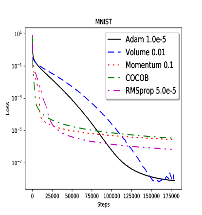
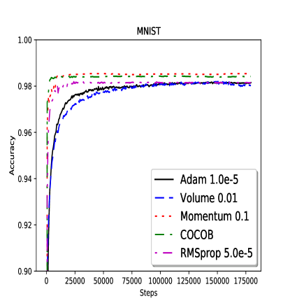
3.1. MNIST
This is a well known digits-recognition dataset, see [14]. We used the neural network implemented in [4]. In Figure 4 we plot train loss and accuracy as functions of the number of steps.
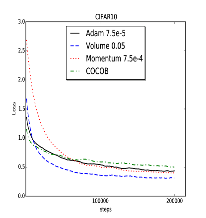
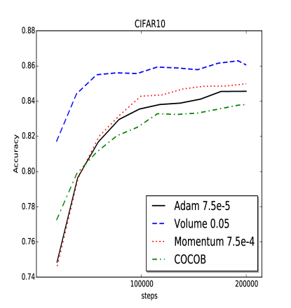
3.2. CIFAR10
This is a dataset for classifying 32x32 RGB images across 10 object categories, see [5]. Here we used the code from the TensorFlow tutorial [23]. In Figure 5 we plot train loss and accuracy as functions of the number of steps.
3.3. Recurrent Neural Networks
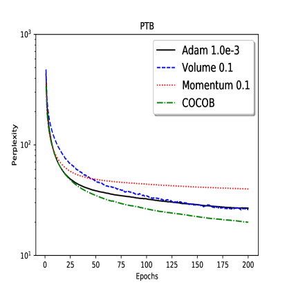
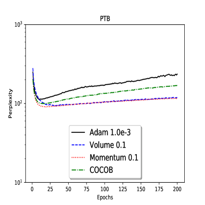
Here we use the Penn Tree Bank dataset [16] to train a Recurrent Neural Network. The goal is to predict next words in a text given a history of previous words. We use the code in the TensorFlow tutorial [25]. In Figure 6 we plot perplexity as a function of epochs for the train set and for the test set.
3.4. Retraining Inception V3
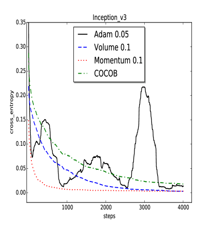
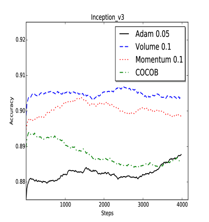
Here we use a model trained on the Imagenet dataset [10] to classify images of flowers. We use the code from TensorFlow for Poets [24] to download a pre-trained model, add a new final layer, and train that layer on a set of flower photos. Here we use an Inception V3 model, see [20]. In Figure 7 we plot cross entropy for the training set, and accuracy for the evaluation set as a function of the number of steps.
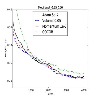
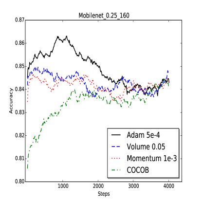
3.5. Retraining Mobilenet_0.25_160
This time we retrain using a Mobilenet model [13]. The relative size of the model is 0.25 and the image size is 160. In Figure 8 we plot cross entropy for the training set, and accuracy for the evaluation set as a function of the number of steps.
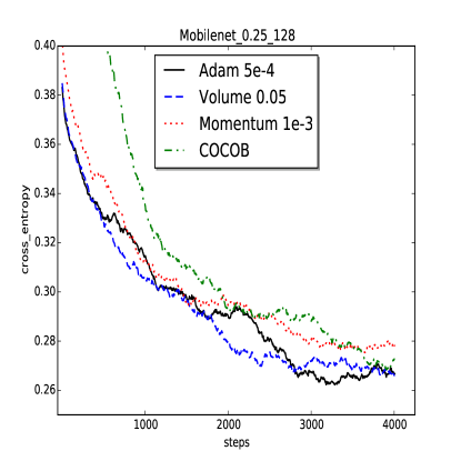
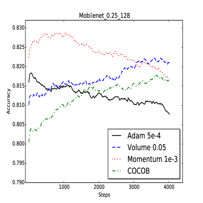
3.6. Retraining Mobilenet_0.25_128
Here we retrained using a Mobilenet model [13]. The relative size of the model is 0.25 and the image size is 128. In Figure 9 we plot cross entropy for the training set, and accuracy for the evaluation set as a function of the number of steps.
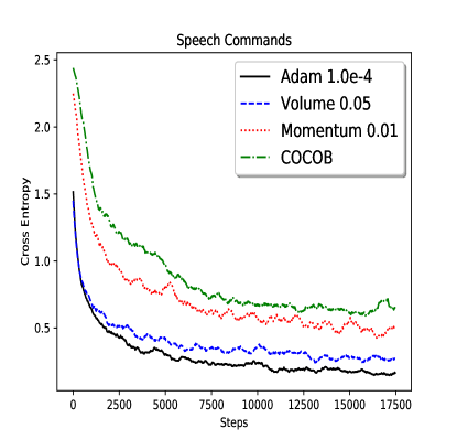
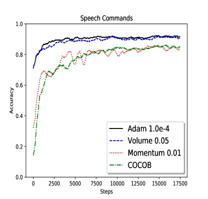
3.7. Simple Audio Recognition
Here we use a basic speech recognition network that recognizes ten different words from the TensorFlow tutorial [22]. In Figure 10 we plot cross entropy for the training set, and accuracy for the evaluation set as a function of the number of steps.
4. Final Remarks
We have presented a comparison of several algorithms for training neural networks. In Table 1 we give labels from 1 to 4 to display the order from best to worst of the different algorithms on each dataset. If for one dataset several algorithms have been best, we give the label 1 to each of them. The Volume Algorithm received the label 1 five times and the label 2 two times.
| MNIST | CIFAR10 | PTB | Inc V3 | Mb_.25_160 | Mb_.25_128 | Audio | |
|---|---|---|---|---|---|---|---|
| Adam | 2 | 3 | 2 | 3 | 1 | 1 | 1 |
| Momentum | 3 | 2 | 4 | 1 | 1 | 4 | 3 |
| COCOB | 4 | 4 | 1 | 4 | 4 | 1 | 4 |
| Volume | 1 | 1 | 2 | 1 | 1 | 1 | 2 |
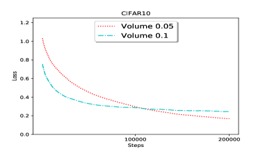
The choice of the direction in our algorithm is similar to the one for Adam, however the choice of the step-size makes a significant difference, see Figure 7 for instance. In our case we input an initial value and allow the step-size to vary in the interval . In Figure 11 we show the behavior of the Volume Algorithm for two different values of , namely the values and . For the larger value the function decreases faster in the earlier steps, and tends to stabilize later. For the smaller value the decrease is slower in the early steps, but it does not stabilize until later. This suggests a strategy of using one interval for the early steps, and later switch to an interval containing smaller values for the later steps. The design of such strategy will be the subject of future research.
acknowledgments
We are grateful Mark Wegman for his helpful comments on the preparation of this paper.
References
- [1] L. Bahiense, N. Maculan, and C. Sagastizábal, The volume algorithm revisited: relation with bundle methods, Mathematical Programming, 94 (2002), pp. 41–69.
- [2] F. Barahona and R. Anbil, The volume algorithm: producing primal solutions with a subgradient method, Mathematical Programming, 87 (2000), pp. 385–399.
- [3] F. Barahona and J. Goncalves, Volume optimizer for tensorflow. https://github.com/IBM/volume-optimizer-for-tensorflow.
- [4] CCB, COCOB. https://github.com/bremen79/cocob.
- [5] CIFAR-10, The CIFAR-10 dataset. https://www.cs.toronto.edu/~kriz/cifar.html.
- [6] J. Duchi, E. Hazan, and Y. Singer, Adaptive subgradient methods for online learning and stochastic optimization, Journal of Machine Learning Research, 12 (2011), pp. 2121–2159.
- [7] L. F. Escudero, M. Landete, and A. M. Rodriguez-Chia, Stochastic set packing problem, European Journal of Operational Research, 211 (2011), pp. 232–240.
- [8] O. Günlük, T. Kimbrel, L. Ladanyi, B. Schieber, and G. B. Sorkin, Vehicle routing and staffing for sedan service, Transportation Science, 40 (2006), pp. 313–326.
- [9] M. Held, P. Wolfe, and H. P. Crowder, Validation of subgradient optimization, Mathematical programming, 6 (1974), pp. 62–88.
- [10] IN, IMAGENET. http://image-net.org/.
- [11] J. Kiefer and J. Wolfowitz, Stochastic estimation of the maximum of a regression function, The Annals of Mathematical Statistics, (1952), pp. 462–466.
- [12] D. P. Kingma and J. Ba, Adam: A method for stochastic optimization, arXiv preprint arXiv:1412.6980, (2014).
- [13] MN, MobileNets: Open-Source Models for Efficient On-Device Vision. https://ai.googleblog.com/2017/06/mobilenets-open-source-models-for.html.
- [14] MNIST, The MNIST database of handwritten digits. http://yann.lecun.com/exdb/mnist/.
- [15] F. Orabona and T. Tommasi, Training deep networks without learning rates through coin betting, in Advances in Neural Information Processing Systems, 2017, pp. 2157–2167.
- [16] PTB, Treebank-3. https://catalog.ldc.upenn.edu/ldc99t42.
- [17] N. Qian, On the momentum term in gradient descent learning algorithms, Neural networks, 12 (1999), pp. 145–151.
- [18] H. Robbins and S. Monro, A stochastic approximation method, The annals of mathematical statistics, (1951), pp. 400–407.
- [19] S. Ruder, An overview of gradient descent optimization algorithms, arXiv preprint arXiv:1609.04747, (2016).
- [20] C. Szegedy, V. Vanhoucke, S. Ioffe, J. Shlens, and Z. Wojna, Rethinking the inception architecture for computer vision, CoRR, abs/1512.00567 (2015).
- [21] TF, TensorFlow. https://www.tensorflow.org/.
- [22] TFaudio, Simple Audio Recognition. https://www.tensorflow.org/versions/master/tutorials/audio_recognition.
- [23] TFcifar10, Convolutional Neural Networks. https://www.tensorflow.org/tutorials/deep_cnn.
- [24] TFpoets, TensorFlow For Poets. https://codelabs.developers.google.com/codelabs/tensorflow-for-poets/#0.
- [25] TFptb, Recurrent Neural Networks. https://www.tensorflow.org/versions/master/tutorials/recurrent.
- [26] T. Tieleman and G. Hinton, Lecture 6.5-rmsprop, coursera: Neural networks for machine learning, University of Toronto, Technical Report, (2012).