Global constraints on neutral-current generalized neutrino interactions

Abstract

We study generalized neutrino interactions (GNI) for several neutrino processes, including neutrinos from electron-positron collisions, neutrino-electron scattering, and neutrino deep inelastic scattering. We constrain scalar, pseudoscalar, and tensor new physics effective couplings, based on the standard model effective field theory at low energies. We have performed a global analysis for the different effective couplings. We also present the different individual constraints for each effective parameter (scalar, pseudoscalar, and tensor). Being a global analysis, we show robust results for the restrictions on the different GNI parameters and improve some of these bounds.

I Introduction

Precision neutrino physics experiments have successfully determined the standard three-neutrino oscillation picture parameters. Future long-baseline neutrino experiments such as DUNE Abi et al. (2020) and Hyper-K Abe et al. (2015) will measure this phase accurately. Current neutrino data allows an exhaustive search on physics beyond the Standard Model (SM) of Particle Physics. The attempts to explain the neutrino mass pattern implies models with new interactions that modify the Standard Model Lagrangian and predict different values for its vector and axial couplings, a deviation that can be described by the neutrino non-standard interactions (NSI) formalismOhlsson (2013); Miranda and Nunokawa (2015); Farzan and Tortola (2018); Dev (2019). Besides, electromagnetic neutrino properties could give a clear signature of new physics if a non-zero neutrino magnetic moment exists Giunti and Studenikin (2015); Miranda et al. (2019). This tensor interaction could be tested in the future, for example, in dark matter direct detection experiments Aristizabal Sierra et al. (2020). Other kinds of physics beyond the Standard Model, such as leptoquark models Buchmuller et al. (1987); Crivellin et al. (2020); Gargalionis and Volkas (2021), also contain modifications to the usual couplings and predict new scalar couplings. Moreover, motivated by experimental data, special attention has been given to scalar neutrino interactions through solar neutrino measurements from Borexino Ge and Parke (2019); Khan et al. (2020), and even from astrophysical and cosmological observations like BBN, CMB, and supernovae Heurtier and Zhang (2017); Huang et al. (2018); Forastieri et al. (2019); Escudero and Witte (2020); Venzor et al. (2021).

From a phenomenological perspective, we can study all these different interactions in a model-independent framework by considering all the couplings allowed by the effective field theory. Such a picture is known as generalized neutrino interactions (GNI) and it can be considered as an extension of the non-standard interaction framework. In the GNI case, we consider the appearance of scalar, pseudoscalar, and tensor couplings, besides the possible modification to the vector and axial couplings (also considered in NSI).

Generalized Neutrino Interactions have been recently studied using measurements from decay branching ratios, $\beta$ decay, and neutrino scattering off electrons and quarks Bischer and Rodejohann (2019a, b); Han et al. (2020); Li et al. (2020a); Chen et al. (2021), as well as from coherent elastic neutrino-nucleus scattering Lindner et al. (2017); Papoulias and Kosmas (2018); Aristizabal Sierra et al. (2018); Li et al. (2020b). In this work, we perform a global analysis of different neutrino processes in order to constrain neutral-current GNI parameters. Besides these global constraints, we will also report several new individual constrains. In particular, we use data from neutrino-electron scattering, neutrino Deep Inelastic Scattering (DIS), and single-photon detection from electron-positron collisions.

This work is organized as follows. In Sec. II, we present the general formalism of the generalized neutrino interactions and the relevant cross-sections for our analysis. In Sec. III, we provide a brief description of various neutrino experiments used in this work, their relevant observables, and the $\chi^{2}$ adopted for each of them. We report our constraints for each experimental observable in Sec. IV. We also show, in the same section, the global limits on the GNI parameters. Finally we summarize and give our conclusions in Sec. V.

II The generalized interactions formalism and cross-sections

We introduce in this section the GNI framework that we will use in our study. The natural approach is to consider an effective field theory that includes new physics and that, at the electroweak scale, respects the $SU(3)_{\mathrm{C}}\times SU(2)_{\mathrm{L}}\times U(1)_{\mathrm{Y}}$ gauge group. This approach is usually known as the standard model effective field theory (SMEFT) Buchmuller and Wyler (1986); Grzadkowski et al. (2010). We will adopt this scheme in our analysis.

We will consider that, additional to the Standard Model Lagrangian, we can have contributions from the most general effective Lagrangian for neutral currents that is given by the following four-fermion interaction Bischer and Rodejohann (2019b); Han et al. (2020); Bischer and Rodejohann (2019a),

$$\mathcal{L}^{NC}_{eff}=-\frac{G_{F}}{\sqrt{2}}\sum_{j}\epsilon^{f,j}_{\alpha\beta}(\bar{\nu}_{\alpha}\mathcal{O}_{j}\nu_{\beta})(\bar{f}\mathcal{O}^{{}^{\prime}}_{j}f)\,,\\$$ (1)

where $G_{F}$ is the Fermi coupling constant, $f$ represents a fermion with a given flavor, and $\nu_{\alpha\beta}$ a (anti)neutrino with flavor $\alpha,\beta$. The operators $\mathcal{O}_{j}$ and $\mathcal{O}^{{}^{\prime}}_{j}$ account for the generalized interactions that are explicitly shown in Table 1. These operators are assumed to have an effective strength given by the couplings $\epsilon^{f,j}_{\alpha\beta}$ for left-handed neutrino interactions. An even more general picture would include the embedding of right-handed neutrinos del Aguila et al. (2009); Aparici et al. (2009). For the case of Dirac neutrinos, the right-handed components would be mandatory and may lead to additional constraints if new interactions are considered, such as in the case of the effective number of neutrino species in the early Universe Luo et al. (2020) or they may even help to disentangle the Dirac vs Majorana nature Rodejohann et al. (2017). However, this is out of the scope of this work. Several analyses have set constraints on some of this additional coefficients using different measurements from LHC, LEP, and the projected sensitivities from future collider facilities Ruiz (2017); Cai et al. (2018); Alcaide et al. (2019); Biekötter et al. (2020).

In defining the Lagrangian in Eq. (1) we have adopted a convention that is commonly used for these couplings. For a different convention we refer the reader to the Appendix A. It could be possible to return back to a Lagrangian where the couplings are more transparent for the reader. For example, we can see that in the case of a pseudoscalar coupling we have

$$\bar{\nu}_{\alpha}(1-\gamma^{5})\nu_{\beta}\bar{f}\gamma^{5}f=2\bar{\nu}_{\alpha R}\nu_{\beta L}\bar{f}\gamma^{5}f,$$ (2)

where the pseudoscalar nature of this term is evident in the right-hand side of the previous equation. Analogous relations can be found for the rest of the couplings, where the differences restrict to proportionality constants. An exception is the case of the left and right-handed couplings ($L,R$) that are linear combinations of the $V,A$ couplings and coincide with those in the non-standard interactions (NSI) formalism.

The Lagrangian in Eq. (1) is added to the Standard Model Lagrangian, that have the left and right handed couplings

$$g^{L,SM} = 1+\left(-\frac{1}{2}+s^{2}_{W}\right),$$

$$g^{R,SM} = s^{2}_{W},$$ (3)

where $s_{W}$ is the sine of the weak mixing angle.

${\epsilon}$		$\mathcal{O}_{j}$		$\mathcal{O}^{{}^{\prime}}_{j}$
$\epsilon^{f,L}$		$\gamma_{\mu}(1-\gamma^{5})$		$\gamma^{\mu}(1-\gamma^{5})$
$\epsilon^{f,R}$		$\gamma_{\mu}(1-\gamma^{5})$		$\gamma^{\mu}(1+\gamma^{5)}$
$\epsilon^{f,S}$		$(1-\gamma^{5})$		$1$
$-\epsilon^{f,P}$		$(1-\gamma^{5})$		$\gamma^{5}$
$\epsilon^{f,T}$		$\sigma_{\mu\nu}(1-\gamma^{5})$		$\sigma^{\mu\nu}(1-\gamma^{5})$

Table 1: Effective operators and effective couplings in Eq. (1) studied in this work.

In this work we will compute constraints for the scalar, pseudoscalar, and tensor interactions. We will focus in left(right) handed (anti)neutrinos. In the case of vector and axial couplings (or left and right handed chiralities) there are already several works in the literature where a current status can be found Ohlsson (2013); Miranda and Nunokawa (2015); Farzan and Tortola (2018). For the sake of completeness, we remind here some of the most relevant constraints for these couplings.

The most stringent constraint reported in the literature restrict the muon neutrino couplings, as muon neutrino fluxes are abundant in accelerator experiments . For flavor diagonal couplings, the constraints for beyond the Standard Model interactions with electrons are Davidson et al. (2003); Barranco et al. (2008)

$$|\epsilon^{e,L}_{\mu\mu}|<3\times 10^{-2},\quad|\epsilon^{e,R}_{\mu\mu}|<3\times 10^{-2},$$ (4)

and

$$|\epsilon^{e,L}_{\mu\tau}|<0.13,\quad|\epsilon^{e,R}_{\mu\tau}|<0.13.$$ (5)

For the interactions with quarks, the constraints are given, at $90$ % CL by Escrihuela et al. (2011)

$$|\epsilon^{d,V}_{\mu\mu}|<0.042,\quad|\epsilon^{d,A}_{\mu\mu}|<0.057,$$ (6)

while for the flavor changing case we have

$$|\epsilon^{q,V}_{\mu\tau}|<7\times 10^{-3},\quad|\epsilon^{q,A}_{\mu\tau}|<39\times 10^{-3}.$$ (7)

In the case of interactions with electrons, the most stringent constraint on the right-handed coupling comes from the TEXONO reactor antineutrino experiment, while for the left-handed coupling a combination of solar and KamLAND experiments provides the stronger limit Barranco et al. (2008); Bolanos et al. (2009); Deniz et al. (2010a):

$$-0.021<\epsilon^{e,L}_{ee}<0.052,\quad-0.07<\epsilon^{e,R}_{ee}<0.08,$$ (8)

and

$$|\epsilon^{e,L}_{e\tau}|<0.33,\quad|\epsilon^{e,R}_{e\tau}|<0.19.$$ (9)

For the interactions with quarks, the constraints for electron neutrinos are given by Davidson et al. (2003)

$$|\epsilon^{d,L}_{ee}|<0.3,\quad-0.6<\epsilon^{d,R}_{ee}<0.5,$$ (10)

while for the flavor changing case we have the constraints Davidson et al. (2003)

$$|\epsilon^{q,L}_{e\tau}|<0.5,\quad|\epsilon^{q,R}_{e\tau}|<0.5.$$ (11)

Finally, the tau neutrino case have less stringent constraints. For the interaction with electrons they are given by Barranco et al. (2008); Bolanos et al. (2009)

$$-0.12<\epsilon^{e,L}_{\tau\tau}<0.06,\quad-0.25<\epsilon^{e,R}_{\tau\tau}<0.43,$$ (12)

and Davidson et al. (2003)

$$|\epsilon^{e,L}_{\mu\tau}|<0.1,\quad|\epsilon^{e,R}_{\mu\tau}|<0.1.$$ (13)

For the interaction with quarks, the flavor-diagonal constraint is Gonzalez-Garcia et al. (2011)

$$|\epsilon^{q,V}_{\tau\tau}|<0.037,$$ (14)

while for the flavor-changing case Escrihuela et al. (2011)

$$|\epsilon^{q,L}_{\mu\tau}|<23\times 10^{-3},\quad|\epsilon^{q,R}_{\mu\tau}|<36\times 10^{-3}.$$ (15)

Once we have overviewed the current status for the NSI parameters, we can turn our attention to the scalar, pseudoscalar, and tensor GNI parameters. We start by defining the relevant cross-sections for our study and their modification when a GNI parameter is present.

II.1 Cross-section for $e^{+}e^{-}\rightarrow\nu\bar{\nu}\gamma$

The neutrino-antineutrino pair produced together with a single photon is a clean signal measured with precision at LEP Barate et al. (1998a, b); Heister et al. (2003); Abreu et al. (2000); Acciarri et al. (1997, 1998, 1999); Ackerstaff et al. (1998); Abbiendi et al. (1999, 2000). This experimental result has been previously studied to put constraints on NSI Berezhiani and Rossi (2002); Barranco et al. (2008); Forero and Guzzo (2011) and non-unitarity Escrihuela et al. (2020), for instance.

To compute the GNI contributions for this observable, we must consider that its cross-section is written as the product Nicrosini and Trentadue (1989); Barranco et al. (2008); Berezhiani and Rossi (2002)

$$\frac{d^{2}\sigma}{dx\,dy}=H(x,y;s)\,\sigma_{0}(s(1-x)),$$ (16)

where $H(x,y;s)$ is the radiator function

$$H(x,y;s)=\frac{2\alpha\left[(1-\frac{1}{2}x)^{2}+\frac{1}{4}x^{2}y^{2}\right]}{\pi x(1-y^{2})},$$ (17)

with

$$x=2E_{\gamma}/\sqrt{s},\quad\quad y=\cos\theta_{\gamma},$$ (18)

where $\sqrt{s}$ is the center-of-mass energy and $E_{\gamma}(\theta_{\gamma})$ is the energy (angle) of the produced photon. The term $\sigma_{0}$ is the “reduced” cross-section for $e^{+}e^{-}\to\nu\bar{\nu}$,

$$\sigma_{0}(s) =\sigma_{W}(s)+\sigma_{Z}(s)+\sigma_{W-Z}(s),$$

$$\sigma_{0}(s) =\frac{{G_{F}}^{2}s}{12\pi}\left[2+\frac{N_{\nu}(g_{V}^{2}+g_{A}^{2})}{(1-s/{M_{Z}}^{2})^{2}+\Gamma_{Z}^{2}/M_{Z}^{2}}+\frac{2(g_{V}+g_{A})(1-s/{M_{Z}}^{2})}{(1-s/M_{Z}^{2})^{2}+\Gamma_{Z}^{2}/M_{Z}^{2}}\right],$$ (19)

where $\Gamma_{Z}$ and $M_{Z}$ are the $Z$ boson decay width and mass, respectively, and $N_{\nu}$ is the number of neutrino species. The first term in the previous equation comes from the $W$ contribution to the cross-section while the second one from the $Z$ contribution, as is illustrated in the Feynman diagrams in Fig. (1). The third contribution appears from the interference between both gauge bosons.

(a)

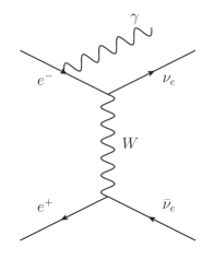
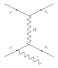
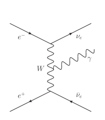
(b)

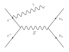
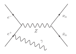
Figure 1: Contributions to the $e^{-}e^{+}\to\nu\bar{\nu}\gamma$ process at tree level, from the $W$ (a) and $Z$ (b) bosons.

Considering only neutral current GNI, we notice that the corrections to this interaction will come from diagrams that in the SM are related to the $Z$ bosons (Fig. 1). From Eq. (1) we can obtain the GNI cross-section contribution for the process

$$\sigma_{0}=\frac{G^{2}_{F}s}{48\pi}\sum_{\alpha,\beta}\left(8|\epsilon^{e,L}_{\alpha\beta}|^{2}+8|\epsilon^{e,R}_{\alpha\beta}|^{2}+3|\epsilon^{e,S}_{\alpha\beta}|^{2}+3|\epsilon^{e,P}_{\alpha\beta}|^{2}+32|\epsilon^{e,T}_{\alpha\beta}|^{2}\right)\,.$$ (20)

In Eq. (20), we can see that tensor interactions contribute one order of magnitude more to the cross-section than the equally-contributing scalar and pseudoscalar interactions.

With this information we can proceed to compute the total cross-section

$$\sigma(s)=\int_{x_{\mathrm{min}}}^{1}dx\int_{-\cos\theta_{\mathrm{min}}}^{\cos\theta_{\mathrm{min}}}dyH(x,y;s)\,\sigma_{0}(s(1-x)).$$ (21)

In the case of energies above the $Z$ resonance, it is important to consider finite distance effects on the $W$ propagator. They require the substitution Hirsch et al. (2003); Barranco et al. (2008); Berezhiani and Rossi (2002):

$$\sigma_{W}(s)\; \to\;\;\sigma_{W}(s)F_{W}(s/M_{W}^{2}),$$

$$\sigma_{W-Z}(s)\; \to\;\;\sigma_{W-Z}(s)F_{W-Z}(s/M_{W}^{2}),$$ (22)

with

$$F_{W}(z) =\frac{3}{z^{3}}\left[-2(z+1)\log(z+1)+z(z+2)\right],$$

$$F_{W-Z}(z) =\frac{3}{z^{3}}\left[(z+1)^{2}\log(z+1)-z(3z/2+1)\right].$$ (23)

From Eq. (20), we can notice that the GNI observable that can be studied from this process is the following

$$|\epsilon_{all}^{e,Y}|^{2}\equiv\sum_{\alpha,\beta}|\epsilon_{\alpha\beta}^{e,Y}|^{2},$$ (24)

where $Y=S,P,T$. Given that a neutrino-antineutrino pair is produced, this signal provides access to all the electron flavor-diagonal and flavor-changing GNI parameters.

II.2 Differential cross-section for the process $\nu_{\alpha}+e^{-}\rightarrow\nu_{\beta}+e^{-}$

The scattering of muon neutrinos off electrons is a purely leptonic process that has been measured Hasert et al. (1973) since the formulation of the SM. The small cross-section in comparison with the scattering off nuclei makes it challenging to have high-statistics samples. However, the clean leptonic signal yields independent information complementary to that of the quark sector.

For electron neutrinos, it is difficult to have clean neutrino fluxes at accelerator or spallation neutron sources. Therefore, the measurement of this cross-section has been done mainly with reactor antineutrino sources Reines et al. (1976); Daraktchieva et al. (2005); Vidyakin et al. (1992); Derbin et al. (1993) that have even lower statistics.

From Eq. (1), we obtain the following result for the differential cross-section for the process $\nu_{\alpha}+e^{-}\rightarrow\nu_{\beta}+e^{-}$, Bischer and Rodejohann (2019a)

$$\frac{d\sigma}{dE_{r}}=\frac{G^{2}_{F}m_{e}}{\pi}\left[A+2B\left(1-\frac{E_{r}}{E_{\nu}}\right)+C\left(1-\frac{E_{r}}{E_{\nu}}\right)^{2}+D\frac{m_{e}E_{r}}{E_{\nu}^{2}}\right]\,,$$ (25)

where $E_{r}$ is the kinetic energy of the recoiling electron and

$$A = 2|\epsilon^{e,L}_{\alpha\beta}|^{2}+\frac{1}{4}(|\epsilon^{e,S}_{\alpha\beta}|^{2}+|\epsilon^{e,P}_{\alpha\beta}|^{2})+8|\epsilon^{e,T}_{\alpha\beta}|^{2}-2\Re((\epsilon^{e,S}+\epsilon^{e,P})_{\alpha\beta}\epsilon^{e,T*}_{\alpha\beta})\,,$$

$$B = -\frac{1}{4}(|\epsilon^{e,S}_{\alpha\beta}|^{2}+|\epsilon^{e,P}_{\alpha\beta}|^{2})+8|\epsilon^{e,T}_{\alpha\beta}|^{2}\,,$$

$$C = 2|\epsilon^{e,R}_{\alpha\beta}|^{2}+\frac{1}{4}(|\epsilon^{e,S}_{\alpha\beta}|^{2}+|\epsilon^{e,P}_{\alpha\beta}|^{2})+8|\epsilon^{e,T}_{\alpha\beta}|^{2}+2\Re((\epsilon^{e,S}+\epsilon^{e,P})_{\alpha\beta}\epsilon^{e,T*}_{\alpha\beta})\,,$$

$$D = -2\Re(\epsilon^{e,L}_{\alpha\beta}\epsilon^{e,R*}_{\alpha\beta})+\frac{1}{2}|\epsilon^{e,S}_{\alpha\beta}|^{2}-8|\epsilon^{e,T}_{\alpha\beta}|^{2}\,.$$ (26)

For the case of antineutrinos, the interchange $A\leftrightarrow C$ has to be made in Eq. (25). From the definitions in Eq. (II.2), we notice that scalar and pseudoscalar interactions contribute equally to the cross-section, except for the last term, D, where there is only scalar contribution. Given that this contribution is inversely proportional to $E_{\nu}^{2}$ (last term of Eq. (25)), we could distinguish between scalar and pseudoscalar parameters in low-energy neutrino experiments.

Since the final (anti)neutrino flavor is unknown in an actual experiment, one has to sum over all the possible flavor outcomes. For this reason, the accessible observable for this process is

$$|\epsilon_{\alpha}^{e,Y}|^{2}\equiv\sum_{\beta}|\epsilon_{\alpha\beta}^{e,Y}|^{2}.$$ (27)

II.3 Neutrino-quark scattering

Besides neutrino-electron scattering, neutrino-quark scattering gives higher statistics measurements Dorenbosch et al. (1986); Allaby et al. (1987); Blondel et al. (1990); Zeller et al. (2002), although one must take the uncertainties due to sea-quark corrections with care.

We will analyze the cross-section for the process $\nu q\rightarrow\nu q$. The following expressions give the neutrino-nucleon scattering cross-sections for the charged and neutral weak currents in the SM Zyla et al. (2020)

$$\sigma^{CC}_{\nu N,SM}=\frac{G^{2}_{F}s}{2\pi}\left[f_{q}+\frac{1}{3}f_{\bar{q}}\right]\,,$$ (28)

$$\begin{split}\sigma^{\nu N}_{NC,SM}=&\frac{G^{2}_{F}s}{2\pi}\Big{[}\left((g^{u,L})^{2}+\frac{1}{3}(g^{u,R})^{2}\right)f_{q}+\left((g^{d,L})^{2}+\frac{1}{3}(g^{d,R})^{2}\right)f_{q}\\ &+\left((g^{u,R})^{2}+\frac{1}{3}(g^{u,L})^{2}\right)f_{\bar{q}}+\left((g^{d,R})^{2}+\frac{1}{3}(g^{d,L})^{2}\right)f_{\bar{q}}\Big{]}\,,\end{split}$$ (29)

and for the antineutrino-nucleon scattering, we have the analog formulas

$$\sigma^{CC}_{\bar{\nu}N,SM}=\frac{G^{2}_{F}s}{2\pi}\left[\frac{1}{3}f_{q}+f_{\bar{q}}\right]\,,$$ (30)

$$\begin{split}\sigma^{\bar{\nu}N}_{NC,SM}=&\frac{G^{2}_{F}s}{2\pi}\Big{[}\left((g^{u,R})^{2}+\frac{1}{3}(g^{u,L})^{2}\right)f_{q}+\left((g^{d,R})^{2}+\frac{1}{3}(g^{d,L})^{2}\right)f_{q}\\ &+\left((g^{u,L})^{2}+\frac{1}{3}(g^{u,R})^{2}\right)f_{\bar{q}}+\left((g^{d,L})^{2}+\frac{1}{3}(g^{d,R})^{2}\right)f_{\bar{q}}\Big{]}\,,\end{split}$$ (31)

where the SM effective couplings $g^{f,L}$ and $g^{f,R}$ are:

$$g^{f,L}=T^{f}_{3}-Q_{f}\sin^{2}\theta_{W}\,,\,\,\,\,\,\,g^{f,R}=-Q_{f}\sin^{2}\theta_{W}.$$ (32)

Following Ref. Erler and Su (2013), we have,

$$g^{u,L}=0.3457\,,\,\,\,\,g^{u,R}=-0.1553\,,\,\,\,\,g^{d,L}=-0.4288\,,\,\,\,\,g^{d,R}=0.0777\,.$$ (33)

Furthermore, assuming an isoscalar target, $f_{q}$ and $f_{\bar{q}}$ are nuclear PDFs that regulate the fraction of proton momentum carried by the up and down quarks and anti-quarks, respectively. Neglecting the contributions of heavy quarks, we have $f_{q}\equiv f_{d}+f_{u}=\int_{0}^{1}x[u(x)+d(x)]dx$, and $f_{\bar{q}}=f_{\bar{d}}+f_{\bar{u}}=\int_{0}^{1}x[\bar{u}(x)+\bar{d}(x)]dx$.
The modifications introduced by the presence of scalar, pseudoscalar, and tensor interactions are given by Han et al. (2020)

$$\sigma^{NC}_{\nu N,S(P)}=\sigma^{NC}_{\bar{\nu}N,S(P)}=\frac{G^{2}_{F}s}{24\pi}\left[\left(\epsilon^{u,S(P)}_{\alpha}\right)^{2}\left(\frac{f_{q}+f_{\bar{q}}}{2}\right)+\left(\epsilon^{d,S(P)}_{\alpha}\right)^{2}\left(\frac{f_{q}+f_{\bar{q}}}{2}\right)\right]\,,$$ (34)

$$\sigma^{NC}_{\nu N,T}=\sigma^{NC}_{\bar{\nu}N,T}=\frac{28G^{2}_{F}s}{3\pi}\left[\left(\epsilon^{u,T}_{\alpha}\right)^{2}\left(\frac{f_{q}+f_{\bar{q}}}{2}\right)+\left(\epsilon^{d,T}_{\alpha}\right)^{2}\left(\frac{f_{q}+f_{\bar{q}}}{2}\right)\right]\,,$$ (35)

where we have defined the effective couplings with quarks

$$|\epsilon_{\alpha}^{q,Y}|^{2}\equiv\sum_{\beta}|\epsilon_{\alpha\beta}^{q,X}|^{2}.$$ (36)

III Experimental observables

There is a large diversity of neutrino experiments that can provide constraints to GNI couplings. In the present work we focus on the “neutrino counting” experiments ALEPH Barate et al. (1998a, b); Heister et al. (2003), DELPHI Abreu et al. (2000), L3 Acciarri et al. (1997, 1998, 1999), and OPAL Ackerstaff et al. (1998); Abbiendi et al. (1999, 2000), the accelerator experiments CHARM Dorenbosch et al. (1986); Allaby et al. (1987), CHARM-II Vilain et al. (1993, 1994), CDHS Blondel et al. (1990), and NuTeV Zeller et al. (2002), and the reactor experiment TEXONO Deniz et al. (2010b). These experiments can probe different GNI couplings depending on the involved neutrino flavor and which fermion interacts with them. In the following, we will separate the experiments mentioned above according to the underlying process while describing the implemented analysis and the fitted observable.

III.1 Electron-positron collision

A neutrino-antineutrino pair, along a single photon, can be produced in electron-positron collisions, as can be seen in the diagrams of Fig. 1. Therefore, single-photon measurements can be used to derive limits to additional neutrino interactions. The LEP experiments ALEPH, DELPHI, L3, and OPAL had reported single-photon measurements at different energies above the $W^{-}W^{+}$ production threshold. In Table 2 we present the required data to perform the analysis. In order of appearance, each column consists of the center-of-mass energy, measured cross-section, expected cross-section reported by each collaboration, number of events after background subtraction, and the kinematic cuts on energy and angle of the produced photon. For the last two columns, $x_{T}=x\sin\theta_{\gamma}$, $x=E_{\gamma}/E_{\mathrm{beam}}$, and $y=\cos\theta_{\gamma}$.

		$\sqrt{s}$ (GeV)	$\sigma^{\mathrm{meas}}$ (pb)	$\sigma^{\mathrm{MC}}$ (pb)	$N_{\mathrm{obs}}$	$E_{\gamma}$ (GeV)	$|y|$
ALEPH	Barate et al. (1998a)	161	$5.3\pm 0.83$	$5.81\pm 0.03$	41	$x_{T}\geq 0.075$	$\leq 0.95$
		172	$4.7\pm 0.83$	$4.85\pm 0.04$	36	$x_{T}\geq 0.075$	$\leq 0.95$
	Barate et al. (1998b)	183	$4.32\pm 0.34$	$4.15\pm 0.03$	195	$x_{T}\geq 0.075$	$\leq 0.95$
	Heister et al. (2003)	189	$3.43\pm 0.17$	$3.48\pm 0.05$	484	$x_{T}\geq 0.075$	$\leq 0.95$
		192	$3.47\pm 0.40$	$3.23\pm 0.05$	81
		196	$3.03\pm 0.23$	$3.26\pm 0.05$	197
		200	$3.23\pm 0.22$	$3.12\pm 0.05$	231
		202	$2.99\pm 0.29$	$3.07\pm 0.05$	110
		205	$2.84\pm 0.22$	$2.93\pm 0.05$	182
		207	$2.67\pm 0.17$	$2.80\pm 0.05$	292
DELPHI	Abreu et al. (2000)	189	$1.80\pm 0.20$	$1.97$	146	$x\geq 0.06$	$\leq 0.7$
		183	$2.33\pm 0.36$	$2.08$	65	$x\geq 0.02$	$\leq 0.85$
		189	$1.89\pm 0.22$	$1.94$	155	$x\leq 0.9$	$\leq 0.98$
L3	Acciarri et al. (1997)	161	$6.75\pm 0.93$	$6.26\pm 0.12$	57	$\geq 10$	$\leq 0.73$
						and	and
		172	$6.12\pm 0.90$	$5.61\pm 0.10$	49	$E_{T}\geq 6$	0.80-0.97
	Acciarri et al. (1998)	183	$5.36\pm 0.40$	$5.62\pm 0.10$	195	$\geq 5$	$\leq 0.73$
						and	and
	Acciarri et al. (1999)	189	$5.25\pm 0.23$	$5.29\pm 0.06$	572	$E_{T}\geq 5$	0.80-0.97
OPAL	Ackerstaff et al. (1998)	130	$10.0\pm 2.34$	$13.48\pm 0.22$	19	$x_{T}>0.05$	$\leq 0.82$
						and	and
		136	$16.3\pm 2.89$	$11.30\pm 0.20$	34	$x_{T}>0.1$	$\leq 0.966$
	Abbiendi et al. (1999)	130	$11.6\pm 2.53$	$14.26\pm 0.06$	21	$x_{T}>0.05$	$\leq 0.966$
		136	$14.9\pm 2.45$	$11.95\pm 0.07$	39
	Ackerstaff et al. (1998)	161	$5.30\pm 0.83$	$6.49\pm 0.08$	40	$x_{T}>0.05$	$\leq 0.82$
						and	and
		172	$5.50\pm 0.83$	$5.53\pm 0.08$	45	$x_{T}>0.1$	$\leq 0.966$
	Abbiendi et al. (1999)	183	$4.71\pm 0.38$	$4.98\pm 0.02$	191	$x_{T}>0.05$	$\leq 0.966$
	Abbiendi et al. (2000)	189	$4.35\pm 0.19$	$4.66\pm 0.03$	643	$x_{T}>0.05$	$\leq 0.966$

Table 2: Data summary from the ALEPH, DELPHI, L3, and OPAL experiments.

The constraints on different GNI couplings can be obtained by performing a $\chi^{2}$ analysis with the function

$$\chi^{2}_{e^{-}e^{+}}=\sum_{i}\left(\frac{\sigma_{i}^{\mathrm{th}}-\sigma_{i}^{\mathrm{meas}}}{\sigma_{i}}\right)^{2}.$$ (37)

Here, $\sigma_{i}^{\mathrm{th}}$ is the theoretical cross-section including new interactions, which can be computed by integrating Eq. (21) in the limits shown in the last two columns of Table 2. The measured cross-section $\sigma_{i}^{\mathrm{meas}}$ and its uncertainty $\sigma_{i}$ can be read from the second column of Table 2. The subscript $i$ stands for the different measurements of each experiment. Given the details of the experimental cuts, we include a normalization factor with a $10\%$ systematic uncertainty in order to improve the robustness of the analysis Escrihuela et al. (2020).

III.2 Neutrino-electron scattering

The CHARM-II experiment has measured the neutrino-electron scattering cross-section from a purely neutral-current interaction Vilain et al. (1993, 1994). A total of $2677\pm 82$ $\nu_{\mu}e^{-}$ and $2752\pm 88$ $\bar{\nu}_{\mu}e^{-}$ events were detected using $\nu_{\mu}$ and $\bar{\nu}_{\mu}$ beams produced at CERN, with mean energies of 23.7 and 19.1 GeV, respectively.

To perform a fit over the GNI parameters, we use only the spectral information on the cross section reported by the experiment. We define the following function

$$\chi^{2}_{\mathrm{CHARM-II}}=\sum_{i=1}^{8}\left(\frac{(\tfrac{d\sigma}{dT})_{i}^{\mathrm{th}}-(\tfrac{d\sigma}{dT})_{i}^{\mathrm{meas}}}{\sigma_{i}}\right)^{2},$$ (38)

where $(\tfrac{d\sigma}{dT})_{i}^{\mathrm{th}}$ is the theoretical cross-section (including GNI) from Eq. (25), $(\tfrac{d\sigma}{dT})_{i}^{\mathrm{meas}}$ is the experimental measurement, and $\sigma_{i}$ its uncertainty Vilain et al. (1993). The subscript $i$ runs over all the neutrino (one to four) and antineutrino (five to eight) measurements.

The TEXONO collaboration has measured the $\bar{\nu}_{e}e^{-}$ scattering cross section using a CsI(Tl) scintillating crystal detector placed near the reactor at the Kuo-Sheng Nuclear Power Plant Deniz et al. (2010b). Events in the $3-8$ MeV recoil energy range were reported, resulting in 414 $\pm$ 80(stat) $\pm$ 61(syst) events in ten electron recoil energy bins, after background subtraction.

In order to extract limits for GNI, we use again only the event rate spectral information. We adopt the following least-squares function

$$\chi^{2}_{\mathrm{TEXONO}}=\sum_{i=1}^{10}\left(\frac{N_{i}^{\mathrm{th}}-N_{i}^{\mathrm{meas}}}{\sigma_{i}}\right)^{2},$$ (39)

where $N_{i}^{\mathrm{th}}$ is the theoretical number of events, while $N_{i}^{\mathrm{meas}}$ refers to the measured number of events in the $i$-th recoil energy bin, and $\sigma_{i}$ is the measured uncertainty Deniz et al. (2010b). The theoretical number of events is computed according to

$$N_{i}^{\mathrm{th}}=A\int_{E_{r}^{i}}^{E_{r}^{i+1}}\int_{E_{\nu}^{\mathrm{min}}}^{E_{\nu}^{\mathrm{max}}}\phi(E_{\nu})\frac{d\sigma}{dE_{r}}(E_{r},E_{\nu})\,dE_{\nu}\,dE_{r},$$ (40)

with $d\sigma/dE_{r}$ as the differential cross-section in Eq. (25), $\phi(E_{\nu})$ as the reactor $\bar{\nu}_{e}$ energy spectrum, and A stands for the product of the number of targets, total neutrino flux, and running time of the experiment Deniz et al. (2010b). We consider the theoretical prediction of the Huber+Mueller model for the reactor spectrum, since it spans energies in the $2-8$ MeV range Huber (2011); Mueller et al. (2011). In the first integration of Eq. (40), the upper limit is the maximum available energy from the reactor, which for our case is $E_{\nu}^{\mathrm{max}}=8$ MeV, while the lower limit $E_{\nu}^{\mathrm{min}}$ can be extracted from the kinematic relation

$$T^{\mathrm{max}}=\frac{2E_{\nu}^{2}}{m_{e}+2E_{\nu}}.$$ (41)

Additionally, the Borexino experiment has measured solar neutrinos from the $pp$, ⁷Be, $pep$, ⁸B fluxes Bellini et al. (2011, 2012, 2014); Agostini et al. (2019, 2020a), and CNO cycle Agostini et al. (2020b), through their elastic scattering off electrons. These measurements can also be used to probe GNI parameters, and might help to improve the constrains on pseudoscalar interactions, given the low energy of solar neutrinos (see discussion in previous section). However, a detailed study of this data set should include several systematic uncertainties; therefore, we will take a more conservative approach and we will not consider the Borexino measurements in our analysis.

III.3 Deep inelastic scattering

Neutrino deep inelastic scattering with nucleons can constrain generalized neutrino interactions with quarks. For this purpose we consider measurements from the CHARM Dorenbosch et al. (1986); Allaby et al. (1987), CDHS Blondel et al. (1990), and NuTeV Zeller et al. (2002) experiments.

By using an electron-neutrino beam with equal $\nu_{e}$ and $\bar{\nu}_{e}$ fluxes, the CHARM collaboration measured the ratio of total cross-section for semileptonic scattering defined as Dorenbosch et al. (1986)

$$R^{e}\equiv\frac{\sigma(\nu_{e}N\to\nu X)+\sigma(\bar{\nu}_{e}N\to\nu X)}{\sigma(\nu_{e}N\to e^{-}X)+\sigma(\bar{\nu}_{e}N\to e^{+}X)}.$$ (42)

The reported value is $R^{e}=0.406\pm 0.140$ Dorenbosch et al. (1986), while the SM prediction following Eqs. (28) and (29) is Zyla et al. (2020)

$$R^{e}_{\mathrm{SM}}=g_{L}^{2}+g_{R}^{2}=0.335.$$ (43)

When including new interactions, this ratio takes the form Han et al. (2020)

$$R^{e}=g_{L}^{2}+g_{R}^{2}+\frac{1}{12}\sum_{q=u,d}\left(|\epsilon^{q,S}_{e}|^{2}+|\epsilon^{q,P}_{e}|^{2}+224|\epsilon^{q,T}_{e}|^{2}\right),$$ (44)

where $|\epsilon^{q,Y}_{e}|^{2}$ are the effective couplings defined in Eq. (36). A simple $\chi^{2}$ function for the fit can be expressed as

$$\chi^{2}_{\mathrm{CHARM}-e}=\left(\frac{R^{e,\mathrm{th}}-R^{e}}{\sigma^{e}}\right)^{2}.$$ (45)

On the other hand, the accelerator experiments CHARM, CDHS, and NuTeV measured the ratios of neutral to charged current semileptonic cross-sections $R^{\nu}$ and $R^{\bar{\nu}}$ using a muon-neutrino beam. The reported values are shown in Table 3.

	$R^{\nu}$	$R^{\bar{\nu}}$	$r$
CHARM Allaby et al. (1987)	$0.3093\pm 0.0031$	$0.390\pm 0.014$	$0.456\pm 0.011$
CDHS Blondel et al. (1990)	$0.3072\pm 0.0033$	$0.382\pm 0.016$	$0.393\pm 0.014$
NuTeV Bentz et al. (2010)	$0.3933\pm 0.0015$	$0.4034\pm 0.0028$	–

Table 3: Values of the neutral to charged current cross section ratios $R^{\nu}$ and $R^{\bar{\nu}}$ reported by the different experiments. The CHARM and CDHS collaborations also report a value for the ratio $r$ defined in Eq. (49). The numbers shown for the NuTeV experiment are extracted from Ref. Bentz et al. (2010) (see text for details).

These ratios are defined as Jonker et al. (1981)

$$R^{\nu}\equiv\frac{\sigma(\nu_{\mu}N\to\nu X)}{\sigma(\nu N\to\mu^{-}X)},\quad R^{\bar{\nu}}\equiv\frac{\sigma(\bar{\nu}_{\mu}N\to\bar{\nu}X)}{\sigma(\bar{\nu}N\to\mu^{+}X)}.$$ (46)

Again, with the help of Eqs. (28) and (29), we can find the expressions of $R^{\nu}$ and $R^{\bar{\nu}}$ in the SM framework,

$$R^{\nu}_{\mathrm{SM}}=g_{L}^{2}+rg_{R}^{2},\quad R^{\bar{\nu}}_{\mathrm{SM}}=g_{L}^{2}+\frac{1}{r}g_{R}^{2}.$$ (47)

Using Eqs. (34) and (35), we can compute the equivalent expressions for the GNI case Han et al. (2020)

$$R^{\nu}=g_{L}^{2}+rg_{R}^{2}+\frac{1}{32}(1+r)\sum_{q=u,d}\left(|\epsilon^{q,S}_{\mu}|^{2}+|\epsilon^{q,P}_{\mu}|^{2}+224|\epsilon^{q,T}_{\mu}|^{2}\right),$$

$$R^{\bar{\nu}}=g_{L}^{2}+\frac{1}{r}g_{R}^{2}+\frac{1}{32}(1+\frac{1}{r})\sum_{q=u,d}\left(|\epsilon^{q,S}_{\mu}|^{2}+|\epsilon^{q,P}_{\mu}|^{2}+224|\epsilon^{q,T}_{\mu}|^{2}\right).$$ (48)

The parameter $r$ from above corresponds to the ratio of charged-current cross-sections Jonker et al. (1981)

$$r=\frac{\sigma(\bar{\nu}N\to\mu^{+}X)}{\sigma(\nu N\to\mu^{-}X)}=\frac{\tfrac{1}{3}f_{q}+f_{\bar{q}}}{f_{q}+\tfrac{1}{3}f_{\bar{q}}}.$$ (49)

It is worth noticing that in the scope of this work, the ratio $r$ is unaffected by the presence of GNI terms since we only considered neutral-current interactions. Given that $r$ appears in both expressions from Eq. (48), we have adopted a $\chi^{2}$ function that includes correlation between the neutrino and antineutrino ratios, for both CHARM and CDHS analyses:

$$\chi^{2}_{\mathrm{A}}=\sum_{j,k}(R^{j}_{\mathrm{th}}-R^{j})(\sigma^{2})^{-1}_{jk}(R^{k}_{\mathrm{th}}-R^{k}),$$ (50)

where $\sigma^{2}$ is the covariance matrix constructed from the squared errors, $R^{j}_{\mathrm{th}}$ is the ratio including new interactions, $R^{j}$ is the measured one, and $j,k=\nu,\bar{\nu}$. The label $\mathrm{A}$ refers to either $\mathrm{CHARM}$ or $\mathrm{CDHS}$.

For the case of NuTeV, there is not reported value for the ratio $r$. Therefore, we will express $R^{\nu}$ and $R^{\bar{\nu}}$ in terms of the fractions $f_{q}$ and $f_{\bar{q}}$ in both the SM Zyla et al. (2020)

$$R^{\nu}_{\mathrm{SM}}=g_{L}^{2}+\frac{\tfrac{1}{3}f_{q}+f_{\bar{q}}}{f_{q}+\tfrac{1}{3}f_{\bar{q}}}g_{R}^{2},\quad R^{\bar{\nu}}_{\mathrm{SM}}=g_{L}^{2}+\frac{f_{q}+\tfrac{1}{3}f_{\bar{q}}}{\tfrac{1}{3}f_{q}+f_{\bar{q}}}g_{R}^{2},$$ (51)

while in the GNI framework we have Han et al. (2020)

$$R^{\nu}=R^{\nu}_{\mathrm{SM}}+\frac{1}{24}\left(\frac{f_{q}+f_{\bar{q}}}{f_{q}+\tfrac{1}{3}f_{\bar{q}}}\right)\sum_{q=u,d}[(\epsilon^{q,S}_{\mu})^{2}+(\epsilon^{q,P}_{\mu})^{2}+224(\epsilon^{q,T}_{\mu})^{2}],$$

$$R^{\bar{\nu}}=R^{\bar{\nu}}_{\mathrm{SM}}+\frac{1}{24}\left(\frac{f_{q}+f_{\bar{q}}}{\tfrac{1}{3}f_{q}+f_{\bar{q}}}\right)\sum_{q=u,d}[(\epsilon^{q,S}_{\mu})^{2}+(\epsilon^{q,P}_{\mu})^{2}+224(\epsilon^{q,T}_{\mu})^{2}].$$ (52)

At $Q^{2}=20\mathrm{GeV}^{2}$, we have $f_{q}=0.42$ and $f_{\bar{q}}=0.068$ Han et al. (2020).

For this experiment we adopt the $\chi^{2}$ function

$$\chi^{2}_{\mathrm{NuTeV}}=\sum_{i}\left(\frac{a^{i}R^{i}_{\mathrm{th}}-R^{i}}{\sigma_{i}}\right)^{2},$$ (53)

with $a^{i}$ a normalization factor, $R^{i}_{\mathrm{th}}$ the ratio defined in Eq. (52), $R^{i}$ the experimental measurement, $\sigma_{i}$ its uncertainty, and $i=\nu,\bar{\nu}$. In the SM framework, using Eq. (51), we have $R^{\nu}_{\mathrm{SM}}=0.3175$ and $R^{\bar{\nu}}_{\mathrm{SM}}=0.3675$, which are in strong disagreement with the NuTeV measurements. However, after including corrections associated with charge symmetry violation, momentum carried by s-quarks, and parton distribution functions the SM predictions become $R^{\nu}_{\mathrm{SM,\,corr}}=0.3950$ and $R^{\bar{\nu}}_{\mathrm{SM,\,corr}}=0.4066$, in better agreement with the NuTeV reported values Bentz et al. (2010). Hence we have chosen as normalization factors, $a^{i}$,

$$a^{\nu}=\frac{R^{\nu}_{\mathrm{SM,\,corr}}}{R^{\nu}_{\mathrm{SM}}},\quad a^{\bar{\nu}}=\frac{R^{\bar{\nu}}_{\mathrm{SM,\,corr}}}{R^{\bar{\nu}}_{\mathrm{SM}}}.$$ (54)

By comparing the different measurements from Table III, NuTeV provided a more accurate measurement, leading to more stringent bounds on new physics. However, as stated before, the initial results from the NuTeV collaboration differ by almost $3\sigma$ from the SM prediction Zeller et al. (2002). For this reason, in the following section, we present the derived limits on the GNI couplings with and without the NuTeV measurements.

IV Results

In this section, we will summarize the results obtained from the $\chi^{2}$ analysis of the experiments described in the previous section, assuming the presence of new interactions. We derived limits for the scalar, pseudoscalar, and tensor couplings following different approaches. First, we considered data from each experiment at a time; next, we performed a global fit considering several experiments to fit the relevant parameters.

As mentioned in Section II, each experiment is sensitive to a different combination of GNI parameters. These combinations, which we will now refer to as observables, are the effective GNI couplings we have defined in Eqs. (24),(27), and (36). Thus, each experiment depends on three different observables (scalar, pseudoscalar, and tensor). We consider first only one of these observables different from zero at a time. In Table 4, we present the limits, at $90\%$ CL, for the scalar and pseudoscalar parameters obtained from the fit for each experiment. Note that these bounds are the same ($\epsilon^{f,S}_{\alpha\beta}=\epsilon^{f,P}_{\alpha\beta}$) for most of the experiments considered in this work, given the symmetry of these terms in the cross-sections. The only exception is the TEXONO experiment due to the low energy of reactor antineutrinos (see discussion in Section II). The data from the $e^{+}e^{-}$ collision also have particular relevance in our analysis, since it shows sensitivity to the diagonal $\epsilon^{e,S,P}_{\tau\tau}$ parameter due to its inclusive character.

Additionally, we show the resulting limits for tensor interactions in Table 5, also at $90\%$ CL. These limits are more stringent than those for scalar and pseudoscalar interactions because the tensor term in the different cross-sections is approximately ten times higher. As expected, bounds coming from muon-neutrino experiments are more restrictive than those from electron-neutrino, given their higher statistics.

Experiment	Observable	Parameters	Limit
ALEPH Barate et al. (1998a, b); Heister et al. (2003)	$|\epsilon^{e,X}_{all}|$	$|\epsilon^{e,X}_{ee}|$, $|\epsilon^{e,X}_{\mu\mu}|$, $|\epsilon^{e,X}_{\tau\tau}|$, $|\epsilon^{e,X}_{e\mu}|$, $|\epsilon^{e,X}_{e\tau}|$, $|\epsilon^{e,X}_{\mu\tau}|$	$<0.535$
DELPHI Abreu et al. (2000)			$<0.830$
L3 Acciarri et al. (1997, 1998, 1999)			$<0.745$
OPAL Ackerstaff et al. (1998); Abbiendi et al. (1999, 2000)			$<0.637$
CHARM-II Vilain et al. (1993)	$|\epsilon^{e,X}_{\mu}|$	$|\epsilon^{e,X}_{e\mu}|$, $|\epsilon^{e,X}_{\mu\mu}|$, $|\epsilon^{e,X}_{\mu\tau}|$	$<0.401$
TEXONO Deniz et al. (2010b)	$|\epsilon^{e,X}_{e}|$	$|\epsilon^{e,X}_{ee}|$, $|\epsilon^{e,X}_{e\mu}|$, $|\epsilon^{e,X}_{e\tau}|$	$|\epsilon^{e,S}_{e}|<0.56$,    $|\epsilon^{e,P}_{e}|<0.64$
CHARM Dorenbosch et al. (1986) ([.1pt]$\nu$ ( – ) e beam)	$|\epsilon^{q,X}_{e}|$	$|\epsilon^{q,X}_{ee}|$, $|\epsilon^{q,X}_{e\mu}|$, $|\epsilon^{q,X}_{e\tau}|$	$<1.9$
CHARM Allaby et al. (1987) ([.1pt]$\nu$ ( – ) μ beam)	$|\epsilon^{q,X}_{\mu}|$	$|\epsilon^{q,X}_{e\mu}|$, $|\epsilon^{q,X}_{\mu\mu}|$, $|\epsilon^{q,X}_{\mu\tau}|$	$<0.205$
CDHS Blondel et al. (1990)			$<0.198$
NuTeV Zeller et al. (2002)			$<0.11$

Table 4: Exclusion $90\%$ C.L. limits on the observable scalar and pseudoscalar neutrino interaction parameter for different experiments, with $X=S,P$. Both scalar and pseudoscalar limits are the same for all experiments except for TEXONO (see Sec. II for a detailed explanation).

Experiment	Observable	Parameters	Limit
ALEPH Barate et al. (1998a, b); Heister et al. (2003)	$|\epsilon^{e,T}_{all}|$	$|\epsilon^{e,T}_{ee}|$, $|\epsilon^{e,T}_{\mu\mu}|$, $|\epsilon^{e,T}_{\tau\tau}|$, $|\epsilon^{e,T}_{e\mu}|$, $|\epsilon^{e,T}_{e\tau}|$, $|\epsilon^{e,T}_{\mu\tau}|$	$<0.163$
DELPHI Abreu et al. (2000)			$<0.254$
L3 Acciarri et al. (1997, 1998, 1999)			$<0.228$
OPAL Ackerstaff et al. (1998); Abbiendi et al. (1999, 2000)			$<0.194$
CHARM-II Vilain et al. (1993)	$|\epsilon^{e,T}_{\mu}|$	$|\epsilon^{e,T}_{e\mu}|$, $|\epsilon^{e,T}_{\mu\mu}|$, $|\epsilon^{e,T}_{\mu\tau}|$	$<0.036$
TEXONO Deniz et al. (2010b)	$|\epsilon^{e,T}_{e}|$	$|\epsilon^{e,T}_{ee}|$, $|\epsilon^{e,T}_{e\mu}|$, $|\epsilon^{e,T}_{e\tau}|$	$<0.073$
CHARM Dorenbosch et al. (1986) ([.1pt]$\nu$ ( – ) e beam)	$|\epsilon^{q,T}_{e}|$	$|\epsilon^{q,T}_{ee}|$, $|\epsilon^{q,T}_{e\mu}|$, $|\epsilon^{q,T}_{e\tau}|$	$<0.127$
CHARM Allaby et al. (1987) ([.1pt]$\nu$ ( – ) μ beam)	$|\epsilon^{q,T}_{\mu}|$	$|\epsilon^{q,T}_{e\mu}|$, $|\epsilon^{q,T}_{\mu\mu}|$, $|\epsilon^{q,T}_{\mu\tau}|$	$<0.0137$
CDHS Blondel et al. (1990)			$<0.0130$
NuTeV Zeller et al. (2002)			$<0.00754$

Table 5: Exclusion $90\%$ C.L. limits on the observable tensor neutrino interaction parameter for different experiments.

The second part of the analysis shows a global study of the data from different experiments to obtain bounds for a specific GNI coupling. For example, for the parameter $|\epsilon_{ee}^{e,Y}|$ we combine data from the $e^{+}e^{-}$ collision experiments and TEXONO, and set every other GNI parameter equal to zero. In this sense, we derive more restrictive limits than the presented in Tables 4 and 5. We show in Fig. 2 the $\chi^{2}$ profile of the different scalar and tensor GNI parameters from neutrino-electron interactions. We have omitted the pseudoscalar parameters from this plot due to their similarity with the scalar parameters.

As for the neutrino-quark interactions, we introduce in Fig. 3 the corresponding profiles, where we have chosen to present the results with and without including data from NuTeV. We can see here that the preferred value for $|\epsilon^{q,Y}_{ee}|$ and $|\epsilon^{q,Y}_{e\tau}|$ is different from zero, unlike every other GNI parameter studied in this work.

The resulting $90\%$ C.L. limits for all the GNI parameters, and the experiments used to derive them, are listed in Table 6. As stated before, only the limits associated with the TEXONO experiment can differentiate between scalar and pseudoscalar interactions.

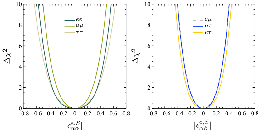
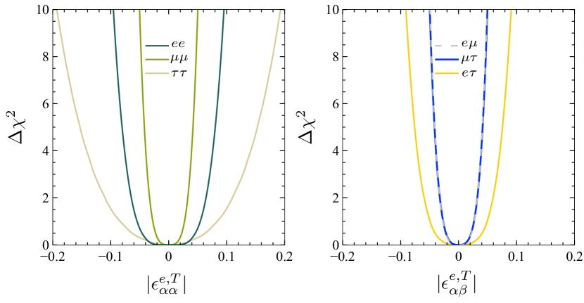
Figure 2: Global constraints on the neutrino-electron interaction parameters from different experiments. The upper (lower) panels correspond to the scalar (tensor) parameters. In the left (right) panels we present limits for the flavor-diagonal (changing) parameters.

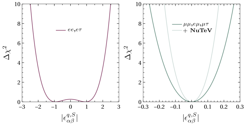
Figure 3: Global constraints on the neutrino-quark interaction parameters from different experiments. The upper (lower) panels correspond to the scalar (tensor) parameters. In the right panels we present the resulting limits without the NuTeV measurement (solid green line) and including it (solid gray line).

Experiments	Scalar	Pseudoscalar	Tensor
$e^{-}e^{+}$ + TEXONO	$|\epsilon^{e,S}_{ee}|<0.38$	$|\epsilon^{e,P}_{ee}|<0.40$	$|\epsilon^{e,T}_{ee}|<0.07$
$e^{-}e^{+}$ + CHARM-II	$|\epsilon^{e,X}_{\mu\mu}|<0.31$		$|\epsilon^{e,T}_{\mu\mu}|<0.03$
$e^{-}e^{+}$	$|\epsilon^{e,X}_{\tau\tau}|<0.40$		$|\epsilon^{e,T}_{\tau\tau}|<0.12$
$e^{-}e^{+}$ + TEXONO + CHARM-II	$|\epsilon^{e,S}_{e\mu}|<0.25$	$|\epsilon^{e,P}_{e\mu}|<0.25$	$|\epsilon^{e,T}_{e\mu}|<0.03$
$e^{-}e^{+}$ + TEXONO	$|\epsilon^{e,S}_{e\tau}|<0.28$	$|\epsilon^{e,P}_{e\tau}|<0.29$	$|\epsilon^{e,T}_{e\tau}|<0.07$
$e^{-}e^{+}$ + CHARM-II	$|\epsilon^{e,X}_{\mu\tau}|<0.25$		$|\epsilon^{e,T}_{\mu\tau}|<0.03$
CHARM$-e$	$|\epsilon^{q,X}_{ee}|<1.9$		$|\epsilon^{q,T}_{ee}|<0.13$
CHARM + CDHS (+ NuTeV)	$|\epsilon^{q,X}_{\mu\mu}|<0.15\,(0.1)$		$|\epsilon^{q,T}_{\mu\mu}|<0.01\,(0.006)$
CHARM$-e$ + CHARM + CDHS (+ NuTeV)	$|\epsilon^{q,X}_{e\mu}|<0.15\,(0.1)$		$|\epsilon^{q,T}_{e\mu}|<0.01\,(0.006)$
CHARM$-e$	$|\epsilon^{q,X}_{e\tau}|<1.9$		$|\epsilon^{q,T}_{e\tau}|<0.13$
CHARM + CDHS (+ NuTeV)	$|\epsilon^{q,X}_{\mu\tau}|<0.15\,(0.1)$		$|\epsilon^{q,T}_{\mu\tau}|<0.01\,(0.006)$

Table 6: Combined $90\%$ C.L. limits on the different scalar, pseudoscalar, and tensor neutrino interaction parameters, with $X=S,P$. For each suitable parameter, we also show in brackets the corresponding limits including the NuTeV measurements.

For completeness, we include an extra degree of freedom in this second part of the analysis, carrying out a new calculation where we let two parameters (of scalar and tensor nature) vary freely. Figs. 4 and 5 show the regions obtained at $90\%$ C.L. for neutrino-electron and neutrino-quark interactions. As expected, introducing an extra parameter relaxes the bounds on $\epsilon^{f,S}_{\alpha\beta}$ and $\epsilon^{f,T}_{\alpha\beta}$. Despite this, constraints coming from muon-neutrino-quark interactions are still the most restrictive as we can see in Fig. 5.

To conclude this section, we make a rough estimate of the scale for new physics implied by our constraints. As mentioned in the introduction, different models for new physics can lead to the couplings discussed here. To cite one example, models with leptoquarks, as the one discussed in Ref. Bischer and Rodejohann (2019b), could be an UV completion for GNI. If we consider the four-fermion effective interaction discussed here as the low energy limit of a heavy propagator coming from new physics, we will conclude that

$$\epsilon\frac{G_{F}}{\sqrt{2}}\simeq\frac{g_{X}^{2}}{M_{X}^{2}}\,,$$ (55)

where $g_{X}$ and $M_{X}$ are the coupling and mass of a new physics mediator, respectively. In this case, for neutrino-lepton interactions, our constraints will imply that $\frac{M_{X}}{g_{X}}\approx 550$ GeV for the scalar coupling and $\frac{M_{X}}{g_{X}}\approx 1.8$ TeV for the tensor case. For the neutrino-quark interactions, we will have $\frac{M_{X}}{g_{X}}\approx 1$ TeV for the scalar coupling and $\frac{M_{X}}{g_{X}}\approx 3.5$ TeV for the tensor case. These results are comparable with the ratios for $M_{X}/g_{X}$ presented in Bischer and Rodejohann (2019a) and are of the same order than in the charged-current sector (see, for example, Refs. Chang et al. (2015) and Gonzàlez-Solís et al. (2020)).

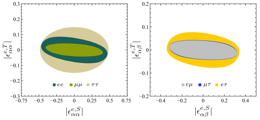
Figure 4: Global constraints on the scalar and tensor neutrino-electron parameters, at $90\%$ C.L. The same combination of experiments as in Table 6 was used. The left (right) panel shows the constraints on the diagonal (nondiagonal) parameters.

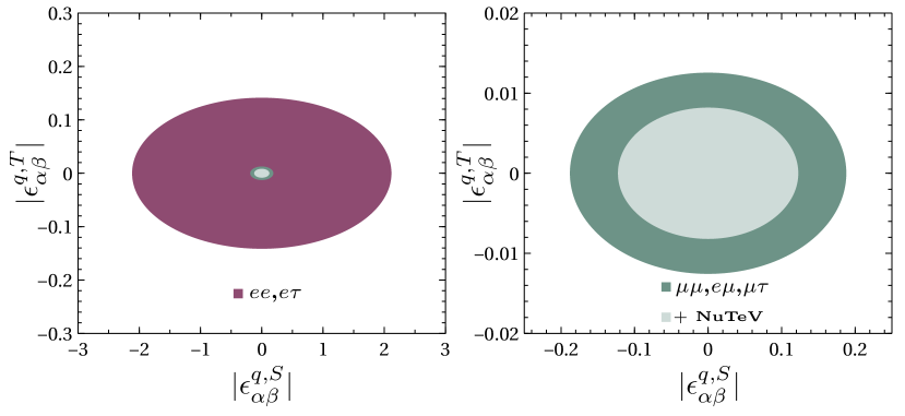
Figure 5: Global constraints on the scalar and tensor neutrino-quark parameters, at $90\%$ C.L. The same combination of experiments as in Table 6 was used. In the left panel we show the less stringent constraints corresponding to the parameters with flavor index $ee$ and $e\tau$. The other constraints, with and without including data from NuTeV, are presented in the right panel. As a reference for the reader, we also include the stronger constraints in the left panel.

V Conclusions

In this article, we have studied Generalized Neutrino Interactions in a model-independent way, following an effective field theory approach with the Standard Model theory at low energies as a framework. Based on a wide range of experimental results, we have performed a statistical analysis to find the restrictions on the different GNI parameters, especially for those of scalar, pseudoscalar, and tensor nature. For the sake of completeness, for vector and axial cases, we have quoted previously reported results.

We have studied the individual constraints for each of the nine experiments commented on previously. Some of these constraints are new, such as those coming from the electron-positron collision to a neutrino-antineutrino pair plus photon signal, the CDHS experiment, and the TEXONO experiment. We have also re-analyzed the NuTeV anomaly considering the recent results on the systematic uncertainties and provided new restrictive constraints for the GNI parameters. For the scalar and pseudoscalar cases, we have found that the bounds coming from the electron-positron collision experiments are of the same order of magnitude as those obtained from CHARM-II and TEXONO. In constrast, there is one order of magnitude difference for the tensor parameters.

We have also performed a robust global analysis for GNI using nine different neutrino experiments: ALEPH, DELPHI, L3, OPAL, CHARM-II, TEXONO, CHARM, CDHS, and NuTeV. With this analysis, we have set new constraints on the GNI parameters that, in some cases, are more restrictive than previously reported bounds. Being a global analysis, we have also shown the restrictions for combinations of two parameters at a time. We have found that, in general, the interactions with quarks are more constrained than the ones with electrons.

VI Acknowledgments

We thank useful discussions with Danny Marfatia. The work of LJF is supported by a postdoctoral CONACYT grant, CONACYT CB2017-2018/A1-S-13051 (México) and DGAPA-PAPIIT IN107118/IN107621. OGM has been supported by the CONACYT grant A1-S-23238. The work of J. R. has been granted by his CONACYT scholarship.

Appendix A Parametrizations for GNI interactions

There are at least two different parametrizations for GNI interactions Bischer and Rodejohann (2019b). For completeness, we show the relation between them in this appendix. In this work we have used the so-called epsilon parametrization

$$\mathcal{L}^{NC}_{eff}=-\frac{G_{F}}{\sqrt{2}}\sum_{j=1}{\epsilon}^{f,j}_{\alpha\beta\gamma\gamma}(\bar{\nu}_{\alpha}\mathcal{O}_{j}\nu_{\beta})(\bar{f}_{\gamma}\mathcal{O}^{{}^{\prime}}_{j}f_{\gamma}),$$ (56)

where we have defined the corresponding operators and couplings in Table 1. Note that, although redundant, we have explicitly written the flavor index in $\epsilon$ and $f$, to have a clear comparison with the $C$ and $D$ coefficients. In works Aristizabal Sierra et al. (2018); Han et al. (2020) they used the CD parametrization which is given by the following Lagrangian

$$\mathcal{L}=-\frac{G_{F}}{\sqrt{2}}\sum_{a=S,P,V,A,T}(\bar{\nu}_{\alpha}\Gamma^{a}\nu_{\beta})(\bar{f}_{\gamma}\Gamma^{a}(C^{a}_{\alpha\beta\gamma\gamma}+\bar{D}^{a}_{\alpha\beta\gamma\gamma}i\gamma^{5})f_{\gamma})\,,$$ (57)

where the five possible independent combinations of Dirac matrices are given by

$$\Gamma^{a}\in\{1,i\gamma^{5},\gamma^{\mu},\gamma^{\mu}\gamma^{5},\sigma^{\mu\nu}\}\,.$$ (58)

The relations between the coefficients $C^{a}_{\alpha\beta\gamma\gamma}$ and $D^{a}_{\alpha\beta\gamma\gamma}\equiv\begin{cases}\bar{D}^{a}_{\alpha\beta\gamma\gamma}\,(a=S,P,T)\\ i\bar{D}^{a}_{\alpha\beta\gamma\gamma}\,(a=V,A)\\ \end{cases}$ and the ${\epsilon}^{f,j}_{\alpha\beta\gamma\gamma}$ couplings is given below:

$$\epsilon^{L}=\frac{1}{4}(C^{V}-D^{V}+C^{A}-D^{A}),$$

$$\epsilon^{R}=\frac{1}{4}(C^{V}+D^{V}-C^{A}-D^{A}),$$

$$\epsilon^{S}=\frac{1}{2}(C^{S}+iD^{P}),$$ (59)

$$-\epsilon^{P}=\frac{1}{2}(C^{P}+iD^{S}),$$

$$\epsilon^{T}=\frac{1}{4}(C^{T}-iD^{T}).$$

References

- Abi et al. (2020) B. Abi et al. (DUNE), Eur. Phys. J. C 80, 978 (2020), arXiv:2006.16043 [hep-ex] .
- Abe et al. (2015) K. Abe et al. (Hyper-Kamiokande Proto-), PTEP 2015, 053C02 (2015), arXiv:1502.05199 [hep-ex] .
- Ohlsson (2013) T. Ohlsson, Rept. Prog. Phys. 76, 044201 (2013), arXiv:1209.2710 [hep-ph] .
- Miranda and Nunokawa (2015) O. G. Miranda and H. Nunokawa, New J. Phys. 17, 095002 (2015), arXiv:1505.06254 [hep-ph] .
- Farzan and Tortola (2018) Y. Farzan and M. Tortola, Front. in Phys. 6, 10 (2018), arXiv:1710.09360 [hep-ph] .
- Dev (2019) Neutrino Non-Standard Interactions: A Status Report, Vol. 2 (2019) arXiv:1907.00991 [hep-ph] .
- Giunti and Studenikin (2015) C. Giunti and A. Studenikin, Rev. Mod. Phys. 87, 531 (2015), arXiv:1403.6344 [hep-ph] .
- Miranda et al. (2019) O. G. Miranda, D. K. Papoulias, M. Tórtola, and J. W. F. Valle, JHEP 07, 103 (2019), arXiv:1905.03750 [hep-ph] .
- Aristizabal Sierra et al. (2020) D. Aristizabal Sierra, R. Branada, O. G. Miranda, and G. Sanchez Garcia, JHEP 12, 178 (2020), arXiv:2008.05080 [hep-ph] .
- Buchmuller et al. (1987) W. Buchmuller, R. Ruckl, and D. Wyler, Phys. Lett. B 191, 442 (1987), [Erratum: Phys.Lett.B 448, 320–320 (1999)].
- Crivellin et al. (2020) A. Crivellin, D. Müller, and F. Saturnino, JHEP 06, 020 (2020), arXiv:1912.04224 [hep-ph] .
- Gargalionis and Volkas (2021) J. Gargalionis and R. R. Volkas, JHEP 01, 074 (2021), arXiv:2009.13537 [hep-ph] .
- Ge and Parke (2019) S.-F. Ge and S. J. Parke, Phys. Rev. Lett. 122, 211801 (2019), arXiv:1812.08376 [hep-ph] .
- Khan et al. (2020) A. N. Khan, W. Rodejohann, and X.-J. Xu, Phys. Rev. D 101, 055047 (2020), arXiv:1906.12102 [hep-ph] .
- Heurtier and Zhang (2017) L. Heurtier and Y. Zhang, JCAP 02, 042 (2017), arXiv:1609.05882 [hep-ph] .
- Huang et al. (2018) G.-y. Huang, T. Ohlsson, and S. Zhou, Phys. Rev. D 97, 075009 (2018), arXiv:1712.04792 [hep-ph] .
- Forastieri et al. (2019) F. Forastieri, M. Lattanzi, and P. Natoli, Phys. Rev. D 100, 103526 (2019), arXiv:1904.07810 [astro-ph.CO] .
- Escudero and Witte (2020) M. Escudero and S. J. Witte, Eur. Phys. J. C 80, 294 (2020), arXiv:1909.04044 [astro-ph.CO] .
- Venzor et al. (2021) J. Venzor, A. Pérez-Lorenzana, and J. De-Santiago, Phys. Rev. D 103, 043534 (2021), arXiv:2009.08104 [hep-ph] .
- Bischer and Rodejohann (2019a) I. Bischer and W. Rodejohann, Phys. Rev. D 99, 036006 (2019a), arXiv:1810.02220 [hep-ph] .
- Bischer and Rodejohann (2019b) I. Bischer and W. Rodejohann, Nucl. Phys. B 947, 114746 (2019b), arXiv:1905.08699 [hep-ph] .
- Han et al. (2020) T. Han, J. Liao, H. Liu, and D. Marfatia, JHEP 07, 207 (2020), arXiv:2004.13869 [hep-ph] .
- Li et al. (2020a) T. Li, X.-D. Ma, and M. A. Schmidt, JHEP 10, 115 (2020a), arXiv:2007.15408 [hep-ph] .
- Chen et al. (2021) Z. Chen, T. Li, and J. Liao, (2021), arXiv:2102.09784 [hep-ph] .
- Lindner et al. (2017) M. Lindner, W. Rodejohann, and X.-J. Xu, JHEP 03, 097 (2017), arXiv:1612.04150 [hep-ph] .
- Papoulias and Kosmas (2018) D. K. Papoulias and T. S. Kosmas, Phys. Rev. D 97, 033003 (2018), arXiv:1711.09773 [hep-ph] .
- Aristizabal Sierra et al. (2018) D. Aristizabal Sierra, V. De Romeri, and N. Rojas, Phys. Rev. D 98, 075018 (2018), arXiv:1806.07424 [hep-ph] .
- Li et al. (2020b) T. Li, X.-D. Ma, and M. A. Schmidt, JHEP 07, 152 (2020b), arXiv:2005.01543 [hep-ph] .
- Buchmuller and Wyler (1986) W. Buchmuller and D. Wyler, Nucl. Phys. B 268, 621 (1986).
- Grzadkowski et al. (2010) B. Grzadkowski, M. Iskrzynski, M. Misiak, and J. Rosiek, JHEP 10, 085 (2010), arXiv:1008.4884 [hep-ph] .
- del Aguila et al. (2009) F. del Aguila, S. Bar-Shalom, A. Soni, and J. Wudka, Phys. Lett. B 670, 399 (2009), arXiv:0806.0876 [hep-ph] .
- Aparici et al. (2009) A. Aparici, K. Kim, A. Santamaria, and J. Wudka, Phys. Rev. D 80, 013010 (2009), arXiv:0904.3244 [hep-ph] .
- Luo et al. (2020) X. Luo, W. Rodejohann, and X.-J. Xu, JCAP 06, 058 (2020), arXiv:2005.01629 [hep-ph] .
- Rodejohann et al. (2017) W. Rodejohann, X.-J. Xu, and C. E. Yaguna, JHEP 05, 024 (2017), arXiv:1702.05721 [hep-ph] .
- Ruiz (2017) R. Ruiz, Eur. Phys. J. C 77, 375 (2017), arXiv:1703.04669 [hep-ph] .
- Cai et al. (2018) Y. Cai, T. Han, T. Li, and R. Ruiz, Front. in Phys. 6, 40 (2018), arXiv:1711.02180 [hep-ph] .
- Alcaide et al. (2019) J. Alcaide, S. Banerjee, M. Chala, and A. Titov, JHEP 08, 031 (2019), arXiv:1905.11375 [hep-ph] .
- Biekötter et al. (2020) A. Biekötter, M. Chala, and M. Spannowsky, Eur. Phys. J. C 80, 743 (2020), arXiv:2007.00673 [hep-ph] .
- Mangano et al. (2006) G. Mangano, G. Miele, S. Pastor, T. Pinto, O. Pisanti, and P. D. Serpico, Nucl. Phys. B 756, 100 (2006), arXiv:hep-ph/0607267 .
- Du and Yu (2021) Y. Du and J.-H. Yu, JHEP 05, 058 (2021), arXiv:2101.10475 [hep-ph] .
- Davidson et al. (2003) S. Davidson, C. Pena-Garay, N. Rius, and A. Santamaria, JHEP 03, 011 (2003), arXiv:hep-ph/0302093 .
- Barranco et al. (2008) J. Barranco, O. G. Miranda, C. A. Moura, and J. W. F. Valle, Phys. Rev. D 77, 093014 (2008), arXiv:0711.0698 [hep-ph] .
- Escrihuela et al. (2011) F. J. Escrihuela, M. Tortola, J. W. F. Valle, and O. G. Miranda, Phys. Rev. D 83, 093002 (2011), arXiv:1103.1366 [hep-ph] .
- Bolanos et al. (2009) A. Bolanos, O. G. Miranda, A. Palazzo, M. A. Tortola, and J. W. F. Valle, Phys. Rev. D 79, 113012 (2009), arXiv:0812.4417 [hep-ph] .
- Deniz et al. (2010a) M. Deniz et al. (TEXONO), Phys. Rev. D 82, 033004 (2010a), arXiv:1006.1947 [hep-ph] .
- Gonzalez-Garcia et al. (2011) M. C. Gonzalez-Garcia, M. Maltoni, and J. Salvado, JHEP 05, 075 (2011), arXiv:1103.4365 [hep-ph] .
- Barate et al. (1998a) R. Barate et al. (ALEPH), Phys. Lett. B420, 127 (1998a), arXiv:hep-ex/9710009 [hep-ex] .
- Barate et al. (1998b) R. Barate et al. (ALEPH), Phys. Lett. B429, 201 (1998b).
- Heister et al. (2003) A. Heister et al. (ALEPH), Eur. Phys. J. C28, 1 (2003).
- Abreu et al. (2000) P. Abreu et al. (DELPHI), Eur. Phys. J. C17, 53 (2000), arXiv:hep-ex/0103044 [hep-ex] .
- Acciarri et al. (1997) M. Acciarri et al. (L3), Phys. Lett. B415, 299 (1997).
- Acciarri et al. (1998) M. Acciarri et al. (L3), Phys. Lett. B444, 503 (1998).
- Acciarri et al. (1999) M. Acciarri et al. (L3), Phys. Lett. B470, 268 (1999), arXiv:hep-ex/9910009 [hep-ex] .
- Ackerstaff et al. (1998) K. Ackerstaff et al. (OPAL), Eur. Phys. J. C2, 607 (1998), arXiv:hep-ex/9801024 [hep-ex] .
- Abbiendi et al. (1999) G. Abbiendi et al. (OPAL), Eur. Phys. J. C8, 23 (1999), arXiv:hep-ex/9810021 [hep-ex] .
- Abbiendi et al. (2000) G. Abbiendi et al. (OPAL), Eur. Phys. J. C18, 253 (2000), arXiv:hep-ex/0005002 [hep-ex] .
- Berezhiani and Rossi (2002) Z. Berezhiani and A. Rossi, Phys. Lett. B535, 207 (2002), arXiv:hep-ph/0111137 [hep-ph] .
- Forero and Guzzo (2011) D. V. Forero and M. M. Guzzo, Phys. Rev. D 84, 013002 (2011).
- Escrihuela et al. (2020) F. J. Escrihuela, L. J. Flores, and O. G. Miranda, Phys. Lett. B 802, 135241 (2020), arXiv:1907.12675 [hep-ph] .
- Nicrosini and Trentadue (1989) O. Nicrosini and L. Trentadue, Nucl. Phys. B318, 1 (1989).
- Hirsch et al. (2003) M. Hirsch, E. Nardi, and D. Restrepo, Phys. Rev. D67, 033005 (2003), arXiv:hep-ph/0210137 [hep-ph] .
- Hasert et al. (1973) F. J. Hasert et al. (Gargamelle Neutrino), Phys. Lett. B 46, 138 (1973).
- Reines et al. (1976) F. Reines, H. S. Gurr, and H. W. Sobel, Phys. Rev. Lett. 37, 315 (1976).
- Daraktchieva et al. (2005) Z. Daraktchieva et al. (MUNU), Phys. Lett. B 615, 153 (2005), arXiv:hep-ex/0502037 .
- Vidyakin et al. (1992) G. S. Vidyakin, V. N. Vyrodov, I. I. Gurevich, Y. V. Kozlov, V. P. Martemyanov, S. V. Sukhotin, V. G. Tarasenkov, E. V. Turbin, and S. K. Khakhimov, JETP Lett. 55, 206 (1992).
- Derbin et al. (1993) A. I. Derbin, A. V. Chernyi, L. A. Popeko, V. N. Muratova, G. A. Shishkina, and S. I. Bakhlanov, JETP Lett. 57, 768 (1993).
- Dorenbosch et al. (1986) J. Dorenbosch et al. (CHARM), Phys. Lett. B 180, 303 (1986).
- Allaby et al. (1987) J. Allaby et al. (CHARM), Z. Phys. C 36, 611 (1987).
- Blondel et al. (1990) A. Blondel et al., Z. Phys. C 45, 361 (1990).
- Zeller et al. (2002) G. Zeller et al. (NuTeV), Phys. Rev. Lett. 88, 091802 (2002), [Erratum: Phys.Rev.Lett. 90, 239902 (2003)], arXiv:hep-ex/0110059 .
- Zyla et al. (2020) P. A. Zyla et al. (Particle Data Group), PTEP 2020, 083C01 (2020).
- Erler and Su (2013) J. Erler and S. Su, Prog. Part. Nucl. Phys. 71, 119 (2013), arXiv:1303.5522 [hep-ph] .
- Vilain et al. (1993) P. Vilain et al. (CHARM-II), Phys. Lett. B 302, 351 (1993).
- Vilain et al. (1994) P. Vilain et al. (CHARM-II), Phys. Lett. B 335, 246 (1994).
- Deniz et al. (2010b) M. Deniz et al. (TEXONO), Phys. Rev. D 81, 072001 (2010b), arXiv:0911.1597 [hep-ex] .
- Huber (2011) P. Huber, Phys. Rev. C 84, 024617 (2011), [Erratum: Phys.Rev.C 85, 029901 (2012)], arXiv:1106.0687 .
- Mueller et al. (2011) T. Mueller et al., Phys. Rev. C 83, 054615 (2011), arXiv:1101.2663 .
- Bellini et al. (2011) G. Bellini et al., Phys. Rev. Lett. 107, 141302 (2011), arXiv:1104.1816 [hep-ex] .
- Bellini et al. (2012) G. Bellini et al. (Borexino), Phys. Rev. Lett. 108, 051302 (2012), arXiv:1110.3230 [hep-ex] .
- Bellini et al. (2014) G. Bellini et al. (BOREXINO), Nature 512, 383 (2014).
- Agostini et al. (2019) M. Agostini et al. (Borexino), Phys. Rev. D 100, 082004 (2019), arXiv:1707.09279 [hep-ex] .
- Agostini et al. (2020a) M. Agostini et al. (Borexino), Phys. Rev. D 101, 062001 (2020a), arXiv:1709.00756 [hep-ex] .
- Agostini et al. (2020b) M. Agostini et al. (BOREXINO), Nature 587, 577 (2020b), arXiv:2006.15115 [hep-ex] .
- Bentz et al. (2010) W. Bentz, I. C. Cloet, J. T. Londergan, and A. W. Thomas, Phys. Lett. B 693, 462 (2010), arXiv:0908.3198 [nucl-th] .
- Jonker et al. (1981) M. Jonker et al. (CHARM), Phys. Lett. B 99, 265 (1981), [Erratum: Phys.Lett.B 100, 520 (1981), Erratum: Phys.Lett.B 103, 469 (1981)].
- Chang et al. (2015) H.-M. Chang, M. González-Alonso, and J. Martin Camalich, Phys. Rev. Lett. 114, 161802 (2015), arXiv:1412.8484 [hep-ph] .
- Gonzàlez-Solís et al. (2020) S. Gonzàlez-Solís, A. Miranda, J. Rendón, and P. Roig, Phys. Lett. B 804, 135371 (2020), arXiv:1912.08725 [hep-ph] .