The X-ray spectral and variability properties of typical radio-loud quasars

Abstract

We present X-ray spectral and long-term variability analyses of an unbiased sample of 361 optically selected radio-loud quasars (RLQs) utilizing sensitive serendipitous X-ray data from the Chandra and XMM-Newton archives. The spectral and temporal properties of RLQs are compared with those of radio-quiet quasars (RQQs) matched in $L_{\mathrm{2500\textup{\AA}}}$ and $z$. The median power-law photon index ($\Gamma$) of RLQs is $1.84_{-0.01}^{+0.01}$, which is close to that of matched RQQs ($1.90_{-0.01}^{+0.02}$). No significant correlations between $\Gamma$ and radio-loudness, $L_{\mathrm{x}}/L_{\mathrm{x,rqq}}$ (the X-ray luminosity over that expected from the $L_{\mathrm{x}}$-$L_{\mathrm{uv}}$ relation for RQQs), redshift, or Eddington ratio are found for our RLQs. The stacked X-ray spectra of our RLQs show strong iron-line emission and a possible Compton-reflection hump. The intrinsic X-ray variability amplitude is $\approx 40$% for RLQs on timescales of months-to-years in the rest frame, which is somewhat smaller than for the matched RQQs ($\approx 60$%) on similar timescales, perhaps due to the larger black-hole masses and lower Eddington ratios in our RLQ sample. The X-ray spectral and variability results for our RLQs generally support the idea that the X-ray emission of typical RLQs is dominated by the disk/corona, as is also indicated by a recent luminosity correlation study.

1 Introduction

Radio-loud quasars (RLQs) have powerful relativistic jets that are absent in radio-quiet quasars (RQQs; e.g. Padovani et al. 2017). These two types of quasars are observationally distinguished by the radio-loudness parameter, $R\equiv L_{\mathrm{5GHz}}/L_{\mathrm{4400\textup{\AA}}}$, where $L_{\mathrm{5GHz}}$ and $L_{\mathrm{4400\textup{\AA}}}$ are monochromatic luminosities at rest-frame 5 GHz and 4400 Å, respectively (Kellermann et al. 1989). Only 10–20% of quasars are RLQs with $R\geq 10$, while the rest are RQQs (e.g. Ivezić et al. 2002). Typical RLQs have similar near-infrared-to-UV spectral energy distributions (SEDs) to those of RQQs, showing the so-called big blue bump with strong emission lines superimposed (e.g. Elvis et al. 1994; Shang et al. 2011). However, RLQs are generally brighter X-ray emitters than RQQs and thus have a flatter optical/UV-to-X-ray spectral slope, $\alpha_{\mathrm{ox}}$ (e.g. Worrall et al. 1987; Miller et al. 2011), where $\alpha_{\mathrm{ox}}\equiv\log(L_{\mathrm{2keV}}/L_{\mathrm{2500\textup{\AA}}})/\log(\nu_{\mathrm{2keV}}/\nu_{\mathrm{2500\textup{\AA}}})$ assuming a power-law spectral shape between rest-frame 2 keV and 2500 Å (Tananbaum et al. 1979). Furthermore, the excess X-ray emission of RLQs above that of RQQs correlates with both $R$ and $L_{\mathrm{5GHz}}$, which has been taken as evidence that the nuclear X-ray emission of RLQs contains both a standard accretion-disk corona component as well as a distinct X-ray component associated with the base of the powerful radio jets (e.g. Worrall et al. 1987; Miller et al. 2011). This explanation seems consistent with some previous studies that have found that RLQs have systematically flatter X-ray ($<10$ keV) spectra than those of RQQs (e.g. Wilkes & Elvis 1987; Reeves et al. 1997; Page et al. 2005), which could arise due to the mixture of the coronal X-ray emission and a generally harder X-ray spectrum from the jet-linked emission (e.g. Grandi & Palumbo 2004).

This original two-component model of the nuclear X-ray emission from typical RLQs has recently been challenged by Zhu et al. (2020), who studied the correlations of the continuum emission from the corona, disk, and jets of RLQs. Zhu et al. (2020) investigated the correlations between X-ray, optical/UV, and radio luminosities using a large and well-characterized sample consisting of more than 700 optically-selected RLQs. The steep-spectrum radio quasars (SSRQs), which have a radio spectral slope $\alpha_{\mathrm{r}}\leq-0.5$, showed a $L_{\mathrm{x}}$-$L_{\mathrm{uv}}$ relation that is quantitatively similar to that of RQQs (i.e. $L_{\mathrm{x}}\propto L_{\mathrm{uv}}^{\gamma}$, $\gamma\approx$ 0.6; e.g. Just et al. 2007; Risaliti & Lusso 2019), despite the fact that these SSRQs are typically a factor of $\approx 2$–3 times more X-ray luminous than RQQs at a given $L_{\mathrm{uv}}$. The quantitatively similar $L_{\mathrm{x}}$-$L_{\mathrm{uv}}$ correlation for SSRQs supports the idea that the nuclear X-ray emission of these SSRQs is still dominated by the corona that is coupled with the accretion disk (e.g. Arcodia et al. 2019), and no jet component is required. Zhu et al. (2020) also showed that the jet-linked component is only important for a small fraction ($<10\%$) of flat-spectrum radio quasars (FSRQs; $\alpha_{\mathrm{r}}>-0.5$); thus, the corona-linked component also dominates the X-ray emission of most typical FSRQs. The relation between $\alpha_{\mathrm{ox}}$ and the equivalent width (EW) of He ii in RLQs is consistent with the result of Zhu et al. (2020) that RLQ X-ray emission is mainly related to the disk/corona instead of the jets (Timlin et al. 2021).

In light of these new results, it is important to investigate further the X-ray spectral properties of typical RLQs to assess whether they are indeed consistent with being mainly corona-linked. The primary X-ray continuum radiated from the hot corona is approximately described by a power law with a typical photon index of $\Gamma=1.7$–2.3 and an exponential cut-off at $\sim 100$ keV (e.g. Mushotzky et al. 1993; Kamraj et al. 2018; Molina et al. 2019), while the spectrum from the jets in the same band is a flatter power law ($\Gamma\sim 1.5$; e.g. Paliya et al. 2020) that might extend to $\gamma$-rays (e.g. Hartman et al. 1992). Kang et al. (2020) recently analyzed the NuSTAR spectra of 28 radio galaxies and detected the hard X-ray cut-off for 13 objects with sufficient net counts, which thus supports the idea that the hard X-rays of these radio galaxies are dominated by their coronae. Reprocessed X-ray emission can also be used to constrain the origin of the primary X-ray continuum. The iron emission lines between rest-frame 6.4–7.0 keV are of particular interest for this work, given their ubiquity in radio-quiet Seyfert galaxies (e.g. Nandra et al. 2007). If a beamed jet-linked continuum dominates the X-ray emission of RLQs, the iron-line emission is expected to be weak to undetectable owing to flux dilution (e.g. Reeves et al. 1997); otherwise, the corona-dominated interpretation for the X-ray emission of RLQs is favored. The Compton-reflection hump that broadly peaks at rest-frame 20–30 keV is also consistently expected if strong iron lines are detected (e.g. George & Fabian 1991).

Previous X-ray spectral studies of RLQs have often used small, heterogeneously-selected samples that might be biased. For example, previous RLQs selected in the radio band usually contain a significant portion of extreme FSRQs that have prominent jet-linked X-ray emission (see § 2 for further discussion). In this paper, we focus on the X-ray spectral properties of a large and optically selected RLQ sample (e.g. Zhu et al. 2020). Furthermore, we use only serendipitously obtained X-ray data to reduce potential selection effects caused by targeted X-ray observations (see § 2.1).

Further insights into the nature of the X-ray emission of RLQs can also be obtained by studying their X-ray variability properties, in comparison with those of RQQs. Generally, the X-ray variability properties of RLQs have only been investigated for either individual objects (e.g. Leighly et al. 1997; Hayashida et al. 2015) or small samples (e.g. Zamorani et al. 1984; Sambruna 1997; Gibson & Brandt 2012) rather than for large, homogeneous, statistically meaningful samples. In this work, we thus also investigate the X-ray variability properties of the typical RLQs selected by Zhu et al. (2020). See § 2.1 for the improvements of our sample relative to past work.

The sample construction and X-ray data analysis are discussed in § 2. The method used to fit the X-ray spectra and the fitting results are reported in § 3, and the long-term X-ray variability of RLQs is discussed in § 4. We adopt a $\Lambda$CDM cosmology with $H_{0}=70$ km s^-1 Mpc^-1 and $(\Omega_{\Lambda},\Omega_{\mathrm{M}})=(0.7,0.3)$.

2 Quasar Samples and X-ray Data Analysis

2.1 RLQ sample

Zhu et al. (2020) constructed a sample of 729 RLQs, utilizing the Sloan Digital Sky Survey (SDSS; York et al. 2000), the Faint Images of the Radio Sky at Twenty-Centimeters (FIRST; Becker et al. 1995), and the NRAO VLA Sky Survey (NVSS; Condon et al. 1998). These 729 quasars were initially selected using SDSS colors and are therefore not biased by their X-ray or radio properties. Archival Chandra, XMM-Newton, and ROSAT observations are used to calculate the X-ray luminosities of these optically-selected quasars. Only a small fraction ($\lesssim 15\%$) of the RLQ sample is targeted by these X-ray observations; therefore, this sample is not significantly biased by the target selection of these X-ray observations (e.g. Gibson & Brandt 2012). This RLQ sample also has large fractions of X-ray detections and spectroscopic confirmations by SDSS (see Table 1 of Zhu et al. 2020). Furthermore, almost all of the RLQs are classified as either FSRQs or SSRQs, utilizing radio surveys at frequencies other than 1.4 GHz, in particular, the Very Large Array Sky Survey (VLASS; Lacy et al. 2020) at $\approx 3$ GHz. Broad absorption line quasars, quasars that suffer from strong dust extinction, and quasars with prominent jet emission in the infrared-through-UV bands were excluded from this sample.

In order to investigate the X-ray temporal properties of RLQs using multiple-epoch observations, we match the RLQ list of Zhu et al. (2020) with the observation catalogs of Chandra and XMM-Newton. We only retain serendipitous observations (i.e. where the quasar position is $>1$ arcmin off-axis), which further minimizes the impacts of a small portion of RLQs in Zhu et al. (2020) that might be exceptional objects. The matching results in 326 Chandra/ACIS observations of 202 quasars and 474 XMM-Newton/EPIC observations of 293 quasars. The X-ray data reduction and quality cuts are described in the following subsections. Together, 333 RLQs will be used for X-ray spectral studies and 105 RLQs with more than one Chandra/XMM-Newton observation will be used to investigate the X-ray variability properties of RLQs. We list our final RLQ sample in Table 1 and X-ray observation sample in Table 2, respectively. The resulting RLQ sample in the luminosity-redshift plane is shown in Fig. 1.

We compare our spectral RLQ sample with those from previous investigations in Table 3, where the size of our RLQ sample is larger than those of previous samples by about one order of magnitude. Importantly, our RLQs are all optically selected quasars, while those previous samples are generally heterogeneous with a large portion that are radio selected, and the rest being optically or X-ray selected. Furthermore, all of our utilized X-ray observations were serendipitously observed, rendering our RLQ sample an unbiased subset of the optically selected SDSS quasars. In contrast, the previous samples usually utilized targeted X-ray observations, where the selection effects are hard to assess. Similarly, for our X-ray variability investigations, the sizes of the RLQ sample and X-ray observation sample are also significantly larger (by factors of $\approx 3$–100) than those in the literature, as reported in Table 4.

Table 1: The RLQ sample used in this paper. The quasar properties are taken from Zhu et al. (2020).

[b] Name $z$ $m_{i}$ $\log L_{\mathrm{2500\textup{\AA}}}$ $\log L_{\mathrm{5GHz}}$ $\log L_{\mathrm{2keV}}$ $\log R$ $\alpha_{\mathrm{r}}$ $\log(L_{\mathrm{x}}/L_{\mathrm{x,rqq}})$^a 000442.18$+$000023.3 1.008 18.91 30.22 32.08 26.91 1.74 - 0.56 000622.60$-$000424.4 1.038 19.51 30.04 34.94 27.31 4.76 $-$0.54 1.08 001646.54$-$005151.7 2.243 20.94 30.20 32.66 26.35 2.33 0.03 0.02 001910.95$+$034844.6 2.022 20.26 30.35 32.91 26.53 2.43 $-$0.75 0.10 003054.63$+$045908.4 2.201 20.92 30.18 33.81 26.59 3.49 $-$0.57 0.26

• The X-ray luminosity divided by that predicted by the $L_{\mathrm{x}}-L_{\mathrm{uv}}$ relation for RQQs (Zhu et al. 2020).

Table 2: The sample of RLQ X-ray observations.

[b] Name ObsID MJD^a Inst.^b $\log f_{\mathrm{det}}$^c net^d SNR^e $\log f_{\mathrm{x}}$^f xdet^g $\Gamma$^h goodness-of-fitⁱ 000442.18$+$000023.3 0305751001 53714.8 MOS2 $-13.92$ 263.1 15.5 $-$12.59 1 2.00${}_{-0.19}^{+0.19}$ 132.8/152.7/14.7 000622.60$-$000424.4 4096 52853.3 ACIS $-13.74$ 220.8 14.4 $-$12.35 1 1.76${}_{-0.21}^{+0.22}$ 214.3/188.3/16.1 000622.60$-$000424.4 5617 53579.5 ACIS $-14.35$ 806.8 28.3 $-$12.21 1 1.69${}_{-0.10}^{+0.11}$ 241.9/235.4/19.8 001646.54$-$005151.7 0403760101 54076.0 pn $-13.98$ 12.9 2.6 $-$13.82 1 1.23${}_{-1.11}^{+1.48}$ 80.1/83.8/10.1 001646.54$-$005151.7 0403760701 54295.3 pn $-14.38$ 24.3 4.0 $-$13.91 1 2.37${}_{-0.75}^{+0.93}$ 78.3/88.7/10.7

• Observation start time.

• The instrument used for the observation: ACIS for Chandra observations and pn/MOS1/MOS2 for XMM-Newton observations.

• The detection flux limit in the 0.5–7 keV band at the position of the quasar on the detector. See § 2.3.

• The net source counts after subtracting expected background counts, $\mathrm{net}=s-b/k$, where $k$ is the background-to-source area ratio.

• The signal-to-noise ratio, $\mathrm{SNR}=\mathrm{net}/\sqrt{s+b/k^{2}}$.

• The energy flux in the 0.5–7 keV band if the the quasar is detected. Otherwise, the upper bound of the 90% confidence interval is given.

• If the quasar is detected in the X-ray observation, $\mathrm{xdet}=1$. Otherwise, $\mathrm{xdet}=0$.

• The power-law photon index derived from our spectral fitting. $\Gamma=-99$ is used for cases of non-detection.

• The goodness-of-fit of the spectral fitting, $cstat/\mathrm{E}_{cstat}/\mathrm{S}_{cstat}$, where $cstat$ is the statistic of the fit, and $\mathrm{E}_{cstat}$ and $\mathrm{S}_{cstat}$ are the expectation and standard deviation of $cstat$, respectively (Kaastra 2017). For example, if $(cstat-\mathrm{E}_{cstat})/\mathrm{S}_{cstat}>4$, the fitting result is disfavored at a $4\sigma$ significance level.

Table 3: Previous sample-based investigations of the X-ray spectral properties of RLQs.

[b] Sample Telescope No. of RLQs^a Radio/Opt^b FSRQ/SSRQ^c This paper ($\mathrm{SNR}>3$) XMM-Newton/Chandra 333 0/333 184/134^d Zhou & Gu (2020) Chandra 43 43/0 14/29 Grandi et al. (2006) BeppoSAX 22 17/5 16/6 Page et al. (2005) XMM-Newton 16 10/4^e - Reeves & Turner (2000) ASCA 35 33/2 - Sambruna et al. (1999) ASCA 5 5/0 - Lawson & Turner (1997) Ginga 18 17/1 10/5^f Reeves et al. (1997) ASCA 15 13/2 8/0^g Lawson et al. (1992) EXOSAT 18 12/6 12/6 Wilkes & Elvis (1987) Einstein 17 14/3 - Notes: We use only serendipitous X-ray observations to ensure that our RLQs form a representative subset of the parent sample (i.e. optically selected SDSS RLQs). In contrast, all previous investigations listed here used targeted X-ray observations, which may be subject to complex selection effects (except for Zhou & Gu 2020).

• We provide the number of luminous quasars in this column, and other types of radio-loud AGNs (i.e. broad- and narrow-line radio galaxies) are excluded.

• The number of quasars that are selected in the radio/optical band.

• We list the number of FSRQs/SSRQs if the relevant paper provides radio-spectral information. Zhou & Gu (2020) divide their RLQs into core-dominated and lobe-dominated classes, which we associate with FSRQs and SSRQs, respectively.

• The remaining 15 RLQs do not have radio slope measurements.

• There are two X-ray selected objects in Page et al. (2005).

• Lawson & Turner (1997) separate the three optically violent variables (OVVs) from other FSRQs.

• The remaining seven RLQs of Reeves et al. (1997) are either OVVs or Gigahertz-peaked spectrum (GPS) radio sources.

Table 4: Previous investigations of the long-term X-ray variability of RLQs.

[b] Sample No. of RLQs/Object Name No. of Observations No. of pairs Timescale^a Studies of ensemble X-ray variability This paper (Down-sampled) 105 297 314 1.7 years Gibson & Brandt (2012) (High-quality sample) 8 20 15 1 year Zamorani et al. (1984) 7 14 7 1 year Studies of individual objects Marscher et al. (2018) 3C 120 $\approx 110$ - 8.3 months Chatterjee et al. (2011) 3C 111 822 - 5.9 years Soldi et al. (2008)^b 3C 273 1036 - 31 years Marscher (2006) 3C 120 $\approx 550$ - 3 years Marscher et al. (2002) 3C 120 $\approx 190$ - 3 years McHardy et al. (1999) 3C 273 84 - 1.4 months Leighly et al. (1997) 3C 390.3 90 - 4.6 months Sambruna (1997)^c 0923+392 7 - 2 years 3C 345 6 - 3 years Notes: In this table we do not include the X-ray monitoring studies of blazars and related highly jet-dominated objects (e.g. Chatterjee et al. 2008).

• The median rest-frame timescale is reported for the ensemble studies, while the maximum rest-frame timescale is reported for individual studies.

• We consider the 5 keV light-curve of 3C 273 in Soldi et al. (2008).

• We do not include 3C 279 and 0208$-$512 in Sambruna (1997), of which the former is a blazar and the data of the latter span only 12 days.

2.2 Data reduction

The Chandra and XMM-Newton observations were reduced using the ciao (v4.12) and sas (v18.0.0) packages, respectively. The Chandra data were reprocessed using chandra_repro and the most recent caldb (v4.9.3). Background flares were then removed using deflare. From the reprocessed, flare-filtered event files, we create clean images in the 0.5–7 keV band. Source detection is then performed using wavdetect with a threshold of $10^{-6}$ to obtain a list of X-ray sources in the field of view (FOV). If a RLQ is detected (i.e. an X-ray source is found within 2 arcsec of the quasar position), the X-ray position will be used for the following analysis; otherwise, the optically-determined quasar position is used. Note that cases where the quasar position is near the detector edge (i.e. the quasar lies within 40 pixels from the edge), falls in a detector gap, or is near an X-ray luminous cluster are excluded from further analysis. An elliptical region that encloses 90 per cent of the counts at the position of the quasar is created using the marx (v5.5.0) package (see § 3.1 of Timlin et al. 2020). The background region is defined as an annulus that is centered at the quasar position, with inner and outer radii of 15 and 50 arcsec, respectively. X-ray sources detected in the background region are excluded from the background region or, in a few cases where the RLQ is in a crowded field, a nearby circular background region is used. The source spectrum and associated response files and background spectrum are extracted using the specextract tool.

The EPIC-pn and EPIC-MOS data from XMM-Newton observations were reprocessed and cleaned using epproc and emproc, respectively. We filtered background-flaring periods using espfilt. Clean images are produced using evselect, and source detection is then performed using edetect_chain. Similar to the Chandra observations, cases where the quasar position is near the detector edge (i.e. the source region defined below overlaps with the detector boundary), falls in a detector gap, or is near an X-ray luminous cluster are excluded. Furthermore, if the background flaring is consistently strong throughout the exposure, we exclude the observation entirely. The source region is defined by a circle centered at the quasar position (or the X-ray position if an X-ray source is found within 5 arcsec of the quasar position). The radius of the circle is determined by eregionanalyse to optimize the signal-to-noise ratio. The background region is chosen to be a source-free circular region on the same chip, with a radius of $\gtrsim 40$ arcsec. The source and background spectra are then extracted using evselect. The corresponding RMFs and ARFs are created using rmfgen and arfgen, respectively.

In total, we obtain 300 useful Chandra/ACIS spectra of 195 RLQs and 401 useful XMM-Newton/EPIC spectra of 258 RLQs All of the following analyses are uniformly performed utilizing the spectral and associated response files, regardless of the observatories and instruments. Note that the RLQs being analyzed here are generally consistent with being X-ray point sources. The extended X-ray jet emission from RLQs, if it is spatially resolved, typically contributes only 1–3% to the total X-ray flux being analyzed (e.g. Marshall et al. 2018; Schwartz et al. 2020), and thus we do not expect such emission to affect our X-ray spectral and variability analyses below materially. Pileup is generally not a concern for serendipitous X-ray data with large off-axis angles ($>1$ arcmin).

2.3 Calculating energy flux and detection flux limit

Using the instrumental response files of each observation, an energy conversion factor (ECF) that converts the number of net counts to 0.5–7 keV energy flux is derived using sherpa (v4.13, Burke et al. 2020). The spectral shape of the photons that enter the X-ray telescopes is assumed to be a Galactic absorption-modified power law with $\Gamma=1.8$. This method is similar to that adopted in the XMM-Newton serendipitous source catalog (e.g. Rosen et al. 2016) and the Chandra source catalog (e.g. Evans et al. 2019).

The background-region counts, $b$, and the source-region counts, $s$, are read from the source and background spectra. The source detection is performed using the binomial no-source probability

$$P_{\mathrm{B}}(X\geq s)=\sum_{X=s}^{b+s}\frac{(b+s)!}{b!s!}p^{X}(1-p)^{b+s-X},$$ (1)

which is the probability of observing a source-to-background counts ratio as extreme as $s/b$, assuming that the $b+s$ counts are produced by a uniformly distributed X-ray source, i.e., the background (e.g. Broos et al. 2007; Weisskopf et al. 2007; Xue et al. 2011). Here, $p=1/(1+k)$, and $k$ is the ratio of the background-to-source region area. Since the test is performed at the pre-specified positions of optically bright objects, the quasar is considered detected if $P_{\mathrm{B}}\leq 0.002$ (2.88 $\sigma$), and the 1$\sigma$ uncertainties (i.e. 68% confidence interval) of their net counts are calculated using the ciao aprates tool (e.g. Primini & Kashyap 2014). If the quasar is not detected, we instead calculate the 90% confidence interval using aprates and consider the upper bound as the upper limit of the net counts. The net counts (upper limit) is then converted to energy flux (upper limit of the energy flux) in the 0.5–7 keV band using the ECF.

A flux limit of each XMM-Newton/Chandra observation at the quasar position can be calculated by reversing the problem of source detection. We find the limiting value of $s$ (denoted $s_{\mathrm{det}}$) that satisfies the inequality

$$\sum_{X=s}^{b+s}\frac{(b+s)!}{b!s!}p^{X}(1-p)^{b+s-X}\leq 0.002,$$ (2)

searching through integers from $s=1$. Note that $s_{\mathrm{det}}$ depends only on $b$ and $k$. A detection flux limit (denoted $f_{\mathrm{det}}$) can then be derived from $s_{\mathrm{det}}$ and the ECF calculated above. We apply a uniform, unbiased cut of $f_{\mathrm{det}}\leq 3\times 10^{-14}$ erg cm^-2 s^-1 for all X-ray observations to ensure a high detection fraction. The resulting X-ray observations are listed in Table 2. Note that if multiple cameras (i.e. pn, MOS1, and MOS2) are operating during an XMM-Newton observation, we keep the data from the camera with the smallest $f_{\mathrm{det}}$ and ignore the rest.

In total, 641 X-ray observations of 361 RLQs passed the flux-limit cut, of which 12 RLQs (3.3%) are not detected in any epoch and thus are not considered in the following analysis. Our X-ray spectral (§ 3) and variability (§ 4) investigations each utilize a subset of the remaining 349 RLQs, which are detected at least once in 628 X-ray observations. The vast majority of these observations (98.7%) result in significant X-ray detections, and thus our results are not substantively affected by X-ray upper limits.

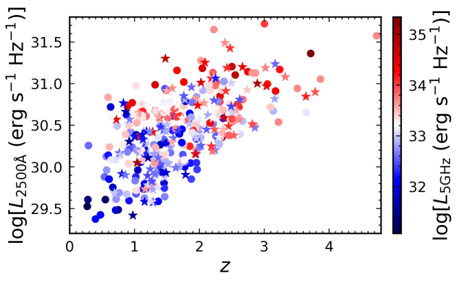
Figure 1: The distribution of RLQs from Zhu et al. (2020) with serendipitous Chandra/XMM-Newton observations in the $L_{\mathrm{2500\textup{\AA}}}-z$ plane. The stars and circles represent quasars having multiple X-ray observations or a single observation, respectively. The colors of the data points represent the radio luminosities as per the scale bar. Since the X-ray observations are serendipitous, these quasars span wide ranges in $L_{\mathrm{2500\textup{\AA}}}$, $L_{\mathrm{5GHz}}$, and $z$.

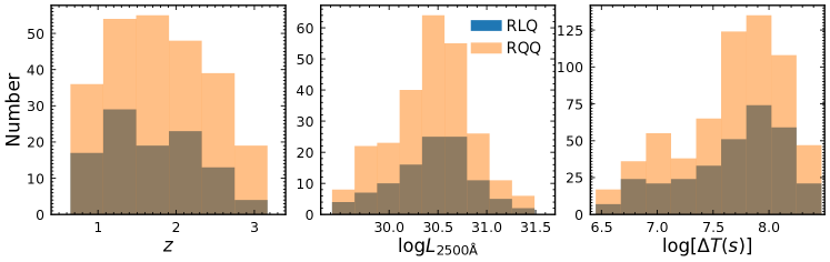
Figure 2: Comparisons of the matched RQQ and RLQ distributions of redshift, UV luminosity, and timescale (left, center, and right panels). The X-ray light-curves of the quasars in both samples have been down-sampled using the method in § 4.1. The RLQ and RQQ distributions in each parameter space are statistically consistent, according to AD tests of similarity for the three panels that all result in $p$-values $>0.16$.

2.4 Comparison RQQ sample

As part of this investigation, we will analyze the X-ray variability properties of our RLQ sample and require a suitable matched sample of RQQs with which we can compare our results. We select RQQs mainly from the sample of Timlin et al. (2020), who analyzed $\approx$ 1600 serendipitous Chandra X-ray observations of 462 typical, non-BAL RQQs. These spectroscopically-confirmed RQQs span a similar redshift range ($z=0.1$–4) to that of our RLQs (Fig. 1); however, Timlin et al. (2020) selected quasars with $m_{i}\leq 20.2$, which is about one magnitude brighter than the RLQs in our sample ($m_{i}\lesssim 21$). We therefore extended the analysis of Timlin et al. (2020) to fainter magnitude ($m_{i}=20.2$–20.8) quasars in the SDSS DR14Q (Pâris et al. 2018) following the selection method outlined in § 2 of Timlin et al. (2020). Note that all observations (including those from Timlin et al. 2020 and newly selected) are consistently analyzed in the same way as described above in § 2.2 and § 2.3. In total, we obtain 2341 serendipitous Chandra observations of 606 RQQs. We list the RQQ sample and corresponding X-ray observations in the tables presented in Appendix A.

Furthermore, to compare appropriately the long-term X-ray variability properties of RLQs with those of RQQs, we generated a sub-sample of RQQs that is matched in redshift, optical/UV luminosity, and timescale space to the RLQ sample. We describe the selection method in more detail in § 4.3. The redshift, optical/UV luminosity, and timescale distributions of the matched RQQs are compared with those of RLQs in Fig. 2. Note that two-sample Anderson-Darling (AD; Anderson & Darling 1952) tests are performed for all three panels of Fig. 2, and the distributions of RLQs and RQQs are always statistically consistent. We also selected a RQQ sample that matches with the RLQs used in § 3 as a reference for RQQ coronal X-ray spectral properties. To generate this sample, we selected the nearest RQQ in the $L_{\mathrm{2500\textup{\AA}}}$- $z$ space (without replacement) to each RLQ. An AD test indicates that the $L_{\mathrm{2500\textup{\AA}}}$ and $z$ distributions of this RQQ sample are statistically consistent with those of the RLQs used in § 3.

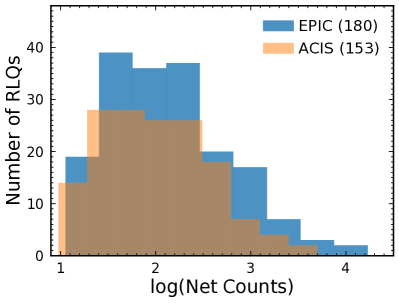
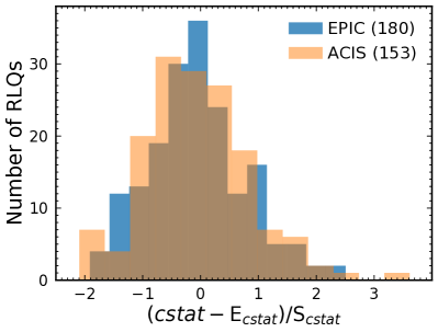
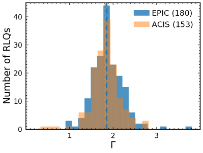
Figure 3: Top: The distribution of net counts (0.5–7 keV) of for the 333 RLQ X-ray spectra with SNR $\geq 3$, where (and in panels below) we distinguish the 153 Chandra/ACIS spectra from the remaining 180 XMM-Newton/EPIC spectra. Middle: The distribution of the quality of the spectral fits, $(cstat-\mathrm{E}_{cstat})/\mathrm{S}_{cstat}$. See the main text in § 3. Bottom: The distribution of $\Gamma$, where the median values are $1.82_{-0.01}^{+0.03}$ (dotted line) and $1.85_{-0.01}^{+0.02}$ (dashed line) for the ACIS and EPIC spectra, respectively.

3 X-ray Spectral Properties

We investigate the shape of the primary X-ray continuum in § 3.1 by fitting the X-ray spectra of individual quasars. The properties of X-ray reflection features, namely, the fluorescent iron line and the Compton hump, are analyzed in § 3.2, utilizing X-ray spectral stacking and joint spectral fitting.

3.1 Fitting the X-ray continuum using a power-law model

3.1.1 Fitting methods

We perform X-ray spectral fitting using sherpa, focusing on the observed-frame 0.5–7 keV band (rest-frame $0.55$–7.7 keV for quasars at $z\sim 0.1$ and 2.8–40 keV for quasars at $z\sim 4.5$). We use a simple power-law model to describe the shape of the quasar X-ray spectra, which is then multiplied by a $z=0$ absorption component with a fixed $N_{\mathrm{H}}$ value estimated using the colden tool (Dickey & Lockman 1990). The median number of counts between 0.5–7 keV of our X-ray spectra is 111, and the interquartile (25th to 75th percentile) range is (42, 289). Many X-ray spectra, therefore, do not have a sufficient number of counts to allow for further grouping, The c-stat statistic (denoted as $cstat$) is thus utilized, which provides maximum-likelihood estimates of model parameters without requiring a minimum number of counts in each bin/channel (Cash 1979; Baker & Cousins 1984; Humphrey et al. 2009).

When employing the c-stat statistic, the background contribution cannot be directly subtracted from the source spectrum; therefore, we fit the background spectra explicitly using empirical models. The background models are derived from principal component analysis using a larger number of background spectra of each instrument (i.e. ACIS, EPIC-pn, and EPIC-MOS; see Appendix A of Simmonds et al. 2018). After fitting the background spectra, the shape and amplitude of the background model is fixed, and a background component is added to the source model with a scaling factor (i.e. $1/k$; see § 2.3). The source spectra are then fitted with the full model that includes a Galactic absorption-modified power-law component (with two free parameters) and a fixed background component.

We assess the fit quality using the expectation and variance of the c-stat statistic of the best-fit model (Kaastra 2017).We denote the expectation and standard deviation of c-stat with $\mathrm{E}_{cstat}$ and $\mathrm{S}_{cstat}$, respectively. Ideally, the distribution of $(cstat-\mathrm{E}_{cstat})/\mathrm{S}_{cstat}$ is close to a standard normal distribution; in cases where $(cstat-\mathrm{E}_{cstat})/\mathrm{S}_{cstat}\gg 1$, the model is strongly disfavored. The X-ray spectra of RQQs are analyzed using the same methodology.

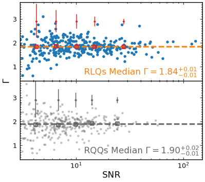
Figure 4: The best-fit power-law photon index ($\Gamma$) as a function of the SNR (see Table 2) of the spectrum for RLQs (top) and comparison RQQs (bottom). Both samples contain 333 quasars, and they are matched in $L_{\mathrm{2500\textup{\AA}}}$ and $z$. This figure demonstrates that the photon index does not depend on the quality of the data. The median photon index of all quasars in each panel is provided at the lower right corner. The RLQs are grouped into 5 SNR bins of nearly equal size (65–67 quasars per bin), and the median $\Gamma$ in each bin is calculated and shown as open squares. The uncertainties of the median $\Gamma$ of each bin are estimated using the bootstrapping method, and these uncertainties are relatively small compared with the size of the square symbols. Therefore, we additionally show the median uncertainties for individual sources in each bin above the squares. The binning scheme for RQQs follows that for RLQs. The X-ray spectra of RLQs are only flatter than those of RQQs by a small amount according to our serendipitous data.

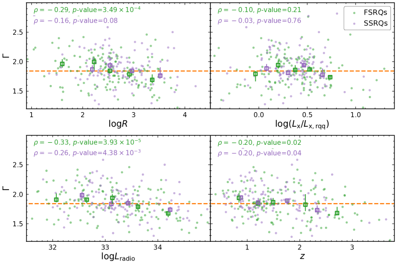
Figure 5: The correlations of photon index ($\Gamma$) with $\log R$, $L_{\mathrm{x}}/L_{\mathrm{x,rqq}}$, $L_{\mathrm{radio}}$, and $z$ for FSRQs (green symbols, 150 quasars) and SSRQs (purple symbols, 114 quasars), separately. Spectra with $\mathrm{SNR}\leq 5$ are omitted. The Spearman rank correlation statistic $\rho$ and the corresponding $p$-value are given at the upper-left corner of each panel. The median $\Gamma=1.84$ of the RLQ sample is shown in all four panels using orange dashed lines. In each panel, FSRQs and SSRQs are grouped into 5 and 4 bins of comparable size, respectively, according to their $x$-axis values. The median $\Gamma$ of each bin is calculated (open squares), the error bar of which is estimated using bootstrapping. There are no strong correlations ($p$-value $<10^{-3}$) between $\Gamma$ and $R$, $L_{\mathrm{x}}/L_{\mathrm{x,rqq}}$, $L_{\mathrm{radio}}$, and $z$ for FSRQs and SSRQs, except for the anti-correlation between $\Gamma$ and $L_{\mathrm{radio}}$ for FSRQs (lower left). A less significant anti-correlation between $\Gamma$ and $R$ for FSRQs (upper left) is probably driven by the $\Gamma$-$L_{\mathrm{radio}}$ anti-correlation for these FSRQs. However, if the 14 FSRQs with $\log L_{\mathrm{radio}}>34.3$ are removed, both anti-correlations disappear ($p$-value $>0.05$), suggesting that these FSRQs are the rare population of RLQs with a strong jet X-ray component and a flat photon index $\Gamma\sim$ 1.5–1.6. The lack of a correlation between $\Gamma$ and $\log(L_{\mathrm{x}}/L_{\mathrm{x,rqq}})$ argues against an important role of jet X-ray emission for general RLQs (e.g. Zhu et al. 2020). The photon index of the coronal X-ray component does not depend on the quasar properties under consideration here.

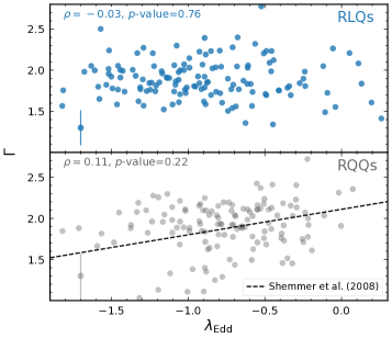
Figure 6: Top: The correlation between X-ray power-law photon index and Eddington ratio of RLQs. The median error bar of $\Gamma$ is shown in the lower-left corner. The Spearman rank correlation coefficient and associated $p$-value are shown in the upper-left corner. Bottom: Same as the top panel for comparison RQQs. The $\Gamma$-$\lambda_{\mathrm{Edd}}$ relation from Shemmer et al. (2008) is also shown for comparison. No strong correlation between $\Gamma$ and $\lambda_{\mathrm{Edd}}$ is found for either RLQs or RQQs.

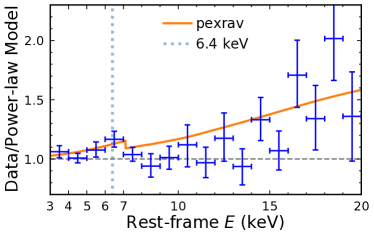
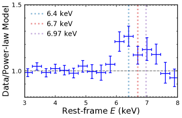
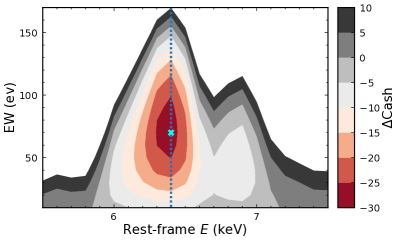
Figure 7: Top: The stacked ratio of the background-subtracted X-ray spectrum to the best-fit power-law model (with fixed $\Gamma=1.84$). We stacked the rest-frame 3–20 keV band using a bin size of 1 keV for the 58 RLQs with $z>2$ in our sample. The orange curve represents the prediction of Compton reflection from neutral material (i.e. pexrav, Magdziarz & Zdziarski 1995). Middle: The stacked data-to-model ratio in the rest-frame 3–8 keV band for 216 RLQs ($0.27<z<3.9$). Iron-line emission is clearly present in this residual spectrum. Bottom: The contour of the improvement of the fitting statistic ($\Delta$Cash) when a narrow emission line (a Gaussian profile with rest-frame FWHM $=20$ eV) is added to the power-law model (that is used in the top and middle panels). The cyan cross marks the minimum of the fitting statistic, where $\Delta$Cash$=-27.9$ indicates a 5.3$\sigma$ detection for a narrow iron line at 6.4 keV. The EW of the narrow iron line is $70_{-20}^{+30}$ eV.

3.1.2 The X-ray power-law photon indices of RLQs

In this section, we present fitting results for the X-ray spectra of 333 RLQs with SNR (i.e. signal-to-noise ratio) $\geq 3$ (16/349 RLQs fail this cut), where SNR $=3$ is approximately equivalent to a minimum number of 9 net counts between 0.5–7 keV. If a quasar has multiple observations, we utilize the X-ray spectrum from the observation with the smallest $f_{\mathrm{det}}$ and ignore the rest. The distribution of net counts for our RLQs is presented in the top panel of Fig. 3. In the middle panel of Fig. 3, we show the distribution of $(cstat-\mathrm{E}_{cstat})/\mathrm{S}_{cstat}$. There are 7 objects with $(cstat-\mathrm{E}_{cstat})/\mathrm{S}_{cstat}\geq 2$, which is consistent with the number expected from a standard normal distribution at $\geq 2\sigma$, i.e., $2.28\%\times 333\approx 7.6$. Therefore, our spectral-fitting results are generally acceptable, and the power-law model is a good phenomenological description of the rest-frame $\approx 0.5$–40 keV spectra of our RLQs. We show the distributions of $\Gamma$ of RLQs in Fig. 3 (bottom). The median $\Gamma$ for Chandra/ACIS and XMM-Newton/EPIC spectra are $1.82_{-0.01}^{+0.03}$ and $1.85_{-0.01}^{+0.02}$, respectively, where the uncertainties are estimated using bootstrapping. Therefore, any cross-calibration uncertainties between the instruments do not affect our results below.

We show the dependence of the resulting photon index $\Gamma$ on the SNR in Fig. 4 (top), where the orange dashed line represents the median $\Gamma$. The data points are also grouped into five equally-sized SNR bins, each of which contains $\approx 66$ spectra. The median $\Gamma$ values (as well as uncertainties derived using bootstrapping) of each bin are represented by red open squares with error bars in Fig. 4 (top). Since the error bars of each median $\Gamma$ are small compared to the symbol size, we also depict the median $\Gamma$ uncertainty for individual RLQs in each bin as the red error bars above the red squares. Fig. 4 shows no clear correlation between $\Gamma$ and SNR; thus, our methodology of X-ray spectral fitting is not sensitive to the data quality of the spectra. We repeat the procedure above for RQQs and show the results in Fig. 4 (bottom).

The median photon indexes of RLQs and matched RQQs are $1.84_{-0.01}^{+0.01}$ and $1.90_{-0.01}^{+0.02}$, respectively, the difference between which is small compared with the intrinsic spread of their $\Gamma$ distributions (0.19 and 0.25). The flat-spectrum and steep-spectrum RLQ subsets have median photon indexes of $1.84_{-0.02}^{+0.02}$ and $1.85_{-0.02}^{+0.04}$, respectively, the difference between which is small as well. However, in past work, the photon indexes of RLQs ($\Gamma\approx 1.5$–1.7) were often found to be significantly flatter than those of RQQs ($\Gamma\approx 1.7$–2.3; Wilkes & Elvis 1987; Reeves et al. 1997; Page et al. 2005), though this notable spectral difference was not always confirmed (e.g. Lawson et al. 1992; Sambruna et al. 1999; Grandi et al. 2006). Sambruna et al. (1999) found that the evidence is weak that broad-line radio galaxies (BLRGs) have flatter X-ray spectra than those of radio-quiet Seyfert 1 galaxies. Furthermore, previous studies that utilized RLQ samples containing SSRQs and treated them separately as a group (i.e. Lawson et al. 1992; Lawson & Turner 1997; Grandi et al. 2006) generally noticed a similarity between the photon indexes of SSRQs and those of RQQs. However, these studies had only a small number of SSRQs in their samples, which prevented solid conclusions from being drawn.

Zhu et al. (2020) found that the nuclear X-ray emission of RLQs is generally dominated by the corona, and the coronal X-ray luminosity depends on optical/UV luminosity and radio-loudness parameter, which indicate a disk-corona interplay and corona-jet connection, respectively. In Fig. 5, we investigate the correlations of the photon index of RLQs with other quasar properties. In particular, we are interested in testing if the corona-jet connection could affect, in addition to the X-ray brightness of the corona, the shape of the coronal X-ray spectrum. Specifically, correlations of the $\Gamma$ of coronal X-rays with $R$ and $L_{\mathrm{x}}/L_{\mathrm{x,rqq}}$ would provide insights into more details of the corona-jet connection. Even though Zhu et al. (2020) did not find a distinct jet X-ray component in SSRQs, the X-ray emission of a small portion ($\lesssim 10$%) of FSRQs likely contains a significant ($>30$%) jet X-ray component. We therefore treat FSRQs and SSRQs separately in Fig. 5, which is enabled by our large sample size. Furthermore, since statistical correlation analyses generally do not condsider the effects of measurement errors, we apply a cut of SNR $>5$ to the spectra to reduce the scatter caused by measurement errors, which results in 150 and 114 spectra of FSRQs and SSRQs, respectively, which are shown in Fig. 5.

We show the correlations of $\Gamma$ with $R$, $L_{\mathrm{x}}/L_{\mathrm{x,rqq}}$, $L_{\mathrm{radio}}$, and $z$ for FSRQs and SSRQs in Fig. 5. We perform Spearman rank-correlation tests and show the results in the upper-left corner of each panel. In addition, we group FSRQs and SSRQs into five and four bins of comparable size, respectively; the median $\Gamma$ is calculated for each bin and shown as large open squares in Fig. 5, the errors of which are estimated using bootstrapping. Neither the $p$-values resulting from correlation tests nor the median photon indexes support correlations (more significant than $p$-value $=10^{-3}$) between $\Gamma$ and $R$, $L_{\mathrm{x}}/L_{\mathrm{x,rqq}}$, $L_{\mathrm{radio}}$, and $z$ for SSRQs. No strong correlation is found for FSRQs either, except for the anti-correlation between $\Gamma$ and $L_{\mathrm{radio}}$ and a less-significant anti-correlation between $\Gamma$ and $R$; the latter correlation is probably driven by the former. There are 14 $\log L_{\mathrm{radio}}>34.3$ FSRQs in the lower-left panel of Fig. 5, almost all of which have $\Gamma$ that is smaller than the median photon index (1.84) of all RLQs. Instead, the photon indices of these most radio-luminous FSRQs are around 1.5–1.6. If these 14 FSRQs are removed in the correlation tests, the tentative $\Gamma$-$L_{\mathrm{radio}}$ and $\Gamma$-$R$ correlations disappear among the remaining 136 FSRQs. Therefore, these FSRQs likely represent the rare population that has a strong jet X-ray component (Zhu et al. 2020).

Finally, we matched the utilized RLQs and RQQs with the quasar-property catalog of Shen et al. (2011). There are 138 and 136 black-hole mass measurements (based on Mg ii or H$\beta$) for RLQs and RQQs, respectively. The median Eddington ratio of the RLQs ($-0.93_{-0.06}^{+0.04}$) is about $0.2$ dex smaller than that of the RQQs ($-0.73_{-0.06}^{+0.03}$), which might explain the mild difference between the median $\Gamma$ values of RLQs and RQQs if both groups follow the previously known correlation between $\Gamma$ and Eddington ratio (e.g. Shemmer et al. 2008; Brightman et al. 2013). However, a correlation between Eddington ratio and $\Gamma$ is not found for RLQs (see the top panel of Fig. 6), and a correlation test using Spearman’s $\rho$ results in $p$-value=0.76. A similar correlation test for the RQQ sample results in a negative result as well (see the bottom panel of Fig. 6), suggesting that our data quality might play an important role in the negative result for RLQs. Future RLQ samples with high-quality X-ray and infrared spectroscopy can address better the correlations between $\Gamma$ and Eddington ratio and FWHM of H$\beta$ (e.g. Brandt et al. 1997; Laor et al. 1997).

3.2 Iron-line emission and the Compton-reflection hump

The distribution of the fitting statistic in § 3.1.2 (i.e. the middle panel of Fig. 3) indicates that the power-law function is, globally, an acceptable description of the X-ray spectra of our individual RLQs; other features that arise in a narrow rest-frame X-ray band (e.g. fluorescent iron line emission) cannot be detected in individual spectra, given their limited numbers of counts. We therefore utilize a stacking technique to constrain the average properties of the fluorescent iron line and Compton reflection for our RLQs. We only consider RLQs with a spectroscopic redshift (83% of our sample) and an X-ray spectrum with SNR $>5$. We exclude 14 FSRQs with $\log L_{\mathrm{radio}}>34.3$ as these are potentially beamed objects (see § 3.1.2 and Fig. 5) and 2 other RLQs with $>10^{4}$ net counts since we do not want individual objects to dominate the spectral stacking, which results in 216 RLQ spectra for the analyses below. We first fit the individual X-ray spectra of RLQs using a power-law model with fixed $\Gamma=1.84$ (cf. § 3.1.2) excluding channels that correspond to the rest-frame $<2$ keV, 5–8 keV, and $>10$ keV bands, where additional emission features might exist. The single free parameter of the model, i.e., the normalization factor of the power-law function, is also fixed after fitting. For each X-ray spectrum, the data-to-model ratio is calculated over a grid of pre-defined rest-frame energy bins. Note that the background is subtracted from the total counts in each bin, and the model here refers to the Galactic absorbed power-law function. Finally, the data-to-model ratios of different RLQs are averaged in each energy bin.

We show the stacked data-to-model ratio over the rest-frame 3–20 keV band of 58 RLQs at $z>2$ (with a total of $7.4\times 10^{3}$ net counts) in the top panel of Fig. 7, where bins with a size of 1 keV are utilized. The error bars of each bin are estimated using bootstrapping. The data points that deviate from unity (the grey dashed line in the top panel of Fig. 7) show the locations where excess spectral features are present in the stacked residual spectrum. The vertical dotted line indicates the position (6.4 keV) of the fluorescent iron line expected from X-rays illuminating neutral material. The data between 6–7 keV signify that strong iron-line emission is present in the stacked spectrum. At $\geq 14$ keV, another strong feature is also apparent that might be associated with the Compton-reflection hump. We thus utilize the pexrav model (Magdziarz & Zdziarski 1995) of xspec to assess if the blue data points in Fig. 7 (top) are consistent with the prediction of Compton reflection for an X-ray source over a slab of neutral material. We choose a set of typical parameters, $\Gamma=1.84,E_{\mathrm{cut}}=300$ keV, and $\cos i=0.5$, with other parameters being set at their defaults. The resulting prediction is shown as the orange curve in Fig. 7 (top). The blue data points at $E>14$ keV generally follow the Compton-reflection model.

The middle panel of Fig. 7 shows the stacking results using all 216 RLQs over the rest-frame 2.95–8.05 keV band (with a total of $2.9\times 10^{4}$ net counts) with a bin size of 0.3 keV. We show the positions of rest-frame 6.4 keV, 6.7 keV, and 6.97 keV using vertical dotted lines. From this plot, it is apparent that the iron-line emission is not localized in a single bin but is distributed from $<6$ keV up to $>7$ keV, which cannot be explained by instrumental dispersion of a single narrow emission line. Possibly, both neutral and ionized material contributes to the iron-line production (e.g. Nandra et al. 1997), and Fig. 7 (middle) shows the blending of several narrow lines. Furthermore, since the excess emission also arises in the bin at $<6.4$ keV, a broad relativistic component is also likely present (e.g. Brenneman & Reynolds 2009).

To constrain the contribution from the narrow component of the neutral iron line at 6.4 keV, we utilize a method that is able to obtain the optimal energy resolution. We add a Gaussian function to the fixed power-law function to represent a narrow-line component for each quasar. The FWHM of the Gaussian function is fixed to be 20 eV in the rest frame, which is much smaller than the instrumental dispersion. The strength of the narrow emission line is parameterized using rest-frame EW. We sequentially increase the location of the narrow emission line from rest-frame 5.5 keV to 7.5 keV, with a step size of 0.1 keV. At each position, we iterate the EW of the line from 10 eV up to 200 eV, with a step size of 10 eV. The corresponding Cash statistic is calculated over the $21\times 20$ grid of line properties (i.e. location and strength). The Cash statistic of the simple power-law model without the narrow emission line is then subtracted, resulting in a two-dimensional $\Delta$Cash map for each quasar. We then summed the $\Delta$Cash maps of all quasars and show a contour plot of the results in Fig. 7 (bottom).

The minimum value in the contour plot, which corresponds to the largest improvement to the power-law model, occurs when the contour is at $E=6.4$ keV and EW $=70$ eV. The $\Delta$Cash value given these parameters is $\Delta$Cash $=-27.9$ and indicates that the neutral iron line is detected at a 5.3$\sigma$ significance level. The 90% confidence uncertainty of the EW is ($-20,+30$) eV, which corresponds to a change in $\Delta$Cash of 2.71. Hu et al. (2019) measured a strength of EW $\approx 50$ eV for a narrow emission line at 6.4 keV using the composite X-ray spectrum of 97 RL AGNs, which is consistent with our measurement within uncertainties. This method indicates that the strongest narrow component of the iron emission is located at $E=6.4$ keV; however, substantial emission remains in the stacked spectrum at rest-frame 6–7 keV. Integrating the data-to-model ratio over 6–7 keV reveals a total iron-line emission EW of $189_{-44}^{+49}$ eV, leaving EW $\approx 120$ eV to other iron species and the possible broad-line component. We discuss the implications of the strong iron-line emission in § 5. Similar analyses for the matched RQQs result in EW $=100_{-30}^{+20}$ eV for the narrow emission component at 6.4 keV. Thus, the EWs for RLQs and RQQs appear statistically consistent.

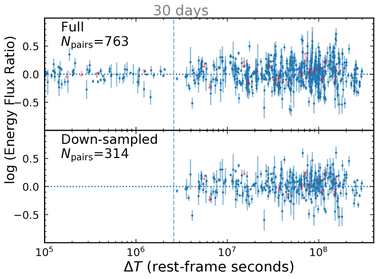
Figure 8: Energy flux ratio as a function of the rest-frame timescale, where the red downward and upward arrows represent upper and lower limits, respectively. The top panel shows all permutations of the full sample, while the bottom panel shows the permutations after removing repeated observations within 30 rest-frame days and down-sampling the X-ray data so that the number of observations of any RLQ is less than or equal to seven.

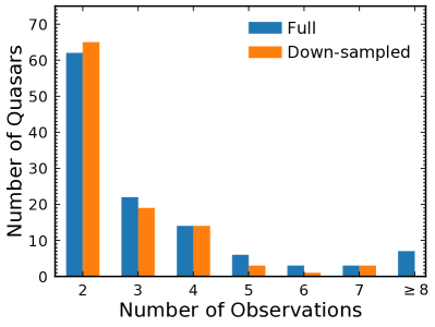
Figure 9: The number of X-ray observations for each RLQ in our variability study. The blue bars depict the 117 RLQs that have multiple Chandra/XMM-Newton observations with sensitivity better than $f=3\times 10^{-14}$ erg cm^-2 s^-1. The orange bars show the 105 RLQs remaining after removing repeated observations of the same RLQ within 30 days (in the rest frame) and down-sampling the X-ray data to reduce the maximum number of observations to seven per RLQ (see § 4.1).

4 Ensemble X-ray variability of RLQs

4.1 Energy flux ratio and down-sampling method

There are 117 RLQs in our sample that have more than one X-ray observation, and thus we are able to investigate, with a large set of data, how the X-ray brightness of these RLQs varies over time (in the quasar rest frame). For every pair of time-ordered data points in the X-ray light curve of a quasar in our sample, we calculate the ratio of the flux of the later-epoch data over that of the earlier epoch. For each of these energy flux ratios, there is a corresponding timescale (denoted $\Delta T$), which represents the time interval of the two observations corrected to the rest-frame of quasar. The dependence of energy flux ratio on the timescale is shown in the top panel of Fig. 8.

These 117 RLQs have 386 X-ray observations in total, where the number of observations of each quasar ranges from 2 to 20. The distribution of the number of observations of each quasar is shown as the blue bar plot in Fig. 9. For a quasar with $n$ X-ray observations, $n(n-1)/2$ energy flux ratios can be computed using the method outlined above. In Fig. 9, more than half of the quasars (65/117) have only two X-ray observations, resulting in 65 energy flux ratios; however, a single quasar with 20 X-ray observations produces 190 energy flux ratios. Therefore, to prevent the distribution of energy flux ratio from being dominated by a small number of quasars with a relatively large number of observations, we elect to down-sample the X-ray light curves. We first grouped any consecutive observations that are separated by <30 rest-frame days, and assigned each group an ID number. Among the observations with the same group ID, we keep only the most-sensitive observation (smallest $f_{\mathrm{det}}$), which removes 84 of the 386 observations. If the number of observations is still $>7$ after the grouping-and-selecting procedure above, we randomly remove observations (excluding the first and last ones to keep the maximum light-curve baseline) until only 7 observations remain, which removes 5 more observations. Note that if we down-sample the data to a maximum number of observations of 3, the main results of § 4 are not affected. The resulting distribution of the number of observations of each quasar is shown as the orange bars in Fig. 9, and the down-sampled energy flux ratio vs. rest-frame timescale is shown in the bottom panel of Fig. 8. The down-sampled data are used in the following analyses. After down-sampling the light-curves and restricting the timescale to $\Delta T\geq 30$ rest-frame days, 297 observations of 105 RLQs remained, producing 314 energy flux ratios (see Table 4).

4.2 X-ray variability of typical RLQs

We depict the distribution of the energy flux ratio in the top panel of Fig. 10 and the result of an AD normality test performed on the distribution of the energy fluxes in the first row of Table 5; the distribution does not depart significantly from a normal distribution. We calculated the kurtosis and estimated its uncertainties using bootstrapping. The kurtosis of the energy flux distribution for the RLQs is consistent with that of a normal distribution as well.

To remove the broadening of the distribution of energy flux ratio that is caused by measurement errors, and obtain the amplitude of the instrinsic X-ray variability, we fit a normal function to the distribution in Fig. 10 (top) using a maximum-likelihood method that distinguishes the measurement errors and intrinsic scatter (e.g. Maccacaro et al. 1988). The likelihood function includes terms that account for the few upper and lower limits in the data (e.g. see Appendix B of Zhu et al. 2019). The best-fit normal function that represents the intrinsic distribution of the energy flux ratio is shown as the orange curve in Fig. 10 (top), where the model parameters are presented in the upper-left corner.

To assess the dependence of X-ray variability amplitude on quasar luminosity and timescale, we divide the data at the median UV luminosity ($\log L_{\mathrm{2500\textup{\AA}}}=30.45$) and median timescale ($\log\Delta T=7.79$). We perform statistical tests on these sub-samples and report the results in Table 5. The distributions of energy flux ratio are consistent with a normal distribution in both luminosity and timescale bins. We also performed model fitting, as we did with the full sample, to the energy flux distributions of the luminosity and timescale bins and list the results in Table 6. There is strong evidence that the variability amplitude (i.e. $\sigma$) increases with rest-frame timescale (e.g. Timlin et al. 2020); however, the dependence of variability amplitude on quasar luminosity is only marginal.

Table 5: Statistical tests on distributions of energy flux ratio of RLQs.

[b] Sample $N_{\mathrm{pairs}}$ Normality ($p$-value)^a Kurtosis^b Down-sampled 314 0.02 $0.73_{-0.45}^{+0.38}$ High-luminosity ($\log L_{\mathrm{2500\textup{\AA}}}\geq 30.45$) 184 0.08 $0.66_{-0.43}^{+0.35}$ Low-luminosity ($\log L_{\mathrm{2500\textup{\AA}}}<30.45$) 130 0.45 $0.11_{-0.41}^{+0.31}$ Long-timescale ($\log\Delta T\geq 7.79$) 157 0.46 $0.35_{-0.37}^{+0.29}$ Short-timescale ($\log\Delta T<7.79$) 157 0.41 $0.27_{-0.47}^{+0.35}$

• The $p$-value resulting from the AD normality test.

• The kurtosis values do not strongly deviate from that of a normal distribution (kurtosis $=0$). The uncertainties of the kurtosis values are estimated using bootstrapping.

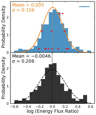
Figure 10: The distribution of $\log$(energy flux ratio) after down-sampling for RLQs is shown in the top panel, where red arrows represent upper/lower limits. The magnitude of the median measurement uncertainty is shown in the upper-right corner. The orange curve depicts the deconvolved normal function that represents the intrinsic variability. Note that the standard deviations of the distribution before and after deconvolution are 0.190 and 0.156, respectively. Therefore, the intrinsic variability dominates the spread of $\log$ (energy flux ratio). The mean and standard deviation of the intrinsic distribution are presented in the upper-left corner (orange). In the bottom panel, the distribution in black represents the matched RQQ sample with its respective deconvolved variability distribution (black dashed curve).

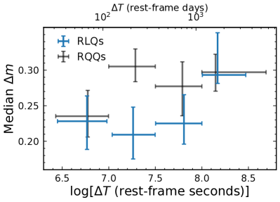
Figure 11: The ensemble structure function for the X-ray variability of RLQs (blue) compared with that of matched RQQs (black). The $x$-axis values are in units of both rest-frame seconds (bottom ticks) and days (top ticks). The X-ray variability amplitude of RQQs seems to be insensitive to timescale above $\approx 200$ rest-frame days. However, the structure function of RLQs apparently increases with $\Delta T$ out to the last bin, where RLQs become as variable as RQQs.

4.3 Comparing RLQs with matched RQQs

The energy flux ratios of RQQs are calculated and down-sampled following the method described in § 4.1. We then selected a matched sample of RQQs in the $z$, $\log L_{\mathrm{2500\textup{\AA}}}$, and $\log\Delta T$ parameter spaces. For each RLQs in the $z$-$\log L_{\mathrm{2500\textup{\AA}}}$-$\log\Delta T$ space, we select the two nearest RQQs, without replacement. We compare the distributions ($z$, $L_{\mathrm{2500\textup{\AA}}}$, and $\Delta T$) of matched RQQs in Fig. 2. AD tests are performed for the distributions in the three panels of Fig. 2, which support that the RQQs and RLQs are suitably matched.

We depict the energy flux ratio distribution of matched RQQs in the bottom panel of Fig. 10, where the black-dashed curve represents the normal function resulting from model fitting. Model fitting is also performed for sub-samples of RQQs divided by luminosity and timescale, and the results are summarized in Table 6. We find that, in our sample, the intrinsic X-ray variability amplitude of our RLQ sample is always smaller than that of the matched RQQ sample.

To further examine the dependence of X-ray flux variation on rest-frame timescale for the RLQ and RQQ samples, we calculate the often-utilized ensemble structure function (SF). We adopt the definition of SF from Fiore et al. (1998),

$$\Delta m_{ji}=\left|2.5\log[f(t_{j})/f(t_{i})]\right|,$$ (3)

where $f(t_{j})$ and $f(t_{i})$ are X-ray fluxes of individual objects that are measured at epochs $t_{j}$ and $t_{i}$ ($t_{j}>t_{i}$), respectively. Note that $\Delta m$ is equivalent to the absolute value of the previously computed energy flux ratio (Fig. 8) scaled by a factor of 2.5. We divide the data points into 4 timescale bins that are separated by $\Delta T=$ $10^{7}$, $10^{7.5}$, and $10^{8}$ s. These dividing points are chosen such that each bin evenly spans $\approx 0.5$ dex in timescale. The four bins contain 39, 59, 130, and 86 data points, respectively. The basic results are not affected if we merge the first 2 bins to make the distribution of data points in each bin more even. In each bin, the median value and uncertainties (estimated using bootstrapping) are calculated, and the typical (i.e. median) scatter caused by flux-measurement error is subtracted in quadrature, which has little effect on the shape but slightly decreases the amplitude of the SF. The SFs of RLQs and RQQs are shown in Fig. 11.

The SF of RQQs increases with $\Delta T$ in the first two bins; however, no significant increase is found at timescales above $\approx 200$ days. This result is consistent with Shemmer et al. (2017), who utilized a similar method and created an ensemble SF that increases at relatively short timescales and shows no substantial changes at relatively long timescales (see their Fig. 4). On the other hand, although the SF of RLQs is generally smaller than that of matched RQQs, it is consistent with increasing with $\Delta T$ out to the largest timescale bin, where the two types of quasars have similar variability amplitudes. The SF of RLQs is unconstrained at longer timescales and requires X-ray data with an extended baseline to test if a flattening occurs at $>3000$ days in the rest frame. (see § 6.2).

Table 6: Intrinsic variability distribution of RLQs compared with those of matched RQQs.

[b] Sample $m$^a $\sigma$^b RLQs RQQs RLQs RQQs Down-sampled $0.005_{-0.010}^{+0.010}$ $-0.004_{-0.009}^{+0.009}$ $0.156_{-0.007}^{+0.010}$ $0.212_{-0.007}^{+0.009}$ High-luminosity ($\log L_{\mathrm{2500\textup{\AA}}}\geq 30.45$) $0.016_{-0.014}^{+0.015}$ $-0.020_{-0.016}^{+0.016}$ $0.160_{-0.009}^{+0.015}$ $0.190_{-0.011}^{+0.015}$ Low-luminosity ($\log L_{\mathrm{2500\textup{\AA}}}<30.45$) $-0.007_{-0.014}^{+0.014}$ $0.004_{-0.012}^{+0.012}$ $0.150_{-0.010}^{+0.016}$ $0.208_{-0.009}^{+0.011}$ Long-timescale ($\log\Delta T\geq 7.79$) $-0.003_{-0.015}^{+0.016}$ $0.002_{-0.015}^{+0.015}$ $0.178_{-0.010}^{+0.016}$ $0.211_{-0.010}^{+0.014}$ Short-timescale ($\log\Delta T<7.79$) $0.014_{-0.013}^{+0.014}$ $-0.010_{-0.012}^{+0.013}$ $0.131_{-0.008}^{+0.014}$ $0.195_{-0.009}^{+0.012}$

• The mean of the deconvolved energy flux ratio distribution.

• The intrinsic variability amplitude after removing the contribution of the measurement errors.

5 Discussion

5.1 Comparison with previous sample-based X-ray spectral studies

X-ray observations of RLQs starting in the Einstein era have repeatedly found in sample-based studies (see § 2 and Table 1) that their X-ray continua below a few tens of keV (rest-frame) are significantly flatter than those of RQQs. The spectral-fitting results of our investigation, however, show that the median photon index of the X-ray spectra of our RLQ sample is $1.84_{-0.01}^{+0.01}$, which is significantly steeper than that obtained in previous studies ($\Gamma\sim 1.6$) and is found to be closer to that of the similarly selected RQQ sample ($1.90_{-0.01}^{+0.02}$). The median photon indexes of FSRQs and SSRQs are also consistent with each other. One of the main differences between our current work and previous investigations is that our work utilizes RLQs selected in SDSS color space whereas previous investigations mainly utilize radio-selected quasars. A bias was likely introduced when generalizing the high-energy properties of a small number of radio-selected RLQs to the full RLQ population in previous investigations. Radio surveys tend to select the most radio-luminous quasars in the Universe which may exhibit more extreme properties than their lower-luminosity counterparts which are included in optically selected RLQ samples (e.g. Kellermann et al. 1994; Gürkan et al. 2019). For example, the radio-selected FSRQs are generally considered to be beamed objects (e.g. Orr & Browne 1982), whereas most optically selected FSRQs seem to be an intermediate population between SSRQs and RQQs (e.g. Boroson & Green 1992; Falcke et al. 1996; Laor 2000), rather than highly beamed RLQs. Indeed, we find in the most radio-luminous regime ($\log L_{\mathrm{radio}}>34.3$) that FSRQs with flatter power-law slopes ($\Gamma~{}\sim 1.55$) dominate the population (see § 3.1.2). Additionally, it is risky to draw conclusions from sample-based studies that largely use targeted observations from archival X-ray data, since targeted objects have a poorly defined selection function and tend to have unique properties that are atypical of those of their parent population.

Siemiginowska et al. (2008) report the X-ray properties of a sample of RLQs that are also GPS and compact steep spectrum (CSS) radio sources. They measured a median photon index of $\Gamma=1.84$, which is consistent with our results and indicates that the X-ray spectral properties of GPS and CSS quasars are not necessarily different from those of typical RLQs.

5.2 The X-ray reflection features of RLQs

We detected strong iron K$\alpha$ emission in the rest-frame 6–7 keV band and a feature at rest-frame $>14$ keV that is likely the Compton-reflection hump in § 3.2. Such features are expected if the X-ray emission of RLQs is dominated by their coronae as for radio-quiet AGNs, where the evidence for iron-line emission is ubiquitous (e.g. Nandra et al. 2007). Iron-line emission can be detected from many radio-loud AGNs (e.g. Eracleous et al. 1996; Lohfink et al. 2017; Rani & Stalin 2018) but is not ubiquitously observed (e.g. Eracleous & Halpern 1998). The general consensus is that the X-ray reflection features of radio-loud AGNs generally seem to be weaker than those of radio-quiet AGNs (e.g. Wozniak et al. 1998; Eracleous et al. 2000), possibly due to dilution by a beamed X-ray continuum from jets (e.g. Ghisellini et al. 2019), an ionized accretion disk (e.g. Ballantyne et al. 2014), or an outflowing corona (e.g. King et al. 2017).

The iron-line emission from AGNs shows an X-ray Baldwin effect such that the EW of the narrow component of the neutral iron line decreases with increasing 2–10 keV luminosity (Iwasawa & Taniguchi 1993). This anti-correlation is significant for radio-quiet AGN samples (e.g. Bianchi et al. 2007; Shu et al. 2012), but it remains unclear if radio-loud AGNs follow the same relation. Typically, radio-loud AGNs are removed from such correlation studies since their supposed jet-linked X-ray emission can increase continuum X-ray luminosity, reduce the EW of iron line emission, and cause an artificial X-ray Baldwin effect (e.g. Jiménez-Bailón et al. 2005; Jiang et al. 2006). If the iron-line emission from our RLQs is produced by the primary X-ray continuum radiated from a RQQ-like corona and is then diluted by a jet-linked continuum (with an intensity comparable to that of the coronal component), we would expect a typical strength of EW $\approx 20$ eV (e.g. Eq. 1 in Bianchi et al. 2007), which is considerably weaker than the EW $=70_{-20}^{+30}$ eV that we found for our RLQ sample in § 3.2. If we instead consider the X-ray emission to be dominated by the corona, the EW we measure is still somewhat stronger than that predicted by the X-ray Baldwin effect (EW $\approx$ 40 eV). Possibly, a broad component contributes some amount of the emission at 6.4 keV due to limited energy resolution (especially at high redshift). Future X-ray missions with improved energy resolution and throughput can probe the details of the profile of the iron lines (see § 6.2). It is also possible that RLQs follow a different X-ray Baldwin relation from that of RQQs if the decrease of iron-line EW is related to but not directly caused by the increase of $L_{\mathrm{x}}$. For example, if the X-ray Baldwin effect is caused by a receding torus (e.g. Lawrence 1991; Simpson 2005) and the inner radius (and thereby the covering factor) of the torus is mainly determined by the UV luminosity, RLQs of similar radio-loudness will have a distinct EW-$L_{\mathrm{x}}$ relation. All in all, our investigation indicates that the iron-line emission of RLQs is not considerably diluted by a strong jet X-ray component.

The spectral shape and prominence of the iron line found in this work, along with our other measurements of X-ray spectral properties, put constraints on the model of the AGN corona. For example, a dynamic corona (e.g. Beloborodov 1999; Malzac et al. 2001) is used to explain the X-ray properties of AGNs in some studies (e.g. King et al. 2017). This model invokes a hot corona that moves away from the SMBH at a mildly relativistic velocity and is accelerated into the large-scale jet in radio-loud AGNs; the hot corona in radio-quiet AGNs is static or moves at a lower velocity. According to this model, the flatter X-ray continuum, lower level of X-ray reflection, and higher jet power of radio-loud AGNs are attributed to the higher outflow velocities of their coronae than those of radio-quiet AGNs. However, our spectral-fitting and X-ray spectral-stacking results do not support a substantial difference between the shapes of the X-ray continua of RLQs and RQQs or significantly weaker reflection in RLQs, and therefore rule out the idea that the outflow velocity of the corona is the key parameter controlling the X-ray and jet properties (e.g. Gupta et al. 2020).

5.3 The X-ray variability of RLQs

The typical X-ray variability amplitude of our optically selected RLQs on timescales of months-to-years in the rest frame is $\approx 40\%$, and extreme variations are rare in our data (see Fig. 8), which is not consistent with jet-dominated objects that show frequent large-amplitude flares in their X-ray light curves (e.g. Ulrich et al. 1997; Chatterjee et al. 2008; Castignani et al. 2017; Weaver et al. 2020). This qualitative similarity to the variability of RQQs (e.g. Timlin et al. 2020) may indicate that the X-ray emission of our RLQs is coronal-dominated. The overall variability amplitude is somewhat smaller than that of matched RQQs ($\approx$ 60%), and the X-ray variability amplitude increases with timescale, consistent with a red-noise-type power spectrum (e.g. Uttley & McHardy 2005). The fact that RLQs vary less than RQQs in the X-ray band at fixed timescale might suggest that RLQs require a relatively longer timescale to vary as much as RQQs, which is supported by the SFs depicted in Fig. 11.

Assuming that the fluctuations of the accretion flow propagate at similar speeds in both RQQs and RLQs, the timescale of flux variability then reflects the physical scale of the X-ray emitting region; the coronae of RLQs would be larger than those of matched RQQs. It is possible that the size of the corona is larger in RLQs than in RQQs at fixed black-hole mass (e.g. Dogruel et al. 2020). An anti-correlation between the X-ray variability amplitude and black-hole mass among radio-quiet AGNs is observed (e.g. O’Neill et al. 2005; Ponti et al. 2012). It is therefore also possible to consider a simpler scenario where the corona size scales with the black-hole mass similarly for both RLQs and RQQs, provided that the SMBHs of our RLQs are generally more massive than those of matched RQQs (e.g. Laor 2000). Indeed, there are 47 and 94 black-hole mass measurements (based on either Mg ii or H$\beta$) in the catalog of Shen et al. (2011) for the utilized RLQs and RQQs in our X-ray variability investigation, and the median black-hole mass of the RLQs is $\approx 0.2$ dex larger than that of the RQQs. Furthermore, the median Eddington ratio of the former group is $\approx 0.3$ dex smaller than that of the later, which might play an independent role as well (e.g. O’Neill et al. 2005). There is a characteristic timescale ($T_{\mathrm{B}}$) in the X-ray power spectrum of AGNs, above which the increase of the variability power per decade timescale is not as significant as below $T_{\mathrm{B}}$. This timescale depends on both the black-hole mass (e.g. Markowitz et al. 2003; Papadakis 2004) and Eddington ratio such that $T_{\mathrm{B}}\propto M_{\mathrm{BH}}/\lambda_{\mathrm{Edd}}$ (e.g. McHardy et al. 2006). Assuming that the X-ray power spectra of RLQs have a similar shape to those of radio-quiet AGNs and the characteristic timescale follows the same scaling relation above, the most significant increase of the X-ray variability amplitude of RLQs will occur at timescales $\approx 0.5$ dex larger than those of RQQs, which is roughly consistent with Fig. 11. To further assess the relation between black-hole mass/Eddington ratio and X-ray variability, we divide the 47 RLQs with measured black-hole masses into high-$M_{\mathrm{BH}}$/low-$\lambda_{\mathrm{Edd}}$ and low-$M_{\mathrm{BH}}$/high-$\lambda_{\mathrm{Edd}}$ groups at the median $M_{\mathrm{BH}}$ and found that the variability amplitude of the former group ($\sigma=0.15_{-0.01}^{+0.02}$) is significantly smaller than that of the later ($\sigma=0.22_{-0.02}^{+0.03}$), consistent with the assumption above.

Another possible explanation for the smaller variability amplitudes of RLQs is that the fluctuations of the inner accretion flow are relatively weak in RLQs compared to RQQs at fixed timescale. MacLeod et al. (2010) compared the optical/UV variability properties of quasars of different radio-loudness using SDSS Stripe 82 data. Except for the most radio-loud group that might be contaminated by jet emission in the optical/UV band, the variability amplitudes of moderately radio-loud quasars are slightly (but significantly) smaller than those of radio-nondetected quasars (with controlled black-hole mass, luminosity, and Eddington ratio). Cai et al. (2019) also suggest that the UV-emitting inner accretion flows of RLQs are stabilized (relative to those of RQQs) by the jet-launching magnetic field.

5.4 The $L_{\mathrm{x}}$-$L_{\mathrm{uv}}$-$L_{\mathrm{radio}}$ relation of RLQs

The X-ray spectral and variability properties obtained in this paper generally support the result of Zhu et al. (2020) that the X-ray emission of general RLQs is mainly radiated from their coronae. In particular, the lack of a strong correlation of $\Gamma$ with $L_{\mathrm{x}}/L_{\mathrm{x,rqq}}$ further disputes an important role of a jet X-ray component. Zhu et al. (2020) suggested that only in a small portion of FSRQs is the jet-linked X-ray component apparent. The parameterized model fitting in the correlation analyses in § 3.2 of Zhu et al. (2020) supports that both the coronal and jet X-ray components of FSRQs increase with radio luminosity such that $L_{\mathrm{x,corona}}\propto L_{\mathrm{radio}}^{0.2}$ (following the corona-jet connection, $L_{\mathrm{x,corona}}\propto R^{0.2}$) and $L_{\mathrm{x,jet}}\propto L_{\mathrm{radio}}$, predicting that the jet-linked X-ray component most clearly emerges in the most radio-luminous objects. Our spectral fitting results in § 3.1.2 (and the discussion above) of this paper are consistent with such a picture; in the most radio-luminous (likely beamed) FSRQs the jet core dominates the X-ray emission, resulting in significantly flattened X-ray spectra.

5.5 Connections with the hard X-ray emission of stellar-mass black holes

Several lines of evidence support a unification of the properties of the disk-corona/jet system surrounding accreting black holes spanning a wide range of mass (e.g. Merloni et al. 2003; McHardy et al. 2006; Körding et al. 2006; Zhu et al. 2020). Black-hole X-ray binaries (BHXRBs) usually show a high-energy cut-off and Compton reflection in their hard X-ray spectra (e.g. Gierlinski et al. 1997), similar to that of AGNs. Poutanen & Zdziarski (2003) pointed out that since the cut-off energy is always around several hundred keV, this feature is consistent with thermal Comptonization as well as a thermostat due to pair production but is not consistent with non-thermal synchrotron emission, the cut-off energy of which varies by large factors. Moreover, the reflection features are not consistent with the idea that the X-ray source is beamed away from the disk (Poutanen & Zdziarski 2003). The lack of abrupt changes during state transitions of BHXRBs is not expected if a radiatively inefficient jet dominates the X-ray emission (Maccarone 2005). Furthermore, the optical depth and temperature required by the jet-dominated model (e.g. Markoff et al. 2005) are often physically unrealistic (Malzac et al. 2009). There is sometimes a non-thermal tail that emerges in the MeV $\gamma$-ray spectra of BHXRBs (e.g. McConnell et al. 2002), which might come from a jet. However, this component is never energetically dominant in the X-ray band. Therefore, a jet-dominated model for the hard X-ray emission is disfavored for both accreting stellar-mass black holes and SMBHs, supporting unification ideas.

6 Summary and Future Prospects

6.1 Summary of main results

We present X-ray spectral and long-term variability analyses of a large sample of optically selected RLQs from Zhu et al. (2020). We utilize serendipitous X-ray data from the Chandra and XMM-Newton archives that are more sensitive than $3\times 10^{-14}$ erg cm^-2 s^-1 in the 0.5–7 keV energy band. The spectral and temporal properties of these RLQs are compared with those of matched RQQs (Timlin et al. 2020) using similarly selected X-ray data (see § 2 for details). The main results are summarized as follows:

1. The X-ray spectra of RLQs can be well described using a simple power-law model. From our model fits, we find the median photon index of RLQs is $1.84_{-0.01}^{+0.01}$, which is close to that of matched RQQs ($1.90_{-0.01}^{+0.02}$). The median photon indices are similar between FSRQs and SSRQs. We also investigated whether the $\Gamma$ values for FSRQs and SSRQs correlate with $R$, $L_{\mathrm{x}}/L_{\mathrm{x,rqq}}$, $L_{\mathrm{radio}}$, and $z$. No strong correlations are found. A small number of the most radio-luminous FSRQs ($\log L_{\mathrm{radio}}>34.3$), however, have flatter ($\Gamma\sim 1.55$) X-ray spectra than those of other RLQs. The stacked X-ray spectra of our RLQs show strong iron-line emission and a possible Compton-reflection hump. The narrow iron line at 6.4 keV is detected at a 5.3$\sigma$ significance level with EW = $70_{-20}^{+30}$ eV. See § 3.

2. We quantify the X-ray variability amplitude of the RLQs with multiple serendipitous observations. We required the interval between X-ray measurements to be larger than 30 days in the quasar rest frame; the median timescale is 1.7 year, and the longest timescale probed by our data is $\approx 10$ yr. Extreme large-amplitude variations are rare for our RLQs. The intrinsic variability amplitude after removing the scatter caused by measurement errors is $0.156_{-0.007}^{+0.010}$ (43.2%) for RLQs, which is significantly smaller than for the matched RQQs ($0.212_{-0.007}^{+0.009}$ or 62.9%) on similar timescales. The X-ray variability amplitude of RLQs increases with timescale, and the most significant increase occurs at longer timescales than for RQQs. See § 4.

3. The X-ray spectral (including the power-law photon index of the primary continuum and the strength of superimposed reflection features) and variability analyses of our RLQs support the results of Zhu et al. (2020) indicating that the X-ray emission of typical RLQs is dominated by the disk/corona. The previous claims that RLQs have substantially flatter X-ray spectra than those of RQQs are likely affected by various selection effects. Given the smaller variability amplitude of RLQs relative to RQQs matched in $L_{\mathrm{uv}}$, $z$, and timescale, the physical scale of the X-ray emitting region of the disk/corona system may be larger in RLQs, caused by their more massive SMBHs and/or lower Eddington ratio. A predominantly coronal origin for the X-ray emission of RLQs is also consistent with the results for the hard X-ray emission from stellar-mass black holes. See § 5.

6.2 Future work

Despite the notable connection between the X-ray brightness of the disk/corona and the jet efficiency of RLQs (Zhu et al. 2020), the basic spectral shape of the X-rays (i.e. $\Gamma$) radiated from the hot corona does not seem to be strongly affected by such a connection, demonstrated by the similarity between the median $\Gamma$ values of RLQs and RQQs and also by the fact that the $\Gamma$ values of individual RLQs do not seem to correlate with either $R$ or $L_{\mathrm{x}}/L_{\mathrm{x,rqq}}$. It therefore would be valuable to investigate how the physical properties of the corona (i.e. temperature, optical depth, and geometry) change with $R$ and $L_{\mathrm{x}}/L_{\mathrm{x,rqq}}$, which probably would require a powerful X-ray observatory with broadband response and excellent hard X-ray sensitivity (e.g. HEX-P; Harrison & HEX-P Collaboration 2017).

The next-generation X-ray observatories (e.g. Athena; Nandra et al. 2013) with orders of magnitude increases in effective area and energy resolution relative to current instruments will probe the iron emission lines and the Compton-reflection humps of individual RLQs, which can constrain the geometry and physical conditions of the material spiraling onto the black hole. Furthermore, it will be important to study if RLQs follow a similar $\Gamma$-$\lambda_{\mathrm{Edd}}$ relation as for RQQs.

The advent of eROSITA (Merloni et al. 2012) will produce copious well-sampled time-domain X-ray data that, when combined with existing archival data, will allow for better constraints upon the correlation between the variability amplitude of RLQs and timescale. X-ray variability is one of the most-promising methods that can constrain the physical scale of the quasar corona, and eROSITA measurements may allow testing of the variability scenarios described in § 5.3.

Data availability

The data used in this investigation are available in the article and in its online supplementary material.

Appendix A RQQ sample

The properties of the comparison RQQ sample (see the end of § 2.4) in this work are presented in Table 7. The serendipitous Chandra observations utilized for these RQQs, along with resulting derived X-ray properties, are listed in Table 8.

Table 7: The RQQ sample used in this paper.

[b] Name $z$ $m_{i}$ $\log L_{\mathrm{2500\textup{\AA}}}$ 000635.69$-$000721.04 0.891 20.65 29.47 002312.05$+$002545.99 2.657 20.64 30.48 002402.12$-$020101.13 2.614 19.90 30.77 002707.56$+$170617.88 0.947 20.25 29.69 002751.16$+$262437.66 1.173 20.40 29.77

Table 8: The sample of RQQ X-ray observations.

[b] Name ObsID MJD Inst. $\log f_{\mathrm{det}}$ net SNR $\log f_{\mathrm{x}}$ xdet $\Gamma$ goodness-of-fit 000635.69$-$000721.04 4096 52853.3 ACIS $-$14.02 3.1 1.5 $-$14.02 0 $-99$ 17.5/25.2/9.2 000635.69$-$000721.04 5617 53579.5 ACIS $-$14.13 32.4 4.8 $-$13.55 1 $2.06_{-0.58}^{+0.69}$ 116.5/128.7/13.6 002312.05$+$002545.99 2252 51915.4 ACIS $-$14.45 105.2 8.8 $-$13.11 1 $1.14_{-0.29}^{+0.31}$ 121.4/117.4/12.1 002402.12$-$020101.13 2099 52141.1 ACIS $-$14.53 9.6 3.0 $-$13.96 1 $2.04_{-0.90}^{+1.0}$ 40.6/47.4/11.2 002402.12$-$020101.13 8918 54768.1 ACIS $-$14.71 7.7 2.5 $-$14.39 1 $2.05_{-1.09}^{+1.48}$ 44.9/50.7/12.2 Notes: The columns of this table are similar to those of Table 2, where further explanations are provided.

References

- Anderson & Darling (1952) Anderson T. W., Darling D. A., 1952, Ann. Math. Statist., 23, 193
- Arcodia et al. (2019) Arcodia R., Merloni A., Nandra K., Ponti G., 2019, A&A, 628, A135
- Baker & Cousins (1984) Baker S., Cousins R. D., 1984, Nuclear Instruments and Methods in Physics Research, 221, 437
- Ballantyne et al. (2014) Ballantyne D. R., et al., 2014, ApJ, 794, 62
- Becker et al. (1995) Becker R. H., White R. L., Helfand D. J., 1995, ApJ, 450, 559
- Beloborodov (1999) Beloborodov A. M., 1999, ApJ, 510, L123
- Bianchi et al. (2007) Bianchi S., Guainazzi M., Matt G., Fonseca Bonilla N., 2007, A&A, 467, L19
- Boroson & Green (1992) Boroson T. A., Green R. F., 1992, ApJS, 80, 109
- Brandt et al. (1997) Brandt W. N., Mathur S., Elvis M., 1997, MNRAS, 285, L25
- Brenneman & Reynolds (2009) Brenneman L. W., Reynolds C. S., 2009, ApJ, 702, 1367
- Brightman et al. (2013) Brightman M., et al., 2013, MNRAS, 433, 2485
- Broos et al. (2007) Broos P. S., Feigelson E. D., Townsley L. K., Getman K. V., Wang J., Garmire G. P., Jiang Z., Tsuboi Y., 2007, ApJS, 169, 353
- Burke et al. (2020) Burke D., et al., 2020, sherpa/sherpa: Sherpa 4.12.1, doi:10.5281/zenodo.3944985, https://doi.org/10.5281/zenodo.3944985
- Cai et al. (2019) Cai Z., Sun Y., Wang J., Zhu F., Gu W., Yuan F., 2019, Science China Physics, Mechanics, and Astronomy, 62, 69511
- Cash (1979) Cash W., 1979, ApJ, 228, 939
- Castignani et al. (2017) Castignani G., et al., 2017, A&A, 601, A30
- Chatterjee et al. (2008) Chatterjee R., et al., 2008, ApJ, 689, 79
- Chatterjee et al. (2011) Chatterjee R., et al., 2011, ApJ, 734, 43
- Condon et al. (1998) Condon J. J., Cotton W. D., Greisen E. W., Yin Q. F., Perley R. A., Taylor G. B., Broderick J. J., 1998, AJ, 115, 1693
- Dickey & Lockman (1990) Dickey J. M., Lockman F. J., 1990, Annual Review of Astronomy and Astrophysics, 28, 215
- Dogruel et al. (2020) Dogruel M. B., Dai X., Guerras E., Cornachione M., Morgan C. W., 2020, ApJ, 894, 153
- Elvis et al. (1994) Elvis M., et al., 1994, ApJS, 95, 1
- Eracleous & Halpern (1998) Eracleous M., Halpern J. P., 1998, ApJ, 505, 577
- Eracleous et al. (1996) Eracleous M., Halpern J. P., Livio M., 1996, ApJ, 459, 89
- Eracleous et al. (2000) Eracleous M., Sambruna R., Mushotzky R. F., 2000, ApJ, 537, 654
- Evans et al. (2019) Evans I. N., et al., 2019, in AAS/High Energy Astrophysics Division. AAS/High Energy Astrophysics Division. p. 114.01
- Falcke et al. (1996) Falcke H., Patnaik A. R., Sherwood W., 1996, ApJ, 473, L13
- Fiore et al. (1998) Fiore F., Laor A., Elvis M., Nicastro F., Giallongo E., 1998, ApJ, 503, 607
- George & Fabian (1991) George I. M., Fabian A. C., 1991, MNRAS, 249, 352
- Ghisellini et al. (2019) Ghisellini G., et al., 2019, A&A, 627, A72
- Gibson & Brandt (2012) Gibson R. R., Brandt W. N., 2012, ApJ, 746, 54
- Gierlinski et al. (1997) Gierlinski M., Zdziarski A. A., Done C., Johnson W. N., Ebisawa K., Ueda Y., Haardt F., Phlips B. F., 1997, MNRAS, 288, 958
- Grandi & Palumbo (2004) Grandi P., Palumbo G. G. C., 2004, Science, 306, 998
- Grandi et al. (2006) Grandi P., Malaguti G., Fiocchi M., 2006, ApJ, 642, 113
- Gupta et al. (2020) Gupta M., Sikora M., Rusinek K., 2020, MNRAS, 492, 315
- Gürkan et al. (2019) Gürkan G., et al., 2019, A&A, 622, A11
- Harrison & HEX-P Collaboration (2017) Harrison F., HEX-P Collaboration 2017, in APS April Meeting Abstracts. p. K9.002
- Hartman et al. (1992) Hartman R. C., et al., 1992, ApJ, 385, L1
- Hayashida et al. (2015) Hayashida M., et al., 2015, ApJ, 807, 79
- Hu et al. (2019) Hu J., Liu Z., Jin C., Yuan W., 2019, MNRAS, 488, 4378
- Humphrey et al. (2009) Humphrey P. J., Liu W., Buote D. A., 2009, ApJ, 693, 822
- Ivezić et al. (2002) Ivezić Ž., et al., 2002, AJ, 124, 2364
- Iwasawa & Taniguchi (1993) Iwasawa K., Taniguchi Y., 1993, ApJ, 413, L15
- Jiang et al. (2006) Jiang P., Wang J. X., Wang T. G., 2006, ApJ, 644, 725
- Jiménez-Bailón et al. (2005) Jiménez-Bailón E., Piconcelli E., Guainazzi M., Schartel N., Rodríguez-Pascual P. M., Santos-Lleó M., 2005, A&A, 435, 449
- Just et al. (2007) Just D. W., Brandt W. N., Shemmer O., Steffen A. T., Schneider D. P., Chartas G., Garmire G. P., 2007, ApJ, 665, 1004
- Kaastra (2017) Kaastra J. S., 2017, A&A, 605, A51
- Kamraj et al. (2018) Kamraj N., Harrison F. A., Baloković M., Lohfink A., Brightman M., 2018, ApJ, 866, 124
- Kang et al. (2020) Kang J., Wang J., Kang W., 2020, ApJ, 901, 111
- Kellermann et al. (1989) Kellermann K. I., Sramek R., Schmidt M., Shaffer D. B., Green R., 1989, AJ, 98, 1195
- Kellermann et al. (1994) Kellermann K. I., Sramek R. A., Schmidt M., Green R. F., Shaffer D. B., 1994, AJ, 108, 1163
- King et al. (2017) King A. L., Lohfink A., Kara E., 2017, ApJ, 835, 226
- Körding et al. (2006) Körding E. G., Jester S., Fender R., 2006, MNRAS, 372, 1366
- Lacy et al. (2020) Lacy M., et al., 2020, PASP, 132, 035001
- Laor (2000) Laor A., 2000, ApJ, 543, L111
- Laor et al. (1997) Laor A., Fiore F., Elvis M., Wilkes B. J., McDowell J. C., 1997, ApJ, 477, 93
- Lawrence (1991) Lawrence A., 1991, MNRAS, 252, 586
- Lawson & Turner (1997) Lawson A. J., Turner M. J. L., 1997, MNRAS, 288, 920
- Lawson et al. (1992) Lawson A. J., Turner M. J. L., Williams O. R., Stewart G. C., Saxton R. D., 1992, MNRAS, 259, 743
- Leighly et al. (1997) Leighly K. M., O’Brien P. T., Edelson R., George I. M., Malkan M. A., Matsuoka M., Mushotzky R. F., Peterson B. M., 1997, ApJ, 483, 767
- Livesey (2007) Livesey J., 2007, Clinical biochemistry, 40, 1032
- Lohfink et al. (2017) Lohfink A. M., et al., 2017, ApJ, 841, 80
- MacLeod et al. (2010) MacLeod C. L., et al., 2010, ApJ, 721, 1014
- Maccacaro et al. (1988) Maccacaro T., Gioia I. M., Wolter A., Zamorani G., Stocke J. T., 1988, ApJ, 326, 680
- Maccarone (2005) Maccarone T. J., 2005, MNRAS, 360, L68
- Magdziarz & Zdziarski (1995) Magdziarz P., Zdziarski A. A., 1995, MNRAS, 273, 837
- Malzac et al. (2001) Malzac J., Beloborodov A. M., Poutanen J., 2001, MNRAS, 326, 417
- Malzac et al. (2009) Malzac J., Belmont R., Fabian A. C., 2009, MNRAS, 400, 1512
- Markoff et al. (2005) Markoff S., Nowak M. A., Wilms J., 2005, ApJ, 635, 1203
- Markowitz et al. (2003) Markowitz A., et al., 2003, ApJ, 593, 96
- Marscher (2006) Marscher A. P., 2006, Astronomische Nachrichten, 327, 217
- Marscher et al. (2002) Marscher A. P., Jorstad S. G., Gómez J.-L., Aller M. F., Teräsranta H., Lister M. L., Stirling A. M., 2002, Nature, 417, 625
- Marscher et al. (2018) Marscher A. P., et al., 2018, ApJ, 867, 128
- Marshall et al. (2018) Marshall H. L., et al., 2018, ApJ, 856, 66
- McConnell et al. (2002) McConnell M. L., et al., 2002, ApJ, 572, 984
- McHardy et al. (1999) McHardy I., Lawson A., Newsam A., Marscher A., Robson I., Stevens J., 1999, MNRAS, 310, 571
- McHardy et al. (2006) McHardy I. M., Koerding E., Knigge C., Uttley P., Fender R. P., 2006, Nature, 444, 730
- Merloni et al. (2003) Merloni A., Heinz S., di Matteo T., 2003, MNRAS, 345, 1057
- Merloni et al. (2012) Merloni A., et al., 2012, arXiv e-prints, p. arXiv:1209.3114
- Miller et al. (2011) Miller B. P., Brandt W. N., Schneider D. P., Gibson R. R., Steffen A. T., Wu J., 2011, ApJ, 726, 20
- Molina et al. (2019) Molina M., Malizia A., Bassani L., Ursini F., Bazzano A., Ubertini P., 2019, MNRAS, 484, 2735
- Mushotzky et al. (1993) Mushotzky R. F., Done C., Pounds K. A., 1993, ARA&A, 31, 717
- Nandra et al. (1997) Nandra K., George I. M., Mushotzky R. F., Turner T. J., Yaqoob T., 1997, ApJ, 488, L91
- Nandra et al. (2007) Nandra K., O’Neill P. M., George I. M., Reeves J. N., 2007, MNRAS, 382, 194
- Nandra et al. (2013) Nandra K., et al., 2013, arXiv e-prints, p. arXiv:1306.2307
- O’Neill et al. (2005) O’Neill P. M., Nandra K., Papadakis I. E., Turner T. J., 2005, MNRAS, 358, 1405
- Orr & Browne (1982) Orr M. J. L., Browne I. W. A., 1982, MNRAS, 200, 1067
- Padovani et al. (2017) Padovani P., et al., 2017, A&ARv, 25, 2
- Page et al. (2005) Page K. L., Reeves J. N., O’Brien P. T., Turner M. J. L., 2005, MNRAS, 364, 195
- Paliya et al. (2020) Paliya V. S., Ajello M., Cao H. M., Giroletti M., Kaur A., Madejski G., Lott B., Hartmann D., 2020, ApJ, 897, 177
- Papadakis (2004) Papadakis I. E., 2004, MNRAS, 348, 207
- Pâris et al. (2018) Pâris I., et al., 2018, A&A, 613, A51
- Ponti et al. (2012) Ponti G., Papadakis I., Bianchi S., Guainazzi M., Matt G., Uttley P., Bonilla N. F., 2012, A&A, 542, A83
- Poutanen & Zdziarski (2003) Poutanen J., Zdziarski A. A., 2003, in Durouchoux P., Fuchs Y., Rodriguez J., eds, New Views on Microquasars. p. 95 (arXiv:astro-ph/0209186)
- Primini & Kashyap (2014) Primini F. A., Kashyap V. L., 2014, ApJ, 796, 24
- Rani & Stalin (2018) Rani P., Stalin C. S., 2018, ApJ, 856, 120
- Reeves & Turner (2000) Reeves J. N., Turner M. J. L., 2000, MNRAS, 316, 234
- Reeves et al. (1997) Reeves J. N., Turner M. J. L., Ohashi T., Kii T., 1997, MNRAS, 292, 468
- Risaliti & Lusso (2019) Risaliti G., Lusso E., 2019, Nature Astronomy, 3, 272
- Rosen et al. (2016) Rosen S. R., et al., 2016, A&A, 590, A1
- Sambruna (1997) Sambruna R. M., 1997, ApJ, 487, 536
- Sambruna et al. (1999) Sambruna R. M., Eracleous M., Mushotzky R. F., 1999, ApJ, 526, 60
- Schwartz et al. (2020) Schwartz D. A., et al., 2020, ApJ, 904, 57
- Shang et al. (2011) Shang Z., et al., 2011, The Astrophysical Journal Supplement Series, 196, 2
- Shemmer et al. (2008) Shemmer O., Brandt W. N., Netzer H., Maiolino R., Kaspi S., 2008, ApJ, 682, 81
- Shemmer et al. (2017) Shemmer O., Brandt W. N., Paolillo M., Kaspi S., Vignali C., Lira P., Schneider D. P., 2017, ApJ, 848, 46
- Shen et al. (2011) Shen Y., et al., 2011, The Astrophysical Journal Supplement Series, 194, 45
- Shu et al. (2012) Shu X. W., Wang J. X., Yaqoob T., Jiang P., Zhou Y. Y., 2012, ApJ, 744, L21