Stateless Model Checking under a Reads-Value-From Equivalence

Abstract

Stateless model checking (SMC) is one of the standard approaches to the verification of concurrent programs. As scheduling non-determinism creates exponentially large spaces of thread interleavings, SMC attempts to partition this space into equivalence classes and explore only a few representatives from each class. The efficiency of this approach depends on two factors: (a) the coarseness of the partitioning, and (b) the time to generate representatives in each class. For this reason, the search for coarse partitionings that are efficiently explorable is an active research challenge.

In this work we present $\operatorname{RVF-SMC}$, a new SMC algorithm that uses a novel reads-value-from (RVF) partitioning. Intuitively, two interleavings are deemed equivalent if they agree on the value obtained in each read event, and read events induce consistent causal orderings between them. The RVF partitioning is provably coarser than recent approaches based on Mazurkiewicz and “reads-from” partitionings. Our experimental evaluation reveals that RVF is quite often a very effective equivalence, as the underlying partitioning is exponentially coarser than other approaches. Moreover, $\operatorname{RVF-SMC}$ generates representatives very efficiently, as the reduction in the partitioning is often met with significant speed-ups in the model checking task.

1 Introduction

The verification of concurrent programs is one of the key challenges in formal methods. Interprocess communication adds a new dimension of non-determinism in program behavior, which is resolved by a scheduler. As the programmer has no control over the scheduler, program correctness has to be guaranteed under all possible schedulers, i.e., the scheduler is adversarial to the program and can generate erroneous behavior if one can arise out of scheduling decisions. On the other hand, during program testing, the adversarial nature of the scheduler is to hide erroneous runs, making bugs extremely difficult to reproduce by testing alone (aka Heisenbugs[1]). Consequently, the verification of concurrent programs rests on rigorous model checking techniques [2] that cover all possible program behaviors that can arise out of scheduling non-determinism, leading to early tools such as VeriSoft [3, 4] and CHESS [5].

To battle with the state-space explosion problem, effective model checking for concurrency is stateless. A stateless model checker (SMC) explores the behavior of the concurrent program by manipulating traces instead of states, where each (concurrent) trace is an interleaving of event sequences of the corresponding threads [6]. To further improve performance, various techniques try to reduce the number of explored traces, such as context bounded techniques [7, 8, 9, 10] As many interleavings induce the same program behavior, SMC partitions the interleaving space into equivalence classes and attempts to sample a few representative traces from each class. The most popular approach in this domain is partial-order reduction techniques [11, 6, 12], which deems interleavings as equivalent based on the way that conflicting memory accesses are ordered, also known as the Mazurkiewicz equivalence [13]. Dynamic partial order reduction [14] constructs this equivalence dynamically, when all memory accesses are known, and thus does not suffer from the imprecision of earlier approaches based on static information. Subsequent works managed to explore the Mazurkiewicz partitioning optimally [15, 16], while spending only polynomial time per class.

The performance of an SMC algorithm is generally a product of two factors: (a) the size of the underlying partitioning that is explored, and (b) the total time spent in exploring each class of the partitioning. Typically, the task of visiting a class requires solving a consistency-checking problem, where the algorithm checks whether a semantic abstraction, used to represent the class, has a consistent concrete interleaving that witnesses the class. For this reason, the search for effective SMC is reduced to the search of coarse partitionings for which the consistency problem is tractable, and has become a very active research direction in recent years. In [17], the Mazurkiewicz partitioning was further reduced by ignoring the order of conflicting write events that are not observed, while retaining polynomial-time consistency checking. Various other works refine the notion of dependencies between events, yielding coarser abstractions [18, 19, 20]. The work of [21] used a reads-from abstraction and showed that the consistency problem admits a fully polynomial solution in acyclic communication topologies. Recently, this approach was generalized to arbitrary topologies, with an algorithm that remains polynomial for a bounded number of threads [22]. Finally, recent approaches define value-centric partitionings [23], as well as partitionings based on maximal causal models  [24]. These partitionings are very coarse, as they attempt to distinguish only between traces which differ in the values read by their corresponding read events. We illustrate the benefits of value-based partitionings with a motivating example.

1.1 Motivating Example

Consider a simple concurrent program shown in Figure 1. The program has 98 different orderings of the conflicting memory accesses, and each ordering corresponds to a separate class of the Mazurkiewicz partitioning. Utilizing the reads-from abstraction reduces the number of partitioning classes to 9. However, when taking into consideration the values that the events can read and write, the number of cases to consider can be reduced even further. In this specific example, there is only a single behaviour the program may exhibit, in which both read events read the only observable value.

Th $$\text{read}_{1}$$

$$1.\leavevmode\nobreak\ {\color[rgb]{0,0,0.8}w(x,1)}$$

$$2.\leavevmode\nobreak\ {\color[rgb]{0.8,0,0}w(y,1)}$$

Th $$\text{read}_{2}$$

$$1.\leavevmode\nobreak\ {\color[rgb]{0,0,0.8}w(x,1)}$$

$$2.\leavevmode\nobreak\ {\color[rgb]{0.8,0,0}w(y,1)}$$

$$3.\leavevmode\nobreak\ {\color[rgb]{0,0,0.8}r(x)}$$

Th $$\text{read}_{3}$$

$$1.\leavevmode\nobreak\ {\color[rgb]{0,0,0.8}w(x,1)}$$

$$2.\leavevmode\nobreak\ {\color[rgb]{0.8,0,0}w(y,1)}$$

$$3.\leavevmode\nobreak\ {\color[rgb]{0.8,0,0}r(y)}$$

Equivalence classe s:

Mazurkiewicz [15] $$98$$

reads-from [22] $$\;\>9$$

value-centric [23] $$\;\>7$$

this work $$\;\>1$$

Figure 1: Concurrent program and its underlying partitioning classes.

The above benefits have led to recent attempts in performing SMC using a value-based equivalence [24, 23]. However, as the realizability problem is NP-hard in general [25], both approaches suffer significant drawbacks. In particular, the work of [23] combines the value-centric approach with the Mazurkiewicz partitioning, which creates a refinement with exponentially many more classes than potentially necessary. The example program in Figure 1 illustrates this, where while both read events can only observe one possible value, the work of [23] further enumerates all Mazurkiewicz orderings of all-but-one threads, resulting in 7 partitioning classes. Separately, the work of [24] relies on SMT solvers, thus spending exponential time to solve the realizability problem. Hence, each approach suffers an exponential blow-up a-priori, which motivates the following question: is there an efficient parameterized algorithm for the consistency problem? That is, we are interested in an algorithm that is exponential-time in the worst case (as the problem is NP-hard in general), but efficient when certain natural parameters of the input are small, and thus only becomes slow in extreme cases.

Another disadvantage of these works is that each of the exploration algorithms can end up to the same class of the partitioning many times, further hindering performance. To see an example, consider the program in Figure 1 again. The work of [23] assigns values to reads one by one, and in this example, it needs to consider as separate cases both permutations of the two reads as the orders for assigning the values. This is to ensure completeness in cases where there are write events causally dependent on some read events (e.g., a write event appearing only if its thread-predecessor reads a certain value). However, no causally dependent write events are present in this program, and our work uses a principled approach to detect this and avoid the redundant exploration. While an example to demonstrate [24] revisiting partitioning classes is a bit more involved one, this property follows from the lack of information sharing between spawned subroutines, enabling the approach to be massively parallelized, which has been discussed already in prior works [21, 26, 23].

1.2 Our Contributions

In this work we tackle the two challenges illustrated in the motivating example in a principled, algorithmic way. In particular, our contributions are as follows.

1. We study the problem of verifying the sequentially consistent executions. The problem is known to be NP-hard [25] in general, already for 3 threads. We show that the problem can be solved in $O(k^{d+1}\cdot n^{k+1})$ time for an input of $n$ events, $k$ threads and $d$ variables. Thus, although the problem NP-hard in general, it can be solved in polynomial time when the number of threads and number of variables is bounded. Moreover, our bound reduces to $O(n^{k+1})$ in the class of programs where every variable is written by only one thread (while read by many threads). Hence, in this case the bound is polynomial for a fixed number of threads and without any dependence on the number of variables.

2. We define a new equivalence between concurrent traces, called the reads-value-from (RVF) equivalence. Intuitively, two traces are RVF-equivalent if they agree on the value obtained in each read event, and read events induce consistent causal orderings between them. We show that RVF induces a coarser partitioning than the partitionings explored by recent well-studied SMC algorithms  [15, 21, 23], and thus reduces the search space of the model checker.

3. We develop a novel SMC algorithm called $\operatorname{RVF-SMC}$, and show that it is sound and complete for local safety properties such as assertion violations. Moreover, $\operatorname{RVF-SMC}$ has complexity $k^{d}\cdot n^{O(k)}\cdot\beta$, where $\beta$ is the size of the underlying RVF partitioning. Under the hood, $\operatorname{RVF-SMC}$ uses our consistency-checking algorithm of Item 1 to visit each RVF class during the exploration. Moreover, $\operatorname{RVF-SMC}$ uses a novel heuristic to significantly reduce the number of revisits in any given RVF class, compared to the value-based explorations of [24, 23].

4. We implement $\operatorname{RVF-SMC}$ in the stateless model checker Nidhugg [27]. Our experimental evaluation reveals that RVF is quite often a very effective equivalence, as the underlying partitioning is exponentially coarser than other approaches. Moreover, $\operatorname{RVF-SMC}$ generates representatives very efficiently, as the reduction in the partitioning is often met with significant speed-ups in the model checking task.

2 Preliminaries

General notation. Given a natural number $i\geq 1$, we let $[i]$ be the set $\{1,2,\dots,i\}$. Given a map $f\colon X\to Y$, we let $\mathsf{dom}(f)=X$ denote the domain of $f$. We represent maps $f$ as sets of tuples $\{(x,f(x))\}_{x}$. Given two maps $f_{1},f_{2}$ over the same domain $X$, we write $f_{1}=f_{2}$ if for every $x\in X$ we have $f_{1}(x)=f_{2}(x)$. Given a set $X^{\prime}\subset X$, we denote by $f|X^{\prime}$ the restriction of $f$ to $X^{\prime}$. A binary relation $\sim$ on a set $X$ is an equivalence iff $\sim$ is reflexive, symmetric and transitive.

2.1 Concurrent Model

Here we describe the computational model of concurrent programs with shared memory under the Sequential Consistency ($\operatorname{SC}$) memory model. We follow a standard exposition of stateless model checking, similarly to [14, 15, 21, 22, 28, 23],

Concurrent program. We consider a concurrent program $\mathcal{H}=\{\mathsf{thr}_{i}\}_{i=1}^{k}$ of $k$ deterministic threads. The threads communicate over a shared memory $\mathcal{G}$ of global variables with a finite value domain $\mathcal{D}$. Threads execute events of the following types.

1. A write event $w$ writes a value $v\in\mathcal{D}$ to a global variable $x\in\mathcal{G}$.

2. A read event $r$ reads the value $v\in\mathcal{D}$ of a global variable $x\in\mathcal{G}$.

Additionally, threads can execute local events which do not access global variables and thus are not modeled explicitly.

Given an event $e$, we denote by $\mathsf{thr}(e)$ its thread and by $\mathsf{var}(e)$ its global variable. We denote by $\mathcal{E}$ the set of all events, and by $\mathcal{R}$ ($\mathcal{W}$) the set of read (write) events. Given two events $e_{1},e_{2}\in\mathcal{E}$, we say that they conflict, denoted $e_{1}\Join e_{2}$, if they access the same global variable and at least one of them is a write event.

Concurrent program semantics. The semantics of $\mathcal{H}$ are defined by means of a transition system over a state space of global states. A global state consists of (i) a memory function that maps every global variable to a value, and (ii) a local state for each thread, which contains the values of the local variables and the program counter of the thread. We consider the standard setting of Sequential Consistency ($\operatorname{SC}$), and refer to [14] for formal details. As usual, $\mathcal{H}$ is execution-bounded, which means that the state space is finite and acyclic.

Event sets. Given a set of events $X\subseteq\mathcal{E}$, we write $\mathcal{R}(X)=X\cap\mathcal{R}$ for the set of read events of $X$, and $\mathcal{W}(X)=X\cap\mathcal{W}$ for the set of write events of $X$. Given a set of events $X\subseteq\mathcal{E}$ and a thread $\mathsf{thr}$, we denote by $X_{\mathsf{thr}}$ and $X_{\neq\mathsf{thr}}$ the events of $\mathsf{thr}$, and the events of all other threads in $X$, respectively.

Sequences and Traces. Given a sequence of events $\tau=e_{1},\dots,e_{j}$, we denote by $\mathcal{E}(\tau)$ the set of events that appear in $\tau$. We further denote $\mathcal{R}(\tau)=\mathcal{R}(\mathcal{E}(\tau))$ and $\mathcal{W}(\tau)=\mathcal{W}(\mathcal{E}(\tau))$.

Given a sequence $\tau$ and two events $e_{1},e_{2}\in\mathcal{E}(\tau)$, we write $e_{1}<_{\tau}e_{2}$ when $e_{1}$ appears before $e_{2}$ in $\tau$, and $e_{1}\leq_{\tau}e_{2}$ to denote that $e_{1}<_{\tau}e_{2}$ or $e_{1}=e_{2}$. Given a sequence $\tau$ and a set of events $A$, we denote by $\tau|A$ the projection of $\tau$ on $A$, which is the unique subsequence of $\tau$ that contains all events of $A\cap\mathcal{E}(\tau)$, and only those events. Given a sequence $\tau$ and a thread $\mathsf{thr}$, let $\tau_{\mathsf{thr}}$ be the subsequence of $\tau$ with events of $\mathsf{thr}$, i.e., $\tau|\mathcal{E}(\tau)_{\mathsf{thr}}$. Given two sequences $\tau_{1}$ and $\tau_{2}$, we denote by $\tau_{1}\circ\tau_{2}$ the sequence that results in appending $\tau_{2}$ after $\tau_{1}$.

A (concrete, concurrent) trace is a sequence of events $\sigma$ that corresponds to a concrete valid execution of $\mathcal{H}$. We let $\mathsf{enabled}(\sigma)$ be the set of enabled events after $\sigma$ is executed, and call $\sigma$ maximal if $\mathsf{enabled}(\sigma)=\emptyset$. As $\mathcal{H}$ is bounded, all executions of $\mathcal{H}$ are finite and the length of the longest execution in $\mathcal{H}$ is a parameter of the input.

Reads-from and Value functions. Given a sequence of events $\tau$, we define the reads-from function of $\tau$, denoted $\mathsf{RF}_{\tau}\colon\mathcal{R}(\tau)\to\mathcal{W}(\tau)$, as follows. Given a read event $r\in\mathcal{R}(\tau)$, we have that $\mathsf{RF}_{\tau}(r)$ is the latest write (of any thread) conflicting with $r$ and occurring before $r$ in $\tau$, i.e., (i) $\mathsf{RF}_{\tau}(r)\Join r$, (ii) $\mathsf{RF}_{\tau}(r)<_{\tau}r$, and (iii) for each $\mkern 1.5mu\overline{\mkern-1.5muw\mkern-1.5mu}\mkern 1.5mu\in\mathcal{W}(\tau)$ such that $\mkern 1.5mu\overline{\mkern-1.5muw\mkern-1.5mu}\mkern 1.5mu\Join r$ and $\mkern 1.5mu\overline{\mkern-1.5muw\mkern-1.5mu}\mkern 1.5mu<_{\tau}r$, we have $\mkern 1.5mu\overline{\mkern-1.5muw\mkern-1.5mu}\mkern 1.5mu\leq_{\tau}\mathsf{RF}_{\tau}(r)$. We say that $r$ reads-from $\mathsf{RF}_{\tau}(r)$ in $\tau$. For simplicity, we assume that $\mathcal{H}$ has an initial salient write event on each variable.

Further, given a trace $\sigma$, we define the value function of $\sigma$, denoted $\mathsf{val}_{\sigma}\colon\mathcal{E}(\sigma)\to\mathcal{D}$, such that $\mathsf{val}_{\sigma}(e)$ is the value of the global variable $\mathsf{var}(e)$ after the prefix of $\sigma$ up to and including $e$ has been executed. Intuitively, $\mathsf{val}_{\sigma}(e)$ captures the value that a read (resp. write) event $e$ shall read (resp. write) in $\sigma$. The value function $\mathsf{val}_{\sigma}$ is well-defined as $\sigma$ is a valid trace and the threads of $\mathcal{H}$ are deterministic.

2.2 Partial Orders

In this section we present relevant notation around partial orders, which are a central object in this work.

Partial orders. Given a set of events $X\subseteq\mathcal{E}$, a (strict) partial order $P$ over $X$ is an irreflexive, antisymmetric and transitive relation over $X$ (i.e., $<_{P}\,\subseteq X\times X$). Given two events $e_{1},e_{2}\in X$, we write $e_{1}\leq_{P}e_{2}$ to denote that $e_{1}<_{P}e_{2}$ or $e_{1}=e_{2}$. Two distinct events $e_{1},e_{2}\in X$ are unordered by $P$, denoted $e_{1}\parallel_{P}e_{2}$, if neither $e_{1}<_{P}e_{2}$ nor $e_{2}<_{P}e_{1}$, and ordered (denoted $e_{1}\centernot\parallel_{P}\hskip 2.27621pte_{2}$) otherwise. Given a set $Y\subseteq X$, we denote by $P|Y$ the projection of $P$ on the set $Y$, where for every pair of events $e_{1},e_{2}\in Y$, we have that $e_{1}<_{P|Y}e_{2}$ iff $e_{1}<_{P}e_{2}$. Given two partial orders $P$ and $Q$ over a common set $X$, we say that $Q$ refines $P$, denoted by $Q\sqsubseteq P$, if for every pair of events $e_{1},e_{2}\in X$, if $e_{1}<_{P}e_{2}$ then $e_{1}<_{Q}e_{2}$. A linearization of $P$ is a total order that refines $P$.

Lower sets. Given a pair $(X,P)$, where $X$ is a set of events and $P$ is a partial order over $X$, a lower set of $(X,P)$ is a set $Y\subseteq X$ such that for every event $e_{1}\in Y$ and event $e_{2}\in X$ with $e_{2}\leq_{P}e_{1}$, we have $e_{2}\in Y$.

Visible writes. Given a partial order $P$ over a set $X$, and a read event $r\in\mathcal{R}(X)$, the set of visible writes of $r$ is defined as

$$\mathsf{VisibleW}_{P}(r)= \{\;w\in\mathcal{W}(X):\leavevmode\nobreak\ \text{(i) }r\Join w\text{ and (ii) }r\not<_{P}w\text{ and (iii) for each }$$

$$\;\;\,w^{\prime}\in\mathcal{W}(X)\text{ with }r\Join w^{\prime}\text{,}\text{ if }w<_{P}w^{\prime}\text{ then }w^{\prime}\not<_{P}r\;\}$$

i.e., the set of write events $w$ conflicting with $r$ that are not “hidden” to $r$ by $P$.

The program order $\mathsf{PO}$. The program order $\mathsf{PO}$ of $\mathcal{H}$ is a partial order $<_{\mathsf{PO}}\subseteq\mathcal{E}\times\mathcal{E}$ that defines a fixed order between some pairs of events of the same thread, reflecting the semantics of $\mathcal{H}$.

A set of events $X\subseteq\mathcal{E}$ is proper if (i) it is a lower set of $(\mathcal{E},\mathsf{PO})$, and (ii) for each thread $\mathsf{thr}$, the events $X_{\mathsf{thr}}$ are totally ordered in $\mathsf{PO}$ (i.e., for each distinct $e_{1},e_{2}\in X_{\mathsf{thr}}$ we have $e_{1}\centernot\parallel_{\mathsf{PO}}\hskip 2.27621pte_{2}$). A sequence $\tau$ is well-formed if (i) its set of events $\mathcal{E}(\tau)$ is proper, and (ii) $\tau$ respects the program order (formally, $\tau\sqsubseteq\mathsf{PO}|\mathcal{E}(\tau)$). Every trace $\sigma$ of $\mathcal{H}$ is well-formed, as it corresponds to a concrete valid execution of $\mathcal{H}$. Each event of $\mathcal{H}$ is then uniquely identified by its $\mathsf{PO}$ predecessors, and by the values its $\mathsf{PO}$ predecessor reads have read.

Figure 2: A trace $\sigma$, the displayed events $\mathcal{E}(\sigma)$ are vertically ordered as they appear in $\sigma$. The solid black edges represent the program order $\mathsf{PO}$. The dashed red edges represent the reads-from function $\mathsf{RF}_{\sigma}$. The transitive closure of all the edges then gives us the causally-happens-before partial order $\mathsf{\mapsto}_{\sigma}$.

Causally-happens-before partial orders. A trace $\sigma$ induces a causally-happens-before partial order $\mathsf{\mapsto}_{\sigma}\subseteq\mathcal{E}(\sigma)\times\mathcal{E}(\sigma)$, which is the weakest partial order such that (i) it refines the program order (i.e., $\mathsf{\mapsto}_{\sigma}\sqsubseteq\mathsf{PO}|\mathcal{E}(\sigma)$), and (ii) for every read event $r\in\mathcal{R}(\sigma)$, its reads-from $\mathsf{RF}_{\sigma}(r)$ is ordered before it (i.e., $\mathsf{RF}_{\sigma}(r)\;\,\mathsf{\mapsto}_{\sigma}\;\,r$). Intuitively, $\mathsf{\mapsto}_{\sigma}$ contains the causal orderings in $\sigma$, i.e., it captures the flow of write events into read events in $\sigma$ together with the program order. Figure 2 presents an example of a trace and its causal orderings.

3 Reads-Value-From Equivalence

In this section we present our new equivalence on traces, called the reads-value-from equivalence ($\mathsf{RVF}$ equivalence, or $\sim_{\mathsf{RVF}}$, for short). Then we illustrate that $\sim_{\mathsf{RVF}}$ has some desirable properties for stateless model checking.

Reads-Value-From equivalence. Given two traces $\sigma_{1}$ and $\sigma_{2}$, we say that they are reads-value-from-equivalent, written $\sigma_{1}\sim_{\mathsf{RVF}}\sigma_{2}$, if the following hold.

1. $\mathcal{E}(\sigma_{1})=\mathcal{E}(\sigma_{2})$, i.e., they consist of the same set of events.

2. $\mathsf{val}_{\sigma_{1}}=\mathsf{val}_{\sigma_{2}}$, i.e., each event reads resp. writes the same value in both.

3. $\mathsf{\mapsto}_{\sigma_{1}}|\mathcal{R}=\mathsf{\mapsto}_{\sigma_{2}}|\mathcal{R}$, i.e., their causal orderings agree on the read events.

Figure 3 presents an intuitive example of $\mathsf{RVF}$-(in)equivalent traces.

Figure 3: Three traces $\sigma_{1}$, $\sigma_{2}$, $\sigma_{3}$, events of each trace are vertically ordered as they appear in the trace. Traces $\sigma_{1}$ and $\sigma_{2}$ are $\mathsf{RVF}$-equivalent ($\sigma_{1}$ $\sim_{\mathsf{RVF}}$ $\sigma_{2}$), as they have the same events, same value function, and the two read events are causally unordered in both. Trace $\sigma_{3}$ is not $\mathsf{RVF}$-equivalent with either of $\sigma_{1}$ and $\sigma_{2}$. Compared to $\sigma_{1}$ resp. $\sigma_{2}$, the value function of $\sigma_{3}$ differs ($r(y)$ reads a different value), and the causal orderings of the reads differ (${\color[rgb]{0,0,0.8}r(x)}\mathsf{\mapsto}_{\sigma_{3}}{\color[rgb]{0.8,0,0}r(y)}$).

Soundness. The $\mathsf{RVF}$ equivalence induces a partitioning on the maximal traces of $\mathcal{H}$. Any algorithm that explores each class of this partitioning provably discovers every reachable local state of every thread, and thus $\mathsf{RVF}$ is a sound equivalence for local safety properties, such as assertion violations, in the same spirit as in other recent works [22, 21, 23, 24]. This follows from the fact that for any two traces $\sigma_{1}$ and $\sigma_{2}$ with $\mathcal{E}(\sigma_{1})=\mathcal{E}(\sigma_{2})$ and $\mathsf{val}_{\sigma_{1}}=\mathsf{val}_{\sigma_{2}}$, the local states of each thread are equal after executing $\sigma_{1}$ and $\sigma_{2}$.

Figure 4: SMC trace equivalences. An edge from X to Y signifies that Y is always at least as coarse, and sometimes coarser, than X.

Coarseness. Here we describe the coarseness properties of the $\mathsf{RVF}$ equivalence, as compared to other equivalences used by state-of-the-art approaches in stateless model checking. Figure 4 summarizes the comparison.

The SMC algorithms of [22] and [28] operate on a reads-from equivalence, which deems two traces $\sigma_{1}$ and $\sigma_{2}$ equivalent if

1. they consist of the same events ($\mathcal{E}(\sigma_{1})=\mathcal{E}(\sigma_{2})$), and

2. their reads-from functions coincide ($\mathsf{RF}_{\sigma_{1}}=\mathsf{RF}_{\sigma_{2}}$).

The above two conditions imply that the induced causally-happens-before partial orders are equal, i.e., $\mathsf{\mapsto}_{\sigma_{1}}=\mathsf{\mapsto}_{\sigma_{2}}$, and thus trivially also $\mathsf{\mapsto}_{\sigma_{1}}|\mathcal{R}=\mathsf{\mapsto}_{\sigma_{2}}|\mathcal{R}$. Further, by a simple inductive argument the value functions of the two traces are also equal, i.e., $\mathsf{val}_{\sigma_{1}}=\mathsf{val}_{\sigma_{2}}$. Hence any two reads-from-equivalent traces are also $\mathsf{RVF}$-equivalent, which makes the $\mathsf{RVF}$ equivalence always at least as coarse as the reads-from equivalence.

The work of [23] utilizes a value-centric equivalence, which deems two traces equivalent if they satisfy all the conditions of our $\mathsf{RVF}$ equivalence, and also some further conditions (note that these conditions are necessary for correctness of the SMC algorithm in [23]). Thus the $\mathsf{RVF}$ equivalence is trivially always at least as coarse. The value-centric equivalence preselects a single thread $\mathsf{thr}$, and then requires two extra conditions for the traces to be equivalent, namely:

1. For each read of $\mathsf{thr}$, either the read reads-from a write of $\mathsf{thr}$ in both traces, or it does not read-from a write of $\mathsf{thr}$ in either of the two traces.

2. For each conflicting pair of events not belonging to $\mathsf{thr}$, the ordering of the pair is equal in the two traces.

Both the reads-from equivalence and the value-centric equivalence are in turn as coarse as the data-centric equivalence of [21]. Given two traces, the data-centric equivalence has the equivalence conditions of the reads-from equivalence, and additionally, it preselects a single thread $\mathsf{thr}$ (just like the value-centric equivalence) and requires the second extra condition of the value-centric equivalence, i.e., equality of orderings for each conflicting pair of events outside of $\mathsf{thr}$.

Finally, the data-centric equivalence is as coarse as the classical Mazurkiewicz equivalence [13], the baseline equivalence for stateless model checking [14, 15, 29]. Mazurkiewicz equivalence deems two traces equivalent if they consist of the same set of events and they agree on their ordering of conflicting events.

While $\mathsf{RVF}$ is always at least as coarse, it can be (even exponentially) coarser, than each of the other above-mentioned equivalences. We illustrate this in Appendix 0.B. We summarize these observations in the following proposition.

Proposition 1

$\mathsf{RVF}$ is at least as coarse as each of the Mazurkiewicz equivalence ([15]), the data-centric equivalence ([21]), the reads-from equivalence ([22]), and the value-centric equivalence ([23]). Moreover, $\mathsf{RVF}$ can be exponentially coarser than each of these equivalences.

In this work we develop our SMC algorithm $\operatorname{RVF-SMC}$ around the $\mathsf{RVF}$ equivalence, with the guarantee that the algorithm explores at most one maximal trace per class of the $\mathsf{RVF}$ partitioning, and thus can perform significantly fewer steps than algorithms based on the above equivalences. To utilize $\mathsf{RVF}$, the algorithm in each step solves an instance of the verification of sequential consistency problem, which we tackle in the next section. Afterwards, we present $\operatorname{RVF-SMC}$.

4 Verifying Sequential Consistency

In this section we present our contributions towards the problem of verifying sequential consistency ($\operatorname{VSC}$). We present an algorithm $\operatorname{VerifySC}$ for $\operatorname{VSC}$, and we show how it can be efficiently used in stateless model checking.

The $\operatorname{VSC}$ problem. Consider an input pair $(X,\mathsf{GoodW})$ where

1. $X\subseteq\mathcal{E}$ is a proper set of events, and

2. $\mathsf{GoodW}\colon\mathcal{R}(X)\to 2^{\mathcal{W}(X)}$ is a good-writes function such that $w\in\mathsf{GoodW}(r)$ only if $r\Join w$.

A witness of $(X,\mathsf{GoodW})$ is a linearization $\tau$ of $X$ (i.e., $\mathcal{E}(\tau)=X$) respecting the program order (i.e., $\tau\sqsubseteq\mathsf{PO}|X$), such that each read $r\in\mathcal{R}(\tau)$ reads-from one of its good-writes in $\tau$, formally $\mathsf{RF}_{\tau}(r)\in\mathsf{GoodW}(r)$ (we then say that $\tau$ satisfies the good-writes function $\mathsf{GoodW}$). The task is to decide whether $(X,\mathsf{GoodW})$ has a witness, and to construct one in case it exists.

$\operatorname{VSC}$ in Stateless Model Checking. The $\operatorname{VSC}$ problem naturally ties in with our SMC approach enumerating the equivalence classes of the $\mathsf{RVF}$ trace partitioning. In our approach, we shall generate instances $(X,\mathsf{GoodW})$ such that (i) each witness $\sigma$ of $(X,\mathsf{GoodW})$ is a valid program trace, and (ii) all witnesses $\sigma_{1},\sigma_{2}$ of $(X,\mathsf{GoodW})$ are pairwise $\mathsf{RVF}$-equivalent ($\sigma_{1}\sim_{\mathsf{RVF}}\sigma_{2}$).

Hardness of $\operatorname{VSC}$. Given an input $(X,\mathsf{GoodW})$ to the $\operatorname{VSC}$ problem, let $n=|X|$, let $k$ be the number of threads appearing in $X$, and let $d$ be the number of variables accessed in $X$. The classic work of [25] establishes two important lower bounds on the complexity of $\operatorname{VSC}$:

1. $\operatorname{VSC}$ is NP-hard even when restricted only to inputs with $k=3$.

2. $\operatorname{VSC}$ is NP-hard even when restricted only to inputs with $d=2$.

The first bound eliminates the possibility of any algorithm with time complexity $O(n^{f(k)})$, where $f$ is an arbitrary computable function. Similarly, the second bound eliminates algorithms with complexity $O(n^{f(d)})$ for any computable $f$.

In this work we show that the problem is parameterizable in $k+d$, and thus admits efficient (polynomial-time) solutions when both variables are bounded.

4.1 Algorithm for $\operatorname{VSC}$

In this section we present our algorithm $\operatorname{VerifySC}$ for the problem $\operatorname{VSC}$. First we define some relevant notation. In our definitions we consider a fixed input pair $(X,\mathsf{GoodW})$ to the $\operatorname{VSC}$ problem, and a fixed sequence $\tau$ with $\mathcal{E}(\tau)\subseteq X$.

Active writes. A write $w\in\mathcal{W}(\tau)$ is active in $\tau$ if it is the last write of its variable in $\tau$. Formally, for each $w^{\prime}\in\mathcal{W}(\tau)$ with $\mathsf{var}(w^{\prime})=\mathsf{var}(w)$ we have $w^{\prime}\leq_{\tau}w$. We can then say that $w$ is the active write of the variable $\mathsf{var}(w)$ in $\tau$.

Held variables. A variable $x\in\mathcal{G}$ is held in $\tau$ if there exists a read $r\in\mathcal{R}(X)\setminus\mathcal{E}(\tau)$ with $\mathsf{var}(r)=x$ such that for each its good-write $w\in\mathsf{GoodW}(r)$ we have $w\in\tau$. In such a case we say that $r$ holds $x$ in $\tau$. Note that several distinct reads may hold a single variable in $\tau$.

Executable events. An event $e\in\mathcal{E}(X)\setminus\mathcal{E}(\tau)$ is executable in $\tau$ if $\mathcal{E}(\tau)\cup\{e\}$ is a lower set of $(X,\mathsf{PO})$ and the following hold.

1. If $e$ is a read, it has an active good-write $w\in\mathsf{GoodW}(e)$ in $\tau$.

2. If $e$ is a write, its variable $\mathsf{var}(e)$ is not held in $\tau$.

Memory maps. A memory map of $\tau$ is a function from global variables to thread indices $\operatorname{MMap}_{\tau}\colon\mathcal{G}\to[k]$ where for each variable $x\in\mathcal{G}$, the map $\operatorname{MMap}_{\tau}(x)$ captures the thread of the active write of $x$ in $\tau$.

Witness states. The sequence $\tau$ is a witness prefix if the following hold.

1. $\tau$ is a witness of $(\mathcal{E}(\tau),\,\mathsf{GoodW}|\mathcal{R}(\tau))$.

2. For each $r\in X\setminus\mathcal{R}(\tau)$ that holds its variable $\mathsf{var}(r)$ in $\tau$, one of its good-writes $w\in\mathsf{GoodW}(r)$ is active in $\tau$.

Intuitively, $\tau$ is a witness prefix if it satisfies all $\operatorname{VSC}$ requirements modulo its events, and if each read not in $\tau$ has at least one good-write still available to read-from in potential extensions of $\tau$. For a witness prefix $\tau$ we call its corresponding event set and memory map a witness state.

Figure 5: Event set $X$, and the good-writes function $\mathsf{GoodW}$ denoted by the green dotted edges. The solid nodes are ordered vertically as they appear in $\tau$. The grey dashed nodes are in $X\setminus\mathcal{E}(\tau)$. Events ${\color[rgb]{0,0,0.8}r_{x}}$ and ${\color[rgb]{0,0,0.8}w^{\prime}_{x}}$ are executable in $\tau$. Event $\mkern 1.5mu\overline{\mkern-1.5mur_{y}\mkern-1.5mu}\mkern 1.5mu$ is not, its good-write is not active in $\tau$. Event $\mkern 1.5mu\overline{\mkern-1.5muw_{y}\mkern-1.5mu}\mkern 1.5mu$ is also not executable, as its variable $y$ is held by $r_{y}$. The memory map of $\tau$ is $\operatorname{MMap}_{\tau}({\color[rgb]{0,0,0.8}x})=1$ and $\operatorname{MMap}_{\tau}({\color[rgb]{0.8,0,0}y})=3$. $\tau$ is a witness prefix, and $\mathcal{E}(\tau)$ with $\operatorname{MMap}_{\tau}$ together form its witness state.

Figure 5 provides an example illustrating the above concepts, where for brevity of presentation, the variables are subscripted and the values are not displayed.

Input: Proper event set $X$ and good-writes function $\mathsf{GoodW}\colon\mathcal{R}(X)\to 2^{\mathcal{W}(X)}$

Output: A witness $\tau$ of $(X,\mathsf{GoodW})$ if $(X,\mathsf{GoodW})$ has a witness, else $\tau=\bot$

1 $\mathcal{S}\leftarrow\{\epsilon\}$; $\mathsf{Done}\leftarrow\{\epsilon\}$

2 while $\mathcal{S}\neq\emptyset$ do

3    Extract a sequence $\tau$ from $\mathcal{S}$

4    if $\mathcal{E}(\tau)=X$ then  return $\tau$

5     // All events executed, witness found foreach event $e$ executable in $\tau$ do

6       Let $\tau_{e}\leftarrow\tau\circ e$ // Execute $e$

7       if $\not\exists\tau^{\prime}\in\mathsf{Done}$ s.t. $\mathcal{E}(\tau_{e})=\mathcal{E}(\tau^{\prime})$ and $\operatorname{MMap}_{\tau_{e}}=\operatorname{MMap}_{\tau^{\prime}}$ then

8          Insert $\tau_{e}$ in $\mathcal{S}$ and in $\mathsf{Done}$ // New witness state reached

9         

10      

return $\bot$ // No witness exists

Algorithm 1 $\operatorname{VerifySC}$

Algorithm. We are now ready to describe our algorithm $\operatorname{VerifySC}$, in Algorithm 1 we present the pseudocode. We attempt to construct a witness of $(X,\mathsf{GoodW})$ by enumerating the witness states reachable by the following process. We start (Algorithm 1) with an empty sequence $\epsilon$ as the first witness prefix (and state). We maintain a worklist $\mathcal{S}$ of so-far unprocessed witness prefixes, and a set $\mathsf{Done}$ of reached witness states. Then we iteratively obtain new witness prefixes (and states) by considering an already obtained prefix (Algorithm 1) and extending it with each possible executable event (Algorithm 1). Crucially, when we arrive at a sequence $\tau_{e}$, we include it only if no sequence $\tau^{\prime}$ with equal corresponding witness state has been reached yet (Algorithm 1). We stop when we successfully create a witness (Algorithm 1) or when we process all reachable witness states (Algorithm 1).

Correctness and Complexity. We now highlight the correctness and complexity properties of $\operatorname{VerifySC}$, while we refer to Appendix 0.C for the proofs. The soundness follows straightforwardly by the fact that each sequence in $\mathcal{S}$ is a witness prefix. This follows from a simple inductive argument that extending a witness prefix with an executable event yields another witness prefix. The completeness follows from the fact that given two witness prefixes $\tau_{1}$ and $\tau_{2}$ with equal induced witness state, these prefixes are “equi-extendable” to a witness. Indeed, if a suffix $\tau^{*}$ exists such that $\tau_{1}\circ\tau^{*}$ is a witness of $(X,\mathsf{GoodW})$, then $\tau_{2}\circ\tau^{*}$ is also a witness of $(X,\mathsf{GoodW})$. The time complexity of $\operatorname{VerifySC}$ is bounded by $O(n^{k+1}\cdot k^{d+1})$, for $n$ events, $k$ threads and $d$ variables. The bound follows from the fact that there are at most $n^{k}\cdot k^{d}$ pairwise distinct witness states. We thus have the following theorem.

Theorem 4.1 ()

$\operatorname{VSC}$ for $n$ events, $k$ threads and $d$ variables is solvable in $O(n^{k+1}\cdot k^{d+1})$ time. Moreover, if each variable is written by only one thread, $\operatorname{VSC}$ is solvable in $O(n^{k+1})$ time.

Implications. We now highlight some important implications of Theorem 4.1. Although $\operatorname{VSC}$ is NP-hard [25], the theorem shows that the problem is parameterizable in $k+d$, and thus in polynomial time when both parameters are bounded. Moreover, even when only $k$ is bounded, the problem is fixed-parameter tractable in $d$, meaning that $d$ only exponentiates a constant as opposed to $n$ (e.g., we have a polynomial bound even when $d=\log n$ ). Finally, the algorithm is polynomial for a fixed number of threads regardless of $d$, when every memory location is written by only one thread (e.g., in producer-consumer settings, or in the concurrent-read-exclusive-write (CREW) concurrency model). These important facts brought forward by Theorem 4.1 indicate that $\operatorname{VSC}$ is likely to be efficiently solvable in many practical settings, which in turn makes $\mathsf{RVF}$ a good equivalence for SMC.

4.2 Practical heuristics for $\operatorname{VerifySC}$ in SMC

We now turn our attention to some practical heuristics that are expected to further improve the performance of $\operatorname{VerifySC}$ in the context of SMC.

1. Limiting the Search Space. We employ two straightforward improvements to $\operatorname{VerifySC}$ that significantly reduce the search space in practice. Consider the for-loop in Algorithm 1 of Algorithm 1 enumerating the possible extensions of $\tau$. This enumeration can be sidestepped by the following two greedy approaches.

1. If there is a read $r$ executable in $\tau$, then extend $\tau$ with $r$ and do not enumerate other options.

2. Let $\mkern 1.5mu\overline{\mkern-1.5muw\mkern-1.5mu}\mkern 1.5mu$ be an active write in $\tau$ such that $\mkern 1.5mu\overline{\mkern-1.5muw\mkern-1.5mu}\mkern 1.5mu$ is not a good-write of any $r\in\mathcal{R}(X)\setminus\mathcal{E}(\tau)$. Let $w\in\mathcal{W}(X)\setminus\mathcal{E}(\tau)$ be a write of the same variable ($\mathsf{var}(w)=\mathsf{var}(\mkern 1.5mu\overline{\mkern-1.5muw\mkern-1.5mu}\mkern 1.5mu)$), note that $w$ is executable in $\tau$. If $w$ is also not a good-write of any $r\in\mathcal{R}(X)\setminus\mathcal{E}(\tau)$, then extend $\tau$ with $w$ and do not enumerate other options.

The enumeration of Algorithm 1 then proceeds only if neither of the above two techniques can be applied for $\tau$. This extension of $\operatorname{VerifySC}$ preserves completeness (not only when used during SMC, but in general), and it can be significantly faster in practice. For clarity of presentation we do not fully formalize this extended version, as its worst-case complexity remains the same.

2. Closure. We introduce closure, a low-cost filter for early detection of $\operatorname{VSC}$ instances $(X,\mathsf{GoodW})$ with no witness. The notion of closure, its beneficial properties and construction algorithms are well-studied for the reads-from consistency verification problems [21, 22, 30], i.e., problems where a desired reads-from function is provided as input instead of a desired good-writes function $\mathsf{GoodW}$. Further, the work of [23] studies closure with respect to a good-writes function, but only for partial orders of Mazurkiewicz width 2 (i.e., for partial orders with no triplet of pairwise conflicting and pairwise unordered events). Here we define closure for all good-writes instances $(X,\mathsf{GoodW})$, with the underlying partial order (in our case, the program order $\mathsf{PO}$) of arbitrary Mazurkiewicz width.

Given a $\operatorname{VSC}$ instance $(X,\mathsf{GoodW})$, its closure $P(X)$ is the weakest partial order that refines the program order ($P\sqsubseteq\mathsf{PO}|X$) and further satisfies the following conditions. Given a read $r\in\mathcal{R}(X)$, let $Cl(r)=\mathsf{GoodW}(r)\cap\mathsf{VisibleW}_{P}(r)$. The following must hold.

1. $Cl(r)\neq\emptyset$.

2. If $(Cl(r),\,P|Cl(r))$ has a least element $w$, then $w<_{P}r$.

3. If $(Cl(r),\,P|Cl(r))$ has a greatest element $w$, then for each $\mkern 1.5mu\overline{\mkern-1.5muw\mkern-1.5mu}\mkern 1.5mu\in\mathcal{W}(X)\setminus\mathsf{GoodW}(r)$ with $r\Join\mkern 1.5mu\overline{\mkern-1.5muw\mkern-1.5mu}\mkern 1.5mu$, if $\mkern 1.5mu\overline{\mkern-1.5muw\mkern-1.5mu}\mkern 1.5mu<_{P}r$ then $\mkern 1.5mu\overline{\mkern-1.5muw\mkern-1.5mu}\mkern 1.5mu<_{P}w$.

4. For each $\mkern 1.5mu\overline{\mkern-1.5muw\mkern-1.5mu}\mkern 1.5mu\in\mathcal{W}(X)\setminus\mathsf{GoodW}(r)$ with $r\Join\mkern 1.5mu\overline{\mkern-1.5muw\mkern-1.5mu}\mkern 1.5mu$, if each $w\in Cl(r)$ satisfies $w<_{P}\mkern 1.5mu\overline{\mkern-1.5muw\mkern-1.5mu}\mkern 1.5mu$, then we have $r<_{P}\mkern 1.5mu\overline{\mkern-1.5muw\mkern-1.5mu}\mkern 1.5mu$.

If $(X,\mathsf{GoodW})$ has no closure (i.e., there is no $P$ with the above conditions), then $(X,\mathsf{GoodW})$ provably has no witness. If $(X,\mathsf{GoodW})$ has closure $P$, then each witness $\tau$ of $\operatorname{VSC}(X,\mathsf{GoodW})$ provably refines $P$ (i.e., $\tau\sqsubseteq P$).

Finally, we explain how closure can be used by $\operatorname{VerifySC}$. Given an input $(X,\mathsf{GoodW})$, the closure procedure is carried out before $\operatorname{VerifySC}$ is called. Once the closure $P$ of $(X,\mathsf{GoodW})$ is constructed, since each solution of $\operatorname{VSC}(X,\mathsf{GoodW})$ has to refine $P$, we restrict $\operatorname{VerifySC}$ to only consider sequences refining $P$. This is ensured by an extra condition in Algorithm 1 of Algorithm 1, where we proceed with an event $e$ only if it is minimal in $P$ restricted to events not yet in the sequence. This preserves completeness, while further reducing the search space to consider for $\operatorname{VerifySC}$.

3. $\operatorname{VerifySC}$ guided by auxiliary trace. In our SMC approach, each time we generate a $\operatorname{VSC}$ instance $(X,\mathsf{GoodW})$, we further have available an auxiliary trace $\widetilde{\sigma}$. In $\widetilde{\sigma}$, either all-but-one, or all, good-writes conditions of $\mathsf{GoodW}$ are satisfied. If all good writes in $\mathsf{GoodW}$ are satisfied, we already have $\widetilde{\sigma}$ as a witness of $(X,\mathsf{GoodW})$ and hence we do not need to run $\operatorname{VerifySC}$ at all. On the other hand, if case all-but-one are satisfied, we use $\widetilde{\sigma}$ to guide the search of $\operatorname{VerifySC}$, as described below.

We guide the search by deciding the order in which we process the sequences of the worklist $\mathcal{S}$ in Algorithm 1. We use the auxiliary trace $\widetilde{\sigma}$ with $\mathcal{E}(\widetilde{\sigma})=X$. We use $\mathcal{S}$ as a last-in-first-out stack, that way we search for a witness in a depth-first fashion. Then, in Algorithm 1 of Algorithm 1 we enumerate the extension events in the reverse order of how they appear in $\widetilde{\sigma}$. We enumerate in reverse order, as each resulting extension is pushed into our worklist $\mathcal{S}$, which is a stack (last-in-first-out). As a result, in Algorithm 1 of the subsequent iterations of the main while loop, we pop extensions from $\mathcal{S}$ in order induced by $\widetilde{\sigma}$.

5 Stateless Model Checking

We are now ready to present our SMC algorithm $\operatorname{RVF-SMC}$ that uses $\mathsf{RVF}$ to model check a concurrent program. $\operatorname{RVF-SMC}$ is a sound and complete algorithm for local safety properties, i.e., it is guaranteed to discover all local states that each thread visits.

$\operatorname{RVF-SMC}$ is a recursive algorithm. Each recursive call of $\operatorname{RVF-SMC}$ is argumented by a tuple $(X,\mathsf{GoodW},\sigma,\mathcal{C})$ where:

1. $X$ is a proper set of events.

2. $\mathsf{GoodW}\colon\mathcal{R}(X)\to 2^{\mathcal{W}(X)}$ is a desired good-writes function.

3. $\sigma$ is a valid trace that is a witness of $(X,\mathsf{GoodW})$.

4. $\mathcal{C}\colon\mathcal{R}\to\operatorname{Threads}\to\mathbb{N}$ is a partial function called causal map that tracks implicitly, for each read $r$, the writes that have already been considered as reads-from sources of $r$.

Further, we maintain a function $\mathsf{ancestors}\colon\mathcal{R}(X)\to\{\mathsf{true},\mathsf{false}\}$, where for each read $r\in\mathcal{R}(X)$, $\mathsf{ancestors}(r)$ stores a boolean backtrack signal for $r$. We now provide details on the notions of causal maps and backtrack signals.

Causal maps. The causal map $\mathcal{C}$ serves to ensure that no more than one maximal trace is explored per $\mathsf{RVF}$ partitioning class. Given a read $r\in\mathsf{enabled}(\sigma)$ enabled in a trace $\sigma$, we define $\mathsf{forbids}_{\sigma}^{\mathcal{C}}(r)$ as the set of writes in $\sigma$ such that $\mathcal{C}$ forbids $r$ to read-from them. Formally, $\mathsf{forbids}_{\sigma}^{\mathcal{C}}(r)=\emptyset$ if $r\not\in\mathsf{dom}(\mathcal{C})$, otherwise $\mathsf{forbids}_{\sigma}^{\mathcal{C}}(r)=\{w\in\mathcal{W}(\sigma)\;|\;w\textrm{ is within first }\mathcal{C}(r)(\mathsf{thr}(w))\textrm{ events of }\sigma_{\mathsf{thr}}\}$. We say that a trace $\sigma$ satisfies $\mathcal{C}$ if for each $r\in\mathcal{R}(\sigma)$ we have $\mathsf{RF}_{\sigma}(r)\not\in\mathsf{forbids}_{\sigma}^{\mathcal{C}}(r)$.

Backtrack signals. Each call of $\operatorname{RVF-SMC}$ (with its $\mathsf{GoodW}$) operates with a trace $\widetilde{\sigma}$ satisfying $\mathsf{GoodW}$ that has only reads as enabled events. Consider one of those enabled reads $r\in\mathsf{enabled}(\widetilde{\sigma})$. Each maximal trace satisfying $\mathsf{GoodW}$ shall contain $r$, and further, one of the following two cases is true:

1. In all maximal traces $\sigma^{\prime}$ satisfying $\mathsf{GoodW}$, we have that $r$ reads-from some write of $\mathcal{W}(\widetilde{\sigma})$ in $\sigma^{\prime}$.

2. There exists a maximal trace $\sigma^{\prime}$ satisfying $\mathsf{GoodW}$, such that $r$ reads-from a write not in $\mathcal{W}(\widetilde{\sigma})$ in $\sigma^{\prime}$.

Whenever we can prove that the first above case is true for $r$, we can use this fact to prune away some recursive calls of $\operatorname{RVF-SMC}$ while maintaining completeness. Specifically, we leverage the following crucial lemma.

Lemma 1 ()

Consider a call $\operatorname{RVF-SMC}(X,\mathsf{GoodW},\sigma,\mathcal{C})$ and a trace $\widetilde{\sigma}$ extending $\sigma$ maximally such that no event of the extension is a read. Let $r\in\mathsf{enabled}(\widetilde{\sigma})$ such that $r\not\in\mathsf{dom}(\mathcal{C})$. If there exists a trace $\sigma^{\prime}$ that (i) satisfies $\mathsf{GoodW}$ and $\mathcal{C}$, and (ii) contains $r$ with $\mathsf{RF}_{\sigma^{\prime}}(r)\not\in\mathcal{W}(\widetilde{\sigma})$, then there exists a trace $\mkern 1.5mu\overline{\mkern-1.5mu\sigma\mkern-1.5mu}\mkern 1.5mu$ that (i) satisfies $\mathsf{GoodW}$ and $\mathcal{C}$, (ii) contains $r$ with $\mathsf{RF}_{\mkern 1.5mu\overline{\mkern-1.5mu\sigma\mkern-1.5mu}\mkern 1.5mu}(r)\in\mathcal{W}(\widetilde{\sigma})$, and (iii) contains a write $w\not\in\mathcal{W}(\widetilde{\sigma})$ with $r\Join w$ and $\mathsf{thr}(r)\neq\mathsf{thr}(w)$.

We then compute a boolean backtrack signal for a given $\operatorname{RVF-SMC}$ call and read $r\in\mathsf{enabled}(\widetilde{\sigma})$ to capture satisfaction of the consequent of Lemma 1. If the computed backtrack signal is false, we can safely stop the $\operatorname{RVF-SMC}$ exploration of this specific call and backtrack to its recursion parent.

Input: Proper set of events $X$, good-writes function $\mathsf{GoodW}$, valid trace $\sigma$ that is a witness of $(X,\mathsf{GoodW})$, causal map $\mathcal{C}$.

1 $\widetilde{\sigma}\leftarrow\sigma\circ\widehat{\sigma}$ where $\widehat{\sigma}$ extends $\sigma$ maximally such that no event of $\widehat{\sigma}$ is a read

2 foreach $w\in\mathcal{E}(\widehat{\sigma})$ do // All extension events are writes

3   foreach $r\in\mathsf{dom}(\mathsf{ancestors})$ do // All ancestor mutations are reads

4      if $r\Join w$ and $\mathsf{thr}(r)\neq\mathsf{thr}(w)$ then // Potential new source for $r$ to read-from

5          $\mathsf{ancestors}(r)\leftarrow\mathsf{true}$ // Set backtrack signal to true

6         

7$\mathsf{mutate}\leftarrow\epsilon$ // Construct a sequence of enabled reads

8 foreach $r\in\mathsf{enabled}(\widetilde{\sigma})$ do // Enabled events in $\widetilde{\sigma}$ are reads

9   if $r\in\mathsf{dom}(\mathcal{C})$ then // Causal map $\mathcal{C}$ is defined for $r$

10       $\mathsf{mutate}\leftarrow\mathsf{mutate}\circ r$ // Insert $r$ to the end of $\mathsf{mutate}$

11      

12   else  // Causal map $\mathcal{C}$ is undefined for $r$

13       $\mathsf{mutate}\leftarrow r\circ\mathsf{mutate}$ // Insert $r$ to the beginning of $\mathsf{mutate}$

14      

15$\mathsf{backtrack}\leftarrow\mathsf{true}$

16 while $\mathsf{backtrack}=\mathsf{true}$ and $\mathsf{mutate}\neq\epsilon$ do

17    $r\leftarrow$ pop front of $\mathsf{mutate}$ // Process next read of $\mathsf{mutate}$

18    if $r\not\in\mathsf{dom}(\mathcal{C})$ then

19       $\mathsf{backtrack}\leftarrow\mathsf{false}$

20   $\operatorname{F}_{r}\leftarrow\mathsf{VisibleW}_{\mathsf{PO}|\mathcal{E}(\widetilde{\sigma})}(r)\setminus\mathsf{forbids}_{\widetilde{\sigma}}^{\mathcal{C}}(r)$ // Visible writes not forbidden by $\mathcal{C}$

21    $\mathcal{D}_{r}\leftarrow\{\mathsf{val}_{\widetilde{\sigma}}(w):\leavevmode\nobreak\ w\in\operatorname{F}_{r}\}$ // The set of values that $r$ may read

22    foreach $v\in\mathcal{D}_{r}$ do // Process each value

23       $X^{\prime}\leftarrow X\cup\mathcal{E}(\widetilde{\sigma})\cup\{r\}$ // New event set

24       $\mathsf{GoodW}^{\prime}\leftarrow\mathsf{GoodW}\cup\{(r,\{\;w\in\operatorname{F}_{r}\,|\,\mathsf{val}_{\widetilde{\sigma}}(w)=v\;\})\}$ // New good-writes

25       $\sigma^{\prime}\leftarrow\operatorname{VerifySC}(X^{\prime},\mathsf{GoodW}^{\prime})$ // $\operatorname{VerifySC}$ guided by $\widetilde{\sigma}\circ r$

26       if $\sigma^{\prime}\neq\bot$ then // $(X^{\prime},\mathsf{GoodW}^{\prime})$ has a witness

27          $\mathcal{C}^{\prime}\leftarrow\mathcal{C}$

28          $\mathsf{ancestors}(r)\leftarrow\mathsf{backtrack}$ // Record ancestor

29          $\operatorname{RVF-SMC}(X^{\prime},\mathsf{GoodW}^{\prime},\sigma^{\prime},\mathcal{C}^{\prime})$

30         $\mathsf{backtrack}\leftarrow\mathsf{ancestors}(r)$ // Retrieve backtrack signal

31          delete $r$ from $\mathsf{ancestors}$ // Unrecord ancestor

32         

33   foreach $\mathsf{thr}\in\operatorname{Threads}$ do // Update causal map $\mathcal{C}(r)$ for each thread

34       $\mathcal{C}(r)(\mathsf{thr})\leftarrow|\mathcal{E}(\widetilde{\sigma})_{\mathsf{thr}}|$ // Number of events of $\mathsf{thr}$ in $\widetilde{\sigma}$

35      

Algorithm 2 $\operatorname{RVF-SMC}(X,\mathsf{GoodW},\sigma,\mathcal{C})$

Algorithm. We are now ready to describe our algorithm $\operatorname{RVF-SMC}$ in detail, Algorithm 2 captures the pseudocode of $\operatorname{RVF-SMC}(X,\mathsf{GoodW},\sigma,\mathcal{C})$. First, in Algorithm 2 we extend $\sigma$ to $\widetilde{\sigma}$ maximally such that no event of the extension is a read. Then in Lines 2–2 we update the backtrack signals for ancestors of our current recursion call. After this, in Lines 2–2 we construct a sequence of reads enabled in $\widetilde{\sigma}$. Finally, we proceed with the main while-loop in Algorithm 2. In each while-loop iteration we process an enabled read $r$ (Algorithm 2), and we perform no more while-loop iterations in case we receive a $\mathsf{false}$ backtrack signal for $r$. When processing $r$, first we collect its viable reads-from sources in Algorithm 2, then we group the sources by value they write in Algorithm 2, and then in iterations of the for-loop in Algorithm 2 we consider each value-group. In Algorithm 2 we form the event set, and in Algorithm 2 we form the good-write function that designates the value-group as the good-writes of $r$. In Algorithm 2 we use $\operatorname{VerifySC}$ to generate a witness, and in case it exists, we recursively call $\operatorname{RVF-SMC}$ in Algorithm 2 with the newly obtained events, good-write constraint for $r$, and witness.

To preserve completeness of $\operatorname{RVF-SMC}$, the backtrack-signals technique can be utilized only for reads $r$ with undefined causal map $r\not\in\mathsf{dom}(\mathcal{C})$ (cf. Lemma 1). The order of the enabled reads imposed by Lines 2–2 ensures that subsequently, in iterations of the loop in Algorithm 2 we first consider all the reads where we can utilize the backtrack signals. This is an insightful heuristic that often helps in practice, though it does not improve the worst-case complexity.

Th $$\text{read}\leavevmode\nobreak\ \mathsf{thr}_{1}$$

$$1.\leavevmode\nobreak\ {\color[rgb]{0,0,0.8}w_{1}(x,1)}$$

$$2.\leavevmode\nobreak\ {\color[rgb]{0,0,0.8}r_{1}(x)}$$

$$3.\leavevmode\nobreak\ {\color[rgb]{0.8,0,0}w_{2}(y,1)}$$

Th $$\text{read}\leavevmode\nobreak\ \mathsf{thr}_{2}$$

$$1.\leavevmode\nobreak\ {\color[rgb]{0,0,0.8}w_{3}(x,1)}$$

$$2.\leavevmode\nobreak\ {\color[rgb]{0.8,0,0}w_{4}(y,1)}$$

$$3.\leavevmode\nobreak\ {\color[rgb]{0.8,0,0}r_{2}(y)}$$

$$4.\leavevmode\nobreak\ {\color[rgb]{0,0,0.8}w_{5}(x,2)}$$

Figure 6: $\operatorname{RVF-SMC}$ (Algorithm 2). Circles represent nodes of the recursion tree. Below each circle is its corresponding event set $\mathcal{E}(\widetilde{\sigma})$ and the enabled reads (dashed grey). Writes with green background are good-writes $(\mathsf{GoodW})$ of its corresponding-variable read. Writes with red background are forbidden by $\mathcal{C}$ for its corresponding-variable read. Dashed arrows represent recursive calls.

Example. Figure 6 displays a simple concurrent program on the left, and its corresponding $\operatorname{RVF-SMC}$ (Algorithm 2) run on the right. We start with $\operatorname{RVF-SMC}(\emptyset,\emptyset,\epsilon,\emptyset)$ (A). By performing the extension (Algorithm 2) we obtain the events and enabled reads as shown below (A). First we process read $r_{1}$ (Algorithm 2). The read can read-from $w_{1}$ and $w_{3}$, both write the same value so they are grouped together as good-writes of $r_{1}$. A witness is found and a recursive call to (B) is performed. In (B), the only enabled event is $r_{2}$. It can read-from $w_{2}$ and $w_{4}$, both write the same value so they are grouped for $r_{2}$. A witness is found, a recursive call to (C) is performed, and (C) concludes with a maximal trace. Crucially, in (C) the event $w_{5}$ is discovered, and since it is a potential new reads-from source for $r_{1}$, a backtrack signal is sent to (A). Hence after $\operatorname{RVF-SMC}$ backtracks to (A), in (A) it needs to perform another iteration of Algorithm 2 while-loop. In (A), first the causal map $\mathcal{C}$ is updated to forbid $w_{1}$ and $w_{3}$ for $r_{1}$. Then, read $r_{2}$ is processed from (A), creating (D). In (D), $r_{1}$ is the only enabled event, and $w_{5}$ is its only $\mathcal{C}$-allowed write. This results in (E) which reports a maximal trace. The algorithm backtracks and concludes, reporting two maximal traces in total.

Theorem 5.1 ()

Consider a concurrent program $\mathcal{H}$ of $k$ threads and $d$ variables, with $n$ the length of the longest trace in $\mathcal{H}$. $\operatorname{RVF-SMC}$ is a sound and complete algorithm for local safety properties in $\mathcal{H}$. The time complexity of $\operatorname{RVF-SMC}$ is $k^{d}\cdot n^{O(k)}\cdot\beta$, where $\beta$ is the size of the $\mathsf{RVF}$ trace partitioning of $\mathcal{H}$.

Novelties of the exploration. Here we highlight some key aspects of $\operatorname{RVF-SMC}$. First, we note that $\operatorname{RVF-SMC}$ constructs the traces incrementally with each recursion step, as opposed to other approaches such as [15, 22] that always work with maximal traces. The reason of incremental traces is technical and has to do with the value-based treatment of the $\mathsf{RVF}$ partitioning. We note that the other two value-based approaches [24, 23] also operate with incremental traces. However, $\operatorname{RVF-SMC}$ brings certain novelties compared to these two methods. First, the exploration algorithm of [24] can visit the same class of the partitioning (and even the same trace) an exponential number of times by different recursion branches, leading to significant performance degradation. The exploration algorithm of [23] alleviates this issue using the causal map data structure, similar to our algorithm. The causal map data structure can provably limit the number of revisits to polynomial (for a fixed number of threads), and although it offers an improvement over the exponential revisits, it can still affect performance. To further improve performance in this work, our algorithm combines causal maps with a new technique, which is the backtrack signals. Causal maps and backtrack signals together are very effective in avoiding having different branches of the recursion visit the same $\mathsf{RVF}$ class.

Beyond $\mathsf{RVF}$ partitioning. While $\operatorname{RVF-SMC}$ explores the $\mathsf{RVF}$ partitioning in the worst case, in practice it often operates on a partitioning coarser than the one induced by the $\mathsf{RVF}$ equivalence. Specifically, $\operatorname{RVF-SMC}$ may treat two traces $\sigma_{1}$ and $\sigma_{2}$ with same events ($\mathcal{E}(\sigma_{1})=\mathcal{E}(\sigma_{2})$) and value function ($\mathsf{val}_{\sigma_{1}}=\mathsf{val}_{\sigma_{2}}$) as equivalent even when they differ in some causal orderings ($\mathsf{\mapsto}_{\sigma_{1}}|\mathcal{R}\neq\mathsf{\mapsto}_{\sigma_{2}}|\mathcal{R}$). To see an example of this, consider the program and the $\operatorname{RVF-SMC}$ run in Figure 6. The recursion node (C) spans all traces where (i) $r_{1}$ reads-from either $w_{1}$ or $w_{3}$, and (ii) $r_{2}$ reads-from either $w_{2}$ or $w_{4}$. Consider two such traces $\sigma_{1}$ and $\sigma_{2}$, with $\mathsf{RF}_{\sigma_{1}}({\color[rgb]{0.8,0,0}r_{2}})={\color[rgb]{0.8,0,0}w_{2}}$ and $\mathsf{RF}_{\sigma_{2}}({\color[rgb]{0.8,0,0}r_{2}})={\color[rgb]{0.8,0,0}w_{4}}$. We have ${\color[rgb]{0,0,0.8}r_{1}}\mathsf{\mapsto}_{\sigma_{1}}{\color[rgb]{0.8,0,0}r_{2}}$ and ${\color[rgb]{0,0,0.8}r_{1}}\mathsf{\not\mapsto}_{\sigma_{2}}{\color[rgb]{0.8,0,0}r_{2}}$, and yet $\sigma_{1}$ and $\sigma_{2}$ are (soundly) considered equivalent by $\operatorname{RVF-SMC}$. Hence the $\mathsf{RVF}$ partitioning is used to upper-bound the time complexity of $\operatorname{RVF-SMC}$. We remark that the algorithm is always sound, i.e., it is guaranteed to discover all thread states even when it does not explore the $\mathsf{RVF}$ partitioning in full.

6 Experiments

In this section we describe the experimental evaluation of our SMC approach $\operatorname{RVF-SMC}$. We have implemented $\operatorname{RVF-SMC}$ as an extension in Nidhugg [27], a state-of-the-art stateless model checker for multithreaded C/C++ programs that operates on LLVM Intermediate Representation. First we assess the advantages of utilizing the $\mathsf{RVF}$ equivalence in SMC as compared to other trace equivalences. Then we perform ablation studies to demonstrate the impact of the backtrack signals technique (cf. Section 5) and the $\operatorname{VerifySC}$ heuristics (cf. Section 4.2).

In our experiments we compare $\operatorname{RVF-SMC}$ with several state-of-the-art SMC tools utilizing different trace equivalences. First we consider $\operatorname{VC-DPOR}$ [23], the SMC approach operating on the value-centric equivalence. Then we consider $\mathsf{Nidhugg/rfsc}$ [22], the SMC algorithm utilizing the reads-from equivalence. Further we consider $\operatorname{DC-DPOR}$ [21] that operates on the data-centric equivalence, and finally we compare with $\mathsf{Nidhugg/source}$ [15] utilizing the Mazurkiewicz equivalence. The works of [22] and [31] in turn compare the $\mathsf{Nidhugg/rfsc}$ algorithm with additional SMC tools, namely $\mathsf{GenMC}$ [28] (with reads-from equivalence), $\mathsf{RCMC}$ [29] (with Mazurkiewicz equivalence), and $\mathsf{CDSChecker}$ [32] (with Mazurkiewicz equivalence), and thus we omit those tools from our evaluation.

There are two main objectives to our evaluation. First, from Section 3 we know that the $\mathsf{RVF}$ equivalence can be up to exponentially coarser than the other equivalences, and we want to discover how often this happens in practice. Second, in cases where $\mathsf{RVF}$ does provide reduction in the trace-partitioning size, we aim to see whether this reduction is accompanied by the reduction in the runtime of $\operatorname{RVF-SMC}$ operating on $\mathsf{RVF}$ equivalence.

Setup. We consider 119 benchmarks in total in our evaluation. Each benchmark comes with a scaling parameter, called the unroll bound. The parameter controls the bound on the number of iterations in all loops of the benchmark. For each benchmark and unroll bound, we capture the number of explored maximal traces, and the total running time, subject to a timeout of one hour. In Appendix 0.E we provide further details on our setup.

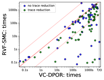
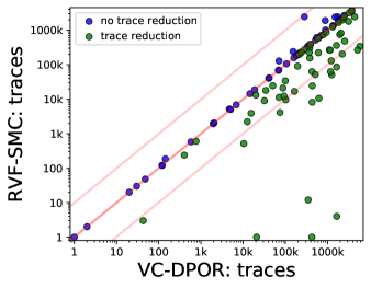
Figure 7: Runtime and traces comparison of $\operatorname{RVF-SMC}$ with $\operatorname{VC-DPOR}$.

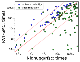
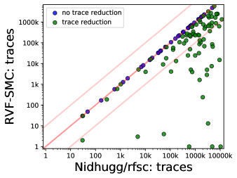
Figure 8: Runtime and traces comparison of $\operatorname{RVF-SMC}$ with $\mathsf{Nidhugg/rfsc}$.

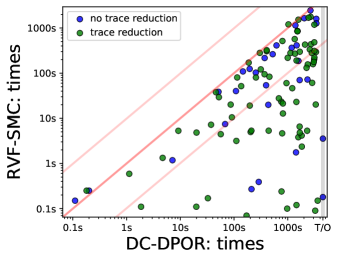
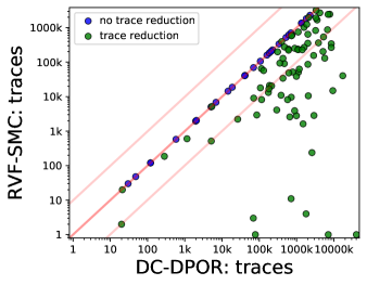
Figure 9: Runtime and traces comparison of $\operatorname{RVF-SMC}$ with $\operatorname{DC-DPOR}$.

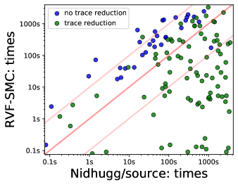
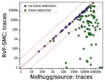
Figure 10: Runtime and traces comparison of $\operatorname{RVF-SMC}$ with $\mathsf{Nidhugg/source}$.

Results. We provide a number of scatter plots summarizing the comparison of $\operatorname{RVF-SMC}$ with other state-of-the-art tools. In Figure 7, Figure 8, Figure 9 and Figure 10 we provide comparison both in runtimes and explored traces, for $\operatorname{VC-DPOR}$, $\mathsf{Nidhugg/rfsc}$, $\operatorname{DC-DPOR}$, and $\mathsf{Nidhugg/source}$, respectively. In each scatter plot, both its axes are log-scaled, the opaque red line represents equality, and the two semi-transparent lines represent an order-of-magnitude difference. The points are colored green when $\operatorname{RVF-SMC}$ achieves trace reduction in the underlying benchmark, and blue otherwise.

Discussion: Significant trace reduction. In Table 1 we provide the results for several benchmarks where $\mathsf{RVF}$ achieves significant reduction in the trace-partitioning size. This is typically accompanied by significant runtime reduction, allowing is to scale the benchmarks to unroll bounds that other tools cannot handle. Examples of this are 27_Boop4 and scull_loop, two toy Linux kernel drivers.

In several benchmarks the number of explored traces remains the same for $\operatorname{RVF-SMC}$ even when scaling up the unroll bound, see 45_monabsex1, reorder_5 and singleton in Table 1. The singleton example is further interesting, in that while $\operatorname{VC-DPOR}$ and $\operatorname{DC-DPOR}$ also explore few traces, they still suffer in runtime due to additional redundant exploration, as described in Sections 1 and 5.

Discussion: Little-to-no trace reduction. Table 2 presents several benchmarks where the $\mathsf{RVF}$ partitioning achieves little-to-no reduction. In these cases the well-engineered $\mathsf{Nidhugg/rfsc}$ and $\mathsf{Nidhugg/source}$ dominate the runtime.

$\operatorname{RVF-SMC}$ ablation studies. Here we demonstrate the effect that follows from our $\operatorname{RVF-SMC}$ algorithm utilizing the approach of backtrack signals (see Section 5) and the heuristics of $\operatorname{VerifySC}$ (see Section 4.2). These techniques have no effect on the number of the explored traces, thus we focus on the runtime. The left plot of Figure 11 compares $\operatorname{RVF-SMC}$ as is with a $\operatorname{RVF-SMC}$ version that does not utilize the backtrack signals (achieved by simply keeping the $\mathsf{backtrack}$ flag in Algorithm 2 always $\mathsf{true}$). The right plot of Figure 11 compares $\operatorname{RVF-SMC}$ as is with a $\operatorname{RVF-SMC}$ version that employs $\operatorname{VerifySC}$ without the closure and auxiliary-trace heuristics. We can see that the techniques almost always result in improved runtime. The improvement is mostly within an order of magnitude, and in a few cases there is several-orders-of-magnitude improvement.

Benchmark		U	$\operatorname{RVF-SMC}$	$\operatorname{VC-DPOR}$	$\mathsf{Nidh/rfsc}$	$\operatorname{DC-DPOR}$	$\mathsf{Nidh/source}$
27_Boop4 threads: 4	Traces	10	1337215	1574287	11610040	-	-
		12	2893039	-	-	-	-
	Times	10	837s	1946s	2616s	-	-
		12	2017s	-	-	-	-
45_monabsex1 threads: U	Traces	7	1	423360	262144	7073803	25401600
		8	1	-	4782969	-	-
	Times	7	0.09s	784s	33s	3239s	2819s
		8	0.09s	-	677s	-	-
reorder_5 threads: U+1	Traces	9	4	1644716	1540	1792290	-
		30	4	-	54901	-	-
	Times	9	0.10s	1711s	0.44s	974s	-
		30	0.09s	-	49s	-	-
scull_loop threads: 3	Traces	2	3908	15394	749811	884443	3157281
		3	115032	-	-	-	-
	Times	2	6.55s	83s	403s	1659s	1116s
		3	266s	-	-	-	-
singleton threads: U+1	Traces	20	2	2	20	20	-
		30	2	-	30	-	-
	Times	20	0.07s	179s	0.08s	171s	-
		30	0.08s	-	0.10s	-	-

Table 1: Benchmarks with trace reduction achieved by $\operatorname{RVF-SMC}$. The unroll bound is shown in the column U. Symbol “-” indicates one-hour timeout. Bold-font entries indicate the smallest numbers for respective benchmark and unroll.

Benchmark		U	$\operatorname{RVF-SMC}$	$\operatorname{VC-DPOR}$	$\mathsf{Nidh/rfsc}$	$\operatorname{DC-DPOR}$	$\mathsf{Nidh/source}$
13_unverif threads: U	Traces	5	14400	14400	14400	14400	14400
		6	518400	-	518400	-	518400
	Times	5	7.45s	63s	3.33s	68s	2.72s
		6	376s	-	134s	-	84s
approxds_append threads: U	Traces	6	50897	1256381	198936	1114746	9847080
		7	923526	-	4645207	-	-
	Times	6	60s	995s	67s	944s	2733s
		7	2078s	-	2003s	-	-
chase-lev-dq threads: 3	Traces	4	87807	$\dagger$	175331	$\dagger$	175331
		5	227654	$\dagger$	448905	$\dagger$	448905
	Times	4	289s	$\dagger$	71s	$\dagger$	71s
		5	995s	$\dagger$	210s	$\dagger$	200s
linuxrwlocks threads: U+1	Traces	1	56	$\dagger$	59	$\dagger$	59
		2	62018	$\dagger$	70026	$\dagger$	70026
	Times	1	0.12s	$\dagger$	0.09s	$\dagger$	0.13s
		2	42s	$\dagger$	15s	$\dagger$	9.50s
pgsql threads: 2	Traces	3	3906	3906	3906	3906	3906
		4	335923	335923	335923	335923	335923
	Times	3	3.30s	5.98s	1.01s	4.00s	0.51s
		4	412s	911s	107s	616s	51s

Table 2: Benchmarks with little-to-no trace reduction by $\operatorname{RVF-SMC}$. Symbol $\dagger$ indicates that a particular benchmark operation is not handled by the tool.

Finally, in Figure 12 we illustrate how much time during $\operatorname{RVF-SMC}$ is typically spent on $\operatorname{VerifySC}$ (i.e., on solving $\operatorname{VSC}$ instances generated during $\operatorname{RVF-SMC}$).

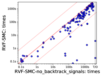
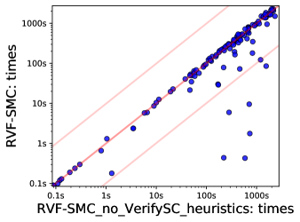
Figure 11: Ablation studies of $\operatorname{RVF-SMC}$. The left plot compares $\operatorname{RVF-SMC}$ with and without backtrack signals. The right plots compares $\operatorname{RVF-SMC}$ with and without the closure and auxiliary-trace heuristics of Section 4.2.

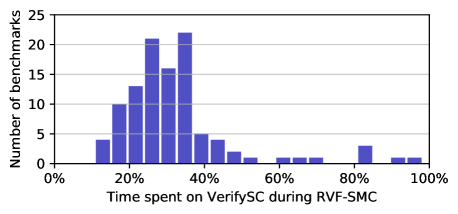
Figure 12: Histogram that illustrates the percentage of time spent solving $\operatorname{VSC}$ instances during $\operatorname{RVF-SMC}$.

7 Conclusions

In this work we developed $\operatorname{RVF-SMC}$, a new SMC algorithm for the verification of concurrent programs using a novel equivalence called reads-value-from (RVF). On our way to $\operatorname{RVF-SMC}$, we have revisited the famous $\operatorname{VSC}$ problem [25]. Despite its NP-hardness, we have shown that the problem is parameterizable in $k+d$ (for $k$ threads and $d$ variables), and becomes even fixed-parameter tractable in $d$ when $k$ is constant. Moreover we have developed practical heuristics that solve the problem efficiently in many practical settings.

Our $\operatorname{RVF-SMC}$ algorithm couples our solution for $\operatorname{VSC}$ to a novel exploration of the underlying RVF partitioning, and is able to model check many concurrent programs where previous approaches time-out. Our experimental evaluation reveals that RVF is very often the most effective equivalence, as the underlying partitioning is exponentially coarser than other approaches. Moreover, $\operatorname{RVF-SMC}$ generates representatives very efficiently, as the reduction in the partitioning is often met with significant speed-ups in the model checking task. Interesting future work includes further improvements over the $\operatorname{VSC}$, as well as extensions of $\operatorname{RVF-SMC}$ to relaxed memory models.

Acknowledgments. The research was partially funded by the ERC CoG 863818 (ForM-SMArt) and the Vienna Science and Technology Fund (WWTF) through project ICT15-003.

Appendix 0.A Extensions of the concurrent model

For presentation clarity, in our exposition we considered a simple concurrent model with a static set of threads, and with only read and write events. Here we describe how our approach handles the following extensions of the concurrent model:

1. Read-modify-write and compare-and-swap events.

2. Mutex events lock-acquire and lock-release.

3. Spawn and join events for dynamic thread creation.

Read-modify-write and compare-and-swap events. We model a read-modify-write atomic operation on a variable $x$ as a pair of two events $\mathit{rmw}_{r}$ and $\mathit{rmw}_{w}$, where $\mathit{rmw}_{r}$ is a read event of $x$, $\mathit{rmw}_{w}$ is a write event of $x$, and for each trace $\sigma$ either the events are both not present in $\sigma$, or they are both present and appearing together in $\sigma$ ($\mathit{rmw}_{r}$ immediately followed by $\mathit{rmw}_{w}$ in $\sigma$). We model a compare-and-swap atomic operation similarly, obtaining a pair of events $\mathit{cas}_{r}$ and $\mathit{cas}_{w}$. In addition we consider a local event happening immediately after the read event $\mathit{cas}_{r}$, evaluating the “compare” condition of the compare-and-swap instruction. Thus, in traces $\sigma$ that contain $\mathit{cas}_{r}$ and the “compare” condition evaluates to $\mathsf{true}$, we have that $\mathit{cas}_{r}$ is immediately followed by $\mathit{cas}_{w}$ in $\sigma$. In traces $\sigma^{\prime}$ that contain $\mathit{cas}_{r}$ and the “compare” condition evaluates to $\mathsf{false}$, we have that $\mathit{cas}_{w}$ is not present in $\sigma^{\prime}$.

We now discuss our extension of $\operatorname{VerifySC}$ to handle the $\operatorname{VSC}(X,\mathsf{GoodW})$ problem (Section 4) in presence of read-modify-write and compare-and-swap events. First, observe that as the event set $X$ and the good-writes function $\mathsf{GoodW}$ are fixed, we possess the information on whether each compare-and-swap instruction satisfies its “compare” condition or not. Then, in case we have in our event set a read-modify-write event pair $e_{1}=\mathit{rmw}_{r}$ and $e_{2}=\mathit{rmw}_{w}$ (resp. a compare-and-swap event pair $e_{1}=\mathit{cas}_{r}$ and $e_{2}=\mathit{cas}_{w}$), we proceed as follows. When the first of the two events $e_{1}$ becomes executable in Algorithm 1 of Algorithm 1 for $\tau$, we proceed only in case $e_{2}$ is also executable in $\tau\circ e_{1}$, and in such a case in Algorithm 1 we consider straight away a sequence $\tau\circ e_{1}\circ e_{2}$. This ensures that in all sequences we consider, the event pair of the read-modify-write (resp. compare-and-swap) appears as one event immediately followed by the other event.

In the presence of read-modify-write and compare-and-swap events, the SMC approach $\operatorname{RVF-SMC}$ can be utilized as presented in Section 5, after an additional corner case is handled for backtrack signals. Specifically, when processing the extension events in Algorithm 2 of Algorithm 2, we additionally process in the same fashion reads $\mathit{cas}_{r}$ enabled in $\widetilde{\sigma}$ that are part of a compare-and-swap instruction. These reads $\mathit{cas}_{r}$ are then treated as potential novel reads-from sources for ancestor mutations $\mathit{cas}^{*}_{r}\in\mathsf{dom}(\mathsf{ancestors})$ (Algorithm 2) where $\mathit{cas}^{*}_{r}$ is also a read-part of a compare-and-swap instruction.

Mutex events. Mutex events $\mathsf{acquire}$ and $\mathsf{release}$ are naturally handled by our approach as follows. We consider each lock-release event $\mathsf{release}$ as a write event and each lock-acquire event $\mathsf{acquire}$ as a read event, the corresponding unique mutex they access is considered a global variable of $\mathcal{G}$.

In SMC, we enumerate good-writes functions whose domain also includes the lock-acquire events. Further, a good-writes set of each lock-acquire admits only a single conflicting lock-release event, thus obtaining constraints of the form $\mathsf{GoodW}(\mathsf{acquire})=\{\mathsf{release}\}$. During closure (Section 4.2), given $\mathsf{GoodW}(\mathsf{acquire})=\{\mathsf{release}\}$, we consider the following condition: $\mathsf{thr}(\mathsf{acquire})\neq\mathsf{thr}(\mathsf{release})$ implies $\mathsf{release}<_{P}\mathsf{acquire}$. Thus $P$ totally orders the critical sections of each mutex, and therefore $\operatorname{VerifySC}$ does not need to take additional care for mutexes. Indeed, respecting $P$ trivially solves all $\mathsf{GoodW}$ constraints of lock-acquire events, and further preserves the property that no thread tries to acquire an already acquired (and so-far unreleased) mutex. No modifications to the $\operatorname{RVF-SMC}$ algorithm are needed to incorporate mutex events.

Dynamic thread creation. For simplicity of presentation, we assumed a static set of threads for a given concurrent program. However, our approach straightforwardly handles dynamic thread creating, by including in the program order $\mathsf{PO}$ the orderings naturally induced by spawn and join events. In our experiments, all our considered benchmarks spawn threads dynamically.

Appendix 0.B Details of Section 3

Consider the simple programs of Figure 13. In each program, all traces of the program are pairwise $\mathsf{RVF}$-equivalent, while the other equivalences induce exponentially many inequivalent traces.

$$\;\text{Thread}_{1}$$

$$w(x,1)$$

$$w(x,1)$$

$$...$$

$$w(x,1)$$

$$w(x,1)$$

$$\text{Thread}_{2}$$

$$w(x,1)$$

$$r(x)$$

$$...$$

$$w(x,1)$$

$$r(x)$$

$$\;\text{Thread}_{3}$$

$$w(x,1)$$

$$w(x,1)$$

$$...$$

$$w(x,1)$$

$$w(x,1)$$

(a) Many operations on one variable.

$$\;\text{Thread}_{1}$$

$$w(x_{1},1)$$

$$w(x_{2},1)$$

$$...$$

$$w(x_{n-1},1)$$

$$w(x_{n},1)$$

$$\text{Thread}_{2}$$

$$w(x_{1},1)$$

$$r(x_{1})$$

$$...$$

$$w(x_{n},1)$$

$$r(x_{n})$$

$$\;\text{Thread}_{3}$$

$$w(x_{1},1)$$

$$w(x_{2},1)$$

$$...$$

$$w(x_{n-1},1)$$

$$w(x_{n},1)$$

(b) Few operations on many variables.

$$\text{Thread}_{1}$$

$$w(x,1)$$

$$r(x)$$

…..

$$\text{Thread}_{n}$$

$$w(x,1)$$

$$r(x)$$

(c) Many threads and one variable.

Figure 13: Programs with one $\mathsf{RVF}$-equivalence class, and $\Omega(2^{n})$ equivalence classes for the reads-from, value-centric, data-centric, and Mazurkiewicz equivalence.

Appendix 0.C Details of Section 4

Here we present the proof of Theorem 4.1.

See 4.1

Proof

We argue separately about soundness, completeness, and complexity of $\operatorname{VerifySC}$ (Algorithm 1).

Soundness. We prove by induction that each sequence in the worklist $\mathcal{S}$ is a witness prefix. The base case with an empty sequence trivially holds. For an inductive case, observe that extending a witness prefix $\tau$ with an event $e$ executable in $\tau$ yields a witness prefix. Indeed, if $e$ is a read, it has an active good-write in $\tau$, thus its good-writes condition is satisfied in $\tau\circ e$. If $e$ is a write, new reads $r$ may start holding the variable $\mathsf{var}(e)$ in $\tau\circ e$, but for all these reads $e$ is its good-write, and it shall be active in $\tau\circ e$. Hence the soundness follows.

Completeness. First notice that for each witness $\tau$ of $\operatorname{VSC}(X,\mathsf{GoodW})$, each prefix of $\tau$ is a witness prefix. What remains to prove is that given two witness prefixes $\tau_{1}$ and $\tau_{2}$ with equal induced witness state, if a suffix exists to extend $\tau_{1}$ to a witness of $\operatorname{VSC}(X,\mathsf{GoodW})$, then such suffix also exists for $\tau_{2}$. Note that since $\tau_{1}$ and $\tau_{2}$ have an equal witness state, their length equals too (since $\mathcal{E}(\tau_{1})=\mathcal{E}(\tau_{2})$). We thus prove the argument by induction with respect to $|X\setminus\mathcal{E}(\tau_{1})|$, i.e., the number of events remaining to add to $\tau_{1}$ resp. $\tau_{2}$. The base case with $|X\setminus\mathcal{E}(\tau_{1})|=0$ is trivially satisfied. For the inductive case, let there be an arbitrary suffix $\tau^{*}$ such that $\tau_{1}\circ\tau^{*}$ is a witness of $\operatorname{VSC}(X,\mathsf{GoodW})$. Let $e$ be the first event of $\tau^{*}$, we have that $\tau_{1}\circ e$ is a witness prefix. Note that $\tau_{2}\circ e$ is also a witness prefix. Indeed, if $e$ is a read, the equality of the memory maps $\operatorname{MMap}_{\tau_{1}}$ and $\operatorname{MMap}_{\tau_{2}}$ implies that since $e$ reads a good-write in $\tau_{1}\circ e$, it also reads the same good-write in $\tau_{2}\circ e$. If $e$ is a write, since $\mathcal{E}(\tau_{1})=\mathcal{E}(\tau_{2})$, each read either holds its variable in both $\tau_{1}$ and $\tau_{2}$ or it does not hold its variable in either of $\tau_{1}$ and $\tau_{2}$. Finally observe that $\operatorname{MMap}_{\tau_{1}\circ e}=\operatorname{MMap}_{\tau_{2}\circ e}$. We have $\operatorname{MMap}_{\tau_{1}}=\operatorname{MMap}_{\tau_{2}}$, if $e$ is a read both memory maps do not change, and if $e$ is a write the only change of the memory maps as compared to $\operatorname{MMap}_{\tau_{1}}$ and $\operatorname{MMap}_{\tau_{2}}$ is that $\operatorname{MMap}_{\tau_{1}\circ e}(\mathsf{var}(e))=\operatorname{MMap}_{\tau_{2}\circ e}(\mathsf{var}(e))=\mathsf{thr}(e)$. Hence we have that $\tau_{1}\circ e$ and $\tau_{2}\circ e$ are both witness prefixes with the same induced witness state, and we can apply our induction hypothesis.

Complexity. There are at most $n^{k}\cdot k^{d}$ pairwise distinct witness states, since the number of different lower sets of $(X,\mathsf{PO})$ is bounded by $n^{k}$, and the number of different memory maps is bounded by $k^{d}$. Hence we have a bound $n^{k}\cdot k^{d}$ on the number of iterations of the main while-loop in Algorithm 1. Further, each iteration of the main while-loop spends $O(n\cdot k)$ time. Indeed, there are at most $k$ iterations of the for-loop in Algorithm 1, in each iteration it takes $O(n)$ time to check whether the event is executable, and the other items take constant time (manipulating $\mathsf{Done}$ in Algorithm 1 and Algorithm 1 takes amortized constant time with hash sets).

∎

Appendix 0.D Details of Section 5

In this section we present the proofs of Lemma 1 and Theorem 5.1. We first prove Lemma 1, and then we refer to it when proving Theorem 5.1.

See 1

Proof

We prove the statement by a sequence of reasoning steps.

1. Let $S$ be the set of writes $w^{*}\not\in\mathcal{W}(\widetilde{\sigma})$ such that there exists a trace $\sigma^{*}$ that (i) satisfies $\mathsf{GoodW}$ and $\mathcal{C}$, and (ii) contains $r$ with $\mathsf{RF}_{\sigma^{*}}(r)=w^{*}$. Observe that $\mathsf{RF}_{\sigma^{\prime}}(r)\in S$, hence $S$ is nonempty.

2. Let $Y$ be the set of events containing $r$ and the causal future of $r$ in $\sigma^{\prime}$, formally $Y=\{e\in\mathcal{E}(\sigma^{\prime})\;|\;r\mathsf{\mapsto}_{\sigma}e\}\cup\{r\}$. Observe that $Y\cap\mathcal{E}(\widetilde{\sigma})=\emptyset$. Consider a subsequence $\sigma^{\prime\prime}=\sigma^{\prime}|(\mathcal{E}(\sigma^{\prime})\setminus Y)$ (i.e., subsequence of all events except $Y$). $\sigma^{\prime\prime}$ is a valid trace, and from $Y\cap\mathcal{E}(\widetilde{\sigma})=\emptyset$ we get that $\sigma^{\prime\prime}$ satisfies $\mathsf{GoodW}$ and $\mathcal{C}$.

3. Let $T_{1}$ be the set of all partial traces that (i) contain all of $\mathcal{E}(\widetilde{\sigma})$, (ii) satisfy $\mathsf{GoodW}$ and $\mathcal{C}$, (iii) do not contain r, and (iv) contain some $w^{*}\in S$. $T_{1}$ is nonempty due to (2).

4. Let $T_{2}\subseteq T_{1}$ be the traces $\sigma^{*}$ of $T_{1}$ where for each $w^{*}\in S\cap\mathcal{E}(\sigma^{*})$, we have that $w^{*}$ is the last event of its thread in $\sigma^{*}$. The set $T_{2}$ is nonempty: since $w^{*}\not\in\mathcal{W}(\widetilde{\sigma})$, the events of its causal future in $\sigma^{*}$ are also not in $\mathcal{E}(\widetilde{\sigma})$, and thus they are not good-writes to any read in $\mathsf{GoodW}$.

5. Let $T_{3}\subseteq T_{2}$ be the traces of $T_{2}$ with the least amount of read events in total. Trivially $T_{3}$ is nonempty. Further note that in each trace $\sigma^{*}\in T_{3}$, no read reads-from any write $w^{*}\in S\cap\mathcal{E}(\sigma^{*})$. Indeed, such write can only be read-from by reads $r^{*}$ out of $\mathcal{E}(\widetilde{\sigma})$ (traces of $T_{3}$ satisfy $\mathsf{GoodW}$). Further, events of the causal future of such reads $r^{*}$ are not good-writes to any read in $\mathsf{GoodW}$ (they are all out of $\mathcal{E}(\widetilde{\sigma})$). Thus the presence of $r^{*}$ violates the property of having the least amount of read events in total.

6. Let $\sigma_{1}$ be an arbitrary partial trace from $T_{3}$. Let $S_{1}=S\cap\mathcal{E}(\sigma_{1})$, by (3) we have that $S_{1}$ is nonempty. Let $\sigma_{2}=\sigma_{1}|(\mathcal{E}(\sigma_{1})\setminus S_{1})$. Note that $\sigma_{2}$ is a valid trace, as for each $w^{*}\in S_{1}$, by (4) it is the last event of its thread, and by (5) it is not read-from by any read in $\sigma_{1}$.

7. Since $r\in\mathsf{enabled}(\widetilde{\sigma})$ and $\mathcal{E}(\widetilde{\sigma})\subseteq\mathcal{E}(\sigma_{2})$ and $r\not\in\mathcal{E}(\sigma_{2})$, we have that $r\in\mathsf{enabled}(\sigma_{2})$. Let $w^{*}\in S_{1}$ arbitrary, by the previous step we have $w^{*}\in\mathsf{enabled}(\sigma_{2})$. Now consider $\mkern 1.5mu\overline{\mkern-1.5mu\sigma\mkern-1.5mu}\mkern 1.5mu=\sigma_{2}\circ r\circ w^{*}$. Notice that (i) $\mkern 1.5mu\overline{\mkern-1.5mu\sigma\mkern-1.5mu}\mkern 1.5mu$ satisfies $\mathsf{GoodW}$ and $\mathcal{C}$, (ii) $\mathsf{RF}_{\mkern 1.5mu\overline{\mkern-1.5mu\sigma\mkern-1.5mu}\mkern 1.5mu}(r)\in\mathcal{W}(\widetilde{\sigma})$ (there is no write out of $\mathcal{W}(\widetilde{\sigma})$ present in $\sigma_{2}$), and (iii) for $w^{*}\in\mathcal{E}(\mkern 1.5mu\overline{\mkern-1.5mu\sigma\mkern-1.5mu}\mkern 1.5mu)$, since $w^{*}\in S$ we have $r\Join w^{*}$ and $\mathsf{thr}(r)\neq\mathsf{thr}(w^{*})$.

∎

Now we are ready to prove Theorem 5.1.

See 5.1

Proof

We argue separately about soundness, completeness, and complexity.

Soundness. The soundness of $\operatorname{RVF-SMC}$ follows from the soundness of $\operatorname{VerifySC}$ used as a subroutine to generate traces that $\operatorname{RVF-SMC}$ considers.

Completeness. Let $nd=\operatorname{RVF-SMC}(X,\mathsf{GoodW},\sigma,\mathcal{C})$ be an arbitrary recursion node of $\operatorname{RVF-SMC}$. Let $\sigma^{\prime}$ be an arbitrary valid full program trace satisfying $\mathsf{GoodW}$ and $\mathcal{C}$. The goal is to prove that the exploration rooted at $a$ explores a good-writes function $\mathsf{GoodW}^{\prime}\colon\mathcal{R}(\sigma^{\prime})\to 2^{\mathcal{W}(\sigma^{\prime})}$ such that for each $r\in\mathcal{R}(\sigma^{\prime})$ we have $\mathsf{RF}_{\sigma^{\prime}}(r)\in\mathsf{GoodW}^{\prime}(r)$.

We prove the statement by induction in the length of maximal possible extension, i.e., the largest possible number of reads not defined in $\mathsf{GoodW}$ that a valid full program trace satisfying $\mathsf{GoodW}$ and $\mathcal{C}$ can have. As a reminder, given $nd=\operatorname{RVF-SMC}(X,\mathsf{GoodW},\sigma,\mathcal{C})$ we first consider a trace $\widetilde{\sigma}=\sigma\circ\widehat{\sigma}$ where $\widehat{\sigma}$ is a maximal extension such that no event of $\widehat{\sigma}$ is a read.

Base case: 1. There is exactly one enabled read $r\in\mathsf{enabled}(\widetilde{\sigma})$. All other threads have no enabled event, i.e., they are fully extended in $\widetilde{\sigma}$. Because of this, our algorithm considers every possible source $r$ can read-from in traces satisfying $\mathsf{GoodW}$ and $\mathcal{C}$. Completeness of $\operatorname{VerifySC}$ then implies completeness of this base case.

Inductive case. Let ${\sf MAXEXT}$ be the length of maximal possible extension of $nd=\operatorname{RVF-SMC}(X,\mathsf{GoodW},\sigma,\mathcal{C})$. By induction hypothesis, $\operatorname{RVF-SMC}$ is complete when rooted at any node with maximal possible extension length ${\sf<MAXEXT}$. The rest of the proof is to prove completeness when rooted at $nd$, and the desired result then follows.

Inductive case: $\operatorname{RVF-SMC}$ without backtrack signals. We first consider a simpler version of $\operatorname{RVF-SMC}$, where the boolean signal $\mathsf{backtrack}$ is always set to $\mathsf{true}$ (i.e., Algorithm 2 without Algorithm 2). After we prove the inductive case of this version, we use it to prove the inductive case of the full version of $\operatorname{RVF-SMC}$.

Let $r_{1},...,r_{k}$ be the enabled events in $\widetilde{\sigma}$, $nd$ proceeds with recursive calls in that order (i.e., first with $r_{1}$, then with $r_{2}$, …, last with $r_{k}$). Let $\sigma^{\prime}$ be an arbitrary valid full program trace satisfying $\mathsf{GoodW}$ and $\mathcal{C}$. Trivially, $\sigma^{\prime}$ contains all of $r_{1},...,r_{k}$. Consider their reads-from sources $\mathsf{RF}_{\sigma^{\prime}}(r_{1}),...,\mathsf{RF}_{\sigma^{\prime}}(r_{k})$. Now consider two cases:

1. There exists $1\leq i\leq k$ such that $\mathsf{RF}_{\sigma^{\prime}}(r_{i})\in\mathcal{E}(\widetilde{\sigma})\cup\{\mathsf{init\_event}\}$.

2. There exists no such $i$.

Let us prove that (2) is impossible. By contradiction, consider it possible, let $r_{j}$ be the first read out of $r_{1},...,r_{k}$ in the order as appearing in $\sigma^{\prime}$. Consider the thread of $\mathsf{RF}_{\sigma^{\prime}}(r_{j})$. It has to be one of $\mathsf{thr}{r_{1}},...,\mathsf{thr}{r_{k}}$, as other threads have no enabled event in $\widetilde{\sigma}$, thus they are fully extended in $\widetilde{\sigma}$. It cannot be $\mathsf{thr}{r_{j}}$, because all thread-predecessors of $r_{j}$ are in $\mathcal{E}(\widetilde{\sigma})$. Thus let it be a thread $1\leq m\leq k,m\neq j$. Since $\mathsf{RF}_{\sigma^{\prime}}(r_{j})\not\in\mathcal{E}(\widetilde{\sigma})$, $\mathsf{RF}_{\sigma^{\prime}}(r_{j})$ comes after $r_{m}$ in $\sigma^{\prime}$. This gives us $r_{m}<_{\sigma^{\prime}}\mathsf{RF}_{\sigma^{\prime}}(r_{j})<_{\sigma^{\prime}}r_{j}$, which is a contradiction with $r_{j}$ being the first out of $r_{1},...,r_{k}$ in $\sigma^{\prime}$. Hence we know that above case (1) is the only possibility.

Let $1\leq j\leq k$ be the smallest with $\mathsf{RF}_{\sigma^{\prime}}(r_{j})\in\mathcal{E}(\widetilde{\sigma})\cup\{\mathsf{init\_event}\}$. Since $\sigma^{\prime}$ satisfies $\mathsf{GoodW}$ and $\mathcal{C}$, we have $\mathsf{RF}_{\sigma^{\prime}}(r_{j})\not\in\mathcal{C}(r_{j})$. Consider $nd$ performing a recursive call with $r_{j}$. Since $\mathsf{RF}_{\sigma^{\prime}}(r_{j})\in\mathcal{E}(\widetilde{\sigma})\cup\{\mathsf{init\_event}\}$ and $\mathsf{RF}_{\sigma^{\prime}}(r_{j})\not\in\mathcal{C}(r_{j})$, $nd$ considers for $r_{j}$ (among others) a good-writes set $\mathsf{GoodW}_{j}$ that contains $\mathsf{RF}_{\sigma^{\prime}}(r_{j})$, and by completeness of $\operatorname{VSC}$, we correctly classify $\mathsf{GoodW}\cup\{(r_{j},\mathsf{GoodW}_{j})\}$ as realizable. This creates a recursive call with the following $\mkern 1.5mu\overline{\mkern-1.5mund\mkern-1.5mu}\mkern 1.5mu=\operatorname{RVF-SMC}(\mkern 1.5mu\overline{\mkern-1.5muX\mkern-1.5mu}\mkern 1.5mu,\mkern 1.5mu\overline{\mkern-1.5mu\mathsf{GoodW}\mkern-1.5mu}\mkern 1.5mu,\mkern 1.5mu\overline{\mkern-1.5mu\sigma\mkern-1.5mu}\mkern 1.5mu,\mkern 1.5mu\overline{\mkern-1.5mu\mathcal{C})\mkern-1.5mu}\mkern 1.5mu$:

1. $\mkern 1.5mu\overline{\mkern-1.5muX\mkern-1.5mu}\mkern 1.5mu=\mathcal{E}(\widetilde{\sigma})\cup\{r_{j}\}$.

2. $\mkern 1.5mu\overline{\mkern-1.5mu\mathsf{GoodW}\mkern-1.5mu}\mkern 1.5mu=\mathsf{GoodW}\cup\{(r_{j},\mathsf{GoodW}_{j})\}$.

3. $\mkern 1.5mu\overline{\mkern-1.5mu\sigma\mkern-1.5mu}\mkern 1.5mu$ is a witness trace, i.e., valid program trace satisfying $\mkern 1.5mu\overline{\mkern-1.5mu\mathsf{GoodW}\mkern-1.5mu}\mkern 1.5mu$.

4. $\mkern 1.5mu\overline{\mkern-1.5mu\mathcal{C})\mkern-1.5mu}\mkern 1.5mu=\mathcal{C}\cup\{(r_{i},\mathcal{C}_{i})\;|\>1\leq i<j\}$ where $\mathcal{C}_{i}$ are the writes of $\mathsf{var}(r_{i})$ in $\mathcal{E}(\widetilde{\sigma})\cup\{\mathsf{init\_event}\}$.

Clearly $\sigma^{\prime}$ satisfies $\mkern 1.5mu\overline{\mkern-1.5mu\mathsf{GoodW}\mkern-1.5mu}\mkern 1.5mu$. Note that $\sigma^{\prime}$ also satisfies $\mkern 1.5mu\overline{\mkern-1.5mu\mathcal{C})\mkern-1.5mu}\mkern 1.5mu$, as it satisfies $\mathcal{C}$, and for each $1\leq i<j$, we have $\mathsf{RF}_{\sigma^{\prime}}(r_{i})\not\in\mathcal{C}_{i}$, as $\mathsf{RF}_{\sigma^{\prime}}(r_{i})\not\in\mathcal{E}(\widetilde{\sigma})\cup\{\mathsf{init\_event}\}$. Hence we can apply our inductive hypothesis for $\mkern 1.5mu\overline{\mkern-1.5mund\mkern-1.5mu}\mkern 1.5mu$, and we’re done.

Inductive case: $\operatorname{RVF-SMC}$. Let $r_{1},...,r_{m}$ be the enabled events (reads) in $\widetilde{\sigma}$ not defined in $\mathcal{C}$, and let $r_{m+1},...,r_{k}$ be the enabled events defined in $\mathcal{C}$. The node $nd$ proceeds with the recursive calls as follows:

1. $nd$ processes calls with $r_{1}$, stops if $\mathsf{backtrack}=\mathsf{false}$ (Algorithm 2), else:

2. $nd$ processes calls with $r_{2}$, stops if $\mathsf{backtrack}=\mathsf{false}$, else …..

3. $nd$ processes calls with $r_{m}$, stops if $\mathsf{backtrack}=\mathsf{false}$, else

4. $nd$ processes calls with $r_{m}$, then $r_{m+1}$, …, finally $r_{k}$.

Let $\sigma^{\prime}$ be an arbitrary valid full program trace satisfying $\mathsf{GoodW}$ and $\mathcal{C}$. Trivially, $\sigma^{\prime}$ contains all of $r_{1},...,r_{k}$. Consider their reads-from sources $\mathsf{RF}_{\sigma^{\prime}}(r_{1}),...,\mathsf{RF}_{\sigma^{\prime}}(r_{k})$. Let $1\leq j\leq k$ be the smallest with $\mathsf{RF}_{\sigma^{\prime}}(r_{j})\in\mathcal{E}(\widetilde{\sigma})\cup\{\mathsf{init\_event}\}$. From the above paragraph, we have that such $j$ exists. From the above paragraph we also have that $nd$ processing calls with $r_{j}$ explores a good-writes function $\mathsf{GoodW}^{\prime}\colon\mathcal{R}(\sigma^{\prime})\to 2^{\mathcal{W}(\sigma^{\prime})}$ such that for each $r\in\mathcal{R}(\sigma^{\prime})$ we have $\mathsf{RF}_{\sigma^{\prime}}(r)\in\mathsf{GoodW}^{\prime}(r)$. What remains to prove is that $nd$ will reach the point of processing calls with $r_{j}$. That amounts to proving that for each $1\leq x\leq\min(m,j-1)$, $nd$ receives $\mathsf{backtrack}=\mathsf{true}$ when processing calls with $r_{x}$. For each such $x$, $\mathsf{RF}_{\sigma^{\prime}}(r_{x})\not\in\mathcal{E}(\widetilde{\sigma})\cup\{\mathsf{init\_event}\}$. We construct a trace that matches the antecedent of Lemma 1.

First denote $\sigma^{\prime}=\sigma_{1}\circ\mathsf{RF}_{\sigma^{\prime}}(r_{x})\circ\sigma_{2}$. Let $\sigma_{3}$ be the subsequence of $\sigma_{2}$, containing only events of $\mathcal{E}(\widetilde{\sigma})\cap\mathcal{E}(\sigma_{2})$. Now consider $\sigma_{4}=\sigma_{1}\circ\sigma_{3}\circ\mathsf{RF}_{\sigma^{\prime}}(r_{x})\circ r_{x}$. Note that $\sigma_{4}$ is a valid trace because:

1. Each event of $\mathcal{E}(\sigma_{2})\setminus\mathcal{E}(\widetilde{\sigma})$ appears in its thread only after all events of that thread in $\mathcal{E}(\widetilde{\sigma})$.

2. Each read of $\sigma_{3}$ has $\mathsf{GoodW}$ defined, and $\sigma_{3}$ does not contain $\mathsf{RF}_{\sigma^{\prime}}(r_{x})$ nor any events of $\mathcal{E}(\sigma_{2})\setminus\mathcal{E}(\widetilde{\sigma})$.

3. $\mathsf{RF}_{\sigma^{\prime}}(r_{x})$ is enabled in $\sigma_{1}\circ\sigma_{3}$, since it is already enabled in $\sigma_{1}$.

4. $r_{1}$ is not in $\sigma_{1}$ as those events appear before $\mathsf{RF}_{\sigma^{\prime}}(r_{x})$ in $\sigma^{\prime}$, also $r_{1}$ is not in $\sigma_{3}$ because $r_{1}\not\in\mathcal{E}(\widetilde{\sigma})$. $r_{1}$ is enabled in $\sigma_{1}\circ\sigma_{3}\circ\mathsf{RF}_{\sigma^{\prime}}(r_{x})$ as it contains all events of $\mathcal{E}(\widetilde{\sigma})$.

Hence $\sigma_{4}$ is a valid trace containing all events $\mathcal{E}(\widetilde{\sigma})$. Further $\sigma_{4}$ satisfies $\mathsf{GoodW}$ and $\mathcal{C}$, because $\sigma^{\prime}$ satisfies $\mathsf{GoodW}$ and $\mathcal{C}$ and $\sigma_{4}$ contains the same subsequence of the events $\mathcal{E}(\widetilde{\sigma})$. Finally, $\mathsf{RF}_{\sigma_{4}}(r_{x})=\mathsf{RF}_{\sigma^{\prime}}(r_{x})\not\in\mathcal{W}(\widetilde{\sigma})$. The inductive case, and hence the completeness result, follows.

Complexity. Each recursive call of $\operatorname{RVF-SMC}$ (Algorithm 2) trivially spends $n^{O(k)}$ time in total except the $\operatorname{VerifySC}$ subroutine of Algorithm 2. For the $\operatorname{VerifySC}$ subroutine we utilize the complexity bound $O(n^{k+1}\cdot k^{d+1})$ from Theorem 4.1, thus the total time spent in each call of $\operatorname{RVF-SMC}$ is $n^{O(k)}\cdot O(k^{d})$.

Next we argue that no two leaves of the recursion tree of $\operatorname{RVF-SMC}$ correspond to the same class of the $\mathsf{RVF}$ trace partitioning. For the sake of reaching contradiction, consider two such distinct leaves $l_{1}$ and $l_{2}$. Let $a$ be their last (starting from the root recursion node) common ancestor. Let $c_{1}$ and $c_{2}$ be the child of $a$ on the way to $l_{1}$ and $l_{2}$ respectively. We have $c_{1}\neq c_{2}$ since $a$ is the last common ancestor of $l_{1}$ and $l_{2}$. The recursion proceeds from $a$ to $c_{1}$ (resp. $c_{2}$) by issuing a good-writes set to some read $r_{1}$ (resp. $r_{2}$). If $r_{1}=r_{2}$, then the two good-writes set issued to $r_{1}=r_{2}$ in $a$ differ in the value that the writes of the two sets write (see Algorithm 2 of Algorithm 2). Hence $l_{1}$ and $l_{2}$ cannot represent the same $\mathsf{RVF}$ partitioning class, as representative traces of the two classes shall differ in the value that $r_{1}=r_{2}$ reads. Hence the only remaining possibility is $r_{1}\neq r_{2}$. In iterations of Algorithm 2 in $a$, wlog assume that $r_{1}$ is processed before $r_{2}$. For any pair of traces $\sigma_{1}$ and $\sigma_{2}$ that are class representatives of $l_{1}$ and $l_{2}$ respectively, we have that $\mathsf{RF}_{\sigma_{1}}(r_{1})\neq\mathsf{RF}_{\sigma_{2}}(r_{1})$. This follows from the update of the causal map $\mathcal{C}$ in Algorithm 2 of the Algorithm 2-iteration of $a$ processing $r_{1}$. Further, we have that $\mathsf{RF}_{\sigma_{2}}(r_{1})$ is a thread-successor of a read $\mkern 1.5mu\overline{\mkern-1.5mur\mkern-1.5mu}\mkern 1.5mu\neq r_{1}$ that was among the enabled reads of $\mathsf{mutate}$ in $a$. From this we have $\mkern 1.5mu\overline{\mkern-1.5mur\mkern-1.5mu}\mkern 1.5mu\mathsf{\mapsto}_{\sigma_{2}}r_{1}$ and $\mkern 1.5mu\overline{\mkern-1.5mur\mkern-1.5mu}\mkern 1.5mu\mathsf{\not\mapsto}_{\sigma_{1}}r_{1}$. Thus the traces $\sigma_{1}$ and $\sigma_{2}$ differ in the causal orderings of the read events, contradicting that $l_{1}$ and $l_{2}$ correspond to the same class of the $\mathsf{RVF}$ trace partitioning.

Finally we argue that for each class of the $\mathsf{RVF}$ trace partitioning, represented by the $(X,\mathsf{GoodW})$ of its $\operatorname{RVF-SMC}$ recursion leaf, at most $n^{k}$ calls of $\operatorname{RVF-SMC}$ can be performed where its $X^{\prime}$ and $\mathsf{GoodW}^{\prime}$ are subsets of $X$ and $\mathsf{GoodW}$, respectively. This follows from two observations. First, in each call of $\operatorname{RVF-SMC}$, the event set is extended maximally by enabled writes, and further by one read, while the good-writes function is extended by defining one further read. Second, the amount of lower sets of the partial order $(\mathcal{R}(X),\mathsf{PO})$ is bounded by $n^{k}$.

The desired complexity result follows. ∎

Appendix 0.E Details of Section 6

Here we present additional details on our experimental setup.

Handling assertion violations. Some of the benchmarks in our experiments contain assertion violations, which are successfully detected by all algorithms we consider in our experimental evaluation. After performing this sanity check, we have disabled all assertions, in order to not have the measured parameters be affected by how fast a violation is discovered, as the latter is arbitrary. Our primary experimental goal is to characterize the size of the underlying partitionings, and the time it takes to explore these partitionings.

Identifying events. As mentioned in Section 2, an event is uniquely identified by its predecessors in $\mathsf{PO}$, and by the values its $\mathsf{PO}$-predecessors have read. In our implementation, we rely on the interpreter built inside Nidhugg to identify events. An event $e$ is defined by a pair ($a_{e},b_{e}$), where $a_{e}$ is the thread identifier of $e$ and $b_{e}$ is the sequential number of the last LLVM instruction (of the corresponding thread) that is part of $e$ (the $e$ corresponds to zero or several LLVM instructions not accessing shared variables, and exactly one LLVM instruction accessing a shared variable). It can happen that there exist two traces $\sigma_{1}$ and $\sigma_{2}$, and two different events $e_{1}\in\sigma_{1}$, $e_{2}\in\sigma_{2}$, such that their identifiers are equal, i.e., $a_{e_{1}}=a_{e_{2}}$ and $b_{e_{2}}=b_{e_{2}}$. However, this means that the control-flow leading to each event is different. In this case, $\sigma_{1}$ and $\sigma_{2}$ differ in the value read by a common event that is ordered by the program order $\mathsf{PO}$ both before $e_{1}$ and before $e_{2}$, hence $e_{1}$ and $e_{2}$ are treated as inequivalent.

Technical details. For our experiments we have used a Linux machine with Intel(R) Xeon(R) CPU E5-1650 v3 @ 3.50GHz (12 CPUs) and 128GB of RAM. We have run Nidhugg with Clang and LLVM version 8.

Scatter plots setup. Each scatter plot compares our algorithm $\operatorname{RVF-SMC}$ with some other algorithm $X$. In a fixed plot, each benchmark provides a single data point, obtained as follows. For the benchmark, we consider the highest unroll bound where neither of the algorithms $\operatorname{RVF-SMC}$ and $X$ timed out. Then we plot the times resp. traces obtained on that benchmark and unroll bound by the two algorithms $\operatorname{RVF-SMC}$ and $X$.

References

- [1] Madanlal Musuvathi, Shaz Qadeer, Thomas Ball, Gerard Basler, Piramanayagam Arumuga Nainar, and Iulian Neamtiu. Finding and reproducing heisenbugs in concurrent programs. In OSDI, 2008.
- [2] Edmund M. Clarke, Jr., Orna Grumberg, and Doron A. Peled. Model Checking. MIT Press, Cambridge, MA, USA, 1999.
- [3] Patrice Godefroid. Model checking for programming languages using verisoft. In POPL, 1997.
- [4] Patrice Godefroid. Software model checking: The verisoft approach. FMSD, 26(2):77–101, 2005.
- [5] Tom Ball Madan Musuvathi, Shaz Qadeer. Chess: A systematic testing tool for concurrent software. Technical report, November 2007.
- [6] P. Godefroid. Partial-Order Methods for the Verification of Concurrent Systems: An Approach to the State-Explosion Problem. Springer-Verlag, Secaucus, NJ, USA, 1996.
- [7] Madanlal Musuvathi and Shaz Qadeer. Iterative context bounding for systematic testing of multithreaded programs. SIGPLAN Not., 42(6):446–455, 2007.
- [8] Akash Lal and Thomas Reps. Reducing concurrent analysis under a context bound to sequential analysis. FMSD, 35(1):73–97, 2009.
- [9] Peter Chini, Jonathan Kolberg, Andreas Krebs, Roland Meyer, and Prakash Saivasan. On the Complexity of Bounded Context Switching. In Kirk Pruhs and Christian Sohler, editors, 25th Annual European Symposium on Algorithms (ESA 2017), volume 87 of Leibniz International Proceedings in Informatics (LIPIcs), pages 27:1–27:15, Dagstuhl, Germany, 2017. Schloss Dagstuhl–Leibniz-Zentrum fuer Informatik.
- [10] Pascal Baumann, Rupak Majumdar, Ramanathan S. Thinniyam, and Georg Zetzsche. Context-bounded verification of liveness properties for multithreaded shared-memory programs. Proc. ACM Program. Lang., 5(POPL), January 2021.
- [11] E.M. Clarke, O. Grumberg, M. Minea, and D. Peled. State space reduction using partial order techniques. STTT, 2(3):279–287, 1999.
- [12] Doron Peled. All from one, one for all: On model checking using representatives. In CAV, 1993.
- [13] A Mazurkiewicz. Trace theory. In Advances in Petri Nets 1986, Part II on Petri Nets: Applications and Relationships to Other Models of Concurrency, pages 279–324. Springer-Verlag New York, Inc., 1987.
- [14] Cormac Flanagan and Patrice Godefroid. Dynamic partial-order reduction for model checking software. In POPL, 2005.
- [15] Parosh Abdulla, Stavros Aronis, Bengt Jonsson, and Konstantinos Sagonas. Optimal dynamic partial order reduction. POPL, 2014.
- [16] Huyen T. T. Nguyen, César Rodríguez, Marcelo Sousa, Camille Coti, and Laure Petrucci. Quasi-optimal partial order reduction. In Computer Aided Verification - 30th International Conference, CAV 2018, Held as Part of the Federated Logic Conference, FloC 2018, Oxford, UK, July 14-17, 2018, Proceedings, Part II, pages 354–371, 2018.
- [17] Stavros Aronis, Bengt Jonsson, Magnus Lång, and Konstantinos Sagonas. Optimal dynamic partial order reduction with observers. In Dirk Beyer and Marieke Huisman, editors, Tools and Algorithms for the Construction and Analysis of Systems, pages 229–248, Cham, 2018. Springer International Publishing.
- [18] Patrice Godefroid and Didier Pirottin. Refining dependencies improves partial-order verification methods (extended abstract). In CAV, 1993.
- [19] Elvira Albert, Puri Arenas, María García de la Banda, Miguel Gómez-Zamalloa, and Peter J. Stuckey. Context-sensitive dynamic partial order reduction. In Rupak Majumdar and Viktor Kunčak, editors, Computer Aided Verification, pages 526–543, Cham, 2017. Springer International Publishing.
- [20] Michalis Kokologiannakis, Azalea Raad, and Viktor Vafeiadis. Effective lock handling in stateless model checking. Proc. ACM Program. Lang., 3(OOPSLA), October 2019.
- [21] Marek Chalupa, Krishnendu Chatterjee, Andreas Pavlogiannis, Nishant Sinha, and Kapil Vaidya. Data-centric dynamic partial order reduction. Proc. ACM Program. Lang., 2(POPL):31:1–31:30, December 2017.
- [22] Parosh Aziz Abdulla, Mohamed Faouzi Atig, Bengt Jonsson, Magnus Lång, Tuan Phong Ngo, and Konstantinos Sagonas. Optimal stateless model checking for reads-from equivalence under sequential consistency. Proc. ACM Program. Lang., 3(OOPSLA), October 2019.
- [23] Krishnendu Chatterjee, Andreas Pavlogiannis, and Viktor Toman. Value-centric dynamic partial order reduction. Proc. ACM Program. Lang., 3(OOPSLA), October 2019.
- [24] Jeff Huang. Stateless model checking concurrent programs with maximal causality reduction. In PLDI, 2015.
- [25] Phillip B. Gibbons and Ephraim Korach. Testing shared memories. SIAM J. Comput., 26(4):1208–1244, August 1997.
- [26] Parosh Aziz Abdulla, Mohamed Faouzi Atig, Bengt Jonsson, and Tuan Phong Ngo. Optimal stateless model checking under the release-acquire semantics. Proc. ACM Program. Lang., 2(OOPSLA):135:1–135:29, 2018.
- [27] Parosh Aziz Abdulla, Stavros Aronis, Mohamed Faouzi Atig, Bengt Jonsson, Carl Leonardsson, and Konstantinos Sagonas. Stateless model checking for tso and pso. In TACAS, 2015.
- [28] Michalis Kokologiannakis, Azalea Raad, and Viktor Vafeiadis. Model checking for weakly consistent libraries. In Proceedings of the 40th ACM SIGPLAN Conference on Programming Language Design and Implementation, PLDI 2019, pages 96–110, New York, NY, USA, 2019. ACM.
- [29] Michalis Kokologiannakis, Ori Lahav, Konstantinos Sagonas, and Viktor Vafeiadis. Effective stateless model checking for c/c++ concurrency. Proc. ACM Program. Lang., 2(POPL):17:1–17:32, December 2017.
- [30] Andreas Pavlogiannis. Fast, sound, and effectively complete dynamic race prediction. Proc. ACM Program. Lang., 4(POPL), December 2019.
- [31] Magnus Lång and Konstantinos Sagonas. Parallel graph-based stateless model checking. In Dang Van Hung and Oleg Sokolsky, editors, ATVA, volume 12302 of Lecture Notes in Computer Science, pages 377–393. Springer, 2020.
- [32] Brian Norris and Brian Demsky. A practical approach for model checking C/C++11 code. ACM Trans. Program. Lang. Syst., 38(3):10:1–10:51, 2016.