An irregularly spaced first-order moving average model

Abstract

A novel first-order moving-average model for analyzing time series observed at irregularly spaced intervals is introduced. Two definitions are presented, which are equivalent under Gaussianity. The first one relies on normally distributed data and the specification of second-order moments. The second definition provided is more flexible in the sense that it allows for considering other distributional assumptions. The statistical properties are investigated along with the one-step linear predictors and their mean squared errors. It is established that the process is strictly stationary under normality and weakly stationary in the general case. Maximum likelihood and bootstrap estimation procedures are discussed and the finite-sample behavior of these estimates is assessed through Monte Carlo experiments. In these simulations, both methods perform well in terms of estimation bias and standard errors, even with relatively small sample sizes. Moreover, we show that for non-Gaussian data, for t-Student and Generalized errors distributions, the parameters of the model can be estimated precisely by maximum likelihood. The proposed IMA model is compared to the continuous autoregressive moving average (CARMA) models, exhibiting good performance. Finally, the practical application and usefulness of the proposed model are illustrated with two real-life data examples.

1 Introduction

Time series data observed at irregularly spaced intervals arise often in fields as diverse as astronomy, climatology, economics, finance, medical sciences, geophysics; see for example moore1987experiences,Muñoz et al. (1992), Belcher et al. (1994), kim2008fitting,Hand (2008), Corduas and Piccolo (2008), Harvill et al. (2013), Podgorski (2014), Babu and Mahabal (2016), Eyheramendy et al. (2018), miller2019testing, Edelmann et al. (2019), Caceres et al. (2019), Elorrieta et al. (2019), and Zhang (2020), among others. In particular, in the climatology context, Mudelsee (2014) points out that conventional time series analysis has largely ignored irregularly spaced structures that climate time series must take into account. The statistical analysis of these data poses several difficulties. First, the overwhelming majority of the available time series methods assume regularly observed data, (see, e.g., Brockwell and Davis, 1991; Hamilton, 1994; Box et al., 2016). Second, when this assumption is dropped, several technical problems arise including the issue of formulating appropriate methodologies for carrying out statistical inferences. Third, most of the currently available numerical algorithms for computing estimators and forecasts are based on the regularity of the data collection process.

Irregularly spaced time series may occur in many ways. For example, data can be regularly spaced with missing observations. On the other hand, data can be truly irregularly spaced with no underlying regular sampling interval. Moreover, a time series may exhibit both irregularly spaced measurements and missing values. This may occur, for example in astronomy where the measurement schedule may be irregularly spaced and the scheduled observation cannot be made at the specified date due to cloudiness.

Techniques considering time series in the presence of missing data are useful when data are regularly spaced with missing observations (see, e.g., Parzen, 1963; Dunsmuir, 1983; Reinsel and Wincek, 1987). Nevertheless, these techniques cannot be applied if data are truly irregularly spaced. This case usually has been treated through two approaches. First, the irregularly spaced time series is transformed into regularly spaced through interpolation and consequently conventional techniques are applied. Adorf (1995) provides a summary of such transformations, which are frequently used to analyze astronomical data. However, interpolation methods typically produce bias (for instance, over-smoothing), changing the dynamic of the process. Second, irregularly spaced time series can be treated as discrete realizations of a continuous stochastic process (see, e.g., Robinson, 1977; Parzen, 1984; Thornton and Chambers, 2013), but continuous time series models may present embedding and aliasing problems, see for example brockwell1999class, huzii2007embedding and Tómasson (2015). Consequently, this paper proposes a novel approach that allows for the treatment of first order moving averages (MA) structures with irregularly spaced times, without assuming a continuous-time or a regularly sampled underlying process.

For illustration purposes, the proposed IMA model is compared to the continuous autoregressive moving average (CARMA) models. Observe that direct comparison is not possible due to that for a CARMA($p$,$q$) model with autoregressive order $p$ and moving average order $q$, it is required that $p>q$. Consequently, the IMA process is not a particular case of the CARMA class of models (see, Phadke1974; Thornton and Chambers, 2013). Thus, the IMA model is compared to CARMA$(2,1)$ processes. Note that in the latter case, the model will have two additional parameters as compared to the IMA model. In these model comparisons, the IMA exhibits a better performance, assessed in terms of log-likelihood, AIC or Mean Squared Error (MSE) criteria.

The remainder of the paper is organized as follows. Section 2 defines a class of stochastic processes called irregularly spaced first-order MA model for the treatment and analysis of unevenly spaced time series. Two definitions are presented, which under Gaussianity are equivalent. The first one relies on normally distributed data and the specification of second-order moments. The second one is more flexible in the sense that it allows to consider other distributional assumptions. This section also provides a state-space representation of the model along with one-step linear predictors and their mean squared errors. The maximum likelihood and bootstrap estimation methods are introduced in Section 3. The finite-sample behaviors of the proposed estimators are studied via Monte Carlo in Section 4, for Gaussian and non-Gaussian errors distributions. Two real-life data applications are discussed in Section 5 while conclusions are presented in Section 6. Finally, some technical results are provided in the Appendix section.

2 Definitions

Let $\mathbb{T}=\{t_{1},t_{2},t_{3},\ldots\}$ be a set of observation times such that its consecutive differences $\Delta_{n+1}=t_{n+1}-t_{n}$, for $n\geq 1$, are uniformly bounded and bounded away from zero. Thus, there are $\Delta_{L}>0$ and $\Delta_{U}<\infty$ such that $\Delta_{L}\leq\Delta_{n+1}\leq\Delta_{U}$ for all $n$. Without loss of generality, it is assumed that $\Delta_{L}=1$. Otherwise, each $t_{n}$ can be re-scaled by $\Delta_{L}$. These conditions are compatibles with any physical measurement and determine $\mathbb{T}$ as a discrete, and therefore countable, subset of $\mathbb{R}$. Let $\{x\}=\{X_{\tau},\tau\in\mathbb{T}\}$ be a discrete irregularly-spaced stochastic process and assume that the pattern of irregular spacing is independent to the stochastic properties of the process. When $\mathbb{T}$ is an arithmetic progression with $\Delta_{n+1}=\Delta$ for $n\geq 1$, the process $\{x\}$ is called a discrete regularly-spaced stochastic process and no relevant information is lost by consider $\mathbb{T}=\mathbb{N}^{+}$. Henceforth, it is only refer to discrete stochastic processes or discrete time series. An irregularly (or unequally or unevenly) spaced time series is a finite realization of an irregularly spaced stochastic process.

2.1 An irregularly spaced first-order MA process of general form

According to Azencott and Dacunha-Castelle (1986, Proposition 2.4.2), if $m:\mathbb{T}\rightarrow\mathbb{R}$ is an arbitrary function and $\Gamma:\mathbb{T}\times\mathbb{T}\rightarrow\mathbb{R}$ satisfying the following two conditions: 1) $\Gamma(\tau,\iota)=\Gamma(\iota,\tau)$ for any $\tau,\iota\in\mathbb{T}$, and 2) the matrix $[\Gamma(\tau_{i},\tau_{j})]$ is non-negative definite for any finite set $\{\tau_{1},\tau_{2},\ldots,\tau_{n}\}$ in $\mathbb{T}$, then there is a real-valued Gaussian process $\{x\}$ for which its mean is $m$ and its variance-covariance matrix is $\Gamma$. With this result in mind, the following stochastic process is considered. Let $m:\mathbb{T}\rightarrow\mathbb{R}$ be a function such that $m(t_{n})=0$, for any $t_{n}\in\mathbb{T}$. Further, let $\Gamma:\mathbb{T}\times\mathbb{T}\rightarrow\mathbb{R}$ be a function such that, for any $t_{n},t_{s}\in\mathbb{T}$,

$$\Gamma(t_{n},t_{s})=\begin{cases}\gamma_{0},&\left|n-s\right|=0,\\ \gamma_{1,\Delta_{\max\{n,s\}}},&\left|n-s\right|=1,\\ 0,&\left|n-s\right|\geq 2.\end{cases}$$

Note that $\Gamma$ can be represented by an infinite symmetric real-valued tridiagonal matrix as

$$\boldsymbol{\Gamma}=\begin{bmatrix}\gamma_{0}&\gamma_{1,\Delta_{2}}&0&0&\cdots\\ \gamma_{1,\Delta_{2}}&\gamma_{0}&\gamma_{1,\Delta_{3}}&0\\ 0&\gamma_{1,\Delta_{3}}&\gamma_{0}&\gamma_{1,\Delta_{4}}\\ 0&0&\gamma_{1,\Delta_{4}}&\gamma_{0}\\ \vdots&&&&\ddots\end{bmatrix}.$$ (1)

Now, let $\boldsymbol{\Gamma}_{n}$ be the $n\times n$ truncation of $\boldsymbol{\Gamma}$. From Ismail and Muldoon (1991, Theorem 3.2), $\boldsymbol{\Gamma}_{n}$ is positive definite (assuming $\gamma_{1,\Delta_{j}}\neq 0$) if $\gamma_{0}>0$ and $(\nicefrac{{\gamma_{1,\Delta_{j}}}}{{\gamma_{0}}})^{2}\leq\nicefrac{{1}}{{4}}$ for $j=2,\ldots,n$. Thus, for $\boldsymbol{\Gamma}$, if

$$\gamma_{0}>0\quad\textrm{and}\quad\left(\frac{\gamma_{1,\Delta_{n+1}}}{\gamma_{0}}\right)^{2}\leq\nicefrac{{1}}{{4}},\;\textrm{for}\;n\geq 1,\;\textrm{with}\;\gamma_{1,\Delta_{n+1}}\neq 0,$$ (2)

then there is a real-valued Gaussian process $\{x\}$, with mean $0$ and variance-covariance matrix $\Gamma$. This process is called an irregularly spaced first-order MA process of general form. Specific expressions for $\gamma_{0}$ and $\gamma_{1,\Delta_{n+1}}$ satisfying (2) are given in the next section. The goal is to define a stationary irregularly spaced stochastic process for which the conventional first-order MA process is obtained when $\Delta_{n+1}=1$ for all $n\geq 1$.

2.2 An irregularly spaced first-order MA model

A class of irregularly spaced first-order moving average (IMA) processes is defined next. Observe that the definition is based on either a distributional or a constructionist viewpoint being this second more general.

In (1), $\gamma_{0}$ and $\gamma_{1,\Delta_{n+1}}$, for $n\geq 1$, represent the variance and the first-order auto-covariances, respectively. In order to satisfy (2), the variance is defined as $\gamma_{0}=\sigma^{2}(1+\theta^{2})$ and the first-order auto-covariances as $\gamma_{1,\Delta_{n+1}}=\sigma^{2}\theta^{\Delta_{n+1}}$, where $\sigma^{2}>0$ and $0\leq\theta<1$. Hence, a particular stationary irregularly spaced stochastic process with variance-covariance matrix given by

$$\boldsymbol{\Gamma}=\sigma^{2}\begin{bmatrix}1+\theta^{2}&\theta^{\Delta_{2}}&0&0&\cdots\\ \theta^{\Delta_{2}}&1+\theta^{2}&\theta^{\Delta_{3}}&0\\ 0&\theta^{\Delta_{3}}&1+\theta^{2}&\theta^{\Delta_{4}}\\ 0&0&\theta^{\Delta_{4}}&1+\theta^{2}\\ \vdots&&&&\ddots\end{bmatrix}$$ (3)

is obtained, which contains the conventional first-order MA process as a special case when $\Delta_{n+1}=1$ for all $n\geq 1$. This Gaussian process is an irregularly spaced first-order MA process.

Definition 1 (IMA–distributional viewpoint).

Let $\mathbb{T}=\{t_{1},t_{2},t_{3},\ldots\}$ be a set such that its consecutive differences $\Delta_{n+1}=t_{n+1}-t_{n}$, for $n\geq 1$, are uniformly bounded and bounded away from zero. The IMA process $\{X_{t_{n}},t_{n}\in\mathbb{T}\}$ is defined as a Gaussian process with mean $\boldsymbol{0}$ and covariance (3) with $\sigma^{2}>0$ and $0\leq\theta<1$. It is said that $\{X_{t_{n}},t_{n}\in\mathbb{T}\}$ is an IMA process with mean $\mu$ if $\{X_{t_{n}}-\mu,t_{n}\in\mathbb{T}\}$ is an IMA process.

Since the definition above assumes Gaussian distribution, which only relies on the specification of moments up to second-order, an alternative and more flexible definition of an IMA process is considered next. This approach is known as a constructionist viewpoint of the process (Spanos, 1999). Appendix A contains details about how this model is built.

Definition 2 (IMA–constructionist viewpoint).

Let $\{\varepsilon_{t_{n}}\}_{n\geq 1}$ be a sequence of uncorrelated random variables with mean 0 and variance $\sigma^{2}c_{n}(\theta)$. Here, $\sigma^{2}>0$, $0\leq\theta<1$, $c_{1}(\theta)=1+\theta^{2}$ and

$$c_{n}(\theta)=1+\theta^{2}-\frac{\theta^{2\Delta_{n}}}{c_{n-1}(\theta)}\quad\text{for}\quad n\geq 2,$$

where $\Delta_{n}=t_{n}-t_{n-1}$. The process $\{X_{t_{n}},t_{n}\in\mathbb{T}\}$, with $\mathbb{T}$ as defined in Definition 1, is said to be an IMA process if $X_{t_{1}}=\varepsilon_{t_{1}}$ and, for $n\geq 2$,

$$X_{t_{n}}=\varepsilon_{t_{n}}+\frac{\theta^{\Delta_{n}}}{c_{n-1}(\theta)}\varepsilon_{t_{n-1}}.$$ (4)

It is said that $\{X_{t_{n}},t_{n}\in\mathbb{T}\}$ is an IMA process with mean $\mu$ if $\{X_{t_{n}}-\mu,t_{n}\in\mathbb{T}\}$ is an IMA process.

Observe that under Gaussianity, the definition of the IMA model provided by the constructionist viewpoint is equivalent to the definition given by distributional viewpoint since in this case (4) is a Gaussian process with variance $\gamma_{0}=\sigma^{2}(1+\theta^{2})$ and first-order auto-covariances $\gamma_{1,\Delta_{n+1}}=\sigma^{2}\theta^{\Delta_{n+1}}$, for $n\geq 1$ (see Appendix A for more details). Additionally, it is interesting to note that the sequence $c_{n}(\theta)$ is known as a general backward continued fraction (Kiliç, 2008), which with $\Delta_{n}\geq 1$, for all $n$, satisfies (proof in Appendix B)

$$1\leq c_{n}(\theta)<2\quad\text{for}\;n\geq 1.$$

2.3 Properties

If $\boldsymbol{X}_{n}=[X_{t_{1}},\ldots,X_{t_{n}}]^{\prime}$ is a random vector from an IMA process, then $\boldsymbol{X}_{n}$ is a Gaussian random vector with mean $\boldsymbol{\textrm{m}}_{n}=\boldsymbol{0}$ and tridiagonal covariance matrix

$$\boldsymbol{\Gamma}_{n}=\sigma^{2}\begin{bmatrix}1+\theta^{2}&\theta^{\Delta_{2}}&\cdots&0&0\\ \theta^{\Delta_{2}}&1+\theta^{2}&\cdots&0&0\\ \vdots&\vdots&\ddots&\vdots&\vdots\\ 0&0&\cdots&1+\theta^{2}&\theta^{\Delta_{n}}\\ 0&0&\cdots&\theta^{\Delta_{n}}&1+\theta^{2}\end{bmatrix}.$$ (5)

Thus, the IMA process is a weakly stationary Gaussian process and therefore strictly stationary. On the other hand, under Definition 2, the process has constant mean and its covariance structure depends only on the time differences $\Delta_{n}$. Thus, the process is weakly stationary.

2.4 State-space representation

Using the same notation given in Definition 2, a state-space representation of the model (4) can be obtained. This representation has the minimal dimension of the state vector and is given by

$$\alpha_{t_{n+1}} =\frac{\theta^{\Delta_{n+1}}}{c_{n}(\theta)}\varepsilon_{t_{n}},$$

$$X_{t_{n}} =\alpha_{t_{n}}+\varepsilon_{t_{n}}$$

for $n\geq 1$ with $\alpha_{t_{1}}=0$. Note that, in this representation, the transition and measurement equation disturbances are correlated. As suggested by Harvey (1989), in order to get a new system on which these disturbances are uncorrelated, the following expressions are used,

$$\alpha_{t_{n+1}} =-\frac{\theta^{\Delta_{n+1}}}{c_{n}(\theta)}\alpha_{t_{n}}+\frac{\theta^{\Delta_{n+1}}}{c_{n}(\theta)}X_{t_{n}},$$ (6)

$$X_{t_{n}} =\alpha_{t_{n}}+\varepsilon_{t_{n}}.$$

The inclusion of $X_{t_{n}}$ in (6) does not affect the Kalman filter, as $X_{t_{n}}$ is known at time $t_{n}$.

2.5 Prediction

The one-step linear predictors are defined as $\hat{X}_{t_{1}}=0$ and

$$\hat{X}_{t_{n+1}}=\phi_{n1}X_{t_{1}}+\cdots+\phi_{nn}X_{t_{n}},\;n\geq 1,$$

where $\phi_{n1},\ldots,\phi_{nn}$ satisfy the prediction equations

$$\boldsymbol{\Gamma}_{n}\boldsymbol{\phi}_{n}=\boldsymbol{\gamma}_{n}.$$ (7)

In terms of the IMA process the matrix $\boldsymbol{\Gamma}_{n}$ is given by (5) and,

$$\boldsymbol{\phi}_{n}=\begin{bmatrix}\phi_{n1}\\ \phi_{n2}\\ \vdots\\ \phi_{nn}\end{bmatrix}\,\textrm{and}\,\boldsymbol{\gamma}_{n}=\sigma^{2}\begin{bmatrix}0\\ 0\\ \vdots\\ \theta^{\Delta_{n+1}}\end{bmatrix}.$$

The mean squared errors (MSE) are $\nu_{n+1}=\textrm{E}[(X_{t_{n+1}}-\hat{X}_{t_{n+1}})^{2}]=\gamma_{0}-\boldsymbol{\gamma}_{n}^{\prime}\boldsymbol{\Gamma}_{n}^{-1}\boldsymbol{\gamma}_{n}$ with $\nu_{1}=\gamma_{0}$. From Brockwell and Davis (1991, Proposition 5.1.1), there is exactly one solution of (7) which is given by

$$\boldsymbol{\phi}_{n}=\boldsymbol{\Gamma}_{n}^{-1}\boldsymbol{\gamma}_{n}.$$

A useful technique for solving the prediction equations is the innovations algorithm (Brockwell and Davis, 1991). This procedure gives the coefficients of $X_{t_{n}}-\hat{X}_{t_{n}},\ldots,X_{t_{1}}-\hat{X}_{t_{1}}$, in the alternative expansion $\hat{X}_{t_{n+1}}=\sum_{j=1}^{n}\theta_{nj}(X_{t_{n+1-j}}-\hat{X}_{t_{n+1-j}})$. Hence, by using this algorithm (see Appendix C) the following expressions are obtained:

$$\theta_{n,j} =0,\quad 2\leq j\leq n,$$

$$\theta_{n,1} =\frac{\gamma_{1,\Delta_{n+1}}}{\upsilon_{n}}\quad\textrm{and}$$

$$\upsilon_{n+1} =\gamma_{0}-\theta_{n,1}^{2}\upsilon_{n}=\gamma_{0}-\frac{\gamma_{1,\Delta_{n+1}}^{2}}{\upsilon_{n}},\quad\textrm{with}\;\upsilon_{1}=\gamma_{0}.$$

Specifically, for the IMA process, $\hat{X}_{t_{1}}(\theta)=0$ with mean squared error $\sigma^{2}c_{1}(\theta)$ and

$$\hat{X}_{t_{n+1}}(\theta)=\frac{\theta^{\Delta_{n+1}}}{c_{n}(\theta)}(X_{t_{n}}-\hat{X}_{t_{n}}(\theta)),\;n\geq 1,$$

with mean squared errors $\sigma^{2}c_{n+1}(\theta)$.

3 Estimation

Let $X_{t}$ be observed at points $t_{1},\ldots,t_{\textrm{N}}$. The log likelihood is then

$$-\frac{1}{2}\textrm{N}\log 2\pi\sigma^{2}-\frac{1}{2}\sum_{n=2}^{\textrm{N}}\log c_{n}(\theta)-\frac{1}{2}\sum_{n=2}^{\textrm{N}}\frac{(X_{t_{n}}-\hat{X}_{t_{n}}(\theta))^{2}}{\sigma^{2}c_{n}(\theta)},$$

where $\theta$ and $\sigma^{2}$ are any admissible parameter values. Now, differentiating with respect to $\sigma^{2}$ and replacing the expression with its estimator, the reduced likelihood (Brockwell and Davis, 1991) is obtained:

$$q_{\textrm{N}}(\theta) =\log\hat{\sigma}_{\textrm{N}}^{2}(\theta)+\frac{1}{\textrm{N}}\sum_{n=2}^{\textrm{N}}\log c_{n}(\theta),$$

$$\hat{\sigma}_{\textrm{N}}^{2}(\theta) =\frac{1}{\textrm{N}}\sum_{n=2}^{\textrm{N}}\frac{(X_{t_{n}}-\hat{X}_{t_{n}}(\theta))^{2}}{c_{n}\left(\theta\right)}.$$

The Maximum Likelihood (ML) estimate of $\theta$, $\hat{\theta}_{\textrm{N}}$, is the value minimizing $q_{\textrm{N}}(\theta)$, and the estimate of $\sigma^{2}$ is $\hat{\sigma}_{\textrm{N}}^{2}=\hat{\sigma}_{\textrm{N}}^{2}(\hat{\theta}_{\textrm{N}})$. The optimization can be done through the method proposed by Byrd1995, which allows general box constraints. Specifically, $q_{\textrm{N}}(\theta)$ can be minimized under the constraint $0\leq\theta<1$. Also, this method allows for finding the numerically differentiated Hessian matrix at the solution given. Solving it, the estimated standard errors can be obtained.

3.1 Bootstrap

In order to carry out statistical inference it is necessary to derive the distributions of the statistics used for the estimation of the parameters from the data, but these calculations are often cumbersome. Additionally, if $N$ is small, or if the parameters are close to the boundaries, the asymptotic approximations can be quite poor (Shumway and Stoffer, 2017). Also, in the irregularly spaced time case, the asymptotic approximations need to establish strong conditions such as in Robinson (1977, Section 4, pp.12) which are difficult to meet. To overcome these difficulties and to get approximations of the finite sample distributions, the bootstrap method can be used. The usual procedure for applying the bootstrap technique in the context of time series is fitting a suitable model to the data, to obtain the residuals from the fitted model, and then generate a new series by incorporating random samples from the residuals into the fitted model. The residuals are typically centered to have the same mean as the innovations of the model.

Following Bose (1990), for $n\geq 2$, define the estimated innovations or one-step prediction residuals, as

$$e_{t_{n}}=X_{t_{n}}+\sum_{j=1}^{n-1}(-1)^{j}\frac{\prod_{k=n-j+1}^{n}\theta^{\Delta_{k}}}{\prod_{l=n-j}^{n-1}c_{l}(\theta)}X_{t_{n-j}}$$

and $e_{t_{1}}=X_{t_{1}}$. Using the structure of the process and assuming that the fitted model is, in fact, the true model for the data, the residuals are given by,

$$e_{t_{n}}=\varepsilon_{t_{n}}+(-1)^{n-2}\frac{\prod_{k=2}^{n}\theta^{\Delta_{k}}}{\prod_{l=1}^{n-1}c_{l}(\theta)}\varepsilon_{t_{1}}.$$

Hence $e_{t_{n}}$ and $\varepsilon_{t_{n}}$ are close for all large $n$ if $0\leq\theta<1$, which shows that resampling is proper in this situation.

Next, the bootstrap method is applied to the estimation of $\theta$ in the IMA process with $\sigma^{2}=1$. Let $X_{t}$ be observed at points $t_{1},\ldots,t_{\textrm{N}}$ and consider $\hat{\theta}_{\textrm{N}}$ as the ML estimator. The standardized estimated innovations are

$$e_{t_{n}}^{s}=\frac{X_{t_{n}}-\hat{X}_{t_{n}}(\hat{\theta}_{\textrm{N}})}{\sqrt{c_{n}(\hat{\theta}_{\textrm{N}})}},$$

for $n=2,\ldots,\textrm{N}$. The so-called model-based resampling might proceed by equi-probable sampling with replacement from centered residuals $e_{t_{2}}^{sc}=e_{t_{2}}^{s}-\bar{e},\ldots,e_{t_{\textrm{N}}}^{sc}=e_{t_{\textrm{N}}}^{s}-\bar{e}$, where $\bar{e}=\sum_{n=2}^{N}\nicefrac{{e_{t_{n}}^{s}}}{{\textrm{N}-1}}$, to obtain simulated innovations $e_{t_{1}^{\ast}}^{sc},\ldots,e_{t_{\textrm{N}}^{\ast}}^{sc}$, with $t_{1}^{\ast},\ldots,t_{\textrm{N}}^{\ast}$ the sampled times, and then setting

$$X_{t_{1}}^{\ast}=\sqrt{c_{1}(\hat{\theta}_{\textrm{N}})}e_{t_{1}^{\ast}}^{sc},$$

$$X_{t_{n}}^{\ast}=\sqrt{c_{n}(\hat{\theta}_{\textrm{N}})}e_{t_{n}^{\ast}}^{sc}+\frac{\hat{\theta}_{\textrm{N}}^{\Delta_{n}}}{c_{n-1}(\hat{\theta}_{\textrm{N}})}\sqrt{c_{n-1}(\hat{\theta}_{\textrm{N}})}e_{t_{n-1}^{\ast}}^{sc},\quad\textrm{for}\;n=2,\ldots,\textrm{N}.$$

Next, the parameters are estimated via ML assuming that the data are $X_{t_{n}}^{\ast}$. This process is repeated B times, generating a collection of bootstrapped parameter estimates. Finally, the finite sample distribution of the estimator, $\hat{\theta}_{\textrm{N}}$, is estimated from the bootstrapped parameter values.

4 Simulations

This section provides a Monte Carlo study that assesses the finite-sample performance of the maximum likelihood and bootstrap estimators. The simulation setting consider $\sigma^{2}=1$, $\theta\in\left\{0.1,0.5,0.9\right\}$ and $\textrm{N}\in\left\{100,500,1500\right\}$, where N represent the length of the series. Furthermore, $\textrm{M}=1000$ trajectories, $\{\textrm{S}_{m}\}_{m=1}^{\textrm{M}}$ are simulated, and $\theta$ is estimated. For each setup, regular as well as irregular spaced times $t_{1},\ldots,t_{\textrm{N}}$ are considered, where $t_{n}-t_{n-1}\overset{\textrm{ind}}{\sim}1+\textrm{exp}(\lambda=1)$, for $n=2,\ldots,\textrm{N}$. In Figure 1, we present an IMA trajectory example with the tick marks of irregularly spaced times.

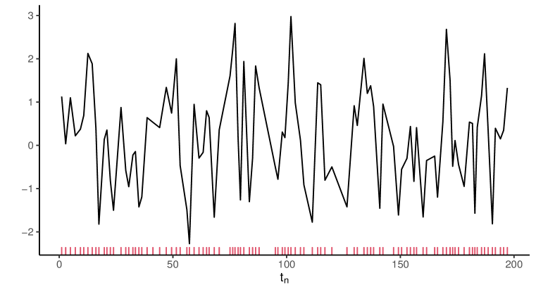
Figure 1: IMA trajectory example with $\theta=0.5$, $\sigma^{2}=1$ and $\textrm{N}=100$. On the bottom, we found the tick marks of irregularly spaced times.

4.1 ML estimators

Let $\hat{\theta}_{m}^{\textrm{MLE}}$ be the ML estimation and $\widehat{\textrm{se}}(\hat{\theta}_{m}^{\textrm{MLE}})$ be the estimated standard error for the $m$-th trajectory. The standard error is estimated by curvature of the likelihood surface at $\hat{\theta}_{m}^{\textrm{MLE}}$. The mean value of the M maximum likelihood estimations is computed as,

$$\hat{\theta}^{\textrm{MLE}}=\frac{1}{\textrm{M}}\sum_{m=1}^{\textrm{M}}\hat{\theta}_{m}^{\textrm{MLE}}\quad\textrm{and}\quad\widehat{\textrm{se}}(\hat{\theta}^{\textrm{MLE}})=\frac{1}{\textrm{M}}\sum_{m=1}^{\textrm{M}}\widehat{\textrm{se}}(\hat{\theta}_{m}^{\textrm{MLE}}).$$

4.2 Bootstrap estimators

For each trajectory, we simulated $\textrm{B}=500$ bootstrap trajectories represented by $\{\{\textrm{S}_{m,b}\}_{b=1}^{\textrm{B}}\}_{m=1}^{\textrm{M}}$. Then, the sequence $\{\{\hat{\theta}_{m,b}^{\textrm{b}}\}_{b=1}^{\textrm{B}}\}_{m=1}^{\textrm{M}}$ (the ML estimations) is obtained. The bootstrap estimation and their estimated variance error are defined as

$$\hat{\theta}_{m}^{\textrm{b}}=\frac{1}{\textrm{B}}\sum_{b=1}^{\textrm{B}}\hat{\theta}_{m,b}^{\textrm{b}}\quad\textrm{and}\quad\widehat{\textrm{se}}^{2}(\hat{\theta}_{m}^{\textrm{b}})=\frac{1}{\textrm{B}-1}\sum_{b=1}^{\textrm{B}}(\hat{\theta}_{m,b}^{\textrm{b}}-\hat{\theta}_{m}^{\textrm{b}})^{2},$$

for $m=1,\ldots,\textrm{M}$. Finally, the mean value of the M bootstrap estimations is given by

$$\hat{\theta}^{\textrm{b}}=\frac{1}{\textrm{M}}\sum_{m=1}^{\textrm{M}}\hat{\theta}_{m}^{\textrm{b}}\quad\textrm{and}\quad\widehat{\textrm{se}}(\hat{\theta}^{\textrm{b}})=\frac{1}{\textrm{M}}\sum_{m=1}^{\textrm{M}}\widehat{\textrm{se}}(\hat{\theta}_{m}^{\textrm{b}}).$$

4.3 Performance measures

Besides, as a measure of the estimator performance, the Root Mean Squared Error (RMSE), and the Coefficient of Variation (CV) are considered. Recall that in this case the RMSE and the CV may be written as

$$\textrm{RMSE}_{\hat{\theta}^{\textrm{MLE}}}=(\widehat{\textrm{se}}(\hat{\theta}^{\textrm{MLE}})^{2}+\textrm{bias}_{\hat{\theta}^{\textrm{MLE}}}^{2})^{\nicefrac{{1}}{{2}}},\;\textrm{and}$$

$$\textrm{CV}_{\hat{\theta}^{\textrm{MLE}}}=\frac{\widehat{\textrm{se}}(\hat{\theta}^{\textrm{MLE}})}{\left|\hat{\theta}^{\textrm{MLE}}\right|},$$

where $\textrm{bias}_{\hat{\theta}^{\textrm{MLE}}}=\hat{\theta}^{\textrm{MLE}}-\theta$. Finally, an approximate variance estimator is given by

$$\widetilde{\textrm{se}}^{2}(\hat{\theta}^{\textrm{MLE}})=\frac{1}{\textrm{M}-1}\sum_{m=1}^{\textrm{M}}(\hat{\theta}_{m}^{\textrm{MLE}}-\hat{\theta}^{\textrm{MLE}})^{2}.$$

$\textrm{RMSE}_{\hat{\theta}^{\textrm{b}}}$, $\textrm{CV}_{\hat{\theta}^{\textrm{b}}}$, $\textrm{bias}_{\hat{\theta}^{\textrm{b}}}$ and $\widetilde{\textrm{se}}^{2}(\hat{\theta}^{\textrm{b}})$ for the bootstrap case are defined analogously. Figure 2 shows the workflow of the simulation study.

Figure 2: General scheme of Monte Carlo study. Here, we show how we got the pairs $\{\hat{\theta}_{m}^{\textrm{mle}},\hat{\textrm{se}}(\hat{\theta}_{m}^{\textrm{mle}})\}_{m=1}^{\textrm{M}}$ and $\{\hat{\theta}_{m}^{\textrm{b}},\hat{\textrm{se}}(\hat{\theta}_{m}^{\textrm{b}})\}_{m=1}^{\textrm{M}}$ for each trajectory.

Next, the results for the irregularly spaced time case are reported (see Appendix D for the regularly spaced case). First, the simulated finite sample distributions for maximum likelihood and bootstrap estimators are shown. Second, the measures of performance for both estimators, are shown. Separately, the Monte Carlo Error (MCE) is estimated for every simulation via asymptotic theory (see, Koehler et al., 2009),

$$\frac{\widetilde{\textrm{se}}(\hat{\theta}^{\textrm{MLE}})}{\sqrt{M}},$$

and the maximum value is reported in each table. The MCE is a estimation of the standard deviation of the Monte Carlo estimator, taken across repetitions of the simulation, where each simulation is based on the same design and consists of $M$ replications.

4.4 Finite sample distributions for ML and bootstrap estimators

In Figure 3, the simulated finite sample distributions for maximum likelihood and bootstrap estimators are reported. Observe that both estimators behave well in these Monte Carlo experiments. They seem to be unbiased since the mean of the estimated values are close to their theoretical counterparts. However, for small values of $\theta_{0}$, the estimates exhibit greater variability.

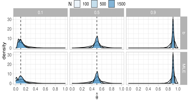
Figure 3: Simulated finite sample distributions. On the top, the MLE case. On the bottom, the bootstrap case.

Tables 1 and 2 exhibit the performance measures of the estimators, for maximum likelihood and bootstrap methods, respectively. Bias and variance are smaller when N increases as expected. Both methods provide good estimations for the standard error. Also, the irregularly spaced times seem to increase the estimation variability. In Appendix D, it is presented the regularly spaced times case. In this case, the IMA model is reduced to the conventional MA model, and the results are equally consistent.

Table 1: Monte Carlo results for the ML estimator with irregularly spaced times. The MCE estimated is $0.005$.

N	$\theta_{0}$	$\hat{\theta}^{\textrm{MLE}}$	$\widehat{\textrm{se}}(\hat{\theta}^{\textrm{MLE}})$	$\widetilde{\textrm{se}}(\hat{\theta}^{\textrm{MLE}})$	$\textrm{bias}_{\hat{\theta}^{\textrm{MLE}}}$	$\textrm{RMSE}_{\hat{\theta}^{\textrm{MLE}}}$	$\textrm{CV}_{\hat{\theta}^{\textrm{MLE}}}$
$100$	$0.1$	$0.132$	$0.184$	$0.135$	$0.032$	$0.186$	$1.389$
	$0.5$	$0.486$	$0.134$	$0.144$	$-0.014$	$0.135$	$0.276$
	$0.9$	$0.893$	$0.051$	$0.055$	$-0.007$	$0.052$	$0.057$
$500$	$0.1$	$0.100$	$0.093$	$0.074$	$0.000$	$0.093$	$0.930$
	$0.5$	$0.498$	$0.058$	$0.059$	$-0.002$	$0.058$	$0.117$
	$0.9$	$0.899$	$0.022$	$0.022$	$-0.001$	$0.022$	$0.024$
$1500$	$0.1$	$0.097$	$0.056$	$0.050$	$-0.003$	$0.056$	$0.574$
	$0.5$	$0.499$	$0.034$	$0.034$	$-0.001$	$0.034$	$0.068$
	$0.9$	$0.900$	$0.012$	$0.012$	$0.000$	$0.012$	$0.014$

Table 2: Monte Carlo results for the bootstrap estimator with irregularly spaced times. The MCE estimated is $0.005$.

N	$\theta_{0}$	$\hat{\theta}^{\textrm{b}}$	$\widehat{\textrm{se}}(\hat{\theta}^{\textrm{b}})$	$\widetilde{\textrm{se}}(\hat{\theta}^{\textrm{b}})$	$\textrm{bias}_{\hat{\theta}^{\textrm{b}}}$	$\textrm{RMSE}_{\hat{\theta}^{\textrm{b}}}$	$\textrm{CV}_{\hat{\theta}^{\textrm{b}}}$
$100$	$0.1$	$0.167$	$0.136$	$0.098$	$0.067$	$0.151$	$0.811$
	$0.5$	$0.473$	$0.140$	$0.139$	$-0.027$	$0.143$	$0.296$
	$0.9$	$0.887$	$0.055$	$0.056$	$-0.013$	$0.056$	$0.062$
$500$	$0.1$	$0.111$	$0.069$	$0.059$	$0.011$	$0.070$	$0.626$
	$0.5$	$0.496$	$0.059$	$0.059$	$-0.004$	$0.059$	$0.118$
	$0.9$	$0.898$	$0.022$	$0.023$	$-0.002$	$0.022$	$0.024$
$1500$	$0.1$	$0.099$	$0.047$	$0.043$	$-0.001$	$0.047$	$0.474$
	$0.5$	$0.498$	$0.034$	$0.033$	$-0.002$	$0.034$	$0.068$
	$0.9$	$0.900$	$0.012$	$0.012$	$0.000$	$0.012$	$0.014$

A second simulation experiment is performed in order to assess the performance of the CARMA$(p,q)$ model in fitting an IMA simulated process. The CARMA models has been generally used to fit irregularly sampled time series. However, as mentioned previously, the CARMA models are restricted to $p>q$, so the IMA model is not a particular case of the CARMA model (see, Phadke1974; Thornton and Chambers, 2013). For this reason, it is interesting to evaluate whether a CARMA model can properly fit an IMA process.

In this experiment, we generate 1000 sequences of the IMA process with two different lengths and four different values of the $\theta$ parameter. The irregular times were generated using a mixture of two exponential distributions with $130$ and $6.5$ as the mean of each exponential distribution and $0.15$ and $0.85$ as their respective weights. We chose this distribution of times in order to obtain large time gaps, which can be an issue when a model assumes continuous time.

In order to fit the CARMA model we use the function carma of the growth package of R. In addition, we opted to use the CARMA$(2,1)$ model since it is the most parsimonious CARMA model with a moving average component that can be fitted. Finally, we used the Root mean squared error as the goodness-of-fit measure. In table 9 we present the Monte Carlo results of this experiment. Note that the IMA model consistently outperforms the CARMA$(2,1)$ model. In particular, for large values of $\theta$ and $N$ the IMA model have almost 100% of success rate when selecting the model with lowest MSE. This result is relevant because when using the -2 log likelihood as a goodness-of-fit measure we are not penalizing by the number of parameters and anyways the IMA model has better performance than the CARMA model. In Appendix E, we uses other goodness-of-fit measures such as the Akaike Criterion and the -2 log likelihood. Considering these criteria, the IMA model also fits the simulated processes better than the CARMA$(2,1)$ model in most cases.

Table 3: Monte Carlo results of the experiment to compare the performance of the IMA and CARMA(2,1) models in fitting IMA model. The goodness of fit measure estimated from both models is the Root Mean Squared Error.

N	$\theta_{0}$	$\hat{\theta}$	$\widehat{\textrm{se}}(\hat{\theta})$	MSE_IMA	SD(MSE_IMA)	MSE_C21	SD(MSE_C21)	% Success
$300$	0.95	0.9437	0.0568	0.8383	0.0440	0.9154	0.0554	0.9880
	0.9	0.8912	0.0534	0.8815	0.0422	0.9272	0.0501	0.9550
	0.7	0.6762	0.1171	0.9277	0.0398	0.9432	0.0421	0.8240
	0.5	0.4900	0.1346	0.9427	0.0381	0.9496	0.0416	0.6220
$1000$	0.95	0.9464	0.0473	0.8385	0.0336	0.9200	0.0497	0.9970
	0.9	0.8971	0.0399	0.8818	0.0332	0.9289	0.0435	0.9970
	0.7	0.6924	0.0675	0.9311	0.0329	0.9456	0.0355	0.9620
	0.5	0.4949	0.0737	0.9463	0.0324	0.9541	0.0340	0.8980

4.5 Non-Gaussian errors

There are many applications where Gaussian assumption is misspecified, but it is assumed in the likelihood to obtain the ML estimators. These estimators are commonly known as quasi-ML estimators or QMLE.

This section shows the performance measures for the QMLE in a Monte Carlo experiment where it is simulated trajectories of the IMA model with non-Gaussian errors exploiting its constructionist viewpoint. First, it is used a Student distribution with shape parameter 7 (degree of freedom). Second, a Generalized error distribution with shape parameter 1.28 (heavy tails) is used. Both distribution are standardized according to specifications used by Ghalanos2020.

Tables 4 and 5 display the results obtained for Student and Generalized errors, respectively. In both cases, the performance obtained for the QMLE is very similar to the performance obtained for the MLE presented in Table 1 (Gaussian case). This suggests that QML estimators are robust to deviations from Gaussianity.

Table 4: Monte Carlo results for the QML estimator with irregularly spaced times and Student errors with shape parameter $7$. The MCE estimated is $0.004$.

N	$\theta_{0}$	$\hat{\theta}^{\textrm{MLE}}$	$\widehat{\textrm{se}}(\hat{\theta}^{\textrm{MLE}})$	$\widetilde{\textrm{se}}(\hat{\theta}^{\textrm{MLE}})$	$\textrm{bias}_{\hat{\theta}^{\textrm{MLE}}}$	$\textrm{RMSE}_{\hat{\theta}^{\textrm{MLE}}}$	$\textrm{CV}_{\hat{\theta}^{\textrm{MLE}}}$
$100$	$0.1$	$0.126$	$0.183$	$0.133$	$0.026$	$0.185$	$1.452$
	$0.5$	$0.488$	$0.138$	$0.140$	$-0.012$	$0.138$	$0.283$
	$0.9$	$0.897$	$0.050$	$0.054$	$-0.003$	$0.050$	$0.055$
$500$	$0.1$	$0.098$	$0.099$	$0.075$	$-0.002$	$0.099$	$1.012$
	$0.5$	$0.495$	$0.060$	$0.063$	$-0.005$	$0.060$	$0.122$
	$0.9$	$0.899$	$0.022$	$0.022$	$-0.001$	$0.022$	$0.024$
$1500$	$0.1$	$0.097$	$0.056$	$0.050$	$-0.003$	$0.056$	$0.575$
	$0.5$	$0.498$	$0.034$	$0.035$	$-0.002$	$0.034$	$0.069$
	$0.9$	$0.900$	$0.012$	$0.013$	$0.000$	$0.012$	$0.014$

Table 5: Monte Carlo results for the QML estimator with irregularly spaced times and Generalized errors with shape parameter $1.28$. The MCE estimated is $0.004$.

N	$\theta_{0}$	$\hat{\theta}^{\textrm{MLE}}$	$\widehat{\textrm{se}}(\hat{\theta}^{\textrm{MLE}})$	$\widetilde{\textrm{se}}(\hat{\theta}^{\textrm{MLE}})$	$\textrm{bias}_{\hat{\theta}^{\textrm{MLE}}}$	$\textrm{RMSE}_{\hat{\theta}^{\textrm{MLE}}}$	$\textrm{CV}_{\hat{\theta}^{\textrm{MLE}}}$
$100$	$0.1$	$0.128$	$0.193$	$0.135$	$0.028$	$0.195$	$1.503$
	$0.5$	$0.491$	$0.136$	$0.139$	$-0.009$	$0.136$	$0.276$
	$0.9$	$0.896$	$0.050$	$0.053$	$-0.004$	$0.051$	$0.056$
$500$	$0.1$	$0.102$	$0.096$	$0.077$	$0.002$	$0.096$	$0.945$
	$0.5$	$0.497$	$0.060$	$0.062$	$-0.003$	$0.060$	$0.120$
	$0.9$	$0.899$	$0.022$	$0.021$	$-0.001$	$0.022$	$0.024$
$1500$	$0.1$	$0.098$	$0.055$	$0.050$	$-0.002$	$0.055$	$0.561$
	$0.5$	$0.500$	$0.034$	$0.034$	$0.000$	$0.034$	$0.068$
	$0.9$	$0.900$	$0.012$	$0.012$	$0.000$	$0.012$	$0.014$

5 Applications

This section illustrates the application of the proposed time series methodology to two real-life datasets. The first example is concerned with medical data whereas in the second application is described the analysis of light curves in astronomy.

5.1 Lung function of an asthma patient

Belcher et al. (1994) analyzed measurements of the lung function of an asthma patient. The observations are collected mostly at 2 hour time intervals but with irregular gaps (see the unequal spaced of tick marks in Figure 4). However, as it was shown in Wang (2013), the trend component (obtained by decomposing original time series into trend, seasonal, and irregular components via the Kalman smoother) exhibits structural changes after 100$th$ observation. Thus, the first 100 observations are considered here to analyze such a phenomenon. Below, the ML and bootstrap estimates are reported along with their respective estimated standard errors. Note that the estimates are significant at the 5% significance level.

$$\hat{\theta}^{\textrm{MLE}}=0.853\quad\widehat{\textrm{se}}(\hat{\theta}^{\textrm{MLE}})=0.069\quad\hat{\sigma}_{\textrm{MLE}}^{2}=258.286\quad\widehat{\textrm{se}}(\hat{\sigma}_{\textrm{MLE}}^{2})=36.537$$

$$\hat{\theta}^{\textrm{b}}=0.841\quad\widehat{\textrm{se}}(\hat{\theta}^{\textrm{b}})=0.077\quad\hat{\sigma}_{\textrm{b}}^{2}=259.270\quad\widehat{\textrm{se}}(\hat{\sigma}_{\textrm{b}}^{2})=32.662$$

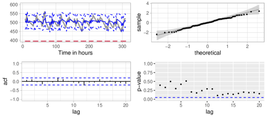
Figure 4: On the left-top, the lung function of an asthma patient with the predicted values and their respective variability bands. On the right-top, quantile-quantile plot of the standardized residuals with normality reference bands. In this case, we use $\hat{\theta}^{\textrm{MLE}}$. On the bottom-left, the autocorrelation function estimated of the standardized residuals. On the bottom-right, the Ljung-Box test for randomness of the standardized residuals.

From Figure 4, the fit seems adequate. Also, the standardized residuals seem to follow a standard normal distribution (Nair1982). Figure 4 shows the ACF estimated and the results from a Ljung-Box test for the standardized residuals. Observe that the residuals satisfy the white noise test at the $5$% significance level. Note that, since the standardized residuals are assumed to be realizations of a random sample, its correlation structure does not depend on the irregularly spaced between observations. Thus, unlike the original time series, the ACF and the Ljung-Box test can be applied to the standardized residuals.

Estimated mean squared errors for the one-step predictors are presented in Figure 5 under the IMA and the MA model. Notice that under the IMA model, the MSE is smaller when the time distances become smaller while, under the MA model, the MSE is constant regardless of the size of these distances. Also, it is important to consider that both MSE, on average, exhibit similar behavior.

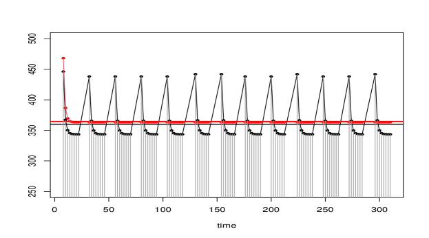
Figure 5: Estimated mean squared errors for the lung function data. Black line represent MSE under the IMA model while red line represent MSE under the MA model. Horizontal lines are their corresponding averages.

5.2 Light curves

In astronomy it is common to find time series measured at irregular times. These temporal data generally correspond to the brightness of an astronomical object over time. The time sequence of measurements of the brightness of an astronomical object is known as the light curve of this object. In this example, the IMA model is fitted to the light curve of a Blazar object. Blazar objects are characterized by stochastics signals in its light curves. The light curve used in this example was observed with the Zwicky Transient Facility (ZTF, Bellm (2018)) survey (coded as ZTF18abvfmot). The observations from the ZTF survey were processed by the ALeRCE broker (ALeRCE). The light curve has 105 observations taken over a range of approximately 480 days. Before fitting the model, we perform a transformation of the time series in order to stabilize its variance. Hereafter, the Blazar time series will be referred to as the light curve.

The IMA model parameters $\theta$ and $\sigma^{2}$ estimated in the Blazar light curve by the maximum likelihood and bootstrap methods, and their respective estimated standard errors are the following,

$$\hat{\theta}^{\textrm{MLE}}=0.815\quad\widehat{\textrm{se}}(\hat{\theta}^{\textrm{MLE}})=0.085\quad\hat{\sigma}_{\textrm{MLE}}^{2}=0.593\quad\widehat{\textrm{se}}(\hat{\sigma}_{\textrm{MLE}}^{2})=0.084$$

$$\hat{\theta}^{\textrm{b}}=0.802\quad\widehat{\textrm{se}}(\hat{\theta}^{\textrm{b}})=0.089\quad\hat{\sigma}_{\textrm{b}}^{2}=0.581\quad\widehat{\textrm{se}}(\hat{\sigma}_{\textrm{b}}^{2})=0.058$$

Note that, the parameter $\theta$ estimated by both methods is significant greater than zero at the 5% significance level. Consequently, the IMA model detect a significant correlation structure in the Blazar ligth curve. To assess whether the model is able to explain the entire correlation structure of the data, a residual analysis is performed. Figure 6 shows the residuals of the model. According to the figure, residuals are normally distributed and are uncorrelated. Therefore, the IMA model here removes the serial autocorrelation.

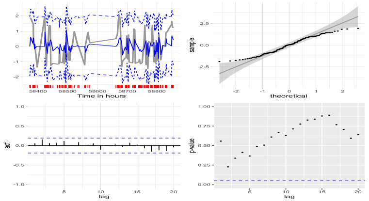
Figure 6: Analysis of the residuals of the IMA model fitted to the Blazar light curve.

To assess the goodness of fit of the IMA model on the Blazar light curve, we estimate its mean square errors for the one-step predictors. We compare these estimates with the mean square errors obtained for the regular MA model. Note from Figure 7 that the average of the MSE of both models are similar. However, as in the previous example, the MSE of the IMA model is smaller of the obtained with the MA model when the time gaps are smaller, while for large gaps the MA model have a smaller value of the MSE.

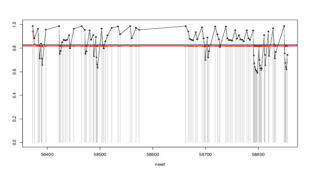
Figure 7: Estimated mean squared errors for the Blazar light curve. Black line represent MSE under the IMA model while red line represent MSE under the MA model. Horizontal lines are their corresponding averages.

6 Conclusions

This paper proposes an irregularly spaced first-order MA model that allows for the handling of first-order moving averages structures with irregularly spaced times. Its formal definition is provided and some of its statistical properties are studied. State space representations along with one-step linear predictors are also provided. Furthermore, the finite-sample performance of the proposed estimation methods is investigated by means of Monte Carlo simulations for both Gaussian and non-Gaussian distributions errors. The proposed methods display very good estimation performance in all the cases investigated. The performance of the proposed IMA model is also compared to the CARMA processes. Finally, the practical application of the proposed methodology is illustrated by means of two real-life data examples involving medical and astronomical time series.

Appendix A Constructionist viewpoint

Details about defining an IMA model from the constructionist viewpoint are discussed next. The main idea is to specify the IMA process as a function of other (often simpler) stochastic processes. Let $\{\zeta_{t_{n}}\}_{n\geq 1}$ be uncorrelated random variables each with mean 0 and variance 1. Now, consider

$$X_{t_{1}}=\nu_{1}^{\nicefrac{{1}}{{2}}}\zeta_{t_{1}},$$

$$X_{t_{n+1}}=\nu_{n+1}^{\nicefrac{{1}}{{2}}}\zeta_{t_{n+1}}+\omega_{n}\nu_{n}^{\nicefrac{{1}}{{2}}}\zeta_{t_{n}},\quad\textrm{for}\;n\geq 1,$$

where $\{\nu_{n}\}_{n\geq 1}$ and $\{\omega_{n}\}_{n\geq 1}$ are time-varying sequences that characterize the moments of the process. Thus, for $n\geq 1$, we have $\textrm{E}(X_{t_{n}})=0$,

$$\textrm{Var}(X_{t_{1}})=\nu_{1},\;\textrm{Var}(X_{t_{n+1}})=\nu_{n+1}+\omega_{n}^{2}\nu_{n},\;\textrm{and}$$

$$\textrm{Cov}(X_{t_{n}},X_{t_{n+k}})=\begin{cases}\omega_{n}\nu_{n},&k=1,\\ 0,&k\geq 2.\end{cases}$$

The main goal is to find $\{\nu_{n}\}_{n\geq 1}$ and $\{\omega_{n}\}_{n\geq 1}$ so that $\{X_{t_{n}}\}_{n\geq 1}$ be a stationary process. For this, we need that, for $n\geq 1$, $\textrm{Var}(X_{t_{n+1}})=\textrm{Var}(X_{t_{1}})=\gamma_{0}$ and $\textrm{Cov}(X_{t_{n}},X_{t_{n+1}})=\gamma_{1,\Delta_{n+1}}$ with $\gamma_{1,\Delta_{n+1}}$ a function of $\Delta_{n+1}=t_{n+1}-t_{n}$. Thus,

$$\nu_{n+1}+\omega_{n}^{2}\nu_{n}=\nu_{1}=\gamma_{0}\;\textrm{and}$$

$$\omega_{n}\nu_{n}=\gamma_{1,\Delta_{n+1}}\quad\textrm{for}\;n\geq 1.$$

From these equations, we obtain

$$\omega_{n}=\frac{\gamma_{1,\Delta_{n+1}}}{\nu_{n}}\quad\textrm{and}\quad\nu_{n+1}=\gamma_{0}-\frac{\gamma_{1,\Delta_{n+1}}^{2}}{\nu_{n}},\quad\textrm{with}\;\nu_{1}=\gamma_{0}.$$ (8)

Therefore, we can set a real-valued stationary process defining $\gamma_{0}$ and $\{\gamma_{1,\Delta_{n+1}}\}_{n\geq 1}$ suitably, that is, in such a way that $\nu_{n}>0$, for all $n$. Proposition 1 shows that setting

$$\gamma_{0}=\sigma^{2}(1+\theta^{2})\qquad\textrm{and}\qquad\gamma_{1,\Delta_{n+1}}=\sigma^{2}\theta^{\Delta_{n+1}}\quad\textrm{for}\;n\geq 1,$$

with $\sigma^{2}>0$ and $0\leq\theta<1$, the general backward continued fraction $\{\nu_{n}\}_{n\geq 1}$ is a strictly positive sequence. Hence, $\{X_{t_{n}}\}_{n\geq 1}$ is a well defined real-valued stationary stochastic process.

Proposition 1.

Consider a real-valued sequence $\{\nu_{n}\}_{n\geq 1}$ as defined in (8). If $\gamma_{0}>0$, and for $n\geq 1$, $\left(\frac{\gamma_{1,\Delta_{n+1}}}{\gamma_{0}}\right)^{2}\leq\nicefrac{{1}}{{4}}$ with $\gamma_{1,\Delta_{n+1}}\neq 0$, then $\{\nu_{n}\}_{n\geq 1}$ is a strictly positive sequence.

Proof.

The $(n+1)$-th convergent of the general backward continued fraction, $\{\nu_{n}\}_{n\geq 1}$, is defined as

$$\nu_{n+1}=\left[\gamma_{0}+\frac{-\gamma_{1,\Delta_{2}}^{2}}{\gamma_{0}+}\frac{-\gamma_{1,\Delta_{3}}^{2}}{\gamma_{0}+}\cdots\frac{-\gamma_{1,\Delta_{n+1}}^{2}}{\gamma_{0}}\right]_{b}=\gamma_{0}+\cfrac{-\gamma_{1,\Delta_{n+1}}^{2}}{\gamma_{0}+\cfrac{-\gamma_{1,\Delta_{n}}^{2}}{\gamma_{0}+\cfrac{\ddots}{\gamma_{0}+\cfrac{-\gamma_{1,\Delta_{2}}^{2}}{\gamma_{0}}}}}.$$

Thus, few convergent are

$$\nu_{2} =\left[\gamma_{0}+\frac{-\gamma_{1,\Delta_{2}}^{2}}{\gamma_{0}+}\right]_{b}=\frac{\gamma_{0}^{2}-\gamma_{1,\Delta_{2}}^{2}}{\gamma_{0}},$$

$$\nu_{3} =\left[\gamma_{0}+\frac{-\gamma_{1,\Delta_{2}}^{2}}{\gamma_{0}+}\frac{-\gamma_{1,\Delta_{3}}^{2}}{\gamma_{0}+}\right]_{b}=\frac{\gamma_{0}^{3}-\gamma_{0}\gamma_{1,\Delta_{2}}^{2}-\gamma_{0}\gamma_{1,\Delta_{3}}^{2}}{\gamma_{0}^{2}-\gamma_{1,\Delta_{2}}^{2}},$$

$$\nu_{4} =\left[\gamma_{0}+\frac{-\gamma_{1,\Delta_{2}}^{2}}{\gamma_{0}+}\frac{-\gamma_{1,\Delta_{3}}^{2}}{\gamma_{0}+}\frac{-\gamma_{1,\Delta_{4}}^{2}}{\gamma_{0}+}\right]_{b}=\frac{\gamma_{0}^{4}-\gamma_{0}^{2}\gamma_{1,\Delta_{2}}^{2}-\gamma_{0}^{2}\gamma_{1,\Delta_{3}}^{2}-\gamma_{0}^{2}\gamma_{1,\Delta_{4}}^{2}+\gamma_{1,\Delta_{2}}^{2}\gamma_{1,\Delta_{4}}^{2}}{\gamma_{0}^{3}-\gamma_{0}\gamma_{1,\Delta_{2}}^{2}-\gamma_{0}\gamma_{1,\Delta_{3}}^{2}}.$$

The ratio for the general backward continued fraction, $\{\nu_{n}\}_{n\geq 1}$, is

$$\nu_{1}=\frac{P_{1}}{P_{0}}\;\textrm{and}\;\nu_{n+1}=\frac{P_{n+1}}{P_{n}},$$

for $n\geq 1$, where the sequence $\{P_{n}\}_{n\geq 0}$ is

$$P_{n+1}=\gamma_{0}P_{n}-\gamma_{1,\Delta_{n+1}}^{2}P_{n-1}$$

with $P_{1}=\gamma_{0}$ and $P_{0}=1$. This sequence is obtained by what is known as the Wallis-Euler recurrence relations (Loya, 2017). El-Mikkawy and Karawia (2006) proves that $P_{k}>0$, for $k=1,\ldots,n+1$, if and only if the matrix

$$\boldsymbol{\Gamma}_{n+1}=\begin{bmatrix}\gamma_{0}&\gamma_{1,\Delta_{2}}&\cdots&0&0\\ \gamma_{1,\Delta_{2}}&\gamma_{0}&\cdots&0&0\\ \vdots&\vdots&\ddots&\vdots&\vdots\\ 0&0&\cdots&\gamma_{0}&\gamma_{1,\Delta_{n+1}}\\ 0&0&\cdots&\gamma_{1,\Delta_{n+1}}&\gamma_{0}\end{bmatrix}$$

is positive definite with $\boldsymbol{\Gamma}_{1}=[\gamma_{0}]$. Further, they proved that $\det\boldsymbol{\Gamma}_{1}=P_{1}$ and $\det\boldsymbol{\Gamma}_{n+1}=P_{n+1}$.

Thus, from (2), if $\gamma_{0}>0$ and, for $n\geq 1$, $\left(\frac{\gamma_{1,\Delta_{n+1}}}{\gamma_{0}}\right)^{2}\leq\nicefrac{{1}}{{4}}$ with $\gamma_{1,\Delta_{n+1}}\neq 0$, then $\{\nu_{n}\}_{n\geq 1}$ is a strictly positive sequence. ∎

Appendix B Proof of $1<c_{n}(\theta)<2$ for $n\geq 1$

Consider the general backward continued fraction of the IMA model

$$c_{n}(\theta)=1+\theta^{2}-\frac{\theta^{2\Delta_{n}}}{c_{n-1}(\theta)},\quad n\geq 2,$$

with $c_{1}(\theta)=1+\theta^{2}$.

Proposition 2.

If $0\leq\theta<1$, and $\Delta_{n}\geq 1$, for all $n$, then

$$1\leq c_{n}(\theta)<2\quad\textrm{for}\quad n\geq 1.$$

Proof.

By induction. For $n=1$, we have straightly that $1\leq c_{1}(\theta)<2$. Now, consider (for $n\geq 2$) that $1\leq c_{n-1}(\theta)<2$ as the hypothesis. Then,

$$c_{n}(\theta)=1+\theta^{2}-\frac{\theta^{2\Delta_{n}}}{c_{n-1}(\theta)}<1+\theta^{2}=c_{1}(\theta)<2,$$

since ${\theta^{2\Delta_{n}}}/{c_{n-1}(\theta)}>0$. Also, since ${\theta^{2\Delta_{n}}}/{c_{n-1}(\theta)}<\theta^{2\Delta_{n}}$, then

$$c_{n}(\theta)=1+\theta^{2}-\frac{\theta^{2\Delta_{n}}}{c_{n-1}(\theta)}>1+\theta^{2}-\theta^{2\Delta_{n}}$$

but $\theta^{2\Delta_{n}}\leq\theta^{2}$ since $\Delta_{n}\geq 1$. Thus,

$$c_{n}(\theta)>1+\theta^{2}-\theta^{2\Delta_{n}}\geq 1$$

obtaining the desired result. ∎

Appendix C Innovations algorithm

Following (Brockwell and Davis, 1991, Proposition 5.2.2), we obtain the coefficients of $\hat{X}_{t_{n+1}}=\sum_{j=1}^{n}\theta_{nj}(X_{t_{n+1-j}}-\hat{X}_{t_{n+1-j}})$ through the next proposition.

Proposition 3.

If $\{X_{t_{n}}\}_{n\geq 1}$ has zero mean and $\textrm{E}(X_{t_{i}}X_{t_{j}})=\gamma(t_{i},t_{j})$, where the matrix $\left[\gamma(t_{i},t_{j})\right]_{i,j=1}^{n}$ is non-singular for each $n=1,2,\ldots$, then the one-step predictors $\hat{X}_{t_{n+1}}$, and their mean squared errors $\upsilon_{n+1}$, $n\geq 0$, are given by

$$\hat{X}_{t_{n+1}}=\begin{cases}0&\textrm{if}\qquad n=0,\\ \sum_{j=1}^{n}\theta_{nj}\left(X_{t_{n+1-j}}-\hat{X}_{t_{n+1-j}}\right)&\textrm{if}\qquad n\geq 1,\end{cases}$$

and

$$\begin{cases}\upsilon_{1}&=\gamma(t_{1},t_{1}),\\ \theta_{n,n-k}&=\upsilon_{k+1}^{-1}\left(\gamma(t_{n+1},t_{k+1})-\sum_{j=0}^{k-1}\theta_{k,k-j}\theta_{n,n-j}\upsilon_{j+1}\right),k=0,1,\ldots,n-1,\\ \upsilon_{n+1}&=\gamma(t_{n+1},t_{n+1})-\sum_{j=0}^{n-1}\theta_{n,n-j}^{2}\upsilon_{j+1}.\end{cases}$$

For the irregularly spaced first-order moving average process of general form we have,

$$\theta_{n,j} =0,\quad 2\leq j\leq n,$$

$$\theta_{n,1} =\upsilon_{n}^{-1}\gamma_{1,\Delta_{n+1}},$$

$$\upsilon_{n+1} =\gamma_{0}-\theta_{n,1}^{2}\upsilon_{n}=\gamma_{0}-\frac{\gamma_{1,\Delta_{n+1}}^{2}}{\upsilon_{n}},\;\textrm{and}\;\upsilon_{1}=\gamma_{0}.$$

Appendix D Measures of performance-regularly spaced case

In this section, the performance of irregularly spaced case for the ML and Bootstrap estimators is compared in the context of regularly spaced times. Tables 6 and 7 show the Monte Carlo results.

In addition, Table 6, also consider the asymptotic standard error for the ML estimator defined as the square root of

$$\textrm{se}^{2}(\hat{\theta}^{\textrm{MLE}})=\frac{1-\theta^{2}}{\textrm{N}}.$$

From these tables, notice that the Monte Carlo results for the regularly spaced time case exhibit a similar behavior as compared to the irregularly spaced time case.

Table 6: Monte Carlo results for the ML estimator with regularly spaced times. The MCE estimated is $0.003$.

N	$\theta_{0}$	$\hat{\theta}^{\textrm{MLE}}$	$\widehat{\textrm{se}}(\hat{\theta}^{\textrm{MLE}})$	$\widetilde{\textrm{se}}(\hat{\theta}^{\textrm{MLE}})$	$\textrm{se}(\hat{\theta}^{\textrm{MLE}})$	$\textrm{bias}_{\hat{\theta}^{\textrm{MLE}}}$	$\textrm{RMSE}_{\hat{\theta}^{\textrm{MLE}}}$	$\textrm{CV}_{\hat{\theta}^{\textrm{MLE}}}$
$100$	$0.1$	$0.108$	$0.103$	$0.087$	$0.099$	$0.008$	$0.103$	$0.952$
	$0.5$	$0.502$	$0.089$	$0.096$	$0.087$	$0.002$	$0.089$	$0.178$
	$0.9$	$0.910$	$0.051$	$0.055$	$0.044$	$0.010$	$0.052$	$0.056$
$500$	$0.1$	$0.097$	$0.045$	$0.044$	$0.044$	$-0.003$	$0.045$	$0.461$
	$0.5$	$0.499$	$0.039$	$0.039$	$0.039$	$-0.001$	$0.039$	$0.078$
	$0.9$	$0.901$	$0.020$	$0.021$	$0.019$	$0.001$	$0.020$	$0.022$
$1500$	$0.1$	$0.099$	$0.026$	$0.026$	$0.026$	$-0.001$	$0.026$	$0.261$
	$0.5$	$0.500$	$0.022$	$0.022$	$0.022$	$0.000$	$0.022$	$0.045$
	$0.9$	$0.901$	$0.011$	$0.011$	$0.011$	$0.001$	$0.011$	$0.013$

Table 7: Monte Carlo results for the bootstrap estimator with regularly spaced times. The MCE estimated is $0.003$.

N	$\theta_{0}$	$\hat{\theta}^{\textrm{b}}$	$\widehat{\textrm{se}}(\hat{\theta}^{\textrm{b}})$	$\widetilde{\textrm{se}}(\hat{\theta}^{\textrm{b}})$	$\textrm{bias}_{\hat{\theta}^{\textrm{b}}}$	$\textrm{RMSE}_{\hat{\theta}^{\textrm{b}}}$	$\textrm{CV}_{\hat{\theta}^{\textrm{b}}}$
$100$	$0.1$	$0.120$	$0.082$	$0.073$	$0.020$	$0.084$	$0.685$
	$0.5$	$0.502$	$0.093$	$0.099$	$0.002$	$0.093$	$0.186$
	$0.9$	$0.915$	$0.049$	$0.050$	$0.015$	$0.051$	$0.054$
$500$	$0.1$	$0.098$	$0.041$	$0.042$	$-0.002$	$0.042$	$0.422$
	$0.5$	$0.499$	$0.039$	$0.041$	$-0.001$	$0.039$	$0.079$
	$0.9$	$0.902$	$0.020$	$0.021$	$0.002$	$0.021$	$0.023$
$1500$	$0.1$	$0.098$	$0.026$	$0.026$	$-0.002$	$0.026$	$0.260$
	$0.5$	$0.500$	$0.022$	$0.023$	$0.000$	$0.022$	$0.045$
	$0.9$	$0.902$	$0.011$	$0.012$	$0.002$	$0.011$	$0.013$

Appendix E Measures of performance in comparison with CARMA(2,1) model

Table 8: Monte Carlo results of the experiment to compare the performance of the IMA and CARMA(2,1) models in fitting IMA model. The goodness of fit measure estimated from both models is the AIC.

N	$\theta_{0}$	$\hat{\theta}$	$\widehat{\textrm{se}}(\hat{\theta})$	AIC_IMA	SD(AIC_IMA)	AIC_C21	SD(AIC_C21)	% Success
$300$	0.95	0.9437	0.0568	399.4029	14.1419	416.4938	15.3710	0.9930
	0.9	0.8912	0.0534	407.1385	14.0296	419.1464	22.0460	0.9940
	0.7	0.6762	0.1171	414.5499	13.9158	421.0512	19.3402	0.9750
	0.5	0.4900	0.1346	416.5100	13.8214	421.8210	26.3998	0.9740
$1000$	0.95	0.9464	0.0473	1327.2653	43.8182	1383.1773	77.7452	0.9970
	0.9	0.8971	0.0399	1352.7468	44.0957	1387.5857	79.1279	0.9970
	0.7	0.6924	0.0675	1379.2990	44.4712	1393.3974	54.6430	0.9910
	0.5	0.4949	0.0737	1385.7829	44.4713	1395.4456	46.6157	0.9930

Table 9: Monte Carlo results of the experiment to compare the performance of the IMA and CARMA(2,1) models in fitting IMA model. The goodness of fit measure estimated from both models is the -2 Log-likelihood.

N	$\theta_{0}$	$\hat{\theta}$	$\widehat{\textrm{se}}(\hat{\theta})$	LL_IMA	SD(LL_IMA)	LL_C21	SD(LL_C21)	% Success
$300$	0.95	0.9437	0.0568	397.4049	14.0854	411.4988	15.2356	0.9860
	0.9	0.8912	0.0534	405.1405	13.9716	414.1514	21.9512	0.9470
	0.7	0.6762	0.1171	412.5519	13.8562	416.0562	19.2315	0.8050
	0.5	0.4900	0.1346	414.5120	13.7611	416.8260	26.3202	0.6730
$1000$	0.95	0.9464	0.0473	1325.2673	43.7576	1378.1823	77.6563	0.9970
	0.9	0.8971	0.0399	1350.7488	44.0343	1382.5907	79.0402	0.9970
	0.7	0.6924	0.0675	1377.3010	44.4091	1388.4024	54.5155	0.9600
	0.5	0.4949	0.0737	1383.7849	44.4089	1390.4506	46.4659	0.8920

Table 10: Monte Carlo results of the experiment to estimate the parameters of the IMA and CARMA(2,1) models in a simulated IMA process.

N	$\theta_{0}$	$\hat{\theta}$	$SD(\hat{\theta})$	$\hat{\phi_{1}^{C}}$	$SD(\hat{\phi_{1}^{C}})$	$\hat{\phi_{2}^{C}}$	$SD(\hat{\phi_{2}^{C}})$	$\hat{\theta_{1}^{C}}$	$SD(\hat{\theta_{1}^{C}})$
$300$	0.95	0.9437	0.0568	1.9772	2.4118	4.4998	2.0976	2.4048	5.2211
	0.9	0.8912	0.0534	1.9880	2.6548	4.3337	2.2127	2.1737	4.4533
	0.7	0.6762	0.1171	1.1625	3.6967	3.2940	2.7077	5.5312	13.1653
	0.5	0.4900	0.1346	1.6704	3.5028	2.8492	2.5655	4.1638	9.0002
$1000$	0.95	0.9464	0.0473	2.9784	2.2235	5.5765	1.9523	2.1122	5.9226
	0.9	0.8971	0.0399	3.2768	2.3768	5.5184	2.1549	1.4643	3.4077
	0.7	0.6924	0.0675	3.7004	3.2235	5.1538	2.4396	1.1568	3.4549
	0.5	0.4949	0.0737	3.5409	3.5898	4.4348	2.6495	1.4821	3.6772

References

• Adorf (1995) H. M. Adorf. (1995). Interpolation of irregularly sampled data series–a survey. In R. A. Shaw, H. E. Payne, and J. J. E. Hayes, editors, Astronomical data analysis software and systems IV, Vol. 77, ASP Conference Series. Astronomical Society of the Pacific, , pp. 460–463.
• Azencott and Dacunha-Castelle (1986) R. Azencott and D. Dacunha-Castelle. (1986). Series of irregular observations: forecasting and model building. Applied Probability, A Series of the Applied Probability Trust. Springer-Verlag New York, Inc., New York, New York.
• Babu and Mahabal (2016) G. J. Babu and A. Mahabal. (2016). Skysurveys, light curves and statistical challenges. International Statistical Review 84, 506–527.
• Belcher et al. (1994) J. Belcher, J. S. Hampton, and G. Tunnicliffe Wilson. (1994). Parametrization of continuous time autoregressive models for irregularly sampled time series data. Journal of the Royal Statistical Society, Series B (Methodological) 56, 141–155.
• Bellm (2018) E. C. Bellm. (2018). The zwicky transient facility: System overview, performance, and first results. Publications of the Astronomical Society of the Pacific 131, 018002.
• Bose (1990) A. Bose. (1990). Bootstrap in moving average models. Annals of the Institute of Statistical Mathematics 42, 753–768.
• Bowman and Azzalini (1997) A.W. Bowman and A. Azzalini. (1997). Applied smoothing techniques for data analysis: the kernel approach with S-Plus illustrations. Number 18 in Oxford Statistical Science Series. Oxford University Press, .
• Box et al. (2016) G. E. P. Box, G. M. Jenkins, G. C. Reinsel, and G. M. Ljung. (2016). Time series analysis: forecasting and control. Wiley Series in Probability and Statistics. John Wiley & Sons, Inc., Hoboken, New Jersey.
• Brockwell and Davis (1991) P. J. Brockwell and R. A. Davis. (1991). Time series: theory and methods. Springer Series in Statistics. Springer Science +Business Media, LLC, New York, USA.
• Caceres et al. (2019) G. A Caceres, E. D. Feigelson, G. J. Babu, N. Bahamonde, A. Christen, K. Bertin, C. Meza, and M. Curé. (2019). Autoregressive planet search: Methodology. The Astronomical Journal 158, 57.
• Corduas and Piccolo (2008) M. Corduas and D. Piccolo. (2008). Time series clustering and classification by the autoregressive metric. Computational Statistics & Data Analysis 52, 1860 – 1872.
• Dunsmuir (1983) W. Dunsmuir. (1983). A central limit theorem for estimation in gaussian stationary time series observed at unequally spaced times. Stochastic Processes and their Applications 14, 279–295.
• Edelmann et al. (2019) D. Edelmann, K. Fokianos, and M. Pitsillou. (2019). An updated literature review of distance correlation and its applications to time series. International Statistical Review 87, 237–262.
• El-Mikkawy and Karawia (2006) M. El-Mikkawy and A. Karawia. (2006). Inversion of general tridiagonal matrices. Applied Mathematics Letters 19, 712–720.
• Elorrieta et al. (2019) F. Elorrieta, S. Eyheramendy, and W. Palma. (2019). Discrete-time autoregressive model for unequally spaced time-series observations. A&A 627, A120.
• Eyheramendy et al. (2016) S. Eyheramendy, F. Elorrieta, and W. Palma. (2016). An autoregressive model for irregular time series of variable stars. Proceedings of the International Astronomical Union 12, 259–262.
• Eyheramendy et al. (2018) S. Eyheramendy, F. Elorrieta, and W. Palma. (2018). An irregular discrete time series model to identify residuals with autocorrelation in astronomical light curves. Monthly Notices of the Royal Astronomical Society 481, 4311–4322.
• Hamilton (1994) J. D. Hamilton. (1994). Time series analysis. Princeton University Press, Princeton, New Jersey.
• Hand (2008) D. J. Hand. (2008). Statistical analysis and modelling of spatial point patterns by janine illian, antti penttinen, helga stoyan, dietrich stoyan. International Statistical Review 76, 458–458.
• Hannan (1970) E. J. Hannan. (1970). Multiple time series. Wiley Series in Probability and Mathematical Statistics. John Wiley & Sons, Inc., .
• Harvey (1989) A. C. Harvey. (1989). Forecasting, structural time series models and the Kalman filter. Cambridge University Press, .
• Harvill et al. (2013) J. L. Harvill, N. Ravishanker, and B. K. Ray. (2013). Bispectral-based methods for clustering time series. Computational Statistics & Data Analysis 64, 113 – 131.
• Ismail and Muldoon (1991) M. E. H. Ismail and M. E. Muldoon. (1991). A discrete approach to monotonicity of zeros of orthogonal polynomials. Transactions of the American Mathematical Society 323, 65–78.
• Kiliç (2008) E. Kiliç. (2008). Explicit formula for the inverse of a tridiagonal matrix by backward continued fractions. Applied Mathematics and Computation 197, 345–357.
• Koehler et al. (2009) E. Koehler, E. Brown, and S. J. Haneuse. (2009). On the assessment of Monte Carlo error in simulation-based statistical analyses. 63, 155–162.
• Loya (2017) P. Loya. (2017). Amazing and aesthetic aspects of analysis. Springer, .
• Muñoz et al. (1992) A. Muñoz, V. Carey, J. P. Schouten, M. Segal, and B. Rosner. (1992). A parameteric family of correlation structures for the analysis of longitudinal data. Biometrics 48, 733–742.
• Mudelsee (2014) M. Mudelsee. (2014). Climate time series analysis: classical statistical and bootstrap methods Vol. 51, Atmospheric and Oceanographic Sciences Library. Springer International Publishing, .
• Parzen (1963) E. Parzen. (1963). On spectral analysis with missing observations and amplitude modulation. Sankhyā: The Indian Journal of Statistics, Series A (1961–2002) 25, 383–392.
• Parzen (1984) E. Parzen, editor. Time series analysis of irregularly observed data Vol. 25, Lecture Notes in Statistics(1984). Springer-Verlag. Proceedings of a Symposium held at Texas A & M University, College Station, Texas, February 10–13, 1983.
• Podgorski (2014) K. Podgorski. (2014). Advances in machine learning and data mining for astronomy edited by michael j. way, jeffrey d. scargle, kamal m. ali, and ashok n. srivstava. International Statistical Review 82, 153–154.
• Reinsel and Wincek (1987) March G. C. Reinsel and M. A. Wincek. (1987). Asymptotic distribution of parameter estimators for nonconsecutively observed time series. Biometrika 74, 115–124.
• Robinson (1977) P. M. Robinson. (1977). Estimation of a time series model from unequally spaced data. Stochastic Processes and their Applications 6, 9–24.
• Shumway and Stoffer (2017) R. H. Shumway and D. S. Stoffer. (2017). Time series analysis and its applications with R examples. Springer Texts in Statistics. Springer International Publishing AG, .
• Spanos (1999) A. Spanos. (1999). Probability theory and statistical inference: econometric modeling with observational data. Cambridge University Press, .
• Stout (1974) W. F. Stout. (1974). Almost sure convergence. Number 24 in Probability and Mathematical Statistics. Academic Press, Inc., .
• Thornton and Chambers (2013) M. A. Thornton and M. J. Chambers. (2013). Continuous-time autoregressive moving average processes in discrete time: representation and embeddability. Journal of Time Series Analysis 34, 552–561.
• Tómasson (2015) H. Tómasson. (2015). Some computational aspects of gaussian CARMA modelling. Statistics and Computing 25, 375–387.
• Wang (2013) Z. Wang. (2013). cts: An R package for continuous time autoregressive models via Kalman filter. Journal of Statistical Software 53, 1–19.
• Zhang (2020) S. Zhang. (2020). Nonparametric bayesian inference for the spectral density based on irregularly spaced data. Computational Statistics & Data Analysis 151, 107019.