Near-IR Type Ia SN distances: host galaxy extinction and mass-step corrections revisited

Abstract

We present optical and near-infrared (NIR, $YJH$-band) observations of 42 Type Ia supernovae (SNe Ia) discovered by the untargeted intermediate Palomar Transient Factory (iPTF) survey. This new data-set covers a broad range of redshifts and host galaxy stellar masses, compared to previous SN Ia efforts in the NIR. We construct a sample, using also literature data at optical and NIR wavelengths, to examine claimed correlations between the host stellar masses and the Hubble diagram residuals. The SN magnitudes are corrected for host galaxy extinction using either a global total-to-selective extinction ratio, $R_{V}$=2.0 for all SNe, or a best-fit $R_{V}$ for each SN individually. Unlike previous studies which were based on a narrower range in host stellar mass, we do not find evidence for a ”mass-step”, between the color- and stretch-corrected peak $J$ and $H$ magnitudes for galaxies below and above $\log(M_{*}/M_{\odot})=10$. However, the mass-step remains significant ($3\sigma$) at optical wavelengths ($g,r,i$) when using a global $R_{V}$, but vanishes when each SN is corrected using their individual best-fit $R_{V}$. Our study confirms the benefits of the NIR SN Ia distance estimates, as these are largely exempted from the empirical corrections dominating the systematic uncertainties in the optical.

1 Introduction

Since the initial standardization of Type Ia supernova (SN Ia) peak luminosities was employed in the discovery of the accelerated expansion of the Universe (Riess et al., 1998; Perlmutter et al., 1999), estimates of the local value of the Hubble constant from SNe ($H_{0}$ Riess et al., 2019) are in tension with the value inferred from the early universe (Planck Collaboration et al., 2020). This tension is a possible sign of new physics or unresolved sources of systematic uncertainty.

Significant work has gone into understanding how to more precisely standardise SNe Ia as distance indicators at optical (visible) wavelengths. The SN Ia optical peak brightness is corrected for lightcurve shape (Phillips, 1993) and color (Tripp, 1998), and there are now several more elaborated prescriptions for optimising these standardisation procedures (see, e.g., Guy et al., 2007; Burns et al., 2011; Mandel et al., 2011). More recently, additional correction terms aiming at further improving the SN Ia standard candle have also been proposed. One such term accounts for the dependence of the SN Ia luminosity on its host galaxy properties, e.g. stellar mass (Hamuy et al., 1995; Sullivan et al., 2003; Lampeitl et al., 2010; Childress et al., 2013; Betoule et al., 2014; Uddin et al., 2017; Scolnic et al., 2018; Wiseman et al., 2020; Kelsey et al., 2021). These studies all uncover, to various degrees of significance, a “mass step” in the data: after light-curve standardisation, SNe in high-mass galaxies are more luminous than those exploding in low-mass galaxies.

The origin of this mass step is poorly understood, with possible explanations suggesting that it is due to dust in the host galaxies (Brout & Scolnic, 2021).

Near-infrared (NIR; 1 $<\lambda<2.5~{}\mu$m) observations offer many advantages for standardising SNe Ia (Elias et al., 1985; Meikle, 2000). Not only is the NIR less prone to extinction from dust, but SNe Ia are more naturally standard candles at these wavelengths, requiring no or significantly smaller corrections to their peak luminosity to yield similar precision as compared to the optical (Krisciunas et al., 2004; Wood-Vasey et al., 2008; Mandel et al., 2009; Burns et al., 2011; Dhawan et al., 2018a; Burns et al., 2018; Avelino et al., 2019). Theoretical models further corroborate these observations (Kasen, 2006; Blondin et al., 2015).

There are already upcoming datasets (e.g. CSP-II, Sweetspot and RAISIN; Phillips et al., 2019; Ponder et al., 2020; Kirshner, 2013), and ongoing (e.g. SIRAH, DEHVILS and VEILS; Jha et al., 2019) and future SN Ia programs (e.g. with the Nancy Grace Roman Space Telescope; Hounsell et al., 2018) aiming to take advantage of these properties of SNe Ia and use NIR observations to study dark energy. In this contexts, NIR observations of SNe Ia in the nearby Hubble flow ($z~{}\hbox to0.0pt{$>$\hss}{\lower 4.30554pt\hbox{$\sim$}}0.03$) are extremely valuable cosmological tools both as a Hubble flow rung of the local distance ladder and as a low-$z$ ”anchor” sample to measure dark energy properties.

However, as Burns et al. (2018) point out, there is a deficit of SNe in low-mass hosts in the current SN Ia NIR data-set and observing an unbiased sample of SNe Ia in the nearby Hubble flow is crucial to test the impact of SN Ia systematics, e.g. extinction from host galaxy dust, on the inferred value of $H_{0}$ (Dhawan et al., 2018a; Burns et al., 2018). Moreover, recent works have also claimed evidence for a mass step in the NIR as well (Uddin et al., 2020; Ponder et al., 2020). If indeed present and not accounted for, it will introduce further systematic uncertainties in the NIR SN Ia cosmological analyses.

The main goal of this work is to obtain optical and NIR light curves of an unbiased sample of SNe Ia in the nearby Hubble flow, and together with data from the literature to examine the impact of the host galaxy extinction determination on the claimed correlations between the host stellar masses and the NIR Hubble diagram residuals.

Here we present optical and NIR observations of a new sample of 42 SNe Ia with redshifts out to $z\sim 0.12$ and containing 12 SNe in hosts with masses below $\log\,(M_{*}/M_{\odot})$=10.

Section 2 presents our sample. Section 3 describes our observations. Section 4 presents our analysis techniques, including spectroscopic classification, light-curve fitting, derivation of the NIR Hubble diagram, and correlations with the host galaxy stellar mass. Section 5 discusses of the results, and Section 6 provides our conclusion.

Throughout this paper we assume flat $\Lambda$CDM cosmological model with $\Omega_{M}$ = 0.27 and Hubble constant $H_{0}$ = 73.2 km s^-1 Mpc^-1 from Burns et al. (2018).

2 Supernova sample

This work presents 42 new SNe Ia discovered with the intermediate Palomar Transient Factory (iPTF; Rau et al., 2009). We chose targets spanning a wide range of redshifts and host galaxy environments, and acquired optical and NIR follow-up observations for targets with early iPTF detection and classification. These observations are described in more detail in Section 3.

For our analysis, we also include SNe Ia from the literature having both optical and NIR light curves, which we describe briefly here and summarize in Figures 1 and 2. The final photometry of the first stage of the Carnegie Supernova Project (CSP-I) are presented in Krisciunas et al. (2017). Their sample consists of 120 SNe with NIR coverage, $z$=0.0037 to 0.0835. CfAIR2 (Friedman et al., 2015) is a sample of NIR light curves for 94 SNe Ia obtained with the 1.3m Peters Automated InfraRed Imaging TELescope (PAIRITEL) between 2005-2011. Barone-Nugent et al. (2012) present $J$ and $H$-band lightcurves of 12 SNe Ia discovered by PTF in the redshift range $0.03<z<0.08$. This data was re-analysed by Stanishev et al. (2018), including optical lightcurves. Stanishev et al. (2018) add 16 more SNe with NIR data in the redshift range $z$=0.037 to 0.183. Furthermore, we include the 6 SNe with UV, optical and NIR lightcurves in Amanullah et al. (2015). Note that some of the supernovae were observed by, e.g., both CSP and CfA (see Friedman et al., 2015, for a comparison), and the total sample size in Figures 1 and 2 refers to the number of unique SNe.

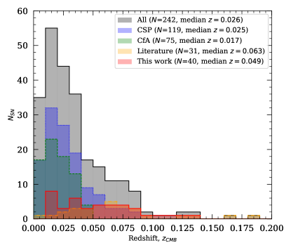
Figure 1: Redshift distribution of the SNe used in the analysis. Note that peculiar SNe Ia are not included here, as well as SNe lacking optical lightcurves. The total number of unique SNe with both optical and NIR lightcurves amounts to 242.

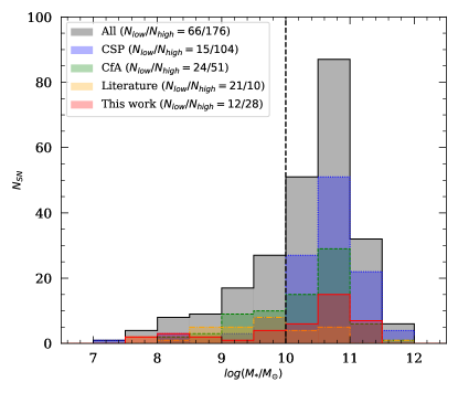
Figure 2: Host galaxy mass distribution of the SNe used in the analysis.

3 Observations

The follow-up observations were obtained with several different facilities, which are described in the following sections. For each instrument used, deep reference images were obtained after the supernova emission had faded away. The reference images were subtracted from the science images in order to facilitate the photometry of the SNe, which can otherwise be affected by the light of the host galaxy. Image subtraction was in most cases performed as part of the reduction pipelines, which all utilize implementation of the convolution algorithms presented in Alard & Lupton (1998).

3.1 Optical data

During the intermediate Palomar Transient Factory (iPTF) survey, the Palomar 48-inch ($P48$) telescope typically delivered $g$ and $R$-band images. The $P48$ image reduction is described by Laher et al. (2014), while the PTF photometric calibration and the photometric system are discussed by Ofek et al. (2012).

Optical follow-up observations were collected using the Palomar 60-inch telescope (P60, $BVgriz$ filters), the 2.56 m Nordic Optical Telescope (NOT) and the Las Cumbres Observatory (LCO) in $UBVRI$ and/or $griz$-bands. The P60 data were reduced using an automated pipeline (Cenko et al., 2006), calibrated against SDSS and the reference images subtracted using FPipe (Fremling et al., 2016). Similarly, the NOT data were reduced with standard IRAF routines using the QUBA pipeline (Valenti et al., 2011), calibrated to the Landolt system through observations of standard stars and SDSS stars in the field. LCOGT data were reduced using lcogtsnpipe (Valenti et al., 2016) by performing PSF-fitting photometry. Zeropoints for images in the $UBVRI$ filters were calculated from Landolt standard fields (Landolt, 1992) taken on the same night by the same telescope. For images in the $griz$ filter set, zeropints were calculated using SDSS magnitudes of stars in the same field as the object.

3.2 Near-IR observations

For 37 out of 42 SNe in our sample, we acquired follow-up observations using the Reionization and Transients InfraRed camera (RATIR). RATIR is a six band simultaneous optical and NIR imager ($riZYJH$-bands) mounted on the autonomous 1.5 m Harold L. Johnson Telescope at the Observatorio Astronómico Nacional on Sierra San Pedro Mártir in Baja California, Mexico (Butler et al., 2012; Watson et al., 2012; Klein et al., 2012; Fox et al., 2012a).

Typical observations include a series of 80-s exposures in the $ri$-bands and 60-s exposures in the $ZYJH$ bands, with dithering between exposures. The fixed IR filters of RATIR cover half of their respective detectors, automatically providing off-target IR sky exposures while the target is observed in the neighbouring filter. Master IR sky frames are created from a median stack of off-target images in each IR filter. No off-target sky frames were obtained on the optical CCDs, but the small galaxy sizes and sufficient dithering allowed for a sky frame to be created from a median stack of selected images in each filter that did not contain either a bright star or extended host galaxy.

Flat-field frames consist of evening sky exposures. Given the lack of a cold shutter in RATIR’s design, IR dark frames are not available. Laboratory testing, however, confirms that the dark current is negligible in both IR detectors (Fox et al., 2012b). Bias subtraction and twilight flat division are performed using algorithms written in python, image alignment is conducted by astrometry.net (Lang et al., 2010) and image co-addition is achieved using swarp (Bertin, 2010). Figure 3 shows a typical set of images, where blue, green and red shows the field-of-view for $i$, $J$ and $H$-band frames, respectively.

For seven SNe Ia in our sample, $J$ and $H$-band observations were also obtained using other facilities, such as HAWK-I on the 8m Very Large Telescope (VLT) (for iPTF14bbr, 14ddi, 14deb, 14eje and 14fww), VIRCAM on the 4m VISTA telescope (iPTF14fpb) and WIRC on the Palomar 200-inch telescope (iPTF14gnl). These observations were processed with the corresponding instrument reduction pipelines.

3.3 Image Subtraction

Image subtraction was performed utilizing the High Order Transform of PSF ANd Template Subtraction (HOTPANTS; Becker, 2015). Point sources were selected across the field-of-view (FOV) to calculate the point-spread function (PSF) in each image, either based on classification from SDSS or through manual inspection. Given the relative paucity of bright point sources in most fields (particularly in the NIR), the PSF was held fixed across the FOV.

The calculated PSFs were utilized to perform PSF-matched photometry on the resulting subtracted images, yielding measurements of the instrumental magnitude of the supernova in each epoch:

$$m_{f,\mathrm{inst}}=-2.5\log_{10}\frac{\rm ADU}{t_{\mathrm{exp}}}$$ (1)

Uncertainties and upper limits were determined by inserting false sources of varying brightness into the RATIR images and repeating the identical process of image subtraction and PSF-matched photometry.

3.4 Photometric Calibration

Photometric calibration of the RATIR data was performed following the process outlined in Ofek et al. (2012). To calculate color and illumination terms, we selected fields with coverage from both SDSS (optical) and UKIDSS (NIR), and obtained photometry for stars (i.e., objects classified as point sources in SDSS) with $r$-band magnitudes between 14 and 18 (with additional flagging for saturation). We measured instrumental magnitudes via PSF-matched photometry for these calibration stars as above.

As a first pass, we calculate a zero-point for each image with no additional corrections (e.g., color and illumination terms). We removed nights with large scatter in the zeropoint (RMS $\geq 0.10$ mag) or individual stars that were clear outliers in the fits (determined via visual inspection).

We then performed a least squares fit using the remaining nights/stars to the following equation for each filter $f$:

$$m_{f} = m_{f,\mathrm{inst}}+ZP+CT_{\mathrm{f,i,j}}\cdot(m_{\mathrm{i}}-m_{\mathrm{j}})+C_{\mathrm{illum}}$$ (2)

where $ZP$ is the zero-point, $CT_{\rm f,i,j}$ is the color term, $m_{\rm i}$ and $m_{\rm j}$ are the filters used for the color correction, and $C_{\rm illum}$ is an illumination correction term accounting for PSF variations depending on the position on the detector.

The color and illumination terms were held fixed for all observations in a given filter, while the zero-point term was allowed to vary freely in each image. The resulting best-fit color terms and zero-point RMS are shown in Table 1. The zero-point RMS is typically $\sim$0.03 mag for the RATIR $r$ to $H$-band.

For fields with SDSS and UKIDSS coverage, calibrated supernova magnitudes were calculated using Equation 2. For fields lacking SDSS coverage, we used photometry from Pan-STARRS1 Data Release 2 (Magnier et al., 2020), which is in a photometric system close to SDSS (Tonry et al., 2012). For fields lacking UKIDSS coverage we used 2MASS (Skrutskie et al., 2006) and the transformation from Hodgkin et al. (2009) to calibrate the $Y$-band RATIR data ($Y=J+0.50\times(J-H)+0.08$).

Table 1: RATIR photometric calibration

Filter	Color term	Color	ZP RMS	Limiting
	$C_{f,ij}$	($i-j$)	[mag]	[mag]
$r$	0.009	($r-i$)	0.031	21.54
$i$	0.030	($r-i$)	0.025	21.52
$z$	-0.048	($i-z$)	0.032	20.80
$Y$	0.046	($Y-J$)	0.031	19.81
$J$	0.057	($J-H$)	0.026	18.94
$H$	-0.054	($J-H$)	0.032	18.27

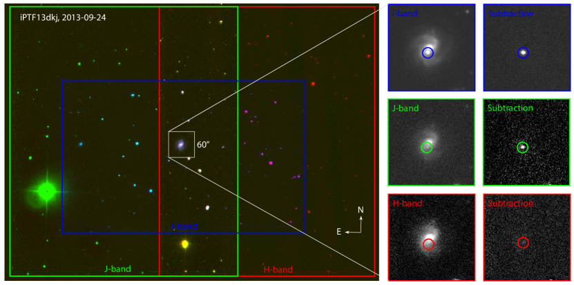
Figure 3: Example of typical RATIR observations for iPTF13dkj (at $z=0.036$) from 2013-09-24. For the RGB composite (left panel), the blue, green and red insets show $i$, $J$ and $H$-band images, respectively. The middle and right panels show the 60″$\times$ 60″region centered on the SN and host galaxy.

4 Analysis

Some of the SNe presented here have previously been published in separate papers:

• Optical and NIR light curves and spectra of iPTF13abc (SN 2013bh) were presented and analysed in Silverman et al. (2013). It is a near identical twin to the peculiar Ia SN 2000cx.

• UV, optical and NIR light curves and spectra of iPTF13asv (SN 2013cv) were presented in Cao et al. (2016) and has additional $H$-band photometry in Weyant et al. (2018). iPTF13asv shows low expansion velocities and persistent carbon absorption features after the maximum, both of which are commonly seen in super-Chandrasekhar events, although its light curve shape and sharp secondary near-IR peak resemble characteristic features of normal SNe Ia.

• Optical light curves and high-resolution spectra of iPTF13dge were presented in Ferretti et al. (2016), and NIR light curves in Weyant et al. (2018). The light curves are compatible with a normal SN Ia with little reddening, and no definite time-variability could be detected in any absorption feature of iPTF13dge.

• UV, optical and NIR observations of iPTF13ebh from the CSP-II collaboration were presented in Hsiao et al. (2015). iPTF13ebh can be categorized as a ”transitional” event, on the fast-declining end of normal SNe Ia, showing NIR spectroscopic properties that are distinct from both the normal and subluminous/91bg-like classes.

• iPTF14atg is a subluminous peculiar SN similar to SN 2002es. It displayed strong, declining ultraviolet emission shortly after explosion. Spectra together with UV, optical and NIR photometry have been extensively analysed in Cao et al. (2015); Kromer et al. (2016).

• UV and optical photometry and spectra of the 1999aa-like SN iPTF14bdn were presented in Smitka et al. (2015).

• iPTF16abc was analyzed by Miller et al. (2018), Ferretti et al. (2017) and Dhawan et al. (2018b). The rapid, near-linear rise, the non-evolving blue colors, and strong absorption from ionized carbon, are interpreted to be the result of either vigorous mixing of radioactive-Ni in the SN ejecta, or ejecta interaction with diffuse material, or a combination of the two.

• iPTF17lf was reddened, spectroscopically normal SN Ia, discovered during a wide-area (2000 deg²) $g$ and $I$-band survey for ”cool transients” as part of a two month extension of iPTF (Adams et al., 2018).

For the other SNe included in our sample (except iPTF14ale, which has no spectroscopic classification), we run the SuperNova IDentification code (SNID Blondin & Tonry, 2007) on the spectra (to be presented in a separate paper). For SNe iPTF13s, iPTF13ddg, iPTF13efe, iPTF14bpz, iPTF14fpb we rely on redshift estimates based on the SN spectral features using SNID. Furthermore, for iPTF13anh, iPTF13asv, iPTF13azs, iPTF13crp and iPTF13dkx, we determine the redshifts from narrow host galaxy lines in the SN spectra.

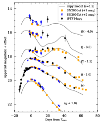
Figure 13: Black symbols show our observed light curves of iPTF14apg. The SNooPy max_model fails to accurately fit the light curves, shown in gray lines (based on the $r$-band stretch, and offset to match the peak magnitudes). In blue and orange are the lightcurves of peculiar Ia SNe 2006bt and 2006, respectively.

For our single spectrum of iPTF14apg, observed 5 days before peak brightness, SNID gives a best match to SN 2004dt at $z=0.088\pm 0.004$, consistent with the spectroscopic redshift of the nearest galaxy. Among the top matches are also SNe 2006ot and 2006bt (Foley et al., 2010), which are peculiar Ia SNe excluded from the Hubble diagram analysis Burns et al. (2018); Uddin et al. (2020). A direct comparison of the light curves of iPTF14apg to those of SNe 2006ot and 2006bt (see Fig. 13) strengthens this classification.

4.1 Host galaxies

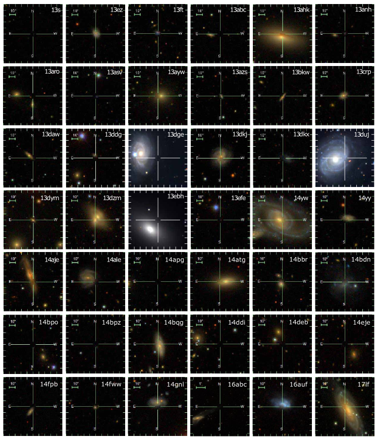
Figure 12: Cutout stamps from SDSS (and PS1) showing the SNe and host galaxies in our sample.

Figure 12 shows cut-out images from the SDSS and PanStarrs surveys, centered on the SN positions. Most SNe can easily be associated with their hosts, while some cases are ambiguous, including:

• iPTF14apg: nearest galaxy is SDSS J123758.69+082301.5 with a spectroscopic redshift $z$=0.08717, separated by 51″, corresponding to a projected distance of 79.4 kpc.

• iPTF14bpo: nearest galaxy is SDSS J171429.74+310905.0 with a spectroscopic redshift $z$=0.07847, separated by 27″, corresponding to a projected distance 38.9 kpc.

• iPTF14ddi: nearest galaxy is SDSS J171036.45+313945.0 with a spectroscopic redshift $z$=0.08133, separated by 40″, corresponding to a projected distance 59.2 kpc.

For the literature sample, we note that SNe PTF10hmv, PTF10nlg and PTF10qyx from Barone-Nugent et al. (2012) have ambiguous hosts.

We estimate the host galaxy stellar mass, $M_{*}$, using the relationship published in Taylor et al. (2011),

$$\log(M_{*}/M_{\odot})=1.15+0.7(m_{g}-m_{i})-0.4M_{i}.$$ (3)

We use $g$ and $i$-band magnitudes from SDSS (or PanStarrs when no SDSS photometry was available), corrected for the Milky Way (MW) extinction. $M_{i}$ is the absolute magnitude in the $i$-band. Table 2 lists the redshifts and coordinates of the SNe in our sample, together with their likely host galaxies and our estimates of the host galaxy stellar mass.

Our mass estimates are consistent with those of (Neill et al., 2009; Chang et al., 2015; Burns et al., 2018), but systematically higher by $\sim$0.2-0.3 dex than the estimates from Ponder et al. (2020) and Uddin et al. (2020), who employ a more sophisticated SED fitting (Fig. 4). However, for consistency when comparing stellar masses between our sample and the CSP, CfA and literature sample, we choose to use our estimates for the combined analysis.

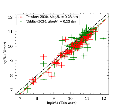
Figure 4: Host galaxy mass estimates from this work, compared to the SNe in common with Ponder et al. (2020) and Uddin et al. (2020).

4.2 Light curve and host galaxy extinction fitting

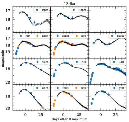
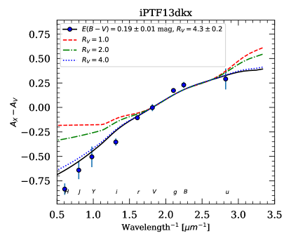
Figure 5: Upper panel shows the max_model fit to iPTF13dkx, a representative SN from our sample at ”moderate” redshift and NIR coverage around peak brightness. Lower panel shows the inferred color excess (normalized with respect to $V-$band) and the best-fit extinction parameters.

We use the SNooPy light curve fitting package developed for the CSP sample (Burns et al., 2011, 2014, 2018) to analyze the light curves the SNe in our sample, including the light curve of the literature sample. To find the time of maximum, $T_{\rm max}$, and color-stretch parameter, $s_{BV}$, and the observed rest-frame peak magnitudes of the SNe, the SNooPy max_model was fitted to the light curves. An example fit is shown in the upper panel of Figure 5 and the derived light curve parameters are given in Tables 3 and 4.

To derive the host galaxy extinction we use the more elaborated color_model. This model allows to fit for the host galaxy extinction taking into account the dependence of SN Ia intrinsic colors on $s_{BV}$ (Burns et al., 2014). It uses parametrized dust extinction laws to calculate the total-to-selective extinction ratio $R_{X}$ in any filter $X$, as a function of $R_{V}$ and $E(B-V)_{\mathrm{host}}$ by the means of synthetic photometry (see Burns et al., 2011). As $R_{V}$ controls the wavelength dependence of the extinction and the host-galaxy color excess $E(B-V)_{\mathrm{host}}$ the amount of the extinction, with observations over a broad range of frequencies it is in principle possible to fit independently for $R_{V}$ and $E(B-V)_{\mathrm{host}}$, which are otherwise correlated. In our analysis we used Cardelli et al. (1989) and O’Donnell (1994) extinction law. For full details on the color_model the reader is referred to Burns et al. (2014, 2018).

We performed two fits for the extinction. First, $R_{V}=2.0$ was assumed for all SN hosts and only $E(B-V)_{\mathrm{host}}$ was fitted. The value $R_{V}=2$ corresponds to our sample average (weighted average $R_{V}=1.9$, $\sigma_{R_{V}}=0.8$) and is close to values commonly found in many SN Ia cosmological analyses, which commonly employ single $R_{V}$. Second, both $E(B-V)_{\textrm{host}}$ and $R_{V}$ were fitted. This is possible because SNe Ia show a small intrinsic color dispersion across optical to NIR bands and the wavelength leverage provided by including NIR observations. Nevertheless, when $E(B-V)_{\mathrm{host}}$ approaches zero (or rather the level of scatter in the intrinsic color, $\sigma_{E(B-V)}\sim 0.06$ mag), the leverage to get meaningful constraints on $R_{V}$ decreases. The results from the second fit are shown in Table 4. Figure 5 lower panel shows an example of the inferred color excess and the best-fit extinction parameters.

It is a long-standing issue that SN analyses have yielded ”unusually” low $R_{V}$ values. This is seen both when minimizing the Hubble residuals using a global $R_{V}$ for cosmological samples and for detailed studies of individual, highly-extinguished SNe (e.g. SNe 2006X and 2014J; Burns et al., 2014; Amanullah et al., 2014). We stress that we only use the observed colors to constrain $E(B-V)_{\mathrm{host}}$ and $R_{V}$, since determining extinction by minimizing Hubble residuals can lead to a bias (Burns et al., 2018; Uddin et al., 2020).

4.3 NIR Hubble diagram

To construct the Hubble diagrams, the distance modulus for filter $X$, $\mu_{X}$, was computed as:

$$\mu_{X}=m_{X}-P_{X}^{N}(s_{BV}-1)-R_{X,BV}E(B-V)_{\mathrm{host}},$$ (4)

where $P_{X}^{N}(s_{BV}-1)$ is the 2-nd order polynomial luminosity-decline-rate relation from Burns et al. (2018) and $R_{X,BV}$ is the total-to-selective absorption coefficient for filter $X$ computed from $R_{V}$ and $E(B-V)_{\mathrm{host}}$. Here, we impose that $R_{V}>0$ and do not correct for dust extinction objects with $E(B-V)_{\mathrm{host}}<0$, i.e. intrinsically blue objects.

Figure 6 shows the resulting $J$ and $H$-band Hubble diagrams for our optical+NIR SNe Ia compilation, including 40 of SNe from our sample presented. iPTF14apg and iPTF14atg, are not included here, as we do not include spectroscopically peculiar SNe Ia (03fg, 06bt, 02es-like nor Iax SNe) in the analysis. Furthermore we apply a set of cuts on the redshift, stretch and color excess distribution on our sample, such that we include only SNe with $z_{CMB}>0.01$, $s_{BV}>0.5$, $E(B-V)_{\rm host}<0.5$ mag, and $E(B-V)_{\rm MW}<0.2$ mag (corresponding to typical sample cuts used in other cosmological analyses, e.g. using SALT2 parameters $-0.3<c<0.3$ and $-3<x_{1}<3$). The solid lines show the best-fit Hubble lines and the dashed lines indicate the scatter expected due to peculiar velocities $v_{\mathrm{pec}}=300$ km/s.

The RMS scatter in the Hubble residuals for the combined sample, after the cuts, is $\sigma_{HR,J}$=0.19 mag (165 SNe) and $\sigma_{HR,H}$=0.21 mag (152 SNe), for $J$ and $H$ respectively. The scatter in $J$ and $H$ does not decrease significantly when using individual best-fit $R_{V}$ instead of a global $R_{V}$.

We note an offset of $0.20\pm 0.05$ mag when comparing the $Y$-band peak magnitudes to the CSP-I sample (also seen when comparing individual $Y$-band light curves of SNe observed simultaneously by RATIR and CSP-II, private communication). We thus add 0.20 mag to the $Y$-band magnitudes listed in Table 3 for the Hubble diagram analysis.

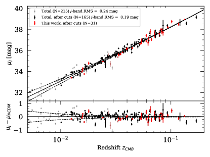
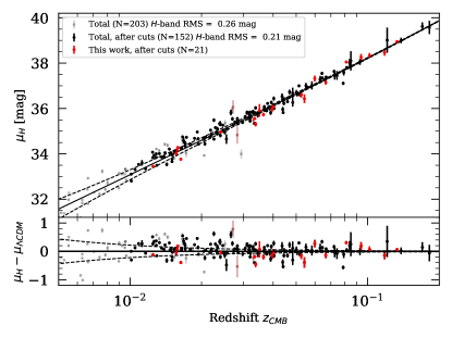
Figure 6: $J$ and $H$-band Hubble diagram and Hubble residuals for the SNe surving our cuts (165 in $J$, 152 in $H$). Red symbols show the SNe presented in this paper, and black symbols the SNe from the literature. Dashed lines indicate the scatter expected due to peculiar velocities $v_{\rm pec}\sim\pm 300$ km s${}^{-1}\hskip 2.84526pt$.

4.4 Correlations with host galaxy stellar mass

Having SN host galaxy stellar masses determined in Sect. 4.1 and color and stretch corrected distances from Sect. 4.3, we can begin to look for correlations.

In Figure 7 we show how our derived color stretch and color excess correlate with host stellar mass. Similar to conclusions reached in previous studies (Sullivan et al., 2011; Childress et al., 2013), we find that low-mass galaxies tend to host SNe with higher stretch ($s_{BV}>0.8$) with moderate extinction ($E(B-V)_{\mathrm{host}}~{}\hbox to0.0pt{$<$\hss}{\lower 4.30554pt\hbox{$\sim$}}0.25$ mag), while high-mass galaxies also host highly reddened SNe and fast-declining SNe.

Following Stanishev et al. (2018) and references therein, we fit the probability density function (PDF) of the computed color excesses for the entire sample, using an exponentially modified Gaussian distribution with a mean $c_{0}$ and standard deviation $\sigma_{c}$ and exponent relaxation parameter $\tau$. We find values $c_{0}$=0.02 mag and $\sigma_{c}$=0.06 mag and $\tau$=0.14. We interpret the Gaussian component as a residual scatter due to intrinsic color variations.

Previous analyses (e.g. Sullivan et al., 2011; Betoule et al., 2014) typically split the sample at $M_{\rm split}=10^{10}$ $M_{\odot}\hskip 2.84526pt$, which seems to be an ”astrophysically reasonable” choice given the fairly distinct difference between the stretch and color excess distributions below and above $\log\,(M_{*}/M_{\odot})$=10.0. Other analyses have chosen a ”statistically motivated” mass split location, either at the median stellar mass ($\log\,(M_{*}/M_{\odot})$$\sim$10.5) of their respective sample or based on some information criterion that maximizes the likelihood (Uddin et al., 2020; Ponder et al., 2020; Thorp et al., 2021). We choose to split our sample at $M_{\mathrm{split}}=10^{10}$ $M_{\odot}\hskip 2.84526pt$, as our fiducial case. Despite adding more SNe in low-mass galaxies from our sub-sample and e.g. the Barone-Nugent et al. (2012) sub-sample, the distribution of host stellar mass for our sample is still skewed towards higher $\log\,(M_{*}/M_{\odot})$. For the combined sample, the median $\log\,(M_{*}/M_{\odot})$=10.50.

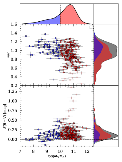
Figure 7: Upper panel: Distribution of stretch versus host galaxy mass. Low-mass galaxies (blue symbols) preferentially host slow-declining ($s>0.8$) SNe, while high-mass galaxies (red symbols) also host fast-declining SNe. Bottom panel: Distribution of fitted $E(B-V)_{\rm host}$ versus host galaxy mass. SNe in low-mass hosts typically have little reddening ($E(B-V)~{}\hbox to0.0pt{$<$\hss}{\lower 4.30554pt\hbox{$\sim$}}0.25$ mag.), while there is a tail of highly extincted SNe occurring in high-mass galaxies.

If we look at the observed distribution of best-fit $R_{V}$ values (Fig. 8), we find a weighted average $R_{V}=2.2$ ($\sigma_{R_{V}}=0.9$) for $\log\,(M_{*}/M_{\odot})$$<10.0$ and $R_{V}=1.7$ ($\sigma_{R_{V}}=0.8$) for $\log\,(M_{*}/M_{\odot})$$>10.0$ host galaxies. The weighted average value of $R_{V}$ for the whole sample is $R_{V}=1.9$ ($\sigma_{R_{V}}=0.9$).

Here, we are not including $R_{V}$ estimates for SNe with color excesses close to the level of intrinsic color scatter $E(B-V)_{\mathrm{host}}<\sigma_{c}\sim 0.06$ mag (where we typically find artificially low $R_{V}$, albeit with large error-bars) nor for highly extinguished SNe $E(B-V)_{\mathrm{host}}>0.5$ mag (which are well fit by $R_{V}$ values ranging from 1.1 to 2.7, but the distribution is likely to be observationally biased towards finding SNe with low $R_{V}$).

In order to test the hypothesis that the distributions of $R_{V}$ in the low and high stellar mass bins are statistically compatible from being drawn from the same underlying distribution we perform a Kolmogorov-Smirnov (K-S) test. The K-S test yields a $p$-value of only 0.015, hence suggesting that the distributions are significantly different, with more than 95% confidence level.

Even though the weighted mean values are statistically consistent with the global mean $R_{V}$ value, we stress that the wide, non-gaussian, probability distributions are different.

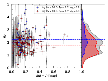
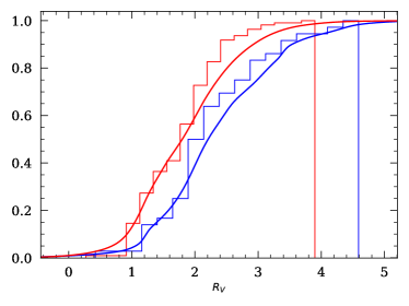
Figure 8: Left panel shows the distribution of best-fit $R_{V}$ and $E(B-V)_{\mathrm{host}}$ for the SNe included in the analysis. The color indicates if the SN occurred in a low- (blue) or high-mass host (red). The middle panel shows the coadded probability distribution of the best-fit $R_{V}$ values. The right panel shows the cumulative $R_{V}$ distribution for the low- and high-mass galaxies in blue and red, respectively.

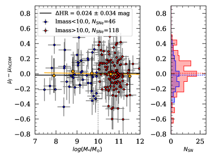
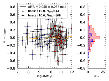
Figure 9: $J$ and $H$-band Hubble residuals versus host galaxy stellar mass from fitting optical and NIR lightcurves with the color_model (each SN corrected with best-fit $E(B-V)_{\mathrm{host}}$ and $R_{V}$). Orange symbols show the binned mean and standard deviation of the Hubble residuals in five mass bins, while the orange line is the fitted slope ($-0.01\pm 0.02$ mag/dex in $J$, $0.0\pm 0.02$ mag/dex in $H$).

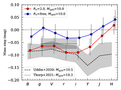
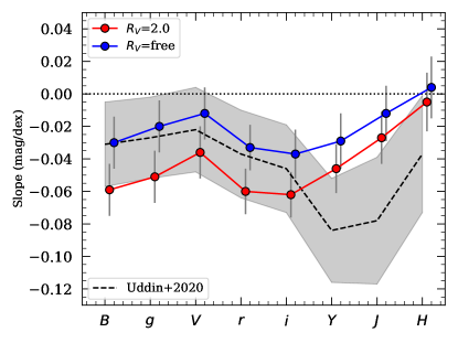
Figure 10: Size of the mass-step (left panel) or mass-slope (right panel) in different filters ($BgVriYJH$). Blue symbols show the resulting mass-steps/slopes if we use the best-fit $R_{V}$ for each individual SN, and red symbols if we use a global $R_{V}=2.0$. Gray dashed lines show the mass-steps from Uddin et al. (2020) and (their Table 2) for the same cuts on $E(B-V)_{\mathrm{host}}<0.5$ mag and $s_{BV}>0.5$, but for $\log M_{\rm split}=10.5$ and including SNe at $z<0.01$. The dotted line shows the mass-step in Thorp et al. (2021).

For the low- and high-mass bins, we compute a weighted mean and standard deviation of the Hubble residuals for $BVgriYJH$ filters (horizontal black lines in Fig. 9 and 11). For each filter $X$, we will refer to any Hubble residual offset between the two bins as a ”mass-step”, $\Delta_{HR}(X)$. To further investigate the behaviour of the Hubble residuals, we divide the sample into five mass bins (orange symbols in Fig. 9), to see if there are any additional effects towards the edges of the host mass distribution. Following Uddin et al. (2020), we also fit a slope to the Hubble residuals as a function of host mass (yellow lines in Fig. 9 and 11) using Orthogonal Distance Regression (ODR).

We find that using a global value $R_{V}=2.0$ (close to the average $R_{V}$ for the entire sample) for all SNe in low- and high-mass host galaxies, we reproduce a significant ($\sim 2\sigma$) mass-step in optical $BVgri$-band Hubble residuals $\Delta_{HR}\sim-0.07\pm 0.03$ mag, while for NIR $JH$-bands there is no significant mass step ($\Delta_{HR}(J)=-0.021\pm 0.033$ mag and $\Delta_{HR}(H)=0.020\pm 0.036$ mag), shown as red symbols in Fig. 10 (left panel). A similar trend is seen when fitting a slope to the Hubble residuals as a function of host mass. For optical $BVgri$-bands we find a slopes of $\sim 0.06\pm 0.02$ mag/dex, while in the NIR the slopes are smaller ($-0.027\pm 0.016$ mag/dex and $-0.005\pm 0.018$ mag/dex in $J$ and $H$, respectively) shown as red symbols in right panel of Fig. 10.

When correcting each SN individually by their best-fit $R_{V}\times E(B-V)_{host}$ we see no significant mass-step or mass-slope in the Hubble residuals, across the optical and NIR bands (blue symbols in Fig. 10).

This result seems valid when changing the cuts on $z$, $s_{BV}$ and $E(B-V)_{\mathrm{host}}$, and perhaps more importantly the choice of $M_{\mathrm{split}}$. Choosing $M_{\rm split}=10^{10.5}$ $M_{\odot}\hskip 2.84526pt$(the median stellar host galaxy mass of our SNe compilation), we do see a (non-significant) mass-step across optical and NIR $\Delta_{HR}\sim-0.04\pm 0.03$ mag. We find that our results are in line with with Brout & Scolnic (2021), who modelled host galaxy reddening as separate Gaussian distributions for galaxies below and above $\log\,(M_{*}/M_{\odot})$=10. They found that SNe in low-mass hosts, the average $\langle R_{V}\rangle=2.75\pm 0.35$, whereas for SNe in high-mass hosts, $\langle R_{V}\rangle=1.5\pm 0.25$, with both sub-samples having a wide distributions $\sigma_{R_{V}}=1.3$. This is in fair agreement with Salim et al. (2018), who find that on average, dusty, high-mass quiescent galaxies have lower $R_{V}$ values ($\langle{R_{V}}\rangle=2.61$), whereas low-mass star forming galaxies tend to have higher values for $R_{V}$ ($\langle{R_{V}}\rangle=3.15$).

Uddin et al. (2020) found nominal evidence for a consistent mass-step in both the optical and NIR using the CSP-I sample ($\Delta_{HR,J}=-0.103\pm 0.050$ mag, and $\Delta_{HR,H}=-0.097\pm 0.047$ mag) using similar cuts on the sample, although including SNe with $z<0.01$ and having the mass-step located at $\log\,(M_{*}/M_{\odot})$=10.5 (shown as gray dashed lines in Fig. 10). We can not fully reproduce the NIR mass-step reported by Uddin et al. (2020), even if we use their host masses and the same best-fit extinction. We note that they do use updated Phillips-relations, correcting for stretch using more flexible spline functions calibrated using unpublished data from CSP-II (C. Burns and S. Uddin, private communication), but we do not expect this to be result in the observed differences in our plots.

Ponder et al. (2020) also report a $H$-band mass-step $\Delta_{HR,H}=-0.18\pm 0.05$ mag (mass-step located at $\log\,(M_{*}/M_{\odot})$=10.44) using a compilation of 99 SNe from the literature. However, after removing two outliers, the step reduces to $\Delta_{HR,H}=-0.10\pm 0.04$ mag. It is unclear if their results are due to the lack of NIR stretch corrections and/or color-corrections.

Recently, Thorp et al. (2021) analyzed optical ($griz$) lightcurves of 157 nearby SNe Ia (0.015 $<z<$ 0.08) from the Foundation DR1 dataset using the BayesSN lightcurve fitter (Mandel et al., 2011, 2020). When splitting their sample at $\log\,(M_{*}/M_{\odot})$=10, they find $R_{V}=2.84\pm 0.31$ in low-mass hosts, and $R_{V}=2.58\pm 0.23$ in high-mass hosts. They conclude that these values are consistent with the global value of $R_{V}=2.61\pm 0.21$, estimated for the full sample, and can not be an explanation of the mass step. After corrections, their resulting mass-step is $\Delta_{HR}=0.050\pm 0.022$ mag (shown as gray dotted line in left panel of Fig. 10).

5 Discussion

The relation between SN Ia luminosity and host galaxy properties is of great interest for SN Ia progenitor studies as well as for cosmology, as a third empirical correction (Sullivan et al., 2010; Lampeitl et al., 2010; Kelly et al., 2010). While the correlation has been seen nearly ubiquitously across different samples (see e.g. Brout et al., 2019; Smith et al., 2020), there is a significant debate about the physical origin of this relation. There has been speculation that the mass-step may be driven by the age of the stellar population, metallicity or star formation rate (Sullivan et al., 2010; Gupta et al., 2011; D’Andrea et al., 2011; Hayden et al., 2013; Childress et al., 2014; Rigault et al., 2020; Rose et al., 2020). However, it is possible that this correlation arises due to different SN Ia environments in different host galaxy types.

While most studies pertaining to SN luminosity and host galaxy correlations in the optical, recently there have been reports of the possible detection of the mass-step in the NIR wavebands (Ponder et al., 2020; Uddin et al., 2020). In this study, we exploit the multi-wavelength, well-sampled lightcurves of the SNe in our sample and compute the mass-step/slope after stretch and color corrections, fitting the $R_{V}$ parameter individually for each SN. We find that when fitting the $R_{V}$ value for each SN, we see a mass step consistent with zero in all filters from $B$ to $H-$band (see Figure 10). However, when fixing the $R_{V}$ value to the sample average, as is done in previous studies, we find that there is a mass step of $\sim$ 0.07 - 0.1 mag in the optical ($BVgri$) while no significant step is seen in the NIR ($YJH$).

Since the free $R_{V}$ case yields mass steps that are consistent with zero, it is likely that the origin of the mass step is due to variations of dust properties in the interstellar medium of the host galaxies. However, more detailed studies would be required to rule out intrinsic effects. In fact, there are indications that there are two SN populations, having different SN ejecta velocities and different intrinsic colors, which also trace the host galaxy stellar mass (see e.g. Polin et al., 2019; Siebert et al., 2020; Pan, 2020). Childress et al. (2013) and Gonzalez-Gaitan et al. (2020) simulate the effect of having separate color-luminosity corrections for low- and high-mass galaxies. They find that multiple free color-luminosity slope parameters may explain away the mass-step, suggesting that the origin of mass-step is a difference in intrinsic color-luminosity relation ($\beta_{int}c_{int}$) of two SN populations found in galaxies with different masses as opposed to different dust properties.

6 Conclusion

Many studies in the literature have suggested the need for an additional standardization parameter for SNe Ia, beyond the lightcurve shape and color. In particular, firm evidence has been put forward for a correlation between residuals in the Hubble diagram at optical wavelengths, and the host galaxy stellar mass (Sullivan et al., 2010; Lampeitl et al., 2010; Kelly et al., 2010; Gupta et al., 2011; D’Andrea et al., 2011; Hayden et al., 2013; Childress et al., 2014; Rose et al., 2020). The underlying cause of these correlations is not completely understood, with some suggestions that this could be due to correlation with age/metallicity of the underlying stellar population, however, there is also evidence pointing to this correlation arising from differences in dust properties of the SN hosts.

Our work differs from previous studies in that we use a sample of SNe Ia, found in the untargeted PTF/iPTF surveys, which adds a significant number of low-mass host galaxies. Furthermore, our data-set includes multi-wavelength follow-up observations, including near-IR, which allows us to infer the total-to-selective extinction parameter, $R_{V}$, for each SN individually. This is motivated by the findings in e.g. Amanullah et al. (2015) and Burns et al. (2018), suggesting that the wavelength dependence of dimming by host galaxy mass varies between SNe, making the use of a single value of $R_{V}$ questionable. Using a parameterized extinction relation by CCM, we fit for both the color-excess, $E(B-V)$, and $R_{V}$ using SNooPy color_model fits of the multi-band data. In other words, our estimate of the extinction along the line-of-sight of each SN is not derived from the Hubble residuals. When examining the Hubble residuals, we do not find a significant correlation with stellar mass at optical or NIR wavelengths.

If we, instead, assume a single value for $R_{V}$ to correct all SNe fitting only the color excess, we recover the ”mass-step” in optical filters. In the NIR, we find no significant dependence on the stellar mass, independently of how $R_{V}$ is measured, i.e., individually or globally. This is consistent with the interpretation made by (Brout & Scolnic, 2021), that the mass-step is likely caused by differences in dust properties of the low- and high-mass SN host galaxies.

7 Acknowledgements

We are grateful for valuable comments from Jakob Nordin and feedback from the CSP team (Chris Burns, Eric Hsiao, Mark Phillips and Shuvo Uddin). We thank M. L. Graham for helping to obtain follow-up observations with Las Cumbres Observatory in 2013.

A.G acknowledges support from the Swedish Research Council under Dnr VR 2016-03274 and 2020-03444. T.P. acknowledges the financial support from the Slovenian Research Agency (grants I0-0033, P1-0031, J1-8136 and Z1-1853). Research by S.V. is supported by NSF grants AST-1813176 and AST-2008108.

This work makes use of observations from the Las Cumbres Observatory network. The LCO team was supported by NSF grants AST-1313484 and AST-1911225. The intermediate Palomar Transient Factory project is a scientific collaboration among the California Institute of Technology, Los Alamos National Laboratory, the University of Wisconsin, Milwaukee, the Oskar Klein Center, the Weizmann Institute of Science, the TANGO Program of the University System of Taiwan, and the Kavli Institute for the Physics and Mathematics of the Universe. LANL participation in iPTF is supported by the US Department of Energy as a part of the Laboratory Directed Research and Development program

Table 2: 42 SNe Ia from the iPTF survey and their associated host galaxies.

SN	$z_{\rm helio.}$	$z_{\rm CMB}$	R.A.	Decl.	Host galaxy	$\log\left(\frac{M_{*}}{M_{\odot}}\right)$
iPTF13S	0.059a	0.060	203.222074	+35.959372	SDSS J133253.27+355733.4	7.97
iPTF13ez	0.04363	0.04470	182.463737	+19.787693	KUG 1207+200	10.19
iPTF13ft	0.03884	0.03963	199.947067	+33.024961	SDSS J131947.32+330131.8	8.80
iPTF13abc (SN 2013bh)	0.07436	0.07498	225.554527	+10.645905	SDSS J150214.17+103843.6	10.33
iPTF13ahk	0.02639	0.02712	203.805002	+34.678903	NGC 5233	11.27
iPTF13anh	0.0615b	0.0625	196.710215	+15.575657	SDSS J130650.44+153432.7	8.51
iPTF13aro	0.08462	0.08497	236.884308	+23.023956	SDSS J154732.26+230111.8	10.75
iPTF13asv (SN 2013cv)	0.0362b	0.0364	245.679971	+18.959717	SDSS J162243.02+185733.8	7.71
iPTF13ayw	0.05385	0.05418	234.889650	+32.093954	SDSS J153933.08+320538.3	11.15
iPTF13azs (SN 2013cx)	0.0338b	0.03376	256.067046	+41.510353	SDSS J170415.96+413036.8	9.79
iPTF13bkw	0.06393	0.06491	200.489840	+11.735753	SDSS J132157.57+114406.2	10.56
iPTF13crp	0.0630b	0.0621	29.750591	+16.264187	SDSS J015900.28+161551.5	10.71
iPTF13daw	0.07755	0.07680	40.880381	+1.984422	SDSS J024331.69+015908.4	10.82
iPTF13ddg	0.084a	0.083	11.961798	+31.821517	SDSS J004750.94+314922.5	9.71
iPTF13dge	0.015854	0.015805	75.896169	+1.571493	NGC 1762	10.87
iPTF13dkj	0.03623	0.03503	347.211539	+20.069088	CGCG 454-001	10.50
iPTF13dkx	0.0345b	0.0335	20.221425	+3.339925	SDSS J012052.56+032023.0	9.13
iPTF13duj (SN 2013fw)	0.016952	0.015879	318.436571	+13.575875	NGC 7042	10.99
iPTF13dym	0.04213	0.04091	351.125804	+14.651100	SDSS J232430.20+143903.5	9.93
iPTF13dzm	0.018193	0.017219	17.824325	+33.112441	NGC 0414	10.25
iPTF13ebh	0.013269	0.012493	35.499900	+33.270479	NGC 890	11.23
iPTF13efe	0.070a	0.071	130.913761	+16.177023	SDSS J084339.26+161037.5	8.39
iPTF14yw (SN 2014aa)	0.016882	0.017972	176.264696	+19.973620	NGC 3861	10.86
iPTF14yy	0.04311	0.04423	186.538205	+9.978942	SDSS J122608.78+095847.1	10.40
iPTF14aje	0.02769	0.02825	231.300298	-1.814299	UGC 9839	10.96
iPTF14ale	0.093226	0.093835	219.587725	+27.334341	SDSS J143822.02+272010.6	11.36
iPTF14apg	0.08717	0.088278	189.480312	+8.384737	SDSS J123758.69+082301.5 (?)	11.01
iPTF14atg	0.02129	0.02222	193.186849	+26.470284	IC 0831	10.88
iPTF14bbr	0.06549	0.06662	186.546284	+7.668036	SDSS J122611.21+074000.9	10.85
iPTF14bdn	0.01558	0.016348	202.687002	+32.761788	UGC 8503	8.37
iPTF14bpo	0.07847	0.07838	258.629576	+31.157130	SDSS J171429.74+310905.0 (?)	10.77
iPTF14bpz	0.120a	0.120	234.215837	+21.767070	SDSS J153651.66+214556.5	8.48
iPTF14bqg	0.03291	0.03303	245.986385	+36.228411	SDSS J162356.48+361339.3	10.84
iPTF14ddi	0.08133	0.08126	257.639496	+31.659566	SDSS J171036.45+313945.0 (?)	11.16
iPTF14deb	0.13243	0.13293	229.614857	+19.742951	SDSS J151828.02+194455.3	11.42
iPTF14eje	0.11888	0.11774	348.293114	+29.191366	SDSS J231309.15+291111.6	11.38
iPTF14fpb	0.061a	0.060	11.944065	+11.240145	SDSS J004746.83+111415.9	10.14
iPTF14fww	0.10296	0.10183	10.326226	+15.438180	SDSS J004118.33+152616.2	10.07
iPTF14gnl	0.053727	0.052572	5.951363	-3.857740	SDSS J002348.33-035120.6	10.59
iPTF16abc (SN 2016bln)	0.023196	0.024128	203.689542	+13.853974	NGC 5221	10.85
iPTF16auf (SN 2016ccz)	0.01499	0.01563	217.788598	+27.236051	MRK 0685	9.53
iPTF17lf (SN 2017lf)	0.01464	0.01407	48.139952	+39.320608	NGC 1233	10.50
$(a):$ Redshift determined using SNID. $(b):$ Redshift determined from host galaxy lines in the SN spectra.

Table 3: Fitted light curve peak magnitudes, $k$-corrected to restframe and corrected for MW extinction using the SNooPy max_model.

SN	$B_{max}$	$V_{max}$	$u_{max}$	$g_{max}$	$r_{max}$	$i_{max}$	$Y_{max}$	$J_{max}$	$H_{max}$
iPTF13s	–	–	–	17.47 (0.01)	17.75 (0.01)	18.40 (0.06)	18.58 (0.07)	18.22 (0.11)	–
iPTF13ez	–	–	–	–	17.43 (0.01)	17.80 (0.06)	17.62 (0.06)	17.72 (0.08)	–
iPTF13ft	–	–	–	–	16.84 (0.01)	17.50 (0.02)	17.66 (0.05)	17.46 (0.08)	17.58 (0.13)
iPTF13abc	18.29 (0.12)	18.32 (0.09)	–	18.28 (0.06)	18.27 (0.03)	19.03 (0.05)	19.04 (0.11)	–	–
iPTF13ahk	21.02 (0.42)	19.53 (0.39)	–	20.24 (0.13)	18.66 (0.02)	18.46 (0.10)	17.67 (0.14)	17.18 (0.28)	17.91 (0.30)
iPTF13anh	18.11 (0.03)	17.97 (0.03)	18.68 (0.05)	–	18.19 (0.01)	18.64 (0.01)	18.69 (0.05)	18.58 (0.22)	–
iPTF13aro	19.04 (0.05)	18.96 (0.04)	19.35 (0.12)	18.93 (0.06)	19.05 (0.02)	19.47 (0.03)	19.38 (0.14)	19.24 (0.31)	–
iPTF13asv	16.32 (0.02)	16.37 (0.02)	16.39 (0.04)	16.28 (0.02)	16.52 (0.01)	17.23 (0.02)	17.50 (0.04)	17.15 (0.04)	17.32 (0.08)
iPTF13ayw	18.20 (0.04)	18.18 (0.05)	–	18.19 (0.03)	18.01 (0.01)	18.50 (0.01)	18.37 (0.06)	18.44 (0.26)	18.14 (0.19)
iPTF13azs	17.93 (0.04)	17.58 (0.04)	18.52 (0.06)	17.75 (0.05)	17.60 (0.01)	17.90 (0.01)	17.66 (0.04)	17.31 (0.05)	17.13 (0.08)
iPTF13bkw	18.39 (0.03)	18.25 (0.03)	18.66 (0.07)	18.43 (0.02)	18.29 (0.01)	18.83 (0.06)	18.98 (0.15)	19.16 (0.26)	–
iPTF13crp	18.86 (0.02)	18.40 (0.02)	19.21 (0.06)	18.70 (0.05)	18.38 (0.01)	18.82 (0.02)	18.71 (0.28)	18.26 (0.27)	–
iPTF13daw	19.20 (0.02)	–	–	19.12 (0.02)	19.08 (0.01)	19.49 (0.03)	19.14 (0.26)	–	–
iPTF13ddg	18.79 (0.02)	–	–	18.78 (0.01)	18.80 (0.01)	19.36 (0.01)	19.22 (0.07)	19.29 (0.26)	–
iPTF13dge	15.13 (0.01)	15.19 (0.01)	15.64 (0.03)	15.28 (0.00)	15.28 (0.01)	15.86 (0.01)	15.80 (0.04)	15.61 (0.08)	15.81 (0.08)
iPTF13dkj	17.06 (0.01)	–	–	16.97 (0.01)	17.03 (0.01)	17.53 (0.01)	17.33 (0.05)	17.18 (0.11)	17.59 (0.28)
iPTF13dkx	17.22 (0.01)	17.04 (0.02)	17.52 (0.04)	17.12 (0.01)	17.11 (0.01)	17.53 (0.01)	17.52 (0.07)	17.19 (0.06)	17.31 (0.05)
iPTF13duj	15.11 (0.01)	15.07 (0.01)	15.51 (0.06)	–	15.09 (0.02)	15.71 (0.02)	15.85 (0.04)	15.69 (0.05)	15.89 (0.05)
iPTF13dym	17.75 (0.02)	–	–	17.50 (0.02)	17.49 (0.02)	17.86 (0.05)	17.82 (0.09)	17.78 (0.09)	17.83 (0.14)
iPTF13dzm	15.81 (0.02)	–	–	15.59 (0.02)	15.54 (0.01)	15.94 (0.03)	–	–	–
iPTF13ebh	15.08 (0.01)	14.93 (0.01)	15.75 (0.01)	14.95 (0.01)	14.91 (0.01)	15.32 (0.01)	15.27 (0.04)	15.01 (0.03)	15.20 (0.05)
iPTF13efe	18.32 (0.02)	–	–	18.28 (0.02)	18.34 (0.02)	18.99 (0.02)	19.13 (0.09)	18.88 (0.33)	–
iPTF14yw	–	–	–	16.08 (0.05)	15.85 (0.02)	16.43 (0.03)	16.43 (0.12)	16.28 (0.14)	–
iPTF14yy	18.43 (0.03)	18.12 (0.05)	–	–	18.12 (0.01)	18.50 (0.01)	18.25 (0.03)	–	–
iPTF14aje	18.88 (0.06)	18.05 (0.03)	19.67 (0.03)	18.71 (0.02)	17.73 (0.01)	17.75 (0.02)	17.33 (0.08)	16.76 (0.26)	16.85 (0.38)
iPTF14ale	–	–	19.33 (0.02)	19.29 (0.01)	19.77 (0.02)	19.50 (0.05)	19.59 (0.13)	19.89 (0.14)
iPTF14bbr	–	–	18.10 (0.05)	18.25 (0.03)	18.75 (0.08)	18.79 (0.36)	18.48 (0.14)	18.79 (0.10)
iPTF14bdn	14.78 (0.03)	15.04 (0.03)	14.87 (0.04)	14.92 (0.01)	15.45 (0.01)	15.56 (0.04)	15.20 (0.03)	15.42 (0.05)
iPTF14bpo	18.95 (0.07)	–	–	18.93 (0.04)	18.98 (0.03)	19.43 (0.07)	19.21 (0.10)	19.09 (0.27)	–
iPTF14bpz	19.83 (0.02)	–	–	19.75 (0.01)	19.79 (0.03)	20.43 (0.07)	20.74 (0.29)	–	–
iPTF14bqg	18.91 (0.05)	18.30 (0.05)	–	18.70 (0.11)	17.88 (0.02)	18.07 (0.02)	17.67 (0.07)	16.99 (0.08)	17.23 (0.14)
iPTF14ddi	19.01 (0.04)	–	–	18.90 (0.02)	18.95 (0.01)	19.50 (0.02)	–	19.47 (0.05)	19.68 (0.05)
iPTF14deb	21.00 (0.06)	20.77 (0.04)	–	-99.90 (-99.00)	20.57 (0.03)	–	–	20.60 (0.06)	20.73 (0.06)
iPTF14eje	19.42 (0.01)	–	–	19.32 (0.04)	19.54 (0.02)	20.08 (0.08)	–	19.92 (0.15)	20.10 (0.14)
iPTF14fpb	18.14 (0.01)	–	–	18.02 (0.00)	18.11 (0.01)	18.78 (0.02)	–	18.78 (0.16)	18.93 (0.13)
iPTF14fww	–	–	–	19.40 (0.01)	19.52 (0.06)	20.06 (0.09)	–	20.08 (0.15)	19.97 (0.11)
iPTF14gnl	17.52 (0.04)	17.58 (0.05)	–	17.53 (0.01)	17.68 (0.02)	18.02 (0.05)	–	18.07 (0.09)	18.23 (0.13)
iPTF16abc	15.95 (0.04)	15.93 (0.05)	16.07 (0.04)	15.81 (0.01)	15.93 (0.01)	16.49 (0.01)	16.67 (0.03)	16.36 (0.03)	16.60 (0.04)
iPTF16auf	15.46 (0.02)	15.47 (0.01)	16.24 (0.12)	15.32 (0.01)	15.33 (0.01)	15.70 (0.01)	15.87 (0.05)	15.48 (0.07)	15.73 (0.08)
iPTF17lf	–	–	–	18.79 (0.06)	17.27 (0.06)	17.04 (0.03)	16.73 (0.11)	–	–

Table 4: Light curve parameters for the supernovae using the SNooPy color_model.

SN	$T_{\rm max}$	$s_{BV}$	$E(B-V)_{\rm MW}$	$E(B-V)_{\rm host}$	$R_{V}$
iPTF13s	56338.13 (0.19)	1.091 (0.027)	0.011	-0.011 (0.013)	2.0 (-)
iPTF13ez	56346.87 (0.07)	0.879 (0.020)	0.043	0.309 (0.052)	1.4 (0.2)
iPTF13ft	56356.87 (0.18)	1.089 (0.015)	0.015	-0.049 (0.028)	2.0 (-)
iPTF13abc	56385.78 (1.09)	0.850 (0.029)	0.030	0.018 (0.026)	2.0 (-)
iPTF13ahk	56396.20 (0.36)	0.508 (0.043)	0.013	1.980 (0.057)	1.1 (0.2)
iPTF13anh	56414.59 (0.09)	0.945 (0.006)	0.022	0.161 (0.015)	2.3 (0.4)
iPTF13aro	56423.93 (0.20)	0.875 (0.027)	0.044	0.186 (0.019)	2.0 (0.2)
iPTF13asv	56429.54 (0.16)	1.098 (0.018)	0.044	-0.030 (0.011)	2.4 (1.2)
iPTF13ayw	56431.17 (0.14)	0.756 (0.021)	0.029	0.210 (0.017)	2.0 (0.3)
iPTF13azs	56436.78 (0.15)	1.035 (0.019)	0.019	0.466 (0.013)	3.2 (0.2)
iPTF13bkw	56459.11 (0.08)	1.014 (0.016)	0.022	0.282 (0.019)	1.0 (0.1)
iPTF13crp	56527.92 (0.21)	1.262 (0.016)	0.050	0.407 (0.020)	2.5 (0.5)
iPTF13daw	56543.15 (0.56)	0.718 (0.011)	0.034	0.138 (0.021)	3.9 (0.3)
iPTF13ddg	56547.89 (0.09)	1.014 (0.010)	0.060	0.143 (0.013)	2.5 (0.1)
iPTF13dge	56556.36 (0.02)	1.023 (0.004)	0.078	0.143 (0.007)	2.4 (0.4)
iPTF13dkj	56560.45 (0.06)	0.929 (0.011)	0.147	0.167 (0.006)	2.5 (0.5)
iPTF13dkx	56565.52 (0.10)	1.202 (0.011)	0.027	0.188 (0.008)	4.3 (0.2)
iPTF13duj	56601.58 (0.11)	1.099 (0.017)	0.067	0.150 (0.012)	1.4 (0.2)
iPTF13dym	56610.27 (0.68)	0.541 (0.042)	0.038	0.021 (0.012)	1.9 (1.5)
iPTF13dzm	56614.32 (0.08)	0.675 (0.014)	0.049	0.205 (0.020)	1.6 (0.1)
iPTF13ebh	56623.24 (0.03)	0.609 (0.005)	0.067	0.069 (0.007)	3.1 (1.0)
iPTF13efe	56641.44 (0.27)	1.193 (0.023)	0.021	0.100 (0.010)	1.7 (0.1)
iPTF14yw	56729.58 (0.16)	0.848 (0.029)	0.026	0.276 (0.019)	1.3 (0.4)
iPTF14yy	56733.27 (0.15)	0.802 (0.020)	0.020	0.305 (0.018)	3.2 (0.2)
iPTF14aje	56758.24 (0.10)	0.650 (0.015)	0.152	0.794 (0.018)	2.5 (0.1)
iPTF14ale	56771.54 (0.26)	0.989 (0.025)	0.015	0.289 (0.019)	1.3 (0.3)
iPTF14bbr	56804.28 (0.91)	1.028 (0.054)	0.021	0.122 (0.009)	2.4 (0.2)
iPTF14bdn	56822.23 (0.09)	1.115 (0.012)	0.010	0.100 (0.006)	3.5 (0.3)
iPTF14bpo	56830.32 (0.67)	0.757 (0.026)	0.034	0.066 (0.029)	2.0 (0.1)
iPTF14bpz	56836.01 (0.22)	1.198 (0.022)	0.046	0.090 (0.018)	2.0 (0.3)
iPTF14bqg	56837.98 (0.25)	0.910 (0.050)	0.013	1.076 (0.035)	1.4 (0.3)
iPTF14ddi	56850.63 (0.10)	0.858 (0.016)	0.032	0.099 (0.023)	1.2 (0.1)
iPTF14deb	56841.45 (0.30)	0.613 (0.034)	0.039	0.222 (0.021)	2.2 (0.4)
iPTF14eje	56901.79 (0.66)	1.084 (0.040)	0.108	0.080 (0.016)	3.0 (1.0)
iPTF14fpb	56928.80 (0.53)	1.086 (0.017)	0.072	0.133 (0.017)	1.5 (0.1)
iPTF14fww	56929.64 (0.64)	1.229 (0.035)	0.063	0.081 (0.012)	3.0 (0.2)
iPTF14gnl	56957.26 (0.11)	0.953 (0.017)	0.027	0.083 (0.025)	1.8 (0.6)
iPTF16abc	57499.01 (0.08)	1.070 (0.010)	0.024	0.105 (0.005)	2.4 (0.2)
iPTF16auf	57537.80 (0.09)	1.189 (0.012)	0.013	0.248 (0.021)	2.9 (0.3)
iPTF17lf	57776.60 (0.95)	0.946 (0.032)	0.134	2.129 (0.088)	1.2 (0.1)

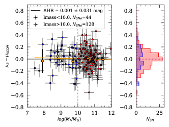
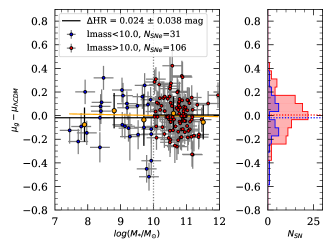
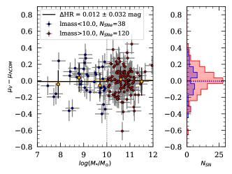
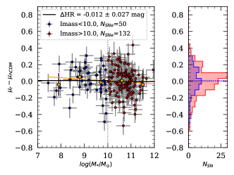
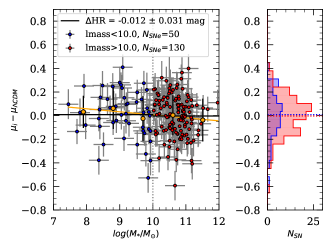
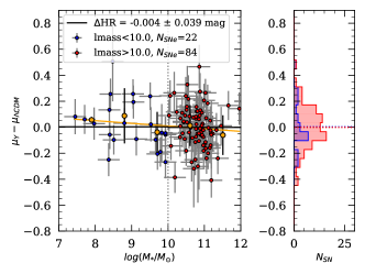
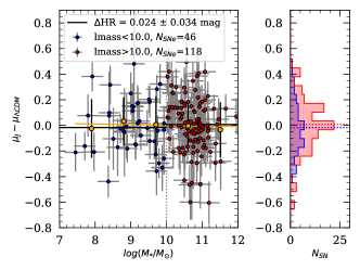
Figure 11: Hubble residuals versus host galaxy stellar mass from fitting from optical ($BgVri$) and NIR ($YJH$) lightcurves with the SNooPy color_model (i.e. each SN corrected with best-fit $E(B-V)_{\mathrm{host}}$ and $R_{V}$). Orange symbols show the binned mean and standard deviation of the Hubble residuals in five mass bins, while the orange line is the fitted slope.

References

- Adams et al. (2018) Adams, S. M., Blagorodnova, N., Kasliwal, M. M., et al. 2018, PASP, 130, 034202, doi: 10.1088/1538-3873/aaa356
- Alard & Lupton (1998) Alard, C., & Lupton, R. H. 1998, ApJ, 503, 325, doi: 10.1086/305984
- Amanullah et al. (2014) Amanullah, R., Goobar, A., Johansson, J., et al. 2014, ApJ, 788, L21, doi: 10.1088/2041-8205/788/2/L21
- Amanullah et al. (2015) Amanullah, R., Johansson, J., Goobar, A., et al. 2015, MNRAS, 453, 3300, doi: 10.1093/mnras/stv1505
- Avelino et al. (2019) Avelino, A., Friedman, A. S., Mandel, K. S., et al. 2019, ApJ, 887, 106, doi: 10.3847/1538-4357/ab2a16
- Barone-Nugent et al. (2012) Barone-Nugent, R. L., Lidman, C., Wyithe, J. S. B., et al. 2012, MNRAS, 425, 1007, doi: 10.1111/j.1365-2966.2012.21412.x
- Becker (2015) Becker, A. 2015, HOTPANTS: High Order Transform of PSF ANd Template Subtraction, Astrophysics Source Code Library. http://ascl.net/1504.004
- Bertin (2010) Bertin, E. 2010, SWarp: Resampling and Co-adding FITS Images Together. http://ascl.net/1010.068
- Betoule et al. (2014) Betoule, M., Kessler, R., Guy, J., et al. 2014, A&A, 568, A22, doi: 10.1051/0004-6361/201423413
- Blondin et al. (2015) Blondin, S., Dessart, L., & Hillier, D. J. 2015, MNRAS, 448, 2766, doi: 10.1093/mnras/stv188
- Blondin & Tonry (2007) Blondin, S., & Tonry, J. L. 2007, ApJ, 666, 1024, doi: 10.1086/520494
- Brout & Scolnic (2021) Brout, D., & Scolnic, D. 2021, ApJ, 909, 26, doi: 10.3847/1538-4357/abd69b
- Brout et al. (2019) Brout, D., Scolnic, D., Kessler, R., et al. 2019, The Astrophysical Journal, 874, 150, doi: 10.3847/1538-4357/ab08a0
- Burns et al. (2011) Burns, C. R., Stritzinger, M., Phillips, M. M., et al. 2011, AJ, 141, 19, doi: 10.1088/0004-6256/141/1/19
- Burns et al. (2014) —. 2014, ApJ, 789, 32, doi: 10.1088/0004-637X/789/1/32
- Burns et al. (2018) Burns, C. R., Parent, E., Phillips, M. M., et al. 2018, ApJ, 869, 56, doi: 10.3847/1538-4357/aae51c
- Butler et al. (2012) Butler, N., et al. 2012, in Society of Photo-Optical Instrumentation Engineers (SPIE) Conference Series, Vol. 8446, Society of Photo-Optical Instrumentation Engineers (SPIE) Conference Series, doi: 10.1117/12.926471
- Cao et al. (2015) Cao, Y., Kulkarni, S. R., Howell, D. A., et al. 2015, Nature, 521, 328, doi: 10.1038/nature14440
- Cao et al. (2016) Cao, Y., Johansson, J., Nugent, P. E., et al. 2016, ApJ, 823, 147, doi: 10.3847/0004-637X/823/2/147
- Cardelli et al. (1989) Cardelli, J. A., Clayton, G. C., & Mathis, J. S. 1989, ApJ, 345, 245, doi: 10.1086/167900
- Cenko et al. (2006) Cenko, S. B., Fox, D. B., Moon, D.-S., et al. 2006, PASP, 118, 1396, doi: 10.1086/508366
- Chang et al. (2015) Chang, Y.-Y., van der Wel, A., da Cunha, E., & Rix, H.-W. 2015, ApJS, 219, 8, doi: 10.1088/0067-0049/219/1/8
- Childress et al. (2013) Childress, M., Aldering, G., Antilogus, P., et al. 2013, ApJ, 770, 108, doi: 10.1088/0004-637X/770/2/108
- Childress et al. (2014) Childress, M. J., Wolf, C., & Zahid, H. J. 2014, MNRAS, 445, 1898, doi: 10.1093/mnras/stu1892
- D’Andrea et al. (2011) D’Andrea, C. B., Gupta, R. R., Sako, M., et al. 2011, ApJ, 743, 172, doi: 10.1088/0004-637X/743/2/172
- Dhawan et al. (2018a) Dhawan, S., Jha, S. W., & Leibundgut, B. 2018a, A&A, 609, A72, doi: 10.1051/0004-6361/201731501
- Dhawan et al. (2018b) Dhawan, S., Bulla, M., Goobar, A., et al. 2018b, MNRAS, 480, 1445, doi: 10.1093/mnras/sty1908
- Elias et al. (1985) Elias, J. H., Matthews, K., Neugebauer, G., & Persson, S. E. 1985, ApJ, 296, 379, doi: 10.1086/163456
- Ferretti et al. (2016) Ferretti, R., Amanullah, R., Goobar, A., et al. 2016, A&A, 592, A40, doi: 10.1051/0004-6361/201628351
- Ferretti et al. (2017) —. 2017, A&A, 606, A111, doi: 10.1051/0004-6361/201731409
- Foley et al. (2010) Foley, R. J., Narayan, G., Challis, P. J., et al. 2010, ApJ, 708, 1748, doi: 10.1088/0004-637X/708/2/1748
- Fox et al. (2012a) Fox, O. D., et al. 2012a, in Society of Photo-Optical Instrumentation Engineers (SPIE) Conference Series, Vol. 8453, Society of Photo-Optical Instrumentation Engineers (SPIE) Conference Series, doi: 10.1117/12.926620
- Fox et al. (2012b) Fox, O. D., Kutyrev, A. S., Rapchun, D. A., et al. 2012b, in Society of Photo-Optical Instrumentation Engineers (SPIE) Conference Series, Vol. 8453, High Energy, Optical, and Infrared Detectors for Astronomy V, ed. A. D. Holland & J. W. Beletic, 84531O, doi: 10.1117/12.926620
- Fremling et al. (2016) Fremling, C., Sollerman, J., Taddia, F., et al. 2016, A&A, 593, A68, doi: 10.1051/0004-6361/201628275
- Friedman et al. (2015) Friedman, A. S., Wood-Vasey, W. M., Marion, G. H., et al. 2015, ApJS, 220, 9, doi: 10.1088/0067-0049/220/1/9
- Gonzalez-Gaitan et al. (2020) Gonzalez-Gaitan, S., de Jaeger, T., Galbany, L., et al. 2020, arXiv e-prints, arXiv:2009.13230. https://arxiv.org/abs/2009.13230
- Gupta et al. (2011) Gupta, R. R., D’Andrea, C. B., Sako, M., et al. 2011, ApJ, 740, 92, doi: 10.1088/0004-637X/740/2/92
- Guy et al. (2007) Guy, J., Astier, P., Baumont, S., et al. 2007, A&A, 466, 11, doi: 10.1051/0004-6361:20066930
- Hamuy et al. (1995) Hamuy, M., Phillips, M. M., Maza, J., et al. 1995, AJ, 109, 1, doi: 10.1086/117251
- Hayden et al. (2013) Hayden, B. T., Gupta, R. R., Garnavich, P. M., et al. 2013, ApJ, 764, 191, doi: 10.1088/0004-637X/764/2/191
- Hodgkin et al. (2009) Hodgkin, S. T., Irwin, M. J., Hewett, P. C., & Warren, S. J. 2009, MNRAS, 394, 675, doi: 10.1111/j.1365-2966.2008.14387.x
- Hounsell et al. (2018) Hounsell, R., Scolnic, D., Foley, R. J., et al. 2018, ApJ, 867, 23, doi: 10.3847/1538-4357/aac08b
- Hsiao et al. (2015) Hsiao, E. Y., Burns, C. R., Contreras, C., et al. 2015, A&A, 578, A9, doi: 10.1051/0004-6361/201425297
- Jha et al. (2019) Jha, S. W., Avelino, A., Burns, C., et al. 2019, Supernovae in the Infrared avec Hubble, HST Proposal
- Kasen (2006) Kasen, D. 2006, ApJ, 649, 939, doi: 10.1086/506588
- Kelly et al. (2010) Kelly, P. L., Hicken, M., Burke, D. L., Mandel, K. S., & Kirshner, R. P. 2010, ApJ, 715, 743, doi: 10.1088/0004-637X/715/2/743
- Kelsey et al. (2021) Kelsey, L., Sullivan, M., Smith, M., et al. 2021, MNRAS, 501, 4861, doi: 10.1093/mnras/staa3924
- Kirshner (2013) Kirshner, R. P. 2013, in IAU Symposium, Vol. 281, Binary Paths to Type Ia Supernovae Explosions, ed. R. Di Stefano, M. Orio, & M. Moe, 1–8, doi: 10.1017/S1743921312014573
- Klein et al. (2012) Klein, C. R., et al. 2012, in Society of Photo-Optical Instrumentation Engineers (SPIE) Conference Series, Vol. 8453, Society of Photo-Optical Instrumentation Engineers (SPIE) Conference Series, doi: 10.1117/12.925817
- Krisciunas et al. (2004) Krisciunas, K., Phillips, M. M., & Suntzeff, N. B. 2004, ApJ, 602, L81, doi: 10.1086/382731
- Krisciunas et al. (2017) Krisciunas, K., Contreras, C., Burns, C. R., et al. 2017, AJ, 154, 211, doi: 10.3847/1538-3881/aa8df0
- Kromer et al. (2016) Kromer, M., Fremling, C., Pakmor, R., et al. 2016, MNRAS, doi: 10.1093/mnras/stw962
- Laher et al. (2014) Laher, R. R., Surace, J., Grillmair, C. J., et al. 2014, PASP, 126, 674, doi: 10.1086/677351
- Lampeitl et al. (2010) Lampeitl, H., Smith, M., Nichol, R. C., et al. 2010, ApJ, 722, 566, doi: 10.1088/0004-637X/722/1/566
- Landolt (1992) Landolt, A. U. 1992, AJ, 104, 340, doi: 10.1086/116242
- Lang et al. (2010) Lang, D., Hogg, D. W., Mierle, K., Blanton, M., & Roweis, S. 2010, AJ, 139, 1782, doi: 10.1088/0004-6256/139/5/1782
- Magnier et al. (2020) Magnier, E. A., Schlafly, E. F., Finkbeiner, D. P., et al. 2020, ApJS, 251, 6, doi: 10.3847/1538-4365/abb82a
- Mandel et al. (2011) Mandel, K. S., Narayan, G., & Kirshner, R. P. 2011, ApJ, 731, 120, doi: 10.1088/0004-637X/731/2/120
- Mandel et al. (2020) Mandel, K. S., Thorp, S., Narayan, G., Friedman, A. S., & Avelino, A. 2020, arXiv e-prints, arXiv:2008.07538. https://arxiv.org/abs/2008.07538
- Mandel et al. (2009) Mandel, K. S., Wood-Vasey, W. M., Friedman, A. S., & Kirshner, R. P. 2009, ApJ, 704, 629, doi: 10.1088/0004-637X/704/1/629
- Meikle (2000) Meikle, W. P. S. 2000, MNRAS, 314, 782, doi: 10.1046/j.1365-8711.2000.03411.x
- Miller et al. (2018) Miller, A. A., Cao, Y., Piro, A. L., et al. 2018, ApJ, 852, 100, doi: 10.3847/1538-4357/aaa01f
- Neill et al. (2009) Neill, J. D., Sullivan, M., Howell, D. A., et al. 2009, ApJ, 707, 1449, doi: 10.1088/0004-637X/707/2/1449
- O’Donnell (1994) O’Donnell, J. E. 1994, ApJ, 422, 158, doi: 10.1086/173713
- Ofek et al. (2012) Ofek, E. O., Laher, R., Law, N., et al. 2012, PASP, 124, 62, doi: 10.1086/664065
- Pan (2020) Pan, Y.-C. 2020, ApJ, 895, L5, doi: 10.3847/2041-8213/ab8e47
- Perlmutter et al. (1999) Perlmutter, S., Aldering, G., Goldhaber, G., et al. 1999, ApJ, 517, 565, doi: 10.1086/307221
- Phillips (1993) Phillips, M. M. 1993, ApJ, 413, L105, doi: 10.1086/186970
- Phillips et al. (2019) Phillips, M. M., Contreras, C., Hsiao, E. Y., et al. 2019, PASP, 131, 014001, doi: 10.1088/1538-3873/aae8bd
- Planck Collaboration et al. (2020) Planck Collaboration, Aghanim, N., Akrami, Y., et al. 2020, A&A, 641, A6, doi: 10.1051/0004-6361/201833910
- Polin et al. (2019) Polin, A., Nugent, P., & Kasen, D. 2019, ApJ, 873, 84, doi: 10.3847/1538-4357/aafb6a
- Ponder et al. (2020) Ponder, K. A., Wood-Vasey, W. M., Weyant, A., et al. 2020, arXiv e-prints, arXiv:2006.13803. https://arxiv.org/abs/2006.13803
- Rau et al. (2009) Rau, A., Kulkarni, S. R., Law, N. M., et al. 2009, PASP, 121, 1334, doi: 10.1086/605911
- Riess et al. (2019) Riess, A. G., Casertano, S., Yuan, W., Macri, L. M., & Scolnic, D. 2019, ApJ, 876, 85, doi: 10.3847/1538-4357/ab1422
- Riess et al. (1998) Riess, A. G., Filippenko, A. V., Challis, P., et al. 1998, AJ, 116, 1009, doi: 10.1086/300499
- Rigault et al. (2020) Rigault, M., Brinnel, V., Aldering, G., et al. 2020, A&A, 644, A176, doi: 10.1051/0004-6361/201730404
- Rose et al. (2020) Rose, B., Rubin, D., Strolger, L., & Garnavich, P. 2020. https://arxiv.org/abs/2012.01460
- Salim et al. (2018) Salim, S., Boquien, M., & Lee, J. C. 2018, ApJ, 859, 11, doi: 10.3847/1538-4357/aabf3c
- Scolnic et al. (2018) Scolnic, D. M., Jones, D. O., Rest, A., et al. 2018, ApJ, 859, 101, doi: 10.3847/1538-4357/aab9bb
- Siebert et al. (2020) Siebert, M. R., Foley, R. J., Jones, D. O., & Davis, K. W. 2020, MNRAS, 493, 5713, doi: 10.1093/mnras/staa577
- Silverman et al. (2013) Silverman, J. M., Nugent, P. E., Gal-Yam, A., et al. 2013, ApJS, 207, 3, doi: 10.1088/0067-0049/207/1/3
- Skrutskie et al. (2006) Skrutskie, M. F., Cutri, R. M., Stiening, R., et al. 2006, AJ, 131, 1163, doi: 10.1086/498708
- Smith et al. (2020) Smith, M., Sullivan, M., Wiseman, P., et al. 2020, MNRAS, 494, 4426, doi: 10.1093/mnras/staa946
- Smitka et al. (2015) Smitka, M. T., Brown, P. J., Suntzeff, N. B., et al. 2015, ApJ, 813, 30, doi: 10.1088/0004-637X/813/1/30
- Stanishev et al. (2018) Stanishev, V., Goobar, A., Amanullah, R., et al. 2018, A&A, 615, A45, doi: 10.1051/0004-6361/201732357
- Sullivan et al. (2003) Sullivan, M., Ellis, R. S., Aldering, G., et al. 2003, MNRAS, 340, 1057, doi: 10.1046/j.1365-8711.2003.06312.x
- Sullivan et al. (2010) Sullivan, M., Conley, A., Howell, D. A., et al. 2010, MNRAS, 406, 782, doi: 10.1111/j.1365-2966.2010.16731.x
- Sullivan et al. (2011) Sullivan, M., Guy, J., Conley, A., et al. 2011, ApJ, 737, 102, doi: 10.1088/0004-637X/737/2/102
- Taylor et al. (2011) Taylor, E. N., Hopkins, A. M., Baldry, I. K., et al. 2011, MNRAS, 418, 1587, doi: 10.1111/j.1365-2966.2011.19536.x
- Thorp et al. (2021) Thorp, S., Mandel, K. S., Jones, D. O., Ward, S. M., & Narayan, G. 2021, arXiv e-prints, arXiv:2102.05678. https://arxiv.org/abs/2102.05678
- Tonry et al. (2012) Tonry, J. L., Stubbs, C. W., Lykke, K. R., et al. 2012, The Astrophysical Journal, 750, 99, doi: 10.1088/0004-637x/750/2/99
- Tripp (1998) Tripp, R. 1998, A&A, 331, 815
- Uddin et al. (2017) Uddin, S. A., Mould, J., & Wang, L. 2017, ApJ, 850, 135, doi: 10.3847/1538-4357/aa93e9
- Uddin et al. (2020) Uddin, S. A., Burns, C. R., Phillips, M. M., et al. 2020, ApJ, 901, 143, doi: 10.3847/1538-4357/abafb7
- Valenti et al. (2011) Valenti, S., Fraser, M., Benetti, S., et al. 2011, MNRAS, 416, 3138, doi: 10.1111/j.1365-2966.2011.19262.x
- Valenti et al. (2016) Valenti, S., Howell, D. A., Stritzinger, M. D., et al. 2016, MNRAS, 459, 3939, doi: 10.1093/mnras/stw870
- Watson et al. (2012) Watson, A. M., et al. 2012, in Society of Photo-Optical Instrumentation Engineers (SPIE) Conference Series, Vol. 8444, Society of Photo-Optical Instrumentation Engineers (SPIE) Conference Series, doi: 10.1117/12.926927
- Weyant et al. (2018) Weyant, A., Wood-Vasey, W. M., Joyce, R., et al. 2018, AJ, 155, 201, doi: 10.3847/1538-3881/aab901
- Wiseman et al. (2020) Wiseman, P., Smith, M., Childress, M., et al. 2020, MNRAS, 495, 4040, doi: 10.1093/mnras/staa1302
- Wood-Vasey et al. (2008) Wood-Vasey, W. M., Friedman, A. S., Bloom, J. S., et al. 2008, ApJ, 689, 377, doi: 10.1086/592374