Abstract

We build a supersymmetric model with $SU(2)_{L}\otimes SU(2)_{R}\otimes U(1)_{(B-L)}$ electroweak gauge symmetry, where $SU(2)_{L}$ is the left-handed currents while $SU(2)_{R}$ is the right-handed currents and $B$ and $L$ are the usual baryonic and leptonic numbers. We can generate an universal seesaw mechanism to get masses for all the usual fermions in this model, it means quarks and leptons, and also explain the mixing experimental data. We will also to study the masses of the Gauge Bosons and also the masses of all usual scalars of this model.

PACS number(s): 12.60. Jv.

Keywords: Supersymmetric models.

1 Introduction

Today one of the most popular extension of the Standard Model is the Minimal Supersymmetric Standard Model (MSSM) (see [1] and references therein). There are also the Minimal Supersymmetric Standard Model with three right-handed neutrinos (MSSM3RHN) and some Supersymmetric $(B-L)$ models, where the type-I seesaw mechanism is implemented for the generating masses for all the neutrinos; there are good candidates for Dark Matter and due a Majorana phase at sneutrinos masses it is possible to induce Leptogenesis in this model (see [2, 3] and references therein).

However, the left-right symmetric model have as basic assumption the following electroweak gauge symmetry

$$SU(2)_{L}\otimes SU(2)_{R}\otimes U(1)_{(B-L)}\otimes{\cal P}\otimes{\cal C},$$ (1)

where both left-handed currents and right-handed currents must exist, and the former ones must be suppressed. There are also version where the parity ${\cal P}$ or the charge conjugation ${\cal C}$ are not introduced in the model [4].

There are another interesting left-right symmetric model, it is known as the “Left-Right Universal Seesaw Mechanism (LRUSM), presented at [5, 6]. It is an interesting extension of the Standard Model because on this model the charged fermions, as well the neutrinos, get their masses tnrough a seesaw mechanism, and this mechanism is called as universal seesaw mechanism. In the LRUSM, the scalar sector is very simple when compared with the usual left-right model, where you need at least to introduce bidoublet scalar field to generate mass for all the fermions in the model.

We will present this model with only one fermion familly, as done at [5] because our main interest is in study the masses of all Gauge bosons masses and the masses in the scalar sector to show that they are in concordance with all the experimental data.

This paper is organized as follows. In Sec. 2 we present our model and then we built our lagrangian using superfield formalism. We present the masses for all the leptons, gauge bosons and the usual scalar mass spectrum. Finally, the last section is devoted to our conclusions.

2 The Model

Our gauge symmetry is defined in the same way as in the LRUSM, it means the following gauge group

$$SU(3)_{C}\otimes SU(2)_{L}\otimes SU(2)_{R}\otimes U(1)_{(B-L)}.$$ (2)

there are several supersymmetric left-right models in the literature [7, 8].

The gauge bosons and their superpartners, known as gauginos, they are put in vector superfields as shown at Tab.(1) and we have to impose the following constraints [5, 6]:

$$g_{L}\neq g_{R},$$ (3)

and Parity Symmetry is present at any energy scale, because we assume that left-right symmetry is explicitly broken.

${\rm{Group}}$	${\rm Superfield}$	${\rm{Bosons}}$	${\rm{Gaugino}}$	${\rm{Auxiliar\,\ Field}}$	${\rm constant}$
$SU(3)_{C}$	$\hat{G}^{a}$	$g^{a}_{m}$	$\tilde{g}^{a}$	$D^{a}_{g}$	$g_{s}$
$SU(2)_{L}$	$\hat{V}^{i}_{L}$	$(V^{i}_{L})_{m}$	$\tilde{V}^{i}_{L}$	$D^{i}_{L}$	$g_{L}$
$SU(2)_{R}$	$\hat{V}^{i}_{R}$	$(V^{i}_{R})_{m}$	$\tilde{V}^{i}_{R}$	$D^{i}_{R}$	$g_{R}$
$U(1)_{(B-L)}$	$\hat{V}^{BL}$	$V^{BL}_{m}$	$\tilde{V}^{BL}$	$D^{BL}$	$g_{BL}$

Table 1: Information on fields contents of each vector superfield of this model. The Latin index $m$ identify Lorentz index, while $a=1,2,\ldots,8$ and $i=1,2,3$.

The eletric charge operator is defined as usual

$$\frac{Q}{e}=T_{3L}+T_{3R}+\frac{(B-L)}{2},$$ (4)

where $T_{3L}$ and $T_{3R}$ are, respectively, the third component of isospin of the gauge groups $SU(2)_{L}$ and $SU(2)_{R}$ and $(B-L)$ is the diference between baryon (B) and lepton (L) number.

We will focus on one family case. We introduce the followings fermions at LRUSM at doublet representation [5, 6]:

$$L_{L} = \left(\begin{array}[]{c}\nu_{e}\\ e\end{array}\right)_{L}\sim\left({\bf 1},{\bf 2},{\bf 1},-1\right),\,\ L_{R}=\left(\begin{array}[]{c}e^{+}\\ -\nu^{c}_{e}\end{array}\right)_{R}\sim\left({\bf 1},{\bf 1},{\bf 2}^{*},+1\right),$$ (9)

$$Q_{L} = \left(\begin{array}[]{c}u\\ d\end{array}\right)_{L}\sim\left({\bf 3},{\bf 2},{\bf 1},+\frac{1}{3}\right),\,\ Q_{R}=\left(\begin{array}[]{c}d^{c}\\ -u^{c}\end{array}\right)_{R}\sim\left({\bf 3^{*}},{\bf 1},{\bf 2}^{*},-\frac{1}{3}\right),$$ (14)

and at singlet representation [5, 6]:

$$E^{H}_{L} \sim \left({\bf 1},{\bf 1},{\bf 1},-2\right),\,\ E^{H}_{R}\sim\left({\bf 1},{\bf 1},{\bf 1},+2\right),$$

$$N^{H}_{L} \sim \left({\bf 1},{\bf 1},{\bf 1},0\right),\,\ N^{H}_{R}\sim\left({\bf 1},{\bf 1},{\bf 1},0\right),$$

$$U^{H}_{L} \sim \left({\bf 3},{\bf 1},{\bf 1},+\frac{4}{3}\right),\,\ U^{H}_{R}\sim\left({\bf 3^{*}},{\bf 1},{\bf 1},+\frac{4}{3}\right),$$

$$D^{H}_{L} \sim \left({\bf 3},{\bf 1},{\bf 1},-\frac{2}{3}\right),\,\ \,\ D^{H}_{R}\sim\left({\bf 3^{*}},{\bf 1},{\bf 1},+\frac{2}{3}\right).$$

In supersymmetric model we introduce the particles defined at Eq.(LABEL:fermions) in the chiral superfields defined at Tabs.(2,3).

Chiral Superfield	Sleptons	Leptons	${\rm{Auxiliar\,\ Field}}$
$\hat{L}_{L}$	$\tilde{L}_{L}$	$L_{L}$	$F_{L_{L}}$
$\hat{L}_{R}$	$\tilde{L}_{R}$	$L_{R}$	$F_{L_{R}}$
$\hat{E}^{H}_{L}$	$\tilde{E}^{H}_{L}$	$E^{H}_{L}$	$F_{E^{H}_{L}}$
$\hat{N}^{H}_{L}$	$\tilde{N}^{H}_{L}$	$N^{H}_{L}$	$F_{N^{H}_{L}}$
$\hat{E}^{H}_{R}$	$\tilde{E}^{H}_{R}$	$E^{H}_{R}$	$F_{E^{H}_{R}}$
$\hat{N}^{H}_{R}$	$\tilde{N}^{H}_{R}$	$N^{H}_{R}$	$F_{N^{H}_{R}}$

Table 2: Particle content in each chiral superfield defined for the leptons defined in Eq.(LABEL:fermions).

Chiral Superfield	Squarks	Quarks	${\rm{Auxiliar\,\ Field}}$
$\hat{Q}_{L}$	$\tilde{Q}_{L}$	$Q_{L}$	$F_{Q_{L}}$
$\hat{Q}_{R}$	$\tilde{Q}_{R}$	$Q_{R}$	$F_{Q_{R}}$
$\hat{U}^{H}_{L}$	$\tilde{U}^{H}_{L}$	$U^{H}_{L}$	$F_{U^{H}_{L}}$
$\hat{D}^{H}_{L}$	$\tilde{D}^{H}_{L}$	$N^{D}_{L}$	$F_{D^{H}_{L}}$
$\hat{U}^{H}_{R}$	$\tilde{U}^{H}_{R}$	$U^{H}_{R}$	$F_{U^{H}_{R}}$
$\hat{D}^{H}_{R}$	$\tilde{D}^{H}_{R}$	$D^{H}_{R}$	$F_{D^{H}_{R}}$

Table 3: Particle content in each chiral superfield defined for the quarks defined in Eq.(LABEL:fermions).

The associated Higgs system at Universal Seesaw mechanism is defined as [5]

$$\phi_{L} = \left(\begin{array}[]{c}\phi^{0}_{L}\\ \phi^{-}_{L}\end{array}\right)_{L}\sim\left({\bf 1},{\bf 2},{\bf 1},-1\right),\,\ \phi_{R}=\left(\begin{array}[]{c}\phi^{0}_{R}\\ \phi^{-}_{R}\end{array}\right)_{R}\sim\left({\bf 1},{\bf 1},{\bf 2},-1\right).$$ (21)

As in the Minimal Supersymmetric Standard Model, in order to avoid anomalies and give mass to all the fermions, we need to introduce the followings new scalars:

$$\phi^{\prime}_{L} = \left(\begin{array}[]{c}\phi^{\prime+}_{L}\\ \phi^{\prime 0}_{L}\end{array}\right)_{L}\sim\left({\bf 1},{\bf 2^{*}},{\bf 1},+1\right),\,\ \phi^{\prime}_{R}=\left(\begin{array}[]{c}\phi^{\prime+}_{R}\\ \phi^{\prime 0}_{R}\end{array}\right)_{R}\sim\left({\bf 1},{\bf 1},{\bf 2^{*}},+1\right),$$ (26)

in order to get the $\chi$-Term, defined at Eq.(11) [5], we have to add an extra singlet defined as

$$S\sim({\bf 1},{\bf 1},{\bf 1},0).$$ (27)

This singlet was also considered at [6], as we will present at Sec.(6).

Chiral Superfield	Scalars	Higgsinos	${\rm{Auxiliar\,\ Field}}$
$\hat{\phi}_{L}$	$\phi_{L}$	$\tilde{\phi}_{L}$	$F_{\phi_{L}}$
$\hat{\phi}_{R}$	$\phi_{R}$	$\tilde{\phi}_{R}$	$F_{\phi_{R}}$
$\hat{\phi}^{\prime}_{L}$	$\phi^{\prime}_{L}$	$\tilde{\phi}^{\prime}_{L}$	$F_{\phi^{\prime}_{L}}$
$\hat{\phi}^{\prime}_{R}$	$\phi^{\prime}_{R}$	$\tilde{\phi}^{\prime}_{R}$	$F_{\phi^{\prime}_{R}}$
$\hat{S}$	$S$	$\tilde{S}$	$F_{S}$

Table 4: Particle content in each chiral superfield defined for the scalars defined in Eqs.(21,26).

The scalars are introduced at followings chiral superfields: $\hat{\phi}_{L,R},\hat{\phi}^{\prime}_{L,R}$ and $\hat{S}$, see Tab.(4). Their vaccum expectation values (vev) are

$$\langle\phi_{L}\rangle = \frac{v_{L}}{\sqrt{2}},\langle\phi^{\prime}_{L}\rangle=\frac{v^{\prime}_{L}}{\sqrt{2}},$$

$$\langle\phi_{R}\rangle = \frac{v_{R}}{\sqrt{2}},\langle\phi^{\prime}_{R}\rangle=\frac{v^{\prime}_{R}}{\sqrt{2}},$$

$$\langle S\rangle = \frac{x}{\sqrt{2}}.$$ (28)

In the non-SUSY model LRUSM gauge group breaks to the Standard Model (SM) gauge group when $\phi_{R}$ acquires a vev and the SM gauge group breaks to $SU(3)_{C}\otimes U(1)_{EM}$ when $\phi_{L}$ acquires vev, then we have the following constraint

$$v_{R}\gg v_{L},$$ (29)

due it we can choose at MSUSM

$$v^{\prime}_{R}\simeq v_{R}\gg v_{L}\simeq v^{\prime}_{L},$$ (30)

The sleptons and squarks do not get vev.

3 The Lagrangian

The supersymmetric invariant Lagrangian of the model is built with superfields given in Sec. 2. It has the following form

$${\cal L}_{MSUSM}={\cal L}_{SUSY}+{\cal L}_{soft},$$ (31)

where, as usual, ${\cal L}_{SUSY}$ is the supersymmetric piece, while ${\cal L}_{soft}$ explicitly breaks SUSY. Below we write ${\cal L}_{SUSY}$ in terms of the respective superfields, while in Subsec. 3.3 we write ${\cal L}_{soft}$ in terms of the fields.

3.1 The supersymmetric terms

The supersymmetric term can be divided as follows

$${\cal L}_{SUSY}={\cal L}_{Lepton}+{\cal L}_{Quarks}+{\cal L}_{Gauge}+{\cal L}_{Scalar},$$ (32)

The first term in Eq. (32) is given by

$${\cal L}_{Lepton} = \int d^{4}\theta\;\left[\,\hat{\bar{L}}_{L}e^{2[g_{L}\hat{V}_{L}+g_{BL}\left(-\frac{1}{2}\right)\hat{b}_{BL}]}\hat{L}_{L}+\hat{\bar{L}}_{R}e^{2[g_{R}\hat{V}_{R}+g_{BL}\left(+\frac{1}{2}\right)\hat{b}_{BL}]}\hat{L}_{R}\right.$$

$$+ \left.\hat{\bar{E}}^{H}_{L}e^{2[g_{BL}\left(-\frac{2}{2}\right)\hat{V}_{BL}]}\hat{E}^{H}_{L}+\hat{\bar{E}}^{H}_{R}e^{2[g_{BL}\left(+\frac{2}{2}\right)\hat{V}_{BL}]}\hat{E}^{H}_{R}+\hat{\bar{N}}^{H}_{L}\hat{N}^{H}_{L}+\hat{\bar{N}}^{H}_{R}\hat{N}^{H}_{R}\right].$$

In the expressions above we have used $\hat{V}_{L}=T^{i}\hat{V}^{i}_{L}$ and $\hat{V}_{R}=T^{i}\hat{V}^{i}_{R}$ where $T^{i}=\sigma^{i}/2$ (with $i=1,2,3$) are the generators of $SU(2)_{L}$ and $SU(2)_{R}$ while $g_{BL}$ are the gauge constant constants of the $U(1)_{B-L}$, respectively, as showed in Table 1.

The second term in Eq.(32) is written as

$${\cal L}_{Quarks} = \int d^{4}\theta\;\left[\,\hat{\bar{Q}}_{L}e^{2[g_{s}\hat{G}+g_{L}\hat{V}_{L}+g_{BL}\left(+\frac{1}{6}\right)\hat{b}_{BL}]}\hat{Q}_{L}+\hat{\bar{Q}}_{R}e^{2[g_{s}\hat{\bar{G}}+g_{R}\hat{V}_{R}+g_{BL}\left(-\frac{1}{6}\right)\hat{b}_{BL}]}\hat{Q}_{R}\right.$$ (34)

$$+ \left.\hat{\bar{U}}^{H}_{L}e^{2[g_{s}\hat{G}+g_{BL}\left(+\frac{4}{6}\right)\hat{V}_{BL}]}\hat{U}^{H}_{L}+\hat{\bar{U}}^{H}_{R}e^{2[g_{s}\hat{\bar{G}}+g_{BL}\left(-\frac{4}{6}\right)\hat{V}_{BL}]}\hat{U}^{H}_{R}\right.$$

$$+ \left.\hat{\bar{D}}^{H}_{L}e^{2[g_{s}\hat{G}+g_{BL}\left(-\frac{2}{6}\right)\hat{V}_{BL}]}\hat{D}^{H}_{L}+\hat{\bar{D}}^{H}_{R}e^{2[g_{s}\hat{\bar{G}}+g_{BL}\left(+\frac{2}{6}\right)\hat{V}_{BL}]}\hat{D}^{H}_{R}\right]$$

where $\hat{G}=T^{a}\hat{G}^{a}$, $\hat{\bar{G}}=T^{a*}\hat{G}^{a}$ and $T^{a}=(\lambda^{a}/2)$ (with $a=1,2,\ldots,8$) are the Gell-Mann matrixes the generators of $SU(3)_{C}$.

The gauge part is given by

$${\cal L}_{Gauge} = \frac{1}{4}\int d^{2}\theta\;\left[\sum_{a=1}^{8}W^{a}_{c}W^{a}_{c}+\sum_{i=1}^{3}W^{i}_{L}W^{i}_{L}+\sum_{i=1}^{3}W^{i}_{R}W^{i}_{R}+W^{BL}W^{BL}\right]+H.c.\,\ ,$$

where the strength fields are defined as

$$W^{a}_{\alpha c} = -\frac{1}{8g_{s}}\bar{D}\bar{D}e^{-2g_{s}\hat{G}^{a}}D_{\alpha}e^{2g_{s}\hat{G}^{a}},$$

$$W^{i}_{\alpha L} = -\frac{1}{8g_{L}}\bar{D}\bar{D}e^{-2g_{L}\hat{V}^{i}_{L}}D_{\alpha}e^{2g_{L}\hat{V}^{i}_{L}},$$

$$W^{i}_{\alpha R} = -\frac{1}{8g_{R}}\bar{D}\bar{D}e^{-2g_{R}\hat{V}^{i}_{R}}D_{\alpha}e^{2g_{R}\hat{V}^{i}_{R}},$$

$$W^{BL}_{\alpha} = -\frac{1}{4}\bar{D}\bar{D}D_{\alpha}\hat{V}^{BL}\,\ ,$$ (36)

where $D_{\alpha}$ is the covariant derivative and it is given by [1]:

$$D_{\alpha}(y,\theta,\bar{\theta}) = \frac{\partial}{\partial\theta^{\alpha}}+2i\sigma^{m}_{\alpha\dot{\alpha}}\bar{\theta}^{\dot{\alpha}}\frac{\partial}{\partial y^{m}}\,\$$

$$\bar{D}_{\dot{\alpha}}(y,\theta,\bar{\theta}) = -\frac{\partial}{\partial\bar{\theta}^{\dot{\alpha}}}\,\ .$$ (37)

Finally, the scalar part in Eq.(32) is

$${\cal L}_{Scalar} = \int d^{4}\theta\;\left[\,\hat{\overline{\phi_{L}}}e^{2[g_{L}\hat{V}_{L}+g_{BL}\left(-\frac{1}{2}\right)\hat{b}_{BL}]}\hat{\phi}_{L}+\hat{\overline{\phi_{R}}}e^{2[g_{R}\hat{V}_{R}+g_{BL}\left(-\frac{1}{2}\right)\hat{b}_{BL}]}\hat{\phi}_{R}\right.$$ (38)

$$+ \left.\overline{\phi^{\prime}_{L}}e^{2[g_{L}\hat{V}_{L}+g_{BL}\left(+\frac{1}{2}\right)\hat{b}_{BL}]}\hat{\phi}^{\prime}_{L}+\hat{\overline{\phi^{\prime}_{R}}}e^{2[g_{R}\hat{V}_{R}+g_{BL}\left(\frac{1}{2}\right)\hat{b}_{BL}]}\hat{\phi}^{\prime}_{R}+\hat{\bar{S}}\hat{S}\right]$$

$$+ \left(\int d^{2}\theta\,W+H.c.\right),$$

where $W$ is the superpotential, which we discuss in the next subsection.

3.2 The superpotential

The superpotential of the model is given by

$$W=W_{1}+W_{2}+W_{3},$$ (39)

with

$$W_{1} = \zeta_{S}\hat{S}+\zeta_{N^{H}_{L}}\hat{N}^{H}_{L}+\zeta_{N^{H}_{R}}\hat{N}^{H}_{R},$$

$$W_{2} = \mu_{L}\left(\hat{\phi}_{L}\hat{\phi}^{\prime}_{L}\right)+\mu_{R}\left(\hat{\phi}_{R}\hat{\phi}^{\prime}_{R}\right)+\frac{\mu_{S}}{2}\hat{S}\hat{S}+\frac{\mu_{N^{H}_{L}}}{2}\hat{N}^{H}_{L}\hat{N}^{H}_{L}+\frac{\mu_{N^{H}_{R}}}{2}\hat{N}^{H}_{R}\hat{N}^{H}_{R}+\mu_{LR}\hat{N}^{H}_{L}\hat{N}^{H}_{R}$$

$$+ \mu_{SL}\hat{S}\hat{N}^{H}_{L}+\mu_{SR}\hat{S}\hat{N}^{H}_{R},$$

$$W_{3} = \frac{\kappa_{S}}{3}\hat{S}\hat{S}\hat{S}+\lambda_{L}\left(\hat{\phi}_{L}\hat{\phi}^{\prime}_{L}\right)\hat{S}+\lambda_{R}\left(\hat{\phi}_{R}\hat{\phi}^{\prime}_{R}\right)\hat{S}+\frac{\kappa^{1}}{3}\hat{N}^{H}_{L}\hat{N}^{H}_{L}\hat{N}^{H}_{L}+\frac{\kappa^{2}}{3}\hat{N}^{H}_{R}\hat{N}^{H}_{R}\hat{N}^{H}_{R}$$

$$+ \kappa^{3}\hat{N}^{H}_{L}\hat{N}^{H}_{L}\hat{N}^{H}_{R}+\kappa^{4}\hat{N}^{H}_{L}\hat{N}^{H}_{L}\hat{S}+\kappa^{5}\hat{N}^{H}_{R}\hat{N}^{H}_{R}\hat{N}^{H}_{L}+\kappa^{6}\hat{N}^{H}_{R}\hat{N}^{H}_{R}\hat{S}$$

$$+ \lambda^{L}_{NHL}\left(\hat{\phi}_{L}\hat{\phi}^{\prime}_{L}\right)\hat{N}^{H}_{L}+\lambda^{R}_{NHL}\left(\hat{\phi}_{R}\hat{\phi}^{\prime}_{R}\right)\hat{N}^{H}_{L}+\lambda^{L}_{NHR}\left(\hat{\phi}_{L}\hat{\phi}^{\prime}_{L}\right)\hat{N}^{H}_{R}+\lambda^{R}_{NHR}\left(\hat{\phi}_{R}\hat{\phi}^{\prime}_{R}\right)\hat{N}^{H}_{R}$$

$$+ G_{u}\hat{U}^{H}_{L}\hat{U}^{H}_{R}\hat{S}+G_{u1}\hat{U}^{H}_{L}\hat{U}^{H}_{R}\hat{N}^{H}_{L}+G_{u2}\hat{U}^{H}_{L}\hat{U}^{H}_{R}\hat{N}^{H}_{R}+G_{d}\hat{D}^{H}_{L}\hat{D}^{H}_{R}\hat{S}+G_{d1}\hat{D}^{H}_{L}\hat{D}^{H}_{R}\hat{N}^{H}_{L}$$

$$+ G_{d2}\hat{D}^{H}_{L}\hat{D}^{H}_{R}\hat{N}^{H}_{R}+G_{e}\hat{E}^{H}_{L}\hat{E}^{H}_{R}\hat{S}+G_{e1}\hat{E}^{H}_{L}\hat{E}^{H}_{R}\hat{N}^{H}_{L}+G_{e2}\hat{E}^{H}_{L}\hat{E}^{H}_{R}\hat{N}^{H}_{R}$$

$$+ Y_{uL}\left(\hat{Q}_{L}\hat{\phi}^{\prime}_{L}\right)\hat{U}^{H}_{R}+Y_{uR}\left(\hat{Q}_{R}\hat{\phi}_{R}\right)\hat{U}^{H}_{L}+Y_{dL}\left(\hat{Q}_{L}\hat{\phi}_{L}\right)\hat{D}^{H}_{R}+Y_{dR}\left(\hat{Q}_{R}\hat{\phi}^{\prime}_{R}\right)\hat{D}^{H}_{L}$$

$$+ Y_{eL}\left(\hat{L}_{L}\hat{\phi}_{L}\right)\hat{E}^{H}_{R}+Y_{eR}\left(\hat{L}_{R}\hat{\phi}^{\prime}_{R}\right)\hat{E}^{H}_{L}+Y_{\nu L}\left(\hat{L}_{L}\hat{\phi}^{\prime}_{L}\right)\hat{N}^{H}_{R}+Y_{\nu R}\left(\hat{L}_{R}\hat{\phi}_{R}\right)\hat{N}^{H}_{L},$$

where we have defined $\left(\hat{\phi}_{L}\hat{\phi}^{\prime}_{L}\right)\equiv\epsilon_{\alpha\beta}\hat{\phi}^{\alpha}_{L}\hat{\phi}^{\prime\beta}_{L}$ as done in the Minimal Supersymmetric Standard Model (MSSM) [1].

We defined at Tab.(5) the $R$-charges of the superfields in the MSUSM.

Superfield	$R$-charge
$\hat{L}_{L,R}$	$n_{L_{L,R}}=+\left(\frac{1}{2}\right)$
$\hat{Q}_{L,R}$	$n_{Q_{L,R}}=+\left(\frac{1}{2}\right)$
$\hat{f}^{H}_{L,R}$	$n_{{f}^{H}_{L,R}}=+\left(\frac{1}{2}\right)$
$\hat{\phi}_{L,R}$	$n_{\phi_{L,R}}=+1$
$\hat{\phi}^{\prime}_{L,R}$	$n_{\phi^{\prime}_{L,R}}=+1$
$\hat{S}$	$n_{S}=+1$

Table 5: $R$-charge assignment to all superfields in the MSUSM and $f=U,D,E$ and $N$.

The terms of our superpotential that conserves our $R$-parity, defined at Tab.(5), are given by

$$W_{RC} = W_{2RC}+W_{3RC},$$

$$W_{2RC} = \mu_{L}\left(\hat{\phi}_{L}\hat{\phi}^{\prime}_{L}\right)+\mu_{R}\left(\hat{\phi}_{R}\hat{\phi}^{\prime}_{R}\right)+\frac{\mu_{S}}{2}\hat{S}\hat{S},$$

$$W_{3RC} = G_{u}\hat{U}^{H}_{L}\hat{U}^{H}_{R}\hat{S}+G_{d}\hat{D}^{H}_{L}\hat{D}^{H}_{R}\hat{S}+G_{e}\hat{E}^{H}_{L}\hat{E}^{H}_{R}\hat{S}+G_{1}\hat{N}^{H}_{L}\hat{N}^{H}_{L}\hat{S}+G_{2}\hat{N}^{H}_{L}\hat{N}^{H}_{R}\hat{S}$$

$$+ G_{3}\hat{N}^{H}_{R}\hat{N}^{H}_{R}\hat{S}+Y_{uL}\left(\hat{Q}_{L}\hat{\phi}^{\prime}_{L}\right)\hat{U}^{H}_{R}+Y_{uR}\left(\hat{Q}_{R}\hat{\phi}_{R}\right)\hat{U}^{H}_{L}+Y_{dL}\left(\hat{Q}_{L}\hat{\phi}_{L}\right)\hat{D}^{H}_{R}$$

$$+ Y_{dR}\left(\hat{Q}_{R}\hat{\phi}^{\prime}_{R}\right)\hat{D}^{H}_{L}+Y_{eL}\left(\hat{L}_{L}\hat{\phi}_{L}\right)\hat{E}^{H}_{R}+Y_{eR}\left(\hat{L}_{R}\hat{\phi}^{\prime}_{R}\right)\hat{E}^{H}_{L}+Y_{\nu L}\left(\hat{L}_{L}\hat{\phi}^{\prime}_{L}\right)\hat{N}^{H}_{R}$$

$$+ Y_{\nu R}\left(\hat{L}_{R}\hat{\phi}_{R}\right)\hat{N}^{H}_{L}.$$

The coefficients $\mu_{L}$,$\mu_{R}$ and $\mu_{S}$ have mass dimension, while all the coeffients in $W_{3RC}$ are dimensionless. Those coefficients at $W_{2RC},W_{3RC}$ are, in principle, complex numbers [1].

3.3 Soft terms

They depend on the model under consideration and in our case they can be written as

$${\cal L}_{soft} = {\cal L}_{SMT}+{\cal L}_{GMT}+{\cal L}_{INT},$$

where the scalar mass term ${\cal L}_{SMT}$, is given by

$${\cal L}_{SMT} = -\left(M^{2}_{L_{L}}|\tilde{L}_{L}|^{2}+M^{2}_{L_{R}}|\tilde{L}_{R}|^{2}+M^{2}_{E^{H}_{L}}|\tilde{E}^{H}_{L}|^{2}+M^{2}_{E^{H}_{R}}|\tilde{E}^{H}_{R}|^{2}+M^{2}_{N^{H}_{L}}|\tilde{N}^{H}_{L}|^{2}\right.$$ (43)

$$+ \left.M^{2}_{N^{H}_{R}}|\tilde{N}^{H}_{R}|^{2}+M^{2}_{Q_{L}}|\tilde{Q}_{L}|^{2}+M^{2}_{Q_{R}}|\tilde{Q}_{R}|^{2}+M^{2}_{D^{H}_{L}}|\tilde{D}^{H}_{L}|^{2}+M^{2}_{D^{H}_{R}}|\tilde{D}^{H}_{R}|^{2}+M^{2}_{U^{H}_{L}}|\tilde{U}^{H}_{L}|^{2}\right.$$

$$+ \left.M^{2}_{U^{H}_{R}}|\tilde{U}^{H}_{R}|^{2}+|\phi^{\prime}_{R}|^{2}+\right)+\left[\beta^{2}_{\phi_{L}}\left(\phi_{L}\phi^{\prime}_{L}\right)+\beta^{2}_{\phi_{R}}\left(\phi_{R}\phi^{\prime}_{R}\right)+\beta^{2}_{S}\left(S\right)^{2}+H.c.\right],$$

where all the coefficients having the dimension of squared mass [1].

The gaugino mass term ${\cal L}_{GMT}$ is defined as

$${\cal L}^{MSSM}_{GMT} = -\frac{1}{2}\left(\,M_{\tilde{g}}\;\sum_{a=1}^{8}\tilde{g}^{a}\tilde{g}^{a}+M_{\tilde{V}_{L}}\;\sum_{i=1}^{3}\;\tilde{V}^{i}_{L}\tilde{V}^{i}_{L}+M_{\tilde{V}_{R}}\;\sum_{i=1}^{3}\;\tilde{V}^{i}_{R}\tilde{V}^{i}_{R}+M_{\tilde{b}_{BL}}\;\tilde{V}^{BL}\tilde{V}{BL}\,\right)$$ (44)

$$+ H.c.,$$

and the last term ${\cal L}_{INT}$ is

$${\cal L}_{INT} = A^{u}G_{u}\tilde{U}^{H}_{L}\tilde{U}^{H}_{R}S+A^{d}G_{d}\tilde{D}^{H}_{L}\tilde{D}^{H}_{R}S+A^{e}G_{e}\tilde{E}^{H}_{L}\tilde{E}^{H}_{R}S+A^{1}G_{1}\tilde{N}^{H}_{L}\tilde{N}^{H}_{L}S$$ (45)

$$+ A^{2}G_{2}\tilde{N}^{H}_{L}\tilde{N}^{H}_{R}S+A^{3}G_{3}\tilde{N}^{H}_{R}\tilde{N}^{H}_{R}S+B^{uL}Y_{uL}\left(\tilde{Q}_{L}\phi^{\prime}_{L}\right)\tilde{U}^{H}_{R}+B^{uR}Y_{uR}\left(\tilde{Q}_{R}\phi_{R}\right)\tilde{U}^{H}_{L}$$

$$+ B^{dL}Y_{dL}\left(\tilde{Q}_{L}\phi_{L}\right)\tilde{D}^{H}_{R}+B^{dR}Y_{dR}\left(\tilde{Q}_{R}\phi^{\prime}_{R}\right)\tilde{D}^{H}_{L}+B^{eL}Y_{eL}\left(\tilde{L}_{L}\phi_{L}\right)\tilde{E}^{H}_{R}$$

$$+ B^{eR}Y_{eR}\left(\tilde{L}_{R}\phi^{\prime}_{R}\right)\tilde{E}^{H}_{L}+B^{\nu L}Y_{\nu L}\left(\tilde{L}_{L}\phi^{\prime}_{L}\right)\tilde{N}^{H}_{R}+B^{\nu R}Y_{\nu R}\left(\tilde{L}_{R}\phi_{R}\right)\tilde{N}^{H}_{L}.$$

4 Fermion Masses

We will calculate the masses to all the usual fermions of this model. Their masses can be get from our superpotential, see Eq.(LABEL:sp3m1). Therefore, the masses of the fermions came from

$$G_{u}U^{H}_{L}U^{H}_{R}S+Y_{uL}\left(Q_{L}\phi^{\prime}_{L}\right)U^{H}_{R}+Y_{uR}\left(Q_{R}\phi_{R}\right)U^{H}_{L}+G_{d}D^{H}_{L}D^{H}_{R}S+Y_{dL}\left(Q_{L}\phi_{L}\right)D^{H}_{R}$$ (46)

$$+ Y_{dR}\left(Q_{R}\phi^{\prime}_{R}\right)D^{H}_{L}+G_{e}E^{H}_{L}E^{H}_{R}S+Y_{eL}\left(L_{L}\phi_{L}\right)E^{H}_{R}+Y_{eR}\left(L_{R}\phi^{\prime}_{R}\right)E^{H}_{L}+G_{1}N^{H}_{L}N^{H}_{L}S$$

$$+ G_{2}N^{H}_{L}N^{H}_{R}S+G_{3}N^{H}_{R}N^{H}_{R}S+Y_{\nu L}\left(L_{L}\phi^{\prime}_{L}\right)N^{H}_{R}+Y_{\nu R}\left(L_{R}\phi_{R}\right)N^{H}_{L}+H.c.$$

Therefore, the “down” quark sector ($d,s$ and $b$ quarks) as well as the $e,\mu$ and $\tau$ will have masses proportional to the vacuum expectation values $v_{L},v^{\prime}_{R}$, whereas the “up” sector and for neutrinos, we will have masses proportional to $v_{R},v^{\prime}_{L}$.

After symmetry breaking, we get the following mass matrices for the usual fermions

$${\cal M}_{uU} = \frac{1}{\sqrt{2}}\left(\begin{array}[]{cc}0&Y_{uL}v^{\prime}_{L}\\ Y_{uR}v_{R}&\xi_{u}\end{array}\right),\,\ {\cal M}_{dD}=\frac{1}{\sqrt{2}}\left(\begin{array}[]{cc}0&Y_{dL}v_{L}\\ Y_{dR}v^{\prime}_{R}&\xi_{d}\end{array}\right),$$ (51)

$${\cal M}_{eE} = \frac{1}{\sqrt{2}}\left(\begin{array}[]{cc}0&Y_{eL}v_{L}\\ Y_{eR}v^{\prime}_{R}&\xi_{e}\end{array}\right),\,\ {\cal M}_{\nu N}=\frac{1}{\sqrt{2}}\left(\begin{array}[]{cc}0&Y_{\nu L}v^{\prime}_{L}\\ Y_{\nu R}v_{R}&\xi_{\nu}\end{array}\right),$$ (56)

where

$$\xi_{u} = G_{u}x,\,\ \xi_{d}=G_{d}x,$$

$$\xi_{e} = G_{e}x,\,\ \xi_{\nu}=G_{\nu}x,$$ (58)

those mass matrices are identical as presented at [5] and $x$ is the vev of the scalar Singlet, see Eq.(28). Their mass eigenstates, mixing angle and the left and right orthogonal transformations can be found at [9].

We have introduced only one fermion familly as done at [5], but in the case of Supersymmetric model it is not a problem because we can generate masses for the quarks and charged leptons, at second and third families, throught a radiative mechanism [10, 11, 12, 13].

Therefore we can introduce the second and thir fermion famillies in such way as they do not couple to our usual Scalars bur they interact with the usual Gauge Bosons. We can also to explain any mixing parameter given by Cabibbo-Kobayashi-Maskawa (CKM) matrix, in the quark sector [12, 13].

We can also explain the masses of two neutrinos and the Pontecorvo-Maki-Nakagawa-Sakata (PMNS) matrix in similar ways as done at [14].

We can also consider the two-generation families, it was presented at [6]. The three families case, requires a more detailed quantitative analysis will be studies later.

We can define the following Dirac four-components spinos

$${\cal E}_{L} = \left(\begin{array}[]{c}e^{-}\\ \bar{E}^{H}_{R}\end{array}\right)\,\ E_{R}=\left(\begin{array}[]{c}e^{+}\\ \bar{E}^{H}_{L}\end{array}\right)$$ (63)

$${\cal N}_{L} = \left(\begin{array}[]{c}\nu_{e}\\ \bar{N}^{H}_{R}\end{array}\right)\,\ N_{R}=\left(\begin{array}[]{c}\bar{\nu}_{e}\\ \bar{N}^{H}_{L}\end{array}\right)$$ (68)

$${\cal U}_{L} = \left(\begin{array}[]{c}u\\ \bar{U}^{H}_{R}\end{array}\right)\,\ U_{R}=\left(\begin{array}[]{c}u^{c}\\ \bar{U}^{H}_{L}\end{array}\right)$$ (73)

$${\cal D}_{L} = \left(\begin{array}[]{c}d\\ \bar{D}^{H}_{R}\end{array}\right)\,\ D_{R}=\left(\begin{array}[]{c}d^{c}\\ \bar{D}^{H}_{L}\end{array}\right).$$ (78)

5 Gauge Bosons Masses

We are going to study the gauge boson sector.

$$\left({\cal D}_{m}\phi_{L}\right)^{\dagger}\left({\cal D}_{m}\phi_{L}\right)+\left({\cal D}_{m}\phi_{R}\right)^{\dagger}\left({\cal D}_{m}\phi_{R}\right)+\left({\cal D}_{m}\phi^{\prime}_{L}\right)^{\dagger}\left({\cal D}_{m}\phi^{\prime}_{L}\right)+\left({\cal D}_{m}\phi^{\prime}_{R}\right)^{\dagger}\left({\cal D}_{m}\phi^{\prime}_{R}\right),$$ (79)

where ${\cal D}_{m}$ is covariant derivates of the MSUSM given by:

$${\cal D}_{m}\phi_{L} = \left(\partial_{m}+\imath\frac{g_{L}}{2}\vec{\sigma}\cdot\vec{V}^{L}_{m}-\imath\frac{g_{BL}}{2}V^{BL}_{m}\right)\phi_{L},$$

$${\cal D}_{m}\phi_{R} = \left(\partial_{m}+\imath\frac{g_{R}}{2}\vec{\sigma}\cdot\vec{V}^{R}_{m}-\imath\frac{g_{BL}}{2}V^{BL}_{m}\right)\phi_{R},$$

$${\cal D}_{m}\phi^{\prime}_{L} = \left(\partial_{m}+\imath\frac{g_{L}}{2}\vec{\sigma}\cdot\vec{V}^{L}_{m}-\imath\frac{g_{BL}}{2}V^{BL}_{m}\right)\phi^{\prime}_{L},$$

$${\cal D}_{m}\phi^{\prime}_{R} = \left(\partial_{m}+\imath\frac{g_{R}}{2}\vec{\sigma}\cdot\vec{V}^{R}_{m}-\imath\frac{g_{BL}}{2}V^{BL}_{m}\right)\phi^{\prime}_{R}.$$ (80)

We can calculate from those expression the masses of the charged bosons and also the masses of the neutrals bosons.

5.1 Charged Gauge Bosons

After some simple calculation, we get the following expression to the masses of the charged ones

$$\left(W^{\pm}_{L}\right)_{m}=\frac{1}{\sqrt{2}}\left[\left(V^{1}_{L}\right)_{m}\mp\imath\left(V^{2}_{L}\right)_{m}\right],\\ \left(W^{\pm}_{R}\right)_{m}=\frac{1}{\sqrt{2}}\left[\left(V^{1}_{R}\right)_{m}\mp\imath\left(V^{2}_{R}\right)_{m}\right],$$

get the following mass

$$M^{2}_{W^{\pm}_{L}} = \frac{g^{2}_{L}}{4}\left(v_{L}^{2}+v_{L}^{\prime\,\ 2}\right)=\frac{g^{2}_{L}v_{L}^{2}}{4}\left(1+\tan^{2}\beta\right)=\frac{g^{2}_{L}v_{L}^{2}}{4}\sec^{2}\beta,$$

$$M^{2}_{W^{\pm}_{R}} = \frac{g^{2}_{R}}{4}\left(v_{R}^{2}+v_{R}^{\prime\,\ 2}\right)=\frac{g^{2}_{R}v_{R}^{2}}{4}\left(1+\tan^{2}\alpha\right)=\frac{g^{2}_{R}v_{R}^{2}}{4}\sec^{2}\alpha,$$ (81)

where

$$\tan\beta\equiv\frac{v^{\prime}_{L}}{v_{L}},\,\ \tan\alpha\equiv\frac{v^{\prime}_{R}}{v_{R}},$$ (82)

and in similar way as in the MSSM [1], we can say that both $\beta$ and $\alpha$-parameters are free parameter on the theory and due Eq.(30) we can realize

$$M_{W^{\pm}_{L}}\ll M_{W^{\pm}_{R}},$$ (83)

as our first result.

The possible values for $v^{\prime},u^{\prime}$ in terms of $v,u$ are shown at Figs.(1,2). On the first figures we have choose $v_{L}\sim{\cal O}(100\,\ {\mbox{G}eV})$ and we got $v^{\prime}_{L}\sim{\cal O}(100\,\ {\mbox{G}eV})$ and on the second figure we have used $v_{R}\sim{\cal O}(1000\,\ {\mbox{G}eV})$ and as result $v^{\prime}_{R}\sim{\cal O}(1000\,\ {\mbox{G}eV})$. Those results satisfy Eq.(30).

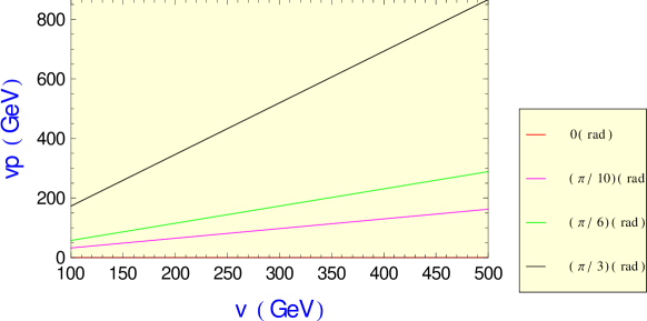
Figure 1: We show the values for $vp\equiv v^{\prime}_{L}$ as function of $v\equiv v_{L}$, using the first relation defined at Eq.(82), for $\beta=0,(\pi/10),(\pi/6),(\pi/3)$ rad as indicated at the box on right.

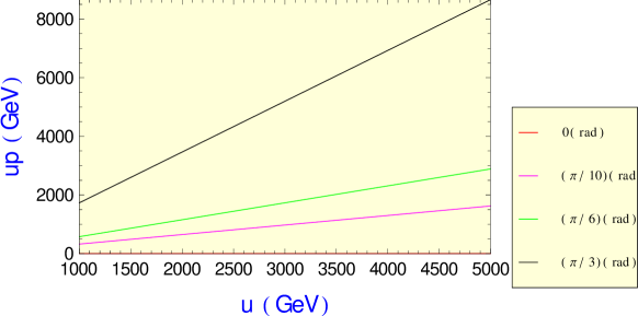
Figure 2: We show the values for $up\equiv v^{\prime}_{R}$ as function of $u\equiv v_{R}$, using the second relation defined at Eq.(82), for $\alpha=0,(\pi/10),(\pi/6),(\pi/3)$ rad as indicated at the box on right.

In our analyses we will consider

$$g=\sqrt{\frac{8G_{F}M^{2}_{W}}{\sqrt{2}}}=0.653,$$ (84)

the Standard Model gauge constant is the same as, it means $g_{L}\equiv g$ defined at Eq.(84). The experimental value of $W^{\pm}$-mass is given by:

$$M_{W^{\pm}}=80.379\pm 0.012\,\ {\mbox{G}eV},$$ (85)

Using Eqs.(81,84), we can get the following plot shown at Fig.(3), and it is the same as presented at [1], and we see we can get the $W^{\pm}$-mass values for all $\beta$-parameter and $140\leq v\leq 180$ (GeV), the exception is for $\beta=(\pi/3)$ rad.

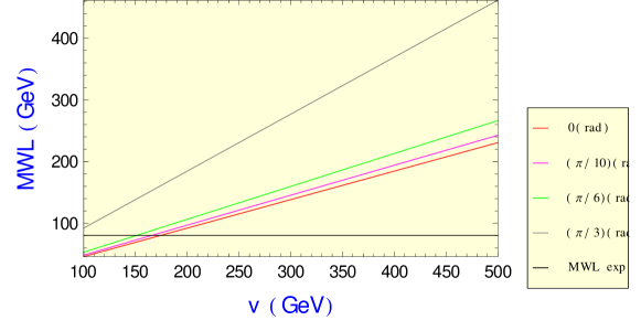
Figure 3: The masses of $W^{\pm}_{L}$ to several values of the $\beta$ parameter, with the same description give at Fig.(1). The black line means the experimental values of $M_{W^{\pm}}\equiv M_{W^{\pm}_{L}}$, see Eq.(85).

The experimental constraints for the new charged gauge boson is [15]:

$$M_{W^{\pm}_{R}}>2.7\,\ {\mbox{T}eV},$$ (86)

in this model we have three possibilities for $g_{R}$:

• $g_{R}>g_{L}$

  

  
  

  Figure 4: The masses of $W^{\pm}_{R}$ to several values of the $\alpha$ parameter, with the same description give at Fig.(2). The experimental constraints of $M_{W^{\pm}_{R}}$ is defined at Eq.(86).

• $g_{R}=g_{L}$

  

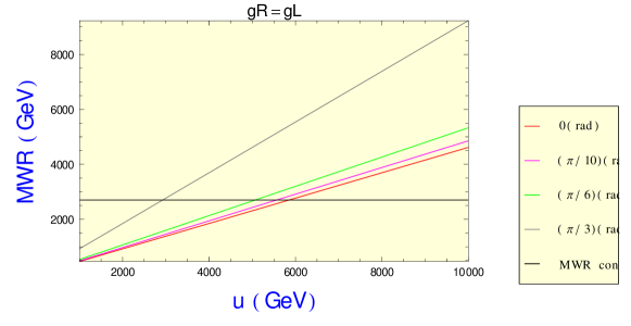
  Figure 5: The masses of $W^{\pm}_{R}$ to several values of the $\alpha$ parameter as in Fig.(4).

• $g_{R}<g_{L}$

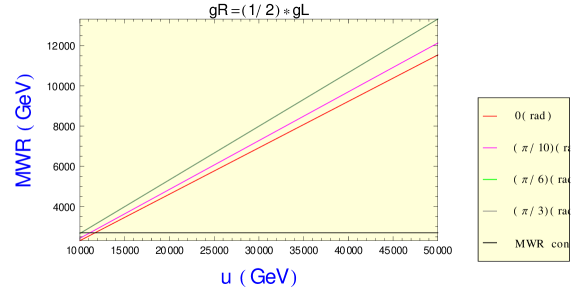
Figure 6: The masses of $W^{\pm}_{R}$ to several values of the $\alpha$ parameter as in Fig.(4).

Now the plot of the masses of $W^{\pm}_{R}$ is shown at Figs.(4,5,6) and they are in agreement with Eq.(83), see also Fig.(3), for $v_{R}>2000$ GeV.

5.2 Neutral Gauge Bosons

The mass matrix to the neutral gauge boson at the base $(V^{3L}_{m},V^{3R}_{m},V^{BL}_{m})$ is given by

$${\cal M}^{2}_{neu}=\left(\begin{array}[]{ccc}g^{2}_{L}(v_{L}^{2}+v_{L}^{\prime\,\ 2})&0&-g_{BL}g_{L}(v_{L}^{2}+v_{L}^{\prime\,\ 2})\\ 0&g^{2}_{R}(v_{R}^{2}+v_{R}^{\prime\,\ 2})&-g_{BL}g_{R}(v_{R}^{2}+v_{R}^{\prime\,\ 2})\\ -g_{BL}g_{L}(v_{L}^{2}+v_{L}^{\prime\,\ 2})&-g_{BL}g_{R}(v_{R}^{2}+v_{R}^{\prime\,\ 2})&g^{2}_{BL}(v_{L}^{2}+v_{L}^{\prime\,\ 2}+v_{R}^{2}+v_{R}^{\prime\,\ 2})\end{array}\right),$$ (87)

we get analytical the following result

$${\mbox{D}et}{\cal M}^{2}_{neu} = 0,$$

$${\mbox{T}r}{\cal M}^{2}_{neu} = g^{2}_{L}\left(v_{L}^{2}+v_{L}^{\prime\,\ 2}\right)+g^{2}_{R}\left(v_{R}^{2}+v_{R}^{\prime\,\ 2}\right)+g^{2}_{BL}\left(v_{L}^{2}+v_{L}^{\prime\,\ 2}+v_{R}^{2}+v_{R}^{\prime\,\ 2}\right),$$

this result is in agreement with the results presented at [5].

We have one non massive gauge boson, the photon, and two massive gauge bosons and they are $Z^{0}_{m},Z^{\prime 0}_{m}$. The photon is defined as

$$A^{0}_{m}=\sin\theta V^{3L}_{m}+\cos\theta\left(\sin\xi V^{3R}_{m}+\cos\xi V^{BL}_{m}\right),$$ (89)

where we have defined

$$\sin\theta = g_{BL}g_{R},\,\ \cos\theta=\sqrt{1-g^{2}_{BL}g^{2}_{R}},$$

$$\sin\xi = \frac{g_{BL}g_{L}}{\sqrt{1-g^{2}_{BL}g^{2}_{R}}},\,\ \cos\xi=\frac{g_{L}g_{R}}{\sqrt{1-g^{2}_{BL}g^{2}_{R}}}.$$ (90)

The gauge coupling must be related by

$$\frac{1}{e^{2}}=\frac{1}{g^{2}_{L}}+\frac{1}{g^{2}_{R}}+\frac{1}{g^{2}_{BL}},$$ (91)

therefore, we can conclude

$$g_{BL}=\frac{eg_{L}g_{R}}{\sqrt{g^{2}_{L}g^{2}_{R}-e^{2}g^{2}_{R}-e^{2}g^{2}_{L}}}.$$ (92)

Using Eq.(84) together with the equation above we get

$$g_{L} = g_{R}=0.652775,$$

$$g_{BL} = 0.121505.$$ (93)

The analytical results are so complicated, due it we will not reproduce it here. However, we have done some plots about the masses of both massive gauge bosons and our results are shown at Figs.(7,8). There are an experimental constraints for the masses of $Z^{\prime 0}$ and it is [15]

$$M_{Z^{\prime 0}}>1\,\ {\mbox{T}eV}.$$ (94)

for the case of $g_{L}=g_{R}$, while the experimental value of $Z^{0}$-mass is given by:

$$M_{Z^{0}}=91.1876\pm 0.0021\,\ {\mbox{G}eV}.$$ (95)

Figure 7: The masses of $Z^{0}$ to several values of the $\beta$ parameter in therms of the vev of $\phi_{L}$, the black line means the experimental constraints of $M_{Z^{0}}$ defined at Eq.(95).

Figure 8: The masses of $Z^{\prime 0}$ to several values of the $\alpha$ parameter in therms of the vev of $\phi_{R}$, the black line means the experimental constraints of $M_{Z^{\prime 0}}$ defined at Eq.(86).

6 Scalar Potential

In the non-SUSY model LRUSM, the scalar potential is given by [5]:

$$V = n^{2}_{L}|\phi_{L}|^{2}+n^{2}_{R}|\phi_{R}|^{2}+\lambda_{LL}\left(|\phi_{L}|^{2}\right)^{2}+\lambda_{RR}\left(|\phi_{R}|^{2}\right)^{2}+\lambda_{LR}\left(|\phi^{\dagger}_{L}\phi_{R}|^{2}\right)^{2}.$$

One year later they also included one singlet scalar field, see Eq.(27), and their main resultas are [6]:

• The Dine-Fischler-Srednicki role;

• The Chang-Mohapatra-Parida role;

• The Universal Seesaw Mechanism.

for the last result, see Eq.(28)

The scalar potential is written as

$$V_{MSUSM}=V_{D}+V_{F}+V_{\mbox{soft}}$$ (97)

where, see Eqs.(144,142,43), we can rewrite

$$V_{D} = -{\cal L}_{D}=\frac{1}{2}\left(D^{i}_{L}D^{i}_{L}+D^{i}_{R}D^{i}_{R}+D^{BL}D^{BL}\right)$$

$$= \frac{g^{2}_{L}}{8}\left[\left(|\phi_{L}|^{2}-|\phi^{\prime}_{L}|^{2}\right)^{2}+4|\phi^{\dagger\,\ \prime}_{L}\phi_{L}|^{2}\right]+\frac{g^{2}_{R}}{8}\left[\left(|\phi_{R}|^{2}-|\phi^{\prime}_{R}|^{2}\right)^{2}+4|\phi^{\dagger\,\ \prime}_{R}\phi_{R}|^{2}\right]$$

$$+ \frac{g^{2}_{BL}}{8}\left\{\left[\left(|\phi_{L}|^{2}-|\phi^{\prime}_{L}|^{2}\right)+\left(|\phi_{R}|^{2}-|\phi^{\prime}_{R}|^{2}\right)\right]^{2}+\left(|S|^{2}\right)^{2}-2\left(|\phi_{L}|^{2}-|\phi^{\prime}_{L}|^{2}\right)|S|^{2}\right.$$

$$- \left.2\left(|\phi_{R}|^{2}-|\phi^{\prime}_{R}|^{2}\right)|S|^{2}\right\},$$

$$V_{F} = -{\cal L}_{F}=\sum_{m}\bar{F}_{m}F_{m}$$

$$= |\mu_{L}|^{2}|\phi^{\prime}_{L}|^{2}+|\mu_{R}|^{2}|\phi^{\prime}_{R}|^{2}+|\mu_{L}|^{2}|\phi_{L}|^{2}+|\mu_{R}|^{2}|\phi_{R}|^{2}+|\mu_{S}|^{2}|S|^{2},$$

$$V_{soft} = -{\cal L}^{\mbox{scalar}}_{soft}$$ (98)

$$= M^{2}_{\phi_{L}}|\phi_{L}|^{2}+M^{2}_{\phi_{R}}|\phi_{R}|^{2}+M^{2}_{\phi^{\prime}_{L}}|\phi^{\prime}_{L}|^{2}+M^{2}_{\phi^{\prime}_{R}}|\phi^{\prime}_{R}|^{2}+M^{2}_{S}|S|^{2}-\left[\beta_{\phi_{L}}\left(\phi_{L}\phi^{\prime}_{L}\right)\right.$$

$$+ \left.\beta_{\phi_{R}}\left(\phi_{R}\phi^{\prime}_{R}\right)+\beta_{S}\left(S\right)^{2}+H.c.\right].$$

Therefore our scalar potential is given by:

$$V_{MSUSM} = m^{2}_{\phi_{L}}|\phi_{L}|^{2}+m^{2}_{\phi_{R}}|\phi_{R}|^{2}+m^{2}_{\phi^{\prime}_{L}}|\phi^{\prime}_{L}|^{2}+m^{2}_{\phi^{\prime}_{R}}|\phi^{\prime}_{R}|^{2}+m^{2}_{S}|S|^{2}-\left[\beta_{\phi_{L}}\left(\phi_{L}\phi^{\prime}_{L}\right)\right.$$ (99)

$$+ \left.\beta_{\phi_{R}}\left(\phi_{R}\phi^{\prime}_{R}\right)+\beta_{S}\left(S\right)^{2}+H.c.\right]+\frac{1}{8}\left(g^{2}_{L}+g^{2}_{BL}\right)\left(|\phi_{L}|^{2}-|\phi^{\prime}_{L}|^{2}\right)^{2}$$

$$+ \frac{1}{8}\left(g^{2}_{R}+g^{2}_{BL}\right)\left(|\phi_{R}|^{2}-|\phi^{\prime}_{R}|^{2}\right)^{2}+\frac{g^{2}_{L}}{2}|\phi^{\dagger\,\ \prime}_{L}\phi_{L}|^{2}+\frac{g^{2}_{R}}{2}|\phi^{\dagger\,\ \prime}_{R}\phi_{R}|^{2}$$

$$+ \frac{g^{2}_{BL}}{8}\left[2\left(|\phi_{L}|^{2}-|\phi^{\prime}_{L}|^{2}\right)\left(|\phi_{R}|^{2}-|\phi^{\prime}_{R}|^{2}\right)+\left(|S|^{2}\right)^{2}-2\left(|\phi_{L}|^{2}-|\phi^{\prime}_{L}|^{2}\right)|S|^{2}\right.$$

$$- \left.2\left(|\phi_{R}|^{2}-|\phi^{\prime}_{R}|^{2}\right)|S|^{2}\right].$$

where

$$m^{2}_{\phi_{L}} = M^{2}_{\phi_{L}}+|\mu_{L}|^{2},\,\ m^{2}_{\phi_{R}}=M^{2}_{\phi_{R}}+|\mu_{R}|^{2},$$

$$m^{2}_{\phi^{\prime}_{L}} = M^{2}_{\phi^{\prime}_{L}}+|\mu_{L}|^{2},\,\ m^{2}_{\phi^{\prime}_{R}}=M^{2}_{\phi^{\prime}_{R}}+|\mu_{R}|^{2},\,\ m^{2}_{S}=M^{2}_{S}+|\mu_{S}|^{2}.$$ (100)

All the five neutral scalar components $\phi^{0}_{L},\phi^{0}_{R},\phi^{\prime 0}_{L},\phi^{\prime 0}_{R},S$ gain non-zero vacuum expectation values. Making a shift in the neutral scalars as

$$<\phi_{L}> = \frac{1}{\sqrt{2}}\left(\begin{array}[]{c}v_{L}+H_{\phi_{L}}+\imath F_{\phi_{L}}\\ 0\end{array}\right)\,\ ,\,\ <\phi^{\prime}_{L}>=\frac{1}{\sqrt{2}}\left(\begin{array}[]{c}0\\ v^{\prime}_{L}+H_{\phi^{\prime}_{L}}+\imath F_{\phi^{\prime}_{L}}\par\end{array}\right)\,\ ,$$ (105)

$$<\phi_{R}> = \frac{1}{\sqrt{2}}\left(\begin{array}[]{c}v_{R}+H_{\phi_{R}}+\imath F_{\phi_{R}}\\ 0\end{array}\right)\,\ ,\,\ <\phi^{\prime}_{R}>=\frac{1}{\sqrt{2}}\left(\begin{array}[]{c}0\\ v^{\prime}_{R}+H_{\phi^{\prime}_{R}}+\imath F_{\phi^{\prime}_{R}}\end{array}\right)\,\ ,$$ (110)

$$<S> = \frac{1}{\sqrt{2}}\left(x+H_{S}+\imath F_{S}\right).$$ (111)

In the non-SUSY model LRUSM, the scalar potential is given by [5]:

$$V = n^{2}_{L}|\phi_{L}|^{2}+n^{2}_{R}|\phi_{R}|^{2}+\lambda_{LL}\left(|\phi_{L}|^{2}\right)^{2}+\lambda_{RR}\left(|\phi_{R}|^{2}\right)^{2}+\lambda_{LR}\left(|\phi^{\dagger}_{L}\phi_{R}|^{2}\right)^{2}.$$

One year later they also included one singlet scalar field, see Eq.(27), and their main resultas are [6]:

• The Dine-Fischler-Srednicki role;

• The Chang-Mohapatra-Parida role;

• The Universal Seesaw Mechanism.

The scalar potential is written as

$$V_{MSUSM}=V_{D}+V_{F}+V_{\mbox{soft}}$$ (113)

where, see Eqs.(144,142,43), we can rewrite

$$V_{D} = -{\cal L}_{D}=\frac{1}{2}\left(D^{i}_{L}D^{i}_{L}+D^{i}_{R}D^{i}_{R}+D^{BL}D^{BL}\right)$$

$$= \frac{g^{2}_{L}}{8}\left[\left(|\phi_{L}|^{2}-|\phi^{\prime}_{L}|^{2}\right)^{2}+4|\phi^{\dagger\,\ \prime}_{L}\phi_{L}|^{2}\right]+\frac{g^{2}_{R}}{8}\left[\left(|\phi_{R}|^{2}-|\phi^{\prime}_{R}|^{2}\right)^{2}+4|\phi^{\dagger\,\ \prime}_{R}\phi_{R}|^{2}\right]$$

$$+ \frac{g^{2}_{BL}}{8}\left\{\left[\left(|\phi_{L}|^{2}-|\phi^{\prime}_{L}|^{2}\right)+\left(|\phi_{R}|^{2}-|\phi^{\prime}_{R}|^{2}\right)\right]^{2}+\left(|S|^{2}\right)^{2}-2\left(|\phi_{L}|^{2}-|\phi^{\prime}_{L}|^{2}\right)|S|^{2}\right.$$

$$- \left.2\left(|\phi_{R}|^{2}-|\phi^{\prime}_{R}|^{2}\right)|S|^{2}\right\},$$

$$V_{F} = -{\cal L}_{F}=\sum_{m}\bar{F}_{m}F_{m}$$

$$= |\mu_{L}|^{2}|\phi^{\prime}_{L}|^{2}+|\mu_{R}|^{2}|\phi^{\prime}_{R}|^{2}+|\mu_{L}|^{2}|\phi_{L}|^{2}+|\mu_{R}|^{2}|\phi_{R}|^{2}+|\mu_{S}|^{2}|S|^{2},$$

$$V_{soft} = -{\cal L}^{\mbox{scalar}}_{soft}$$ (114)

$$= M^{2}_{\phi_{L}}|\phi_{L}|^{2}+M^{2}_{\phi_{R}}|\phi_{R}|^{2}+M^{2}_{\phi^{\prime}_{L}}|\phi^{\prime}_{L}|^{2}+M^{2}_{\phi^{\prime}_{R}}|\phi^{\prime}_{R}|^{2}+M^{2}_{S}|S|^{2}-\left[\beta_{\phi_{L}}\left(\phi_{L}\phi^{\prime}_{L}\right)\right.$$

$$+ \left.\beta_{\phi_{R}}\left(\phi_{R}\phi^{\prime}_{R}\right)+\beta_{S}\left(S\right)^{2}+H.c.\right].$$

Therefore our scalar potential is given by:

$$V_{MSUSM} = m^{2}_{\phi_{L}}|\phi_{L}|^{2}+m^{2}_{\phi_{R}}|\phi_{R}|^{2}+m^{2}_{\phi^{\prime}_{L}}|\phi^{\prime}_{L}|^{2}+m^{2}_{\phi^{\prime}_{R}}|\phi^{\prime}_{R}|^{2}+m^{2}_{S}|S|^{2}-\left[\beta_{\phi_{L}}\left(\phi_{L}\phi^{\prime}_{L}\right)\right.$$ (115)

$$+ \left.\beta_{\phi_{R}}\left(\phi_{R}\phi^{\prime}_{R}\right)+\beta_{S}\left(S\right)^{2}+H.c.\right]+\frac{1}{8}\left(g^{2}_{L}+g^{2}_{BL}\right)\left(|\phi_{L}|^{2}-|\phi^{\prime}_{L}|^{2}\right)^{2}$$

$$+ \frac{1}{8}\left(g^{2}_{R}+g^{2}_{BL}\right)\left(|\phi_{R}|^{2}-|\phi^{\prime}_{R}|^{2}\right)^{2}+\frac{g^{2}_{L}}{2}|\phi^{\dagger\,\ \prime}_{L}\phi_{L}|^{2}+\frac{g^{2}_{R}}{2}|\phi^{\dagger\,\ \prime}_{R}\phi_{R}|^{2}$$

$$+ \frac{g^{2}_{BL}}{8}\left[2\left(|\phi_{L}|^{2}-|\phi^{\prime}_{L}|^{2}\right)\left(|\phi_{R}|^{2}-|\phi^{\prime}_{R}|^{2}\right)+\left(|S|^{2}\right)^{2}-2\left(|\phi_{L}|^{2}-|\phi^{\prime}_{L}|^{2}\right)|S|^{2}\right.$$

$$- \left.2\left(|\phi_{R}|^{2}-|\phi^{\prime}_{R}|^{2}\right)|S|^{2}\right].$$

where

$$m^{2}_{\phi_{L}} = M^{2}_{\phi_{L}}+|\mu_{L}|^{2},\,\ m^{2}_{\phi_{R}}=M^{2}_{\phi_{R}}+|\mu_{R}|^{2},$$

$$m^{2}_{\phi^{\prime}_{L}} = M^{2}_{\phi^{\prime}_{L}}+|\mu_{L}|^{2},\,\ m^{2}_{\phi^{\prime}_{R}}=M^{2}_{\phi^{\prime}_{R}}+|\mu_{R}|^{2},\,\ m^{2}_{S}=M^{2}_{S}+|\mu_{S}|^{2}.$$ (116)

All the five neutral scalar components $\phi^{0}_{L},\phi^{0}_{R},\phi^{\prime 0}_{L},\phi^{\prime 0}_{R},S$ gain non-zero vacuum expectation values. Making a shift in the neutral scalars as

$$<\phi_{L}> = \frac{1}{\sqrt{2}}\left(\begin{array}[]{c}v_{L}+H_{\phi_{L}}+\imath F_{\phi_{L}}\\ 0\end{array}\right)\,\ ,\,\ <\phi^{\prime}_{L}>=\frac{1}{\sqrt{2}}\left(\begin{array}[]{c}0\\ v^{\prime}_{L}+H_{\phi^{\prime}_{L}}+\imath F_{\phi^{\prime}_{L}}\par\end{array}\right)\,\ ,$$ (121)

$$<\phi_{R}> = \frac{1}{\sqrt{2}}\left(\begin{array}[]{c}v_{R}+H_{\phi_{R}}+\imath F_{\phi_{R}}\\ 0\end{array}\right)\,\ ,\,\ <\phi^{\prime}_{R}>=\frac{1}{\sqrt{2}}\left(\begin{array}[]{c}0\\ v^{\prime}_{R}+H_{\phi^{\prime}_{R}}+\imath F_{\phi^{\prime}_{R}}\end{array}\right)\,\ ,$$ (126)

$$<S> = \frac{1}{\sqrt{2}}\left(x+H_{S}+\imath F_{S}\right).$$ (127)

7 Constraint Equations

Here in this section we give the constraint equations, due to the requirement the potential to reach a minimum at the chosen VEV’s. We get this equation requiring that in the shifted potential the linear terms in fields must be absent

$$8v_{L}M^{2}_{\phi_{L}} = 8\beta_{\phi_{L}}v^{\prime}_{L}+v_{L}\left[(g^{2}_{L}+g^{2}_{BL})(v^{\prime 2}_{L}-v^{2}_{L})+g^{2}_{BL}(v^{\prime 2}_{R}-v^{2}_{R})+8(x^{2}-\mu^{2}_{L})\right],$$

$$8v_{R}M^{2}_{\phi_{R}} = -8\beta_{\phi_{R}}v^{\prime}_{R}+v_{R}\left[(g^{2}_{R}+g^{2}_{BL})(v^{\prime 2}_{R}-v^{2}_{R})+g^{2}_{BL}(v^{\prime 2}_{L}-v^{2}_{L})+8(x^{2}-\mu^{2}_{R})\right],$$

$$8v^{\prime}_{L}M^{2}_{\phi^{\prime}_{L}} = -8\beta_{\phi_{L}}v_{L}-v^{\prime}_{L}\left[g^{2}_{BL}(v^{\prime 2}_{R}-v^{2}_{R})+(g^{2}_{L}+g^{2}_{BL})(v^{\prime 2}_{L}-v^{2}_{L})-8(x^{2}+\mu^{2}_{L})\right],$$

$$8v^{\prime}_{R}M^{2}_{\phi^{\prime}_{R}} = 8\beta_{\phi_{R}}v_{R}+v^{\prime}_{R}\left[g^{2}_{BL}(v^{2}_{L}-v^{\prime 2}_{L})+(g^{2}_{R}+g^{2}_{BL})(v^{2}_{R}-v^{\prime 2}_{R})-8(x^{2}+\mu^{2}_{R})\right],$$

$$M^{2}_{S} = 2\beta_{S}+v^{2}_{L}+v^{2}_{R}-v^{\prime 2}_{L}-v^{\prime 2}_{R}-x^{2}-\mu^{2}_{S}.$$ (128)

The mass matrices, thus, can be calculated, using

$$M_{ij}^{2}=\frac{\partial^{2}V_{MSUSY331}}{\partial\phi_{i}\partial\phi_{j}}$$ (129)

evaluated at the chosen minimum, where $\phi_{i}$ are the scalars of our model described above.

For the sake of simplicity, here we assume that vacuum expectation values (VEVs) are real. This means that the CP violation through the scalar exchange is not considered in this work. In literature, a real part $H$ is called CP-even scalar or scalar, and an imaginary one $F$ - CP-odd scalar or pseudoscalar field. In this paper we call them scalar and pseudoscalar, respectively.

8 Mass Spectrum general case

We can write, from Eqs.(82, 154, 164, 190), the following expression for our light $CP$-even, $CP$-odd and Charged scalars:

$$M_{H^{0}_{1}} = \sqrt{\left(\frac{g^{2}_{L}+g^{2}_{BL}}{4}\right)v^{2}_{L}\sec\beta+\left(\frac{g^{2}_{R}+g^{2}_{BL}}{4}\right)v^{2}_{R}\sec\alpha},$$

$$m_{A^{0}_{1}} = \beta_{\phi_{L}}\sqrt{\frac{2}{\sin\left(2\beta\right)}},\,\ m_{A^{0}_{2}}=\beta_{\phi_{R}}\sqrt{\frac{2}{\sin\left(2\alpha\right)}},$$

$$m_{H^{\pm}_{1}} = \sqrt{\left[\frac{\beta^{2}_{\phi_{L}}}{\tan\beta}+\frac{g^{2}_{L}}{4}v^{2}_{L}\right]\sec\beta}.$$ (130)

We have discussed that the masses of those light scalars are very similar to ones at MSSM [1]. The $\beta$-parameter has to satisfy the following constraints

$$\beta \neq 0\,\ \mbox{rad},\,\ \mbox{and}\,\ \beta\neq\frac{\pi}{2}\,\ \mbox{rad},$$

$$0 < \beta<\frac{\pi}{2}\,\ \mbox{rad},$$ (131)

and $\alpha$-parameter also has to satisfy those condition above presented. However on this model the following relations hold in MSSM [1]

$$m^{2}_{H^{\pm}} = m^{2}_{A^{0}}+M^{2}_{W^{\pm}},$$

$$m^{2}_{h^{0}}+m^{2}_{H^{0}} = m^{2}_{A^{0}}+M^{2}_{Z^{0}}.$$ (132)

are not hold in our model.

Using Eqs.(84,93) at Eqs.(164,190) and we use $\beta_{\phi_{L}}=2000$ GeV; $\beta_{\phi_{R}}=3000$ GeV and $\beta_{S}=2500$ GeV; we get the following masses values for the masses of our scalars:

$$m_{A^{0}_{1}} = 3039.34\,\ \mbox{GeV},\,\ m_{A^{0}_{2}}=4559.01\,\ \mbox{GeV},\,\ m_{A^{0}_{3}}=5000\,\ \mbox{GeV},$$

$$m_{H^{\pm}_{1}} = 3039.68\,\ \mbox{GeV},\,\ m_{H^{\pm}_{2}}=4561.93\,\ \mbox{GeV},$$ (133)

those values are in agreement with the experimental limits for new scalars defined as

$$m_{A^{0}} > 863\,\ \mbox{GeV},\,\ m_{H^{+}}>181\,\ \mbox{GeV},$$

at $\tan\beta=10$ [15].

We have done at Fig.(1) plots for $\beta=0,(\pi/10),(\pi/6),(\pi/3)$ rad but considerating the Eq.(131) we will not use the first values and due the fact that $\tan\left(\frac{\pi}{6}\right)=\cot\left(\frac{\pi}{3}\right)$ we will also not present the last value for $\beta$ and $\alpha$-parameters when we present our plots to the scalars masses.

We show at Figs.(9,10) the masses of pseudo and charged Higgs as funtion of $\beta_{\phi_{L}}$. We can conclude when we consider $v_{L}=120$ GeV we can get masses four our light pseudo-scalar and also charged scalar bigger than the experimental constraints.

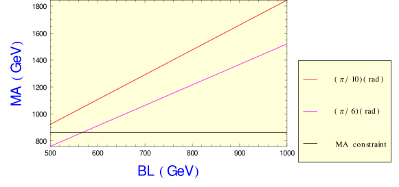
Figure 9: The masses of $A$ to several values of the $\beta$ parameter, for $\beta=(\pi/10),(\pi/6)$ rad and $v_{L}=120$ GeV; in therms of the soft parameter of $L$. The black line means the experimental constraints of $M_{A}$ defined at Eq.(LABEL:expresultas).

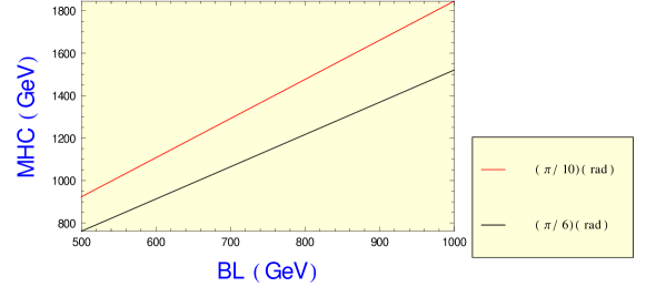
Figure 10: The masses of $H^{\pm}$ to several values of the $\beta$ parameter in similar way as done at Fig.(9).

Our results for the light Higgs bosons are shown at Figs.(11,12), and we see that we can reproduce for our light Higgs boson the experimental values of light Higgs Boson is [15]:

$$m_{H^{0}_{1}}=125.10\pm 0.14\,\ \mbox{GeV}.$$ (135)

Figure 11: The masses of $H^{0}_{1}$ to several values of the $\beta$ parameter and $\alpha=(\pi/3)$ in therms of the soft parameter of $v_{R}\equiv u$, the black line means the experimental constraints of $M_{H^{0}_{1}}$ defined at Eq.(135).

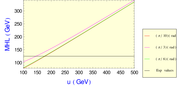
Figure 12: The masses of $H^{0}_{1}$ to several values of the $\alpha$ parameter and $\beta=(\pi/3)$ in therms of the soft parameter of $v_{L}\equiv v$, the black line means the experimental constraints of $M_{H^{0}_{1}}$ defined at Eq.(135).

9 Conclusions

In this article we constructed the Supersymmetric version of the Universal Seesaw Mechanism. We have presented the model, considerating only one familly fermion coupling with the usual Scalars in such way we can explain the mixing data. We have also performed numerical analyses of the gauge boson masses and we also have get the masses for all usual scalar particles. All the mass spectrum are in agreement with the experimental limits, as discussed above.

Appendix A Eliminating the Auxiliar Fields

To get the scalar potential of our model we have to eliminate the auxiliarly fields $F$ and $D$ that appear in our model. We are going to pick up the $F$ and $D$- terms, from Eqs.(36,38,LABEL:sp3m1), we get

$${\cal L}^{gauge}_{D} = \frac{1}{2}\left(D^{i}_{L}D^{i}_{L}+D^{i}_{R}D^{i}_{R}+D^{BL}D^{BL}\right),$$

$${\cal L}^{scalar}_{F} = |F_{\phi_{L}}|^{2}+|F_{\phi_{R}}|^{2}+|F_{\phi^{\prime}_{L}}|^{2}+|F_{\phi^{\prime}_{R}}|^{2}+|F_{S}|^{2},$$

$${\cal L}^{scalar}_{D} = \frac{g_{L}}{2}\left[\bar{\phi}_{L}\sigma^{i}\phi_{L}+\bar{\phi}^{\prime}_{L}\sigma^{i}\phi^{\prime}_{L}\right]D^{i}_{L}+\frac{g_{R}}{2}\left[\bar{\phi}_{R}\sigma^{i}\phi_{R}+\bar{\phi}^{\prime}_{R}\sigma^{i}\phi^{\prime}_{R}\right]D^{i}_{R}$$

$$+ \frac{g_{BL}}{2}\left[-|\phi_{L}|^{2}-|\phi_{R}|^{2}+|\phi^{\prime}_{L}|^{2}+|\phi^{\prime}_{R}|^{2}+|F_{S}|{2}\right]D^{BL},$$

$${\cal L}^{W2}_{F} = \mu_{L}\left(\phi_{L}F_{\phi^{\prime}_{L}}+F_{\prime_{L}}\phi^{\prime}_{L}+\bar{\phi}_{L}\bar{F}_{\phi^{\prime}_{L}}+\bar{F}_{\prime_{L}}\overline{\phi^{\prime}}_{L}\right)$$

$$+ \mu_{R}\left(\phi_{R}F_{\phi^{\prime}_{R}}+F_{\prime_{R}}\phi^{\prime}_{R}+\bar{\phi}_{R}\bar{F}_{\phi^{\prime}_{R}}+\bar{F}_{\prime_{R}}\overline{\phi^{\prime}}_{R}\right)$$

$$+ \mu_{S}\left(SF_{S}+\bar{S}\bar{F}_{S}\right).$$

Our $R$-parity, defined at Tab.(5), eliminate the followings terms in our superpotential

$$\frac{\kappa}{3}\hat{S}\hat{S}\hat{S}+\lambda_{L}\left(\hat{\phi}_{L}\hat{\phi}^{\prime}_{L}\right)\hat{S}+\lambda_{R}\left(\hat{\phi}_{R}\hat{\phi}^{\prime}_{R}\right)\hat{S}$$ (137)

those terms would give the following contribute to eliminate the $F$-terms

$${\cal L}^{W3}_{F} = \kappa F_{S}S^{2}+\lambda_{L}\left(F_{\phi_{L}}\phi^{\prime}_{L}S+\phi_{L}F_{\phi^{\prime}_{L}}S+\phi_{L}\phi^{\prime}_{L}F_{S}\right)$$ (138)

$$+ \lambda_{R}\left(F_{\phi_{R}}\phi^{\prime}_{R}S+\phi_{R}F_{\phi^{\prime}_{R}}S+\phi_{R}\phi^{\prime}_{R}F_{S}\right).$$

From the equation described above we can construct

$${\cal L}_{F} = {\cal L}^{scalar}_{F}+{\cal L}^{W2}_{F}$$

$$= |F_{\phi_{L}}|^{2}+|F_{\phi_{R}}|^{2}+|F_{\phi^{\prime}_{L}}|^{2}+|F_{\phi^{\prime}_{R}}|^{2}+|F_{S}|^{2}+\mu_{L}\left(\phi_{L}F_{\phi^{\prime}_{L}}+F_{\prime_{L}}\phi^{\prime}_{L}+\bar{\phi}_{L}\bar{F}_{\phi^{\prime}_{L}}+\bar{F}_{\prime_{L}}\overline{\phi^{\prime}}_{L}\right)$$

$$+ \mu_{R}\left(\phi_{R}F_{\phi^{\prime}_{R}}+F_{\prime_{R}}\phi^{\prime}_{R}+\bar{\phi}_{R}\bar{F}_{\phi^{\prime}_{R}}+\bar{F}_{\prime_{R}}\overline{\phi^{\prime}}_{R}\right)$$

$$+ \mu_{S}\left(SF_{S}+\bar{S}\bar{F}_{S}\right)\,\ ,$$

$${\cal L}_{D} = {\cal L}^{gauge}_{D}+{\cal L}^{scalar}_{D}$$

$$= \frac{1}{2}\left(D^{i}_{L}D^{i}_{L}+D^{i}_{R}D^{i}_{R}+D^{BL}D^{BL}\right)+\frac{g_{L}}{2}\left[\bar{\phi}_{L}\sigma^{i}\phi_{L}+\bar{\phi}^{\prime}_{L}\sigma^{i}\phi^{\prime}_{L}\right]D^{i}_{L}$$

$$+ \frac{g_{R}}{2}\left[\bar{\phi}_{R}\sigma^{i}\phi_{R}+\bar{\phi}^{\prime}_{R}\sigma^{i}\phi^{\prime}_{R}\right]D^{i}_{R}+\frac{g_{BL}}{2}\left[-|\phi_{L}|^{2}-|\phi_{R}|^{2}+|\phi^{\prime}_{L}|^{2}+|\phi^{\prime}_{R}|^{2}+|S|{2}\right]D^{BL}.$$

We will now show that these fields can be eliminated through the Euler-Lagrange equations

$$\frac{\partial{\cal L}}{\partial\phi}-\partial_{m}\frac{\partial{\cal L}}{\partial(\partial_{m}\phi)}=0\,\ ,$$ (140)

where $\phi=\phi_{L},\phi_{R},\phi^{\prime}_{L},\phi^{\prime}_{R},S$. Formally auxiliary fields are defined as fields having no kintetic terms. Thus, this definition immediately yields that the Euler-Lagrange equations for auxiliary fields simplify to $\frac{\partial{\cal L}}{\partial\phi}=0$.

Applying these simplified equations to various auxiliary $F$-fields yields the following relations

$$\bar{F}_{\phi_{L}} = -\bar{\mu}_{L}\phi^{\prime}_{L}\,\ ;\,\ F_{\phi_{L}}=-\mu_{L}\overline{\phi^{\prime}}_{L},$$

$$\bar{F}_{\phi_{R}} = -\bar{\mu}_{R}\phi^{\prime}_{R}\,\ ;\,\ F_{\phi_{R}}=-\mu_{R}\overline{\phi^{\prime}}_{R},$$

$$\bar{F}_{\phi^{\prime}_{L}} = -\bar{\mu}_{L}\phi_{L}\,\ ;\,\ F_{\phi^{\prime}_{L}}=-\mu_{L}\bar{\phi}_{L},$$

$$\bar{F}_{\phi^{\prime}_{R}} = -\mu_{R}\phi_{R}\,\ ;\,\ F_{\phi^{\prime}_{R}}=-\bar{\mu}_{R}\overline{\phi}_{R},$$

$$\bar{F}_{S} = -\mu_{S}S\,\ ;\,\ F_{S}=-\bar{\mu}_{S}\bar{S}\,\ ,$$ (141)

using these equations, we can rewrite Eq.(LABEL:auxiliarm1) as

$${\cal L}_{F} = -\left(|F_{\phi_{L}}|^{2}+|F_{\phi_{R}}|^{2}+|F_{\phi^{\prime}_{L}}|^{2}+|F_{\phi^{\prime}_{R}}|^{2}+|F_{S}|^{2}\right)$$ (142)

$$= |\mu_{L}|^{2}|\phi^{\prime}_{L}|^{2}+|\mu_{R}|^{2}|\phi^{\prime}_{R}|^{2}+|\mu_{L}|^{2}|\phi_{L}|^{2}+|\mu_{R}|^{2}|\phi_{R}|^{2}+|\mu_{S}|^{2}|S|^{2}.$$

If we perform the same program to $D$-fields we get

$$D^{i}_{L} = -\frac{g_{L}}{2}\left[\bar{\phi}_{L}\sigma^{i}\phi_{L}+\bar{\phi}^{\prime}_{L}\sigma^{i}\phi^{\prime}_{L}\right]\,\ ,$$

$$D^{i}_{R} = -\frac{g_{R}}{2}\left[\bar{\phi}_{R}\sigma^{i}\phi_{R}+\bar{\phi}^{\prime}_{R}\sigma^{i}\phi^{\prime}_{R}\right]\,\ ,$$

$$D^{BL} = -\frac{g_{BL}}{2}\left[-|\phi_{L}|^{2}-|\phi_{R}|^{2}+|\phi^{\prime}_{L}|^{2}+|\phi^{\prime}_{R}|^{2}+|S|^{2}\right]\,\ ,$$ (143)

According with Eq.(LABEL:auxiliarm1)

$${\cal L}_{D} = -\frac{1}{2}\left(D^{i}_{L}D^{i}_{L}+D^{i}_{R}D^{i}_{R}+D^{BL}D^{BL}\right)$$ (144)

$$= -\frac{g^{2}_{L}}{8}\left[\left(|\phi_{L}|^{2}-|\phi^{\prime}_{L}|^{2}\right)^{2}+4|\phi^{\dagger\,\ \prime}_{L}\phi_{L}|^{2}\right]-\frac{g^{2}_{R}}{8}\left[\left(|\phi_{R}|^{2}-|\phi^{\prime}_{R}|^{2}\right)^{2}+4|\phi^{\dagger\,\ \prime}_{R}\phi_{R}|^{2}\right]$$

$$- \frac{g^{2}_{BL}}{8}\left\{\left[\left(|\phi_{L}|^{2}-|\phi^{\prime}_{L}|^{2}\right)+\left(|\phi_{R}|^{2}-|\phi^{\prime}_{R}|^{2}\right)\right]^{2}+\left(|S|^{2}\right)^{2}-2\left(|\phi_{L}|^{2}-|\phi^{\prime}_{L}|^{2}\right)|S|^{2}\right.$$

$$- \left.2\left(|\phi_{R}|^{2}-|\phi^{\prime}_{R}|^{2}\right)|S|^{2}\right\},$$

we have used the relation

$$\vec{\sigma}_{AB}\cdot\vec{\sigma}_{CD}=2\delta_{AD}\delta_{BC}-\delta_{AB}\delta_{CD}.$$ (145)

Appendix B Scalar in MSUSM.

Calculating Eq.(115) with the help of Eqs.(127,128) and using as base the following set of scalars $H_{\phi_{L}},H_{\phi_{R}},H_{\phi^{\prime}_{L}},H_{\phi^{\prime}_{R}},H_{S}$, the mass matrix, with the help of Eq.(128), the mass matrix is written as

$${\cal M}^{2}_{CP-even} = \left(\begin{array}[]{ccccc}{\bf{\cal M}^{even}_{11}}&{\bf{\cal M}^{even}_{12}}&{\bf{\cal M}^{even}_{13}}&{\bf{\cal M}^{even}_{14}}&{\bf{\cal M}^{even}_{15}}\\ {\bf{\cal M}^{even}_{12}}&{\bf{\cal M}^{even}_{22}}&{\bf{\cal M}^{even}_{23}}&{\bf{\cal M}^{even}_{24}}&{\bf{\cal M}^{even}_{25}}\\ {\bf{\cal M}^{even}_{13}}&{\bf{\cal M}^{even}_{23}}&{\bf{\cal M}^{even}_{33}}&{\bf{\cal M}^{even}_{34}}&{\bf{\cal M}^{even}_{35}}\\ {\bf{\cal M}^{even}_{14}}&{\bf{\cal M}^{even}_{24}}&{\bf{\cal M}^{even}_{34}}&{\bf{\cal M}^{even}_{44}}&{\bf{\cal M}^{even}_{45}}\\ {\bf{\cal M}^{even}_{15}}&{\bf{\cal M}^{even}_{25}}&{\bf{\cal M}^{even}_{35}}&{\bf{\cal M}^{even}_{45}}&{\bf{\cal M}^{even}_{55}}\end{array}\right)$$ (151)

where we have defined:

$${\bf{\cal M}^{even}_{11}} = \left(\frac{g^{2}_{L}+g^{2}_{BL}}{4}\right)v^{2}_{L}+\beta^{2}_{\phi_{L}}\frac{v^{\prime}_{L}}{v_{L}},\,\ {\bf{\cal M}^{even}_{12}}=\frac{g^{2}_{BL}}{4}v_{L}v_{R},$$

$${\bf{\cal M}^{even}_{13}} = -\beta^{2}_{\phi_{L}}+\left(\frac{g^{2}_{L}+g^{2}_{BL}}{4}\right)v_{L}v^{\prime}_{L},\,\ {\bf{\cal M}^{even}_{14}}=-\frac{g^{2}_{BL}}{4}v_{L}v^{\prime}_{R},\,\ {\bf{\cal M}^{even}_{15}}=-2xv_{L},$$

$${\bf{\cal M}^{even}_{22}} = \left(\frac{g^{2}_{R}+g^{2}_{BL}}{4}\right)v^{2}_{R}+\beta^{2}_{\phi_{R}}\frac{v^{\prime}_{R}}{v_{R}},\,\ {\bf{\cal M}^{even}_{23}}=\frac{g^{2}_{BL}}{4}v_{R}v^{\prime}_{L},$$

$${\bf{\cal M}^{even}_{24}} = -\beta^{2}_{\phi_{R}}-\left(\frac{g^{2}_{R}+g^{2}_{BL}}{4}\right)v_{R}v^{\prime}_{R},\,\ {\bf{\cal M}^{even}_{25}}=-2xvv_{R},$$

$${\bf{\cal M}^{even}_{33}} = \left(\frac{g^{2}_{L}+g^{2}_{BL}}{4}\right)v^{\prime 2}_{L}+\beta^{2}_{\phi_{L}}\frac{v_{L}}{v^{\prime}_{L}},\,\ {\bf{\cal M}^{even}_{34}}=\frac{g^{2}_{BL}}{4}v^{\prime}_{L}v^{\prime}_{R},\,\ {\bf{\cal M}^{even}_{35}}=2xv^{\prime}_{L},$$

$${\bf{\cal M}^{even}_{44}} = \left(\frac{g^{2}_{R}+g^{2}_{BL}}{4}\right)v^{\prime 2}_{R}+\beta^{2}_{\phi_{R}}\frac{v_{R}}{v^{\prime}_{R}},\,\ {\bf{\cal M}^{even}_{45}}=2xv^{\prime}_{R},$$

$${\bf{\cal M}^{even}_{45}} = 2x^{2}.$$ (152)

It is easy to show the following results

$${\mbox{D}et}{\cal M}^{2}_{CP-even} = \frac{1}{8v_{L}v_{R}v^{\prime}_{L}v^{\prime}_{R}}\left\{\beta^{2}_{\phi_{L}}\beta^{2}_{\phi_{R}}\left[\left(g^{2}_{BL}-8\right)g^{2}_{R}+\left(g^{2}_{BL}-8+g^{2}_{R}\right)g^{2}_{L}\right]\right.$$

$$\times \left.\left(v^{2}_{L}+v^{\prime 2}_{L}\right)\left(v^{\prime 2}_{R}-v^{2}_{R}\right)x^{2}\right\},$$

$${\mbox{T}r}{\cal M}^{2}_{CP-even} = \left(\frac{g^{2}_{L}+g^{2}_{BL}}{4}\right)\left(v^{2}_{L}+v^{\prime 2}_{L}\right)+\left(\frac{g^{2}_{R}+g^{2}_{BL}}{4}\right)\left(v^{2}_{R}+v^{\prime 2}_{R}\right)$$

$$+ \beta^{2}_{\phi_{L}}\left(\frac{v_{L}}{v^{\prime}_{L}}+\frac{v^{\prime}_{L}}{v_{L}}\right)+\beta^{2}_{\phi_{R}}\left(\frac{v_{R}}{v^{\prime}_{R}}+\frac{v^{\prime}_{R}}{v_{R}}\right)+2x^{2}.$$

This matrix has no Goldstone bosons and five mass eigenstates, which we denote as $H^{0}_{1},H^{0}_{2},H^{0}_{3},H^{0}_{4},H^{0}_{5}$.

We can using Eq.(LABEL:dettrcp-even), get the following expression for our light CP-even boson

$$M_{H^{0}_{1}} = \sqrt{\left(\frac{g^{2}_{L}+g^{2}_{BL}}{4}\right)\left(v^{2}_{L}+v^{\prime 2}_{L}\right)+\left(\frac{g^{2}_{R}+g^{2}_{BL}}{4}\right)\left(v^{2}_{R}+v^{\prime 2}_{R}\right)}$$ (154)

$$= \sqrt{\left(\frac{g^{2}_{L}+g^{2}_{BL}}{4}\right)v^{2}_{L}\left(1+\tan^{2}\beta\right)+\left(\frac{g^{2}_{R}+g^{2}_{BL}}{4}\right)v^{2}_{R}\left(1+\tan^{2}\alpha\right)},$$

where we have used Eq.(82).

Appendix C Pseudoscalar in MSUSM.

On this case using the base given by $F_{\phi_{L}},F_{\phi_{R}},F_{\phi^{\prime}_{L}},F_{\phi^{\prime}_{R}},F_{S}$, the mass matrix, with the help of Eq.(128), the mass matrix is written as

$${\cal M}^{2}_{CP-odd} = \left(\begin{array}[]{ccccc}{\bf{\cal M}^{odd}_{11}}&0&{\bf{\cal M}^{odd}_{13}}&0&0\\ 0&{\bf{\cal M}^{odd}_{22}}&0&{\bf{\cal M}^{odd}_{24}}&0\\ {\bf{\cal M}^{odd}_{13}}&0&{\bf{\cal M}^{odd}_{33}}&0&0\\ 0&{\bf{\cal M}^{odd}_{24}}&0&{\bf{\cal M}^{odd}_{44}}&0\\ 0&0&0&0&{\bf{\cal M}^{odd}_{55}}\end{array}\right)$$ (160)

where we have defined:

$${\bf{\cal M}^{odd}_{11}} = \beta^{2}_{\phi_{L}}\frac{v^{\prime}_{L}}{v_{L}},\,\ {\bf{\cal M}^{odd}_{13}}=\beta^{2}_{\phi_{L}},\,\ {\bf{\cal M}^{odd}_{22}}=\beta^{2}_{\phi_{R}}\frac{v^{\prime}_{R}}{v_{R}},\,\ {\bf{\cal M}^{odd}_{24}}=\beta^{2}_{\phi_{L}},$$

$${\bf{\cal M}^{odd}_{33}} = \beta^{2}_{\phi_{L}}\frac{v_{L}}{v^{\prime}_{L}},\,\ {\bf{\cal M}^{odd}_{44}}=\beta^{2}_{\phi_{R}}\frac{v_{R}}{v^{\prime}_{R}},\,\ {\bf{\cal M}^{odd}_{55}}=\beta^{2}_{\phi_{S}}.$$ (161)

Note that the basis $(F_{\phi_{L}},F_{\phi^{\prime}_{L}})$ does not mix with $(F_{\phi_{R}},F_{\phi^{\prime}_{R}}$ neither with $(F_{S})$.

It is easy to show the following results

$${\mbox{D}et}{\cal M}^{2}_{CP-odd} = 0,$$

$${\mbox{T}r}{\cal M}^{2}_{CP-odd} = 4\beta^{2}_{\phi_{S}}+\beta^{2}_{\phi_{L}}\left(\tan\beta+\cot\beta\right)+\beta^{2}_{\phi_{R}}\left(\tan\alpha+\cot\alpha\right),$$

where the characteristic equation is given by:

$$x^{2}\left(4\beta^{2}_{\phi_{S}}\right)\left(\beta^{2}_{\phi_{\phi_{L}}}(v^{2}_{L}+v^{\prime 2}_{L})-v_{L}v^{\prime}_{L}x\right)\left(\beta^{2}_{\phi_{\phi_{R}}}(v^{2}_{R}+v^{\prime 2}_{R})-v_{R}v^{\prime}_{R}x\right)=0.$$ (163)

This mass matrix has two Goldstone bosons,$G^{0}_{1},G^{0}_{2}$ (they will become the longitudinal components of the $Z^{0}_{m}$ and $Z^{\prime 0}_{m}$ neutral vector bosons).

We have also three mass eigenstates, $A^{0}_{1},A^{0}_{2},A^{0}_{3}$ and their masses are given by:

$$m^{2}_{A^{0}_{1}} = \beta^{2}_{\phi_{L}}\left(\tan\beta+\cot\beta\right)\gg M^{2}_{Z},$$

$$m^{2}_{A^{0}_{2}} = \beta^{2}_{\phi_{R}}\left(\tan\alpha+\cot\alpha\right)\gg M^{2}_{Z^{\prime}},$$

$$m^{2}_{A^{0}_{3}} = 4\beta_{\phi_{S}}.$$ (164)

see Eq.(LABEL:neutralgaugebosonsmasses). The pseudo-scalar scalar at MSSM has the following mass expression [1]:

$$M^{2}_{A^{0}} = M^{2}_{12}\left(\tan\beta+\cot\beta\right),$$ (165)

and its values is similar expression for our $m^{2}_{A^{0}_{1}}$.

Therefore, the mass eigenstates can be defined as:

$$\left(\begin{array}[]{c}G^{0}_{1}\\ A^{0}_{1}\\ G^{0}_{2}\\ A^{0}_{2}\\ A^{0}_{3}\end{array}\right) = \left(\begin{array}[]{ccccc}\cos\beta&\sin\beta&0&0&0\\ -\sin\beta&\cos\beta&0&0&0\\ 0&0&\cos\alpha&\sin\alpha&0\\ 0&0&-\sin\alpha&\cos\alpha&0\\ 0&0&0&0&1\end{array}\right)\left(\begin{array}[]{c}F_{\phi_{L}}\\ F_{\phi^{\prime}_{L}}\\ F_{\phi_{R}}\\ F_{\phi^{\prime}_{R}}\\ F_{S}\end{array}\right).$$ (181)

Appendix D Charged fields in MSUSM.

On this case the basis is given by $\phi^{\pm}_{L},\phi^{\pm}_{R},\phi^{\prime\pm}_{L},\phi^{\prime\pm}_{R}$, with the help of Eq.(128), we get the mass matrix is written as

$${\cal M}^{2}_{Charged} = \left(\begin{array}[]{cccc}{\bf{\cal M}^{charg}_{11}}&0&{\bf{\cal M}^{charg}_{13}}&0\\ 0&{\bf{\cal M}^{charg}_{22}}&0&{\bf{\cal M}^{charg}_{24}}\\ {\bf{\cal M}^{charg}_{13}}&0&{\bf{\cal M}^{charg}_{33}}&0\\ 0&{\bf{\cal M}^{charg}_{24}}&0&{\bf{\cal M}^{charg}_{44}}\end{array}\right)$$ (186)

where we have defined:

$${\bf{\cal M}^{charg}_{11}} = \beta^{2}_{\phi_{L}}\frac{v^{\prime}_{L}}{v_{L}}+\frac{g^{2}_{L}}{4}v^{\prime 2}_{L},\,\ {\bf{\cal M}^{charg}_{13}}=\beta^{2}_{\phi_{L}}+\frac{g^{2}_{L}}{4}v^{\prime}_{L}v_{L},$$

$${\bf{\cal M}^{charg}_{22}} = \beta^{2}_{\phi_{R}}\frac{v^{\prime}_{R}}{v_{R}}+\frac{g^{2}_{R}}{4}v^{\prime 2}_{R},\,\ {\bf{\cal M}^{charg}_{24}}=\beta^{2}_{\phi_{R}}+\frac{g^{2}_{R}}{4}v^{\prime}_{R}v_{R},$$

$${\bf{\cal M}^{charg}_{33}} = \beta^{2}_{\phi_{L}}\frac{v_{L}}{v^{\prime}_{L}}+\frac{g^{2}_{L}}{4}v^{2}_{L},\,\ {\bf{\cal M}^{charg}_{44}}=\beta^{2}_{\phi_{R}}\frac{v_{R}}{v^{\prime}_{R}}+\frac{g^{2}_{R}}{4}v^{2}_{R}.$$ (187)

Note that the basis $(\phi^{\pm}_{L},\phi^{\prime\pm}_{L})$ does not mix with $(\phi^{\pm}_{R},\phi^{\prime\pm}_{R})$.

It is easy to show the following results

$${\mbox{D}et}{\cal M}^{2}_{Charged} = 0,$$

$${\mbox{T}r}{\cal M}^{2}_{Charged} = \left(\frac{\beta^{2}_{\phi_{L}}}{v_{L}v^{\prime}_{L}}+\frac{g^{2}_{L}}{4}\right)\left(v^{2}_{L}+v^{\prime 2}_{L}\right)+\left(\frac{\beta^{2}_{\phi_{R}}}{v_{R}v^{\prime}_{R}}+\frac{g^{2}_{R}}{4}\right)\left(v^{2}_{R}+v^{\prime 2}_{R}\right),$$

where the characteristic equation is given by:

$$x^{2} \left[4\beta^{2}_{\phi_{\phi_{L}}}\left(v^{2}_{L}+v^{\prime 2}_{L}\right)+v_{L}v^{\prime}_{L}\left(g^{2}_{L}\left(v^{2}_{L}+v^{\prime 2}_{L}\right)\right)-4x\right]$$ (189)

$$\times \left[4\beta^{2}_{\phi_{\phi_{R}}}\left(v^{2}_{R}+v^{\prime 2}_{R}\right)+v_{R}v^{\prime}_{R}\left(g^{2}_{R}\left(v^{2}_{R}+v^{\prime 2}_{R}\right)\right)-4x\right]=0.$$

This mass matrix has two Goldstone bosons,$G^{\pm}_{1},G^{\pm}_{2}$ (they will become the longitudinal components of the $W^{\pm}_{L}$ and $W^{\pm}_{R}$ charged vector bosons).

We have also two mass eigenstates, $H^{\pm}_{1},H^{\pm}_{2}$ and their masses are given by:

$$m^{2}_{H^{\pm}_{1}} = \left(\frac{\beta^{2}_{\phi_{L}}}{v_{L}v^{\prime}_{L}}+\frac{g^{2}_{L}}{4}\right)\left(v^{2}_{L}+v^{\prime 2}_{L}\right)\gg M^{2}_{W_{L}},$$

$$m^{2}_{H^{\pm}_{2}} = \left(\frac{\beta^{2}_{\phi_{R}}}{v_{R}v^{\prime}_{R}}+\frac{g^{2}_{R}}{4}\right)\left(v^{2}_{R}+v^{\prime 2}_{R}\right)\gg M^{2}_{W_{R}},.$$ (190)

see Eq.(81).

Therefore, the mass eigenstates can be defined as:

$$\left(\begin{array}[]{c}G^{\pm}_{1}\\ H^{\pm}_{1}\\ G^{\pm}_{2}\\ H^{\pm}_{2}\end{array}\right) = \left(\begin{array}[]{cccc}\cos\beta&\sin\beta&0&0\\ -\sin\beta&\cos\beta&0&0\\ 0&0&\cos\alpha&\sin\alpha\\ 0&0&-\sin\alpha&\cos\alpha\end{array}\right)\left(\begin{array}[]{c}\phi^{\pm}_{L}\\ \phi^{\prime\pm}_{L}\\ \phi^{\pm}_{R}\\ \phi^{\prime\pm}_{R}\end{array}\right).$$ (203)

References

- [1] M. C. Rodriguez, The Minimal Supersymmetric Standard Model (MSSM) and General Singlet Extensions of the MSSM (GSEMSSM), a short review, [arXiv:1911.13043 [hep-ph]].
- [2] M. C. Rodriguez and I. V. Vancea, Flat Directions and Leptogenesis in a ”New” SSM, arXiv:1603.07979 [hep-ph].
- [3] M. C. Rodriguez, Short review about the MSSM with three right-handed neutrinos (MSSM3RHN), arXiv:2003.04638 [hep-ph].
- [4] H. Diaz, E. Castillo-Ruiz, O. P. Ravinez and V. Pleitez, Explicit parity violation in models, [arXiv:2002.03524 [hep-ph]].
- [5] A. Davidson and K. C. Wali, Universal Seesaw Mechanism?, Phys. Rev. Lett.59, 393, (1987); doi:10.1103/PhysRevLett.59.393.
- [6] A. Davidson and K. C. Wali, Family Mass Hierarchy From Universal Seesaw Mechanism, Phys. Rev. Lett.60, 1813, (1988); doi:10.1103/PhysRevLett.60.1813.
- [7] K. Huitu, J. Maalampi and M. Raidal, Nucl. Phys.B420, 449 (1994); C.S.Aulakh,A.Melfo and G.Senjanovic, Phys.Rev.D57,4174 (1998); G. Barenboim and N. Rius, Phys. Rev.D58, 065010, (1998); N. Setzer and S. Spinner, Phys. Rev. D71, 115010 (2005).
- [8] K. S. Babu.B. Dutta and R.N. Mohapatra, Phys.Rev.D65:016005, (2002).
- [9] C. Hati, S. Patra, P. Pritimita and U. Sarkar, Neutrino Masses and Leptogenesis in Left-Right Symmetric Models: A Review From a Model Building Perspective, Front. in Phys.6, 19, (2018); doi:10.3389/fphy.2018.00019.
- [10] T. Banks, Supersymmetry and the Quark Mass Matrix, Nucl. Phys.B303, 172, (1988).
- [11] E. Ma, Radiative Quark and Lepton Masses Through Soft Supersymmetry Breaking, Phys. Rev.D39, 1922, (1989).
- [12] C. M. Maekawa and M. C. Rodriguez, Masses of fermions in supersymmetric models, JHEP04, 031, (2006), [hep-ph/0602074].
- [13] C. M.Maekawa and M. C.Rodriguez, Radiative Mechanism to Light Fermion Masses in the MSSM, JHEP0801, 072, (2008), [arXiv:0710.4943 [hep-ph]].
- [14] M. C. Rodriguez, Neutrino masses in a supersymmetric model with exotic right-handed neutrinos in global (B-L) symmetry, Int. J. Mod. Phys.A36, 2150010 (2021), arXiv:2007.14154 [hep-ph].
- [15] P. A. Zyla et al. [Particle Data Group], Review of Particle Physics, Prog. Theor. Exp. Phys. 2020, 083C01, (2020).