Efficient Stepping Algorithms and Implementations for
Parallel Shortest Paths

Abstract.

The single-source shortest-path (SSSP) problem is a notoriously hard problem in the parallel context. In practice, the $\Delta$-stepping algorithm of Meyer and Sanders has been widely adopted. However, $\Delta$-stepping has no known worst-case bounds for general graphs, and the performance highly relies on the parameter $\Delta$, which requires exhaustive tuning. The parallel SSSP algorithms with provable bounds, such as Radius-stepping, either have no implementations available or are much slower than $\Delta$-stepping in practice.

We propose the stepping algorithm framework that generalizes existing algorithms such as $\Delta$-stepping and Radius-stepping. The framework allows for similar analysis and implementations for all stepping algorithms. We also propose a new abstract data type, lazy-batched priority queue (LaB-PQ) that abstracts the semantics of the priority queue needed by the stepping algorithms. We provide two data structures for LaB-PQ, focusing on theoretical and practical efficiency, respectively. Based on the new framework and LaB-PQ, we show two new stepping algorithms, $\rho$-stepping and $\Delta^{*}$-stepping, that are simple, with non-trivial worst-case bounds, and fast in practice. We also show improved bounds for a list of existing algorithms such as Radius-Stepping.

Based on our framework, we implement three algorithms: Bellman-Ford, $\Delta^{*}$-stepping, and $\rho$-stepping. We compare the performance with four state-of-the-art implementations. On five social and web graphs, $\rho$-stepping is 1.3–2.6x faster than all the existing implementations. On two road graphs, our $\Delta^{*}$-stepping is at least 14% faster than existing ones, while $\rho$-stepping is also competitive. The almost identical implementations for stepping algorithms also allow for in-depth analyses among the stepping algorithms in practice.

1. Introduction

Given a weighted graph $G=(V,E,w)$ with $n=|V|$ vertices, $m=|E|$ edges, edge weight function $w:E\to\mathbb{R}^{+}$, and a source $s\in V$, the single-source shortest-path (SSSP) problem is to find the shortest paths from $s$ to all other vertices in the graph. In this paper, we consider general positive edge weights. Sequentially, the best known bound for SSSP is $O(m+n\log n)$ using Dijkstra’s algorithm (dijkstra1959, ) with Fibonacci heap (fredman1987fibonacci, ). However, SSSP is notoriously hard in parallel. Despite dozens of papers and implementations over the past decades, all existing solutions have some unsatisfactory aspects.

Practically, most existing parallel SSSP implementations  (zhang2020optimizing, ; dhulipala2017, ; nguyen2013lightweight, ; beamer2015gap, ) are based on $\Delta$-Stepping (meyer2003delta, ), which is a hybrid of Dijkstra’s algorithm (dijkstra1959, ) and the Bellman-Ford algorithm (bellman1958routing, ; ford1956network, ). It determines the correct shortest distances in increments of $\Delta$, in step $i$ settling down all the vertices with distances in $[i\Delta,(i+1)\Delta]$. Within each step, the algorithm runs Bellman-Ford as substeps.

Although $\Delta$-Stepping is the state-of-the-art practical parallel SSSP algorithm, two challenges still remain. Theoretically, $\Delta$-Stepping has been analyzed on random graphs (meyer2001single, ; crauser1998parallelization, ), but no bounds has been shown for the general case. Practically, the parameter $\Delta$ can largely affect the algorithm’s performance. The best choice of $\Delta$ depends on the graph structure, weight distribution, and the implementation itself. Fig. 1 shows the running time of three state-of-the-art $\Delta$-Stepping implementations (zhang2018graphit, ; dhulipala2017, ; nguyen2013lightweight, ) and our own $\Delta^{*}$-Stepping (a variant of $\Delta$-Stepping, see Sec. 3) with different $\Delta$ values, on real-world graphs (more details in Sec. 7). A badly-chosen $\Delta$ can greatly affect the performance, and the best choices of $\Delta$ are very inconsistent for different graphs (even with the same weight distribution) and implementations. Hence, in practice, one needs exhausting searches for $\Delta$ in the parameter space as preprocessing.

Theoretically, there has been a rich literature of parallel SSSP algorithms (ullman1991high, ; klein1997randomized, ; cohen1997using, ; Shi1999, ; cohen2000polylog, ; spencer1997time, ; blelloch2016parallel, ) with $o(nm)$ work and $o(n)$ span (critical path length). Most of these algorithms rely on adding shortcuts to achieve the bounds. While these algorithms are inspiring, none of them have implementations or show practical advantages over $\Delta$-Stepping on real-world graphs. We believe that one potential reason is the use of shortcuts and hopsets. To achieve $O(n^{1-\epsilon})$ span, these algorithms need to add $\Omega(n^{1+\epsilon})$ shortcuts. More shortcut edges contribute to more work, memory usage and footprint, hiding the advantages in the span improvement.

There has also been prior work on parallelizing the priority queue in Dijkstra’s algorithm. Early work on PRAM (brodal1998parallel, ; deo1992parallel, ) parallelizes priority queue operations, but the worst-case span bound is still $\Theta(n)$. Other previous papers consider concurrent (alistarh2015spraylist, ; sundell2005fast, ; linden2013skiplist, ; shavit2000skiplist, ; liu2012lock, ; henzinger2013quantitative, ; zhou2019practical, ; calciu2014adaptive, ), external-memory or other settings (bingmann2015bulk, ; sanders2019sequential, ; sanders1998randomized, ; sanders2000fast, ). They do not provide interesting worst-case work and span bounds, or better performance than $\Delta$-Stepping in practice.

We summarize existing work on parallel SSSP in Sec. 8.

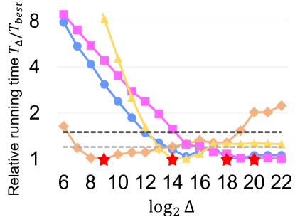
(a). Twitter (TW)	(b). Friendster (FT)	(c). WebGraph (WB)	(d). Road USA (USA)

Figure 1. $\Delta$-stepping relative running time with varying $\Delta$, including social networks (Twitter and Friendster), web graph (WebGraph), and road network (Road USA). A complete version with seven graphs is presented in Fig. 14. We use 96 cores (192 hyperthreads). We vary $\Delta$ and report the running time divided by the best running time across all $\Delta$ values. The best choice of $\Delta$ for each implementation is marked as a red star. We have the following interesting findings. (1). On the same graph, the best delta can be very different for different implementations (e.g., on Twitter, Julienne’s best $\Delta$ is $2^{12}$ times larger than Galois’s). The best value of delta for one algorithm can make another implementation much slower (e.g., Galois’s best $\Delta$ on Friendster makes all other implementations more than $4\times$ slower). The selection of $\Delta$ for one $\Delta$-Stepping implementation does not generalize to other $\Delta$-Stepping implementations. (2) For each implementation, the best choices of $\Delta$ vary a lot on different graphs ($2^{8}$ for GAPBS), although they have similar edge weight range and distribution. (3). On the same graph, the performance is very sensitive to the value of $\Delta$. Usually, $2$–$4\times$ off may lead to a 20% slowdown, and $4$–$8\times$ off may lead to a 50% slowdown. A badly-chosen parameter delta can largely affect the performance. (4). For the same implementation, on different graphs, the performance variance changing with $\Delta$ can be unstable. For example, Galois has very stable performance across $\Delta$ values on com-orkut (see Fig. 14) and Twitter, but is very unstable on other graphs. Thus, the stable performance on one graph does not guarantee that we can avoid searching the full parameter space for another graph.

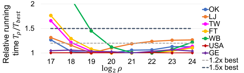
Figure 2. Relative running time of $\rho$-Stepping with varied $\rho$. We use 96 cores (192 hyperthreads). We vary $\rho$ and tested the average running time on 100 random sources, and divided by the time with the best $\rho$. We can see that: (1) the trends are pretty consistent among all graphs; (2) when $\rho$ is between $2^{20}$ to $2^{24}$, the performance is almost always within $1.2\times$ the best performance (except for two LJ’s data points); (3) the best choices of $\rho$ are within $2^{19}$ to $2^{22}$, although the graph sizes vary by almost three orders of magnitudes; and (4) If we pick $\rho$ to be $2^{21}$, all runtimes are within 10ms off from the best cases (numbers in Table 4).

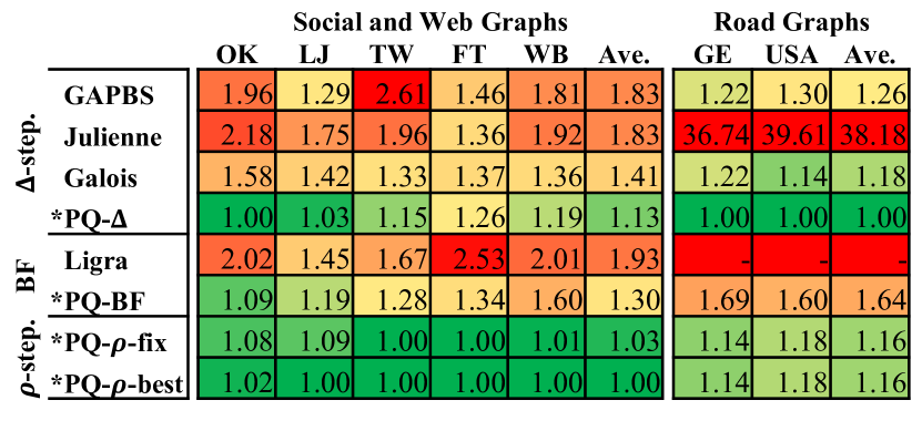
Figure 3. The heat map of the parallel running time relative to the fastest on each graph. We use 96 cores (192 hyperthreads). Each column is a graph instance. “Ave.” gives the average numbers over five social/web graphs and two road graphs, respectively. “*” denotes our implementations. PQ-$\rho$-fix means to use a fixed parameter $\rho$ across all graphs in $\rho$-Stepping, and PQ-$\rho$-best denotes the best running time using all values of $\rho$.

Our approach. The three previous research directions on parallel SSSP (practical implementations, theoretical bounds, parallel priority queues) are mostly studied independently. We aim to design parallel SSSP algorithms combining the advantages—as simple as those using parallel priority queues, achieving worst-case guarantees that match the existing bounds, and as fast as (or faster than) $\Delta$-Stepping in practice. Our key algorithmic insights include three components: a stepping algorithm framework, which abstracts general ideas in some existing parallel SSSP algorithms, an abstract data type (ADT) Lazy-Batched Priority Queue (LaB-PQ) with efficient implementations, which extracts the semantics of the priority queue needed by stepping algorithms, and two new stepping algorithms $\rho$-Stepping and $\Delta^{*}$-Stepping, which are efficient both in theory and practice.

Our stepping algorithm framework (Algorithm 1) abstracts the common idea in some existing “stepping” algorithms (e.g., Radius-Stepping (blelloch2016parallel, ) and $\Delta$-Stepping (meyer2003delta, )): in each step, the algorithm relaxes all vertices with tentative distances within a certain threshold, as a batch and in parallel. The two extreme cases are the two textbook algorithms: Dijkstra’s algorithm with batch size 1, and Bellman-Ford algorithm with batch size $n$. We formalize several algorithms in this framework (Tab. 2). Interestingly, some variants of parallel Dijkstra (bingmann2015bulk, ; zhou2019practical, ; alistarh2015spraylist, ) also use a similar high-level idea.

The proposed ADT LaB-PQ abstracts the priority queue needed by the stepping algorithms. It supports Update to commit an update to the data structure, which can be lazily batched and executed in parallel. It also supports Extract to return all records with keys within a certain threshold in parallel. The LaB-PQ is inspired by the recent work on batch-dynamic data structures  (shun2014phase, ; acar2019parallel, ; anderson2020work, ; tseng2019batch, ; Blelloch2016justjoin, ; sun2018pam, ), where multiple updates or queries are applied to the data structure in batches in parallel. One advantage of LaB-PQ is that we do not explicitly generate the batches, but do it lazily. On top of the ADT, all stepping algorithms can easily use LaB-PQ’s interface as a black box. Underneath it, we provide efficient data structures to support LaB-PQ. We show a theoretically efficient implementation of LaB-PQ based on the tournament tree (Sec. 4.2). It improves the cost bounds for existing parallel SSSP algorithms such as Radius-Stepping (blelloch2016parallel, ) and Shi-Spencer (Shi1999, ). In practice, we show simple implementations based on flat arrays, which makes our stepping algorithms outperform state-of-the-art software (zhang2020optimizing, ; dhulipala2017, ; nguyen2013lightweight, ; beamer2015gap, ).

Based on the stepping algorithm framework and LaB-PQ, we also propose a new parallel SSSP algorithm, referred to as $\rho$-Stepping, which is simple and efficient both in theory and in practice. The high-level idea of $\rho$-Stepping is to relax a fixed number of unsettled vertices with small tentative distances in each step. While a similar (but not the same) idea have been used in some parallel Dijkstra’s algorithms (bingmann2015bulk, ; zhou2019practical, ; alistarh2015spraylist, ), none of them have interesting bounds or practical performance comparable to $\Delta$-Stepping. In this paper, we formally analyze $\rho$-Stepping and show work and span bounds. $\rho$-Stepping achieves a better span bound than Radius-Stepping with a slightly higher work bound (Thm. 3.1). The work bound also applies to directed graphs (the bounds for Radius-Stepping only holds for undirected graphs). Practically, our $\rho$-Stepping is 1.3-2.6$\times$ faster than previous implementations on social and web graphs, and is competitive on road graphs (Fig. 3).

In addition to theoretical guarantees and practical performance, another advantage of $\rho$-Stepping is that, it needs no preprocessing (e.g., adding shortcuts in Radius-Stepping) or time-consuming parameter searching (e.g., finding best $\Delta$ in $\Delta$-Stepping). Our experiments (Fig. 2) show that, the best choice of $\rho$ is consistent and insensitive across the real-world graphs we tested.

Inspired by the stepping algorithms and LaB-PQ, we also show $\Delta^{*}$-Stepping, a variant of $\Delta$-Stepping, which is simple, has non-trivial worst-case bounds (Tab. 3), and fast in practice (Fig. 3).

Our Contributions. Combining our LaB-PQ with existing algorithms and our new algorithms, we achieve new bounds and efficient implementations for parallel SSSP. These results are due to the abstraction of stepping algorithm framework and LaB-PQ, which greatly simplifies algorithm design, analysis, and implementation.

In theory, we show new bounds for Radius-Stepping (blelloch2016parallel, ), Shi-Spencer (Shi1999, ), $\Delta^{*}$-Stepping, and $\rho$-Stepping. We note that, with no shortcuts or hopsets, it seems unlikely to show $o(n)$ worst-case span (consider a chain). However, tighter bounds can depend on certain graph parameters, which may exhibit a good property on real-world graphs. For example, although parallel Bellman-Ford has worst-case span of $\tilde{O}(n)$, a more precise bound is $\tilde{O}(d)$, where $d$ is the shortest-path tree depth. Indeed, on social networks with small $d$, parallel Bellman-Ford is reasonably fast (Table 4). To capture this, Blelloch et al. (blelloch2016parallel, ) proposed a graph invariant $(k,\rho)$-graph that indicates how “parallel” a graph is. Intuitively, a graph is a $(k,\rho)$-graph if every vertex reaches $\rho$ nearest vertices in $k$ hops. We extend this concept to analyze multiple stepping algorithms. Our experiments show that the real-world social or web graphs we tested are $(\log n,O(\sqrt{n}))$-graphs, and road graphs we tested are $(\sqrt{n},O(n))$-graphs (Fig. 9). Under our framework, the stepping algorithms share common subroutines in analyses, such as the extraction lemma (Lem. 5.1) and the distribution lemma (Lem. 5.2).

In practice, our framework and array-based LaB-PQ give unified implementations for Bellman-Ford, $\Delta^{*}$-Stepping and $\rho$-Stepping. Our implementations achieve the best performance on all graphs (see Fig. 3). On the social and web graphs, $\rho$-Stepping is 1.3-2.6$\times$ faster than existing implementations. On road graphs, our $\Delta^{*}$-Stepping is consistently the fastest and $\rho$-Stepping is competitive to previous ones. This indicates the effectiveness of our framework since all optimizations are easily applicable to all algorithms. We also provide an in-depth experimental study based on our framework, especially to understand the tradeoff between work and parallelism. We show how different stepping algorithms explore the frontier in steps (Figs. 9 and 9), the parameter space (Figs. 1 and 2), and eventually draw interesting conclusions in Fig. 9.

We summarize our contributions of this paper as follows.

• A stepping algorithm framework, which unifies multiple parallel SSSP algorithms.

• A new ADT LaB-PQ and two implementations, which are used in our analysis and implementations, respectively.

• A new parallel SSSP algorithm $\rho$-Stepping, which is preprocessing-free, simple and efficient both in theory and in practice.

• A new variant of $\Delta$-Stepping ($\Delta^{*}$-Stepping), which is simple, with theoretical guarantee, and fast in practice.

• New analyses for stepping algorithms based on $(k,\rho)$-graph, which include parameterized work and span bounds for $\rho$-Stepping (Thm. 3.1) and $\Delta^{*}$-Stepping (Thm. 5.6), and improved work bounds for Radius-Stepping (Col. 5.4) and Shi-Spencer (Col. 5.5).

• Efficient parallel implementations of Bellman-Ford, $\Delta^{*}$-Stepping and $\rho$-Stepping, which outperform existing ones (Tab. 4).

• In-depth experimental study of parallel SSSP algorithms.

2. Preliminaries

Computational Model. This paper uses the work-0pt model for fork-join parallelism with binary forking to analyze parallel algorithms (CLRS, ; blelloch2020optimal, ), which is used in many recent papers on parallel algorithms (agrawal2014batching, ; Acar02, ; blelloch2010low, ; BCGRCK08, ; BG04, ; Blelloch1998, ; blelloch1999pipelining, ; BlellochFiGi11, ; BST12, ; Cole17, ; CRSB13, ; BBFGGMS16, ; dinh2016extending, ; chowdhury2017provably, ; blelloch2018geometry, ; dhulipala2020semi, ; BBFGGMS18, ; Dhulipala2018, ; blelloch2020randomized, ; gu2021parallel, ).

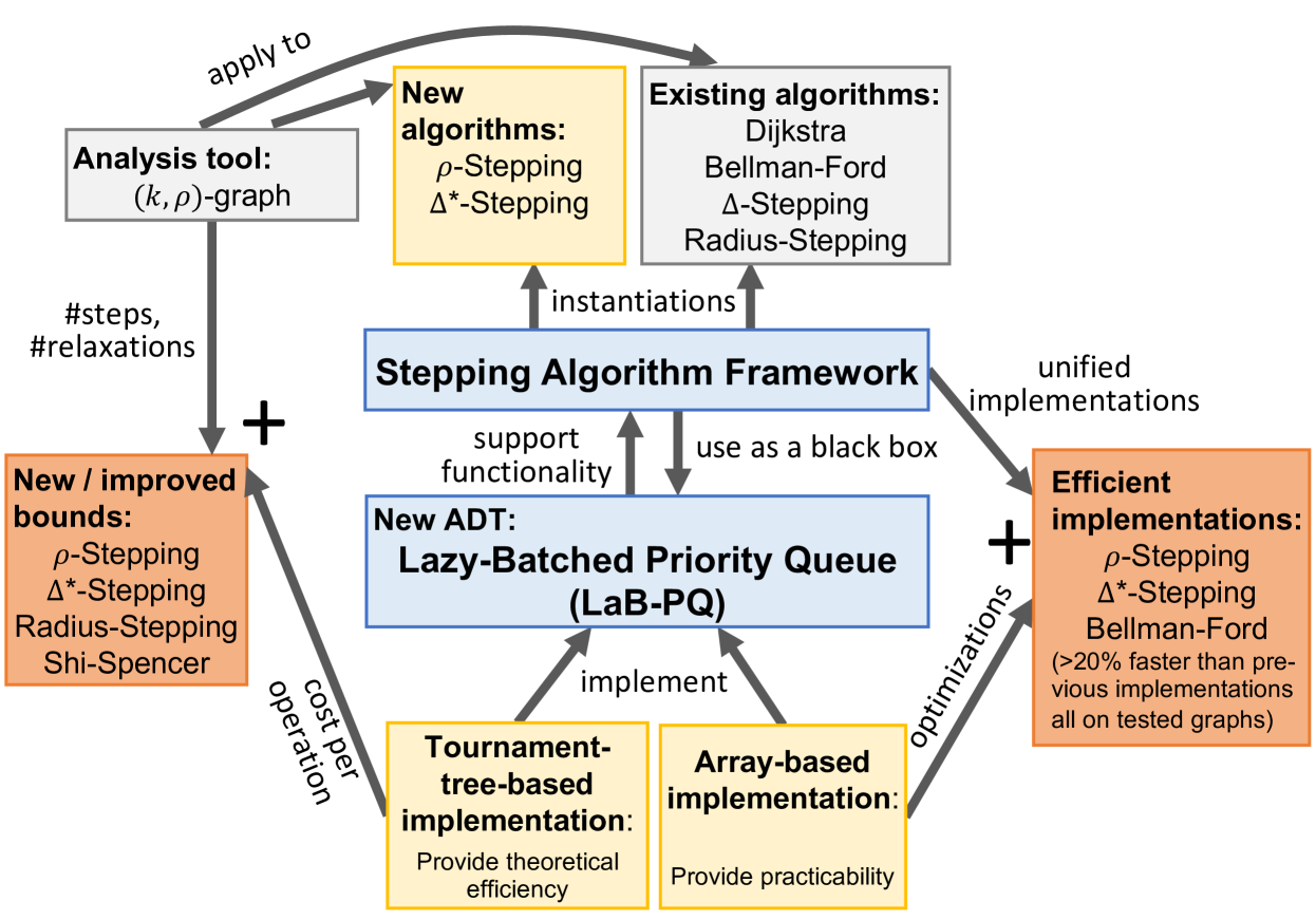
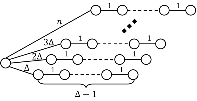
Figure 4. An overview of all components in this paper and how they are put together. The two blue boxes are the abstractions, one for the algorithms and one as an ADT. The yellow boxes are new algorithms and data structures in this paper. Grey boxes are existing results we use in this paper. The two orange boxes are the outcomes of all the techniques, including new work and span bounds for parallel SSSP, and faster implementations as compared to state-of-the-art software.

Figure 5. An example that incurs $O(n)$ span for $\Delta$-Stepping on a graph with $\Theta(\Delta)$ shortest path tree depth. On this graph, $\Delta$-Stepping algorithm needs to run $O(n/\Delta)$ rounds (steps) since the longest distance is $O(n)$. Within each step, we need to run $O(\Delta)$ Bellman-Ford substeps, which will settle the chains respectively. The $\Delta^{*}$-Stepping variant proposed in this paper only requires $O(n/\Delta+\Delta)$ rounds (steps) for this graph instance.

We assume a set of threads that share a common memory. Each thread supports standard RAM instructions, and a fork instruction that forks two new child threads. When a thread performs a fork, the two child threads all start by running the next instruction, and the original thread is suspended until all children terminate. A computation starts with a single root thread and finishes when that root thread finishes. An algorithm’s work is the total number of instructions and the span (depth) is the length of the longest sequence of dependent instructions in the computation. We can execute the computation using a randomized work-stealing scheduler in practice. We assume unit-cost atomic operation WriteMin$(p,\mathit{v})$, which reads the memory location pointed to by $p$, and write value $v$ to it if $v$ is smaller than the current value. We also use atomic operation TestAndSet$(p)$, which reads and attempts to set the boolean value pointed to by $p$ to true. It returns true if successful and false otherwise.

Graph Notations. We consider a weighted graph $G=(V,E,w)$. WLOG, we assume $G$ is a connected, simple graph, with minimum edge weight $\min_{e\in E}w(e)=1$, and no parallel edges) We use $L=\max_{e\in E}w(e)$. For $v\in V$, define $N(v)=\{u\,|\,(v,u)\in E\}$ as the neighbor set of $v$. We use $d(u,v)$ as the shortest-path distance in $G$ between two vertices $u$ and $v$. A shortest-path tree rooted at vertex $u$ is a spanning tree $T$ of $G$ such that the path distance in $T$ from $u$ to any other $v\in V$ is $d(u,v)$.

$(k,\rho)$-graph. We use the concept of $(k,\rho)$-graph in (blelloch2016parallel, ) to analyze stepping algorithms. $(k,\rho)$-graph is a graph invariant highly related to the analysis of parallel SSSP algorithms. Intuitively, a graph is a $(k,\rho)$-graph if any vertex can reach its $\rho$ nearest neighbors in $k$ hops. More formally, we define the hop distance $\hat{d}(u,v)$ from a vertex $v$ to $u$ as the number of edges on the shortest (weighted) path from $v$ to $u$ using the fewest edges. Let $r_{\rho}(v)$ be the $\rho$-th closest distance from $v$, and $\bar{r}_{k}(v)$ the shortest distance from $v$ to another vertex more than $k$-hops away.

Definition 1 ( $(k,\rho)$-graph (blelloch2016parallel, ) ).

We say a graph $G=(V,E,w)$ is a $(k,\rho)$-graph if for all $v\in V$, $r_{\rho}(v)\leq\bar{r}_{k}(v)$.

For a given graph $G=(V,E)$, we denote $k^{G}_{\rho}$ to be the smallest value for $k$ to make $G$ a $(k,\rho)$-graph. With clear context, we omit the superscription. $k_{n}$ is the shortest-path tree depth.

Others. We use $\log n$ as a short form of $1+\log_{2}(n+1)$. We say $O(f(n))$ with high probability (whp) to indicate $O(cf(n))$ with probability at least $1-n^{-c}$ for $c\geq 1$, where $n$ is the input size.

3. Frameworks

3.1. The LaB-PQ Abstraction

An abstract data type Lazy-Batched Priority Queue, or LaB-PQ, denoted as $\mathbb{PQ}$, maintains a universe of records $({\mathit{id}}{},k)$, where ${\mathit{id}}{}\in I$ is the unique identifier for this record and $k\in K$ is the key. In some applications, each record also has a value $v\in V$. In this paper, if not specified, we assume an empty value type for simplicity. In many applications, the identifier type $I$ is the natural number set $\mathbb{N}$. In all SSSP algorithms in this paper, the identifiers are vertex labels from 1 to $n$. The total ordering of all keys is determined by a comparison function $<_{K}:K\times K\mapsto\mathit{Bool}{}$. A LaB-PQ $Q\in\mathbb{PQ}$ is associated with a mapping function $\delta_{Q}:I\mapsto K$, which maps an identifier to its corresponding key (or key-value) that can change dynamically over time. With clear context, we omit the subscription $Q$, and use $\delta[{\mathit{id}}]$ to denote the mapping from ${\mathit{id}}$ to key. In the SSSP algorithms of this paper, this mapping function maps each vertex label to its (tentative) distance. In our implementation, this mapping function is passed to LaB-PQ by a pointer to the tentative distance array. More formally, a LaB-PQ $\mathbb{PQ}$ is parameterized on the following:

$\bm{I}$	Unique identifier type
$\bm{K}$	Key type
$\bm{V}$	(Optional) Value type
$\bm{<_{K}}:K\times K\mapsto\mathit{Bool}$	Comparison function on $K$
$\bm{\delta_{Q}}:I\mapsto K\times V$	A mapping from an id to its key (or key-value)

A LaB-PQ maintains a subset of identifiers in the universe. It can extract records with (relatively) small keys in parallel based on $\delta[\cdot]$. The interface of the LaB-PQ includes two functions: Update and Extract (see Table 1).We note that these two functions are sufficient for SSSP application. We discuss more functionalities of LaB-PQ in Appendix D.

Update$({\mathit{id}})$ function commits an update to $Q$ regarding the record with identifier ${\mathit{id}}$. It “notifies” $Q$ that the new key for this record is now in $\delta[{\mathit{id}}]$. If ${\mathit{id}}$ is not in $Q$ yet, Update inserts it to $Q$. Multiple Update can be executed concurrently. We note that the change of the record is embodied in the change of $\delta[{\mathit{id}}]$, and thus the data structure only needs to know the record’s ${\mathit{id}}$ to address the modification. An important observation is that, we do not have to modify $Q$ immediately, but can execute them lazily. These changes make no difference to any other operations on $Q$ before the next Extract. Compared to the classic “batch-dynamic” setting, our interface avoids explicitly generating the batch, which simplifies the algorithm and improves performance.

Extract$(\theta)$ returns all identifiers in $Q$ with key $\leq\theta$, and then deletes them from $Q$. Note that the result of Extract reflects all previous modifications to $Q$, including Update functions and deletions from the previous Extract. It then extracts the corresponding records based on the latest view of $Q$. An Extract function cannot be executed concurrently with other functions (Update or another Extract). This is required for LaB-PQ’s correctness.

Augmenting LaB-PQ. In some applications, we need a “sum” (the augmented value of type $A$) of all records (keys and possible values) in the LaB-PQ . We refer to this as $Q.{\mbox{\sc{Reduce}}}()$. This function first map each record in $Q$ to a value of type $A$, and use a binary commutative and associative operator $\oplus$ ($(A,\oplus)$ is a commutative monoid) to compute abstract sum of all records in $Q$ using $\oplus$.

$Q.{\mbox{\sc{Update}}}({\mathit{id}})$: $\mathbb{PQ}\times I\mapsto\Box$	Modify the record with identifier ${\mathit{id}}$ in $Q$ to $\delta[{\mathit{id}}]$. If ${\mathit{id}}\notin Q$, first add it to $Q$.
$s=Q.$Extract$(\theta)$: $\mathbb{PQ}\times K\mapsto\mathit{seq}$	Return identifiers in $Q$ with keys no more than $\theta$ and delete them from $Q$.

Table 1. Interface of LaB-PQ.

3.2. The Stepping-Algorithm Framework

Algorithm	ExtDist	FinishCheck	Work	Span
Dijkstra (dijkstra1959, )	$\displaystyle\theta\leftarrow\min_{v\in Q}(\delta[v])$	-	$\tilde{O}(m)$	$\tilde{O}(n)$
Bellman-Ford (bellman1958routing, ; ford1956network, )	$\theta\leftarrow+\infty$	-	$\tilde{O}(k_{n}m)$	$\tilde{O}(k_{n})$
$\Delta$-Stepping (meyer2003delta, )	$\theta\leftarrow i\Delta$	if no new $\delta[v]<i\Delta$, $i\leftarrow i+1$	-	-
$\Delta^{*}$-Stepping (new)	$\theta\leftarrow i\Delta$	-	$\tilde{O}\mathopen{}\mathclose{{}\left(k_{n}m}\right)$	$\tilde{O}\mathopen{}\mathclose{{}\left(\frac{k_{n}(\Delta+L)}{\Delta}}\right)$
Radius-Stepping (blelloch2016parallel, )	$\displaystyle\theta\leftarrow\min_{v\in Q}(\delta[v]+r_{\rho}(v))$	if there exists $\delta[v]<\theta$, do not recompute ExtDist	$\tilde{O}(k_{\rho}m)$	$\tilde{O}\mathopen{}\mathclose{{}\left(\frac{k_{\rho}n}{\rho}\cdot\log{L}}\right)$
$\rho$-Stepping (new)	$\theta\leftarrow$ $\rho$-th smallest $\delta[v]$ in $Q$	-	$\tilde{O}(k_{n}m)$	$\tilde{O}\mathopen{}\mathclose{{}\left(\frac{k_{\rho}n}{\rho}}\right)$ (undirected)

Table 2. SSSP Algorithms in the stepping algorithm framework, their ExtDist and FinishCheck, and the work and span bounds based on the LaB-PQ implementation in Sec. 4. Here $L$ is the longest edge in the graph (assuming the shortest has length 1). $\rho$, $k_{\rho}$ and $k_{n}$ are related to $(k,\rho)$-graph defined in Sec. 2. $\tilde{O}()$ omits $\log n$ and lower-order terms for simplicity, and the full bounds are shown in Tab. 3.

Input: A graph $G=(V,E,w)$ and a source node $s$.

Output: The graph distances $d(\cdot)$ from $s$.

1 $\delta[\cdot]\leftarrow+\infty$, associate $\delta$ to a LaB-PQ $Q$

2 $\delta[s]\leftarrow 0$, $Q.{\mbox{\sc{Update}}}{}(s)$

3 while $|Q|>0$ do

4       ParallelForEach $u\in Q.{\mbox{\sc{Extract}}}({\mbox{\sc{ExtDist}}})$ do

5             ParallelForEach $v\in N(u)$ do

6                   if ${\mbox{\sc{WriteMin}}}(\delta[v],\delta[u]+w(u,v))$  then

7                         $Q.{\mbox{\sc{Update}}}{}(v)$

8      Execute FinishCheck

9return $\delta[\cdot]$

[.15em]

Algorithm 1 The Stepping Algorithm Framework.

On top of the LaB-PQ interface, we also propose a simple stepping algorithm framework, in order to reveal the internal connection of the existing SSSP algorithms. Recall the two sequential textbook algorithms, Dijkstra’s algorithm (dijkstra1959, ) and Bellman-Ford algorithm (bellman1958routing, ; ford1956network, ). Dijkstra only visits one vertex at a time and thus is work-efficient, but it is inherently sequential. Bellman-Ford visits all vertices in a step so it requires redundant work, but can be easily parallelized. Many parallel SSSP algorithms integrate the idea in both algorithms, and visit a subset of unsettled vertices close to the source node. Hence, they require less work than Bellman-Ford, and have better parallelism than Dijkstra. These algorithms are referred to as stepping algorithms (e.g., $\Delta$-Stepping and Radius-Stepping) since they process a batch of vertices in a step. This is captured by LaB-PQ in the stepping algorithm framework.

We present this stepping algorithm framework in Algorithm 1. This framework requires two user-defined functions, ExtDist and FinishCheck. Many SSSP algorithms can be instantiated by plugging in different ExtDist and FinishCheck functions (see Tab. 2). Algorithm 1 starts with associate the distance array $\delta$ to a LaB-PQ $Q$. It then runs in steps. In each step, we process vertices with distances within a threshold $\theta$, which is computed by ExtDist and used as the parameter of Extract. The extracted vertices will relax their neighbors using WriteMin (Algorithm 1). If successful, we call Update on the corresponding neighbor. Some algorithms (e.g., $\Delta$-Stepping) contain substeps in each step. This is captured by FinishCheck—if the condition is not true, the threshold $\theta$ will not be recomputed. We say a vertex $v$ is settled the last time it is extracted from the LaB-PQ and relaxes all its neighbors (and thus its distance does not change thereafter). We define the frontier as all vertices in $Q$, which are those waiting to be explored to relax their neighbors.

The stepping algorithm framework applies to various algorithms as shown in Tab. 2. We now briefly introduce them.

Dijkstra and Bellman-Ford. Dijkstra’s algorithm visits and settles the vertex with the closest distance in the frontier. By setting $\theta$ as $\min_{v\in Q}(\delta[v])$, Algorithm 1 works the same as Dijkstra’s algorithm, with the exception that multiple vertices with the same distances will be processed together, which does not affect correctness and efficiency. Finding the closest vertex can be supported using ${\mbox{\sc{Reduce}}}()$ and taking $\min$ on keys. Bellman-Ford visits all vertices in the frontier in each step, so we set $\theta$ as infinity, and in each step Algorithm 1 relaxes the neighbors of all vertices in $Q$.

$\Delta$-Stepping. As a hybrid of Dijkstra and Bellman-Ford, $\Delta$-Stepping visits and settles all the vertices with shortest-path distances between $i\Delta$ and $(i+1)\Delta$ in step $i$. Within each step, the algorithm runs Bellman-Ford as substeps. Hence we can set $\theta$ to $i\Delta$, and use FinishCheck to check if any newly relaxed vertex still has distance within $i\Delta$. If not, we increment $i$ and proceed to the next step.

$\Delta^{*}$-Stepping. We note that FinishCheck is not necessary for $\Delta$-Stepping, just like other stepping algorithms. In fact, all existing implementations (zhang2020optimizing, ; nguyen2013lightweight, ; beamer2015gap, ; dhulipala2017, ) relaxed FinishCheck in different ways. In this paper, we show that removing FinishCheck in $\Delta$-Stepping (referred to as $\Delta^{*}$-Stepping) can lead to better bounds (Thm. 5.6) and good practical performance (Sec. 7).

Radius-Stepping. In Radius-Stepping, we precompute $r_{\rho}(v)$, the distance from each vertex $v$ to the $\rho$-th closest vertex, for all vertices. Then in each step, Radius-Stepping sets the threshold $\theta$ as $\min_{v\in Q}(\delta[v]+r_{\rho}(v))$, and then uses Bellman-Ford as substeps to compute the distances for vertices no more than the threshold. FinishCheck is needed by the theoretical analysis, which bounds the number of total substeps to be $O({(k_{\rho}n/\rho)}\cdot\log{\rho L})$.

To implement Radius-Stepping in our framework, we need an augmented LaB-PQ. We set $r_{\rho}(u)$ of a vertex $u$ as the value of each record. We map each record to $k+v$ for a record with key $k$ (distance) and value $v$ (vertex radius), and set the operator $\oplus$ as $\min$. The threshold in Extract is $\theta=\min_{v\in Q}(\delta[v]+r_{\rho}(v))$, computed by $Q.{\mbox{\sc{Reduce}}}()$. In Sec. 4, we show that maintaining the augmented values does not affect the asymptotical cost bounds.

$\rho$-Stepping. In this paper, we propose a new algorithm $\rho$-Stepping in the stepping algorithm framework. $\rho$-Stepping extracts the $\rho$ nearest vertices in the frontier, and relaxes their neighbors. The threshold $\theta$ is the $\rho$-th smallest element in $Q$. We overload the notation of $\rho$ from Radius-Stepping because they share high-level similarities in the theoretical analysis. The only step for $\rho$-Stepping in addition to the stepping algorithm framework is finding the $\rho$-th closest distance among all vertices in the frontier (the ExtDist). In our implementation, we simply use a sampling scheme that randomly pick $s=O(n/\rho+\log n)$ elements, sort them and pick the $(\rho s/n)$-th one. More details on how to find the $\rho$-th element is in Appendix B, and an efficient implementation is in Sec. 6.

Picking the a subset of vertices with closest distances and relaxing their neighbors is not a groundbreaking idea, and has been used in the literature (e.g., (bingmann2015bulk, ; zhou2019practical, ; alistarh2015spraylist, )). However, the extracting process in previous work is either sequential or concurrent, so none of the existing algorithms support non-trivial work and span bounds, or practical efficiency as compared to $\Delta$-Stepping. In this paper, we argue that this simple solution can achieve both theoretical and practical efficiency. Theoretically, we show that:

Theorem 3.1 (Cost for $\rho$-Stepping).

On a $(k_{\rho},\rho)$-graph $G$, the $\rho$-Stepping algorithm has in $O\mathopen{}\mathclose{{}\left({k_{n}m}\log\frac{n^{2}}{m\rho}}\right)$ work and $O\mathopen{}\mathclose{{}\left(\frac{k_{n}n\log n}{\rho}}\right)$ span. If $G$ is undirected, the span is $O\mathopen{}\mathclose{{}\left(\frac{k_{\rho}n\log n}{\rho}}\right)$.

We will first show implementations of LaB-PQ and the cost, and then formally prove this result in Sec. 5.4. $\rho$-Stepping also has good practical performance, which is shown in Sec. 7.

4. LaB-PQ Implementation

We now discuss how to efficiently support LaB-PQ in Algorithm 1. We present two data structures for LaB-PQ with the goal of theoretical and practical efficiency, respectively. The obliviousness for data structures from the algorithm’s perspective is an advantage of the LaB-PQ ADT.

In our analysis, we define a batch of modifications as all Update operations between two invocations of Extract functions. The modification work on a batch $B$ is all work paid to Update all records in $B$, as well as any later work (done by a later Extract) to actually apply the updates. We define a batch of extraction as all records returned by an Extract function. The extraction work on a batch $B$ is all work paid to output the batch from the Extract function, as well as any later work (done by the next Extract) to actually remove them from $Q$.

4.1. Related Work

Early PRAM and BSP algorithms had explored parallel priority queues in a variety of approaches (brodal1998parallel, ; chen1994fast, ; das1996optimal, ; pinotti1991parallel, ; ranade1994parallelism, ; crupi1996parallel, ; baumker1996realistic, ), and heavily rely on synchronization-based techniques such as pipelining. These algorithms do not have better bounds than recent batch-dynamic search trees (Blelloch2016justjoin, ; sun2018pam, ; blelloch2020optimal, ; sun2019implementing, ; sun2019parallel, ) when mapping to the fork-join model. Other previous papers considered the concurrent, external-memory, and other settings (alistarh2015spraylist, ; sundell2005fast, ; linden2013skiplist, ; shavit2000skiplist, ; liu2012lock, ; henzinger2013quantitative, ; zhou2019practical, ; calciu2014adaptive, ; bingmann2015bulk, ; sanders2019sequential, ; sanders1998randomized, ; sanders2000fast, ). These data structures also do not have better bounds than batch-dynamic search trees since they do not focus on optimizing work or span. However, existing batch-dynamic search trees or other data structures (e.g., skiplists) maintaining the total ordering of the records, incur an $\Omega(\log(n))$ work lower bound per record update (more details are in the full paper). Our key observation is that maintaining total ordering, which incurs overhead both theoretically and practically, is not necessary for a parallel priority queue.

To the best of our knowledge, the only parallel data structure that has similar bounds to our new data structure is the batch-dynamic binary heap (wang2020parallel, ). However, it has a few disadvantages: it does not support efficient batch-extract, is very complicated (no implementation available), and the span is suboptimal ($O(\log^{2}n)$ in the binary fork-join model). Our new tournament-tree based LaB-PQ supports full features in the LaB-PQ, has $O(\log n)$ span, and is arguably much simpler.

4.2. Tournament-Tree-Based Implementation

We start with introducing the tournament tree (aka. winner tree). It is a complete binary tree with $n$ external nodes (leaves) and $n-1$ interior nodes. A tournament tree stores the records in the leaves. In our use case, we only need to store the record ${\mathit{id}}$ in the leaves using the LaB-PQ interface. Each interior node stores $k\in K$ ($K$ is in key type for the records) that takes the smaller key (defined by $<_{K}$) from its children. Fig. 6(a) illustrates a tournament tree when keys are integers and $<_{K}$ is $<_{\mathbb{Z}}$.

Figure 6. A tournament tree. Square leaf nodes store the records and round interior nodes keep the smallest key in their subtrees. (a) is a tournament tree containing 6 records $3,8,4,6,1$ and $5$. (b) shows an update on a batch of $3,8$ and $6$. The shaded nodes are marked as renewed.

We now discuss how to use a tournament tree to implement LaB-PQ. We will use $t.{\mbox{\emph{left}}}$, $t.{\mbox{\emph{right}}}$ and $t.{\mbox{\emph{parent}}}$ to denote the left child, right child and parent of a node $t$. For simplicity, we assume the universe of the records has a fixed size $n$ (for SSSP $n=|V|$), and the tournament tree has $n$ leaf nodes each with a boolean flag inQ indicating if this record is in (has been inserted to) the LaB-PQ $Q$. We note that this is sufficient for the SSSP algorithms. The dynamic version (where the size of the tournament tree changes with the size of LaB-PQ) will be described in the full paper.

1 Maintains A tournament tree $T$ with $n$ leaf nodes each corresponding to a record.

2Function ${\mbox{\sc{Mark}}}($record id ${\mathit{id}}$, boolean flag ${\mbox{\emph{newflag}}})$

3       Let $t$ be the tree leaf corresponding to id

4       $t.\mathit{inQ}\leftarrow{\mbox{\emph{newflag}}}$

5       while $t\neq T.root$ and TestAndSet$(t.{\mbox{\emph{parent}}}.{\mbox{\emph{renew}}})$ do

6             $t\leftarrow t.{\mbox{\emph{parent}}}$

7 Function ${\mbox{\sc{Sync}}}($node $t)\to k\in K$

8       if $t$ is leaf then

9             if $t.{\mbox{\emph{inQ}}}$ then return $\delta[t.id]$

10             else return $+\infty$

11            

12      if $t.{\mbox{\emph{renew}}}=0$ then return $t.k$

13      $t.{\mbox{\emph{renew}}}\leftarrow 0$

14       In Parallel:

15             ${\mbox{\emph{leftKey}}}\leftarrow{\mbox{\sc{Sync}}}(t.{\mbox{\emph{left}}})$

16             ${\mbox{\emph{rightKey}}}\leftarrow{\mbox{\sc{Sync}}}(t.{\mbox{\emph{right}}})$

17      return $t.k\leftarrow\min({\mbox{\emph{leftKey}}},{\mbox{\emph{rightKey}}}$)

18 Function ${\mbox{\sc{ExtractFrom}}}(\text{threshold }\theta\text{, node }t)\to{\mbox{\emph{seq}}}$

19       if $t$ is a leaf then

20             if $(\delta[t.{\mathit{id}}]\leq\theta)$ then

                   ${\mbox{\sc{Mark}}}(t.{\mathit{id}},0)$

                    // Marked as not in Q

21                   return $\{t.{\mbox{\emph{id}}}\}$

22            else return $\{\}$

23            

24      if $\theta<t.k$ then return $\{\}$ // empty seq

25       In Parallel:

26             ${\mbox{\emph{leftseq}}}\leftarrow{\mbox{\sc{ExtractFrom}}}(\theta,t.{\mbox{\emph{left}}})$

27             ${\mbox{\emph{rightseq}}}\leftarrow{\mbox{\sc{ExtractFrom}}}(\theta,t.{\mbox{\emph{right}}})$

28      return ${\mbox{\emph{leftseq}}}+{\mbox{\emph{rightseq}}}$

29 Function ${\mbox{\sc{Extract}}}(\text{threshold }\theta$)

30       ${\mbox{\sc{Sync}}}(T.{\mbox{\emph{root}}})$

31       return ${\mbox{\sc{ExtractFrom}}}(\theta,T.{\mbox{\emph{root}}})$

32 Function ${\mbox{\sc{Update}}}({\mathit{id}}$)

33       ${\mbox{\sc{Mark}}}({\mathit{id}}{},1)$

34      

Algorithm 2 The Tournament-tree based LaB-PQ.

A tournament tree $T$ on $n$ records contains $2n-1$ nodes in total. The first $n-1$ nodes are interior nodes. For an interior node $t$, we use $t.k$ to denote the key stored in node $t$. To support the LaB-PQ interface, each interior node contains a bit flag renew indicating if any key in its subtree has been modified after the last update of $t.k$. This flag is initially set to 0 (false).

Constructing such a tree with given initial values simply takes linear work and $O(\log n)$ span using divide-and-conquer: construct both subtrees recursively in parallel, and update the root’s key based on the two children’s keys.

We next present the implementation of LaB-PQ’s interface using tournament tree. Due to page limit, we only show the pseudocode (Algorithm 2) and a high-level overview here. The analysis are given in the full paper. We first introduce a helper function Mark$({\mathit{id}}{},{\mathit{newflag}})$.

Mark$({\mathit{id}}{},{\mathit{newflag}})$ first sets the record ${\mathit{id}}$’s ${\mathit{inQ}}$ flag to be ${\mathit{newflag}}$—0 means the record should be deleted, and 1 means inserted. Whichever value ${\mathit{newflag}}$ is, this means the record of ${\mathit{id}}$ has been updated. Then, the algorithm marks the renew flags of the nodes on the tree path from the updated leaf to the root. This process is executed using TestAndSet. If the TestAndSet fails, we know that another Mark has marked the rest of the path, so the current Mark terminates immediately. An example is shown in Fig. 6(b). Updating the nodes’ keys is postponed to the next Extract function.

Update.  The Update algorithm simply calls Mark$({\mathit{id}}{},1)$.

Extract.  Extract first uses a function Sync to update the keys for all nodes with renew flag as 1. It then calls ExtractFrom to output all records with keys no more than $\theta$. Those output keys are also marked as deleted from $T$ (Algorithm 2).

The ${\mbox{\sc{Sync}}}{}(t)$ function recursively restores the keys in the interior nodes using a divide-and-conquer approach (Algorithm 2–2), and returns the key at the current node $t$. The return value of a leaf node is either the record’s key or infinity, depending on the $\mathit{inQ}$ flag. For an interior node, Sync will update the key to be the smaller one of its two children and return this key. After all interior tree nodes have been updated, we use ExtractFrom to acquire all records with keys no more than $\theta$. This step can be parallelized similarly using divide-and-conquer (Algorithm 2–2): we can traverse the left and right subtrees respectively and concatenate the two results. A subtree is skipped when the key at the subtree root (minimum key in the subtree) is larger than $\theta$. Note that if we want the output sequence in a consecutive array, we can traverse for two rounds—the first round computes the number of extracted records, and the second round writes them to the corresponding slots.

We can implement Reduce similarly. We keep a collective status $t.a\in A$ ($A$ is the augmented value type) for each interior node $t$, and it is updated in the Update function in Algorithm 2–2 similar to the update for $k$. We do not need to update $t.a$ for node $t$ if the subtree rooted at $t$ remains unchanged, which is captured by $t.{\mbox{\emph{renew}}}$.

Theorem 4.1.

Consider a tournament tree on a universe of $n$ records, implemented with algorithms in Algorithm 2. The modification work on a size-$b$ batch is $O\mathopen{}\mathclose{{}\left(b\log(n/b)}\right)$. The extraction work on a size-$b$ batch is $O\mathopen{}\mathclose{{}\left(b\log(n/b)}\right)$. The span of Extract and Update is $O(\log n)$.

To prove this theorem, we will use the following lemma.

Lemma 4.2.

Given $b$ invocations of Mark function in a batch, the total cost of these Mark functions is $O\mathopen{}\mathclose{{}\left(b\log\frac{n}{b}}\right)$. If there are $b$ invocations of Mark function in the last batch, the total cost of the Sync is $O\mathopen{}\mathclose{{}\left(b\log\frac{n}{b}}\right)$. If the ExtractFrom algorithm extracts $b$ (smallest) elements from tournament tree $T$, the total cost of ExtractFrom is $O\mathopen{}\mathclose{{}\left(b\log\frac{n}{b}}\right)$.

• We first show that, in a tournament tree, for a subset $X$ of tree leaves, if we denote $S(X)$ as the set of all ancestors of nodes in $X$, then $|S(X)|=O\mathopen{}\mathclose{{}\left(|X|\log\frac{n}{|X|}}\right)$. This has been shown on more general self-balanced binary trees (Blelloch2016justjoin, ; blelloch2018geometry, ), and just a simplified case suffices as tournament trees are complete binary trees.

  First, Mark modifies the flag renew for each tree path node all modified leaves to the root. Let $X$ be all tree leaves corresponding to the invocations Mark functions in this batch. Therefore $|X|=b$. By definition of $S(X)$, we know that only nodes in $X\cup S(X)$ are visited. Because of the test_and_set operation, a node $v\in S(X)$ recursively call Mark on its parent $u$ if and only if $v$ successfully set the renew mark of $u$. This means that for any interior node $u\in S(X)$, this can happen only once. Therefore, every node in $S(X)$ is visited by the Mark function at most once. This proves that the cost of all Mark functions $O\mathopen{}\mathclose{{}\left(b\log\frac{n}{b}}\right)$.

  For Sync, it restores all relevant interior tree nodes top-down. Let $X$ be all tree leaves corresponding to the invocations Mark functions in the last batch (so that they need to be addressed in this Sync). Therefore $|X|=b$. Note that the algorithm skips a subtree when the renew flag is false. Therefore, the total number of visited nodes must be a subset of all nodes in $X\cup S(X)$ and their children. Given that each node has at most two children, this number can also be asymptotically bounded by $|X\cup S(X)|$, which are those marked true in the renew flags. This gives the same bound as the total cost of Mark functions in a batch.

  For Extract, denote the leaves corresponding to all the output records as set $X$ of size $b$. Note that we skip a subtree if its key (minimum key in its subtree) is larger than $\theta$. This means that we visit an interior node only if at least one of its descendants will be included in the output batch. Therefore, all visited nodes are also $X\cup S(X)$ and all their children. For all visited leaves, Extract also calls Mark to set inQ flag to 0 (false). As proved above, the total cost of these Mark functions is $O\mathopen{}\mathclose{{}\left(b\log\frac{n}{b}}\right)$. Therefore, the total cost of ExtractFrom is also $O\mathopen{}\mathclose{{}\left(b\log\frac{n}{b}}\right)$ to extract a batch of size $b$. ∎

With Lem. 4.2 that shows the cost of each function in Algorithm 2, we can now formally prove Thm. 4.1.

• Recall that the modification work on a batch $B$ as all work paid to Update all records in $B$, as well as any later work (possibly done by a later Extract) to actually apply the updates, and the extraction work on a batch $B$ is all work paid to output the batch from the Extract function, as well as any later work (possibly done by the next Extract) to actually remove them from $Q$. In tournament tree, the modification work includes all Mark operations called by the Update functions in the batch, as well as later cost in the Sync operation to restore keys of all the relevant interior nodes. From Lem. 4.2, the total cost is $O(b\log(\frac{n}{b}))$ for a batch of size $B$. The extraction work on a batch $B$ includes the work done by ExtractFrom to get the output sequence, as well as to restore keys of all the relevant interior nodes in the next Sync.

  For both Extract and Update, the span is no more than the height of the tree, which is $O(\log n)$. ∎

4.3. Array-Based Implementation

Algorithm 2 uses a tree-based structure to provide tight work bounds for applying a batch of modifications or extractions. This is asymptotically better than batch-dynamic search trees (Blelloch2016justjoin, ; sun2018pam, ; blelloch2020optimal, ). However, in practice, maintaining a tree-based data structure can be expensive because of larger memory footprint and random access. Even though we can implement a tournament tree in a flat array (no pointers), it still requires extra storage for interior nodes and incurs frequent random accesses (following tree path). When the batch size $b$ approaches $n$ and $O(\log(n/b))$ becomes small, the theoretical advantage of tournament trees becomes insignificant, and is asymptotically the same as just loop over all records.

This is observed by the practitioners. Most (if not all) practical SSSP implementations just keep an array for all records without maintaining sophisticated structures. This is because parallel SSSP algorithms usually use a very large value of $b$ to get sufficient parallelism. To implement Update on an array, we can just set a flag to indicate a record is added to $Q$. For Extract, we loop over the entire array and pack all records with keys within $\theta$ in parallel, which takes linear work and $O(\log n)$ span. While efficiently implementing the array requires many subtle details (shown in Sec. 6), asymptotically, the following bound is easy to see.

Theorem 4.3.

The array-based LaB-PQ requires $O(b)$ modification work on a size-$b$ batch. The extraction work on a size-$b$ batch is $O(n)$. The span of Extract and Update is $O(\log n)$.

5. Analysis for Stepping Algorithms

Algorithm	Work		Span	Previous Best
	Tournament-tree-based	Array-based		Work	Span
Dijkstra (dijkstra1959, ; brodal1998parallel, )	$O\mathopen{}\mathclose{{}\left(m\log\frac{n^{2}}{m}}\right)$	$O(m+n^{2})$	$O(n\log n)$	$O(m\log n)$	same
Bellman-Ford (bellman1958routing, ; ford1956network, )	$O(k_{n}m)$	$O(k_{n}m)$	$O(k_{n}\log n)$	same	same
$\Delta^{*}$-Stepping	$O\mathopen{}\mathclose{{}\left(k_{n}m\log\frac{nL}{m\Delta}}\right)$	$O\mathopen{}\mathclose{{}\left(k_{n}m+\frac{k_{n}n(\Delta+L)}{\Delta}}\right)$	$O\mathopen{}\mathclose{{}\left(\mathopen{}\mathclose{{}\left(\frac{k_{n}(\Delta+L)}{\Delta}}\right)\log n}\right)$	-	-
Radius-Stepping† (blelloch2016parallel, )	$O\mathopen{}\mathclose{{}\left(k_{\rho}m\log\frac{n^{2}\log{\rho L}}{m\rho}}\right)$ (U)	$O\mathopen{}\mathclose{{}\left(k_{\rho}m+\frac{k_{\rho}n^{2}}{\rho}\cdot\log{\rho L}}\right){}$ (U)	$O\mathopen{}\mathclose{{}\left(\frac{k_{\rho}n}{\rho}\cdot\log{\rho L}\log n}\right)$ (U)	$O\mathopen{}\mathclose{{}\left(k_{\rho}m\log n}\right){}$ (U)	same
Shi-Spencer† (Shi1999, )	$O\mathopen{}\mathclose{{}\left((m+n\rho)\log\frac{n^{2}}{m+n\rho}}\right)$ (U)	$O\mathopen{}\mathclose{{}\left(m+n\rho+\frac{n^{2}}{\rho}}\right)$ (U)	$O\mathopen{}\mathclose{{}\left(\frac{n\log n}{\rho}}\right)$ (U)	$O\mathopen{}\mathclose{{}\left((m+n\rho)\log n}\right)$ (U)	same
$\rho$-Stepping	$O\mathopen{}\mathclose{{}\left(k_{n}m\log\frac{n^{2}}{m\rho}}\right)$	$O\mathopen{}\mathclose{{}\left(k_{n}m+\frac{n^{2}k_{\rho}}{\rho}}\right)$ (U)	$O\mathopen{}\mathclose{{}\left(\frac{k_{\rho}n\log n}{\rho}}\right)$ (U)	-	-
		$O\mathopen{}\mathclose{{}\left(k_{n}m+\frac{n^{2}k_{n}}{\rho}}\right)$	$O\mathopen{}\mathclose{{}\left(\frac{k_{n}n\log n}{\rho}}\right)$

Table 3. New work and span bounds for the stepping algorithms and comparison to previous results. (U) indicates the bound only works for undirected graphs. (-) indicates no non-trivial bound is known to the best of our knowledge. (same) indicates the previous bound matches the tournament-tree-based work or the span. All new work bounds for $\Delta^{*}$-Stepping, Radius-Stepping, Shi-Spencer, and $\rho$-Stepping are based on the distribution lemma (Lem. 5.2) and the LaB-PQ bounds. Radius-Stepping and Shi-Spencer (noted with ^†) require preprocessing.

With the stepping algorithm framework (Algorithm 1) and LaB-PQ’s implementation, we can now formally analyze the cost bounds for the stepping algorithms, which are summarized in Tab. 3. Our new bounds are parameterized by the definition of $(k,\rho)$-graph shown in (blelloch2016parallel, ). We first show some useful results for all stepping algorithms in Sec. 5.1, and use them to prove the results in Sec. 5.2. We later show the span for $\rho$-Stepping on undirected graphs in Sec. 5.3, and compare with existing algorithms in Sec. 5.4.

5.1. Useful Results for All Stepping Algorithms

We first show two useful lemmas for all stepping algorithms.

Lemma 5.1 (Number of extractions).

In a stepping algorithm, a vertex $v\in V$ will not be extracted from the priority queue (Algorithm 1 in Algorithm 1) more than $k_{n}$ times.

• Consider the shortest path $P=\{v_{0}=s,v_{1},v_{2},\ldots,v_{l}=v\}$ from the source $s$ to $v$ with fewest hops. Since we assume the edge weights are positive, we know that $d(s,v_{i})<d(s,v_{j})$ for $i<j$. Hence, whenever $v$ is extracted from the priority queue, the earliest unsettled vertex $v_{i}$ in $P$ must also be extracted and settled. This is because $v_{i-1}$ is already settled and have relaxed $v_{i}$ in previous rounds, and $d(s,v_{i})\leq d(s,v)$. Based on the definition of the $(k,\rho)$-graph, we have $l\leq k_{n}$, which proves the lemma. ∎

Lemma 5.2 (Distribution).

If a stepping algorithm has $S$ steps, and incurs $U$ updates (relaxations), the total work is $\displaystyle O\mathopen{}\mathclose{{}\left(U\log(nS/U)}\right)$ using tournament-tree-based LaB-PQ.

• The work of a stepping algorithm consists of modification work for relaxations (updates) and extraction work applied to the LaB-PQ. Each extracted vertex corresponds to a previous successful relaxation, and an update and an extraction have the same cost per vertex. Hence, we only need to analyze modification costs since extraction costs are asymptotically bounded.

  The $U$ updates are distributed in $S$ steps. Let $u_{i}$ be the number of relaxations applied in step $i$ ($\sum_{i}{u_{i}}=U$). The overall work across all steps is $W=O(\sum_{i}{u_{i}\log(n/u_{i})})$. Since $u_{i}\log(n/u_{i})$ is concave, $\sum_{i}{u_{i}\log(n/u_{i})}\leq S\cdot((\sum_{i}{u_{i}}/S)\log(n/(\sum_{i}{u_{i}}/S)))=U\log(nS/U)$, which proves the lemma. ∎

5.2. Cost Bounds for Stepping Algorithms

With Lem. 5.2 and 5.1 for the stepping algorithms and Thm. 4.1 and 4.3 for LaB-PQ’s cost, we can now show the cost bounds shown in Tab. 3 except for one given in Sec. 5.3.

Dijkstra’s algorithm has $O(n)$ steps and $O(m)$ relaxations, Lem. 5.2 gives $O(m\log(n^{2}/m))$ work which is essentially better than Brodal et al.’s algorithm (brodal1998parallel, ) (their span is also $O(n\log n)$ on the fork-join model). Bellman-Ford has $O(k_{n})$ steps and $O(k_{n}m)$ relaxations, so the work is $O(k_{n}m)$ and the span is $O(k_{n}\log n)$. The following theorem shows the number of steps for $\rho$-Stepping.

Theorem 5.3 (Number of steps for $\rho$-Stepping).

On a $(k_{\rho},\rho)$-graph, the $\rho$-Stepping algorithm finishes in $O\mathopen{}\mathclose{{}\left(k_{n}n/\rho}\right)$ steps.

• In $\rho$-Stepping, each step can either be a full-extract, where $|Q|\geq\rho$ so we extract $\rho$ vertices with closest tentative distances, or a partial-extract, where $|Q|<\rho$ so we extract all but fewer than $\rho$ vertices. There can be at most $O\mathopen{}\mathclose{{}\left(k_{n}n/\rho}\right)$ full-extracts, since Lem. 5.1 shows that each vertex can only be extracted for $k_{n}$ times. Given that we have $n$ vertices in total, there can be at most $O\mathopen{}\mathclose{{}\left(k_{n}n/\rho}\right)$ full-extracts. We now show that at most $k_{n}$ partial-extracts can occur. Similar to the analysis for Lem. 5.1, once a partial-extract occurs, at least one vertex on the shortest path $P$ from source $s$ to any vertex $v$ is settled. Based on the definition of the $(k,\rho)$-graph, we have $|P|\leq k_{n}$, so in total, at most $k_{n}$ partial-extracts can occur. Putting both parts together proves the theorem. ∎

Combining the result with Lem. 5.2 gives the work bound of $\rho$-Stepping in Tab. 3.

We now show that we can get better work bounds for Radius-Stepping using LaB-PQ. Radius-Stepping extracts all vertices with distance within $\min_{v\in Q}(\delta[v]+r_{\rho}(v))$ in each step. The original papers uses a search tree to support this operation. We note that our LaB-PQ fully captures the need in Radius-Stepping. By replacing the search tree with our tournament tree and plugging in the numbers of relaxations and steps, we get the following results.

Corollary 5.4.

Radius-Stepping (blelloch2016parallel, ) uses $O\mathopen{}\mathclose{{}\left(k_{\rho}m\log\frac{n^{2}\log{\rho L}}{m\rho}}\right)$ work and $O\mathopen{}\mathclose{{}\left(\frac{k_{\rho}n}{\rho}\cdot\log{\rho L}\log n}\right)$ span, with $O(m\log n+n\rho^{2})$ work and $O(\rho\log\rho+\log n)$ span for preprocessing.

We can also improve another parallel SSSP algorithm Shi-Spencer (Shi1999, ) by replacing their original search-tree-based priority queue with our tournament tree (more details in Appendix C).

Corollary 5.5.

Shi-Spencer algorithm (Shi1999, ) can be computed using $O\mathopen{}\mathclose{{}\left((m+n\rho)\log\frac{n^{2}}{m+n\rho}}\right)$ work and $O\mathopen{}\mathclose{{}\left(\frac{n\log n}{\rho}}\right)$ span, with $O(m+n\rho^{2}\log n\log\rho)$ work and $O(\log n\log\rho)$ span for preprocessing.

We also derive the bounds for $\rho$-Stepping on directed graphs in Thm. 3.1, and give the formal analysis for $\Delta^{*}$-Stepping:

Theorem 5.6.

$\Delta^{*}$-Stepping uses $O\mathopen{}\mathclose{{}\left(\frac{k_{n}(\Delta+L)}{\Delta}}\right)$ steps, and thus has $O\mathopen{}\mathclose{{}\left(k_{n}m\log\frac{nL}{m\Delta}}\right)$ work and $O\mathopen{}\mathclose{{}\left(\frac{k_{n}(\Delta+L)}{\Delta}\log n}\right)$ span based on LaB-PQ.

• We first show the number of steps in $\Delta^{*}$-Stepping. The farthest vertices in the shortest-path tree has distance no more than $k_{n}L$ where $L$ is the largest edge weight. After $\lceil k_{n}L/\Delta\rceil$ steps, all vertices are included in the threshold, so the algorithm will finish in no more than another $k_{n}$ steps (the number of steps of Bellman-Ford). Hence, in total, $\Delta^{*}$-Stepping uses $S=O\mathopen{}\mathclose{{}\left(\frac{k_{n}(\Delta+L)}{\Delta}}\right)$ steps.

  Based on Lem. 5.1, we know the number of total relaxations are upper bounded $U=k_{n}m$. We can now use Lem. 5.2 to get the work bound:

  $$O\mathopen{}\mathclose{{}\left(U\log\frac{nS}{U}}\right)=O\mathopen{}\mathclose{{}\left(k_{n}m\log\frac{nk_{n}(\Delta+L)}{k_{n}m\Delta}}\right)=O\mathopen{}\mathclose{{}\left(k_{n}m\log\frac{n(\Delta+L)}{m\Delta}}\right)$$

  Note that since $m\geq n$, $\frac{n(\Delta+L)}{m\Delta}$ makes a difference only when $L>\Delta$. Hence, the work bound can be simplified as $O\mathopen{}\mathclose{{}\left(k_{n}m\log\frac{nL}{m\Delta}}\right)$. ∎

We note that for the original $\Delta$-Stepping, such bounds do not hold. An additional factor of $k_{n}$ will be introduced if we need to settle down all vertices in each step, as shown in Fig. 5.

5.3. Number of Steps for Undirected Graphs

We can show tighter span bounds for $\rho$-Stepping on undirected graphs, which is inspired by existing results including Radius-Stepping (blelloch2016parallel, ) and Shi-Spencer’s algorithm (Shi1999, ). We first give the main theorem for this section.

Theorem 5.7 (Number of steps, Undirected).

On an undirected $(k_{\rho},\rho)$-graph, the $\rho$-Stepping algorithm finishes in $O\mathopen{}\mathclose{{}\left(k_{\rho}n/\rho}\right)$ steps.

In real-world graphs, we usually have $k_{\rho}\ll\rho$ for large $\rho$. Hence, by picking a large $\rho$, say $n/\log n$, $\rho$-Stepping only requires a small number of rounds and provides ample parallelism. As a comparison, Radius-Stepping requires $O\mathopen{}\mathclose{{}\left(\frac{k_{\rho}n}{\rho}\log\rho L}\right)$ steps, a factor of $O(\log\rho L)$ more for the worst-case guarantee.

Our proof sketch is as follows. We will show that after step $(2k_{\rho}+3)t$ for $t\geq 1$, $\rho$-Stepping will successfully settle at least the closest $t\rho$ vertices from $s$ and relax their neighbors. We will show this by induction. We note that the base case trivially holds when $t=1$, since $s$ can reach $\rho$ closest vertices in $k$ hops. Assume this is true for $t$, we will show that this is also true for $t+1$.

We start with some notations. Let $\mathcal{N}_{\rho}(u)$ be the set of $\rho$-nearest vertices from vertex $u$. For simplicity, let $\mathcal{T}_{\rho}=\mathcal{N}_{\rho}(s)$ where $s$ is the source vertex. The inductive hypothesis assumes that vertices in $\mathcal{T}_{t\rho}$ are settled. We now show that within the next $2k_{\rho}+2$ steps, all vertices in $\mathcal{T}_{(t+1)\rho}\setminus\mathcal{T}_{t\rho}$ are settled (updated to the exact distance).

Let $v\in\mathcal{T}_{(t+1)\rho}\setminus\mathcal{T}_{t\rho}$ and $P=\{s=v_{0},v_{1},v_{2},\dots,v_{l}=v\}$ be a the shortest path from $s$ to $v$ with the fewest hops. Assume all vertices $v_{0}$ through $v_{i}$ are in $\mathcal{T}_{t\rho}$, and beyond $v_{i}$ all vertices are not in $\mathcal{T}_{t\rho}$. We will first show that $v$ is within $2k+2$ hops from $v_{i}$.

Throughout the analysis, we consider $v_{j}$ on path $P$ where $j=i+k+2$ as a special vertex, if it exists. If not, it directly means that $v$ is no more than $k+2$ hops away from $v_{i}$. We use the neighbor set of $v_{j}$ to show $l\leq i+2k_{\rho}+3$ and complete the proof. To start, we show the following lemma.

Lemma 5.8.

$v_{i+1}$ is not in $\mathcal{N}_{\rho}(v_{j})$.

• From the definition of $(k,\rho)$-graph, all vertices in $\mathcal{N}_{\rho}(v_{j})$ are within $k$ hops from $v_{j}$. Since the shortest path with fewest hops from $v_{i+1}$ to $v_{j}$ has $k+1$ hops, $v_{i+1}$ cannot be in $\mathcal{N}_{\rho}(v_{j})$. ∎

We now show the following lemma that $\mathcal{T}_{t\rho}\cap\mathcal{N}_{\rho}(v_{j})=\varnothing$. It says that no vertices in $\mathcal{T}_{t\rho}$ are close enough to be processed in the previous steps. We use Lem. 5.8 and $v_{i+1}$ as a separating vertex.

Lemma 5.9.

None of the vertices in $\mathcal{T}_{t\rho}$ is in $\mathcal{N}_{\rho}(v_{j})$.

• Assume to the contrary that there exists a vertex $u\in\mathcal{T}_{t\rho}\cap\mathcal{N}_{\rho}(v_{j})$. Then we know $d(s,u)<d(s,v_{i+1})$, since $u$ is one of the $t\rho$ closest vertices from $s$ ($u\in\mathcal{T}_{t\rho}$) but $v_{i+1}$ is not. From Lem. 5.8, we know $v_{i+1}\notin\mathcal{N}_{\rho}(v_{j})$. This means that if $u\in\mathcal{N}_{\rho}(v_{j})$, then $d(u,v_{j})<d(v_{i+1},v_{j})$. Combining the above two conclusions, we know that $d(s,u)+d(u,v_{j})<d(s,v_{i+1})+d(v_{i+1},v_{j})$, which leads to a contradiction that $v_{i+1}$ is on the shortest path from $s$ to $v_{j}$. ∎

Lem. 5.9 says none of the $\rho$ closest vertices of $v_{j}$ are in $\mathcal{T}_{t\rho}$. We next show that for all vertices in $\mathcal{T}_{(t+1)\rho}\setminus\mathcal{T}_{t\rho}$ are close to $v_{j}$.

Lemma 5.10.

For any $u\in\mathcal{T}_{(t+1)\rho}\setminus\mathcal{T}_{t\rho}$, it is either $v_{i+1}$, or it is within $k$ hops from $v_{j}$.

• Again, assume to the contrary that $u$ is not within $k$ hops from $v_{j}$ and is not $v_{i+1}$. In that case, $u$ is not in $\mathcal{N}_{\rho}(v_{j})$. In that case, any vertex $u^{\prime}\in\mathcal{N}_{\rho}(v_{j})$ should be closer to $s$ than $u$. Since $u\in\mathcal{T}_{(t+1)\rho}$, any $u^{\prime}\in\mathcal{N}_{\rho}(v_{j})$ should also be in $\mathcal{T}_{(t+1)\rho}$. Lemma 5.9 shows that none of $\rho$ vertices in $\mathcal{N}_{\rho}(v_{j})$ is in $\mathcal{T}_{t\rho}$. Therefore, all the $\rho$ vertices in $\mathcal{N}_{\rho}(v_{j})$ and $u$ should be in $\mathcal{T}_{(t+1)\rho}\setminus\mathcal{T}_{t\rho}$, which indicates that $|\mathcal{T}_{(t+1)\rho}\setminus\mathcal{T}_{t\rho}|>\rho$, leading to a contradiction. ∎

As a result, we know that $v\in\mathcal{T}_{(t+1)\rho}\setminus\mathcal{T}_{t\rho}$ is at most $2k+2$ hops away from a vertex in $\mathcal{T}_{t\rho}$, i.e., $l\leq i+2k+2$. Recall that $j=i+k+2$, so within $2k+2$ hops from $v_{i}$, we can get the shortest distance of any $v\in\mathcal{T}_{(t+1)\rho}\setminus\mathcal{T}_{t\rho}$.

Lemma 5.11.

After step $(2k_{\rho}+3)t+h+1$, vertex $v_{i+h}$ must have been settled and have relaxed all its neighbors for $h\leq(l-i)$.

• The inductive hypothesis indicates that $v_{i}$ must have relaxed all its neighbors in the first $(2k_{\rho}+3)t$ steps. Therefore, as its neighbor, $v_{i+1}$ should be settled at step $(2k_{\rho}+3)t+1$.

  Next, we show that $v_{i+1}$ will be extracted from the LaB-PQ to update all its neighbors no later than step $(2k_{\rho}+3)t+2$. We know that $v_{i+1}$ is no farther than $v$ from $s$, and $v$ is in $\mathcal{T}_{(t+1)\rho}\setminus\mathcal{T}_{t\rho}$. This means that there cannot be at least $\rho$ unsettled vertices in the frontier that are closer to $s$ than $v_{i+1}$, so $v_{i+1}$ will be extracted. Similarly, $v_{i+2}$ will be settled in step $(2k_{\rho}+3)t+2$. We can show this inductively that the lemma holds for all $h\leq l-i$. ∎

Plugging in $h=l-i$, we can know that $v=v_{l}$ must have been settled and relaxed all its neighbors before step $(t+1)(2k+3)$. With Lem. 5.11, we directly get Thm. 5.7.

Lastly, we note that Thm. 5.7 is an upper bound. Lem. 5.11 shows that $v_{i+h}$ is settled no later than step $(2k_{\rho}+3)t+h+1$, but it can be settled earlier. This is shown in Fig. 9 by our experiment, and on real-world graphs, the number of steps is very small.

5.4. Comparisons and Discussions

For $\rho$-Stepping, the number of total steps is $O(k_{\rho}n/\rho)$ for undirected graphs and $O(k_{n}n/\rho)$ for directed graphs. The undirected case is a factor of $O(\log\rho L)$ better than Radius-Stepping (Radius-Stepping does not have non-trivial span bound on direct graphs). The work bound is off by a factor of $k_{n}/k_{\rho}$ on undirected graphs, but it applies to directed graphs. Also, our experiments show that, on social and web graphs, $k_{n}/k_{\rho}$ is usually small (Fig. 9) for reasonably large values of $\rho$ (e.g., $\rho>\sqrt{n}$).

Both $\rho$-Stepping and $\Delta^{*}$-Stepping focus on practical considerations. Since in practice we usually pick a large $\rho$, the number of steps is small. This leads to a small overhead for step-based synchronization. Thm. 5.6 show that $\Delta^{*}$-Stepping only incurs a factor of $1+L/\Delta$ more steps (recall $L=\max w(e)$) than Bellman-Ford, upper bounding the synchronization cost in practice (Fig. 9). Regarding work, Thm. 3.1 and 5.6 show that both tournament tree-based and array-based versions are efficient when using proper parameters of $\rho$ and $\Delta$. Exactly in our experiments, the best values $\rho$ and $\Delta$ match the analysis here (e.g., a large $\rho$ on social networks). We note that Bellman-Ford has better work and span than both $\rho$-Stepping and $\Delta^{*}$-Stepping. In fact, it seems hard to beat the work and span of Bellman-Ford (parameterized on $k_{n}$) if no shortcut edges are allowed. Our analysis provides worst-case guarantees for $\rho$-Stepping and $\Delta^{*}$-Stepping, and they seem good for the $(k_{\rho},\rho)$ parameters of many real-world graphs. In practice, both $\rho$-Stepping and $\Delta^{*}$-Stepping exhibit better performance than Bellman-Ford because of visiting fewer vertices and edges (more efficient “work”). Since analyzing SSSP algorithms based on $(k,\rho)$-graph is new, many interesting questions remain open.

The work for Radius-Stepping and Shi-Spencer can be improved by at most a logarithmic term.

6. Implementation Details

We implemented three algorithms in the stepping algorithm framework: $\rho$-Stepping, $\Delta^{*}$-Stepping, and Bellman-Ford, all using array-based LaB-PQ. Our implementations are simple, and are unified for the three algorithms (we only need to change ExtDist and FinishCheck accordingly, as shown in Tab. 2). We present some useful optimizations we used in our implementation. Most of them apply to all the three algorithms. Our code is available at: https://github.com/ucrparlay/Parallel-SSSP.

Sparse-dense optimization. We use sparse-dense optimization similar to Ligra (ShunB2013, ). When the current frontier is small (sparse mode), we explicitly maintain an array of vertices as the frontier. Otherwise (dense mode), we use an array of $n$ bit flags to indicate whether each vertex is in the current frontier, and skip those not in the frontier when processing them. The dense mode has a more cache-friendly access pattern, and avoids explicitly maintaining the frontier array, but always needs $O(n)$ time to check all vertices. Hence, the sparse mode is used when the frontier size is small than a certain threshold.

Queue size estimation and scattering. One challenge in the sparse mode is maintaining the frontier array since the size can change dramatically during the execution. Some existing implementations (e.g., Ligra) use a parallel pack to generate the next frontier sequence, which scans all edges incident the current frontier for two rounds (one for computing offsets and another round to pack). This can incur a large overhead. To avoid this, we use a resizable hash table to maintain the next frontier, and scatter the vertices to the next frontier by putting them into random slots in the hash table. In the process of our algorithm, we use sampling to estimate the next frontier size in order to resize the hash table.

Bidirectional relaxation for undirected graphs. We use a novel optimization for undirected graphs. Before the algorithm relaxes all $v$’s neighbors (Algorithm 1 in Algorithm 1), it first attempts to relax $v$ using all its neighbors. This aims to update $v$’s distance first, so it will be more “effective” when $v$ relaxes other vertices later. Another reason is that parallel SSSP implementation is usually I/O bounded. Since in relaxations, we need to check $v$’s neighbors’ distances anyway, we can load them to the cache and use them to relax $v$’s tentative distance first with small cost. This optimization only applies to undirected graphs.

Threshold estimation for $\rho$-Stepping. In both $\Delta$-Stepping and Radius-Stepping (although we did not implement Radius-Stepping), the distance threshold can be directly computed. In $\rho$-Stepping, we need to compute the threshold (the $\rho$-th smallest element in the frontier) in each step. We use the sampling-based idea as mentioned in Sec. 3.2. In particular, at the beginning of Extract, we first sample $s=O(n/\rho+\log n)$ uniformly random samples from the current frontier. Then we sort the samples and pick the threshold from the samples. Since $s$ is small, this step is sequential and fast. In $\rho$-Stepping, if the frontier size is smaller than $\rho$, we pick $\theta$ as the maximum distances in the frontier.

In our experiments, we observe that in $\rho$-Stepping, the threshold estimation in the first dense rounds is usually inaccurate. This is because in the early stage, the $\rho$-th closest distance in the frontier is usually far from the source, and during the relaxation, much more vertices go below this threshold. Hence, we add a heuristic to adjust the threshold: using 10% of $\rho$ at the first two dense rounds.

Large neighbor sets. On road networks and the begin and end for all graphs, the frontier and its neighborhood are very small. Relaxing the neighbors in a round-based manner leads to insufficient workload and thus overhead in the synchronization cost. To optimize this case, we use a similar “bucket fusion” optimization proposed by Zhang et al. (zhang2020optimizing, ), which is later integrated to GAPBS (beamer2015gap, ). In our $\Delta^{*}$-Stepping and $\rho$-Stepping, when processing a vertex $v$, instead of using $v$’s direct neighbors, we run a local BFS until we reach $t=4096$ vertices (or when the tentative distances reach more than $\theta$). We use these vertices as $v$’s neighborhood $\mathcal{N}(v)$, and update them all. Note that this information is maintained and processed locally. As such, we can extend multiple hops in one round. We apply this optimization in sparse rounds with average edge degree fewer than 20, and thus call them super sparse rounds. This optimization can greatly optimize the performance for road networks, since as shown in Fig. 9, the values of $k_{\rho}$ on road graphs is large. The impact on the performance for social and web graphs is smaller since the dense rounds spend the most time.

7. Experiments

Graph		Social												Web			Road
		OK			LJ (D)			TW (D)			FT			WB (D)			GE			USA    [t]
#vertices		3M			4M			42M			65M			89M			12M			24M
#edges		234M			68M			1.47B			3.61B			2.04B			32M			58M
#threads		(1)	(96h)	(SU)	(1)	(96h)	(SU)	(1)	(96h)	(SU)	(1)	(96h)	(SU)	(1)	(96h)	(SU)	(1)	(96h)	(SU)	(1)	(96h)	(SU)    [b]
$\bm{\Delta}$-step.	GAPBS	3.42	.240	14.2	1.14	.103	11.0	58.6	2.42	24.2	84.7	2.95	28.7	50.8	1.92	26.5	2.01	0.22	9.1	1.83	0.33	5.5 [t]
	Julienne[1]	4.82	.268	18.0	2.86	.140	20.4	43.1	1.82	23.7	95.4	2.75	34.7	86.1	2.04	42.2	1.54	6.62	0.2	2.04	10.16	0.2
	Galois	3.08	.194	15.9	1.72	.113	15.1	29.7	1.23	24.2	92.2	2.76	33.4	45.0	1.45	31.1	2.80	0.22	12.8	2.72	0.29	9.3
	*PQ-$\Delta^{*}$	3.45	.123	28.1	2.04	.082	25.0	39.3	1.07	36.9	115.4	2.55	45.3	62.8	1.27	49.6	5.54	0.18	30.7	4.81	0.26	18.8 [b]
BF	Ligra	5.07	.248	20.5	2.55	.115	22.1	42.6	1.55	27.5	218.2	5.12	42.6	81.4	2.13	38.2	-	-	-	-	-	- [t]
	*PQ-BF	3.71	.134	27.7	2.58	.095	27.2	45.7	1.18	38.6	147.7	2.72	54.4	97.6	1.71	57.2	12.97	0.30	42.6	16.28	0.41	39.8 [b]
$\bm{\rho}$-step.	*PQ-$\rho$-fix	3.56	.132	27.0	2.46	.087	28.2	37.6	0.93	40.6	112.7	2.02	55.8	60.6	1.07	56.7	6.43	0.21	31.1	3.84	0.30	12.7 [t]
	*PQ-$\rho$-best	3.42	.125	27.5	2.07	.080	28.6	37.6	0.93	40.6	112.7	2.02	55.8	57.5	1.06	54.1	6.43	0.21	31.1	3.86	0.30	12.8
		$(\rho=2^{19})$			$(\rho=2^{19})$			$(\rho=2^{21})$			$(\rho=2^{21})$			$(\rho=2^{22})$			$(\rho=2^{21})$			$(\rho=2^{23})$    [b]

Table 4. Parallel and sequential running times for all implementations on all graphs. Our implementations are noted with $*$. (D): directed graph. (1): running time on one core. (96h): running time using 96 cores with hyperthreading (192 threads). (SU): speedup. On each graph, bold numbers are the fastest running time, and underline numbers denote the fastest $\Delta$-Stepping implementation and the fastest Bellman-Ford implementation on each graph instance. For all $\Delta$-Stepping algorithms, we report the best running time across all values of parameter $\Delta$. For $\rho$-Stepping, we report the best running time across all values of parameter $\rho$ as PQ-$\rho$-best, and report the running time with a fixed value of $\rho=2^{21}$ as PQ-$\rho$-fix.
[1]: Julienne does not achieve satisfactory performance on road graphs. We have checked this with the authors, and the reason is that Julienne was not optimized on road graphs. The reported numbers are the best among all possible values of $\Delta$.

Experimental setup. We run all experiments on a quad-socket machine with Intel Xeon Gold 6252 CPUs with a total of 96 cores (192 hyperthreads). The system has 1.5TB of main memory and 36MB L3 cache on each socket. Our codes were compiled with g++ 7.5.0 using CilkPlus with -O3 flag. For all parallel implementations, we use all cores and numactl -i all, which evenly spreads the memory pages across the processors in a round-robin fashion.

We implemented three algorithms based on the framework in Sec. 3: Bellman-Ford (PQ-BF), $\Delta^{*}$-Stepping (PQ-$\Delta^{*}$), and $\rho$-Stepping (PQ-$\rho$). We use array-based LaB-PQ because we observe that when the output size of Extract is large, the array-based implementation has better performance than tournament tree (see more details in the full paper). For all graphs we use, the best running time is achieved using a reasonably large $\rho$. We compare our implementations with state-of-the-art SSSP implementations: Bellman-Ford algorithm in Ligra (ShunB2013, ), $\Delta$-Stepping in Julienne (dhulipala2017, ), GAPBS (beamer2015gap, ; zhang2020optimizing, ), and Galois (nguyen2013lightweight, ). Throughout the section, when we refer to “$\Delta$-Stepping”, it includes our $\Delta^{*}$-Stepping, and the existing $\Delta$-Stepping in Julienne, GAPBS and Galois.

We test seven graphs, including four social networks com-orkut (OK) (yang2015defining, ), Live-Journal (LJ) (backstrom2006group, ), Twitter (TW) (kwak2010twitter, ) and Friendster (FT) (yang2015defining, ), one web graph WebGraph (WB) (webgraph, ), and two road graphs (roadgraph, ) RoadUSA (USA) and Germany (GE). The graph information is provided in Table 4. In almost all experiments, the social and web graphs show a similar trend. This is because they follow similar power-law-like degree distribution. Throughout the section, we use “scale-free networks” to refer to social and web graphs. On scale-free networks, we set edge weight uniformly at random in range $[1,2^{18})$. On road graphs, the edge weights are from the original dataset, which is up to $2^{25}$.

For all $\Delta$-Stepping algorithms (except for Fig. 1 where we vary $\Delta$), we report the best running time across all $\Delta$ values. When we report average of multiple sources, we first find the best $\Delta$ value on one source, and use it for other sources. We do this for every graph-implementation combination. For all $\rho$-Stepping algorithms (except for in Tab. 4 where we explicitly report the best running time across $\rho$ values), we use a fixed value of $\rho=2^{21}$. For most experiments, we report the average of 10 sources. When taking the average is meaningless, we use one representative source.

In this section, we will first discuss the overall performance of all implementations. We then compare some statistics to better understand the performance of PQ-$\rho$, PQ-$\Delta^{*}$ and PQ-BF. We evaluate the number of vertices visited by the algorithm as an indicator of the overall work. Since road graphs exhibit different properties from the scale-free networks, we then discuss road graphs separately. We also analyze the two algorithms $\rho$-Stepping and $\Delta$-Stepping with their corresponding parameters. Due to page limit, we will discuss the $k_{\rho}$ properties for each graph in the full version, and only show the $k_{\rho}$-$\rho$ curves in this paper (Fig. 9). Generally, we show that our $\rho$-Stepping has especially good performance on scale-free networks, and the performance gain of $\rho$-Stepping is from three aspects: good parallelism, less overall work, and more evenly distributed work to all steps. We summarize conclusions and interesting findings at the end of this section.

Overall Performance. We present the running time of all implementations in Tab. 4. In all cases, one of our implementations achieves the best performance, and is 1.14$\times$ to orders of magnitude faster than the previous implementations. We show a heat map of relative parallel running time in Fig. 3.

On scale-free networks, PQ-$\rho$ and PQ-$\Delta^{*}$ outperform all existing implementations. PQ-$\rho$ has better performance. On average over five graphs, PQ-$\rho$ is $1.41\times$ faster than Galois, $1.83\times$ faster than Julienne and GAPBS, and $1.93\times$ faster than Ligra.

On road graphs, PQ-$\Delta^{*}$ is the fastest, and PQ-$\rho$ is also competitive. Ligra did not finish in 30 seconds on road graphs, since Ligra uses plain Bellman-Ford that is inefficient for graph with deep shortest-path tree (more than $10^{4}$, see Fig. 9). Our PQ-BF with the neighbor-set optimization (see Sec. 6) finishes on both graphs in about 0.4s.

We report the sequential running time of the corresponding parallel version and show self-speedup in Table 4. We note that comparing the sequential running time of different implementations does not seem useful because both $\Delta$-Stepping and $\rho$-Stepping are parameterized. To get the best sequential performance, one should just use a small $\Delta$ or $\rho$. The reported time is the sequential performance using the corresponding parameter that performs best in parallel, and it makes more sense just to compare the speedup numbers. The self-speedup of PQ-$\rho$ is almost always the best among all implementations (PQ-$\Delta^{*}$ is close but slightly worse). Hence, the good performance of PQ-$\rho$, especially on scale-free networks, is partially due to good scalability. In other words, PQ-$\rho$ achieves the best “work-span tradeoff” in practice.

Among the implementations of the same algorithm, PQ-BF outperforms Ligra on all graphs. For all $\Delta$-Stepping algorithms, PQ-$\Delta^{*}$ is also the fastest on all graphs. Overall, our three algorithms outperform existing implementations, indicating the efficiency of stepping algorithm framework for parallel SSSP implementations.

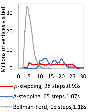
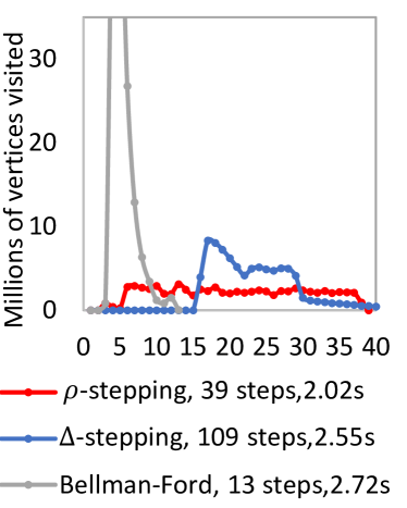
(a). TW	(b). FT	(c). WB	(d). USA

Figure 7. Number of visited vertices in each step in PQ-$\rho$, PQ-$\Delta^{*}$ and PQ-BF. Here we only run on one source vertex, since it has unclear meaning to compute the average of multiple runs on each step. Hence, the runtimes can be different from Table 4 (average on 100 runs from 10 source vertices), and some curves are bumpy. We use 96 cores (192 hyperthreads).

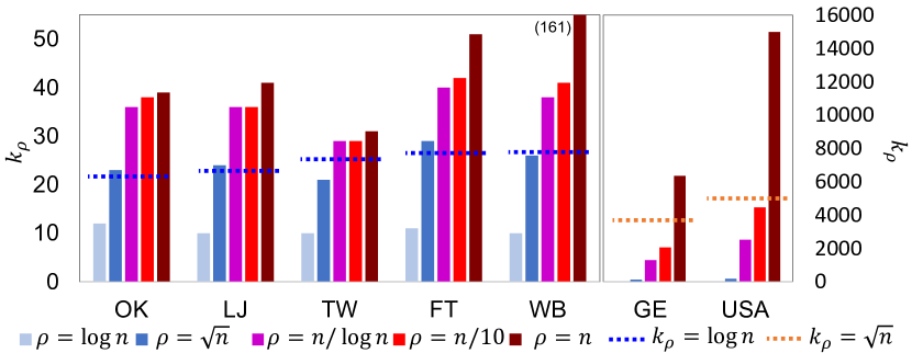
Figure 8. The values of $k_{\rho}$ with different values of $\rho$ for different graphs.

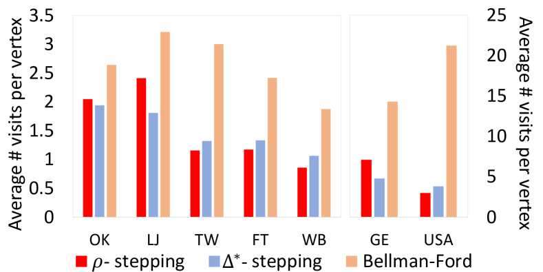
Figure 9. Number of visits per vertex and per edge, respectively, for PQ-$\rho$, PQ-$\Delta^{*}$ and PQ-BF on all graphs.

Number of visits to vertices. Unlike Dijkstra, other parallel SSSP algorithms can visit each vertex or edge more than once. While this allows for parallelism, the total work is also increased. To show how much “redundant” work is done for the stepping algorithms, we measure the average number of visits per vertex (Fig. 9), and the number of visited vertices in each step on four representative graphs (Fig. 9) . We show results for four representative graphs, and full results are in Fig. 9. We note that the other systems vary a lot in implementation details, and it is hard to directly measure these quantities from their code. Hence, we compare among our implementations. For the same reason, PQ-$\Delta^{*}$ may not precisely reflect the numbers of other $\Delta$-Stepping implementations. In this paragraph, we first focus on the scale-free networks, and discuss road graphs later.

Figure 9 shows the average number of visits per vertex. On the two small graphs (OK and LJ), since the work cannot saturate all 192 threads, both PQ-$\Delta^{*}$ and PQ-$\rho$ act similar to Bellman-Ford to maximize parallelism. For the three larger graphs (TW, FT, and WB), PQ-$\rho$ always triggers the smallest average visit to vertices and edges. The trend showed in Fig. 9 exactly matches the sequential time of each implementation. Hence, one advantage of PQ-$\rho$ over PQ-BF and PQ-$\Delta^{*}$ on scale-free networks is less total work.

Figure 9 shows the number of visited vertices per step. In PQ-BF, the numbers always grow quickly to a large value, stay for a few steps, and finish quickly. Although usually using the fewest steps, PQ-BF is the slowest, since the dense steps cause many redundant relaxations. PQ-$\Delta^{*}$ usually uses more steps than both PQ-BF and PQ-$\rho$. In most of the steps (at the beginning and the end), PQ-$\Delta^{*}$ visits only a small number of vertices, but the peak values are much higher than PQ-$\rho$. PQ-$\rho$ shows a more even pattern across the steps: in most of the steps, it processes a moderate number of vertices, and the peak value is much smaller than PQ-$\Delta^{*}$ or PQ-BF.

These patterns in Fig. 9 reflect the nature of the three algorithms. Bellman-Ford always visits all vertices in the frontier in each step. This created significant redundant work. $\Delta^{*}$-Stepping controls work-span tradeoff based on distances. On scale-free networks, it reaches the peak work in some middle steps, which is significantly higher than other steps. $\rho$-Stepping controls the work-span tradeoff using the number of vertices processed per step. We believe on scale-free networks, this quantity is a closer indicator to the actual “work” in each step than the distance gap is. In other words, $\rho$-Stepping controls the work in each step that is minimal to saturate all processors, so it explores sufficient parallelism with minimized redundant work.

$k$-$\rho$ property for different graphs. To better understand the properties of different graphs, we show the $\rho$-$k_{\rho}$ curves in Fig. 9. We note that computing the exact value of $k_{\rho}$ is expensive (which makes Radius-Stepping impractical), and we estimate the value using 100 samples. As mentioned, this indicates how much potential parallelism we can get on the original graph (i.e., without shortcuts). We show the value of $k_{\rho}$ when $\rho$ is $\log n$, $\sqrt{n}$, $n/\log n$, $n/10$, and $n$, respectively. Note that $k_{n}$ is the shortest path tree depth.

On all scale-free networks, we observe that $k_{n}$ is $O(\log n)$ (about $2\log n$). Interestingly, all scale-free networks are $(\log n,\sqrt{n})$-graph, which means that almost all vertices can reach their $\sqrt{n}$ nearest vertices by $\log n$ hops. This is not surprising for scale-free networks, which have some “hubs” that are well connected to other vertices. These vertices are easy to be reached by any source in a few steps. Once reached, they can reach a lot of other vertices, which quickly accumulate $\sqrt{n}$ nearest neighbors for any source. The road graphs have a different $\rho$-$k_{\rho}$ pattern. On GE and USA, it takes more than $100$ hops to reach $\sqrt{n}$ nearest vertices, and $O(\sqrt{n})$ steps to reach $O(n)$ nearest vertices. We believe the result is reasonable since road graphs are (almost) planar graphs.

Discussions for Road Graphs. Road graphs are (almost) planar and have different $k$-$\rho$ patterns than other graphs, and the shortest-path trees are deep and slim. Hence, without the special optimizations (e.g., in Ligra and Julienne), the performance is slow. As mentioned in Sec. 6, our optimization expands multiple levels in the shortest-path tree in one step. This makes the performance of our implementations competitive or better than GAPBS and Galois.

On road graphs, PQ-$\Delta^{*}$ is the fastest. This somehow indicates that expanding with distance may be a good strategy for road graphs. One possible reason is that they are planar graphs with Euclidean distance. Hence, setting fixed-width “annuli” seems a reasonable work-parallelism tradeoff, when using a proper $\Delta$. Since the frontier on road graphs is small, PQ-$\rho$ has insufficient frontier size in each step for enough parallelism. Hence, it is hard for PQ-$\rho$ to control the number of vertices visited precisely, and the performance is slightly slower than PQ-$\Delta^{*}$. However, PQ-$\rho$ has more stable performance than PQ-$\Delta^{*}$ in the parameter space (Figs. 1 and 2).

$\Delta$-Stepping and $\Delta$. We test all $\Delta$-Stepping algorithms with varying $\Delta$ on all graphs. For each test case, we normalize the running time to the best time across all $\Delta$ values. For page limit, we present four graphs in Fig. 1, and the full results in the full paper (ssspfull, ).

Friendster (FT):
GAPBS	Galois	Julinne	Ours (PQ-$\Delta^{*}$)
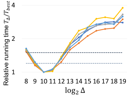
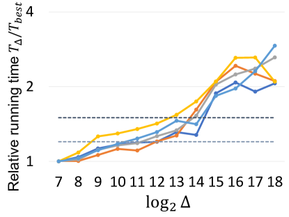
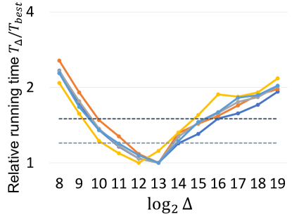
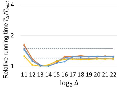
WebGraph (WB):
GAPBS	Galois	Julinne	Ours (PQ-$\Delta^{*}$)

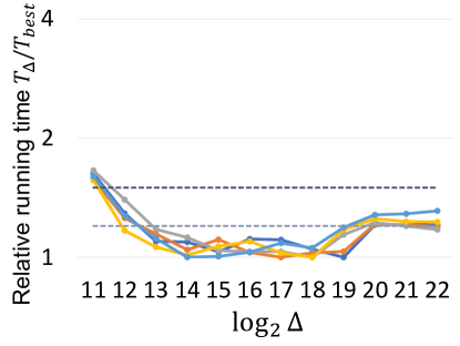
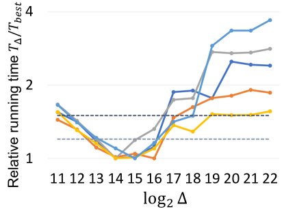
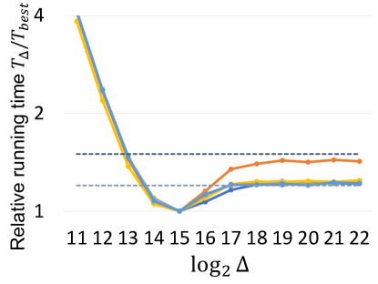
Figure 13. Relative running time with varying $\Delta$ of multiple $\Delta$-Stepping implementations on different sources. The five lines with different colors represent five sources. For each source, we normalize the running time to the corresponding fastest time. For each of the implementations, we use a window of $2^{11}$ around the best value of $\Delta$. The best value of $\Delta$ is relatively stable for all implementations, except for a few instances (e.g., GAPBS and Julienne on WebGraph). Generally speaking, the best $\Delta$ for one source node makes another node at most 20% slower. Also, it seems the result on directed graphs (WB) is more unstable than undirected graphs (FT). On both WB and FT, our PQ-$\Delta^{*}$ based on $\Delta^{*}$-Stepping shows very stable performance.

On the same graph, the best choice of $\Delta$ varies a lot for different systems. On TW, Julienne’s best $\Delta$ is $2^{12}\times$ larger than Galois’s. The best $\Delta$ for one system can make another system up to $4\times$ slower. The selection of $\Delta$ in one system does not generalize to other systems. Secondly, even though all scale-free networks have the same edge weight distribution, for the same implementation, the best choice of $\Delta$ varies a lot on different graphs. Therefore, the selection of $\Delta$ on one graph does not generalize to other graphs. On the same graph, the performance is sensitive to the value of $\Delta$. Usually, $2$–$4\times$ off may lead to a 20% slowdown, and $4$–$8\times$ off may lead to a 50% slowdown. A badly-chosen $\Delta$ can largely affect the performance. As a result, for every graph-implementation combination, we have to search the best parameter $\Delta$. Fortunately, we find out that different sources show relatively stable performance for the same implementation-graph pair. This is also the conventional way of tuning $\Delta$ (we also did so). We present the results in Fig. 13.

Also, for almost all systems, the performance on road graphs is more sensitive to the value of $\Delta$ than on scale-free networks.

$\rho$-Stepping and $\rho$. We test $\rho$-Stepping with varying $\rho$. When $\rho$ is small, the running time increases significantly. This is also due to the lack of parallelism (similar to when $\Delta$-Stepping uses small $\Delta$). When $\rho$ gets large, the performance drops by no more than 20%. The best choices of $\rho$ are very consistent on different graphs. This is because the choice of $\rho$ in practice depends on the right level of parallelism we want to achieve, instead of the graph structure or edge weight distribution. As discussed, $\rho$-Stepping distributes work more evenly to each step. The goal of setting $\rho$ is to enable enough work to exploit full parallelism in each step, but without introducing more redundant work. The performance on road graphs are less sensitive, probably because the frontier size seldom reaches $\rho$ in road graphs. We also tested $\rho$-Stepping on various machines. We observe that the best choice of $\rho$ is still relatively consistent among different settings. We will present more results in the full paper.

Generally speaking, using large $\Delta$ or $\rho$ gives better (and more stable) performance than small $\Delta$ or $\rho$ values. This is not surprising because when these parameters are large, $\Delta$-Stepping and $\rho$-Stepping degenerate to Bellman-Ford that still has reasonable performance on social networks. When the parameters are small, $\Delta$-Stepping and $\rho$-Stepping both degenerate to Dijkstra and loses parallelism.

Summary. In summary, our PQ-$\rho$ generally achieves the best performance on the five scale-free networks. On average of the five graphs, PQ-$\rho$ is 1.41-1.93$\times$ faster better than existing systems. On the two road graphs, PQ-$\Delta^{*}$ always has the best performance, which is at least 14% better than existing systems. The good performance of PQ-$\rho$ on scale-free networks comes from three aspects. The first is scalability, indicated by the good self-speedup. Secondly, it visits fewer vertices and edges on large scale-free networks, which indicates less overall work. Lastly, the work is more evenly distributed to each step, such that each step can exploit sufficient parallelism, and also avoid performing “ineffective” work to relax the neighbors of unsettled vertices. This also indicates that on scale-free networks with uniformly distributed edge weights, controlling the number of vertices visited per step is a good strategy. On road graphs with Euclidean distance, $\Delta$-Stepping shows better performance.

Our PQ-$\rho$ implementation generally shows stable performance across $\rho$ values on all tested graphs. A fixed $\rho$ almost always gives performance within 5% off the performance with the best $\rho$.

Finally, on all tested graphs, PQ-$\rho$ and PQ-$\Delta^{*}$ are faster than all existing SSSP implementations (except for RoadUSA, PQ-$\rho$ is 0.01s slower than Galois). PQ-BF is faster than Ligra on all graphs. This indicates the efficiency of the stepping algorithm framework on implementing and optimizing parallel SSSP algorithms.

8. Related Work on Parallel SSSP

Practical parallel SSSP implementations. There have been dozens of practical implementations of parallel SSSP. In this paper, we compared to a few of them. Galois (nguyen2013lightweight, ) uses an approximate priority queue ordered by integer metric with NUMA-optimization to improve the performance of SSSP. GraphIt (zhang2018graphit, ; zhang2020optimizing, ) proposed a priority queue abstraction and a new optimization, bucket fusion, to reduce the synchronization overhead of $\Delta^{*}$-Stepping. The optimizations are later adopted by GAPBS (beamer2015gap, ), which is the one we compared to. Julienne (dhulipala2017, ) proposed and used the bucketing data structure to order the vertices for $\Delta$-Stepping based on semisorting (gu2015top, ). Ligra (ShunB2013, ) includes one of the most efficient Bellman-Ford implementations.

There has also been a significant amount of work on other implementations, include those on the distributed setting (malewicz2010pregel, ; zhu2016gemini, ; besta2017push, ), GPUs (davidson2014work, ; wang2016gunrock, ), among many others. Our reported running time in this paper is much faster than in these papers on the same graphs, and comparing the superiorities of different settings on parallel SSSP is out of the scope of this paper. Parallel SSSP based on parallel priority queues are reviewed in Sec. 4.

Theoretical work on parallel SSSP. There has been a rich literature of theoretical parallel SSSP algorithms. Among them, many algorithms (ullman1991high, ; klein1997randomized, ; cohen1997using, ; Shi1999, ; cohen2000polylog, ; spencer1997time, ) achieve very similar bounds to Radius-Stepping (blelloch2016parallel, ) we discussed in this paper, but require adding shortcut edges. Basically the product of work and span is $\tilde{\Theta}(nm)$ (referred to as the transitive closure bottleneck (KarpR90, )). Some algorithms are analyzed based on edge weights (meyer2002buckets, ; meyer2001heaps, ), and many others are on approximate shortest-paths (elkin2019hopsets, ; miller2015improved, ; cao2020efficient, ; li2020faster, ; andoni2020parallel, ) and other models (augustine2020shortest, ; kuhn2020computing, ; ghaffari2018improved, ). While these algorithms are insightful, to the best of our knowledge, none of them have implementations.

Appendix A Lower Bound for Batch-Update Work

We now show that in order to preserve the total ordering of all records, we need at least $O(\log(n+b))$ work per update, where $n$ is the number of records in the priority queue. For a batch update of $b$ unordered records, there are ${b+n\choose b}\cdot b!$ total possible input cases. In the comparison model, the lower bound for work of the batch update is:

$$\log_{2}\mathopen{}\mathclose{{}\left({{b+n\choose b}\cdot b!}}\right)= \log_{2}\mathopen{}\mathclose{{}\left({(b+n)!\over b!n!}\cdot b!}\right)$$

$$= \log_{2}\mathopen{}\mathclose{{}\left({\prod_{i=1}^{b}{(n+i)}}}\right)$$

$$= \Omega(b\log(n+b))$$

Hence, to achieve better bounds, like in Thm. 4.1, we cannot maintain the total ordering of all records.

Appendix B Finding the $\rho$-th Element in a List

We now discuss how to find the $\rho$-th element in a list, which is used in $\rho$-Stepping. One solution is to pick $s=c(n/\rho+\log n)$ random samples where $c>1$ is a constant. We can then sort the samples and pick the $(\rho s/n)$-th one. By setting up the parameters correctly and using Chernoff Bound, we can show that with high probability, the selected output is within $(1-\epsilon)\rho$-th and $(1+\epsilon)\rho$-th element for some constant $0<\epsilon<1$. We can check if the output is in this range by calling Extract of the LaB-PQ, and if not, we can just retry until succeed. We note that instead of finding the exact $\rho$-th element, using an approximate $\rho^{\prime}$-th element within a constant factor of $\rho$ will not affect any bounds for $\rho$-Stepping. In practice, we set $c=10$ and run the entire sampling algorithm sequentially, and this simple approach always gives a satisfactory output. However, the work and span bounds are high probability bounds, instead of deterministic bounds. Also, it only applies to the case when $\rho=\Omega(\sqrt{n})$. Otherwise, the sorting cost will dominate.

We are aware of a data structure [2] (unpublished work) that can find the $\rho$-th element in a list efficiently. More accurately, it takes $O(\rho)$ work and $O(\log n)$ span to find an approximate $\rho$-th element, and $O(\log(n/b))$ work per element in a batch insertion or a batch deletion of $b$ elements. Basically, this is a blocked linked list data structure that looks like a binary search tree, but each leaf contains a block of $[\rho,3\rho]$ unsorted elements. When the leaf grows too big or too small, we split or merge it with an amortized constant work per update and $O(\log n)$ span. Hence, the cost per update is $O(\log(n/b))$ (to find the leaf node) plus a constant (amortized work for future leaf split or merge). Since the first leaf contains the smallest $\rho$ to $3\rho$ records, we can just pick the largest key among this leaf. This gives us a key ranked within $\rho$ and $3\rho$, with the exception if we have fewer than $\rho$ records in total (in this case the largest is returned).

Using this data structure requires some changes since we have to explicitly generate the batch of updates (relaxations). Theoretically, this is achievable as described below, but in practice the overhead can be significant so we do not use it. This step is essentially Ligra’s approach to generate the next frontier [80]. For each step, we allocate an array, and the size is the number of total neighbors of the vertices processed in this step. Then we mark a flag for each successful relaxation, and after all relaxations are completed, we pack this array, and this is the batch of updates that applies to the next frontier (the priority queue in our case). This step takes linear work and logarithmic span, so the cost is asymptotically bounded by the relaxation cost.

Appendix C Applying LaB-PQ to Shi-Spencer

Shi-Spencer algorithm [79] is a parallel SSSP algorithm with theoretical guarantee. This algorithm is complicated, which harms its practicability. We note that if we use our tournament-tree-based LaB-PQs to replace the parallel search trees in Shi-Spencer algorithm, we can improve the work bound by up to a logarithmic factor. This algorithm needs preprocessing to shortcut each vertex to its $\rho$ nearest vertices.

The main bottleneck in Shi-Spencer algorithm is to maintain a binary search tree for each vertex that keeps track of its $\rho$ nearest neighbors. Once a vertex is settled, it will be removed from all the lists of their neighbors. Such removals can happen for $O(m+n\rho)$ times in total. The algorithm requires querying and extracting the $\rho$ nearest vertices of a vertex, which is used for $O(n)$ times in total. In their original algorithm, they use parallel 2-3 trees to maintain the closest neighbor sets, which incur a logarithmic cost per update.

We note that the functionalities can be implemented by our tournament tree-based LaB-PQs. More importantly, similar to the stepping algorithms, since there are more updates than extractions, we can apply the updates lazily for better work efficiency. In this case, the worst case is all the updates distribute evenly—each extract needs to first lazily update $O(m/n+\rho)$ previous updates and then apply the $O(n)$ extractions. By the distribution lemma (Lem. 5.2), the total work is:

$$O\mathopen{}\mathclose{{}\left((m+n\rho)\log\frac{n\cdot n}{m+n\rho}}\right)=O\mathopen{}\mathclose{{}\left((m+n\rho)\log\frac{n^{2}}{m+n\rho}}\right)$$

Hence, for dense graphs or if the algorithm picks a large $\rho$, the new work can be improved by up to a logarithm factor. We note that a few other search trees and data structures are maintained in Shi-Spencer, but the total cost is asymptotically bounded by the cost discussed in the above paragraph.

Appendix D Fully Dynamic LaB-PQ

In Sec. 4 we discuss and analyze the LaB-PQ’s implementations assuming the universe of the records has a fixed size $n$, which is $|V|$ for SSSP. This is good enough to derive the bounds in Tab. 3. However, we note that it is not hard to extend our algorithms to deal with the case without this assumption.

To do so, we need an explicit batch of updates, which can include insertions, deletions, and/or just key updates. Our algorithm will in turn process the same type of operations. For insertions (say $k$ in total), we can grow the tree size from $2n-1$ to $2(n+k)-1$, copy the leaf nodes from the range of $n$ to $n+k-1$ to the range of $2n$ to $2n+k-1$, insert the new keys to the range of $2n+k$ to $2(n+k)-1$ ($k$ in total), and update the corresponding tree paths. The cost for $k$ insertions is $O(k+\log n)$. For deletions (again, say $k$ in total), we can use the last tree leaves to fill in the holes for the deletions, and update the tree paths. The cost for $k$ deletions is $O(k\log(n/k))$. For updates, we can directly apply Algorithm 2. All of them can be parallelized and have $O(\log n)$ span by a divide-and-conquer approach to update tree paths.

Appendix E Implementation Details for Resizable Hash Tables

As mentioned in Sec. 6, we use a resizable hash table next_frontier to maintain the frontier in our sparse version of stepping algorithm implementations. Whenever a vertex $v$ is to be added to the next frontier, we pick a slot $i$ uniformly at random, and attempt to write $v$ to next_frontier[i] using compare_and_swap, and use linear probing if there is collision or conflict due to concurrency. During the process, we keep an estimation of the size of next_frontier, and resize accordingly. For frontier size $s$, the space used by the hash table is always $O(s)$. We use two hash tables, alternating them to be the current and next frontiers.

It is worth noting that, even in resizing we do not explicitly allocate memory or move data. We will start with allocating an array of size $n$, and adjust tail pointer of the array to control the current hash table size. When the load factor of the current hash table reaches a pre-defined constant, we enlarge the hash table. We do this by moving the tail pointer to be twice the current size, and let all future scatters go to the last half of the hash table. For each step, we always start from a pre-defined MIN_SIZE of the hash table. Since we only insert to the hash table, we do not need to shrink the hash table. We show a pseudocode below to illustrate the process.

hash_table {
  vertex* table;
  int offset, tail, est_size;
  double SAMPLE_RATE;
  int MIN_SIZE;

  hash_table(int n) {
    table = new vertex[n];
    init(); }

  increment_size() {
    if (flip_coin(SAMPLE_RATE)) fetch_and_add(&est_size);}

  init() {offset = 0; tail = MIN_SIZE;}

  insert(vertex u) {
    slot = random_slot(u) + offset;
    while(!CAS(&table[slot], empty, u))
      slot = next_slot(slot);
    increment_size();
    if (size > est_size) {
      offset = tail;
      tail = tail*2; }
  }
};

hash_table* current_frontier, next_frontier;

parallel_for (v in current_frontier) {
  parallel_for (u is v’s out-neighbor) {
    if (v relaxes u) {
      next_frontier.insert(u);
    } } }
swap(current_frontier, next_frontier);
next_frontier->init();

Appendix F Experiment on Different Implementations for LaB-PQ

We also use a simple experiment to test the relative performance of array-based and tournament tree-based LaB-PQ. We note that for Update, our array-based implementation uses a hash-table-like data structure, which is only $O(1)$ work per insertion, while tournament tree needs up to logarithmic work. For Extract, the array-based implementation needs $O(n)$ time, while tournament tree needs $O(\rho\log(n/\rho))$ time to extract the top $\rho$ records. To estimate which one will give better performance in practice, we simulate the Extract function and compare the performance for the two data structures.

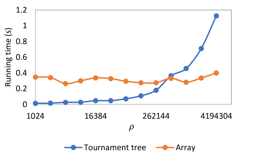
Figure 10. Running time of extracting $\rho$ elements from tournament tree- and array- based implementation of LaB-PQ, respectively.

To test the performance of Extract, we vary the value of $\rho$. We first initialize the priority queue with $n=10^{8}$ records, which is about the same order of magnitude as the number of vertices in the graphs we tested. Our tournament tree is also implemented in flat arrays, avoiding expensive pointer-based structure. We accumulate 10 runs of Extract. The result is shown in Fig. 10. The running time of array-based implementation is stable and is always around 0.35s. This is because the cost of array-based LaB-PQ is $O(n)$, which is not affected by the value of $\rho$. The cost of the tournament tree increases with the value of $\rho$. When $\rho$ is larger than $2^{19}$, the array-based implementation achieves better performance. We note that the setting is advantageous to tournament tree-based implementation since we do not consider the update cost ($O(1)$ for arrays and $O(\log n)$ for tournament trees), and we always assume the frontier size to be large ($10^{8}$). For the social networks we tested, the value of $\rho$ is usually larger than $2^{19}$. Therefore we always use array-based implementation of LaB-PQ. For the road graphs, the value of $\rho$ is slightly below $2^{19}$. As mentioned, this experiment does not consider update cost. Also, on road networks, the frontier size is also smaller (much smaller than $10^{8}$), which is favorable to array-based implementation. Based on these reasons, we choose to use the array-based data structures to implement our stepping algorithms. From Fig. 9, for $\Delta$-Stepping, in the dense rounds (which dominate total running time), the number of vertices to be extracted is also reasonably large. It is an interesting future work to see if tournament tree-based implementation can be more efficient on certain graphs that prefer a small $\rho$ in $\rho$-Stepping.

Appendix G Experiment on different source vertices

In previous experiments, we show the average running time on multiple source vertices on each graph. Now we show if different algorithms perform differently from the sources on the same graph. To do so, we randomly pick 100 source vertices in Friendster and Twitter, and test the performance from each of them. The results in shown in Fig. 11. Although the running time on these vertices and graphs differs, we can see that $\rho$-Stepping is consistently faster than the other two implementations, except for four vertices in Twitter. We conclude that starting from fringe vertices and hub vertices does not make a significant difference in the relative performance between Bellman-Ford, $\Delta^{*}$-stepping, and $\rho$-Stepping.

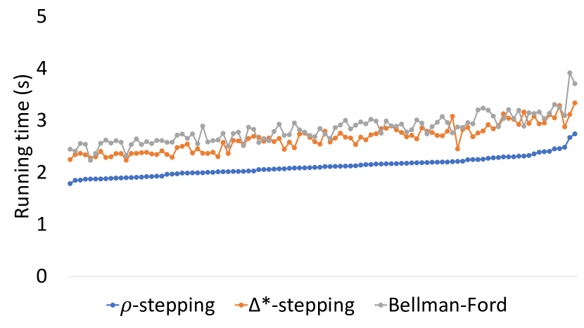
(a). FT

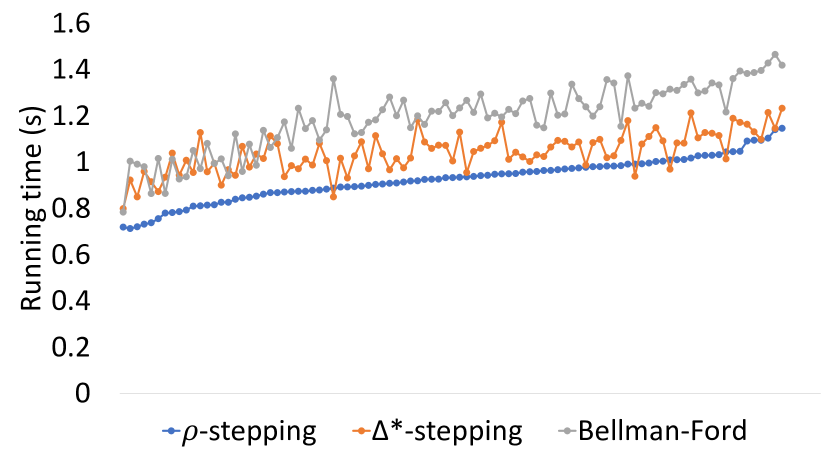
(b). TW

Figure 11. Running time on difference source vertices.

Appendix H Experiment on a different machine

We also experiment on whether different machines affect the best $\rho$ choice. We launched a virtual machine in Amazon Web Services (AWS). This single-socket machine is equipped with Intel Xeon Platinum 8175M CPUs with a total of 24 cores (48 hyperthreads). It has 192GB of main memory and 33MB L3 cache. Other setting is the same as the previous experiments as mentioned in Tab. 4. We present the result in Fig. 12. Surprisingly, we found out that taking $\rho=2^{21}$ (or any value between $2^{20}$ to $2^{22}$) is still a good choice for all graphs for this different machine, although it has much fewer cores. Comparing Figs. 12 and 2, the machine with fewer cores shows a less stable performance especially when $\rho$ is small. We note that there are also other parameters in the implementation that may affect the pattern of the relative performance of different $\rho$ values (e.g., the sparse-dense threshold). In general, we do note that different hardware settings (e.g., cache size, number of sockets, number of threads) can affect the relative performance with different values of $\rho$, which is more significant for the smaller values of $\rho$.

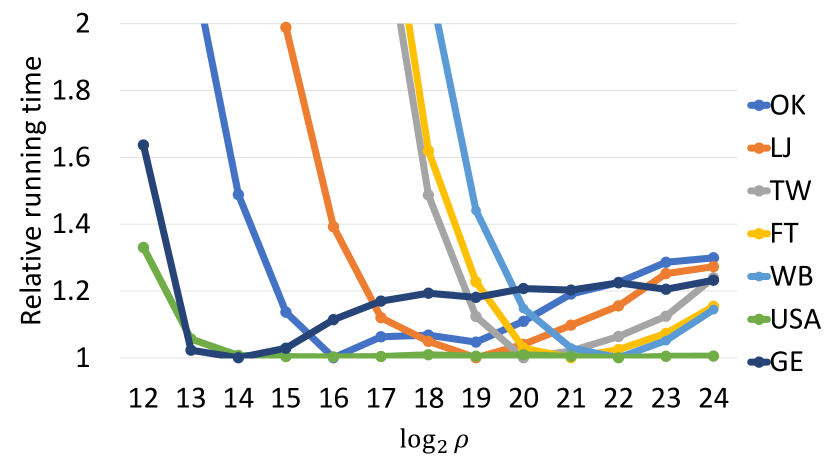
Figure 12. Relative running time of $\rho$-Stepping with varied $\rho$ on the AWS machine.

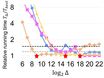
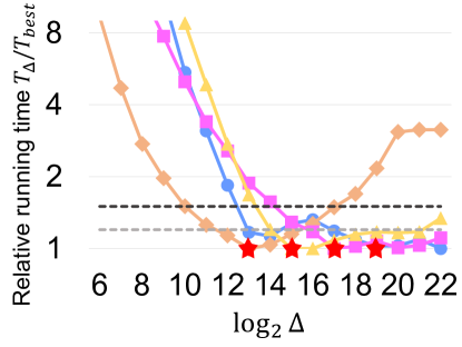
(a). OK	(b). LJ	(c). TW	(d). FT

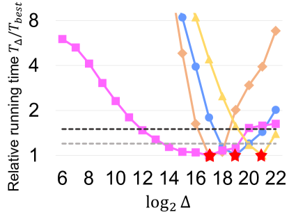
(e). WB	(f). GE	(g). USA

Figure 14. $\Delta$-stepping relative running time with varying $\Delta$. We use 96 cores (192 hyperthreads).

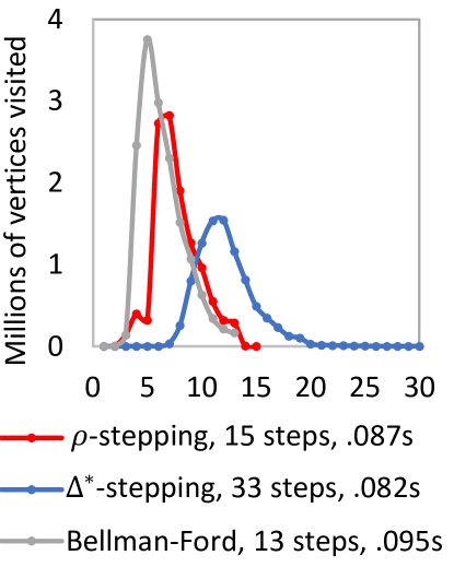
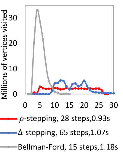
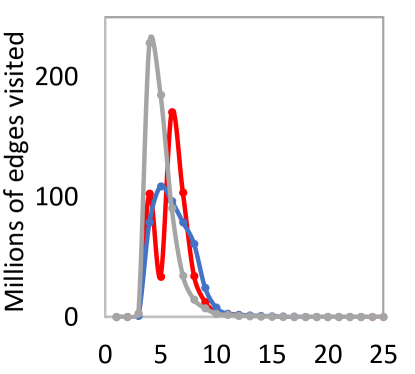
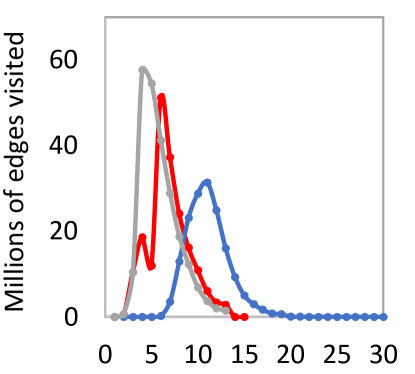
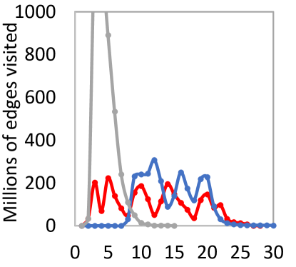
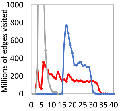
(a). OK	(b). LJ	(c). TW	(d). FT

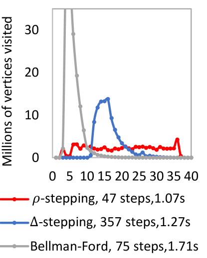
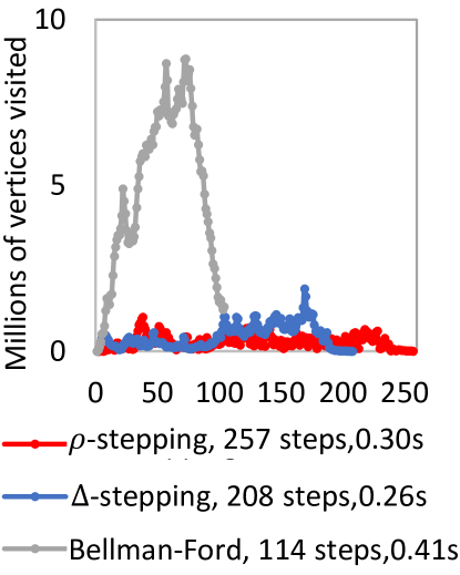
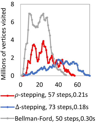
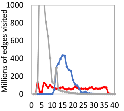
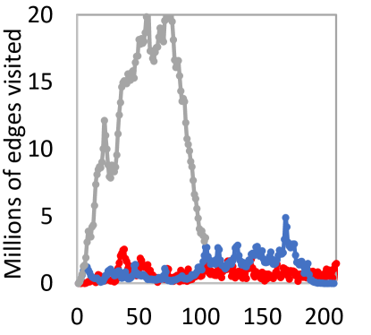
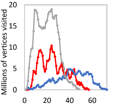
(e). WB	(f). USA	(g). GE

Figure 15. Number of visited vertices in each step in PQ-$\rho$, PQ-$\Delta^{*}$ and PQ-BF. Here we only run on one source vertex, since it has unclear meaning to compute the average of multiple runs on each step. Hence, the runtimes can be different from Table 4 (average on 100 runs from 10 source vertices), and some curves are bumpy. We use 96 cores (192 hyperthreads).

References

- [1] Openstreetmap © openstreetmap contributors. https://www.openstreetmap.org/, 2010.
- [2] Efficient parallel ordered maps using compressed search trees. 2021.
- [3] U. A. Acar, D. Anderson, G. E. Blelloch, and L. Dhulipala. Parallel batch-dynamic graph connectivity. In ACM Symposium on Parallelism in Algorithms and Architectures, pages 381–392, 2019.
- [4] U. A. Acar, G. E. Blelloch, and R. D. Blumofe. The data locality of work stealing. Theoretical Computer Science (TCS), 35(3), 2002.
- [5] K. Agrawal, J. T. Fineman, K. Lu, B. Sheridan, J. Sukha, and R. Utterback. Provably good scheduling for parallel programs that use data structures through implicit batching. In ACM Symposium on Parallelism in Algorithms and Architectures (SPAA), 2014.
- [6] D. Alistarh, J. Kopinsky, J. Li, and N. Shavit. The spraylist: A scalable relaxed priority queue. In ACM Symposium on Principles and Practice of Parallel Programming (PPOPP), pages 11–20, 2015.
- [7] D. Anderson, G. E. Blelloch, and K. Tangwongsan. Work-efficient batch-incremental minimum spanning trees with applications to the sliding-window model. In ACM Symposium on Parallelism in Algorithms and Architectures (SPAA), 2020.
- [8] A. Andoni, C. Stein, and P. Zhong. Parallel approximate undirected shortest paths via low hop emulators. In ACM Symposium on Theory of Computing (STOC), pages 322–335, 2020.
- [9] J. Augustine, K. Hinnenthal, F. Kuhn, C. Scheideler, and P. Schneider. Shortest paths in a hybrid network model. In ACM-SIAM Symposium on Discrete Algorithms (SODA), pages 1280–1299. SIAM, 2020.
- [10] L. Backstrom, D. Huttenlocher, J. Kleinberg, and X. Lan. Group formation in large social networks: membership, growth, and evolution. In ACM International Conference on Knowledge Discovery and Data Mining (SIGKDD), pages 44–54, 2006.
- [11] A. Bäumker, W. Dittrich, F. Meyer, and I. Rieping. Realistic parallel algorithms: Priority queue operations and selection for the bsp* model. In European Conference on Parallel Processing, pages 369–376. Springer, 1996.
- [12] S. Beamer, K. Asanović, and D. Patterson. The gap benchmark suite. arXiv preprint arXiv:1508.03619, 2015.
- [13] R. Bellman. On a routing problem. Quarterly of applied mathematics, 16(1):87–90, 1958.
- [14] N. Ben-David, G. E. Blelloch, J. T. Fineman, P. B. Gibbons, Y. Gu, C. McGuffey, and J. Shun. Parallel algorithms for asymmetric read-write costs. In ACM Symposium on Parallelism in Algorithms and Architectures (SPAA), 2016.
- [15] N. Ben-David, G. E. Blelloch, J. T. Fineman, P. B. Gibbons, Y. Gu, C. McGuffey, and J. Shun. Implicit decomposition for write-efficient connectivity algorithms. In IEEE International Parallel and Distributed Processing Symposium (IPDPS), 2018.
- [16] M. Besta, M. Podstawski, L. Groner, E. Solomonik, and T. Hoefler. To push or to pull: On reducing communication and synchronization in graph computations. In International Symposium on High-Performance Parallel and Distributed Computing (HPDC), pages 93–104, 2017.
- [17] T. Bingmann, T. Keh, and P. Sanders. A bulk-parallel priority queue in external memory with stxxl. In International Symposium on Experimental Algorithms (SEA), pages 28–40. Springer, 2015.
- [18] G. E. Blelloch, R. A. Chowdhury, P. B. Gibbons, V. Ramachandran, S. Chen, and M. Kozuch. Provably good multicore cache performance for divide-and-conquer algorithms. In ACM-SIAM Symposium on Discrete Algorithms (SODA), 2008.
- [19] G. E. Blelloch, D. Ferizovic, and Y. Sun. Just join for parallel ordered sets. In ACM Symposium on Parallelism in Algorithms and Architectures (SPAA), 2016.
- [20] G. E. Blelloch, J. T. Fineman, P. B. Gibbons, and H. V. Simhadri. Scheduling irregular parallel computations on hierarchical caches. In ACM Symposium on Parallelism in Algorithms and Architectures (SPAA), 2011.
- [21] G. E. Blelloch, J. T. Fineman, Y. Gu, and Y. Sun. Optimal parallel algorithms in the binary-forking model. In ACM Symposium on Parallelism in Algorithms and Architectures (SPAA), 2020.
- [22] G. E. Blelloch and P. B. Gibbons. Effectively sharing a cache among threads. In ACM Symposium on Parallelism in Algorithms and Architectures (SPAA), 2004.
- [23] G. E. Blelloch, P. B. Gibbons, and H. V. Simhadri. Low depth cache-oblivious algorithms. In ACM Symposium on Parallelism in Algorithms and Architectures (SPAA), 2010.
- [24] G. E. Blelloch, Y. Gu, J. Shun, and Y. Sun. Parallel write-efficient algorithms and data structures for computational geometry. In ACM Symposium on Parallelism in Algorithms and Architectures (SPAA), 2018.
- [25] G. E. Blelloch, Y. Gu, J. Shun, and Y. Sun. Randomized incremental convex hull is highly parallel. In ACM Symposium on Parallelism in Algorithms and Architectures (SPAA), 2020.
- [26] G. E. Blelloch, Y. Gu, Y. Sun, and K. Tangwongsan. Parallel shortest paths using radius stepping. In ACM Symposium on Parallelism in Algorithms and Architectures (SPAA), 2016.
- [27] G. E. Blelloch and M. Reid-Miller. Fast set operations using treaps. In ACM Symposium on Parallelism in Algorithms and Architectures (SPAA), 1998.
- [28] G. E. Blelloch and M. Reid-Miller. Pipelining with futures. Theory of Computing Systems (TOCS), 32(3), 1999.
- [29] G. E. Blelloch, H. V. Simhadri, and K. Tangwongsan. Parallel and I/O efficient set covering algorithms. In ACM Symposium on Parallelism in Algorithms and Architectures (SPAA), 2012.
- [30] G. S. Brodal, J. L. Träff, and C. D. Zaroliagis. A parallel priority queue with constant time operations. Journal of Parallel and Distributed Computing, 49(1):4–21, 1998.
- [31] I. Calciu, H. Mendes, and M. Herlihy. The adaptive priority queue with elimination and combining. In International Symposium on Distributed Computing (DISC), pages 406–420. Springer, 2014.
- [32] N. Cao, J. T. Fineman, and K. Russell. Efficient construction of directed hopsets and parallel approximate shortest paths. In ACM Symposium on Theory of Computing (STOC), pages 336–349, 2020.
- [33] D. Z. Chen and X. S. Hu. Fast and efficient operations on parallel priority queues. In International Symposium on Algorithms and Computation, pages 279–287. Springer, 1994.
- [34] R. Chowdhury, P. Ganapathi, Y. Tang, and J. J. Tithi. Provably efficient scheduling of cache-oblivious wavefront algorithms. In ACM Symposium on Parallelism in Algorithms and Architectures (SPAA), pages 339–350, 2017.
- [35] R. A. Chowdhury, V. Ramachandran, F. Silvestri, and B. Blakeley. Oblivious algorithms for multicores and networks of processors. Journal of Parallel and Distributed Computing, 73(7):911–925, 2013.
- [36] E. Cohen. Using selective path-doubling for parallel shortest-path computations. Journal of Algorithms, 22(1):30–56, 1997.
- [37] E. Cohen. Polylog-time and near-linear work approximation scheme for undirected shortest paths. Journal of the ACM (JACM), 47(1):132–166, 2000.
- [38] R. Cole and V. Ramachandran. Resource oblivious sorting on multicores. ACM Transactions on Parallel Computing (TOPC), 3(4), 2017.
- [39] T. H. Cormen, C. E. Leiserson, R. L. Rivest, and C. Stein. Introduction to Algorithms (3rd edition). MIT Press, 2009.
- [40] A. Crauser, K. Mehlhorn, U. Meyer, and P. Sanders. A parallelization of dijkstra’s shortest path algorithm. In International Symposium on Mathematical Foundations of Computer Science, pages 722–731. Springer, 1998.
- [41] V. A. Crupi, S. K. Das, and M. C. Pinotti. Parallel and distributed meldable priority queues based on binomial heaps. In ICPP Workshop on Challenges for Parallel Processing, volume 1, pages 255–262. IEEE, 1996.
- [42] S. K. Das, M. C. Pinotti, and F. Sarkar. Optimal and load balanced mapping of parallel priority queues in hypercubes. IEEE Transactions on Parallel and Distributed Systems, 7(6):555–564, 1996.
- [43] A. Davidson, S. Baxter, M. Garland, and J. D. Owens. Work-efficient parallel gpu methods for single-source shortest paths. In IEEE International Parallel and Distributed Processing Symposium (IPDPS), pages 349–359. IEEE, 2014.
- [44] N. Deo and S. Prasad. Parallel heap: An optimal parallel priority queue. The Journal of Supercomputing, 6(1):87–98, 1992.
- [45] L. Dhulipala, G. E. Blelloch, and J. Shun. Julienne: A framework for parallel graph algorithms using work-efficient bucketing. In ACM Symposium on Parallelism in Algorithms and Architectures (SPAA), 2017.
- [46] L. Dhulipala, G. E. Blelloch, and J. Shun. Theoretically efficient parallel graph algorithms can be fast and scalable. In ACM Symposium on Parallelism in Algorithms and Architectures (SPAA), 2018.
- [47] L. Dhulipala, C. McGuffey, H. Kang, Y. Gu, G. E. Blelloch, P. B. Gibbons, and J. Shun. Semi-asymmetric parallel graph algorithms for nvrams. Proceedings of the VLDB Endowment (PVLDB), 13(9), 2020.
- [48] E. W. Dijkstra. A note on two problems in connexion with graphs. Numerische mathematik, 1(1), 1959.
- [49] D. Dinh, H. V. Simhadri, and Y. Tang. Extending the nested parallel model to the nested dataflow model with provably efficient schedulers. In ACM Symposium on Parallelism in Algorithms and Architectures (SPAA), 2016.
- [50] X. Dong, Y. Gu, Y. Sun, and Y. Zhang. Efficient stepping algorithms and implementations for parallel shortest paths. arXiv preprint 2105.06145, 2021.
- [51] M. Elkin and O. Neiman. Hopsets with constant hopbound, and applications to approximate shortest paths. SIAM Journal on Computing, 48(4):1436–1480, 2019.
- [52] L. R. Ford Jr. Network flow theory. Technical report, Rand Corp Santa Monica Ca, 1956.
- [53] M. L. Fredman and R. E. Tarjan. Fibonacci heaps and their uses in improved network optimization algorithms. J. ACM, 34(3), 1987.
- [54] M. Ghaffari and J. Li. Improved distributed algorithms for exact shortest paths. In ACM Symposium on Theory of Computing (STOC), pages 431–444, 2018.
- [55] Y. Gu, O. Obeya, and J. Shun. Parallel in-place algorithms: Theory and practice. pages 114–128, 2021.
- [56] Y. Gu, J. Shun, Y. Sun, and G. E. Blelloch. A top-down parallel semisort. In ACM Symposium on Parallelism in Algorithms and Architectures (SPAA), 2015.
- [57] T. A. Henzinger, C. M. Kirsch, H. Payer, A. Sezgin, and A. Sokolova. Quantitative relaxation of concurrent data structures. In ACM Symposium on Principles of Programming Languages (POPL), pages 317–328, 2013.
- [58] R. M. Karp and V. Ramachandran. Parallel algorithms for shared-memory machines. In Handbook of Theoretical Computer Science, Volume A: Algorithms and Complexity (A). MIT Press, 1990.
- [59] P. N. Klein and S. Subramanian. A randomized parallel algorithm for single-source shortest paths. Journal of Algorithms, 25(2):205–220, 1997.
- [60] F. Kuhn and P. Schneider. Computing shortest paths and diameter in the hybrid network model. In ACM-SIAM Symposium on Discrete Algorithms (SODA), pages 109–118, 2020.
- [61] H. Kwak, C. Lee, H. Park, and S. Moon. What is twitter, a social network or a news media? In Proceedings of the 19th international conference on World wide web, pages 591–600, 2010.
- [62] J. Li. Faster parallel algorithm for approximate shortest path. In ACM Symposium on Theory of Computing (STOC), pages 308–321, 2020.
- [63] J. Lindén and B. Jonsson. A skiplist-based concurrent priority queue with minimal memory contention. In International Conference On Principles Of Distributed Systems, pages 206–220. Springer, 2013.
- [64] Y. Liu and M. Spear. A lock-free, array-based priority queue. In ACM Symposium on Principles and Practice of Parallel Programming (PPOPP), pages 323–324, 2012.
- [65] G. Malewicz, M. H. Austern, A. J. Bik, J. C. Dehnert, I. Horn, N. Leiser, and G. Czajkowski. Pregel: a system for large-scale graph processing. In Proceedings of the 2010 ACM SIGMOD International Conference on Management of data, pages 135–146, 2010.
- [66] R. Meusel, O. Lehmberg, and S. Bizer, Christian andVigna. Web data commons - hyperlink graphs. http://webdatacommons.org/hyperlinkgraph.
- [67] U. Meyer. Heaps are better than buckets: parallel shortest paths on unbalanced graphs. In European Conference on Parallel Processing, pages 343–351. Springer, 2001.
- [68] U. Meyer. Single-source shortest-paths on arbitrary directed graphs in linear average-case time. In ACM-SIAM Symposium on Discrete Algorithms (SODA), pages 797–806, 2001.
- [69] U. Meyer. Buckets strike back: Improved parallel shortest-paths. In IEEE International Parallel and Distributed Processing Symposium (IPDPS), pages 8–pp. IEEE, 2002.
- [70] U. Meyer and P. Sanders. -stepping: a parallelizable shortest path algorithm. Journal of Algorithms, 49(1):114–152, 2003.
- [71] G. L. Miller, R. Peng, A. Vladu, and S. C. Xu. Improved parallel algorithms for spanners and hopsets. In ACM Symposium on Parallelism in Algorithms and Architectures (SPAA), pages 192–201, 2015.
- [72] D. Nguyen, A. Lenharth, and K. Pingali. A lightweight infrastructure for graph analytics. In Proceedings of the Twenty-Fourth ACM Symposium on Operating Systems Principles, pages 456–471, 2013.
- [73] M. C. Pinotti and G. Pucci. Parallel priority queues. Information Processing Letters, 40(1):33–40, 1991.
- [74] A. Ranade, A. Cheng, E. Deprit, J. Jones, and S. Shih. Parallelism and locality in priority queues. In IEEE International Parallel and Distributed Processing Symposium (IPDPS), pages 490–496. IEEE, 1994.
- [75] P. Sanders. Fast priority queues for cached memory. J. Experimental Algorithmics.
- [76] P. Sanders. Randomized priority queues for fast parallel access. Journal of Parallel and Distributed Computing, 49(1):86–97, 1998.
- [77] P. Sanders, K. Mehlhorn, M. Dietzfelbinger, and R. Dementiev. Sequential and Parallel Algorithms and Data Structures. Springer.
- [78] N. Shavit and I. Lotan. Skiplist-based concurrent priority queues. In IEEE International Parallel and Distributed Processing Symposium (IPDPS), pages 263–268. IEEE, 2000.
- [79] H. Shi and T. H. Spencer. Time-work tradeoffs of the single-source shortest paths problem. Journal of Algorithms, 30(1):19–32, 1999.
- [80] J. Shun and G. E. Blelloch. Ligra: A lightweight graph processing framework for shared memory. In ACM Symposium on Principles and Practice of Parallel Programming (PPOPP), 2013.
- [81] J. Shun and G. E. Blelloch. Phase-concurrent hash tables for determinism. In ACM Symposium on Parallelism in Algorithms and Architectures (SPAA), pages 96–107, 2014.
- [82] T. H. Spencer. Time-work tradeoffs for parallel algorithms. jacm, 44(5):742–778, 1997.
- [83] Y. Sun and G. Blelloch. Implementing parallel and concurrent tree structures. In ACM Symposium on Principles and Practice of Parallel Programming (PPOPP), page 447–450, 2019.
- [84] Y. Sun and G. E. Blelloch. Parallel range, segment and rectangle queries with augmented maps. In SIAM Symposium on Algorithm Engineering and Experiments (ALENEX), pages 159–173, 2019.
- [85] Y. Sun, D. Ferizovic, and G. E. Blelloch. Pam: Parallel augmented maps. In ACM Symposium on Principles and Practice of Parallel Programming (PPOPP), 2018.
- [86] H. Sundell and P. Tsigas. Fast and lock-free concurrent priority queues for multi-thread systems. Journal of Parallel and Distributed Computing, 65(5):609–627, 2005.
- [87] T. Tseng, L. Dhulipala, and G. Blelloch. Batch-parallel euler tour trees. In 2019 Proceedings of the Twenty-First Workshop on Algorithm Engineering and Experiments (ALENEX), pages 92–106. SIAM, 2019.
- [88] J. D. Ullman and M. Yannakakis. High-probability parallel transitive-closure algorithms. SIAM Journal on Computing, 20(1):100–125, 1991.
- [89] Y. Wang, A. Davidson, Y. Pan, Y. Wu, A. Riffel, and J. D. Owens. Gunrock: A high-performance graph processing library on the gpu. In ACM Symposium on Principles and Practice of Parallel Programming (PPOPP), pages 1–12, 2016.
- [90] Y. Wang, S. Yu, Y. Gu, and J. Shun. A parallel batch-dynamic data structure for the closest pair problem. In ACM Symposium on Computational Geometry (SoCG), 2021.
- [91] J. Yang and J. Leskovec. Defining and evaluating network communities based on ground-truth. Knowledge and Information Systems, 42(1):181–213, 2015.
- [92] Y. Zhang, A. Brahmakshatriya, X. Chen, L. Dhulipala, S. Kamil, S. Amarasinghe, and J. Shun. Optimizing ordered graph algorithms with graphit. In ACM/IEEE International Symposium on Code Generation and Optimization (CGO), pages 158–170, 2020.
- [93] Y. Zhang, M. Yang, R. Baghdadi, S. Kamil, J. Shun, and S. Amarasinghe. Graphit: A high-performance graph dsl. Proceedings of the ACM on Programming Languages, 2(OOPSLA):1–30, 2018.
- [94] T. Zhou, M. Michael, and M. Spear. A practical, scalable, relaxed priority queue. In International Conference on Parallel Processing (ICPP), pages 1–10, 2019.
- [95] X. Zhu, W. Chen, W. Zheng, and X. Ma. Gemini: A computation-centric distributed graph processing system. In USENIX conference on Operating Systems Design and Implementation (OSDI), pages 301–316, 2016.