Value-at-Risk Optimization with Gaussian Processes
Abstract
Value-at-risk (VaR) is an established measure to assess risks in critical real-world applications with random environmental factors. This paper presents a novel VaR upper confidence bound (V-UCB) algorithm for maximizing the VaR of a black-box objective function with the first no-regret guarantee. To realize this, we first derive a confidence bound of VaR and then prove the existence of values of the environmental random variable (to be selected to achieve no regret) such that the confidence bound of VaR lies within that of the objective function evaluated at such values. Our V-UCB algorithm empirically demonstrates state-of-the-art performance in optimizing synthetic benchmark functions, a portfolio optimization problem, and a simulated robot task.
1 Introduction
Consider the problem of maximizing an expensive-to-compute black-box objective function that depends on an optimization variable and an environmental random variable . Due to the randomness in , the function evaluation of at is a random variable. Though for such an objective function , Bayesian optimization (BO) can be naturally applied to maximize its expectation over (Toscano-Palmerin & Frazier, 2018), this maximization objective overlooks the risks of potentially undesirable function evaluations. These risks can arise from either (a) the realization of an unknown distribution of or (b) the realization of the random given that the distribution of can be estimated well or that of is known. The issue (a) has been tackled by distributionally robust BO (Kirschner et al., 2020; Nguyen et al., 2020) which maximizes under the worst-case realization of the distribution of . To resolve the issue (b), the risk from the uncertainty in can be controlled via the mean-variance optimization framework (Iwazaki et al., 2020), value-at-risk (VaR), or conditional value-at-risk (CVaR) (Cakmak et al., 2020; Torossian et al., 2020). The work of Bogunovic et al. (2018) has considered adversarially robust BO, where is controlled by an adversary deterministically.111We use upper-case letter to denote the environmental random variable and lower-case letter to denote its realization or a (non-random) variable. In this case, the objective is to find that maximizes the function under the worst-case realization of , i.e., .
In this paper, we focus on case (b) where the distribution of is known (or well-estimated). For example, in agriculture, although farmers cannot control the temperature of an outdoor farm, its distribution can be estimated from historical data and controlled in an indoor environment for optimizing the plant yield. Given the distribution of , the objective is to control the risk that the function evaluation , for a sampled from , is small. One popular framework is to control the trade-off between the mean (viewed as reward) and the variance (viewed as risk) of the function evaluation with respect to (Iwazaki et al., 2020). However, quantifying the risk using variance implies indifference between positive and negative deviations from the mean, while people often have asymmetric risk attitudes (Goh et al., 2012). In our problem of maximizing the objective function, it is reasonable to assume that people are risk-averse towards only the negative deviations from the mean, i.e., the risk of getting lower function evaluations. Thus, it is more appropriate to adopt risk measures with this asymmetric property, such as value-at-risk (VaR) which is a widely adopted risk measure in real-world applications (e.g., banking (Basel Committee on Banking Supervision, 2006)). Intuitively, the risk that the random is less than VaR at level does not exceed , e.g., by specifying a small value of as , this risk is controlled to be at most . Therefore, to maximize the function while controlling the risk of undesirable (i.e., small) function evaluations, we aim to maximize VaR of the random function over .
The recent work of Cakmak et al. (2020) has used BO to maximize VaR and has achieved state-of-the-art empirical performances. They have assumed that we are able to select both and to query during BO, which is motivated by fact that physical experiments can usually be studied by simulation (Williams et al., 2000). In the example on agriculture given above, we can control the temperature, light and water () in a small indoor environment to optimize the amount of fertilizer (), which can then be used in an outdoor environment with random weather factors. Cakmak et al. (2020) have exploited the ability to select to model the function as a GP, which allows them to retain the appealing closed-form posterior belief of the objective function. To select the queries and , they have designed a one-step lookahead approach based on the well-known knowledge gradient (KG) acquisition function (Scott et al., 2011). However, the one-step lookahead incurs an expensive nested optimization procedure, which is computationally expensive and hence requires approximations. Besides, the acquisition function can only be approximated using samples of the objective function from the GP posterior and the environmental random variable . While they have analysed the asymptotically unbiased and consistent estimator of the gradients, it is challenging to obtain a guarantee for the convergence of their algorithm. Another recent work (Torossian et al., 2020) has also applied BO to maximize VaR using an asymmetric Laplace likelihood function and variational approximation of the posterior belief. However, in contrast to Cakmak et al. (2020) and our work, they have focused on a different setting where the realizations of are not observed.
In this paper, we adopt the setting of Cakmak et al. (2020) which allows us to choose both and to query, and assume that the distribution of is known or well-estimated. Our contributions include:
Firstly, we propose a novel BO algorithm named Value-at-risk Upper Confidence Bound (V-UCB) in Section 3. Unlike the work of Cakmak et al. (2020), V-UCB is equipped with a no-regret convergence guarantee and is more computationally efficient. To guide its query selection and facilitate its proof of the no-regret guarantee, the classical GP-UCB algorithm (Srinivas et al., 2010) constructs a confidence bound of the objective function. Similarly, to maximize the VaR of a random function, we, for the first time to the best of our knowledge, construct a confidence bound of VaR (Lemma 2). The resulting confidence bound of VaR naturally gives rise to a strategy to select . However, it remains a major challenge to select to preserve the no-regret convergence of GP-UCB. To this end, we firstly prove that our algorithm is no-regret as long as we ensure that at the selected , the confidence bound of VaR lies within the confidence bound of the objective function. Next, we also prove that this query selection strategy is feasible, i.e., such values of , referred to as lacing values (LV), exist.
Secondly, although our theoretical no-regret property allows the selection of any LV, we design a heuristic to select an LV such that it improves our empirical performance over random selection of LV (Section 3.3). We also discuss the implications when cannot be selected by BO and is instead randomly sampled by the environment during BO (Remark 1). Thirdly, we show that adversarially robust BO (Bogunovic et al., 2018) can be cast as a special case of our V-UCB when the risk level of VaR approaches from the right and the domain of is the support of . In this case, adversarially robust BO (Bogunovic et al., 2018) selects the same input queries as those selected by V-UCB since the set of LV collapse into the set of minimizers of the lower bound of the objective function (Section 3.4). Lastly, we provide practical techniques for implementing V-UCB with continuous random variable (Section 3.5): we (a) introduce local neural surrogate optimization with the pinball loss to optimize VaR, and (b) construct an objective function to search for an LV in the continuous support of .
The performance of our proposed algorithm is empirically demonstrated in optimizing several synthetic benchmark functions, a portfolio optimization problem, and a simulated robot task in Section 4.
2 Problem Statement and Background
Let the objective function be defined as where and are the bounded domain of the optimization variable and the support of the environmental random variable , respectively; and are the dimensions of and , respectively. The support of is defined as the smallest closed subset of such that . Let denote a realization of the random variable . Let denote a random variable whose randomness comes from . The VaR of at risk level is defined as:
| (1) |
which implies the risk that is less than its VaR at level does not exceed .
Our objective is to search for that maximizes at a user-specified risk level . Intuitively, the goal is find where the evaluations of the objective function are as large as possible under most realizations of the environmental random variable which is characterized by the probability of .
The unknown objective function is modeled with a GP. That is, every finite subset of follows a multivariate Gaussian distribution (Rasmussen & Williams, 2006). The GP is fully specified by its prior mean and covariance function for all in and in . For notational simplicity (and w.l.o.g.), the former is assumed to be zero, while we use the squared exponential (SE) kernel as its bounded maximum information gain can be used for later analysis (Srinivas et al., 2010).
To identify the optimal , BO algorithm selects an input query in the -th iteration to obtain a noisy function evaluation where are i.i.d. Gaussian noise with variance . Given noisy observations at observed inputs (and is the initial observed inputs), the GP posterior belief of function evaluation at any input is a Gaussian :
| (2) |
where , , , , is the identity matrix.
3 BO of VaR
Following the seminal work (Srinivas et al., 2010), we use the cumulative regret as the performance metric to quantify the performance of our BO algorithm. It is defined as where is the instantaneous regret and . We would like to design a query selection strategy that incurs no regret, i.e., . Furthermore, we have that , equivalently, . Thus, for a no-regret algorithm.
The proof of the upper bound on the cumulative regret of GP-UCB is based on confidence bounds of the objective function (Srinivas et al., 2010). Similarly, in the next section, we start by constructing a confidence bound of , which naturally leads to a query selection strategy for .
3.1 A Confidence Bound of and the Query Selection Strategy for
Firstly, we adopt a confidence bound of the function from Chowdhury & Gopalan (2017), which assumes that belongs to a reproducing kernel Hilbert space such that its RKHS norm is bounded .
Lemma 1 (Chowdhury & Gopalan (2017)).
Pick and set . Then, holds with probability where
| (3) |
As the above lemma holds for both finite and continuous and , it is used to analyse the regret in both cases. On the other hand, the confidence bound can be adopted to the Bayesian setting by changing only following the work of Srinivas et al. (2010) as noted by (Bogunovic et al., 2018).
Then, we exploit this confidence bound on the function evaluations (Lemma 3) to formulate a confidence bound of as follows.
Lemma 2.
The proof is in Appendix A. Given the confidence bound in Lemma 2, we follow the the well-known “optimism in the face of uncertainty” principle to select . This query selection strategy for leads to an upper bound of :
| (4) |
which holds with probability for in Lemma 3, and is proved in Appendix B.
As our goal is , given the selected query , a reasonable query selection strategy of should gather informative observations at that improves the confidence bound (i.e., is a proper subset of if ) which can be viewed as the uncertainty of .
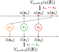
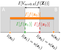
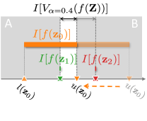
Assume that there exists such that and such that . Lemma 2 implies that with high probability. Hence, we may naïvely want to query for observations at and to reduce . However, these observations may not always reduce . The insight is that changes (i.e., shrinks) when either of its boundary values (i.e., or ) changes. Consider and finite as an example, since , a natural cause for the change in is when changes. This happens if there exists such that the ordering of relative to changes given more observations. Thus, observations that are capable of reducing should be able to change the relative ordering in this case. We construct the following counterexample where observations at (and ) are not able to change the relative ordering, so they do not reduce .
Example 1.
This example is described by Fig. 1. We reduce notational clutter by removing and since they are fixed in this example, i.e., we use , , and to denote , , and respectively. We condition on the event for all which occurs with probability in Lemma 3. In this example, and , so there is no uncertainty in . Similarly, there is no uncertainty in . Thus, new observations at and change neither nor , so these observations do not reduce the confidence bound (plotted as the double-headed arrow in Fig. 1b). In fact, to reduce , we should gather new observations at which potentially change the ordering of relative to (which is without new observations). For example, after getting new observations at , if is improved to be in the white region between A and B ( in Fig. 1b changes to in Fig. 1c), then is reduced to because now . Thus, as the confidence bound is shortened with more and more observations at , the confidence bound reduces (the white region in Fig. 1 is ‘laced up’).
 |
 |
 |
| (a) | (b) | (c) |
In the next section, we define a property of in Example 1 and prove the existence of ’s with this property. Then, we prove that along with the optimistic selection of , the selection of such that it satisfies this property leads to a no-regret algorithm.
3.2 Lacing Value (LV) and the Query Selection Strategy for
We note that in Example 1, as long as the confidence bound of the function evaluation at contains the confidence bound of VaR, observations at can reduce the confidence bound of VaR. We name the values of satisfying this property as lacing values (LV):
Definition 1 (Lacing values).
Lacing values (LV) with respect to and are that satisfies , equivalently,
Recall that the support of is defined as the smallest closed subset of such that (e.g., is a finite subset of and ). The following theorem guarantees the existence of lacing values and is proved in Appendix C.
Theorem 1 (Existence of lacing values).
, , , there exists a lacing value in with respect to and .
Corollary 1.1.
Lacing values with respect to and are in where and .
As a special case, when , which means is an LV. Based on Theorem 1, we can always select as an LV w.r.t defined in Definition 1. This strategy for the selection of , together with the selection of (Section 3.1), completes our algorithm: VaR Upper Confidence Bound (V-UCB) (Algorithm 1).
Upper Bound on Regret. As a result of the selection strategies for and , our V-UCB algorithm enjoys the following upper bound on its instantaneous regret (proven in Appendix D):
Lemma 3.
By selecting as a maximizer of and selecting as an LV w.r.t , the instantaneous regret is upper-bounded by:
with probability for in Lemma 3.
Lemma 3, together with Lemma 5.4 from Srinivas et al. (2010), implies that the cumulative regret of our algorithm is bounded (Appendix E): where , and is the maximum information gain about that can be obtained from any set of observations. Srinivas et al. (2010) have analyzed for several commonly used kernels such as SE and Matérn kernels, and have shown that for these kernels, the upper bound on grows sub-linearly. This implies that our algorithm is no-regret because .
Inspired by Bogunovic et al. (2018), at the -th iteration of V-UCB, we can recommend as an estimate of the maximizer of , where . Then, the instantaneous regret is upper-bounded by with high probability as we show in Appendix F. In our experiments in Section 4, we recommend (where is a random function defined in the same manner as ) as an estimate of due to its empirical convergence.
Computational Complexity. To compare our computational complexity with that of the algorithm from Cakmak et al. (2020), we exclude the common part of training the GP model (line 6) and assume that is finite. Then, the time complexity of V-UCB is dominated by that of the selection of (line 3) which includes the time complexity for the GP prediction at , and for the sorting of and searching of VaR. Hence, our overall complexity is , where is the number of iterations to maximize (line 3). Therefore, our V-UCB is more computationally efficient than and its variant with approximation , whose complexities are of and , respectively.222 and are the numbers of iterations for the outer and inner optimization respectively, is the number of fantasy GP models required for their one-step lookahead, and is the number of functions sampled from the GP posterior (Cakmak et al., 2020).
3.3 On the Selection of
Although Algorithm 1 is guaranteed to be no-regret with any choice of LV as , we would like to select the LV that can reduce a large amount of the uncertainty of . However, relying on the information gain measure or the knowledge gradient method often incurs the expensive one-step lookahead. Therefore, we use a simple heuristic by choosing the LV with the maximum probability mass (or probability density if is continuous) of . We motivate this heuristic using an example with , i.e., . Suppose is finite and there are LV’s and with and . Then, because , it follows that , i.e., querying at gives us information about an explicit upper bound on to reduce its uncertainty. In contrast, this cannot be achieved by querying due to its low probability mass. This simple heuristic can also be implemented when is a continuous random variable which we will introduce in Section 3.5.
Remark 1.
Although we assume that we can select both and during our algorithm, Corollary 1.1 also gives us some insights about the scenario where we cannot select . In this case, in each iteration , we select while is randomly sampled by the environment following the distribution of . Next, we observe both and and then update the GP posterior belief of . Of note, Corollary 1.1 has shown that all LV lie in the set . However, the probability of this set is usually small, because and small values of are often used by real-world applications to manage risks. Thus, the probability that the sampled is an LV is small. As a result, we suggest sampling a large number of ’s from the environment to increase the chance that an LV is sampled. On the other hand, the small probability of sampling an LV motivates the need for us to select .
3.4 V-UCB Approaches StableOpt as
Recall that the objective of adversarially robust BO is to find that maximizes (Bogunovic et al., 2018) by iteratively specifying input query to collect noisy observations . It is different from BO of VaR since its is not random but selected by an adversary who aims to minimize the function evaluation. The work of Bogunovic et al. (2018) has proposed a no-regret algorithm for this setting named StableOpt, which selects
| (5) |
where and are defined in (3).
At first glance, BO of VaR and adversarially robust BO are seemingly different problems because is a random variable in the former but not in the latter. However, based on our key observation on the connection between the minimum value of a continuous function and the VaR of the random variable in the following theorem, these two problems and their solutions are connected as shown in Corollary 2.1, and 2.2.
Theorem 2.
Let be a random variable with the support and dimension . Let be a continuous function mapping from to . Then, denotes the random variable whose realization is the function evaluation at a realization of . Suppose has a minimizer , then
Corollary 2.1.
Adversarially robust BO which finds can be cast as BO of VaR by letting (a) approach from the right and (b) be the support of the environmental random variable , i.e., .
Interestingly, from Theorem 2, we observe that in Corollary 1.1 approaches the set of minimizers as . Corollary 2.2 below shows that LV w.r.t becomes a minimizer of which is same as the selected of StableOpt in (5).
Corollary 2.2.
The StableOpt solution to adversarially robust BO selects the same input query as that selected by the V-UCB solution to the corresponding BO of VaR in Corollary 2.1.
The proof of Theorem 2 and its two corollaries are shown in Appendix G. We note that V-UCB is also applicable to the optimization of where the distribution of is a conditional distribution given . For example, in robotics, if there exists noise/perturbation in the control, an optimization problem of interest is where is the random perturbation that depends on .
3.5 Implementation of V-UCB with Continuous Random Variable
The V-UCB algorithm involves two steps: selecting and selecting as the LV with the largest probability mass (or probability density). When is finite, given , can be computed exactly. The gradient of with respect to can be obtained easily (e.g., using automatic differentiation provided in the Tensorflow library (Abadi et al., 2015)) to aid the selection of . In this case, the latter step can also be performed by constructing the set of all LV (checking the condition in the Definition 1 for all ) and choosing the LV with the largest probability mass.
Estimation of VaR. When is a continuous random variable, estimating VaR by an ordered set of samples (e.g., in Cakmak et al. (2020)) may require a prohibitively large number of samples, especially for small values of . Thus, we employ the following popular pinball (or tilted absolute value) function in quantile regression (Koenker & Bassett, 1978) to estimate VaR as a lower -quantile:
where . In particular, to estimate as , we find that minimizes:
| (6) |
A well-known example is when and is the absolute value function, then the optimal is the median. The loss in (6) can be optimized using stochastic gradient descent with a random batch of samples of at each optimization iteration.
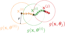
Maximization of . Unfortunately, to maximize over , there is no gradient of with respect to under the above approach. This situation resembles BO where there is no gradient information, but only noisy observations at input queries. Unlike BO, the observation (samples of at ) is not costly. Therefore, we propose the local neural surrogate optimization (LNSO) algorithm to find which is visualized in Fig. 2. Suppose the optimization is initialized at , instead of maximizing (whose gradient w.r.t. is unknown), we maximize a surrogate function (modeled by a neural network) that approximates well in a local region of , e.g., a ball of radius in Fig. 2. We obtain such parameters by minimizing the following loss function:
| (7) |
where the expectation is taken over a uniformly distributed in . Minimizing (7) can be performed with stochastic gradient descent. If maximizing leads to a value (Fig. 2), we update the local region to be centered at () and find such that approximates well . Then, is updated by maximizing for . The complete algorithm is described in Appendix H.
We prefer a small value of so that the ball is small. In such case, for can be estimated well with a small neural network whose training requires a small number of iterations.
Search of Lacing Values. Given a continuous random variable , to find an LV w.r.t in line 4 of Algorithm 1, i.e., to find a satisfying and , we choose a that minimizes
| (8) |
where is the rectified linear unit function (). To include the heuristic in Section 3.3 which selects the LV with the highest probability density, we find that minimizes
where is defined in (8); is the probability density; and are indicator functions.
4 Experiments
In this section, we empirically evaluate the performance of V-UCB. The work of Cakmak et al. (2020) has motivated the use of the approximated variant of their algorithm over its original version by showing that achieves comparable empirical performances to while incurring much less computational cost. Furthermore, has been shown to significantly outperform other competing algorithms (Cakmak et al., 2020). Therefore, we choose as the main baseline to empirically compare with V-UCB. The experiments using is performed by adding new objective functions to the existing implementation of Cakmak et al. (2020) at https://github.com/saitcakmak/BoRisk.
Regarding V-UCB, when is finite and the distribution of is not uniform, we perform V-UCB by selecting as an LV at random, labeled as V-UCB Unif, and by selecting as the LV with the maximum probability mass, labeled as V-UCB Prob.
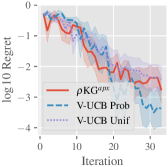
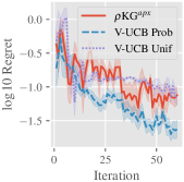
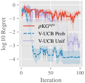
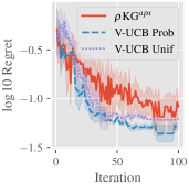
The performance metric is defined as where is the recommended input. The evaluation of VaR is described in Section 3.5. The recommended input is for V-UCB, and for (Cakmak et al., 2020), where is the conditional expectation over the unknown given the observations (approximated by a finite set of functions sampled from the GP posterior belief).333While the work of Cakmak et al. (2020) considers a minimization problem of VaR, our work considers a maximization problem of VaR. Therefore, the objective functions for are the negation of those for V-UCB. For V-UCB at risk level , the risk level for is . We repeat each experiment times with different random initial observations and plot both the mean (as lines) and the confidence interval (as shaded areas) of the of the performance metric. The detailed descriptions of experiments are deferred to Appendix I.
4.1 Synthetic Benchmark Functions
We use synthetic benchmark functions: Branin-Hoo, Goldstein-Price, and Hartmann-3D functions to construct optimization problems: Branin-Hoo-, Goldstein-Price-, Hartmann-, and Hartmann-. The tuples represent corresponding to the dimensions of and . The noise variance is set to . The risk level is . There are different settings: finite ( for Hartmann- and for the others) and continuous . In the latter setting, and the surrogate function is a neural network of hidden layers with hidden neurons each, and sigmoid activation functions.
The results are shown in Fig. 3 and Fig. 4 for the settings of discrete and continuous , respectively. When is discrete (Fig. 3), V-UCB Unif is on par with in optimizing Branin-Hoo- and Goldstein-Price-, and outperforms in optimizing Hartmann- and Hartmann-. V-UCB Prob is also able to exploit the probability distribution of to outperform V-UCB Unif. When is continuous (Fig. 4), V-UCB Prob outperforms . The unsatisfactory performance of in some experiments may be attributed to its approximation of the inner optimization problem in the acquisition function (Cakmak et al., 2020), and the approximation of VaR using samples of and the GP posterior belief.
 |
 |
| (a) Branin-Hoo- | (b) Goldstein-Price- |
 |
 |
| (c) Hartmann- | (d) Hartmann- |
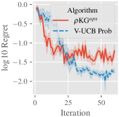 |
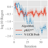 |
| (a) Branin-Hoo- | (b) Goldstein-Price- |
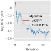 |
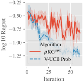 |
| (c) Hartmann- | (d) Hartmann- |
4.2 Simulated Optimization Problems
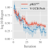
The first problem is portfolio optimization adopted by (Cakmak et al., 2020). There are optimization variables (risk and trade aversion parameters, and the holding cost multiplier) and environmental random variables (bid-ask spread and borrow cost). The variable follows a discrete uniform distribution with . Hence, there is no difference between V-UCB Unif and V-UCB Prob. Thus, we only report the results of the latter. The objective function is the posterior mean of a trained GP on the dataset in Cakmak et al. (2020) of size generated from CVXPortfolio. The noise variance is set to . The risk level is set to .
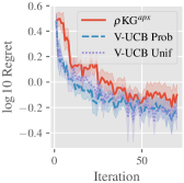
The second problem is a simulated robot pushing task for which we use the implementation from the work of Wang & Jegelka (2017). The simulation is viewed as a -dimensional function returning the 2-D location of the pushed object, where are the robot location and is the pushing duration. The objective is to minimize the distance to a fixed goal location , i.e., the objective function of the maximization problem is . We assume that there are perturbations in specifying the robot location whose support includes equi-distant points in and whose probability mass is proportional to . It leads to a random objective function . We aim to maximize the VaR of which is more difficult than maximizing that of . Moreover, a random noise following is added to the evaluation of . The risk level is set to .
The results are shown in Fig. 5. We observe that V-UCB outperforms in both problems. Furthermore, in comparison to our synthetic experiments, the difference between V-UCB Unif and V-UCB Prob is not significant in the robot pushing experiment. This is because the chance that a uniform sample of LV has a large probability mass is higher in the robot pushing experiment due to a larger region of having high probabilities.
 |
 |
| (a) Portfolio optimization | (b) Robot pushing |
5 Conclusion
To tackle the BO of VaR problem, we construct a no-regret algorithm, namely VaR upper confidence bound (V-UCB), through the design of a confidence bound of VaR and a set of lacing values (LV) that is guaranteed to exist. Besides, we introduce a heuristic to select an LV that improves the emprical performance of V-UCB over random selection of LV. We also draw an elegant connection between BO of VaR and adversarially robust BO in terms of both problem formulation and solutions. Lastly, we provide practical techniques for implementing VaR with continuous . While V-UCB is more computationally efficient than the the state-of-the-art algorithm for BO of VaR, it also demonstrates competitive empirical performances in our experiments.
References
- Abadi et al. (2015) Abadi, M., Agarwal, A., Barham, P., Brevdo, E., Chen, Z., Citro, C., Corrado, G. S., Davis, A., Dean, J., Devin, M., Ghemawat, S., Goodfellow, I., Harp, A., Irving, G., Isard, M., Jia, Y., Jozefowicz, R., Kaiser, L., Kudlur, M., Levenberg, J., Mané, D., Monga, R., Moore, S., Murray, D., Olah, C., Schuster, M., Shlens, J., Steiner, B., Sutskever, I., Talwar, K., Tucker, P., Vanhoucke, V., Vasudevan, V., Viégas, F., Vinyals, O., Warden, P., Wattenberg, M., Wicke, M., Yu, Y., and Zheng, X. TensorFlow: Large-scale machine learning on heterogeneous systems, 2015. URL https://www.tensorflow.org/. Software available from tensorflow.org.
- Basel Committee on Banking Supervision (2006) Basel Committee on Banking Supervision. International convergence of capital measurement and capital standards, 2006. URL http://www.bis.org/publ/bcbs22.pdf.
- Bogunovic et al. (2016) Bogunovic, I., Scarlett, J., Krause, A., and Cevher, V. Truncated variance reduction: A unified approach to bayesian optimization and level-set estimation. In Proc. NIPS, pp. 1507–1515, 2016.
- Bogunovic et al. (2018) Bogunovic, I., Scarlett, J., Jegelka, S., and Cevher, V. Adversarially robust optimization with Gaussian processes. In Proc. NeurIPS, pp. 5760–5770, 2018.
- Cakmak et al. (2020) Cakmak, S., Astudillo, R., Frazier, P. I., and Zhou, E. Bayesian optimization of risk measures. In Proc. NeurIPS, 2020.
- Chowdhury & Gopalan (2017) Chowdhury, S. R. and Gopalan, A. On kernelized multi-armed bandits. In Proc. ICML, pp. 844–853, 2017.
- Goh et al. (2012) Goh, J. W., Lim, K. G., Sim, M., and Zhang, W. Portfolio value-at-risk optimization for asymmetrically distributed asset returns. European Journal of Operational Research, 221(2):397–406, 2012.
- Iwazaki et al. (2020) Iwazaki, S., Inatsu, Y., and Takeuchi, I. Mean-variance analysis in Bayesian optimization under uncertainty. arXiv preprint arXiv:2009.08166, 2020.
- Kirschner et al. (2020) Kirschner, J., Bogunovic, I., Jegelka, S., and Krause, A. Distributionally robust Bayesian optimization. In Proc. AISTATS, 2020.
- Koenker & Bassett (1978) Koenker, R. and Bassett, G. Regression quantiles. Econometrica: Journal of the econometric society, pp. 33–50, 1978.
- Nguyen et al. (2020) Nguyen, T. T., Gupta, S., Ha, H., Rana, S., and Venkatesh, S. Distributionally robust Bayesian quadrature optimization. In Proc. AISTATS, 2020.
- Rasmussen & Williams (2006) Rasmussen, C. E. and Williams, C. K. I. Gaussian processes for machine learning. MIT Press, 2006.
- Scott et al. (2011) Scott, W., Frazier, P., and Powell, W. The correlated knowledge gradient for simulation optimization of continuous parameters using Gaussian process regression. SIAM journal on optimization, 21(3):996–1026, 2011.
- Srinivas et al. (2010) Srinivas, N., Krause, A., Kakade, S., and Seeger, M. Gaussian process optimization in the bandit setting: No regret and experimental design. In Proc. ICML, pp. 1015–1022, 2010.
- Torossian et al. (2020) Torossian, L., Picheny, V., and Durrande, N. Bayesian quantile and expectile optimisation. arXiv preprint arXiv:2001.04833, 2020.
- Toscano-Palmerin & Frazier (2018) Toscano-Palmerin, S. and Frazier, P. I. Bayesian optimization with expensive integrands. arXiv preprint arXiv:1803.08661, 2018.
- Wang & Jegelka (2017) Wang, Z. and Jegelka, S. Max-value entropy search for efficient Bayesian optimization. In Proc. ICML, pp. 3627–3635, 2017.
- Williams et al. (2000) Williams, B. J., Santner, T. J., and Notz, W. I. Sequential design of computer experiments to minimize integrated response functions. Statistica Sinica, pp. 1133–1152, 2000.
Appendix A Proof of Lemma 2
Lemma 2. Similar to the definition of , let and denote the random function over where the randomness comes from the random variable ; and are defined in (3). Then, , , ,
holds with probability for in Lemma 3, where and are defined as (1).
Proof.
Conditioned on the event for all , , which occurs with probability for in Lemma 3, we will prove that . The proof of can be done in a similar manner.
From for all , , we have
Therefore, for all , , , ,
So, for all , , , ,
Hence, the set is a subset of for all , , , which implies that , i.e., for all , , . ∎
Appendix B Proof of (4)
Appendix C Proof of Theorem 1
Theorem 1. , , , there exists a lacing value in with respect to and .
Proof.
Recall that
From to the definition of and , we have
| (10) |
Since , . We prove the existence of LV by contradiction: (a) assuming that and then, (b) proving that is not a lower bound of which is a contradiction.
Since the GP posterior mean and posterior standard deviation are continuous functions in , and are continuous functions in the closed ( and are given and remain fixed in this proof). We will prove that is closed in by contradiction.
If is not closed in , there exists a limit point of such that . Since and is closed in , . Thus, for , (from the definition of ). Then, there exists such that . The pre-image of the open interval under is also an open set containing (because is a continuous function). Since is a limit point of , there exists an . Then, , so . It contradicts .
Therefore, is a closed set in . Besides, since is upper bounded by (due to our assumption), so exists. Let be such that . Then, because is closed.
Moreover, from our assumption that , we have . Furthermore,
where the first inequality is because and the last inequality is from (10). Hence, is not a lower bound of . ∎
Appendix D Proof of Lemma 3
Appendix E Bound on the Average Cumulative Regret
Appendix F Bound on
Conditioned on the event for all , , , which occurs with probability in Lemma 3, it follows that for all in Lemma 2. Furthermore, we select as an LV, so according to the Definition 1.
At -th iteration, by recommending as an estimate of where , we have
Therefore,
Furthermore, from our condition, so
Since is shown to be bounded for several common kernels in (Srinivas et al., 2010), the above implies that .
Appendix G Proof of Theorem 2 and Its Corollaries
G.1 Proof of Theorem 2
Theorem 2. Let be a random variable with the support and dimension . Let be a continuous function mapping from to . Then, denotes the random variable whose realization is the function evaluation at a realization of . Suppose has a minimizer , then
Recall that the support of is defined as the smallest closed subset of such that , and minimizes .
Lemma 4.
For all , is a nondecreasing function, i.e.,
Proof.
Since , for all ,
Therefore, is a subset of . Thus,
i.e., ∎
Lemma 5.
For all , and defined in (12)
We use Lemma 5 to prove the following lemma.
Lemma 6.
Proof.
By contradiction, we assume that there exits such that . Then, there exists such that . Consider the pre-image of the open interval . Since is a continuous function, is an open set and it contains (as contains ). Then, consider the set , we prove by contradiction as follows.
If then the closure of is a closed set that is smaller than (since is an open set, is a closed set, and is not empty) and satisfies , which contradicts the definition of . Thus, .
Lemma 7.
For defined in (12)
| (13) |
Proof.
By contradiction, we assume that . Then there exists that . Since so there exits such that . However,
which contradicts the fact that . Therefore, . ∎
G.2 Corollary 2.2
From Theorem 2, is a closed subset of , and , are continuous functions over , it follows that the selected by both StableOpt (in (5)) and V-UCB are the same. Furthermore,
Therefore, the set of lacing values is any of which is also the selected in (5) by StableOpt. Thus, the selected by both StableOpt and V-UCB are the same.
Appendix H Local Neural Surrogate Optimization
The local neural surrogate optimization (LNSO) to maximize a VaR is described in Algorithm 2. The algorithm can be summarized as follows:
-
•
Whenever the current updated is not in (line 4), the center of the ball is updated to be (line 6) and the surrogate function is re-trained (lines 7-12).
-
•
The surrogate function is (re-)trained to estimate well for all (lines 7-12) with stochastic gradient descent by minimizing the following loss function given random mini-batches of (line 8) and of (line 9):
(14) where is the pinball function in Sec. 3.5.
-
•
Instead of directly maximizing whose gradient w.r.t is unavailable, we find that maximizes the surrogate function (line 14) where is the parameters trained in lines 7-12.
Appendix I Experimental Details
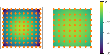
Regarding the construction of in optimizing the synthetic benchmark functions, the discrete is selected as equi-distanct points (e.g., by dividing into a grid). The probability mass of is defined as (the subtraction is elementwise). The continuous follows a -standard-deviation truncated independent Gaussian distribution with the mean of and standard deviation . It is noted that when is discrete, there is a large region of with low probability in experiments with synthetic benchmark functions. This is to highlight the advantage of V-UCB Prob in exploiting compared with V-UCB Unif. In the robot pushing experiment, the region of with low probability is smaller than that in the experiments with synthetic benchmark functions (e.g., Hartmann-), which is illustrated in Fig. 6. Therefore, the gap in the performance between V-UCB Unif and V-UCB Prob is smaller in the robot pushing pushing experiment (Fig. 5b) than that in the experiment with Hartmann- (Fig. 3c).
When the closed-form expression of the objective function is known (e.g., synthetic benchmark functions) in the evaluation of the performance metric, the maximum value can be evaluated accurately. On the other hand, when the closed-form expression of the objective function is unknown even in the evaluation of the performance metric (e.g., the simulated robot pushing experiment), the maximum value is estimated by where are input queries in the experiments with both V-UCB and . The addition of is to avoid value in plots of the log values of the performance metric.
The sizes of the initial observations are for the Branin-Hoo and Goldstein-Price functions; for the Hartmann-3D function; for the portfolio optimization problem; and for the simulated robot pushing task. The initial observations are randomly sampled for different random repetitions of the experiments, but they are the same between the same iterations in V-UCB and .
The hyperparameters of GP (i.e., the length-scales and signal variance of the SE kernel) and the noise variance are estimated by maximum likelihood estimation (Rasmussen & Williams, 2006) every iterations of BO. We set a lower bound of for the noise variance to avoid numerical errors.
To show the advantage of LNSO, we set the number of samples of to be for both V-UCB and . The number of samples of , i.e., , in LNSO (line 9 of Algorithm 2) is . The radius of the local region is set to be a small value of such that a small neural network works well: hidden layers with hidden neurons at each layer; the activation functions of the hidden layers and the output layer are sigmoid and linear functions, respectively.
Since the theoretical value of is often considered as excessively conservative (Bogunovic et al., 2016; Srinivas et al., 2010; Bogunovic et al., 2018). We set in our experiments while can be tuned to achieved better exploration-exploitation trade-off (Srinivas et al., 2010) or multiple values of can be used in a batch mode (Torossian et al., 2020).