Interstellar Gas Heating by Primordial Black Holes

Abstract

Interstellar gas heating is a powerful cosmology-independent observable for exploring the parameter space of primordial black holes (PBHs) formed in the early Universe that could constitute part of the dark matter (DM). We provide a detailed analysis of the various aspects for this observable, such as PBH emission mechanisms. Using observational data from the Leo T dwarf galaxy, we constrain the PBH abundance over a broad mass-range, $M_{\rm PBH}\sim\mathcal{O}(1)M_{\odot}-10^{7}M_{\odot}$, relevant for the recently detected gravitational wave signals from intermediate-mass BHs. We also consider PBH gas heating of systems with bulk relative velocity with respect to the DM, such as Galactic clouds.

1 Introduction

Primordial black holes (PBHs) can form in the early Universe, prior to galaxies and stars, through a variety of mechanisms and can constitute a significant fraction of the dark matter (DM) (e.g. Zeldovich:1967 ; Hawking:1971ei ; Carr:1974nx ; Khlopov:1980mg ; Khlopov:1985jw ; Kawasaki:1997ju ; GarciaBellido:1996qt ; Khlopov:2008qy ; Frampton:2010sw ; Kawasaki:2016pql ; Carr:2016drx ; Inomata:2016rbd ; Pi:2017gih ; Inomata:2017okj ; Garcia-Bellido:2017aan ; Georg:2017mqk ; Inomata:2017vxo ; Kocsis:2017yty ; Ando:2017veq ; Cotner:2016cvr ; Cotner:2017tir ; Cotner:2018vug ; Sasaki:2018dmp ; Carr:2018rid ; Banik:2018tyb ; 1939PCPS…35..405H ; Cotner:2019ykd ; Kusenko:2020pcg ; Flores:2020drq ; Domenech:2021uyx ). Depending on the formation mechanism, the PBH mass can span many orders of magnitude. Those PBHs with mass above $M\gtrsim 10^{15}$ g survive Hawking evaporation until present. In a sizable mass range, $M\sim 10^{-16}-10^{-10}M_{\odot}$, PBHs can constitute all of the DM Katz:2018zrn ; Smyth:2019whb ; Montero-Camacho:2019jte ; Sugiyama:2019dgt ; Niikura:2017zjd . PBHs have been associated with a variety of astrophysical phenomena and puzzles, e.g. PBHs could be the seeds for the formation of super-massive black holes (e.g. Bean:2002kx ; Kawasaki:2012kn ; Clesse:2015wea ) and could lead to new signatures from compact star disruptions from PBH capture (e.g. Fuller:2017uyd ; Takhistov:2017nmt ; Takhistov:2017bpt ; Takhistov:2020vxs ).

PBHs in the mass window of $\sim 10-10^{3}M_{\odot}$ have been suggested as progenitors Nakamura:1997sm ; Clesse:2015wea ; Bird:2016dcv ; Raidal:2017mfl ; Eroshenko:2016hmn ; Sasaki:2016jop ; Clesse:2016ajp for the gravitational wave (GW) signals detected by LIGO (e.g. Abbott:2016blz ; Abbott:2016nmj ; Abbott:2017vtc ). The first definitive observation of intermediate-mass $150M_{\odot}$ BH has been claimed by LIGO (Abbott:2020tfl, ). In conventional stellar evolution astrophysics such BHs are difficult to form from the collapse of a single star, akin to the formation of stellar-mass BHs. While this PBH DM parameter space region is already under pressure from a variety of constraints (see Ref. (Carr:2020gox, ) for review), these rely on and are sensitive to uncertainties of underlying assumptions, which often include the cosmological history.

In Ref. Lu:2020bmd we have put forth a novel cosmology-independent observable, based on PBHs heating of the surrounding interstellar medium (ISM) gas, as a powerful probe for stellar and intermediate-mass PBHs contributing to the DM. In this work we further explore this observable and provide a detailed analysis of PBH gas heating as well as various underlying processes, such as PBH emission mechanisms. Following Ref. Lu:2020bmd , we focus on the Leo T irregular dwarf galaxy as a particularly favorable astrophysical system target. Further, we extend the analysis to include systems with bulk velocity relative to the DM.

The “heating” of near-by stars by passing massive BHs has been previously considered Carr:1999dyn ; Lacey:1985 ; Totani:2010 . Theoretically expected X-ray emission from traversing PBHs interacting with the surrounding medium has been also employed to set limits on the PBH DM fraction Gaggero:2016dpq ; Inoue:2017csr ; Hektor:2018rul . Constraints from gas heating and system cooling have been considered in the context of particle DM candidates Bhoonah:2018wmw ; Farrar:2019qrv ; Wadekar:2019mpc , which however have heating mechanisms different from PBHs. Further, while the focus for particle DM is on target astrophysical systems with high relative particle velocities resulting in high collision rates, for PBHs the astrophysical systems with slower relative velocities are favored due to increased PBH accretion and resulting emission.

While our discussion focuses on present-day effects, emission from gas-accreting PBHs is also relevant for cosmology, e.g. for the reionization and recombination epochs (e.g. Ricotti:2007au ). X-ray emission from gas accreting onto PBHs would result in ionization and increased quantities of molecular hydrogen, which would in turn provide cooling and enhance earlier star formation Ricotti:2007au . Further, emission from accreting PBHs could result in spectral $\mu-$ and $y-$distortions of the cosmic microwave background (CMB). Heating and ionization of intergalactic medium gas from PBH emission could modify 21cm power spectrum in an observable way Hektor:2018qqw ; Mena:2019nhm . In this work we do not discuss cosmological effects, which provide complementary ways of exploring PBH DM.

2 PBHs in ISM

2.1 Bondi-Hoyle-Lyttleton accretion

X-ray emission from gas-accreting isolated BHs traversing the ISM of the Milky Way was explored in Ref. Agol:2001hb . Ref. Inoue:2017csr adapted the analysis for PBHs constituting part of the DM. In this section we broadly follow the same method. PBHs traveling at low Mach number $\mathcal{M}=v/c_{s}$ accrete via the Bondi-Hoyle-Lyttleton process, with an accretion rate 1939PCPS…35..405H ; 1944MNRAS.104..273B ; 1952MNRAS.112..195B

$$\dot{M}=4\pi r_{B}^{2}\tilde{v}\rho=\frac{4\pi G^{2}M^{2}n\mu m_{p}}{\tilde{v}^{3}}~{}.$$ (1)

Here $M$ is the PBH mass, $r_{B}=GM/\tilde{v}^{2}$ is the Bondi radius, $\mu$ is the mean molecular weight, $n$ is the ISM gas number density, $m_{p}$ is the proton mass and $\tilde{v}\equiv(v^{2}+c_{s}^{2})^{1/2}$, where $v$ is the PBH velocity relative to the ISM gas and $c_{s}$ is the temperature-dependent sound speed in gas, which we take to be approximately $c_{s}\sim 10$ km/s Inoue:2017csr . At high Mach number, the BH accretion rate is expected to be limited to $\sim 10$–$20$% of the canonical Bondi-Hoyle-Lyttleton accretion rate of Eq. (1) Guo:2020qkf , as shown by recent 3D hydrodynamical simulations. However, the resulting system behavior is sensitive to assumed initial conditions. We find that it is the low-velocity regime that predominantly contributes to our effects of interest. Hence, we adopt the standard accretion rate of Eq. (1).

The bolometric luminosity of the accretion disk of a BH can be related to its accretion rate as $L=\epsilon(\dot{M})\dot{M}$. Here $\epsilon(\dot{M})$ is an effective phenomenological parameter describing radiative efficiency, which varies according to different accretion regimes. Assuming a radiative efficiency of $\epsilon_{0}=0.1$ characteristic of thin disks, the Eddington accretion rate in terms of Eddington luminosity is

$$\dot{M}_{\textrm{Edd}}=\frac{L_{\textrm{Edd}}}{\epsilon_{0}c^{2}}=6.7\times 10^{-16}\left(\frac{M}{M_{\odot}}\right)~{}M_{\odot}\text{/s}~{}.$$ (2)

To determine the accretion regimes of interest, it is useful to introduce a dimensionless form of the accretion rate

$$\dot{m}=\frac{\dot{M}}{\dot{M}_{\textrm{Edd}}}=2.64\times 10^{-7}\left(\frac{M}{M_{\odot}}\right)\left(\frac{n}{1\textrm{ cm}^{-3}}\right)\left(\dfrac{\mu}{1}\right)\left(\frac{\tilde{v}}{10\textrm{ km}/\textrm{s}}\right)^{-3}~{}.$$ (3)

2.2 Accretion disk formation

An accretion disk can form around a BH from the gas infalling with sufficient angular momentum. For accretion rates $\dot{m}\gtrsim 0.07\alpha$, a standard thin $\alpha$-disk Shakura:1972te likely forms. Here the disk’s viscosity is described by a phenomenological parameter $\alpha\sim\mathcal{O}(0.1)$. Perturbations in the density or velocity distributions of the surrounding gas can supply angular momentum to the disk. Assuming a Kolmogorov spectrum of density fluctuations in the ISM, the resulting density differential on opposing sides of the accretion “cylinder” can be calculated 1976ApJ…204..555S . We equate the angular momentum from this differential with the angular momentum of the outer edge of the thin disk Agol:2001hb ,

$$r_{\rm out}\simeq 5.4\times 10^{9}r_{s}\left(\frac{M}{100M_{\odot}}\right)^{\frac{2}{3}}\left(\frac{\tilde{v}}{10\textrm{ km/s}}\right)^{-\frac{10}{3}}~{},$$ (4)

where $r_{s}=2GM/c^{2}$ is the BH Schwarzschild radius. On the other hand, for inefficient accretion described by the Advection-Dominated Accretion Flow (ADAF) regime Narayan:1994xi ; Yuan:2014gma , the inflowing matter does not follow a Keplerian description. In this case, the outer accretion disk radius is uncertain and we consider a range of parameter values as described in Sec. 3.

The inner edge of the accretion disk is assumed to follow the innermost stable circular orbit (ISCO) of a test particle, which for a Schwarzschild BH is $r_{\rm ISCO}=3r_{s}$. If the outer edge of the BH accretion disk, at $r_{\rm out}$, is found to be located within the ISCO radius, i.e. $r_{\rm out}/r_{\rm ISCO}<1$, we do not expect efficient disk formation. Thus, using Eq. (4) we can infer an approximate condition on the mass of a BH for accretion disk formation as

$$M>2.5\times 10^{-13}M_{\odot}\left(\frac{\tilde{v}}{10\textrm{ km/s}}\right)^{5}~{}.$$ (5)

This condition is well-satisfied for all BHs in our parameter range of interest. On the other hand, it shows that small PBHs are generally not expected to have an accretion disk.

2.3 Gas and PBH distributions

The total number of PBHs of mass $M$ within a gas system of volume $V$ and DM density $\rho_{\rm DM}$, assuming PBHs make up a fraction $f_{\rm PBH}$ of the DM, is given by

$$N_{\rm PBH}(M)=f_{\rm PBH}\frac{\rho_{\rm DM}V}{M}~{}.$$ (6)

Our considerations apply in case there is at least one PBH in the gas system. This results in a lower “incredulity” limit

$$f_{\textrm{bound}}>\frac{3M}{4\pi r_{\textrm{sys}}^{3}\rho_{\textrm{DM}}}~{},$$ (7)

where $r_{\textrm{sys}}$ is the size of the system.

Here we assume a monochromatic PBH mass function, however our results can be readily applied to an extended PBH mass distribution. The velocity of PBHs contributing to the DM can be described by a Maxwell-Boltzmann distribution

$$\frac{df_{v}}{dv}(v)=\sqrt{\frac{2}{\pi}}\frac{v^{2}}{\sigma_{v}^{3}}\exp\left(-\frac{v^{2}}{2\sigma_{v}^{2}}\right)~{},$$ (8)

where $\sigma_{v}$ is the velocity dispersion within a given system.

We are interested in the gas heating due to PBHs. For a gas system in thermal equilibrium, we estimate the total amount of heating $H_{\rm tot}$ from PBHs of mass $M$ as

$$H_{\rm tot}(M)=N_{\rm PBH}(M)H(M)\simeq N_{\rm PBH}(M)\int_{n_{\textrm{min}}}^{n_{\textrm{max}}}\int_{v_{\textrm{min}}}^{v_{\textrm{max}}}dndv\frac{df_{n}}{dn}\frac{df_{v}}{dv}\mathcal{H}(M,n,v)~{},$$ (9)

where $df_{n}/dn$ is the gas number density distribution, $df_{v}/dv$ is the relative PBH velocity distribution and $\mathcal{H}(M,n,v)$ is the amount of heat being deposited into the system from a single PBH and also takes into account other potential contributing effects (e.g. photon absorption). $\mathcal{H}$ represents the cumulative contribution of all three heating mechanisms we consider below. For photon emission as well as outflows, there is an additional integration to treat absorption. For the gas systems of interest the density is approximately constant, for which $df_{n}/dn$ can be taken as a delta function in $n$.

3 Gas Heating Mechanisms

We consider three distinct gas heating mechanisms due to PBHs: absorption of photons emitted from the accretion disk, direct heating due to dynamical friction and energy deposit by protons of outflows that are inherent to the ADAF regime. Of these three, dynamical friction has the least uncertainty but typically constitutes a subdominant contribution. Since for our relevant parameters of interest the PBHs are in the stellar and intermediate-mass BH-range, the heating associated with Hawking evaporation is negligible. Following the original proposal of Ref. Lu:2020bmd , PBH gas heating has been recently considered in the context of small evaporating PBHs as well Kim:2020ngi ; Laha:2020vhg .

3.1 Accretion photon emission

Photon emission from PBH accretion disks is one of the major contributors to the ISM gas heating. Emission in the X-ray band is most readily absorbed by the surrounding hydrogen ISM gas, becoming efficient when the mass accretion rates are significant.

For different accretion disk regimes we follow Ref. Yuan:2014gma . We consider that the accretion flow results in a thin disk formation when $\dot{m}>\dot{M}=0.07\alpha$, and is described by ADAF for less efficient accretion. We do not consider the “slim disk” and other solutions relevant for near-Eddington or super-Eddington accretion when $\dot{m}\sim 1$, as the PBHs in our parameter space of interest are not expected to typically achieve such high rates. Furthermore, the slim disk emission spectrum is not significantly different from the spectrum of the thin disk for $\dot{m}\lesssim 10$ 1999ApJ…522..839W . In Fig. 1, we display the primary photon emission band from accreting PBHs over a wide range of PBH masses and for different densities of the surrounding gas, assuming Bondi-Hoyle-Lyttleton accretion of Eq. 1 with a characteristic flow velocity of $\tilde{v}\simeq 10$ km/s, and emission results of Sec. 3.1.1 and Sec. 3.1.2. Fig. 1 suggests which PBH observational signatures could be generically expected for a particular environment. In certain accretion regimes the disk size could grow to become comparable to the Bondi radius and feedback effects on the accretion can appear. However, we expect that PBHs can still efficiently accrete, e.g. from outside the plane of the disk. Throughout we assume that Bondi accretion continues to hold.

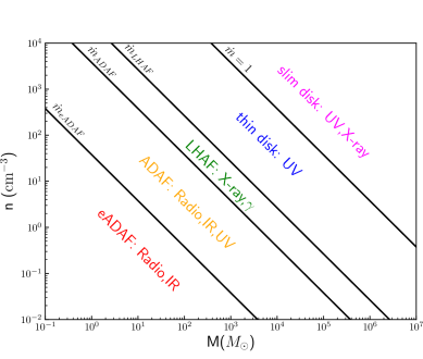
Figure 1: Dominant photon emission from PBH accretion over a wide mass-range of PBHs $M$, for different number densities $n$ of the surrounding gas, assuming Bondi-Hoyle-Lyttleton accretion and a characteristic flow velocity of $\tilde{v}\simeq 10$ km/s in Eq. (1). Regions of different accretion regimes $\dot{m}$ (black diagonal lines) resulting in slim disk, thin disk and ADAF (including LHAF, ADAF, eADAF sub-regimes, see text) accretion flows are shown.

Hydrogen gas absorbs ionizing radiation efficiently, but below the threshold of $E_{i}=13.6~{}\textrm{eV}$, hydrogen is optically thin to continuous emission. For non-relativistic gas velocity dispersions, Doppler broadening of the emission spectra is not significant so that we can ignore scattering with photons that have energies lower than $E_{i}$. The majority of photons are absorbed and a significant fraction of the energy is deposited as heat when the medium is optically thick. For $13.6\textrm{ eV}<E<30\textrm{ eV}$, we employ the photo-ionization cross-section of Refs. Bethe1957 ; 1990A&A…237..267B ,

$$\sigma(E)=\sigma_{0}y^{-\frac{3}{2}}\left(1+y^{\frac{1}{2}}\right)^{-4}~{},$$ (10)

where $y=E/E_{0}$, $E_{0}=1/2E_{i}$ and $\sigma_{0}=605.73\textrm{ Mb}=6.06\times 10^{-16}\textrm{ cm}^{2}$. The optical depth for a gas system of size $l$ and number density $n$ is then given by

$$\tau(n,E)=\sigma(E)nl~{}.$$ (11)

Above $30\textrm{ eV}$, we use attenuation length data from Fig. (32.16) of Ref. Olive_2014 .

The resulting heating power due to accretion disk emission photons is

$$\mathcal{H}(M,n,v)=\int_{E_{i}}^{E_{\textrm{max}}}L_{\nu}(M,n,v)f_{h}\left(1-e^{-\tau}\right)d\nu~{},$$ (12)

where $L_{\nu}(\nu)$ is the photon luminosity at frequency $\nu$ and $f_{h}$ is the fraction of energy deposited as heat that we estimate to be $\sim 1/3$ 1985ApJ…298..268S ; Ricotti:2001zf ; Furlanetto:2009uf ; Kim:2020ngi . Both the ADAF and thin disk emission spectra decrease exponentially at high energies, so we evaluate the integral up to a maximum energy $E_{\rm max}$, above which the contributions are negligible.

3.1.1   Thin disks

The standard (geometrically) thin $\alpha$-disk, characterized by the viscosity parameter $\alpha$, is optically thick and efficiently emits blackbody radiation Shakura:1972te . Thin disk allows for a fully analytic description. The temperature of the disk varies with radius as Pringle:1981ds

$$T(r)=T_{i}\left(\frac{r_{i}}{r}\right)^{3/4}\left[1-\left(\frac{r_{i}}{r}\right)^{\frac{1}{2}}\right]^{\frac{1}{4}}~{},$$ (13)

where $r_{i}$ is the inner disk radius taken to be the ISCO radius $r_{\rm ISCO}=3r_{s}$ as before. Here, using Eq. (1),

$$T_{i}=\left(\frac{3GM\dot{M}}{8\pi r_{i}^{3}\sigma_{B}}\right)^{1/4}=53.3\textrm{ eV}\left(\frac{n}{1\textrm{ cm}^{-3}}\right)^{\frac{1}{4}}\left(\frac{\tilde{v}}{10\textrm{ km}/\textrm{s}}\right)^{-\frac{3}{4}}~{},$$ (14)

where $\sigma_{B}$ is the Stefan-Boltzmann constant. For Bondi-Hoyle-Lyttleton accretion, the disk temperature is seen to be independent of the BH mass. The disk temperature $T(r)$ decreases at large radii as $r^{-3/4}$, but also diminishes near the inner radius. The disk attains a maximum temperature of $T_{\rm max}=0.488T_{i}$ at a radius of $r=1.36r_{i}$.

The thin disk emission spectrum is a combined contribution of the blackbody spectra from each radius. Using the scaling relations in Ref. Pringle:1981ds and requiring continuity, the resulting spectrum can be approximately described as

$$\begin{split}\nu<T_{o}:~{}~{}~{}~{}~{}&L_{\nu}=c_{\alpha}\left(\frac{T_{\rm max}}{T_{o}}\right)^{\frac{5}{3}}\left(\frac{\nu}{T_{\textrm{max}}}\right)^{2}\\ T_{o}<\nu<T_{\rm max}:~{}~{}~{}~{}~{}&L_{\nu}=c_{\alpha}\left(\frac{\nu}{T_{\textrm{max}}}\right)^{\frac{1}{3}}\\ T_{\rm max}<\nu:~{}~{}~{}~{}~{}&L_{\nu}=c_{\alpha}\left(\frac{\nu}{T_{\textrm{max}}}\right)^{2}e^{1-\frac{\nu}{T_{\rm max}}}\end{split}$$ (15)

where

$$c_{\alpha}=1.27\times 10^{29}\textrm{ erg}\textrm{ eV}^{-1}\textrm{s}^{-1}\Big{(}\dfrac{M}{M_{\odot}}\Big{)}^{2}\Big{(}\dfrac{n}{1\textrm{ cm}^{-3}}\Big{)}^{3/4}\Big{(}\dfrac{\tilde{v}}{10\textrm{ km}/\textrm{s}}\Big{)}^{-9/4}~{}.$$ (16)

Here $c_{\alpha}$ is normalized so that the total integrated luminosity (power) is $\int L_{\nu}d\nu=0.057\dot{M}c^{2}$, i.e. emission has the maximum possible efficiency for a Schwarzschild black hole. Using Eq. (1), (4) and (13), the temperature at the outer disk radius $T_{o}=T(r_{\rm out})$ is given by

$$T_{o}\simeq 6.13\times 10^{-5}\textrm{ eV}\left(\frac{n}{1\textrm{ cm}^{-3}}\right)^{\frac{1}{4}}\left(\frac{M}{M_{\odot}}\right)^{-\frac{1}{2}}\left(\frac{\tilde{v}}{10\textrm{ km}/\textrm{s}}\right)^{\frac{7}{4}}~{}.$$ (17)

For all relevant parameter values of interest for $n,M,\tilde{v}$, the temperature is always $T_{o}\ll 13.6~{}\textrm{eV}$.

Eq. (14) shows that thin disks efficiently emit at X-ray frequencies, a regime where the hydrogen ionization cross section is large. Hence, the emission from thin disks would be well absorbed and could contribute significantly to gas heating.

3.1.2   ADAF - emission power

When the accretion is significantly sub-Eddington, ADAF disks form Narayan:1994xi ; Yuan:2014gma . Here, the heat generated by viscosity during accretion is not efficiently radiated out and much of the energy is advected via matter heat capture into the BH event horizon, along with the gas inflow. In contrast to the thin disk, the ADAF disk is geometrically thick and optically thin.

An ADAF disk has a complex multi-component emission spectrum, of which we will consider the three dominant ones associated with electron cooling: synchrotron radiation, inverse Compton (IC) scattering and bremsstrahlung.

To describe the ADAF spectrum, we will employ approximate analytic expressions obtained in Ref. Mahadevan:1996jf in combination with the updated values for the phenomenological input parameters. The accretion inflow forms a hot two-temperature plasma 1995ApJ…452..710N , with the hotter ions at $T_{\textrm{ion}}\simeq 10^{11}K$ and the cooler radiating electrons with $T_{e}\simeq 10^{9}-10^{10}K$. We consider the temperature to be spatially uniform over the entire emission region. To characterize the flow, we use the following parameter values consistent with recent numerical simulations and observations Yuan:2014gma : the fraction of the viscously dissipated energy that directly heats electrons $\delta=0.3$, the ratio of gas pressure to total pressure $\beta=10/11$, the minimum flow radius is the ISCO radius with $r_{\textrm{min}}=3r_{s}$, and the viscosity parameter $\alpha=0.1$. For our results below, we employ $x_{M}\simeq 4\times 10^{3}\dot{m}^{1/4}$ and constants $c_{1}=0.5$, $c_{3}=0.3$ in the formalism of Ref. Mahadevan:1996jf to characterize the ADAF solution Narayan:1994xi .

For a more robust analysis, we will further divide ADAF into three distinct sub-regimes, depending on the accretion rate, following Ref. Yuan:2014gma . Namely, we shall consider luminous hot accretion flow (LHAF) for accretion rates $\dot{M}_{\textrm{ADAF}}=0.1\alpha^{2}<\dot{m}<\dot{M}_{\textrm{LHAF}}=0.07\alpha$, standard ADAF in the range $10^{-3}\alpha^{2}=\dot{M}_{\textrm{eADAF}}<\dot{m}<\dot{M}_{\textrm{ADAF}}$, and “electron” ADAF (eADAF) for $\dot{m}<\dot{M}_{\textrm{eADAF}}$. As discussed below in Section 3.1.3, the temperature determination is handled differently for each of these ADAF regimes.

The synchrotron emission is self-absorbed and produces a rising $L_{\nu}\propto\nu^{5/2}$ spectrum, similar to the $\nu^{1/3}$ spectrum in the optically thin regime and also to that of the thin disk, which peaks at

$$\nu_{p}=1.83\times 10^{-2}\textrm{ eV}\left(\frac{\alpha}{0.1}\right)^{-\frac{1}{2}}\left(\frac{1-\beta}{1/11}\right)^{\frac{1}{2}}\theta_{e}^{2}\left(\frac{r_{\textrm{min}}}{3r_{s}}\right)^{-\frac{5}{4}}\left(\frac{M}{M_{\odot}}\right)^{-\frac{1}{2}}\left(\frac{\dot{m}}{10^{-8}}\right)^{\frac{3}{4}}~{},$$ (18)

where

$$\theta_{e}=\frac{kT_{e}}{m_{e}c^{2}}=\frac{T_{e}}{5.93\times 10^{9}K}$$ (19)

is the temperature in units of the electron mass $m_{e}$. The peak luminosity is given by

$$L_{\nu_{p}}=5.06\times 10^{38}\frac{\textrm{erg}}{\textrm{s}\cdot\textrm{eV}}~{}\alpha^{-1}(1-\beta)\left(\frac{M}{M_{\odot}}\right)\dot{m}^{\frac{3}{2}}\theta_{e}^{5}r_{\textrm{min}}^{-\frac{1}{2}}~{}.$$ (20)

The total resulting synchrotron power is

$$P_{\textrm{syn}}=\int_{0}^{\nu_{p}}L_{\nu}d\nu\simeq 0.71\nu_{p}L_{\nu_{p}}~{}.$$ (21)

For our typical parameters of interest, the synchrotron emission is poorly absorbed by the surrounding medium, since it peaks well below the hydrogen ionization threshold. Therefore, it does not significantly contribute to gas heating.

The synchrotron photons undergo inverse-Compton scattering with the surrounding electron plasma. The thermal IC spectrum can be well approximated by a power law in the frequency range $\nu_{p}\leq\nu\lesssim 3kT_{e}$ as

$$L_{\nu,\textrm{IC}}=L_{\nu_{p}}\left(\frac{\nu}{\nu_{p}}\right)^{-\alpha_{c}}~{},$$ (22)

where

$$\alpha_{c}=-\frac{\ln{\tau_{es}}}{\ln{A}}~{}.$$ (23)

The exponent $\alpha_{c}$ depends on the electron scattering optical depth $\tau_{es}=12.4\dot{m}\alpha^{-1}r_{\textrm{min}}^{-1/2}$ and the amplification factor (mean amplification per scattering) $A=1+4\theta_{e}+16\theta_{e}^{2}$. The total IC power

$$P_{\textrm{IC}}=\int_{\nu_{p}}^{3T_{e}}L_{\nu,\textrm{IC}}d\nu=\dfrac{\nu_{p}L_{\nu_{p}}}{1-\alpha_{c}}\left(\left[\frac{6.25\times 10^{7}\left(\dfrac{T_{e}}{10^{9}\textrm{ K}}\right)}{\left(\dfrac{\nu_{p}}{10^{12}}\right)}\right]^{1-\alpha_{c}}-1\right)$$ (24)

is sensitive to the considered temperature due to the $T^{5}$ dependence of $L_{\nu_{p}}$ and the temperature dependence implicit in $\alpha_{c}$.

Depending on the accretion rate, different components of the ADAF spectrum can dominate. At low mass accretion rates (eADAF regime), the exponent in IC luminosity becomes $\alpha_{c}>2$, resulting in $P_{\textrm{IC}}\simeq P_{\textrm{syn}}/0.71(\alpha_{c}-1)$, and the IC power is a fraction of the synchrotron power. For moderate accretion rate (ADAF regime), $1<\alpha_{c}\lesssim 2$ and while IC power is the dominant emission component, the synchrotron emission is still comparable. At the highest accretion rates right below the thin disk threshold (LHAF regime), $\alpha_{c}<1$ and the IC radiation becomes highly efficient. We give in Section 3.1.3 details of how the temperature $\theta_{e}$ is treated for each regime.

The third component of the ADAF emission spectrum comes from bremsstrahlung of the thermal electrons, which provides a flat spectrum with an exponential drop at $T_{e}$

$$\begin{split}L_{\nu,\textrm{brems}}=1.83\times 10^{17}\left(\frac{\alpha}{0.1}\right)^{-2}\left(\frac{c_{1}}{0.5}\right)^{-2}\ln{\left(\frac{r_{\textrm{max}}}{r_{\textrm{min}}}\right)}F(\theta_{e})\\ \left(\frac{T_{e}}{5\times 10^{9}~{}\textrm{K}}\right)^{-1}e^{-(h\nu/kT_{e})}m\dot{m}^{2}\textrm{ ergs}\textrm{ s}^{-1}\textrm{Hz}^{-1}~{},\end{split}$$ (25)

where $r_{\textrm{max}}$ is $\mathcal{O}(10^{3})$ and where $F(\theta_{e})\sim\mathcal{O}(1)$ is given by Mahadevan:1996jf

$$\begin{split}F(\theta_{e})=\begin{cases}4\left(\dfrac{2\theta_{e}}{\pi^{3}}\right)^{\frac{1}{2}}(1+1.78\theta_{e}^{1.34})+1.73\theta_{e}^{\frac{3}{2}}(1+1.1\theta_{e}+\theta_{e}^{2}-1.25\theta_{e}^{\frac{5}{2}}),&\theta_{e}\leq 1~{},\\ \left(\dfrac{9\theta_{e}}{2\pi}\right)\left(\ln{[1.12\theta_{e}+0.48]}+1.5\right)+2.30\theta_{e}(\ln{[1.12\theta_{e}]}+1.28),&\theta_{e}\geq 1~{}.\end{cases}\end{split}$$ (26)

While bremsstrahlung produces the majority of hard X-rays and gamma rays, IC typically generates more power in the relevant range of high hydrogen optical depth $10\textrm{ eV}$ to $100\textrm{ eV}$. Since the total bremsstrahlung power is also negligible relative to the combined synchrotron and IC power in the relevant parameter space, it will thus not contribute significantly to gas heating. For reference, a typical ADAF spectrum can be found in Fig. 1 of Ref. 2003ApJ…598..301Y .

3.1.3   ADAF - temperature considerations

For ADAF, the electron temperature $\theta_{e}$ is determined by balancing the heating and radiation processes Mahadevan:1996jf . At low $\dot{m}$, direct viscous electron heating $\delta q_{+}$ is dominant, and is superseded by ion-electron collisional heating $q_{ie}$ at high accretion rates. This results in different temperature considerations for each of the ADAF sub-regimes.

The heating contributions are given by

$$\begin{split}\delta q_{+}~{}=&~{}9.39\times 10^{38}~{}\dfrac{\textrm{erg}}{\textrm{s}}~{}\delta\left(\frac{1-\beta}{f}\right)c_{3}m\dot{m}r_{\textrm{min}}^{-1}\\ q_{ie}~{}=&~{}1.2\times 10^{38}~{}\dfrac{\textrm{erg}}{\textrm{s}}~{}g(\theta_{e})\alpha^{-2}c_{1}^{-2}c_{3}\beta m\dot{m}^{2}r_{\textrm{min}}^{-1}~{},\end{split}$$ (27)

where $f$ is the fraction of energy advected that is $\sim 1$ for ADAF flows, $\delta=0.3$ is the fraction of the viscously dissipated energy that directly heats electrons, $\beta=10/11$ is the ratio of gas pressure to total pressure, $r_{\textrm{min}}=3r_{s}$ is the minimum flow radius set by the ISCO radius, $\alpha=0.1$ is the viscosity parameter and constants $c_{1}=0.5$, $c_{3}=0.3$ in the formalism of Ref. Mahadevan:1996jf characterize the ADAF solution Narayan:1994xi as before. Here, $g(\theta_{e})$ is an $\mathcal{O}(1)$ function

$$g(\theta_{e})=\frac{1}{K_{2}(1/\theta_{e})}\left(2+2\theta_{e}+\frac{1}{\theta_{e}}\right)e^{-(1/\theta_{e})}$$ (28)

that takes on the values of $4.5-0.63$ in the temperature range $2\times 10^{9}\leq T_{e}\leq 10^{10}$. For computational simplicity, we use the approximation $g(\theta_{e})\simeq 1.19~{}\theta_{e}^{-1.15}$, which has a maximum error of $\sim 20\%$ Mahadevan:1996jf over our temperature range of interest. When the two electron heating processes are equal, $\delta q_{+}=q_{ie}$, the accretion rate is

$$\dot{m}_{\textrm{eq}}=2.0\times 10^{-3}\left(\frac{\alpha}{0.1}\right)^{2}\left(\frac{\delta}{0.1}\right)\left(\frac{1-\beta}{\beta}\right)\left(\frac{c_{1}}{0.5}\right)^{2}\left(\frac{f}{1.0}\right)^{-1}g(\theta_{e})^{-1}~{}.$$ (29)

This is similar to our condition $\dot{M}_{\textrm{ADAF}}=10^{-3}(\alpha/0.1)^{2}$ of Sec. 3.1.2. Thus, in the “eADAF” and “ADAF” regimes, we use $\delta q_{+}$ heating and $q_{ie}$ heating for “LHAF”.

For $\dot{m}<\dot{M}_{\textrm{ADAF}}$, direct viscous heating balances the synchrotron and IC emission, which are of comparable magnitude. The temperature can be estimated as Mahadevan:1996jf

$$\theta_{e}\simeq 0.2{A_{c}^{-\frac{1}{7}}}\delta^{\frac{1}{7}}\alpha^{\frac{3}{14}}(1-\beta)^{-\frac{1}{14}}r_{\textrm{min}}^{\frac{3}{28}}\left(\frac{M}{M_{\odot}}\right)^{\frac{1}{14}}\dot{m}^{-\frac{5}{28}}~{}.$$ (30)

Here $A_{c}$ is prefactor determined by the relative contributions of synchrotron and IC cooling in the total cooling rate, ranging from $0.95$ to $1.4$. As $\dot{m}$ increases, the accretion flow radiates more efficiently through IC scattering, cooling the electron plasma. We approximate $A_{c}^{\frac{1}{7}}=1.1$ for $\dot{m}<\dot{M}_{\textrm{eADAF}}$ , and $A_{c}^{\frac{1}{7}}=1.3$ for $\dot{M}_{\textrm{eADAF}}<\dot{m}<\dot{M}_{\textrm{ADAF}}$.

In the LHAF regime, the dominant IC emission is highly sensitive to temperature variations and balanced by ion electron $q_{ie}$ heating. Instead of directly evaluating this, we employ a more efficient iterative solution scheme modified from that developed in Ref. Mahadevan:1996jf to self-consistently determine the resulting temperature. Starting with an initial guess of $\alpha_{c}=0.75$, Eq. (22) can be solved for the temperature,

$$\theta_{e}=\frac{\Big{(}\sqrt{4\tau_{es}^{-1/\alpha_{c}}-3}\Big{)}-1}{8}~{}.$$ (31)

This result is then used to solve iteratively for a new $\alpha_{c}$ in Eq. (23) as

$$\alpha_{c,\textrm{new}}=1-\frac{\ln\left[(1-\alpha_{c,\textrm{old}})\dfrac{q_{ie}}{\nu_{p}L_{\nu_{p}}}+1\right]}{\ln C_{f}}~{},$$ (32)

where

$$\begin{split}\frac{q_{ie}}{\nu_{p}L_{\nu_{p}}}~{}=&~{}1.78\times 10^{-5}\theta_{e}^{-8.15}\alpha^{-\frac{1}{2}}\beta(1-\beta)^{-\frac{3}{2}}r_{\textrm{min}}^{\frac{3}{4}}\left(\frac{M}{M_{\odot}}\right)^{\frac{1}{2}}\dot{m}^{-\frac{1}{4}}~{},\\ C_{f}~{}=&~{}20.2\alpha^{\frac{1}{2}}(1-\beta)^{-\frac{1}{2}}r_{\textrm{min}}^{\frac{5}{4}}\theta_{e}^{-1}\left(\frac{M}{M_{\odot}}\right)^{\frac{1}{2}}\dot{m}^{-\frac{3}{4}}~{}.\end{split}$$ (33)

After each iteration, the new and old values of the temperature are averaged to speed up convergence.

3.2 Dynamical friction

Dynamical friction due to gravitational interactions of traversing PBHs with the surrounding medium can both heat the gas and change the PBH velocity distribution. In contrast to photon emission and outflows, dynamical friction has the advantage of directly depositing kinetic energy, thus heating the gas without any additional considerations of attenuation length for emitted particles and stopping power.

While some of the other heating mechanisms we have considered have a high degree of uncertainty, dynamical friction follows a straightforward description via the “gravitational drag” force given by 2008gady.book…..B

$$\begin{split}F_{\textrm{dyn}}=&-\frac{4\pi G^{2}M^{2}\rho}{v^{2}}I\\ =&-3.95\times 10^{12}\textrm{kg~{}m~{}s}^{-2}\left(\frac{M}{M_{\odot}}\right)^{2}\left(\frac{\rho}{1\textrm{ GeV}\textrm{ cm}^{-3}}\right)\left(\frac{v}{10\textrm{ km}\textrm{ s}^{-1}}\right)^{-2}I~{},\end{split}$$ (34)

where $I$ is a velocity-dependent geometrical factor. For a collisionless medium, such as a particle DM candidate with negligible interactions, this factor takes the form

$$I_{\textrm{cl}}=\ln\left(\frac{r_{\textrm{max}}}{r_{\textrm{min}}}\right)\left[\textrm{erf}\left(\frac{v}{\sqrt{2}\sigma_{\rm DM}}\right)-\frac{2v}{\sqrt{2\pi}\sigma_{\rm DM}}e^{-\frac{v^{2}}{2\sigma_{\rm DM}^{2}}}\right]~{},$$ (35)

where $\sigma_{\rm DM}$ is the DM velocity dispersion, $r_{\textrm{max}}$ denotes the size of the surrounding affected system, which we identify with a gas cloud size and $r_{\textrm{min}}$ is the size of the perturbing body, which we take to be the Schwarzschild radius of the BH.

For the gaseous atomic hydrogen medium of Leo T, $I$ depends on the Mach number $\mathcal{M}=v/c_{s}$, where $c_{s}$ is the medium sound speed, and whether the motion of the perturbing PBH is subsonic ($\mathcal{M}<1$) or supersonic ($\mathcal{M}>1$) 1999ApJ…513..252O

$$\begin{split}I=\begin{cases}\frac{1}{2}\ln\left(\frac{1+\mathcal{M}}{1-\mathcal{M}}\right)-\mathcal{M},&\mathcal{M}<1~{},\\ \frac{1}{2}\ln\left(1-\frac{1}{\mathcal{M}^{2}}\right)+\ln\left(\frac{r_{\textrm{max}}}{r_{\textrm{min}}}\right),&\mathcal{M}>1~{}.\end{cases}\end{split}$$ (36)

The resulting output power due to dynamical friction for PBH traversing gas is also in this case the gas heating power $\mathcal{H}$ as the gas is directly heated, is given by

$$\mathcal{H}_{\rm dyn}=P_{\textrm{dyn}}=F_{\rm dyn}v=3.95\times 10^{23}\textrm{ erg}\textrm{ s}^{-1}\left(\frac{M}{M_{\odot}}\right)^{2}\left(\frac{\rho}{1\textrm{ GeV}\textrm{ cm}^{-3}}\right)\left(\frac{v}{10\textrm{ km}\textrm{ s}^{-1}}\right)^{-1}I~{}.$$ (37)

We can estimate the change in PBH velocity due to dynamical friction using Eq. (35). With dwarf galaxies in mind, let us consider a gaseous system with DM density $\rho_{\rm DM}$ in the central region of the system that is significantly higher than the gas density $\rho=nm_{p}$. The effect of dynamical friction on the PBH velocity can be seen from comparing the total work done on the PBH traversing the system to its kinetic energy

$$\frac{F_{\textrm{dyn}}r_{\textrm{max}}}{\frac{1}{2}Mv^{2}}=-6.13\times 10^{-7}\left(\frac{M}{M_{\odot}}\right)\left(\frac{\rho}{1\textrm{ GeV}\textrm{ cm}^{-3}}\right)\left(\frac{v}{10\textrm{ km}\textrm{ s}^{-1}}\right)^{-4}\left(\frac{r_{\textrm{max}}}{500\textrm{ pc}}\right)I~{}.$$ (38)

The effect on the PBH velocity is insignificant throughout most of the parameter space of interest, unless we consider gaseous environments of significantly higher density (in either gas or DM) or super-massive PBHs with mass $M\gtrsim 10^{5}M_{\odot}$. We therefore ignore dynamical friction effects on PBH velocity. We note that lower relative velocities will generally increase the PBH accretion rate, resulting in an increase of the photon and outflow power delivered to the gaseous system. Hence, ignoring the velocity modification yields more conservative bounds on PBH gas heating.

3.3 Accretion mass outflows/winds

Mass outflows (winds) composed primarily of protons are expected to be significant for hot ADAF flows, contributing to the heating of the surrounding medium Yuan:2014gma . Unlike the highly beamed jets, outflows are not highly relativistic and cover wider angular distributions. However, there is significant uncertainty in the description of outflows.

The outflows reduce the in-falling matter at smaller radii and the accretion rate in the presence of outflows can be approximately modelled by a self-similar power-law Blandford:1998qn

$$\dot{M}_{\textrm{in}}(r)=\dot{M}_{\textrm{in}}(r_{\textrm{out}})\left(\frac{r}{r_{\textrm{out}}}\right)^{s}~{},$$ (39)

where the index $0\leq s<1$ is limited by energy and mass conservation. Here, $\dot{M}_{\textrm{in}}(r_{\textrm{out}})$ is the Bondi-Hoyle-Lyttleton accretion rate of Eq. (1). The corresponding outflow (wind) rate is 2006PASJ…58..965T

$$\dot{M}_{w}(r)=r\frac{d\dot{M}_{\textrm{in}}}{dr}=s\dot{M}_{\textrm{in}}(r_{\textrm{out}})\left(\frac{r}{r_{\textrm{out}}}\right)^{s}~{}.$$ (40)

From simulations, the exponent $s$ is estimated to be $0.4-0.8$ 2012ApJ…761..130Y ; Yuan:2014gma .

A wide range of values has been considered in the literature for the outer radius $r_{\textrm{out}}$, including $100r_{s}$ Xie:2012rs , $500r_{s}$ 2012ApJ…761..130Y , $r_{B}$ 2011MNRAS.415.1228P , to $10r_{B}$ 2013ApJ…767..105L . The resulting outgoing wind has a velocity that is a fraction $f_{k}\simeq 0.1-0.2$ 2013ApJ…767..105L ; 2013IAUS..290…86Y ; 2012ApJ…761..130Y of the Keplerian velocity $v_{k}$ at the radius at which it is ejected (due to $Be/v_{k}^{2}$, where $Be$ is the Bernoulli parameter, being roughly constant 2012ApJ…761..130Y ), i.e. $v(r)\simeq f_{k}\sqrt{GM/r}$. Most of the kinetic energy of the wind comes from the inner region, with the kinetic energy per particle determined at the ISCO radius with $v_{\rm in}=v(r_{\rm in}=3r_{s})$ being

$$E_{\textrm{kin}}\simeq\frac{1}{2}m_{p}v_{\rm in}^{2}=782\textrm{ keV}\left(\dfrac{r_{\textrm{in}}}{3r_{s}}\right)^{-1}\left(\dfrac{f_{k}}{0.1}\right)^{2}~{},$$ (41)

which is independent of PBH mass.

We derive the energy distribution of the wind, $f(E)$, and integrate it with the energy deposited per proton $\Delta(E)$. The heat deposited is limited by the value of the energy loss per unit length $x$ stopping power $dE/dx=nS(E)$, which we take from Ref. 2019PhRvA..99d2701B (see their Fig. 9),

$$\Delta E=\int\frac{dE}{dx}dx\simeq\textrm{min}(E,nS(E)r_{\textrm{sys}})~{}.$$ (42)

The total heat deposited in the cloud is then

$$\mathcal{H}_{\textrm{outflow}}=\int_{r_{\textrm{in}}}^{r_{\textrm{out}}}f_{h}\Delta E\frac{\mathcal{D}}{\mu m_{p}}\frac{d\dot{M}_{\textrm{in}}}{dr}dr=\int_{E(r_{\textrm{min}})}^{E(r_{\textrm{out}})}f_{h}\Delta Ef(E)dE~{},$$ (43)

where we estimate the fraction of energy deposited as heat to be $f_{h}\sim 1/3$ and where the distribution function is given by

$$\begin{split}f(E)~{}=&~{}s\dot{M}_{\textrm{in}}(r_{\textrm{out}})\left(\frac{r}{r_{\textrm{out}}}\right)^{s}\frac{1}{E}\\ ~{}=&~{}3.54\times 10^{22}~{}\frac{\textrm{ erg}}{\textrm{ eV}^{2}\textrm{ sec}}~{}s(2.35\times 10^{8})^{s}\left(\frac{M}{M_{\odot}}\right)^{2}\left(\frac{n}{1\textrm{ cm}^{-3}}\right)\\ &~{}\times\left(\frac{\tilde{v}}{10\textrm{ km}/\textrm{s}}\right)^{-3}\left(\frac{\mathcal{D}}{1}\right)\left(\frac{r_{\textrm{out}}}{r_{s}}\right)^{-s}f_{v}^{2s}E^{-s-1}~{}.\end{split}$$ (44)

We have chosen a duty cycle factor of $\mathcal{D}=1$, as discussed below.

Magnetic fields in the ISM can trap the protons from the accretion disk wind, effectively increasing the stopping power and the heat deposition. Since the strength, orientation, and distribution of magnetic fields in Leo T are not known, we conservatively omit any such factors.

3.3.1   Duty cycle

The wind outflow feedback can affect the PBH accretion and hence the emission efficiency. If the outflow feedback is very strong, heated ISM at the Bondi radius will be blown away, resulting in reduced accretion. On the other hand, if accretion is terminated so will be the wind and feedback. Wind duty cycle can be estimated following Ref. Ioka:2016bil by comparing the dynamical and accretion timescales. If the accretion timescale is significantly longer than the dynamical timescale, we do not expect accretion to be efficient.

The dynamical time of the system (i.e., the crossing time) is defined as

$$t_{\rm dyn}=\frac{r_{\rm sys}}{v},$$ (45)

while the accretion time scale (i.e., free-fall time scale) is defined as

$$t_{\rm ff}=\frac{r_{B}}{v_{\rm ff}}=\frac{GM}{\sqrt{2}v^{3}}~{},$$ (46)

where $v_{\rm ff}=\sqrt{2GM/r_{B}}$ is the free-fall velocity, and $r_{B}=GM/v^{2}$ is the Bondi radius as before. Then we can consider the duty cycle $\mathcal{D}$ to be

$$\mathcal{D}=\max\left[1,\frac{t_{\rm dyn}}{t_{\rm ff}}\right]=\max\left[1,\frac{\sqrt{2}r_{\rm sys}v^{2}}{GM}\right]~{}.$$ (47)

We plot the duty cycle $\mathcal{D}$ on Fig. 2, assuming characteristic $v=10$ km/s (here we take $\tilde{v}\sim v$) and $r_{\rm sys}=1$ pc values. For $M\lesssim 10^{4}M_{\odot}$, we estimate the factor to be 1, i.e. the duty cycle has no significant effect on Eq. (44). Above $M\gtrsim 10^{4}M_{\odot}$, we find PBHs to be constrained by the incredulity limit (see Eq. (7)), which justifies us in taking $\mathcal{D}=1$ throughout.

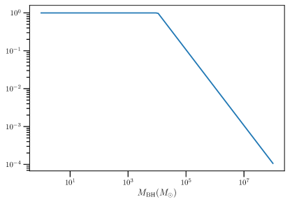
Figure 2: PBH accretion wind outflow duty cycle $\mathcal{D}$, for characteristic $v=10$ km/s and system radius $r_{\rm sys}=1$ pc.

4 Astrophysical Systems

We now apply our analysis to two examples of astrophysical systems, namely Milky Way gas clouds and dwarf galaxies. Although we limit our analysis to these systems, the methods outlined here can be readily extended to other gas clouds. Requiring the thermal balance of the gas cloud between standard cooling processes and heating from PBH, we constrain the PBH mass fraction $f_{\textrm{PBH}}$. A similar approach has been used to set limits on particle DM Bhoonah:2018wmw ; Farrar:2019qrv ; Wadekar:2019mpc . We find that for PBHs the different heating processes are particularly favorable to explore within the dwarf galaxy Leo T.

Natural heating sources (e.g. stellar radiation) are for simplicity neglected in this study, which results in a more conservative upper bound on PBH heating. Since our argument relies on maintaining thermal equilibrium, only gas systems that are expected to be stable on sufficiently long timescales $\tau_{\textrm{sys}}$ are used (see discussion in Ref. Farrar:2019qrv ). We thus require the timescale for which the gas system remains stable to be longer than the cooling timescale of the gas $\tau_{\textrm{therm}}$

$$\tau_{\textrm{sys}}\gg\tau_{\textrm{therm}}=\frac{3nkT}{2\dot{C}}~{},$$ (48)

where $k$ is the Boltzmann constant and $\dot{C}$ is the gas cooling rate per volume.

Furthermore, the disk formation timescale needs to be smaller than the system crossing timescale. This is directly analogous to the duty cycle considerations of Section 3.3.1 and is satisfied for our systems of interest. In the case of Leo T, this is not strictly necessary, since PBHs may orbit about the center of the dwarf galaxy. On the other hand, this could affect Milky Way cloud considerations, as PBHs do not spend all of their time inside them.

In principle a multitude of processes can participate in gas temperature exchange, and there exist detailed numerical analyses involving a full chemistry network Smith:2016hsc . We employ approximate results obtained in Ref. Wadekar:2019mpc for our gas systems of interest. The volumetric cooling rate (erg cm^-3 s^-1) of atomic hydrogen gas is given by

$$\dot{C}=n^{2}10^{[\textrm{Fe/H}]}\Lambda(T)~{},$$ (49)

where [Fe/H]$\equiv\log_{10}(n_{\rm Fe}/n_{\rm H})_{\rm gas}-\log_{10}(n_{\rm Fe}/n_{\rm H})_{\rm Sun}$ is the metallicity, and $\Lambda(T)\propto 10^{[{\rm Fe/H}]}$ is the cooling function which can be fitted numerically. Using the results from Ref. Smith:2016hsc library, Ref. Wadekar:2019mpc obtained $\Lambda(T)=2.51\times 10^{-28}T^{0.6}$ (erg cm³ s^-1), valid in the range $300~{}\text{K}<T<8000~{}\text{K}$.

The total heat deposited in the cloud by the PBH

$$H_{\rm tot}=N_{\textrm{PBH}}H(M)=f_{\textrm{PBH}}\dfrac{\rho_{\textrm{DM}}VH(M)}{M}$$ (50)

is required to be less than the total cooling rate $\dot{C}V$, yielding the condition on the PBH mass fraction

$$f_{\textrm{PBH}}<f_{\textrm{bound}}=\frac{M\dot{C}}{\rho_{\textrm{DM}}H(M)}~{}.$$ (51)

Here $H(M)$ is the average heat deposited by one PBH of mass $M$.

4.1 Gas systems with bulk relative velocity with respect to the DM

A gas system with a bulk relative velocity $\vec{v}_{b}$ with respect to the Galactic frame, and thus the PBH in the DM, can be treated as follows. Without loss of generality, consider the frame in which the bulk velocity is rotated to the z direction. Then the one dimensional Maxwellian velocity distributions are

$$\begin{split}\begin{cases}\dfrac{df_{v,x}}{dv}(v_{x})=\dfrac{df_{v,y}}{dv}(v_{y})=\dfrac{1}{\sqrt{2\pi}\sigma_{v}}e^{-\frac{v_{x}^{2}}{2\sigma_{v}^{2}}}\\ \\ \dfrac{df_{v,z}}{dv}(v_{z})=\dfrac{1}{\sqrt{2\pi}\sigma_{v}}e^{-\frac{(v_{z}-v_{b})^{2}}{2\sigma_{v}^{2}}}\end{cases}\end{split}$$ (52)

Imposing the constraint $v^{2}=\sqrt{v_{x}^{2}+v_{y}^{2}+v_{z}^{2}}$, the relative velocity distribution is given by the integral

$$\dfrac{df_{v}}{dv}(v)~{}= ~{}\frac{1}{(2\pi)^{\frac{3}{2}}\sigma_{v}^{3}}\int_{-\infty}^{\infty}dv_{x}\int_{-\infty}^{\infty}dv_{y}\int_{-\infty}^{\infty}dv_{z}\delta(v^{2}-v_{x}^{2}-v_{y}^{2}-v_{z}^{2})e^{-\frac{v_{x}^{2}+v_{y}^{2}+(v_{z}-v_{b})^{2}}{2\sigma_{v}^{2}}}$$ (53)

$$= ~{}\frac{e^{-\frac{v^{2}+v_{b}^{2}}{2\sigma^{2}}}}{(2\pi)^{\frac{3}{2}}\sigma_{v}^{3}}\int_{-v}^{v}dv_{x}\int_{-\sqrt{v^{2}-v_{x}^{2}}}^{\sqrt{v^{2}-v_{x}^{2}}}dv_{y}\frac{v}{\sqrt{v^{2}-v_{x}^{2}-v_{y}^{2}}}\left[e^{-\frac{v_{b}\sqrt{v^{2}-v_{x}^{2}-v_{y}^{2}}}{\sigma_{v}^{2}}}+e^{-\frac{v_{b}\sqrt{v^{2}-v_{x}^{2}-v_{y}^{2}}}{\sigma_{v}^{2}}}\right]~{}.$$

Switching to polar velocity coordinates and simplifying,

$$\begin{split}\dfrac{df_{v}}{dv}(v)~{}=&~{}\frac{2\pi v}{(2\pi)^{\frac{3}{2}}\sigma_{v}^{3}}e^{-\frac{v^{2}+v_{b}^{2}}{2\sigma_{v}^{2}}}\int_{0}^{v}dv_{r}\frac{v_{r}}{\sqrt{v^{2}-v_{r}^{2}}}\left[e^{-\frac{v_{b}\sqrt{v^{2}-v_{r}^{2}}}{\sigma_{v}^{2}}}+e^{\frac{v_{b}\sqrt{v^{2}-v_{r}^{2}}}{\sigma_{v}^{2}}}\right]\\ ~{}=&~{}\frac{v}{\sqrt{2\pi}\sigma v_{b}}\left[e^{-\frac{(v-v_{b})^{2}}{2\sigma^{2}}}-e^{-\frac{(v+v_{b})^{2}}{2\sigma^{2}}}\right]~{}.\end{split}$$ (54)

In the limit $v_{b}\rightarrow 0$, Eq. (54) reproduces the standard Maxwellian distribution Eq. (8).

4.2 Milky-Way gas clouds

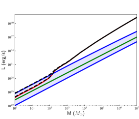
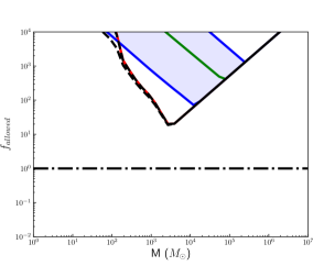
Figure 3: Left: Amount of heat absorbed by the Milky-Way gas cloud G33.4-8.0 from a single PBH of mass $M$. Right: Constraints from G33.4-8.0 on the DM fraction in PBHs. The reach of constraints is bounded by the positive slope solid black line indicating the incredulity limit. In both panels three heating components are shown: photon emission (red), dynamical friction (green), mass outflows (blue), as well as the total heat (black dashed). Both Model 1 and Model 2 of emission are shown, and the variation between them is shaded in blue. The observed line features are due to transitions between the eADAF, ADAF, LHAF, and thin disk regimes.

A variety of interstellar neutral hydrogen (HI) gas clouds exist in the inner Galaxy within a few hundred pc of the Galactic plane 2015ApJS..219…16P . In general, such Milky-Way clouds are not ideal candidates for studying PBHs due to the high relative rotational velocity, high velocity dispersion, and lower total DM mass (relative e.g. to dwarf galaxies) due to their smaller size. The last of these shortcomings limits the maximum mass considered for PBHs due to the incredulity limit of Eq. (7). Thus, even if a cloud had favorable properties otherwise, it would not be able to provide significant constraints in the intermediate PBH mass range.

To demonstrate our analysis, we consider as an example a particular Milky-May cloud, G33.4-8.0. To describe G33.4-8.0, we use parameters in Refs. 2015ApJS..219…16P ; 2015ApJS..216…29B ; 2004ApJ…602..162H ; 2002ApJ…580L..47L ; 2010ApJ…722..367F ; 2001ApJ…559..318R ; Wadekar:2019mpc . Namely, the atomic hydrogen gas density is taken to be $n=0.4~{}\pm 0.1\textrm{ cm}^{-3}$, the cloud radius $r\simeq 30\textrm{ pc}$, the bulk relative velocity $v_{\rm bulk}=220\textrm{ km/s}$, the temperature $T=400~{}\pm 90$ K, and the corresponding adiabatic sound speed $c_{s}=2.4\textrm{ km/s}$, and the cooling rate of $\simeq 2.1\times 10^{-27}\textrm{ erg}\textrm{ cm}^{-3}\textrm{ s}^{-1}$. The DM density of the cloud is $\rho=0.64\textrm{ GeV}/\textrm{cm}^{3}$, assuming Navarro-Frenk-White (NFW) profile Navarro:1995iw for the Galactic DM halo, with the DM velocity dispersion of $124.4\textrm{ km/s}$.

In Fig. 3, we display the heating from a single PBH for G33.4-8.0, including contributions due to photon emission, dynamical friction and mass outflows. To obtain the limits in Fig. 3, we numerically integrate Eq. (9). To treat the PBH emission and its uncertainty, we consider two distinct input parameter sets given in Table 1. The observed irregularities in the figure are due to transitions between the eADAF, ADAF, LHAF, and thin disk regimes.

We also display in Fig. 3 the combined resulting constraints from G33.4-8.0 gas heating, bound by the incredulity limit

$$f_{\textrm{bound}}>5.25\times 10^{-4}\left(\frac{M}{M_{\odot}}\right)\left(\frac{r_{\textrm{sys}}}{30\textrm{ pc}}\right)^{-3}\left(\frac{\rho_{\textrm{DM}}}{0.64\textrm{ GeV}\textrm{ cm}^{-3}}\right)^{-1}~{}.$$ (55)

The largest PBH mass that can be bounded by G33.4-8.0 with this method is $1.9\times 10^{3}M_{\odot}$. The weakness of Milky Way gas cloud bounds is due in large part to the high velocity dispersion as well as the co-rotation of the gas clouds in the Milky Way, which adversely affects accretion disk formation. In addition, the low metallicity of Leo T contributes to reduced cooling rates relative to G33.4-8.0 enhancing the effect of PBH heating.

	$\delta$	$\beta$	$\alpha$	$s$	$r_{\rm outer}$	$f_{k}$	$\mathcal{D}$
Model 1	0.3	10/11	0.1	0.5	$r_{B}$	0.1	1
Model 2	0.3	10/11	0.1	0.7	$100r_{s}$	0.2	1

Table 1: Input parameters for PBH emission.

4.3 Dwarf galaxies

Dwarf DM-rich galaxies provide a good setting to study DM-gas heating. In contrast to Milky-Way gas clouds, their lack of relative bulk velocity with respect to the DM as well as significant size that allows to weaken the incredulity limit makes them favorable systems for PBH heating.

We will focus on Leo T, a transition type of galaxy between a dwarf irregular and a spheroidal, which is a few hundred kpc away from the Milky Way. Leo T has been well studied and modeled theoretically and it has the desired properties, including low baryon velocity dispersion that is also favorable for PBH heating.

In the inner $r\lesssim 350\textrm{ pc}$ of Leo T, the gas is mostly composed of atomic hydrogen, but consists of highly ionized hydrogen outside this central region 2013ApJ…777..119F . To minimize the cooling rate, we avoid the efficiently cooled ionized region (see e.g. Ref. Smith:2016hsc ) and focus our analysis on the central region. The atomic hydrogen number density ranges from a maximum of $\sim 0.2\textrm{ cm}^{-3}$ at the center decreasing to $0.03\textrm{ cm}^{-3}$ at the boundary, at $r=350\textrm{ pc}$ 2013ApJ…777..119F . We estimate the density to be a constant $0.07\textrm{ cm}^{-3}$ (roughly the average density in the central region), and justify this by noting that both the heating processes and cooling rate scale approximately as $n^{2}$. This average density of gas produces the column density of $nr_{\textrm{sys}}=7.56\times 10^{19}\textrm{ cm}^{-2}$, in the right range for Leo T. Similarly, we assume a constant DM density of $1.75\textrm{ GeV}/\textrm{cm}^{3}$ which accounts for the total DM mass in Leo T of $10^{7}M_{\odot}$.

The hydrogen gas in the central region of Leo T is comprised both of a non-rotating warm component with velocity dispersion of $\sigma_{g}=6.9~{}\textrm{km}/\textrm{s}$ and temperature $T\simeq 6000$ K 2008MNRAS.384..535R ; 2013ApJ…777..119F as well as a subdominant cold component. For simplicity, we treat the entire hydrogen density as warm gas which results in a more conservative bound. From the adiabatic formula, the sound speed is estimated to be $c_{s}\simeq 9\textrm{ km/s}$ for a $6000$ K gas. The DM velocity dispersion is expected to be the same as the gas dispersion, so that $\sigma_{v}=\sigma_{g}$. Using the above input parameters as well as metallicity of $\textrm{[Fe/H]}\simeq-2$ 2008ApJ…685L..43K and assuming that gas metallicity is related to stellar metallicity in Eq. (49), the resulting Leo T’s cooling rate is taken to be $\dot{C}=2.28\times 10^{-30}\textrm{ erg}\textrm{ cm}^{-3}\textrm{ s}^{-1}$.

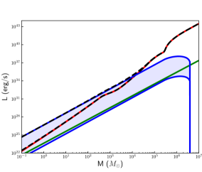
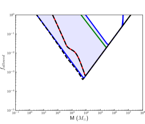
Figure 4: Left: The amount of heat absorbed by Leo T dwarf galaxy from a single PBH of mass $M$. Right: Constraints from Leo T on the DM fraction in PBHs. The reach of constraints is bounded by the positive slope solid black line indicating the incredulity limit. The variation in the constraint from Models 1 and 2 are shaded in blue. The black line shows the combined constraint from Model 2. For both panels three heating components are shown: photon emission (red), dynamical friction (green), mass outflows (blue), as well as the total heat (black). The observed line features are due to transitions between the eADAF, ADAF, LHAF, and thin disk regimes. Both Model 1 and Model 2 of emission are shown, and the difference is shaded in blue.

In Fig. 4, we display the heating from a single PBH for Leo T, including contributions due to photon emission, dynamical friction as well as mass outflows. As before, we numerically integrate Eq. (9) and consider PBH emission parameter variation as described in Tab. 1. We note that for the Leo T parameters, the condition for thin disks, $\dot{m}>0.07\alpha$, is satisfied only for very massive PBHs $M\gtrsim 10^{5}M_{\odot}$.

We also display in Fig. 4 the combined resulting Leo T gas heating constraints, bound by the incredulity limit

$$f_{\textrm{bound}}>1.21\times 10^{-7}\left(\frac{M}{M_{\odot}}\right)\left(\frac{r_{\textrm{sys}}}{350\textrm{ pc}}\right)^{-3}\left(\frac{\rho_{\textrm{DM}}}{1.75\textrm{ GeV}\textrm{ cm}^{-3}}\right)^{-1}~{}.$$ (56)

The largest PBH mass that can be bound by Leo T by this method is $8.26\times 10^{6}M_{\odot}$.

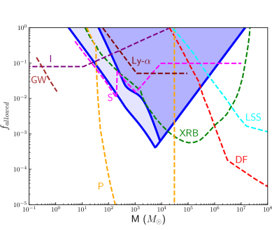
Figure 5: Constraints from Leo T dwarf galaxy on PBH gas heating are shown in blue. The light blue shaded band denotes variation due to PBH emission parameters. These constraints are bounded by the PBH incredulity limit (solid blue positive slope line). Other existing constraints (see Ref. (Carr:2020gox, )) are shown by dashed lines, including Icarus 2018PhRvD..97b3518O (I) caustic crossing in purple, Planck Ali-Haimoud:2016mbv ; Serpico:2020ehh (P) in yellow, X-ray binaries Inoue:2017csr (XRB) in green, dynamical friction of halo objects (DF) in red, Lyman-$\alpha$ 2019PhRvL.123g1102M (Ly-$\alpha$) in maroon, combined bounds from the survival of astrophysical systems in Eridanus II Brandt:2016aco , Segue 1 2017PhRvL.119d1102K , and disruption of wide binaries 2014ApJ…790..159M (S) shown in magenta, large scale structure Carr:2018rid (LSS) in cyan, and gravitational waves LIGOScientific:2019kan (GW) in brown.

5 Conclusions

PBHs in the stellar as well as intermediate $\sim 10-10^{3}~{}M_{\odot}$ mass-range have garnished significant interest and could potentially be associated with LIGO gravity wave events. As PBHs traverse the ISM, they would interact with and heat the surrounding gas. We have considered several generic heating mechanisms, including accretion photon emission, dynamical friction as well as mass outflows/winds. The balance of system heating and cooling allows for a general test of PBHs in a cosmology-independent way. As a demonstration, we have applied our analysis to Milky-Way gas clouds and dwarf galaxies. Considering constraints on gas heating for a given gas system, we have derived new bounds from Leo T dwarf galaxy on PBHs contributing to DM across a broad mass-range of $M_{\rm PBH}\sim\mathcal{O}(1)M_{\odot}-10^{7}M_{\odot}$. These limits do not depend on cosmology and establish a novel independent test of PBHs constituting part of the DM in the stellar and intermediate PBH mass range. Our analysis can be readily applied to other astrophysical systems of interest.

- (1) Y. B. Zel’dovich and I. D. Novikov, The Hypothesis of Cores Retarded during Expansion and the Hot Cosmological Model, Sov. Astron. 10 (1967) 602.
- (2) S. Hawking, Gravitationally collapsed objects of very low mass, Mon. Not. Roy. Astron. Soc. 152 (1971) 75.
- (3) B. J. Carr and S. W. Hawking, Black holes in the early Universe, Mon. Not. Roy. Astron. Soc. 168 (1974) 399.
- (4) M. Y. Khlopov and A. G. Polnarev, Primordial Black Holes as a Cosmological Test of Grand Unification, Phys. Lett. B 97 (1980) 383.
- (5) M. Khlopov, B. A. Malomed and I. B. Zeldovich, Gravitational instability of scalar fields and formation of primordial black holes, Mon. Not. Roy. Astron. Soc. 215 (1985) 575.
- (6) M. Kawasaki, N. Sugiyama and T. Yanagida, Primordial black hole formation in a double inflation model in supergravity, Phys. Rev. D 57 (1998) 6050 [hep-ph/9710259].
- (7) J. Garcia-Bellido, A. D. Linde and D. Wands, Density perturbations and black hole formation in hybrid inflation, Phys. Rev. D54 (1996) 6040 [astro-ph/9605094].
- (8) M. Yu. Khlopov, Primordial Black Holes, Res. Astron. Astrophys. 10 (2010) 495 [0801.0116].
- (9) P. H. Frampton, M. Kawasaki, F. Takahashi and T. T. Yanagida, Primordial Black Holes as All Dark Matter, JCAP 1004 (2010) 023 [1001.2308].
- (10) M. Kawasaki, A. Kusenko, Y. Tada and T. T. Yanagida, Primordial black holes as dark matter in supergravity inflation models, Phys. Rev. D94 (2016) 083523 [1606.07631].
- (11) B. Carr, F. Kuhnel and M. Sandstad, Primordial Black Holes as Dark Matter, Phys. Rev. D94 (2016) 083504 [1607.06077].
- (12) K. Inomata, M. Kawasaki, K. Mukaida, Y. Tada and T. T. Yanagida, Inflationary primordial black holes for the LIGO gravitational wave events and pulsar timing array experiments, Phys. Rev. D 95 (2017) 123510 [1611.06130].
- (13) S. Pi, Y.-l. Zhang, Q.-G. Huang and M. Sasaki, Scalaron from -gravity as a heavy field, JCAP 1805 (2018) 042 [1712.09896].
- (14) K. Inomata, M. Kawasaki, K. Mukaida, Y. Tada and T. T. Yanagida, Inflationary Primordial Black Holes as All Dark Matter, Phys. Rev. D 96 (2017) 043504 [1701.02544].
- (15) J. Garcia-Bellido, M. Peloso and C. Unal, Gravitational Wave signatures of inflationary models from Primordial Black Hole Dark Matter, JCAP 1709 (2017) 013 [1707.02441].
- (16) J. Georg and S. Watson, A Preferred Mass Range for Primordial Black Hole Formation and Black Holes as Dark Matter Revisited, JHEP 09 (2017) 138 [1703.04825].
- (17) K. Inomata, M. Kawasaki, K. Mukaida and T. T. Yanagida, Double inflation as a single origin of primordial black holes for all dark matter and LIGO observations, Phys. Rev. D 97 (2018) 043514 [1711.06129].
- (18) B. Kocsis, T. Suyama, T. Tanaka and S. Yokoyama, Hidden universality in the merger rate distribution in the primordial black hole scenario, Astrophys. J. 854 (2018) 41 [1709.09007].
- (19) K. Ando, K. Inomata, M. Kawasaki, K. Mukaida and T. T. Yanagida, Primordial black holes for the LIGO events in the axionlike curvaton model, Phys. Rev. D 97 (2018) 123512 [1711.08956].
- (20) E. Cotner and A. Kusenko, Primordial black holes from supersymmetry in the early universe, Phys. Rev. Lett. 119 (2017) 031103 [1612.02529].
- (21) E. Cotner and A. Kusenko, Primordial black holes from scalar field evolution in the early universe, Phys. Rev. D96 (2017) 103002 [1706.09003].
- (22) E. Cotner, A. Kusenko and V. Takhistov, Primordial Black Holes from Inflaton Fragmentation into Oscillons, Phys. Rev. D98 (2018) 083513 [1801.03321].
- (23) M. Sasaki, T. Suyama, T. Tanaka and S. Yokoyama, Primordial black holes—perspectives in gravitational wave astronomy, Class. Quant. Grav. 35 (2018) 063001 [1801.05235].
- (24) B. Carr and J. Silk, Primordial Black Holes as Generators of Cosmic Structures, Mon. Not. Roy. Astron. Soc. 478 (2018) 3756 [1801.00672].
- (25) U. Banik, F. C. van den Bosch, M. Tremmel, A. More, G. Despali, S. More et al., Constraining the mass density of free-floating black holes using razor-thin lensing arcs, Mon. Not. Roy. Astron. Soc. 483 (2019) 1558 [1811.00637].
- (26) F. Hoyle and R. A. Lyttleton, The effect of interstellar matter on climatic variation, Proceedings of the Cambridge Philosophical Society 35 (1939) 405.
- (27) E. Cotner, A. Kusenko, M. Sasaki and V. Takhistov, Analytic Description of Primordial Black Hole Formation from Scalar Field Fragmentation, JCAP 1910 (2019) 077 [1907.10613].
- (28) A. Kusenko, M. Sasaki, S. Sugiyama, M. Takada, V. Takhistov and E. Vitagliano, Exploring Primordial Black Holes from the Multiverse with Optical Telescopes, Phys. Rev. Lett. 125 (2020) 181304 [2001.09160].
- (29) M. M. Flores and A. Kusenko, Primordial Black Holes from Long-Range Scalar Forces and Scalar Radiative Cooling, Phys. Rev. Lett. 126 (2021) 041101 [2008.12456].
- (30) G. Domènech and M. Sasaki, Cosmology of strongly interacting fermions in the early universe, JCAP 06 (2021) 030 [2104.05271].
- (31) A. Katz, J. Kopp, S. Sibiryakov and W. Xue, Femtolensing by Dark Matter Revisited, JCAP 12 (2018) 005 [1807.11495].
- (32) N. Smyth, S. Profumo, S. English, T. Jeltema, K. McKinnon and P. Guhathakurta, Updated Constraints on Asteroid-Mass Primordial Black Holes as Dark Matter, Phys. Rev. D 101 (2020) 063005 [1910.01285].
- (33) P. Montero-Camacho, X. Fang, G. Vasquez, M. Silva and C. M. Hirata, Revisiting constraints on asteroid-mass primordial black holes as dark matter candidates, JCAP 1908 (2019) 031 [1906.05950].
- (34) S. Sugiyama, T. Kurita and M. Takada, On the wave optics effect on primordial black hole constraints from optical microlensing search, Mon. Not. Roy. Astron. Soc. 493 (2020) 3632 [1905.06066].
- (35) H. Niikura et al., Microlensing constraints on primordial black holes with Subaru/HSC Andromeda observations, Nat. Astron. 3 (2019) 524 [1701.02151].
- (36) R. Bean and J. Magueijo, Could supermassive black holes be quintessential primordial black holes?, Phys. Rev. D66 (2002) 063505 [astro-ph/0204486].
- (37) M. Kawasaki, A. Kusenko and T. T. Yanagida, Primordial seeds of supermassive black holes, Phys. Lett. B711 (2012) 1 [1202.3848].
- (38) S. Clesse and J. Garcia-Bellido, Massive Primordial Black Holes from Hybrid Inflation as Dark Matter and the seeds of Galaxies, Phys. Rev. D92 (2015) 023524 [1501.07565].
- (39) G. M. Fuller, A. Kusenko and V. Takhistov, Primordial Black Holes and -Process Nucleosynthesis, Phys. Rev. Lett. 119 (2017) 061101 [1704.01129].
- (40) V. Takhistov, Positrons from Primordial Black Hole Microquasars and Gamma-ray Bursts, Phys. Lett. B789 (2019) 538 [1710.09458].
- (41) V. Takhistov, Transmuted Gravity Wave Signals from Primordial Black Holes, Phys. Lett. B782 (2018) 77 [1707.05849].
- (42) V. Takhistov, G. M. Fuller and A. Kusenko, Test for the Origin of Solar Mass Black Holes, Phys. Rev. Lett. 126 (2021) 071101 [2008.12780].
- (43) T. Nakamura, M. Sasaki, T. Tanaka and K. S. Thorne, Gravitational waves from coalescing black hole MACHO binaries, Astrophys. J. Lett. 487 (1997) L139 [astro-ph/9708060].
- (44) S. Bird et al., Did LIGO detect dark matter?, Phys. Rev. Lett. 116 (2016) 201301 [1603.00464].
- (45) M. Raidal, V. Vaskonen and H. Veermäe, Gravitational Waves from Primordial Black Hole Mergers, JCAP 09 (2017) 037 [1707.01480].
- (46) Y. N. Eroshenko, Gravitational waves from primordial black holes collisions in binary systems, J. Phys. Conf. Ser. 1051 (2018) 012010 [1604.04932].
- (47) M. Sasaki, T. Suyama, T. Tanaka and S. Yokoyama, Primordial Black Hole Scenario for the Gravitational-Wave Event GW150914, Phys. Rev. Lett. 117 (2016) 061101 [1603.08338].
- (48) S. Clesse and J. García-Bellido, Detecting the gravitational wave background from primordial black hole dark matter, Phys. Dark Univ. 18 (2017) 105 [1610.08479].
- (49) Virgo, LIGO Scientific collaboration, B. P. Abbott et al., Observation of Gravitational Waves from a Binary Black Hole Merger, Phys. Rev. Lett. 116 (2016) 061102 [1602.03837].
- (50) Virgo, LIGO Scientific collaboration, B. P. Abbott et al., GW151226: Observation of Gravitational Waves from a 22-Solar-Mass Binary Black Hole Coalescence, Phys. Rev. Lett. 116 (2016) 241103 [1606.04855].
- (51) VIRGO, LIGO Scientific collaboration, B. P. Abbott et al., GW170104: Observation of a 50-Solar-Mass Binary Black Hole Coalescence at Redshift 0.2, Phys. Rev. Lett. 118 (2017) 221101 [1706.01812].
- (52) LIGO Scientific, Virgo collaboration, R. Abbott et al., GW190521: A Binary Black Hole Merger with a Total Mass of 150 M, Phys. Rev. Lett. 125 (2020) 101102 [2009.01075].
- (53) B. Carr, K. Kohri, Y. Sendouda and J. Yokoyama, Constraints on Primordial Black Holes, 2002.12778.
- (54) P. Lu, V. Takhistov, G. B. Gelmini, K. Hayashi, Y. Inoue and A. Kusenko, Constraining Primordial Black Holes with Dwarf Galaxy Heating, Astrophys. J. Lett. 908 (2021) L23 [2007.02213].
- (55) B. J. Carr and M. Sakellariadou, Dynamical Constraints on Dark Matter in Compact Objects, Astrophys. J. 516 (1999) 195.
- (56) C. G. Lacey and J. P. Ostriker, Massive black holes in galactic halos ?, Astrophys. J. 299 (1985) 633.
- (57) T. Totani, Size Evolution of Early-Type Galaxies and Massive Compact Objects as Dark Matter, PASJ 62 (2010) L1 [0908.3295].
- (58) D. Gaggero, G. Bertone, F. Calore, R. M. T. Connors, M. Lovell, S. Markoff et al., Searching for Primordial Black Holes in the radio and X-ray sky, Phys. Rev. Lett. 118 (2017) 241101 [1612.00457].
- (59) Y. Inoue and A. Kusenko, New X-ray bound on density of primordial black holes, JCAP 1710 (2017) 034 [1705.00791].
- (60) A. Hektor, G. Hütsi and M. Raidal, Constraints on primordial black hole dark matter from Galactic center X-ray observations, Astron. Astrophys. 618 (2018) A139 [1805.06513].
- (61) A. Bhoonah, J. Bramante, F. Elahi and S. Schon, Calorimetric Dark Matter Detection With Galactic Center Gas Clouds, Phys. Rev. Lett. 121 (2018) 131101 [1806.06857].
- (62) G. R. Farrar, F. J. Lockman, N. McClure-Griffiths and D. Wadekar, Comment on the paper ”Calorimetric Dark Matter Detection with Galactic Center Gas Clouds”, Phys. Rev. Lett. 124 (2020) 029001 [1903.12191].
- (63) D. Wadekar and G. R. Farrar, Gas-rich dwarf galaxies as a new probe of dark matter interactions with ordinary matter, Phys. Rev. D 103 (2021) 123028 [1903.12190].
- (64) M. Ricotti, J. P. Ostriker and K. J. Mack, Effect of Primordial Black Holes on the Cosmic Microwave Background and Cosmological Parameter Estimates, Astrophys. J. 680 (2008) 829 [0709.0524].
- (65) A. Hektor, G. Hütsi, L. Marzola, M. Raidal, V. Vaskonen and H. Veermäe, Constraining Primordial Black Holes with the EDGES 21-cm Absorption Signal, Phys. Rev. D 98 (2018) 023503 [1803.09697].
- (66) O. Mena, S. Palomares-Ruiz, P. Villanueva-Domingo and S. J. Witte, Constraining the primordial black hole abundance with 21-cm cosmology, Phys. Rev. D 100 (2019) 043540 [1906.07735].
- (67) E. Agol and M. Kamionkowski, X-rays from isolated black holes in the Milky Way, Mon. Not. Roy. Astron. Soc. 334 (2002) 553 [astro-ph/0109539].
- (68) H. Bondi and F. Hoyle, On the mechanism of accretion by stars, Mon. Not. Roy. Astron. Soc. 104 (1944) 273.
- (69) H. Bondi, On spherically symmetrical accretion, Mon. Not. Roy. Astron. Soc. 112 (1952) 195.
- (70) M. Guo, K. Inayoshi, T. Michiyama and L. C. Ho, Hunting for wandering massive black holes, Astrophys. J. 901 (2020) 39 [2006.08203].
- (71) S. Kato, J. Fukue and S. Mineshige, Black-Hole Accretion Disks — Towards a New Paradigm —. 2008.
- (72) N. Shakura and R. Sunyaev, Black holes in binary systems. Observational appearance, Astron. Astrophys. 24 (1973) 337.
- (73) S. L. Shapiro and A. P. Lightman, Black holes in X-ray binaries: marginal existence and rotation reversals of accretion disks., Astrophys. J. 204 (1976) 555.
- (74) R. Narayan and I.-s. Yi, Advection dominated accretion: A Selfsimilar solution, Astrophys. J. Lett. 428 (1994) L13 [astro-ph/9403052].
- (75) F. Yuan and R. Narayan, Hot accretion flows around black holes, Ann. Rev. Astron. Astrophys. 52 (2014) 529 [1401.0586].
- (76) K. Hayashi and M. Chiba, Probing non-spherical dark halos in the Galactic dwarf galaxies, Astrophys. J. 755 (2012) 145 [1206.3888].
- (77) H. Kim, A constraint on light primordial black holes from the interstellar medium temperature, Mon. Not. Roy. Astron. Soc. 504 (2021) 5475 [2007.07739].
- (78) R. Laha, P. Lu and V. Takhistov, Gas heating from spinning and non-spinning evaporating primordial black holes, Phys. Lett. B 820 (2021) 136459 [2009.11837].
- (79) J.-M. Wang, E. Szuszkiewicz, F.-J. Lu and Y.-Y. Zhou, Emergent Spectra from Slim Accretion Disks in Active Galactic Nuclei, Astrophys. J. 522 (1999) 839.
- (80) H. A. Bethe and E. E. Salpeter, Quantum Mechanics of One- and Two-Electron Systems, pp. 88–436. Springer Berlin Heidelberg, Berlin, Heidelberg, 1957.
- (81) I. M. Band, M. B. Trzhaskovskaia, D. A. Verner and D. G. Iakovlev, K-shell photoionization cross sections - Calculations and simple fitting formulae, Astron. Astrophys. 237 (1990) 267.
- (82) K. Olive, Review of particle physics, Chinese Physics C 38 (2014) 090001.
- (83) J. M. Shull and M. E. van Steenberg, X-ray secondary heating and ionization in quasar emission-line clouds, Astrophys. J. 298 (1985) 268.
- (84) M. Ricotti, N. Y. Gnedin and J. Shull, The fate of the first galaxies. I. self-consistent cosmological simulations with radiative transfer, Astrophys. J. 575 (2002) 33 [astro-ph/0110431].
- (85) S. Furlanetto and S. J. Stoever, Secondary ionization and heating by fast electrons, Mon. Not. Roy. Astron. Soc. 404 (2010) 1869 [0910.4410].
- (86) J. Pringle, Accretion discs in astrophysics, Ann. Rev. Astron. Astrophys. 19 (1981) 137.
- (87) F. Yuan, E. Quataert and R. Narayan, Nonthermal Electrons in Radiatively Inefficient Accretion Flow Models of Sagittarius A*, Astrophys. J. 598 (2003) 301 [astro-ph/0304125].
- (88) R. Mahadevan, Scaling laws for advection dominated flows: Applications to low luminosity galactic nuclei, Astrophys. J. 477 (1997) 585 [astro-ph/9609107].
- (89) R. Narayan and I. Yi, Advection-dominated Accretion: Underfed Black Holes and Neutron Stars, Astrophys. J. 452 (1995) 710 [astro-ph/9411059].
- (90) J. Binney and S. Tremaine, Galactic Dynamics: Second Edition. 2008.
- (91) E. C. Ostriker, Dynamical Friction in a Gaseous Medium, Astrophys. J. 513 (1999) 252 [astro-ph/9810324].
- (92) R. D. Blandford and M. C. Begelman, On the fate of gas accreting at a low rate onto a black hole, Mon. Not. Roy. Astron. Soc. 303 (1999) L1 [astro-ph/9809083].
- (93) T. Totani, A RIAF Interpretation for the Past Higher Activity of the Galactic Center Black Hole and the 511 keV Annihilation Emission, Publ. Astron. Soc. Jpn. 58 (2006) 965 [astro-ph/0607414].
- (94) F. Yuan, D. Bu and M. Wu, Numerical Simulation of Hot Accretion Flows. II. Nature, Origin, and Properties of Outflows and their Possible Observational Applications, Astrophys. J. 761 (2012) 130 [1206.4173].
- (95) F.-G. Xie and F. Yuan, The Radiative Efficiency of Hot Accretion Flows, Mon. Not. Roy. Astron. Soc. 427 (2012) 1580 [1207.3113].
- (96) B. Pang, U.-L. Pen, C. D. Matzner, S. R. Green and M. Liebendörfer, Numerical parameter survey of non-radiative black hole accretion: flow structure and variability of the rotation measure, Mon. Not. Roy. Astron. Soc. 415 (2011) 1228 [1011.5498].
- (97) J. Li, J. Ostriker and R. Sunyaev, Rotating Accretion Flows: From Infinity to the Black Hole, Astrophys. J. 767 (2013) 105 [1206.4059].
- (98) F. Yuan, D. Bu and M. Wu, Outflow from Hot Accretion Flows, in Feeding Compact Objects: Accretion on All Scales (C. M. Zhang, T. Belloni, M. Méndez and S. N. Zhang, eds.), vol. 290 of IAU Symposium, pp. 86–89, Feb., 2013, 1210.6093, DOI.
- (99) J. J. Bailey, I. B. Abdurakhmanov, A. S. Kadyrov, I. Bray and A. M. Mukhamedzhanov, Proton-beam stopping in hydrogen, Phys. Rev. A 99 (2019) 042701.
- (100) F. H. Panther, Positron Transport and Annihilation in the Galactic Bulge, Galaxies 6 (2018) 39 [1801.09365].
- (101) K. Ioka, T. Matsumoto, Y. Teraki, K. Kashiyama and K. Murase, GW 150914-like black holes as Galactic high-energy sources, Mon. Not. Roy. Astron. Soc. 470 (2017) 3332 [1612.03913].
- (102) B. D. Smith et al., Grackle: a Chemistry and Cooling Library for Astrophysics, Mon. Not. Roy. Astron. Soc. 466 (2017) 2217 [1610.09591].
- (103) Y. Pidopryhora, F. J. Lockman, J. M. Dickey and M. P. Rupen, High-resolution Images of Diffuse Neutral Clouds in the Milky Way. I. Observations, Imaging, and Basic Cloud Properties, Astrophys. J. Supp. 219 (2015) 16 [1506.03873].
- (104) J. Bovy, galpy: A python Library for Galactic Dynamics, Astrophys. J. Supp. 216 (2015) 29 [1412.3451].
- (105) M. Hoeft, J. P. Mücket and S. Gottlöber, Velocity Dispersion Profiles in Dark Matter Halos, Astrophys. J. 602 (2004) 162 [astro-ph/0311083].
- (106) F. J. Lockman, Discovery of a Population of H I Clouds in the Galactic Halo, Astrophys. J. Lett. 580 (2002) L47 [astro-ph/0210424].
- (107) H. A. Ford, F. J. Lockman and N. M. McClure-Griffiths, Milky Way Disk-Halo Transition in H I: Properties of the Cloud Population, Astrophys. J. 722 (2010) 367 [1008.2760].
- (108) P. Richter, K. R. Sembach, B. P. Wakker, B. D. Savage, T. M. Tripp, E. M. Murphy et al., The Diversity of High- and Intermediate-Velocity Clouds: Complex C versus IV Arch, Astrophys. J. 559 (2001) 318 [astro-ph/0105466].
- (109) J. F. Navarro, C. S. Frenk and S. D. M. White, The Structure of cold dark matter halos, Astrophys. J. 462 (1996) 563 [astro-ph/9508025].
- (110) Y. Faerman, A. Sternberg and C. F. McKee, Ultra-compact High Velocity Clouds as Minihalos and Dwarf Galaxies, Astrophys. J. 777 (2013) 119 [1309.0815].
- (111) E. V. Ryan-Weber, A. Begum, T. Oosterloo, S. Pal, M. J. Irwin, V. Belokurov et al., The Local Group dwarf Leo T: HI on the brink of star formation, Mon. Not. Roy. Astron. Soc. 384 (2008) 535 [0711.2979].
- (112) E. N. Kirby, J. D. Simon, M. Geha, P. Guhathakurta and A. Frebel, Uncovering Extremely Metal-Poor Stars in the Milky Way’s Ultrafaint Dwarf Spheroidal Satellite Galaxies, Astrophys. J. Lett. 685 (2008) L43 [0807.1925].
- (113) M. Oguri, J. M. Diego, N. Kaiser, P. L. Kelly and T. Broadhurst, Understanding caustic crossings in giant arcs: Characteristic scales, event rates, and constraints on compact dark matter, Phys. Rev. D 97 (2018) 023518 [1710.00148].
- (114) Y. Ali-Haïmoud and M. Kamionkowski, Cosmic microwave background limits on accreting primordial black holes, Phys. Rev. D95 (2017) 043534 [1612.05644].
- (115) P. D. Serpico, V. Poulin, D. Inman and K. Kohri, Cosmic microwave background bounds on primordial black holes including dark matter halo accretion, Phys. Rev. Res. 2 (2020) 023204 [2002.10771].
- (116) R. Murgia, G. Scelfo, M. Viel and A. Raccanelli, Lyman-alpha Forest Constraints on Primordial Black Holes as Dark Matter, Phys. Rev. Lett. 123 (2019) 071102 [1903.10509].
- (117) T. D. Brandt, Constraints on MACHO Dark Matter from Compact Stellar Systems in Ultra-Faint Dwarf Galaxies, Astrophys. J. Lett. 824 (2016) L31 [1605.03665].
- (118) S. M. Koushiappas and A. Loeb, Dynamics of Dwarf Galaxies Disfavor Stellar-Mass Black Holes as Dark Matter, Phys. Rev. Lett. 119 (2017) 041102 [1704.01668].
- (119) M. A. Monroy-Rodríguez and C. Allen, The End of the MACHO Era, Revisited: New Limits on MACHO Masses from Halo Wide Binaries, Astrophys. J. 790 (2014) 159 [1406.5169].
- (120) LIGO Scientific, Virgo collaboration, B. P. Abbott et al., Search for Subsolar Mass Ultracompact Binaries in Advanced LIGO’s Second Observing Run, Phys. Rev. Lett. 123 (2019) 161102 [1904.08976].