Quantum radiation of a collapsing shell in three-dimensional AdS spacetime revisited

Abstract

In three-dimensional AdS space, we consider the gravitational collapse of dust shell and then investigate the quantum radiation from the collapsing shell by employing the functional Schrödinger formalism. In the formation of the BTZ black hole, the interior geometry of the shell can be chosen as either the massless black hole or the global AdS space. In the incipient black hole limit, we obtain the wave function exactly from the time-dependent Schrödinger equation for a massless scalar field. Then, we show that the occupation number of excited states can be written by analytic expressions, and the radiation temperature is in agreement with the Hawking temperature, irrespective of the specific choice of the interior geometries.

I introduction

Since the discovery of Hawking radiation Hawking:1974sw , quantum black holes have been one of the most intriguing physical objects in quantum theory of gravity. In the semiclassical approximations, the total number of particles emitted from black holes turned out to be the Planckian distribution of thermal radiation Hawking:1974sw ; Hartle:1976tp ; Gibbons:1977mu ; Akhmedov:2015xwa .

On the other hand, there has been much attention to the collapse of the dust shell for the Schwarzschild black hole Boulware:1975fe ; Gerlach:1976ji ; 10.1143/PTP.81.826 ; Alberghi:1998xe ; Alberghi:2001cm and lower-dimensional black holes Mann:1992my ; Ross:1992ba ; Peleg:1994wx ; Crisostomo:2003xz ; Mann:2006yu ; Hyun:2006xt . In particular, the functional Schrödinger formalism was employed to investigate quantum radiation from the collapsing shell for the Schwarzschild metric Vachaspati:2006ki ; Vachaspati:2007hr ; Greenwood:2008zg ; Greenwood:2010sx ; Kolopanis:2013sty ; Saini:2015dea ; Saini:2016rrt . In fact, the advantage of the functional Schrödinger equation would be that wave functionals living on a space of field configurations explicitly depend on time Kiefer:1991xy . This functional Schrödinger formalism was also applied to the formation of various dynamical geometries such as the Reissner-Nordström black hole Greenwood:2009pd ; Das:2019iru , the black string in anti-de Sitter(AdS) space Greenwood:2009gp , the three-dimensional AdS black hole Saini:2017mur , and the regular black hole Um:2019qgc . In the formation of the black holes, the spectrum of quantum radiation is approximately thermal as the shell approaches its own horizon, and the temperature of the radiation is in agreement with the Hawking temperature of the corresponding black holes. In asymptotically flat black holes formed by collapsing shells, spacetime for the interior region of the shell was naturally prescribed by Minkowski spacetime because the interior region is assumed to be empty Vachaspati:2006ki ; Vachaspati:2007hr ; Greenwood:2008zg ; Greenwood:2009pd ; Greenwood:2010sx ; Kolopanis:2013sty ; Saini:2015dea ; Saini:2016rrt ; Das:2019iru ; Um:2019qgc .

In the asymptotically non-flat spacetime such as the nonrotating Bañados-Teitelboim-Zanelli (BTZ) black hole Banados:1992wn described by the line element

$$ds^{2}=-f(r)dt^{2}+\frac{1}{f(r)}dr^{2}+r^{2}d\phi^{2},$$ (1)

where $f(r)=-M+r^{2}/\ell^{2}$ with $M$ and $\ell$ being the mass parameter and the radius of curvature, respectively, the BTZ black hole is defined for $M>0$ and the massless black hole is for $M=0$. In addition, the global AdS space of a thermal soliton emerges as a bound state for $M=-1$ which has a lower energy than that of the massless black hole. In the formation of the BTZ black hole, the interior region of the shell could be chosen as the global AdS space ($M=-1$) Peleg:1994wx ; Crisostomo:2003xz or the massless black hole geometry ($M=0$) Saini:2017mur . For $M=0$, the radiation temperature was shown to be close to the Hawking temperature by explicit numerical analysis Saini:2017mur .

In this paper, we will revisit the quantum radiation by solving the functional Schrödinger equation analytically in the formation of the BTZ black hole. For this purpose, the exterior and interior regions of the dust shell will be described by the AdS geometry (1) characterized by different exterior and interior mass parameters of $M_{\rm out}$ and $M_{\rm in}$. The mass parameters are chosen as $M_{\rm out}>0$ and $M_{\rm in}=0,-1$. Namely, the vacuum state for the interior region is described by the massless black hole or the global AdS space. Importantly, in the incipient limit of $R\to R_{H}$ where $R$ is a shell radius, the occupation number will be expressed by explicit Bessel functions and it turns out to be independent of $M_{\rm in}$. After all, the radiation temperature is found to be close to the Hawking temperature.

The organization of this paper is as follows. In Sec. II, we will find a mass relation from the junction condition on the dust shell for arbitrary mass parameters of $M_{\rm out}$ and $M_{\rm in}$. Then, the functional Schrödinger equation from the action for a massless scalar field will be derived for the formation of the BTZ black hole. In Sec. III, the wave functions from the functional Schrödinger equations will be obtained analytically and the corresponding spectra of quantum radiation will be investigated. Finally, conclusion and discussion will be given in Sec. IV.

II Schrödinger equations for collapsing dust shell

II.1 Classical collapse of the shell

In this section, we provide a general formalism for the classical collapse of the shell in AdS space. Let us start with spacetime divided by an infinitely thin shell with a radius $R$ in three-dimensional AdS space. For the exterior and interior coordinates denoted by $\left(t,r,\phi\right)$ and $\left(T,r,\phi\right)$, the radius would be given as $R(t)$ which is a decreasing function of the time $t$.

For the exterior region of the shell, the spacetime is given by the line element

$$ds_{\rm(out)}^{2}=-f_{\rm out}(r)dt^{2}+\frac{1}{f_{\rm out}(r)}dr^{2}+r^{2}d\phi^{2}~{}~{}(r>R(t)),$$ (2)

where $f_{\rm out}(r)=-M_{\rm out}+r^{2}/\ell^{2}$. For the interior region of the shell, the line element is also described by

$$ds_{\rm(in)}^{2}=-f_{\rm in}(r)dT^{2}+\frac{1}{f_{\rm in}(r)}dr^{2}+r^{2}d\phi^{2}~{}~{}(r<R(t)),$$ (3)

where $f_{\rm in}(r)=-M_{\rm in}+r^{2}/\ell^{2}$. Thus, the line element at the shell is assumed to be

$$ds_{\rm(shell)}^{2}=-d\tau^{2}+R^{2}(t)d\phi^{2}~{}~{}(r=R(t))$$ (4)

with $\tau$ being the proper time of the collapsing shell. Since the line element should be continuous at the shell, Eqs. (2) and (3) are coincident with Eq. (4) at $r=R(t)$, which gives the relations between the time coordinates $t$ and $T$ as

$$\lambda(t)=\frac{dT}{dt}\bigg{|}_{r=R(t)}=\sqrt{\frac{f_{\rm out}(R)}{f_{\rm in}(R)}-\frac{1}{f_{\rm in}(R)}\left\{\frac{1}{f_{\rm out}(R)}-\frac{1}{f_{\rm in}(R)}\right\}\left(\frac{dR}{dt}\right)^{2}},$$ (5)

where we did not fix $f_{\rm out}(R)$ and $f_{\rm in}(R)$ for our general argument.

Next, we consider a combined metric tensor defined as $g_{\mu\nu}=\Theta(r-R(t))g^{\rm(out)}_{\mu\nu}+\Theta(-r+R(t))g^{\rm(in)}_{\mu\nu}$ where $\Theta(x)=1(x>0)$ and $\Theta(x)=0(x<0)$. Employing the first junction condition that the combined metric tensor is continuous on the shell, one can derive the projection of the Einstein equation onto the shell as Israel:1966rt

$$-\left[K_{\mu\nu}\right]+h_{\mu\nu}\left[K\right]=8\pi S_{\mu\nu},$$ (6)

where $K_{\mu\nu}=h_{\mu}^{\gamma}\nabla_{\gamma}n_{\nu}$, $K=g_{\mu}^{\gamma}K_{\gamma\nu}$, and $S_{\mu\nu}=h_{\mu}^{\gamma}T_{\gamma\nu}$ are the projections of the extrinsic curvature and the energy-momentum tensor of the shell, respectively. $[...]$ denotes $[A]=\lim_{r\to R+}A(r)-\lim_{r\to R-}A(r)$. And $h_{\mu\nu}=(g_{\mu\nu}-n_{\mu}n_{\nu})\big{|}_{r=R(t)}$ is a projection operator onto the shell with a normal vector of the shell $n_{\mu}$, where $h_{\mu\nu}$ automatically satisfies $h_{\mu}^{\gamma}h_{\gamma\nu}=h_{\mu\nu}$. We consider the dust shell and so its energy-momentum tensor is given as $S^{\mu\nu}=\sigma u^{\mu}u^{\nu}$, where $\sigma$ is the surface energy density of the shell and $u^{\mu}$ is the three-velocity at the shell. Taking the inner product to Eq. (6) with $u^{\mu}$ and $u^{\nu}$, one can finally get the so-called mass relation,

$$\sqrt{\dot{R}^{2}+f_{\rm out}(R)}-\sqrt{\dot{R}^{2}+f_{\rm in}(R)}=-8\pi\sigma R,$$ (7)

where $\dot{R}=dR/d\tau$. Note that Eq. (7) certainly shows that $\sigma>0$ for $M_{\rm out}>M_{\rm in}$ while $\sigma<0$ for $M_{\rm out}<M_{\rm in}$.

Plugging $f_{\rm out}(r)$ and $f_{\rm in}(r)$ in Eqs. (2) and (3) into Eq. (7), one can find

$$\dot{R}^{2}=\frac{1}{2}\left(M_{\rm out}+M_{\rm in}\right)+\left(\frac{f_{\rm out}(R)-f_{\rm in}(R)}{16\pi\sigma R}\right)^{2}+\left(\left(4\pi\sigma\right)^{2}-\frac{1}{\ell^{2}}\right)R^{2},$$ (8)

where we supposed that $(4\pi\sigma)^{2}>\ell^{-2}$ to make the shell collapse continuously even for an arbitrary large $R$. Using the relation of $\left(dR/dt\right)^{2}=\left(dt/d\tau\right)^{-2}\dot{R}^{2}$ for the collapsing shell, we get

$$\frac{dR}{dt}=-\frac{f_{\rm out}(R)\dot{R}}{\sqrt{f_{\rm out}(R)+\dot{R}^{2}}}.$$ (9)

II.2 The functional Schrödinger equation

To study the quantum radiation from the collapsing shell, we consider a minimally coupled scalar field $\Phi$. On the spacetime background described by Eqs. (2), (3), and (4), we consider the total action which consists of the sum of the exterior and interior actions as

$$S_{\rm(tot)}=S_{\rm(out)}+S_{\rm(in)},$$ (10)

$$S_{\rm(out)}=\pi\int dt\int_{R(t)}^{\infty}\!\!\!\!dr~{}\left(\frac{1}{f_{\rm out}(r)}\left(\partial_{t}\Phi\right)^{2}-f_{\rm out}(r)\left(\partial_{r}\Phi\right)^{2}\right),$$ (11)

$$S_{\rm(in)}=\pi\int dT\int^{R(t)}_{0}\!\!\!\!\!\!dr~{}\left(\frac{1}{f_{\rm in}(r)}\left(\partial_{T}\Phi\right)^{2}-f_{\rm in}(r)\left(\partial_{r}\Phi\right)^{2}\right).$$ (12)

For convenience, let us rewrite the interior action by using Eq. (5) as

$$S_{\rm(in)}=\pi\int dt\int^{R(t)}_{0}\!\!\!\!\!\!dr~{}\left(\frac{1}{\lambda(t)f_{\rm in}(r)}\left(\partial_{t}\Phi\right)^{2}-\lambda(t)f_{\rm in}(r)\left(\partial_{r}\Phi\right)^{2}\right).$$ (13)

From Eq. (10), the functional Schrödinger equation will be derived in the limit of $\lambda(t)\ll 1$, which will be shown to be of relevance to the incipient limit of the BTZ black hole of $R\to R_{H}$.

In order to study the formation of the BTZ black hole, we consider the configuration of $M_{\rm out}>0$ and $M_{\rm in}=0,-1$. In particular, for $M=-1$, nonsingular vortex solutions in AdS₃ background were numerically found Edery:2020kof . However, we will consider the global AdS space as a thermal soliton without any classical fields. As the radius of the shell approaches its horizon, $i.e.$, $R(t)\to R_{H}=\sqrt{M_{\rm out}}\ell$ called the incipient limit, Eq. (8) reduces to a finite value as $\dot{R}^{2}\approx\left.\left(f_{\rm in}(R)/(8\mu)-2\mu\right)^{2}\right|_{R=R_{H}}$, where $\mu$ is the constant of motion defined by $\mu=2\pi R\sigma$ Saini:2017mur . Thus, Eq. (9) in this limit also reduces to a simpler form as

$$\frac{dR}{dt}\approx-f_{\rm out}(R),$$ (14)

which yields the radius function as

$$R(t)=\begin{cases}R_{0}&(t<0),\\ R_{H}+\left(R_{0}-R_{H}\right)e^{-f_{\rm out}^{\prime}(R_{H})t}&(0\leq t\leq t_{f}),\\ R_{f}&(t>t_{f})~{},\end{cases}$$ (15)

where $t=0$ and $R_{0}$ are the initial time and radius, respectively. For a nice mathematical manipulation of infinite time, we artificially take the collapse to stop at some time $t=t_{f}$ with the radius $R_{f}$ defined as $R(t_{f})=R_{H}+(R_{0}-R_{H})e^{-f^{\prime}_{\rm out}(R_{H})t_{f}}$, where Eq. (15) is continuous at $t=t_{f}$, $i.e.$, $R_{f}=R(t_{f})$. Then we take the limit of $t_{f}\to\infty$ to investigate the eternal collapse case which implies that the shell collapses to form the black hole ($i.e.$, $R(t)\to R_{H}$), in other words, $R_{f}\to R_{H}$ in Eq. (15). Note that, if one considered up to the order of $(R-R_{H})^{2}$ in Eq. (7), $M_{\rm in}$ would appear in $(dR/dt)$ in such a way that $(dR/dt)\approx-f_{\rm out}(R)+f_{\rm out}^{2}(R)/(2\dot{R}^{2})$. However, as long as we are concerned with the lowest order of $(R-R_{H})$, $i.e.$, in the incipient limit, $(dR/dt)$ turns out to be independent of $M_{\rm in}$. Therefore, in the formation of the BTZ black hole, the choice of the interior region is not crucial as long as $M_{\rm out}>M_{\rm in}$.

From Eq. (9), Eq. (5) can be cast in the incipient limit as

$$\lambda(t)\approx\frac{16\mu^{2}+f_{\rm in}(R_{H})}{\left(16\mu^{2}-f_{\rm in}(R_{H})\right)f_{\rm in}(R_{H})}f_{\rm out}(R(t))$$ (16)

so that $\lambda(t)$ can be made very small because $f_{\rm out}\to 0$ near the horizon. For $\lambda(t)\ll 1$, the kinetic term in the exterior action (11) and the potential term in the interior action (13) can be ignored, and thus, the total action (10) is simplified as

$$S_{\rm(tot)}=\pi\int dt\left(\frac{1}{\lambda(t)}\int_{0}^{R(t)}\!\!\!\!\!\!dr~{}\frac{1}{f_{\rm in}(r)}\left(\partial_{t}\Phi\right)^{2}-\int_{R(t)}^{\infty}\!\!\!\!dr~{}f_{\rm out}(r)\left(\partial_{r}\Phi\right)^{2}\right).$$ (17)

After decomposition of $\Phi$ in terms of $\Phi=\sum_{k}a_{k}(t)d_{k}(r)$ and the simultaneous diagonalization of the following Hermitian operators goldstein:mechanics ; Vachaspati:2006ki , $A_{k,k^{\prime}}=2\pi\int_{0}^{R(t)}dr~{}d_{k}(r)d_{k^{\prime}}(r)/f_{\rm in}(r)$ and $B_{k,k^{\prime}}=2\pi\int_{R(t)}^{\infty}dr~{}f_{\rm out}(r)(dd_{k}(r)/dr)(dd_{k^{\prime}}(r)/dr)$, we obtain the total action (17) as

$$S_{\rm(tot)} = \int dtL_{\Phi}$$ (18)

$$= \sum_{k}\int dt\left(\frac{\alpha_{k}}{2\lambda(t)}\left(\frac{db_{k}(t)}{dt}\right)^{2}-\frac{1}{2}\beta_{k}b_{k}^{2}(t)\right),$$

where $\alpha_{k}$ and $\beta_{k}$ are eigenvalues of $A_{k,k^{\prime}}$ and $B_{k,k^{\prime}}$ for a set of eigenvectors $\{b_{k}\}$, respectively. For a mode amplitude $b_{k}(t)$, the conjugate momentum is defined as $\Pi_{k}=\partial L_{\Phi}/\partial\left(db_{k}(t)/dt\right)$ $=\alpha_{k}\lambda^{-1}(t)\left(db_{k}(t)/dt\right)$. Then, from the Legendre transformation of Eq. (18), the Hamiltonian can easily be obtained as $H_{\Phi}=\sum_{k}\left\{\lambda(t)/\left(2\alpha_{k}\right)\Pi_{k}^{2}+(1/2)\beta_{k}b_{k}^{2}\right\}$. Imposing the quantization rule $\left[b_{k}(t),\Pi_{k^{\prime}}\right]=i\delta_{k,k^{\prime}}$ where $\Pi_{k}\to-i\partial/\partial b_{k}$, we get the Hamiltonian for quantum radiation as

$$H_{\Phi}=\sum_{k}H_{\Phi,k}=\sum_{k}\left\{-\frac{\lambda(t)}{2\alpha_{k}}\frac{\partial^{2}}{\partial b_{k}^{2}}+\frac{1}{2}\beta_{k}b_{k}^{2}\right\}.$$ (19)

It is worthy to note that the Hamiltonian is separable for each mode $k$ so that the functional Schrödinger equation of $H_{\Phi}\Psi=i\partial\Psi/\partial t$ Vachaspati:2006ki ; Vachaspati:2007hr ; Greenwood:2008zg ; Greenwood:2009gp ; Greenwood:2009pd ; Greenwood:2010sx ; Kolopanis:2013sty ; Saini:2015dea ; Saini:2016rrt ; Saini:2017mur ; Das:2019iru ; Um:2019qgc can be rewritten as the family of the equation of $H_{\Phi,k}\psi_{k}=i\partial\psi_{k}/\partial t$ for a certain mode $k$, where $\Psi=\prod_{k}\psi_{k}(t,b_{k})$. Therefore, for one eigenvector $b\in\{b_{k}\}$ for which the wave function $\psi(t,b)\in\{\psi_{k}(t,b_{k})\}$, the functional Schrödinger equation is written as Vachaspati:2006ki

$$\left\{-\frac{1}{2\alpha}\frac{\partial^{2}}{\partial b^{2}}+\frac{1}{2}\alpha\frac{\omega^{2}_{0}}{\lambda(\eta(t))}b^{2}\right\}\psi(\eta,b)=i\frac{\partial\psi}{\partial\eta}(\eta,b)$$ (20)

in terms of a time parameter $\eta=\int_{0}^{t}dt^{\prime}~{}\lambda(t^{\prime})$, where $\omega_{0}=\sqrt{\beta/\alpha}$ with $\alpha\in\{\alpha_{k}\}$ and $\beta\in\{\beta_{k}\}$. Using Eqs. (14) and (16), $R(\eta)$ can also be written in the form of

$$R(\eta)=\left\{\begin{matrix}R_{0}&(\eta<0),\\ R_{0}-\dfrac{\left(16\mu^{2}-f_{\rm in}(R_{H})\right)f_{\rm in}(R_{H})}{16\mu^{2}+f_{\rm in}(R_{H})}\eta&(0\leq\eta\leq\eta_{f}),\\ R_{f}&(\eta>\eta_{f}),~{}\end{matrix}\right.$$ (21)

which will be used in Sec. III in order to solve the functional Schrödinger equation (20) analytically.

III Quantum radiation from the collapsing shell

III.1 Exact solution of the functional Schrödinger equation

The functional Schrödinger equation (20) can be used to study the quantum radiation of the collapsing BTZ black hole.

For $\eta<0$, the radius (21) is constant, and thus, the wave function $\psi(\eta,b)$ can be given by the linear combination of the eigenstates of the simple harmonic oscillator as

$$\varphi_{n}(b)=\left(\frac{\alpha\bar{\omega}}{\pi}\right)^{\frac{1}{4}}\frac{1}{\sqrt{2^{n}n!}}H_{n}(\sqrt{\alpha\bar{\omega}}b)e^{-\frac{1}{2}\alpha\bar{\omega}b^{2}},$$ (22)

where $H_{n}(x)$ is a Hermite polynomial and $\bar{\omega}=\omega_{0}$. Starting from a vacuum state represented by a quantum state with the lowest energy, we set $\psi(\eta,b)=e^{-i\omega_{0}\eta}\varphi_{0}(b)\big{|}_{\bar{\omega}=\omega_{0}}$.

For $0\leq\eta\leq\eta_{f}$, let us obtain the exact solution to satisfy Eq. (20). By plugging $R(\eta)$ in Eq. (21) into Eq. (16), $\lambda(t)$ in Eq. (16) can be rewritten as

$$\lambda(\eta)=\frac{d\eta}{dt}=\frac{f^{\prime}_{\rm out}(R_{H})}{H}\left(1-H\eta\right)$$ (23)

where $H=\{\left(16\mu^{2}+f_{\rm in}(R_{H})\right)(R_{0}-R_{H})\}/\{\left(16\mu^{2}-f_{\rm in}(R_{H})\right)f_{\rm in}(R_{H})\}$. Using Eq. (23) with the following redefined relations of $\hat{\alpha}=H\alpha$, $\hat{\omega}_{0}=\omega_{0}/\sqrt{f^{\prime}_{\rm out}(R_{H})H}$, and $\hat{\eta}=H\eta$, one can simplify the functional Schrödinger equation in the incipient limit as Kolopanis:2013sty

$$\left\{-\frac{1}{2\hat{\alpha}}\frac{\partial^{2}}{\partial b^{2}}+\frac{1}{2}\hat{\alpha}\frac{\hat{\omega}_{0}^{2}}{1-\hat{\eta}}\right\}\psi=i\frac{\partial\psi}{\partial\hat{\eta}}.$$ (24)

The exact solution to Eq. (24) is known as Dantas:1990rk

$$\psi(\hat{\eta},b)=e^{i\theta(\hat{\eta})}\left(\frac{\hat{\alpha}}{\pi\zeta^{2}}\right)^{\frac{1}{4}}e^{i\left(\frac{1}{\zeta}\zeta_{\hat{\eta}}+\frac{i}{\zeta^{2}}\right)\frac{\alpha b^{2}}{2}},$$ (25)

where $\theta(\hat{\eta})=(-1/2)\int_{0}^{\hat{\eta}}d\hat{\eta}^{\prime}\zeta^{-2}(\hat{\eta}^{\prime})$. Note that $\zeta(\hat{\eta})$ is the solution to the inhomogeneous nonlinear equation of

$$\frac{d^{2}\zeta}{d\hat{\eta}^{2}}+\frac{\hat{\omega}_{0}^{2}}{1-\hat{\eta}}\zeta=\frac{1}{\zeta^{3}}$$ (26)

with the initial conditions: $\zeta(0)=1/\sqrt{\hat{\omega}_{0}}$ and $\zeta_{\hat{\eta}}(0)=0$, where $\zeta_{\hat{\eta}}=d\zeta/d\hat{\eta}$. In the previous work for the formation of the BTZ black hole with $M_{\rm in}=0$ Saini:2017mur , Eq. (26) was solved numerically. Instead, we will find the analytic expression for Eq. (26).

Let us now suppose that the solution satisfying Eq. (26) is written as Kolopanis:2013sty

$$\zeta(\hat{\eta})=\frac{1}{\sqrt{\hat{\omega}_{0}}}\sqrt{\xi^{2}(\hat{\eta})+\chi^{2}(\hat{\eta})}$$ (27)

with the appropriate initial conditions: $\xi(0)=1,~{}\xi_{\hat{\eta}}(0)=0,~{}\chi(0)=0,~{}\chi_{\hat{\eta}}(0)=\hat{\omega}_{0}$, and its derivative with respect to $\hat{\eta}$ is also written as $\zeta_{\hat{\eta}}=\left(\xi\xi_{\hat{\eta}}+\chi\chi_{\hat{\eta}}\right)/(\hat{\omega}_{0}\zeta)$. In Eq. (26), the two linearly independent homogeneous solutions denoted by $y_{1}(\hat{\omega}_{0},\hat{\eta})$ and $y_{2}(\hat{\omega}_{0},\hat{\eta})$ are obtained as the Bessel function of the first kind $J_{1}(2\hat{\omega}_{0}\sqrt{1-\hat{\eta}})$ and the Bessel function of the second kind $Y_{1}(2\hat{\omega}_{0}\sqrt{1-\hat{\eta}})$, respectively 10.5555/1098650 . Then, we can construct $\xi(\hat{\eta})$ and $\chi(\hat{\eta})$ in Eq. (27) as

$$\xi(\hat{\omega}_{0},\hat{\eta})= W^{-1}\left(y_{2\hat{\eta}}(\hat{\omega}_{0},0)y_{1}(\hat{\omega}_{0},\hat{\eta})\right.\left.-y_{1\hat{\eta}}(\hat{\omega}_{0},0)y_{2}(\hat{\omega}_{0},\hat{\eta})\right),$$ (28)

$$\chi(\hat{\omega}_{0},\hat{\eta})= -\hat{\omega}_{0}W^{-1}\left(y_{2}(\hat{\omega}_{0},0)y_{1}(\hat{\omega}_{0},\hat{\eta})\right.\left.-y_{1}(\hat{\omega}_{0},0)y_{2}(\hat{\omega}_{0},\hat{\eta})\right),$$ (29)

$$\xi_{\hat{\eta}}(\hat{\omega}_{0},\hat{\eta})= W^{-1}\left(y_{2\hat{\eta}}(\hat{\omega}_{0},0)y_{1\hat{\eta}}(\hat{\omega}_{0},\hat{\eta})\right.\left.-y_{1\hat{\eta}}(\hat{\omega}_{0},0)y_{2\hat{\eta}}(\hat{\omega}_{0},\hat{\eta})\right),$$ (30)

$$\chi_{\hat{\eta}}(\hat{\omega}_{0},\hat{\eta})= -\hat{\omega}_{0}W^{-1}\left(y_{2}(\hat{\omega}_{0},0)y_{1\hat{\eta}}(\hat{\omega}_{0},\hat{\eta})\right.\left.-y_{1}(\hat{\omega}_{0},0)y_{2\hat{\eta}}(\hat{\omega}_{0},\hat{\eta})\right),$$ (31)

where $W$ is the Wronskian at the initial time calculated as $W=y_{2\hat{\eta}}(\hat{\omega}_{0},0)y_{1}(\hat{\omega}_{0},0)-y_{1\hat{\eta}}(\hat{\omega}_{0},0)y_{2}(\hat{\omega}_{0},0)=-\pi^{-1}$. From Eqs. (28)-(31), we explicitly get

$$\xi(x,z)= \phantom{-}\dfrac{\pi z}{2} \left(Y_{0}(x)J_{1}(z)-J_{0}(x)Y_{1}(z)\right),$$ (32)

$$\chi(x,z)= \phantom{-}\dfrac{\pi z}{2} \left(Y_{1}(x)J_{1}(z)-J_{1}(x)Y_{1}(z)\right),$$ (33)

$$\xi_{\hat{\eta}}(x,z)= -\dfrac{\pi x^{2}}{4} \left(Y_{0}(x)J_{0}(z)-J_{0}(x)Y_{0}(z)\right),$$ (34)

$$\chi_{\hat{\eta}}(x,z)= -\dfrac{\pi x^{2}}{4} \left(Y_{1}(x)J_{0}(z)-J_{1}(x)Y_{0}(z)\right),$$ (35)

where the new variables are defined by

$$x=2\hat{\omega}_{0},\qquad z=2\hat{\omega}_{0}\sqrt{1-\hat{\eta}}.$$ (36)

Consequently, we obtain the analytic solution $\zeta(\hat{\eta})$ and its derivative $\zeta_{\hat{\eta}}$,

$$\zeta(x,z)=\sqrt{\frac{2}{x}\big{(}\xi^{2}+\chi^{2}\big{)}},\quad\zeta_{\hat{\eta}}(x,z)=\sqrt{\frac{2}{x}}~{}\frac{\xi\xi_{\hat{\eta}}+\chi\chi_{\hat{\eta}}}{\sqrt{\xi^{2}+\chi^{2}}}$$ (37)

in terms of the combinations of the Bessel functions.

Finally, if $\eta>\eta_{f}$, then $R(\eta)=R_{f}$, and thus, Eq. (20) becomes the Schrödinger equation of the time-independent simple harmonic oscillator so that the wave function is simply given as $\psi(\eta,b)=\left(\alpha\omega_{f}/\pi\right)^{\frac{1}{4}}e^{-i\omega_{f}\eta_{f}}e^{-\frac{1}{2}\alpha\omega_{f}b^{2}}$, where $\omega_{f}=\omega_{0}/\sqrt{\lambda(\eta_{f})}$.

III.2 Spectrum of the quantum radiation

In order to study the quantum radiation from the shell, we should calculate the occupation number defined by

$$N=\sum_{n=0}^{\infty}n|c_{n}(\eta)|^{2},$$ (38)

where the probability amplitude in the $n$th eigenstate (22) for the frequency $\bar{\omega}=\omega_{f}$ can be calculated as

$$c_{n}(\eta) =\int_{-\infty}^{\infty}\textrm{d}b~{}\varphi_{n}(b)\psi(\eta,b)$$ (39)

$$=\left\{\begin{array}[]{ll}e^{i\theta(\hat{\eta})}\frac{(n-1)!!}{\sqrt{n!}}\frac{1}{\sqrt[4]{\hat{\omega}_{f}\zeta^{2}}}\sqrt{(-1)^{n}\frac{2}{P}\left(1-\frac{2}{P}\right)^{n}}&\qquad(n=0,2,4,...),\\ 0&\qquad(n=1,3,5,...),\end{array}\right.$$ (42)

where $P=1-i(\zeta_{\hat{\eta}}/\hat{\omega}_{f}\zeta)+1/(\hat{\omega}_{f}\zeta^{2})$ with $\hat{\omega}_{f}=\hat{\omega}_{0}/\sqrt{1-H\eta_{f}}$. After some calculations, we obtain

$$N(\hat{\eta}_{f},\hat{\omega}_{0})=\frac{\hat{\omega}_{f}\zeta^{2}}{4}\left\{\left(1-\frac{1}{\hat{\omega}_{f}\zeta^{2}}\right)^{2}+\left(\frac{\zeta_{\hat{\eta}}}{\hat{\omega}_{f}\zeta}\right)^{2}\right\}.$$ (43)

Using the exact expression (37), we can rewrite Eq. (43) as

$$N(x,z)=\left\{\frac{x}{z}(\xi^{2}+\chi^{2})\right\}^{-1}\left[~{}\frac{1}{4}\!\left(\frac{x}{z}(\xi^{2}+\chi^{2})-1\right)^{2}+\left(\frac{\xi\xi_{\hat{\eta}}+\chi\chi_{\hat{\eta}}}{x}\right)^{2}\right].$$ (44)

By integrating Eq. (23), the relation between $t$ and $\eta$ in the incipient limit can easily be obtained as $1-H\eta=e^{-f^{\prime}_{\rm out}(R_{H})\phantom{`}t}$ and $\Omega_{f}$ is expressed by $\Omega_{f}=\lambda(t_{f})\omega_{f}=(f^{\prime}_{\rm out}(R_{H})/H)e^{-f^{\prime}_{\rm out}(R_{H})}\omega_{f}$. In this limit, Eq. (36) can also be rewritten in terms of $t_{f}$ and $\Omega_{f}$ as

$$x=\frac{2\Omega_{f}}{f^{\prime}_{\rm out}(R_{H})}e^{\frac{1}{2}f^{\prime}_{\rm out}(R_{H})t_{f}},\quad z=\frac{2\Omega_{f}}{f^{\prime}_{\rm out}(R_{H})}.$$ (45)

Thus, the occupation number becomes the functions of $t_{f}$ and $\Omega_{f}$, i.e., $N(x,z)=N(t_{f},\Omega_{f})$.

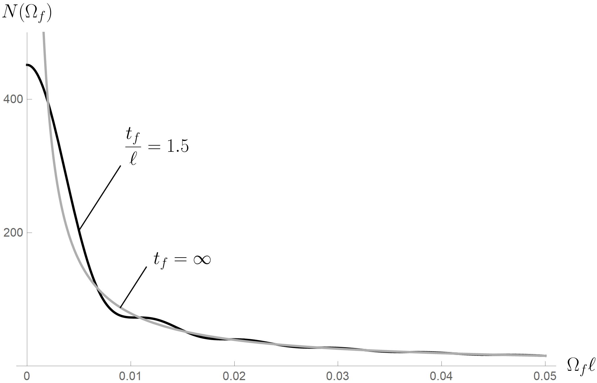
Figure 1: The spectrum of the occupation number is plotted with respect to the dimensionless frequency $\Omega_{f}\ell$ for two different times. The black and grey curves are for a finite time (44) ($t_{f}/\ell=1.5$) and for infinite time (46), respectively. Although the spectrum for the finite time is damped oscillating, the spectrum turns out to be approximately thermal for $t_{f}\to\infty$ when the shell approaches the horizon.

Note that the functional Schrödinger equation (20) tells us that the wave function is apparently responsible for the exterior and interior geometries through Eq. (16); however, the occupation number $N(t_{f},\Omega_{f})$ in the incipient limit is of no relevance to the interior geometry because $x$ and $z$ are independent of $f_{\rm in}$ as seen from Eq. (45). For the asymptotic observer, the shell does not collapse to $R_{H}$ in a finite time, but the collapsing shell takes infinite time to reach $R_{H}$. So, we should take the limit of $t_{f}\to\infty$ to study the quantum radiation when the black hole forms. For $t_{f}\to\infty$, we finally obtain the occupation number (44) as

$$N_{\infty}(z)=\frac{\pi}{8}\frac{z}{J_{1}^{2}(z)+Y_{1}^{2}(z)}\left[\left(J_{1}^{2}(z)+Y_{1}^{2}(z)-\frac{2}{\pi z}\right)^{2}+\left(J_{0}(z)J_{1}(z)+Y_{0}(z)Y_{1}(z)\right)^{2}\right],$$ (46)

where we used the following asymptotic forms of Bessel functions

$$\dfrac{x}{z}\left(\xi^{2}+\chi^{2}\right)\to\dfrac{\pi z}{2}\left(J_{1}^{2}(z)+Y_{1}^{2}(z)\right),$$ (47)

$$\dfrac{\xi\xi_{\hat{\eta}}+\chi\chi_{\hat{\eta}}}{x}\to-\dfrac{\pi z}{4}\left(J_{0}(z)J_{1}(z)+Y_{0}(z)Y_{1}(z)\right).$$ (48)

For convenience, the spectrum of the occupation number is plotted in Fig. 1. In a finite time, the radiation is nonthermal since the spectrum is quite different from the Planckian distribution. When the time goes to infinity, the spectrum approaches the Planckian distribution. In particular, in a low frequency region, Eq. (46) is written as

$$N_{\infty}(\Omega_{f})\approx\frac{f^{\prime}_{\rm out}(R_{H})}{4\pi\Omega_{f}}=\frac{\sqrt{M_{\rm out}}}{2\pi\ell~{}\Omega_{f}}.$$ (49)

Hence, the temperature of the quantum radiation can be read off from Eq. (49) by comparing it to the Planckian distribution in a low frequency as

$$T=\frac{\sqrt{M_{\rm out}}}{2\pi\ell}.$$ (50)

For $M_{\rm out}>0$ and $M_{\rm in}=0$, the present analytic account is compatible with the numerical result Saini:2017mur that the temperature of the emitted radiation is very close to the Hawking temperature as the shell approaches its own horizon. Of course, Eq. (50) is also valid for $M_{\rm out}>0$ and $M_{\rm in}=-1$.

IV conclusion and discussion

In conclusion, we considered the collapsing dust shell where the exterior and interior regions of the shell were described by the AdS geometry characterized by the different exterior and interior mass parameters of $M_{\rm out}$ and $M_{\rm in}$, and studied the quantum radiation from the collapsing shell by using the functional Schrödinger formalism. In the formation of the BTZ black hole where $M_{\rm out}>0$ and $M_{\rm in}=0,-1$, the wave function in the incipient BTZ black hole limit was fortunately expressed by the analytic form and so the occupation number of the excited states was calculated exactly. The spectrum of the occupation number is nonthermal for a finite time, but it is getting close to the thermal Hawking radiation as time goes to infinity.

Until now, we have studied the collapse of the BTZ black hole for which $M_{\rm out}>0$. Let us speculate what happens for the collapse where $M_{\rm out}<0$. As a matter of fact, for $-1<M_{\rm out}<0$, the end points of collapse depend on the initial velocity and position, and can lead to a naked singularity Peleg:1994wx ; Crisostomo:2003xz ; Mann:2006yu . To evade the naked singularity attributed to the exterior geometry, we can instead consider the collapse of the global AdS space as a thermal soliton of $M_{\rm out}=-1$ without the horizon. Firstly, assuming that the surface energy density $\sigma$ of the shell is positive in the formation of the global AdS space, then the interior mass parameter should be chosen as $M_{\rm in}<-1$ from Eq. (7) so that the interior geometry leads necessarily to the naked singularity. Of course, if the surface energy density is negative, then the interior mass parameter can be $M_{\rm in}=0$ for a particular value of $\mu$ where $\mu$ is the constant of motion defined by $\mu=2\pi R\sigma$; however, the negative energy density would be unnatural in the classical collapse. Secondly, the spectrum of the occupation number will appear to be nonthermal at very late times when the radius of the shell shrinks to $R\to 0$. This fact might be expected from the previous work for the collapse of a regular black hole in the absence of the horizon Um:2019qgc . Eventually, the occupation number would not be well-defined when encountering the naked singularity, which deserves further study.

- (1) S. W. Hawking, Particle Creation by Black Holes, Commun. Math. Phys. 43 (1975) 199–220.
- (2) J. B. Hartle and S. W. Hawking, Path Integral Derivation of Black Hole Radiance, Phys. Rev. D 13 (1976) 2188–2203.
- (3) G. W. Gibbons and S. W. Hawking, Cosmological Event Horizons, Thermodynamics, and Particle Creation, Phys. Rev. D 15 (1977) 2738–2751.
- (4) E. T. Akhmedov, H. Godazgar and F. K. Popov, Hawking radiation and secularly growing loop corrections, Phys. Rev. D 93 (2016) 024029, [1508.07500].
- (5) D. G. Boulware, Hawking Radiation and Thin Shells, Phys. Rev. D 13 (1976) 2169.
- (6) U. H. Gerlach, The Mechanism of Black Body Radiation from an Incipient Black Hole, Phys. Rev. D 14 (1976) 1479–1508.
- (7) K. Shizume and S. Takagi, Hawking Radiation Due to a Collapsing Star. II: Collapsing Shells in Two-Dimensional Space-Times, Progress of Theoretical Physics 81 (04, 1989) 826–840, [https://academic.oup.com/ptp/article-pdf/81/4/826/5257312/81-4-826.pdf].
- (8) G. L. Alberghi, R. Casadio, G. P. Vacca and G. Venturi, Gravitational collapse of a shell of quantized matter, Class. Quant. Grav. 16 (1999) 131–147, [gr-qc/9808026].
- (9) G. L. Alberghi, R. Casadio, G. P. Vacca and G. Venturi, Gravitational collapse of a radiating shell, Phys. Rev. D 64 (2001) 104012, [gr-qc/0102014].
- (10) R. B. Mann and S. F. Ross, Matching conditions and gravitational collapse in two-dimensional gravity, Class. Quant. Grav. 9 (1992) 2335–2350, [hep-th/9205098].
- (11) S. F. Ross and R. B. Mann, Gravitationally collapsing dust in (2+1)-dimensions, Phys. Rev. D 47 (1993) 3319–3322, [hep-th/9208036].
- (12) Y. Peleg and A. R. Steif, Phase transition for gravitationally collapsing dust shells in (2+1)-dimensions, Phys. Rev. D 51 (1995) 3992–3996, [gr-qc/9412023].
- (13) J. Crisostomo and R. Olea, Hamiltonian treatment of the gravitational collapse of thin shells, Phys. Rev. D 69 (2004) 104023, [hep-th/0311054].
- (14) R. B. Mann and J. J. Oh, Gravitationally Collapsing Shells in (2+1) Dimensions, Phys. Rev. D 74 (2006) 124016, [gr-qc/0609094].
- (15) S. Hyun, J. Jeong, W. Kim and J. J. Oh, Formation of Three-Dimensional Black Strings from Gravitational Collapse of Dust Cloud, JHEP 04 (2007) 088, [gr-qc/0612094].
- (16) T. Vachaspati, D. Stojkovic and L. M. Krauss, Observation of incipient black holes and the information loss problem, Phys. Rev. D76 (2007) 024005, [gr-qc/0609024].
- (17) T. Vachaspati and D. Stojkovic, Quantum radiation from quantum gravitational collapse, Phys. Lett. B 663 (2008) 107–110, [gr-qc/0701096].
- (18) E. Greenwood and D. Stojkovic, Hawking radiation as seen by an infalling observer, JHEP 09 (2009) 058, [0806.0628].
- (19) E. Greenwood, D. I. Podolsky and G. D. Starkman, Pre-Hawking Radiation from a Collapsing Shell, JCAP 1111 (2011) 024, [1011.2219].
- (20) M. Kolopanis and T. Vachaspati, Quantum Excitations in Time-Dependent Backgrounds, Phys. Rev. D87 (2013) 085041, [1302.1449].
- (21) A. Saini and D. Stojkovic, Radiation from a collapsing object is manifestly unitary, Phys. Rev. Lett. 114 (2015) 111301, [1503.01487].
- (22) A. Saini and D. Stojkovic, Hawking-like radiation and the density matrix for an infalling observer during gravitational collapse, Phys. Rev. D94 (2016) 064028, [1609.06584].
- (23) C. Kiefer, Functional Schrodinger equation for scalar QED, Phys. Rev. D 45 (1992) 2044–2056.
- (24) E. Greenwood, Hawking Radiation from a Reisner-Nordstrom Domain Wall, JCAP 01 (2010) 002, [0910.0024].
- (25) A. Das and N. Banerjee, Unitarity in Reissner–Nordström background: striding away from information loss, Eur. Phys. J. C79 (2019) 475, [1902.03378].
- (26) E. Greenwood, E. Halstead and P. Hao, Classical and Quantum Equations of Motion for a BTZ Black String in AdS Space, JHEP 02 (2010) 044, [0912.1860].
- (27) A. Saini and D. Stojkovic, Gravitational collapse and Hawking-like radiation of a shell in AdS spacetime, Phys. Rev. D97 (2018) 025020, [1711.08182].
- (28) H. Um and W. Kim, Formation of the Hayward black hole from a collapsing shell, Phys. Rev. D 101 (2020) 065017, [1912.04490].
- (29) M. Banados, C. Teitelboim and J. Zanelli, The Black hole in three-dimensional space-time, Phys. Rev. Lett. 69 (1992) 1849–1851, [hep-th/9204099].
- (30) W. Israel, Singular hypersurfaces and thin shells in general relativity, Nuovo Cim. B44S10 (1966) 1.
- (31) A. Edery, Non-singular vortices with positive mass in 2+1 dimensional Einstein gravity with AdS3 and Minkowski background, JHEP 01 (2021) 166, [2004.09295].
- (32) H. Goldstein, Classical Mechanics. Addison-Wesley, 1980.
- (33) C. M. A. Dantas, I. A. Pedrosa and B. Baseia, Harmonic oscillator with time-dependent mass and frequency and a perturbative potential, Phys. Rev. A45 (1992) 1320–1324.
- (34) M. Abramowitz, Handbook of Mathematical Functions, With Formulas, Graphs, and Mathematical Tables,. Dover Publications, Inc., USA, 1974.