Leveraging Non-uniformity in First-order Non-convex Optimization

Abstract

Classical global convergence results for first-order methods rely on uniform smoothness and the Łojasiewicz inequality. Motivated by properties of objective functions that arise in machine learning, we propose a non-uniform refinement of these notions, leading to Non-uniform Smoothness (NS) and Non-uniform Łojasiewicz inequality (NŁ). The new definitions inspire new geometry-aware first-order methods that are able to converge to global optimality faster than the classical $\Omega(1/t^{2})$ lower bounds. To illustrate the power of these geometry-aware methods and their corresponding non-uniform analysis, we consider two important problems in machine learning: policy gradient optimization in reinforcement learning (PG), and generalized linear model training in supervised learning (GLM). For PG, we find that normalizing the gradient ascent method can accelerate convergence to $O(e^{-c\cdot t})$ (where $c>0$) while incurring less overhead than existing algorithms. For GLM, we show that geometry-aware normalized gradient descent can also achieve a linear convergence rate, which significantly improves the best known results. We additionally show that the proposed geometry-aware gradient descent methods escape landscape plateaus faster than standard gradient descent. Experimental results are used to illustrate and complement the theoretical findings.

1 Introduction

The optimization of non-convex objective functions is a topic of key interest in modern-day machine learning. Recent, intriguing results show that simple gradient-based optimization can achieve globally optimal solutions in certain non-convex problems arising in machine learning, such as in reinforcement learning (RL) (Agarwal et al., 2020), supervised learning (SL) (Hazan et al., 2015), and deep learning (Allen-Zhu et al., 2019). While gradient-based algorithms remain the method of choice in machine learning, the convergence of such algorithms to global minimizers has still only been established in restrictive settings where one can assert two strong assumptions about the objective function: (1) that the objective is smooth, and (2) that the objective satisfies a gradient dominance over sub-optimality such as the Łojasiewicz inequality. We will find it beneficial to recall the definitions of these properties. For the remainder of this paper let $\Theta=\mathbb{R}^{d}$.

Definition 1 (Smoothness).

The function $f:\Theta\to{\mathbb{R}}$ is $\beta$-smooth ($\beta>0$) if it is differentiable and for all $\theta,\theta^{\prime}\in\Theta$,

$$\left|f(\theta^{\prime})-f(\theta)-\Big{\langle}\frac{df(\theta)}{d\theta},\theta^{\prime}-\theta\Big{\rangle}\right|\leq\frac{\beta}{2}\cdot\|\theta^{\prime}-\theta\|_{2}^{2}.$$ (1)

Definition 2.

(Łojasiewicz, 1963; Polyak, 1963; Kurdyka, 1998) The differentiable function $f:\Theta\to{\mathbb{R}}$ satisfies the $(C,\xi)$-Łojasiewicz inequality if for all $\theta\in\Theta$,

$$\left\|\frac{df(\theta)}{d\theta}\right\|_{2}\geq C\cdot\Big{(}f(\theta)-\inf_{\theta\in\Theta}{f(\theta)}\Big{)}^{1-\xi},$$ (2)

where $C>0$ and $\xi\in[0,1]$.

In particular, if an objective function $f$ satisfies both assumptions, gradient-based optimization can be shown to converge to a global minimizer by noting first that uniform smoothness Eq. 1 ensures the gradient updates achieve monotonic improvement with an appropriate step size (i.e., $f(\theta_{t+1})\leq f(\theta_{t})-\frac{1}{2\beta}\cdot\left\|\nabla f(\theta_{t})\right\|_{2}^{2}$, if $\theta_{t+1}\leftarrow\theta_{t}-\frac{1}{\beta}\cdot\nabla f(\theta_{t})$), while the Łojasiewicz inequality Eq. 2 ensures the gradient does not vanish before a global minimizer is reached. Several global convergence results have recently been achieved in the machine learning literature by exploiting assumptions of this kind. For example, in reinforcement learning it has recently been shown that policy gradient (PG) methods converge to a globally optimal policy (Agarwal et al., 2020; Mei et al., 2020b); in supervised learning it has been shown that gradient descent (GD) methods converge to global minimizers of certain non-convex problems (Hazan et al., 2015); and in deep learning theory it has been shown that (stochastic) GD can converge to a global minimizer with an over-parameterized neural network (Allen-Zhu et al., 2019).

However, previous work that relies on the two uniform conditions in Definitions 1 and 2 assumes universal constants $\beta$ and $C$, which ignores important problem structure and limits both the applicability of the results and the strength of the results that can be obtained.

In this paper, we expand the class of problems for which gradient-based optimization is globally convergent, develop novel gradient-based methods that better exploit local structure, and improve the convergence rate analysis. We achieve these results by first defining then investigating a new set of non-uniform smoothness and Łojasiewicz inequalities, which generalize the classical definitions and allow a refined characterization of the space of objectives. Given these refined notions, we then tailor novel gradient-based algorithms that improve previous methods for these new problem classes, and extend the analysis to exploit these new forms of non-uniformity, achieving significantly stronger convergence rates in many cases. Importantly, these improvements are achieved in non-convex optimization problems that arise in relevant machine learning problems.

The remainder of the paper is organized as follows. First, in Section 2 we illustrate how natural optimization problems, including those in machine learning, exhibit interesting local structure that cannot be adequately captured by the uniform smoothness and Łojasiewicz inequalities. Then, Section 3 introduces the the Non-uniform Smoothness (NS) property and the Non-uniform Łojasiewicz (NŁ) inequality, based on which Section 4 provides non-uniform analyses. Sections 5 and 6 then present new results for policy gradient and generalized linear models respectively. Section 7 concludes the paper and discusses some future directions. Due to space limits, we relegate most of the proofs to the appendix.

2 Motivation

To illustrate the significance of non-uniformity in machine learning problems, we consider examples motivated by recent theoretical (Zhang et al., 2019; Wilson et al., 2019; Mei et al., 2020b) and empirical studies (Cohen et al., 2021).

Regarding smoothness, it is clear that a uniform smoothness constant $\beta$ cannot always adequately characterize an objective over its entire domain. For example, the convex function $f:x\mapsto x^{4}$ cannot be informatively characterized by a uniform smoothness constant $\beta$ because its Hessian $f^{\prime\prime}:x\mapsto 12\cdot x^{2}$ has the property that $f^{\prime\prime}(x)\to\infty$ as $|x|\to\infty$, and $f^{\prime\prime}(x)\to 0$ as $|x|\to 0$. Varying smoothness of this kind has motivated the study of alternative definitions to explain, for example, the effectiveness of gradient clipping in training neural networks and normalization in optimization (Zhang et al., 2019; Wilson et al., 2019). Meanwhile Cohen et al. (2021) present neural network training results that cannot be well explained using the standard smoothness condition of Definition 1.

Regarding the Łojasiewicz inequality, a recent study of policy gradient optimization in reinforcement learning has shown that, with the standard softmax parameterization, the expected return objective cannot satisfy any Łojasiewicz inequality with a universal constant $C$ (Mei et al., 2020b), which removes the possibility of using Definition 2 to prove convergence. By introducing a non-uniform version of the Łojasiewicz inequality, the same authors were able to show a global convergence rate for the same problem.

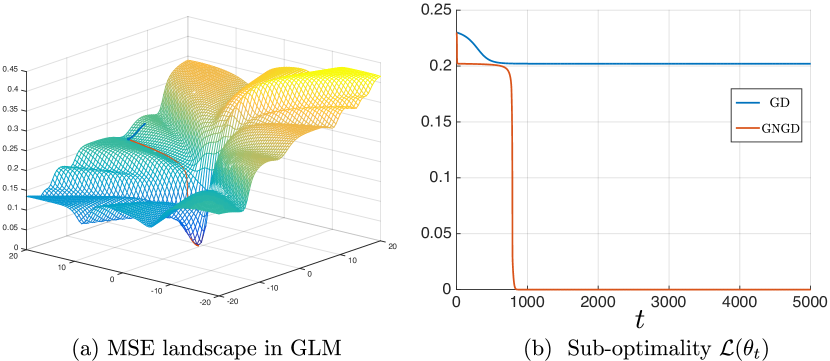
Figure 1: Non-uniform landscape of non-convex function.

Figure 1 illustrates another example of a non-convex objective, which arises in supervised learning. Subfigure 1(a) visualizes the mean squared error (MSE) of a generalized linear model (GLM) (Hazan et al., 2015), which is not only non-convex but also highly non-uniform. As a “teaser”, subfigure 1(b) compares the convergence behavior of two algorithms: standard gradient descent (GD), which suffers from slow convergence on the plateaus due to the non-uniformity of the objective, and an alternative algorithm (GNGD), soon to be introduced. This figure previews how proper handling of non-uniformity in the optimization landscape can enable significant acceleration of optimization progress, including a quick escape from plateaus.

3 Non-uniform Properties and Algorithms

The main results in this paper depend on two core concepts, Non-uniform Smoothness (NS) and Non-uniform Łojasiewicz (NŁ) inequality. The NS property is a new, intuitive generalization of smoothness. The NŁ inequality is a recent proposal of Mei et al. (2020b) and generalizes previous Łojasiewicz inequalities. Our key contribution is to show that the combination of these two non-uniform concepts is particularly powerful, applicable to important non-convex objectives in machine learning, and allows the development of improved algorithms and analysis.

3.1 Non-uniform Smoothness

The first main concept we leverage is a generalized notion of smoothness that depends on the parameters non-uniformly.

Definition 3 (Non-uniform Smoothness (NS)).

The function $f:\Theta\to{\mathbb{R}}$ satisfies $\beta(\theta)$ non-uniform smoothness if $f$ is differentiable and for all $\theta,\theta^{\prime}\in\Theta$,

$$\left|f(\theta^{\prime})-f(\theta)-\Big{\langle}\frac{df(\theta)}{d\theta},\theta^{\prime}-\theta\Big{\rangle}\right|\leq\frac{{\color[rgb]{1,0,0}\beta(\theta)}}{2}\cdot\|\theta^{\prime}-\theta\|_{2}^{2},$$

where $\beta$ is a positive valued function: $\beta:\Theta\to(0,\infty)$.

We will refer to $\beta(\theta)$ in Definition 3 as the NS coefficient. This alternative definition generalizes and unifies several smoothness concepts from the recent literature. First, NS clearly reduces to Eq. 1 with $\beta(\theta)=\beta$. However, NS also generalizes the notion of $(L_{0},L_{1})$ smoothness from Zhang et al. (2019) by using $\beta(\theta)=L_{0}+L_{1}\cdot\left\|\nabla f(\theta)\right\|_{2}$. By using $\beta(\theta)=c\cdot\left\|\nabla f(\theta)\right\|_{2}^{\frac{p-2}{p-1}}$, NS also reduces to the notion of strong smoothness of order $p$ proposed in Wilson et al. (2019). Finally, with $\beta(\theta)=c/\left\|\theta\right\|_{p}^{2}$, NS reduces to a special form of non-uniform smoothness considered in Mei et al. (2020a). We will show later that NS also covers other previously unstudied smoothness variants. Below we will demonstrate the key benefits of Definition 3 in terms of its generality, better convergence results, and practical implications in conjunction with the NŁ inequality.

3.2 Non-uniform Łojasiewicz Inequality

The second main concept we leverage is a generalized Łojasiewicz inequality introduced by Mei et al. (2020b):

Definition 4 (Non-uniform Łojasiewicz (NŁ)).

The differentiable function $f:\Theta\to{\mathbb{R}}$ satisfies the $(C(\theta),\xi)$ non-uniform Łojasiewicz inequality if for all $\theta\in\Theta$,

$$\left\|\frac{df(\theta)}{d\theta}\right\|_{2}\geq{\color[rgb]{1,0,0}C(\theta)}\cdot\left|f(\theta)-f(\theta^{*})\right|^{1-\xi},$$ (3)

where $\xi\in(-\infty,1]$, and $C(\theta):\Theta\to{\mathbb{R}}>0$ holds for all $\theta\in\Theta$. In this definition, either $\theta^{*}=\arg\min_{\theta\in\Theta}f(\theta)$, or $f(\theta^{*})$ is replaced with $\inf_{\theta}{f(\theta)}$ if the global optimum is not achieved within the domain $\Theta$.

Definition 4 extends the classical “uniform” Łojasiewicz inequalities in optimization literature, such as the Polyak-Łojasiewicz (PŁ) inequality with $C(\theta)=C>0$ and $\xi=1/2$ (Łojasiewicz, 1963; Polyak, 1963); and the Kurdyka-Łojasiewicz (KŁ) inequality by setting $C(\theta)=C>0$ (Kurdyka, 1998). Following (Mei et al., 2020b, a), we refer to $\xi$ as the NŁ degree and $C(\theta)$ as the NŁ coefficient. Generally speaking, a larger NŁ degree $\xi$ and NŁ coefficient $C(\theta)$ indicate faster convergence for gradient based algorithms. Appendix E provides an overview of remarkable non-convex functions that satisfy the NŁ inequality for various $\xi$ and $C(\theta)$. As stated, our main contribution in this paper is to show how, when combined with NS, NŁ becomes a powerful tool for both algorithm design and analysis, which is a novel direction of investigation.

3.3 Geometry-aware Gradient Descent

A key benefit of the non-uniform definitions is that we can introduce stepsize rules that make gradient descent adapt to the local “geometry” of the optimization objective. First consider the classical gradient decent update.

Definition 5 (Gradient Descent (GD)).

$$\theta_{t+1}\leftarrow\theta_{t}-\eta\cdot\nabla f(\theta_{t}).$$ (4)

The key challenge with deploying GD is choosing the step size $\eta$; if $\eta$ is too large, instability ensues, if too small, progress becomes slow. Recall from the introduction that $\eta=1/\beta$ is a canonical choice for assuring convergence in uniformly $\beta$ smooth objectives. This suggests that in the presence of non-uniform smoothness $\beta(\theta)$ given in NS, the stepsize should be adapted to $1/\beta(\theta)$. This leads to a new variant of normalized gradient descent.

Definition 6 (Geometry-aware Normalized GD (GNGD)).

$$\theta_{t+1}\leftarrow\theta_{t}-\eta\cdot\frac{\nabla f(\theta_{t})}{\color[rgb]{1,0,0}{\beta(\theta_{t})}}.$$ (5)

Key to making this approach practical will be efficient ways to measure (or bound) $\beta(\theta)$. Below we will show how in the context of NS and NŁ properties, GNGD can be made both practical and extremely efficient at solving various global optimization problems in machine learning. These results also broaden our fundamental knowledge of the set of objectives that admit efficient global optimization.

4 Non-uniform Analysis

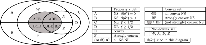
Figure 2: Different function classes for $\beta(\theta^{*})<\infty$. We use a label notation where, e.g., C denotes the set of all functions that satisfy property C, and $\text{ACE}\coloneqq\text{A}\cap\text{C}\cap\text{E}$. The two largest ellipsoids correspond to $\text{A}\cup\text{B}$ and C. We study the following four non-convex function classes in $(\text{A}\cup\text{B})\cap C$, i.e., ${\mathcal{W}}\coloneqq\text{AC}\setminus(\text{AD}\cup\text{ACE})$, ${\mathcal{X}}\coloneqq\text{AD}\setminus\text{ADE}$, ${\mathcal{Y}}\coloneqq\text{BC}\setminus(\text{BD}\cup\text{BCE})$, and ${\mathcal{Z}}\coloneqq\text{BD}\setminus(\text{BDE}\cup\text{BF})$.

Our first main contribution is an analysis for GD and GNGD based in the presence of non-uniform properties. For minimization problems, we assume $\inf_{\theta}{f(\theta)}>-\infty$ ($\sup_{\theta}{f(\theta)}<\infty$ for maximization problems).

Theorem 1.

Suppose $f:\Theta\to{\mathbb{R}}$ satisfies NS with $\beta(\theta)$ and the NŁ inequality with $(C(\theta),\xi)$. Suppose $C\coloneqq\inf_{t\geq 1}{C(\theta_{t})}>0$ for GD and GNGD. Let $\delta(\theta)\coloneqq f(\theta)-f(\theta^{*})$ be the sub-optimality gap. The following hold:

(1a)

if $\beta(\theta)\leq c\cdot\delta(\theta)^{1-2\xi}$ with $\xi\in(-\infty,1/2)$, then the conclusions of (1b) hold;

(1b)

if $\beta(\theta)\leq c\cdot\left\|\nabla f(\theta)\right\|_{2}^{\frac{1-2\xi}{1-\xi}}$ with $\xi\in(-\infty,1/2)$, then GD with $\eta\in O(1)$ achieves $\delta(\theta_{t})\in\Theta(1/t^{\frac{1}{1-2\xi}})$, and GNGD achieves $\delta(\theta_{t})\in O(e^{-t})$.

(2a)

if $\beta(\theta)\leq L_{0}+L_{1}\cdot\left\|\nabla f(\theta)\right\|_{2}$, then the conclusions of (2b) hold;

(2b)

if $\beta(\theta)\leq L_{0}\cdot\frac{\left\|\nabla f(\theta)\right\|^{2}}{\delta(\theta)^{2-2\xi}}+L_{1}\cdot\left\|\nabla f(\theta)\right\|_{2}$, then GD and GNGD both achieve $\delta(\theta_{t})\in O(1/t^{\frac{1}{1-2\xi}})$ when $\xi\in(-\infty,1/2)$, and $O(e^{-t})$ when $\xi=1/2$. GNGD has strictly better constant than GD ($1>C>C^{2}$).

(3a)

if $\beta(\theta)\!\leq\!c\!\cdot\!\left\|\nabla f(\theta)\right\|_{2}^{\frac{1-2\xi}{1-\xi}}\!$ with $\xi\in(1/2,1)$, then the conclusions of (3b) hold;

(3b)

if $\beta(\theta)\leq c\cdot\delta(\theta)^{1-2\xi}$ with $\xi\in(1/2,1)$, then GD with $\eta\in\Theta(1)$ does not converge, while GNGD achieves $\delta(\theta_{t})\in O(e^{-t})$.

Remark 1.

The cases (1)-(3) cover all three possibilities of $\beta(\theta^{*})$. Since $\theta^{*}$ is the global minimum, $\nabla^{2}f(\theta^{*})$ is positive semi-definite (negative if $\theta^{*}$ is maximum) if it exists.

• If $\nabla^{2}f(\theta^{*})={\mathbf{0}}$, then $\beta(\theta)\to 0$ as $\theta,\theta^{\prime}\to\theta^{*}$, which means the landscape around $\theta^{*}$ is flat;

• If $\nabla^{2}f(\theta^{*})$ has at least one strictly positive (negative) eigenvalue, then $\beta(\theta)\to\beta>0$ as $\theta,\theta^{\prime}\to\theta^{*}$.

The cases (1)-(2) also cover the situations where the Hessian $\nabla^{2}f(\theta^{*})$ does not exist but one can find a finite $\beta(\theta^{*})>0$ to upper bound the l.h.s. of Definition 3.

• The case (3) is for blow-up type non-existence of $\nabla^{2}f(\theta^{*})$, where $\beta(\theta^{*})$ is unbounded.

Remark 2.

In Theorem 1, $C\coloneqq\inf_{t\geq 1}{C(\theta_{t})}$ is related to the early optimization and plateau escaping behavior studied in Mei et al. (2020a). It remains open to study whether GNGD can be combined with different parameterizations in Mei et al. (2020a) to further improve $C$.

Note that (1b) recovers the strong smoothness of order $p$ with $p=1/\xi$ in Wilson et al. (2019), and (2a) recovers the $(L_{0},L_{1})$ smoothness of Zhang et al. (2019). The results here consider more general NŁ functions and establish faster rates of convergence. The other cases have not been studied in literature to our knowledge. In Sections 5 and 6 below we study practical machine learning examples that are covered by cases (1) and (2) in Theorem 1. Other cases of different $\beta(\theta)$ and $\xi$ are discussed in Appendix A for completeness.

4.1 Function Classes and Existing Lower Bounds

Before applying these results to problems in machine learning, we first provide a refined characterization of function classes organized by their NS and NŁ properties. This also clarifies the relation between the non-uniform properties and standard notions of convexity and smoothness; see Figure 2.

Proposition 1.

The following hold for an objective $f$:

• $\text{D}\subseteq\text{C}$. If $f$ satisfies NŁ with degree $\xi$, it satisfies NŁ with degree $\xi^{\prime}<\xi$;

• $\text{F}\!\subseteq\!\text{D}$. A strongly convex $f$ satisfies NŁ with $\xi\!=\!1/2$;

• $\text{F}\cap\text{A}=\emptyset$. A strongly convex $f$ cannot satisfy NS with $\beta(\theta)\to 0$ as $\theta,\theta^{\prime}\to\theta^{*}$;

• $\text{E}\!\subseteq\!\text{C}$. A (not strongly) convex $f$ satisfies NŁ with $\xi\!=\!0$.

The next proposition provides concrete examples for each convex function class in $(A\cup B)\cap C$ in Figure 2.

Proposition 2.

The following results hold: (1) $\text{ACE}\not=\emptyset$. (2) $\text{ADE}\not=\emptyset$. (3) $\text{BCE}\not=\emptyset$. (4) $\text{BDE}\not=\emptyset$. (5) $\text{BF}\not=\emptyset$.

A more interesting result considers examples in the classes of non-convex functions $(A\cup B)\cap C$ in Figure 2. The non-uniform analysis above largely still applies to these problems, even when standard convex analysis cannot apply.

Proposition 3.

The following results hold: (1) ${\mathcal{W}}\coloneqq\text{AC}\setminus(\text{AD}\cup\text{ACE})\not=\emptyset$. (2) ${\mathcal{X}}\coloneqq\text{AD}\setminus\text{ADE}\not=\emptyset$. (3) ${\mathcal{Y}}\coloneqq\text{BC}\setminus(\text{BD}\cup\text{BCE})\not=\emptyset$. (4) ${\mathcal{Z}}\coloneqq\text{BD}\setminus(\text{BDE}\cup\text{BF})\not=\emptyset$.

We next apply the techniques to a class of convex functions, achieving results that cannot be explained by classical convex-smooth analysis.

Proposition 4.

The convex function $f:x\mapsto|x|^{p}$ with $p>1$ satisfies the NŁ inequality with $\xi=1/p$ and the NS property with $\beta(x)\leq c_{1}\cdot\delta(x)^{1-2\xi}$.

Consider any $p>2$, such as $p=4$, where it follows that $f$ satisfies NŁ with degree $\xi=1/4<1/2$. According to (1a) in Theorem 1, GD will achieve $\delta(x_{t})\in\Theta(1/t^{2})$, while GNGD attains $\delta(x_{t})\in O(e^{-c\cdot t})$ (where $c>0$). Note that standard convex analysis can only give a $O(1/t)$ rate on (not strongly) convex smooth functions. The $\Theta(1/t^{2})$ rate for GD here follows from using NŁ degree $\xi=1/4$, which improves on $\xi=0$ from mere convexity ((4) in Proposition 1). The $O(e^{-c\cdot t})$ rate has also been observed for this example by exploiting strong smoothness ((1b), as noted) (Wilson et al., 2019). Figure 2 provides a more general understanding of when this happens.

$\Omega(1/t^{2})$ lower bound for convexity-smoothness.

Note that GNGD satisfies $x_{t+1}=x_{1}-\sum_{i=1}^{t}{\frac{\eta}{\beta(x_{i})}\cdot\nabla f(x_{i})}\in\text{Span}\left\{x_{1},\nabla f(x_{1}),\dots,\nabla f(x_{t})\right\}$, which is a first-order oracle (Nesterov, 2003). Thus there exists a worst-case objective in the convex-smooth class that forces $\delta(x_{t})\in\Omega(1/t^{2})$ for $t\in O(n)$, where $n$ is the parameter dimension (Nemirovski & Yudin, 1983; Nesterov, 2003; Bubeck, 2014). This is not a contradiction, since the lower bound is established by constructing a convex smooth function with a constant $\beta>0$ (Bubeck, 2014), and $\beta(x)\to\beta>0$ as $x,x^{\prime}\to x^{*}$ in Definition 3. Hence, the $\Omega(1/t^{2})$ result covers some functions in BCE in Figure 2. Meanwhile $f:x\mapsto|x|^{p}$ with $p>2$ satisfies $\beta(x)\to 0$ as $x,x^{\prime}\to 0$ in Definition 3 (ACE in Figure 2), which implies that the standard convex-smooth class consists of two subclasses. One subclass (BCE) admits first-order sub-linear lower bounds, while the other (ACE) allows linear convergence using first-order methods. This illustrates the necessity of non-uniformity in subdividing the NS class as $\text{A}\cup\text{B}$ in Figure 2. This partition also inspires geometry-aware GD.

$\Omega(1/\sqrt{t})$ lower bound for $(L_{0},L_{1})$-smoothness.

For $\beta(\theta)=L_{0}+L_{1}\cdot\|\nabla f(\theta)\|_{2}$ ((2a) in Theorem 1) with $L_{0},L_{1}\geq 1$, standard normalized GD is subject to a $\Omega(1/\sqrt{t})$ lower bound (Zhang et al., 2019). However, in Section 5, we will show that normalized policy gradient (PG) method achieves a linear rate of $O(e^{-c\cdot t})$. Again, this is not a contradiction for similar reasons. With $L_{0}\geq 1$, $\beta(\theta)\to L_{0}>0$ as $\theta,\theta^{\prime}\to\theta^{*}$, the $\Omega(1/\sqrt{t})$ lower bound will hold for some functions in $\text{BCE}\cup{\mathcal{Y}}$ in Figure 2. While in Section 5 the objective satisfies $L_{0}=0$ and $L_{1}>0$, hence $\beta(\theta)\to 0$ as $\theta,\theta^{\prime}\to\theta^{*}$ ($\text{ACE}\cup{\mathcal{W}}$ in Figure 2). This shows a similar separation of rates for first-order methods will also occur based on NS conditions. Furthermore, in Section 6, we will show that both GD and GNGD achieve a $O(e^{-c\cdot t})$ rate for GLM, but here the objective is in ${\mathcal{Z}}$ in Figure 2 so the lower bounds do not apply.

Unbounded Hessian.

Consider any $p\in(1,2)$, such as $p=3/2$ where $f$ satisfies $\xi=2/3$. According to Theorem 1(3a), GD diverges since the Hessian is unbounded near $0$. This makes it necessary to introduce geometry-aware normalization to ensure convergence, which is verified in Appendix F. This has practical implications for RL, for example ensuring exploration using state distribution entropy, which has unbounded Hessian near probability simplex boundary (Hazan et al., 2019) and alternative probability transforms (Mei et al., 2020a).

5 Policy Gradient

Our second main contribution is to show that the expected return objective considered in direct policy optimization in RL falls under the function class ${\mathcal{W}}$ in Figure 2, in particular satisfying case (1) of Theorem 1 with NŁ degree $\xi=0$. The key point is that value functions in Markov decision processes (MDPs) satisfy NS properties with coefficient being the PG norm (Lemmas 2 and 6). This novel finding not only provides a much more precise characterization than existing standard smoothness results (Agarwal et al., 2020; Mei et al., 2020b), but also enables PG with normalization to use the NŁ inequalities (Lemmas 1 and 5) differently than for standard PG ($\left\|\nabla f(\theta)\right\|_{2}$ vs. $\left\|\nabla f(\theta)\right\|_{2}^{2}$), which leads to faster convergence as well as plateau escaping.

5.1 RL Settings and Notations

For a finite set ${\mathcal{N}}$, let $\Delta({\mathcal{N}})$ denote the set of all probability distributions on ${\mathcal{N}}$. A finite MDP ${\mathcal{M}}\coloneqq({\mathcal{S}},{\mathcal{A}},{\mathcal{P}},r,\gamma)$ is determined by a finite state space ${\mathcal{S}}$, a finite action space ${\mathcal{A}}$, a transition function ${\mathcal{P}}:{\mathcal{S}}\times{\mathcal{A}}\to\Delta({\mathcal{S}})$, a scalar reward function $r:{\mathcal{S}}\times{\mathcal{A}}\to{\mathbb{R}}$, and a discount factor $\gamma\in[0,1)$.

In policy-based RL, an agent interacts with the environment, i.e., the MDP ${\mathcal{M}}$, using a policy $\pi:{\mathcal{S}}\to\Delta({\mathcal{A}})$. Given a state $s_{t}$, the agent takes an action $a_{t}\sim\pi(\cdot|s_{t})$, receives a one-step scalar reward $r(s_{t},a_{t})$ and a next-state $s_{t+1}\sim{\mathcal{P}}(\cdot|s_{t},a_{t})$. The long-term expected reward, also known as the value function of $\pi$ under $s$, is defined as

$$V^{\pi}(s)\coloneqq\operatorname*{\mathbb{E}}_{\begin{subarray}{c}s_{0}=s,a_{t}\sim\pi(\cdot|s_{t}),\\ s_{t+1}\sim{\mathcal{P}}(\cdot|s_{t},a_{t})\end{subarray}}{\left[\sum_{t=0}^{\infty}{\gamma^{t}r(s_{t},a_{t})}\right]}.$$ (6)

The state-action value of $\pi$ at $(s,a)\in{\mathcal{S}}\times{\mathcal{A}}$ is defined as $Q^{\pi}(s,a)\coloneqq r(s,a)+\gamma\sum_{s^{\prime}}{{\mathcal{P}}(s^{\prime}|s,a)V^{\pi}(s^{\prime})}$, and $A^{\pi}(s,a)\coloneqq Q^{\pi}(s,a)-V^{\pi}(s)$ is the advantage function of $\pi$. The state distribution of $\pi$ is defined as,

$$d_{s_{0}}^{\pi}(s)\coloneqq(1-\gamma)\sum_{t=0}^{\infty}{\gamma^{t}\operatorname*{Pr}(s_{t}=s|s_{0},\pi,{\mathcal{P}})}.$$ (7)

Given an initial state distribution $\rho\in\Delta({\mathcal{S}})$, we denote $V^{\pi}(\rho)\coloneqq\operatorname*{\mathbb{E}}_{s\sim\rho}{\left[V^{\pi}(s)\right]}$ and $d_{\rho}^{\pi}(s)\coloneqq\operatorname*{\mathbb{E}}_{s_{0}\sim\rho}{\left[d_{s_{0}}^{\pi}(s)\right]}$. There exists an optimal policy $\pi^{*}$ such that $V^{\pi^{*}}(\rho)=\sup_{\pi:{\mathcal{S}}\to\Delta({\mathcal{A}})}{V^{\pi}(\rho)}$. For convenience, we denote $V^{*}\coloneqq V^{\pi^{*}}$. Consider a tabular representation, i.e., $\theta(s,a)\in{\mathbb{R}}$ for all $(s,a)$, so that the policy $\pi_{\theta}$ can be parameterized by $\theta$ as $\pi_{\theta}(\cdot|s)=\mathrm{softmax}(\theta(s,\cdot))$; that is, for all $(s,a)$,

$$\pi_{\theta}(a|s)=\frac{\exp\{\theta(s,a)\}}{\sum_{a^{\prime}\in{\mathcal{A}}}{\exp\{\theta(s,a^{\prime})\}}}.$$ (8)

When there is only one state the policy $\pi_{\theta}=\mathrm{softmax}(\theta)$ is defined as $\pi_{\theta}(a)=\exp\{\theta(a)\}/\sum_{a^{\prime}\in{\mathcal{A}}}{\exp\{\theta(a^{\prime})}$. The problem of policy-based RL is then to find a policy $\pi_{\theta}$ that maximizes the value function, i.e.,

$$\sup_{\theta:{\mathcal{S}}\times{\mathcal{A}}\to{\mathbb{R}}}{V^{\pi_{\theta}}(\rho)}.$$ (9)

For convenience, and without loss of generality, we assume $r(s,a)\in[0,1]$ for all $(s,a)\in{\mathcal{S}}\times{\mathcal{A}}$.

5.2 One-state MDPs

We first illustrate some key insights for one-state MDPs with $K$ actions and $\gamma=0$. The value function Eq. 6 reduces to expected reward $\pi_{\theta}^{\top}r$, where $r\in[0,1]^{K}$, $\theta\in{\mathbb{R}}^{K}$, and $\pi_{\theta}=\mathrm{softmax}(\theta)$. Mei et al. (2020b) have shown that even though $\max_{\theta}{\pi_{\theta}^{\top}r}$ is a non-concave maximization, global convergence can be achieved with a $O(1/t)$ rate using uniform smoothness and the NŁ inequality:

Lemma 1 (NŁ, Mei et al. (2020b), Lemma 3).

Let $a^{*}$ be the optimal action. Denote $\pi^{*}=\operatorname*{arg\,max}_{\pi\in\Delta}{\pi^{\top}r}$. Then,

$$\left\|\frac{d\pi_{\theta}^{\top}r}{d\theta}\right\|_{2}\geq\pi_{\theta}(a^{*})\cdot(\pi^{*}-\pi_{\theta})^{\top}r.$$ (10)

Note that Lemma 1 is not improvable in terms of the coefficients $C(\theta)=\pi_{\theta}(a^{*})$ and $\xi=0$ (Mei et al., 2020b, Remark 1 and Lemma 17). However, this result is based on only using a uniform smoothness coefficient $\beta=5/2$ (Mei et al., 2020b, Lemma 2), which even empirical evidence suggests can be significantly refined. To illustrate, we run standard policy gradient (PG) on a $3$-action one-state MDP. As shown in Figure 3(a), PG first goes through a long suboptimal plateau, and then eventually escapes to approach $\pi^{*}$. Figure 3(b) presents the spectral radius of the Hessian and the PG norm $3\cdot\Big{\|}\frac{d\pi_{\theta_{t}}^{\top}r}{d\theta_{t}}\Big{\|}_{2}$ as functions of time $t$. It is evident that the smoothness behaves non-uniformly: it is close to zero at the suboptimal plateau and near $\pi^{*}$, highly aligned with the PG norm. Compared to any universal constant $\beta$, the PG norm characterizes the non-uniform landscape information far more precisely. We formalize this observation by proving the following key result:

Lemma 2 (NS).

Denote $\theta_{\zeta}\coloneqq\theta+\zeta\cdot(\theta^{\prime}-\theta)$ with some $\zeta\in[0,1]$. For any $r\in\left[0,1\right]^{K}$, $\theta\mapsto\pi_{\theta}^{\top}r$ satisfies $\beta(\theta_{\zeta})$ non-uniform smoothness with $\beta(\theta_{\zeta})=3\cdot\Big{\|}\frac{d\pi_{\theta_{\zeta}}^{\top}r}{d{\theta_{\zeta}}}\Big{\|}_{2}$.

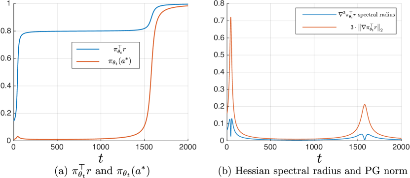
Figure 3: PG results on $r=(1.0,0.8,0.1)^{\top}$.

Comparing Lemma 2 with (1b) in Theorem 1, we have $\xi=0$, and GNGD requires normalizing $\beta(\theta_{\zeta})$, which is the PG norm of $\theta_{\zeta}$ rather than $\theta$. However, $\zeta$ is unknown. Fortunately, the next lemma shows that, if we still normalize the PG norm of $\theta$, the $\beta(\theta_{\zeta})$ in Lemma 2 can be upper bounded by $\Big{\|}\frac{d\pi_{\theta}^{\top}r}{d{\theta}}\Big{\|}_{2}$, given the learning rate is small enough:

Lemma 3.

Let $\theta^{\prime}=\theta+\eta\cdot\frac{d\pi_{\theta}^{\top}r}{d{\theta}}\Big{/}\left\|\frac{d\pi_{\theta}^{\top}r}{d{\theta}}\right\|_{2}$. Denote $\theta_{\zeta}\coloneqq\theta+\zeta\cdot(\theta^{\prime}-\theta)$ with some $\zeta\in[0,1]$. We have, for all $\eta\in(0,1/3)$,

$$\bigg{\|}\frac{d\pi_{\theta_{\zeta}}^{\top}r}{d{\theta_{\zeta}}}\bigg{\|}_{2}\leq\frac{1}{1-3\eta}\cdot\left\|\frac{d\pi_{\theta}^{\top}r}{d{\theta}}\right\|_{2}.$$ (11)

Next, the NŁ coefficient $\pi_{\theta}(a^{*})$ is bounded away from $0$, which provides constants in the convergence rate results.

Lemma 4 (Non-vanishing NŁ coefficient).

Using normalized policy gradient method, we have $\inf_{t\geq 1}\pi_{\theta_{t}}(a^{*})>0$.

To this point, we demonstrate that the non-concave function $\pi_{\theta}^{\top}r$ satisfies (1b) in Theorem 1 with $\xi=0$ in each iteration of normalized PG: Lemmas 2 and 3 show that the NS coefficient $\beta(\theta_{\zeta_{t}})\leq c_{1}\cdot\Big{\|}\frac{d\pi_{\theta_{t}}^{\top}r}{d{\theta_{t}}}\Big{\|}_{2}$, while Lemmas 1 and 4 guarantee $\Big{\|}\frac{d\pi_{\theta_{t}}^{\top}r}{d{\theta_{t}}}\Big{\|}_{2}\geq c_{2}\cdot(\pi^{*}-\pi_{\theta_{t}})^{\top}r$. Therefore, combining Lemmas 2, 1, 4 and 3, we prove the global linear convergence rate $O(e^{-c\cdot t})$ of normalized PG:

Theorem 2.

Using normalized PG $\theta_{t+1}=\theta_{t}+\eta\cdot\frac{d\pi_{\theta_{t}}^{\top}r}{d{\theta_{t}}}\Big{/}\Big{\|}\frac{d\pi_{\theta_{t}}^{\top}r}{d{\theta_{t}}}\Big{\|}_{2}$, with $\eta=1/6$, for all $t\geq 1$, we have,

$$(\pi^{*}-\pi_{\theta_{t}})^{\top}r\leq e^{-\frac{c\cdot(t-1)}{12}}\cdot\left(\pi^{*}-\pi_{\theta_{1}}\right)^{\top}r,$$ (12)

where $c=\inf_{t\geq 1}\pi_{\theta_{t}}(a^{*})>0$ is from Lemma 4, and $c$ is a constant that depends on $r$ and $\theta_{1}$, but not on the time $t$.

Remark 3.

If $\pi_{\theta_{1}}$ is uniform, i.e., $\pi_{\theta_{1}}(a)=1/K$, $\forall\ a\in[K]$, then we have $c\geq 1/K$ in Theorem 2. This can be proved by showing that $\pi_{\theta_{t+1}}(a^{*})\geq\pi_{\theta_{t}}(a^{*})$, similar to Mei et al. (2020b, Proposition 2).

5.3 Geometry-aware Normalized PG (GNPG)

Next, we generalize from one-state to finite MDPs, using the GNPG on value function, as shown in Algorithm 1.

Algorithm 1 Geometry-aware Normalized Policy Gradient

  Input: Learning rate $\eta>0$.

  Initialize parameter $\theta_{1}(s,a)$ for all $(s,a)$.

  while $t\geq 1$ do

     $\theta_{t+1}\leftarrow\theta_{t}+\eta\cdot\frac{\partial V^{\pi_{\theta_{t}}}(\mu)}{\partial\theta_{t}}\Big{/}\left\|\frac{\partial V^{\pi_{\theta_{t}}}(\mu)}{\partial\theta_{t}}\right\|_{2}$.

  end while

5.4 General MDPs

For general finite MDPs, we assume “sufficient exploration” for the initial state distribution $\mu$, which is also adapted in literature (Agarwal et al., 2020; Mei et al., 2020b).

Assumption 1 (Sufficient exploration).

The initial state distribution satisfies $\min_{s}\mu(s)>0$.

Given 1, Agarwal et al. (2020) prove asymptotic global convergence for PG on the non-concave $\max_{\theta}{V^{\pi_{\theta}}(\rho)}$ problem, while Mei et al. (2020b) strengthens this to a $O(1/t)$ rate using uniform smoothness and the following NŁ inequality that generalizes Lemma 1.

Lemma 5 (NŁ, Mei et al. (2020b), Lemma 8).

Denote $S\coloneqq|{\mathcal{S}}|$ as the total number of states. We have, $\forall\ \theta\in{\mathbb{R}}^{{\mathcal{S}}\times{\mathcal{A}}}$,

$$\left\|\frac{\partial V^{\pi_{\theta}}(\mu)}{\partial\theta}\right\|_{2}\geq\frac{\min_{s}{\pi_{\theta}(a^{*}(s)|s)}}{\sqrt{S}\cdot\left\|d_{\rho}^{\pi^{*}}/d_{\mu}^{\pi_{\theta}}\right\|_{\infty}}\cdot\left(V^{*}(\rho)-V^{\pi_{\theta}}(\rho)\right),$$

where $a^{*}(s)$ is the action that $\pi^{*}$ selects in state $s$.

Here, the NŁ degree $\xi=0$ is not improvable Mei et al. (2020b, Lemma 28). In one-state MDPs with $S=1$, Lemma 5 recovers Lemma 1 with the same NŁ coefficient $C(\theta)=\pi_{\theta}(a^{*})$, indicating that $C(\theta)$ in Lemma 5 might also be unimprovable. On the other hand, the uniform smoothness considered in (Agarwal et al., 2020; Mei et al., 2020b) $\beta=8/(1-\gamma)^{3}$ is too conservative, particularly when $\gamma$ is close to $1$. Our next key result shows that the policy value also satisfies a stronger NS property, with the NS coefficient being the PG norm, generalizing Lemma 2:

Lemma 6 (NS).

Let 1 hold and denote $\theta_{\zeta}\coloneqq\theta+\zeta\cdot(\theta^{\prime}-\theta)$ with some $\zeta\in[0,1]$. $\theta\mapsto V^{\pi_{\theta}}(\mu)$ satisfies $\beta(\theta_{\zeta})$ non-uniform smoothness with

$$\beta(\theta_{\zeta})=\left[3+\frac{4\cdot\left(C_{\infty}-(1-\gamma)\right)}{1-\gamma}\right]\cdot\sqrt{S}\cdot\left\|\frac{\partial V^{\pi_{\theta_{\zeta}}}(\mu)}{\partial{\theta_{\zeta}}}\right\|_{2},$$

where $C_{\infty}\coloneqq\max_{\pi}{\left\|\frac{d_{\mu}^{\pi}}{\mu}\right\|_{\infty}}\leq\frac{1}{\min_{s}\mu(s)}<\infty$.

In one-state MDPs with $\gamma=0$ and $S=1$, we have $C_{\infty}=1-\gamma$. Thus Lemma 6 reduces to Lemma 2 with the same NS coefficient $\beta(\theta_{\zeta})=3\cdot\Big{\|}\frac{d\pi_{\theta_{\zeta}}^{\top}r}{d{\theta_{\zeta}}}\Big{\|}_{2}$. Similar to Lemma 3, if we use Algorithm 1 with small enough learning rate, then $\beta(\theta_{\zeta})$ in Lemma 6 is upper bounded by the PG norm of $\theta$:

Lemma 7.

Let $\eta=\frac{1-\gamma}{6\cdot(1-\gamma)+8\cdot\left(C_{\infty}-(1-\gamma)\right)}\cdot\frac{1}{\sqrt{S}}$ and $\theta^{\prime}=\theta+\eta\cdot\frac{\partial V^{\pi_{\theta}}(\mu)}{\partial\theta}\Big{/}\left\|\frac{\partial V^{\pi_{\theta}}(\mu)}{\partial\theta}\right\|_{2}$. Denote $\theta_{\zeta}\coloneqq\theta+\zeta\cdot(\theta^{\prime}-\theta)$ with some $\zeta\in[0,1]$. We have,

$$\left\|\frac{\partial V^{\pi_{\theta_{\zeta}}}(\mu)}{\partial\theta_{\zeta}}\right\|_{2}\leq 2\cdot\left\|\frac{\partial V^{\pi_{\theta}}(\mu)}{\partial\theta}\right\|_{2}.$$ (13)

Next, the NŁ coefficient $\min_{s}{\pi_{\theta}(a^{*}(s)|s)}$ in Lemma 5 is lower bounded away from $0$:

Lemma 8 (Non-vanishing NŁ coefficient).

Let 1 hold. We have, $c:=\inf_{s\in\mathcal{S},t\geq 1}\pi_{\theta_{t}}(a^{*}(s)|s)>0$, where $\left\{\theta_{t}\right\}_{t\geq 1}$ is generated by Algorithm 1.

Now we have the non-concave function $V^{\pi_{\theta}}(\rho)$ satisfies (1b) in Theorem 1 with $\xi=0$ in each iteration of Algorithm 1. Therefore, combining Lemmas 6, 5, 8 and 7, we prove the global linear convergence rate $O(e^{-c\cdot t})$ of Algorithm 1:

Theorem 3.

Let 1 hold and let $\left\{\theta_{t}\right\}_{t\geq 1}$ be generated using Algorithm 1 with $\eta=\frac{1-\gamma}{6\cdot(1-\gamma)+8\cdot\left(C_{\infty}-(1-\gamma)\right)}\cdot\frac{1}{\sqrt{S}}$, where $C_{\infty}\coloneqq\max_{\pi}{\left\|\frac{d_{\mu}^{\pi}}{\mu}\right\|_{\infty}}$. Denote $C_{\infty}^{\prime}\coloneqq\max_{\pi}{\left\|\frac{d_{\rho}^{\pi}}{\mu}\right\|_{\infty}}$. Let $c$ be the positive constant from Lemma 8. We have, for all $t\geq 1$,

$$V^{*}(\rho)-V^{\pi_{\theta_{t}}}(\rho)\leq\frac{\left(V^{*}(\mu)-V^{\pi_{\theta_{1}}}(\mu)\right)\cdot C_{\infty}^{\prime}}{1-\gamma}\cdot e^{-C\cdot(t-1)},$$

where $C=\frac{(1-\gamma)^{2}\cdot c}{12\cdot(1-\gamma)+16\cdot\left(C_{\infty}-(1-\gamma)\right)}\cdot\frac{1}{S}\cdot\Big{\|}\frac{d_{\mu}^{\pi^{*}}}{\mu}\Big{\|}_{\infty}^{-1}$.

Not only the $O(e^{-c\cdot t})$ rate in Theorem 3 is faster than $O(1/t)$ for standard PG without normalization, but also the constant is better than Mei et al. (2020b, Theorem 4). The strictly better dependence $c$ ($\gg c^{2}$ in PG) is related to faster escaping plateaus as shown later (Mei et al., 2020a).

Remark 4.

The conclusion of GNPG has better constants than PG ($c\gg c^{2}$) arises from upper bounds (Theorem 3 and Mei et al. (2020b, Theorem 4)), which is also supported by empirical evidence. In fact, there exists a lower bound that shows $c$ cannot be removed for PG (Mei et al., 2020a, Theorem 1) under one-state MDP settings. For finite MDPs, very recently, Li et al. (2021) show that for softmax PG (without normalization), $c$ can be very small in terms of the number of states. It remains open to consider whether $c$ is reasonably large for GNPG.

Remark 5.

To our knowledge, existing PG variants can achieve linear convergence $O(e^{-c\cdot t})$ only if using at least one of the following techniques: (a) regularization; Mei et al. (2020b) prove that entropy regularized PG enjoys $O(e^{-c\cdot t})$ convergence toward the regularized optimal policy. (b) natural gradient; Cen et al. (2020) prove that entropy regularized natural PG achieves linear convergence. (c) exact line-search; Bhandari & Russo (2020) prove that without parameterization, PG variants with exact line-search achieve linear rates by approximating policy iteration.

Among the above techniques, regularization changes the problem to regularized MDPs, while natural PG and line-search require solving expensive optimization problems to do updates, since each update is an $\operatorname*{arg\,max}$.

On the contrary, Algorithm 1 enjoys global $O(e^{-c\cdot t})$ rate (i) without using regularization, since Algorithm 1 directly works on the original MDPs; (ii) without solving optimization problems in each iteration, and the normalized PG update is cheap. The strong results rely on the NS and NŁ properties, and also the geometry-aware normalization that takes advantage of the non-uniform properties.

Remark 6.

Standard softmax PG with bounded learning rate follows $\Omega(1/t)$ lower bound (Mei et al., 2020b), which is consistent with the case (1) in Theorem 1. Algorithm 1 achieves faster linear convergence rates, indicating that the adaptive update stepsize $\eta/\left\|\nabla V^{\pi_{\theta_{t}}}(\rho)\right\|_{2}$ is asymptotically unbounded, since $\left\|\nabla V^{\pi_{\theta_{t}}}(\rho)\right\|_{2}\to 0$ as $t\to\infty$.

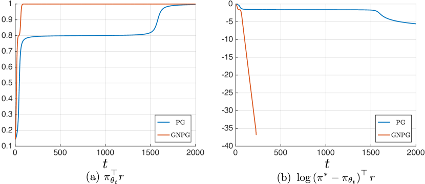
Figure 4: PG and GNPG on $r=(1.0,0.8,0.1)^{\top}$.

We compare PG and GNPG on the one-state MDP problem as shown in Figure 4. Figure 4(a) shows that GNPG escapes from the sub-optimal plateau significantly faster than PG, while Figure 4(b) shows that GNPG follows linear convergence $O(e^{-c\cdot t})$ of sub-optmality, verifying the theoretical results. Similar experimental results on synthetic tree MDPs with multiple states are presented in Appendix F.

6 Generalized Linear Models

Next, we investigate the generalized linear model (GLM) with quasi-maximum likelihood estimate (quasi-MLE), which applied widely in supervised learning. We show that the mean squared error (MSE) of GLM (Hazan et al., 2015) is in the non-convex function class ${\mathcal{Z}}$ in Figure 2, and it satisfies the case (2) in Theorem 1 with $\xi=1/2$. As a result, both GD and GNGD achieve global linear convergence rates $O(e^{-c\cdot t})$, significantly improving the best existing results of $O(1/\sqrt{t})$ (Hazan et al., 2015). We also provide new understandings of using normalization in GLM based on our non-uniform analysis.

6.1 Basic Settings and Notations

Given a training data set ${\mathcal{D}}=\{(x_{i},y_{i})\}_{i\in[N]}$, which consists of $N$ data points, there is a feature map $x_{i}\mapsto\phi(x_{i})\in{\mathbb{R}}^{d}$ for each pair $(x_{i},y_{i})\in{\mathcal{D}}$. We denote $\phi_{i}\coloneqq\phi(x_{i})$ for conciseness. For each data point $x_{i}$, we have $y_{i}\in[0,1]$ as the ground truth likelihood. Following Hazan et al. (2015), our model is parameterized by a weight vector $\theta\in{\mathbb{R}}^{d}$ as ,

$$\pi_{i}=\sigma(\phi_{i}^{\top}\theta)=\frac{1}{1+\exp\{-\phi_{i}^{\top}\theta\}},$$ (14)

where $\sigma:{\mathbb{R}}\to(0,1)$ is the sigmoid activation. The problem is to minimize the mean squared error (MSE),

$$\min_{\theta}{\mathcal{L}}(\theta)=\min_{\theta\in{\mathbb{R}}^{d}}\frac{1}{N}\cdot\sum_{i=1}^{N}{(\pi_{i}-y_{i})^{2}}.$$ (15)

We assume $y_{i}=\pi_{i}^{*}\coloneqq\sigma(\phi_{i}^{\top}\theta^{*})$, where $\theta^{*}\in{\mathbb{R}}^{d}$, and $\left\|\theta^{*}\right\|_{2}<\infty$, which means the target $y_{i}$ is realizable and non-deterministic. According to Hazan et al. (2015), the MSE in Eq. 15 is not quasi-convex (thus not convex). Fortunately, Hazan et al. (2015) manage to show that Eq. 15 satisfies a weaker Strictly-Locally-Quasi-Convex (SLQC) property, based on which they prove the following result:

Theorem 4 (Hazan et al. (2015)).

With diminishing learning rate $\eta_{t}\in\Theta(1/\sqrt{t})$, the normalized gradient descent (NGD) update $\theta_{t+1}\leftarrow\theta_{t}-\eta_{t}\cdot\frac{\partial{\mathcal{L}}(\theta_{t})}{\partial\theta_{t}}\Big{/}\left\|\frac{\partial{\mathcal{L}}(\theta_{t})}{\partial\theta_{t}}\right\|_{2}$ satisfies,

$$\delta(\theta_{t})\coloneqq{\mathcal{L}}(\theta_{t})-{\mathcal{L}}(\theta^{*})\in O(1/\sqrt{t}),$$ (16)

where $\theta^{*}\coloneqq\operatorname*{arg\,min}_{\theta}{{\mathcal{L}}(\theta)}$ is the global optimal solution.

6.2 Fast Convergence using Non-uniform Analysis

Based on the $O(1/\sqrt{t})$ rate for NGD in Theorem 4, Hazan et al. (2015) propose to normalize gradient norm in MSE minimization. However, there is no lower bound for other methods including GD on GLM, and thus it is not clear if there exists a faster rate for GLM optimization.

Surprisingly, we prove that both GD and GNGD actually achieve much faster rates of $O(e^{-c\cdot t})$ using the non-uniform analysis. Our first key finding is to show that the MSE in GLM satisfies a new NŁ inequality with $\xi=1/2$:

Lemma 9 (NŁ).

Denote $u(\theta)\coloneqq\min_{i\in[N]}{\left\{\pi_{i}\cdot\left(1-\pi_{i}\right)\right\}}$, and $v\coloneqq\min_{i\in[N]}{\left\{\pi_{i}^{*}\cdot\left(1-\pi_{i}^{*}\right)\right\}}$. We have,

$$\left\|\frac{\partial{\mathcal{L}}(\theta)}{\partial\theta}\right\|_{2}\geq C(\theta,\phi)\cdot\left[\frac{1}{N}\cdot\sum_{i=1}^{N}{\left(\pi_{i}-\pi_{i}^{*}\right)^{2}}\right]^{\frac{1}{2}},$$ (17)

holds for all $\theta\in{\mathbb{R}}^{d}$, where

$$C(\theta,\phi)=8\cdot u(\theta)\cdot\min\left\{u(\theta),v\right\}\cdot\sqrt{\lambda_{\phi}},$$ (18)

and $\lambda_{\phi}$ is the smallest positive eigenvalue of $\frac{1}{N}\cdot\sum_{i=1}^{N}{\phi_{i}\phi_{i}^{\top}}$.

Remark 7.

It is not clear if results similar to Lemma 9 hold without assuming: (i) realizable optimal prediction $y_{i}=\pi_{i}^{*}\coloneqq\sigma(\phi_{i}^{\top}\theta^{*})$; (ii) non-deterministic optimal prediction $\left\|\theta^{*}\right\|_{2}<\infty$. We leave it as an open question to study non-uniformity of GLM without the above assumptions.

In Lemma 9, $\lambda_{\phi}$ is determined by the feature $\phi$, and $u(\theta)$ shows that the gradient is vanishing when $\pi_{i}$ is near deterministic, which is consistent with the fact that the sigmoid saturates and provides uninformative gradient as the parameter magnitude becomes large.

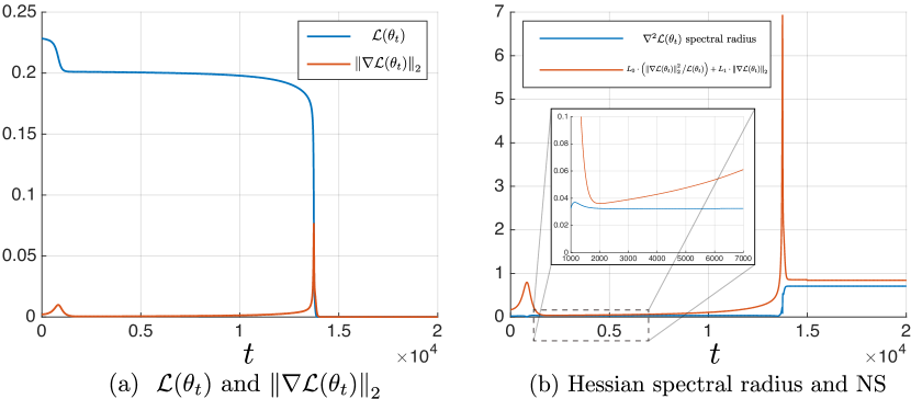
Figure 5: Experiments on GLM using GD.

We run GD on one example with $N=10$ and $d=2$. As shown in Figure 5, the gradient norm $\left\|\nabla{\mathcal{L}}(\theta_{t})\right\|_{2}$ is close to zero at plateaus and near optimum. However, unlike the PG, the spectral radius of the Hessian $\nabla^{2}{\mathcal{L}}(\theta_{t})$ is only close to zero at plateaus, while it approaches positive constant near optimum. This indicates a different NS condition other than Lemmas 2 and 6 is needed, since only gradient norm $\to 0$ cannot upper bound the spectral radius of Hessian $\to c>0$. With some calculations, we prove the following key results:

Lemma 10 (Smoothness and NS).

${\mathcal{L}}(\theta)$ satisfies $\beta$ smoothness with

$$\beta=\frac{3}{8}\cdot\max_{i\in[N]}{\left\|\phi_{i}\right\|_{2}^{2}},$$ (19)

and $\beta(\theta)$ NS with

$$\beta(\theta)=L_{1}\cdot\left\|\frac{\partial{\mathcal{L}}(\theta)}{\partial\theta}\right\|_{2}+L_{0}\cdot\left(\left\|\frac{\partial{\mathcal{L}}(\theta)}{\partial\theta}\right\|_{2}^{2}\Big{/}{\mathcal{L}}(\theta)\right).$$

At the optimal solution $\theta^{*}$, the spectral radius of the Hessian $\frac{\partial^{2}{\mathcal{L}}(\theta^{*})}{\partial(\theta^{*})^{2}}$ is strictly positive. Therefore, the MSE objective of Eq. 15 is in the non-convex function class ${\mathcal{Z}}$ in Figure 2, and it satisfies the case (2) in Theorem 1 with $\xi=1/2$. Combining Lemmas 9 and 10 and applying Theorem 1, we have the following global linear convergence result:

Theorem 5.

With $\eta=1/\beta$, GD update satisfies for all $t\geq 1$, ${\mathcal{L}}(\theta_{t})\leq{\mathcal{L}}(\theta_{1})\cdot e^{-C^{2}\cdot(t-1)}$. With $\eta\in\Theta(1)$, GNGD update satisfies for all $t\geq 1$, ${\mathcal{L}}(\theta_{t})\leq{\mathcal{L}}(\theta_{1})\cdot e^{-C\cdot(t-1)}$, where $C\in(0,1)$, i.e., GNGD is strictly faster than GD.

Theorem 5 significantly improves the $O(1/\sqrt{t})$ rate in Theorem 4. The key difference is that we discovered a new NŁ inequality of Lemma 9 that is satisfied by GLMs. The linear convergence rates are verified in Appendix F.

In Theorem 5, we have $C=\inf_{t\geq 1}{C(\theta_{t},\phi)}$, which is very close to zero if $\pi_{i}$ is near deterministic, and GD suffers sub-optimality plateaus as shown in Figure 1. GNGD has strictly (orders of magnitudes) better constant dependence $C\gg C^{2}$, and escapes plateaus significantly faster than GD. Intuitively, for the GLM in Figure 1, $C$ in Theorem 1 is lower bounded reasonably if $\theta_{1}$ is initialized within some finite distance of the central valley containing $\theta^{*}$.

Combining the NŁ and NS properties (Lemmas 9 and 10), we provide new understandings of using normalization in GLM: (i) First, using standard NGD (Hazan et al., 2015) for all $t\geq 1$ is not a good choice. By examining the asymptotic behaviour as $\theta\to\theta^{*}$, we have $\beta(\theta)\to\beta>0$. However, the normalization $\Big{\|}\frac{\partial{\mathcal{L}}(\theta)}{\partial\theta}\Big{\|}_{2}$ in standard NGD gives incremental updates with adaptive stepsize $\to\infty$. To guarantee convergence, it is necessary to use $\eta_{t}\to 0$, which counteracts normalization and slows down the learning, since it could be not easy to find a learning rate scheme. This is consistent with the $O(e^{-c\cdot t})$ result for GD with $\eta>0$ and without normalization in Theorem 5. (ii) Second, using geometry-aware normalization $\beta(\theta_{t})$ is a better choice than normalizing the gradient norm $\left\|\nabla{\mathcal{L}}(\theta_{t})\right\|_{2}$. We elaborate this point by investigating both the asymptotic and the early-stage behaviours using NS-NŁ. Since $\beta(\theta_{t})\to\beta>0$ asymptotically, GNGD is approaching GD as $\theta_{t}\to\theta^{*}$, which makes GNGD enjoy the same $O(e^{-c\cdot t})$ rate. On the other hand, at early-stage optimization (e.g., close to initialization in Figure 1), when $\theta_{t}$ is far from $\theta^{*}$, we have thus $\beta(\theta_{t})\leq c\cdot\left\|\frac{\partial{\mathcal{L}}(\theta_{t})}{\partial\theta_{t}}\right\|_{2}$. Then GNGD is close to NGD, which guarantees strictly better progresses than GD. This is because of the progress of GNGD in each iteration at this time is about $\left\|\nabla{\mathcal{L}}(\theta_{t})\right\|_{2}$, while the progress of GD is $\left\|\nabla{\mathcal{L}}(\theta_{t})\right\|_{2}^{2}$, and the gradient norm is close to $0$ on plateaus. Using NŁ of Lemma 9, GNGD will have strictly better constant dependence $C$ than $C^{2}$ in GD.

7 Conclusions and Future Work

The main contributions of this paper concern a general characterization and analysis based on non-uniform properties, which are not only sufficiently general to cover concrete examples, but also significantly improve convergence rates over previous work and even over classical lower bounds. The most exciting part is the techniques apply to important applications in machine learning that involve non-convex optimization problems. One direction is to further push the analysis to other domains with more complex function approximators, including neural networks (Allen-Zhu et al., 2019). Another valuable future work is to incorporate stochastic gradient (Karimi et al., 2016) and other adaptive gradient-based methods (Kingma & Ba, 2014) in the analysis. Finally, applying other cases of non-uniform properties beyond those mentioned in this paper would be interesting.

Appendix

The appendix is organized as follows.

• Appendix A: proofs for general optimization results in Section 4.

  • Section A.1: proofs for the main Theorem 1.

  • Section A.2: proofs for the function classes, i.e., Propositions 1, 2, 3 and 4.

• Appendix B: proofs for policy gradient in Section 5.

  • Section B.1: proofs for one-state MDPs.

  • Section B.2: proofs for general MDPs.

• Appendix C: proofs for generalized linear model in Section 6.

• Appendix D: miscellaneous extra supporting results those are not mentioned in the main paper.

• Appendix E: non-convex (non-concave) examples for the NŁ inequality in literature.

• Appendix F: additional simulation results which are not in the main paper.

Appendix A Proofs for Section 4

A.1 Main Theorem 1

Theorem 1. Suppose $f:\Theta\to{\mathbb{R}}$ satisfies NS with $\beta(\theta)$ and the NŁ inequality with $(C(\theta),\xi)$. Suppose $C\coloneqq\inf_{t\geq 1}{C(\theta_{t})}>0$ for GD and GNGD. Let $\delta(\theta)\coloneqq f(\theta)-f(\theta^{*})$ be the sub-optimality gap. The following hold:

(1a)

if $\beta(\theta)\leq c\cdot\delta(\theta)^{1-2\xi}$ with $\xi\in(-\infty,1/2)$, then the conclusions of (1b) hold;

(1b)

if $\beta(\theta)\leq c\cdot\left\|\nabla f(\theta)\right\|_{2}^{\frac{1-2\xi}{1-\xi}}$ with $\xi\in(-\infty,1/2)$, then GD with $\eta\in O(1)$ achieves $\delta(\theta_{t})\in\Theta(1/t^{\frac{1}{1-2\xi}})$, and GNGD achieves $\delta(\theta_{t})\in O(e^{-t})$.

(2a)

if $\beta(\theta)\leq L_{0}+L_{1}\cdot\left\|\nabla f(\theta)\right\|_{2}$, then the conclusions of (2b) hold;

(2b)

if $\beta(\theta)\leq L_{0}\cdot\frac{\left\|\nabla f(\theta)\right\|^{2}}{\delta(\theta)^{2-2\xi}}+L_{1}\cdot\left\|\nabla f(\theta)\right\|_{2}$, then GD and GNGD both achieve $\delta(\theta_{t})\in O(1/t^{\frac{1}{1-2\xi}})$ when $\xi\in(-\infty,1/2)$, and $O(e^{-t})$ when $\xi=1/2$. GNGD has strictly better constant than GD ($1\geq C\geq C^{2}$).

(3a)

if $\beta(\theta)\!\leq\!c\!\cdot\!\left\|\nabla f(\theta)\right\|_{2}^{\frac{1-2\xi}{1-\xi}}\!$ with $\xi\in(1/2,1)$, then the conclusions of (3b) hold;

(3b)

if $\beta(\theta)\leq c\cdot\delta(\theta)^{1-2\xi}$ with $\xi\in(1/2,1)$, then GD with $\eta\in\Theta(1)$ does not converge, while GNGD achieves $\delta(\theta_{t})\in O(e^{-t})$.

Proof.

(1a) First part: $O(1/t^{\frac{1}{1-2\xi}})$ upper bound for GD update $\theta_{t+1}\leftarrow\theta_{t}-\eta\cdot\nabla f(\theta_{t})$ with $\eta\in O(1)$.

We show that using GD with learning rate $\eta=\frac{1}{c\cdot\delta(\theta_{1})^{1-2\xi}}$, the sub-optimality $\delta(\theta_{t})$ is monotonically decreasing. And thus there exists a universal constant $\beta>0$ such that $\beta(\theta_{t})\leq\beta$, for all $t\geq 1$.

Denote $\beta\coloneqq c\cdot\delta(\theta_{1})^{1-2\xi}$. We have $\beta\in(0,\infty)$, since $f(\theta^{*})>-\infty$, and $f(\theta^{*})<f(\theta_{1})<\infty$. By assumption, we have $\beta(\theta_{1})\leq\beta$. According to Lemma 11, using GD with $\eta=\frac{1}{\beta}$, we have,

$$\delta(\theta_{2})-\delta(\theta_{1})=f(\theta_{2})-f(\theta_{1})\leq 0.$$ (20)

Therefore, we have,

$$\beta(\theta_{2}) \leq c\cdot\delta(\theta_{2})^{1-2\xi}\qquad\left(\text{by assumption}\right)$$ (21)

$$\leq c\cdot\delta(\theta_{1})^{1-2\xi}\qquad\left(0<\delta(\theta_{2})\leq\delta(\theta_{1})\text{ and }\xi<1/2\right)$$ (22)

$$=\beta.$$ (23)

Repeating similar arguments of Eqs. 20 and 21, we have, for all $t\geq 1$, $\beta(\theta_{t})\leq\beta$ and,

$$0<\delta(\theta_{t+1})\leq\delta(\theta_{t}).$$ (24)

Therefore, we have, for all $t\geq 1$ (or using Lemma 11),

$$\delta(\theta_{t+1})-\delta(\theta_{t}) =f(\theta_{t+1})-f(\theta_{t})$$ (25)

$$\leq\nabla f(\theta_{t})^{\top}\left(\theta_{t+1}-\theta_{t}\right)+\frac{\beta(\theta_{t})}{2}\cdot\left\|\theta_{t+1}-\theta_{t}\right\|_{2}^{2}\qquad\left(\text{NS}\right)$$ (26)

$$\leq\nabla f(\theta_{t})^{\top}\left(\theta_{t+1}-\theta_{t}\right)+\frac{\beta}{2}\cdot\left\|\theta_{t+1}-\theta_{t}\right\|_{2}^{2}\qquad\left(\beta(\theta_{t})\leq\beta\right)$$ (27)

$$=-\frac{1}{2\beta}\cdot\left\|\nabla f(\theta_{t})\right\|_{2}^{2}\qquad\left(\theta_{t+1}\leftarrow\theta_{t}-\frac{1}{\beta}\cdot\nabla f(\theta_{t})\right)$$ (28)

$$\leq-\frac{1}{2\beta}\cdot C(\theta_{t})^{2}\cdot\delta(\theta_{t})^{2-2\xi}\qquad\left(\text{N\L{}}\right)$$ (29)

$$\leq-\frac{1}{2\beta}\cdot C^{2}\cdot\delta(\theta_{t})^{2-2\xi}.\qquad\left(C\coloneqq\inf_{t\geq 1}{C(\theta_{t})}>0\right)$$ (30)

According to Lemma 13, given any $\alpha>0$, we have, for all $x\in[0,1]$,

$$\frac{1}{\alpha}\cdot(1-x^{\alpha})\geq x^{\alpha}\cdot\left(1-x\right).$$ (31)

Let $\alpha=1-2\xi>0$, since $\xi<1/2$. Also let $x=\frac{\delta(\theta_{t+1})}{\delta(\theta_{t})}\in(0,1]$ due to Eq. 24. We have,

$$\frac{1}{1-2\xi}\cdot\left[1-\frac{\delta(\theta_{t+1})^{1-2\xi}}{\delta(\theta_{t})^{1-2\xi}}\right]\geq\frac{\delta(\theta_{t+1})^{1-2\xi}}{\delta(\theta_{t})^{1-2\xi}}\cdot\left[1-\frac{\delta(\theta_{t+1})}{\delta(\theta_{t})}\right].$$ (32)

Next, we have,

$$\frac{1}{\delta(\theta_{t})^{1-2\xi}} =\frac{1}{\delta(\theta_{1})^{1-2\xi}}+\frac{1}{\delta(\theta_{t})^{1-2\xi}}-\frac{1}{\delta(\theta_{1})^{1-2\xi}}$$ (33)

$$=\frac{1}{\delta(\theta_{1})^{1-2\xi}}+\sum_{s=1}^{t-1}{\left[\frac{1}{\delta(\theta_{s+1})^{1-2\xi}}-\frac{1}{\delta(\theta_{s})^{1-2\xi}}\right]}$$ (34)

$$=\frac{1}{\delta(\theta_{1})^{1-2\xi}}+\sum_{s=1}^{t-1}{\frac{1-2\xi}{\delta(\theta_{s+1})^{1-2\xi}}\cdot\frac{1}{1-2\xi}\cdot\left[1-\frac{\delta(\theta_{s+1})^{1-2\xi}}{\delta(\theta_{s})^{1-2\xi}}\right]}$$ (35)

$$\geq\frac{1}{\delta(\theta_{1})^{1-2\xi}}+\sum_{s=1}^{t-1}{\frac{1-2\xi}{\bcancel{\delta(\theta_{s+1})^{1-2\xi}}}\cdot\frac{\bcancel{\delta(\theta_{s+1})^{1-2\xi}}}{\delta(\theta_{s})^{1-2\xi}}\cdot\left[1-\frac{\delta(\theta_{s+1})}{\delta(\theta_{s})}\right]}\qquad\left(\text{by \lx@cref{creftype~refnum}{eq:general_optimization_main_result_1_1a_intermediate_2}}\right)$$ (36)

$$=\frac{1}{\delta(\theta_{1})^{1-2\xi}}+\sum_{s=1}^{t-1}{\frac{1-2\xi}{\delta(\theta_{s})^{2-2\xi}}\cdot\left[\delta(\theta_{s})-\delta(\theta_{s+1})\right]}$$ (37)

$$\geq\frac{1}{\delta(\theta_{1})^{1-2\xi}}+\sum_{s=1}^{t-1}{\frac{1-2\xi}{\bcancel{\delta(\theta_{s})^{2-2\xi}}}\cdot\frac{C^{2}}{2\beta}\cdot\bcancel{\delta(\theta_{s})^{2-2\xi}}}\qquad\left(\text{by \lx@cref{creftype~refnum}{eq:general_optimization_main_result_1_1a_intermediate_1}}\right)$$ (38)

$$=\frac{1}{\delta(\theta_{1})^{1-2\xi}}+\frac{(1-2\xi)\cdot C^{2}}{2\beta}\cdot(t-1),$$ (39)

which implies for all $t\geq 1$,

$$f(\theta_{t})-f(\theta^{*})=\delta(\theta_{t})\leq\left[\frac{1}{\left(f(\theta_{1})-f(\theta^{*})\right)^{1-2\xi}}+\frac{(1-2\xi)\cdot C^{2}}{2\beta}\cdot(t-1)\right]^{-\frac{1}{1-2\xi}}\in O\left(\frac{1}{t^{\frac{1}{1-2\xi}}}\right).$$ (40)

(1a) Second part:

$\Omega(1/t^{\frac{1}{1-2\xi}})$ lower bound for GD update $\theta_{t+1}\leftarrow\theta_{t}-\eta_{t}\cdot\nabla f(\theta_{t})$ with $\eta_{t}\in(0,1]$.

According to the NS property of Definition 3, we have, for all $\theta$ and $\theta^{\prime}$,

$$f(\theta^{\prime})\leq f(\theta)+\nabla f(\theta)^{\top}\left(\theta^{\prime}-\theta\right)+\frac{\beta(\theta)}{2}\cdot\left\|\theta^{\prime}-\theta\right\|_{2}^{2}.$$ (41)

Fix $\theta$ and take minimum over $\theta^{\prime}$ on both sides of the above inequality. Then we have,

$$f(\theta^{*}) \leq f(\theta)+\min_{\theta^{\prime}}\left\{\nabla f(\theta)^{\top}\left(\theta^{\prime}-\theta\right)+\frac{\beta(\theta)}{2}\cdot\left\|\theta^{\prime}-\theta\right\|_{2}^{2}\right\}$$ (42)

$$=f(\theta)-\frac{1}{\beta(\theta)}\cdot\left\|\nabla f(\theta)\right\|_{2}^{2}+\frac{1}{2\cdot\beta(\theta)}\cdot\left\|\nabla f(\theta)\right\|_{2}^{2}\qquad\left(\theta^{\prime}=\theta-\frac{1}{\beta(\theta)}\cdot\nabla f(\theta)\right)$$ (43)

$$=f(\theta)-\frac{1}{2\cdot\beta(\theta)}\cdot\left\|\nabla f(\theta)\right\|_{2}^{2},$$ (44)

which implies,

$$\left\|\nabla f(\theta)\right\|_{2}^{2} \leq 2\cdot\beta(\theta)\cdot\delta(\theta)$$ (45)

$$\leq 2\cdot c\cdot\delta(\theta)^{2-2\xi}.\qquad\left(\beta(\theta)\leq c\cdot\delta(\theta)^{1-2\xi}\right)$$ (46)

Therefore, we have,

$$\delta(\theta_{t})-\delta(\theta_{t+1}) =f(\theta_{t})-f(\theta_{t+1})+\nabla f(\theta_{t})^{\top}\left(\theta_{t+1}-\theta_{t}\right)-\nabla f(\theta_{t})^{\top}\left(\theta_{t+1}-\theta_{t}\right)$$ (47)

$$\leq\frac{\beta}{2}\cdot\left\|\theta_{t+1}-\theta_{t}\right\|_{2}^{2}-\nabla f(\theta_{t})^{\top}\left(\theta_{t+1}-\theta_{t}\right)\qquad\left(\text{by NS and }\beta(\theta_{t})\leq\beta\right)$$ (48)

$$=\left(\frac{\beta}{2}\cdot\eta_{t}^{2}+\eta_{t}\right)\cdot\left\|\nabla f(\theta_{t})\right\|_{2}^{2}\qquad\left(\theta_{t+1}\leftarrow\theta_{t}-\eta_{t}\cdot\nabla f(\theta_{t})\right)$$ (49)

$$\leq\left(\frac{\beta}{2}\cdot\eta_{t}^{2}+\eta_{t}\right)\cdot 2\cdot c\cdot\delta(\theta_{t})^{2-2\xi}\qquad\left(\text{by \lx@cref{creftype~refnum}{eq:general_optimization_main_result_1_1a_intermediate_3}}\right)$$ (50)

$$\leq\left(\beta+2\right)\cdot c\cdot\delta(\theta_{t})^{2-2\xi}.\qquad\left(\eta_{t}\in(0,1]\right)$$ (51)

Next, we show that $\frac{\delta(\theta_{t+1})}{\delta(\theta_{t})}\geq\frac{3-4\xi}{4-4\xi}$ holds for all large enough $t\geq 1$ by contradiction. According to the upper bound results in the first part, we have $\delta(\theta_{t})\to 0$ as $t\to\infty$. Suppose $\frac{\delta(\theta_{t+1})}{\delta(\theta_{t})}<\frac{3-4\xi}{4-4\xi}$, where $t\geq 1$ is large enough and $\delta(\theta_{t})$ is small enough. We have,

$$\delta(\theta_{t+1}) \geq\delta(\theta_{t})-\left(\beta+2\right)\cdot c\cdot\delta(\theta_{t})^{2-2\xi}\qquad\left(\text{by \lx@cref{creftype~refnum}{eq:general_optimization_main_result_1_1a_intermediate_4}}\right)$$ (52)

$$>\frac{4-4\xi}{3-4\xi}\cdot\delta(\theta_{t+1})-\left(\beta+2\right)\cdot c\cdot\left(\frac{4-4\xi}{3-4\xi}\right)^{2-2\xi}\cdot\delta(\theta_{t+1})^{2-2\xi},$$ (53)

where the last inequality is because of the function $f:x\mapsto x-a\cdot x^{2-2\xi}$ with $a>0$ is monotonically increasing for all $0<x\leq\frac{1}{\left[(2-2\xi)a\right]^{1/(1-2\xi)}}$. Eq. 52 implies that,

$$\delta(\theta_{t+1})^{1-2\xi}>\frac{1}{3-4\xi}\cdot\frac{1}{(\beta+2)\cdot c}\cdot\left(\frac{3-4\xi}{4-4\xi}\right)^{2-2\xi},$$ (54)

for large enough $t\geq 1$, which is a contradiction with $\delta(\theta_{t})\to 0$ as $t\to\infty$. Thus we have $\frac{\delta(\theta_{t+1})}{\delta(\theta_{t})}\geq\frac{3-4\xi}{4-4\xi}$ holds for all large enough $t\geq 1$. Denote

$$t_{0}\coloneqq\min\Big{\{}t\geq 1:\frac{\delta(\theta_{s+1})}{\delta(\theta_{s})}\geq\frac{3-4\xi}{4-4\xi},\text{ for all }s\geq t\Big{\}}.$$ (55)

According to Lemma 14, given any $\alpha>0$, we have, for all $x\in\left[\frac{2\alpha+1}{2\alpha+2},1\right]$,

$$\frac{1}{2\alpha}\cdot(1-x^{\alpha})\leq x^{\alpha}\cdot\left(1-x\right).$$ (56)

Let $\alpha=1-2\xi>0$, since $\xi<1/2$. We have $\frac{2\alpha+1}{2\alpha+2}=\frac{3-4\xi}{4-4\xi}$. Also let $x=\frac{\delta(\theta_{t+1})}{\delta(\theta_{t})}\in\left[\frac{3-4\xi}{4-4\xi},1\right]$. We have,

$$\frac{1}{2\cdot(1-2\xi)}\cdot\left[1-\frac{\delta(\theta_{t+1})^{1-2\xi}}{\delta(\theta_{t})^{1-2\xi}}\right]\leq\frac{\delta(\theta_{t+1})^{1-2\xi}}{\delta(\theta_{t})^{1-2\xi}}\cdot\left[1-\frac{\delta(\theta_{t+1})}{\delta(\theta_{t})}\right],$$ (57)

for all $t\geq t_{0}$. On the other hand, since $t_{0}\in O(1)$ and $1-2\xi>0$, we have, for all $t<t_{0}$,

$$\delta(\theta_{t+1})^{1-2\xi}\geq c_{0}>0.$$ (58)

Next, we have, for all $t\geq t_{0}$,

$$\frac{1}{\delta(\theta_{t})^{1-2\xi}}=\frac{1}{\delta(\theta_{1})^{1-2\xi}}+\sum_{s=1}^{t-1}{\left[\frac{1}{\delta(\theta_{s+1})^{1-2\xi}}-\frac{1}{\delta(\theta_{s})^{1-2\xi}}\right]}$$ (59)

$$=\frac{1}{\delta(\theta_{1})^{1-2\xi}}+\sum_{s=1}^{t_{0}-1}{\frac{1}{\delta(\theta_{s+1})^{1-2\xi}}\cdot\left[1-\frac{\delta(\theta_{s+1})^{1-2\xi}}{\delta(\theta_{s})^{1-2\xi}}\right]}+\sum_{s=t_{0}}^{t-1}{\frac{2\cdot(1-2\xi)}{\delta(\theta_{s+1})^{1-2\xi}}\cdot\frac{1}{2\cdot(1-2\xi)}\cdot\left[1-\frac{\delta(\theta_{s+1})^{1-2\xi}}{\delta(\theta_{s})^{1-2\xi}}\right]}$$ (60)

$$\leq\frac{1}{\delta(\theta_{1})^{1-2\xi}}+\sum_{s=1}^{t_{0}-1}{\frac{1}{c_{0}}\cdot 1}+\sum_{s=t_{0}}^{t-1}{\frac{2\cdot(1-2\xi)}{\bcancel{\delta(\theta_{s+1})^{1-2\xi}}}\cdot\frac{\bcancel{\delta(\theta_{s+1})^{1-2\xi}}}{\delta(\theta_{s})^{1-2\xi}}\cdot\left[1-\frac{\delta(\theta_{s+1})}{\delta(\theta_{s})}\right]}\qquad\left(\text{by \lx@cref{creftype~refnum}{eq:general_optimization_main_result_1_1a_intermediate_6}}\right)$$ (61)

$$=\frac{1}{\delta(\theta_{1})^{1-2\xi}}+\frac{t_{0}-1}{c_{0}}+\sum_{s=t_{0}}^{t-1}{\frac{2\cdot(1-2\xi)}{\delta(\theta_{s})^{2-2\xi}}\cdot\left[\delta(\theta_{s})-\delta(\theta_{s+1})\right]}$$ (62)

$$\leq\frac{1}{\delta(\theta_{1})^{1-2\xi}}+\frac{t_{0}-1}{c_{0}}+\sum_{s=t_{0}}^{t-1}{\frac{2\cdot(1-2\xi)}{\bcancel{\delta(\theta_{s})^{2-2\xi}}}\cdot\left(\beta+2\right)\cdot c\cdot\bcancel{\delta(\theta_{s})^{2-2\xi}}}\qquad\left(\text{by \lx@cref{creftype~refnum}{eq:general_optimization_main_result_1_1a_intermediate_4}}\right)$$ (63)

$$=\frac{1}{\delta(\theta_{1})^{1-2\xi}}+\frac{t_{0}-1}{c_{0}}+2\cdot(1-2\xi)\cdot\left(\beta+2\right)\cdot c\cdot(t-t_{0}),$$ (64)

which implies for all large enough $t\geq 1$,

$$f(\theta_{t})-f(\theta^{*})=\delta(\theta_{t})\geq\left[\frac{1}{\left(f(\theta_{1})-f(\theta^{*})\right)^{1-2\xi}}+\frac{t_{0}-1}{c_{0}}+2\cdot(1-2\xi)\cdot\left(\beta+2\right)\cdot c\cdot(t-t_{0})\right]^{-\frac{1}{1-2\xi}}\in\Omega\left(\frac{1}{t^{\frac{1}{1-2\xi}}}\right).$$ (65)

(1a) Third part:

$O(e^{-t})$ upper bound for GNGD update $\theta_{t+1}\leftarrow\theta_{t}-\frac{\nabla f(\theta_{t})}{\beta(\theta_{t})}$.

We have, for all $t\geq 1$ (or using Lemma 12),

$$\delta(\theta_{t+1})-\delta(\theta_{t}) =f(\theta_{t+1})-f(\theta_{t})$$ (66)

$$\leq\nabla f(\theta_{t})^{\top}\left(\theta_{t+1}-\theta_{t}\right)+\frac{\beta(\theta_{t})}{2}\cdot\left\|\theta_{t+1}-\theta_{t}\right\|_{2}^{2}\qquad\left(\text{NS}\right)$$ (67)

$$=-\frac{1}{\beta(\theta_{t})}\cdot\left\|\nabla f(\theta_{t})\right\|_{2}^{2}+\frac{1}{2}\cdot\frac{1}{\beta(\theta_{t})}\cdot\left\|\nabla f(\theta_{t})\right\|_{2}^{2}\qquad\left(\theta_{t+1}\leftarrow\theta_{t}-\frac{\nabla f(\theta_{t})}{\beta(\theta_{t})}\right)$$ (68)

$$=-\frac{1}{2\cdot\beta(\theta_{t})}\cdot\left\|\nabla f(\theta_{t})\right\|_{2}^{2}$$ (69)

$$\leq-\frac{1}{2\cdot\beta(\theta_{t})}\cdot C(\theta_{t})^{2}\cdot\delta(\theta_{t})^{2-2\xi}\qquad\left(\text{N\L{}}\right)$$ (70)

$$\leq-\frac{1}{2\cdot\beta(\theta_{t})}\cdot C^{2}\cdot\delta(\theta_{t})^{2-2\xi}\qquad\left(C\coloneqq\inf_{t\geq 1}{C(\theta_{t})}>0\right)$$ (71)

$$\leq-\frac{C^{2}}{2\cdot c}\cdot\delta(\theta_{t}),\qquad\left(\beta(\theta_{t})\leq c\cdot\delta(\theta_{t})^{1-2\xi}\right)$$ (72)

which implies for all $t\geq 1$,

$$f(\theta_{t})-f(\theta^{*})=\delta(\theta_{t}) \leq\left(1-C^{2}/(2\cdot c)\right)\cdot\delta(\theta_{t-1})$$ (73)

$$\leq\exp\left\{-C^{2}/(2\cdot c)\right\}\cdot\delta(\theta_{t-1})$$ (74)

$$\leq\exp\left\{-(t-1)\cdot C^{2}/(2\cdot c)\right\}\cdot\delta(\theta_{1})$$ (75)

$$=\exp\left\{-(t-1)\cdot C^{2}/(2\cdot c)\right\}\cdot\left(f(\theta_{1})-f(\theta^{*})\right).$$ (76)

(1b) First part:

$O(1/t^{\frac{1}{1-2\xi}})$ upper bound for GD update $\theta_{t+1}\leftarrow\theta_{t}-\eta\cdot\nabla f(\theta_{t})$ with $\eta\in O(1)$.

Denote $\beta_{1}\coloneqq c\cdot\left\|\nabla f(\theta_{1})\right\|_{2}^{\frac{1-2\xi}{1-\xi}}$. We have $\beta_{1}\in(0,\infty)$, since $f$ is differentiable (Definition 3). Using $\eta\leq\frac{1}{\beta_{1}}$ and according to Lemma 11, we have $\delta(\theta_{2})\leq\delta(\theta_{1})$. Denote $\beta_{2}\coloneqq c\cdot\left\|\nabla f(\theta_{2})\right\|_{2}^{\frac{1-2\xi}{1-\xi}}$. We also have $\beta_{2}\in(0,\infty)$. Repeating the update, we generate $\left\{\theta_{t}\right\}_{t\geq 1}$ such that $\delta(\theta_{t+1})\leq\delta(\theta_{t})$. Denote

$$\beta\coloneqq\sup_{t\geq 1}{\left\{\beta_{t}\right\}}=\sup_{t\geq 1}{\left\{c\cdot\left\|\nabla f(\theta_{2})\right\|_{2}^{\frac{1-2\xi}{1-\xi}}\right\}}.$$ (77)

Now we have $0\leq\delta(\theta_{t+1})\leq\delta(\theta_{t})\leq\cdots\leq\delta(\theta_{1})$. According to the monotone convergence theorem, $\delta(\theta_{t})$ converges to some finite value. And the gradient $\left\|\nabla f(\theta_{t})\right\|_{2}\to 0$, otherwise a small gradient update can decrease the sub-optimality, which is a contradiction with convergence. Thus we have $\beta\in(\beta_{1},\infty)$, since $\beta_{t}\to 0$ as $t\to\infty$. Using $\eta=\frac{1}{\beta}$, we have $\eta\leq\frac{1}{\beta_{t}}$ holds for all $t\geq 1$, and,

$$\beta(\theta_{t})\leq c\cdot\left\|\nabla f(\theta_{t})\right\|_{2}^{\frac{1-2\xi}{1-\xi}}=\beta_{t}\leq\beta.$$ (78)

Using similar calculations in the first part of (1a), we have the $O(1/t^{\frac{1}{1-2\xi}})$ upper bound.

(1b) Second part:

$\Omega(1/t^{\frac{1}{1-2\xi}})$ lower bound for GD update $\theta_{t+1}\leftarrow\theta_{t}-\eta_{t}\cdot\nabla f(\theta_{t})$ with $\eta_{t}\in(0,1]$.

According to Eq. 45, we have,

$$\left\|\nabla f(\theta)\right\|_{2}^{2} \leq 2\cdot\beta(\theta)\cdot\delta(\theta)$$ (79)

$$\leq 2\cdot c\cdot\left\|\nabla f(\theta)\right\|_{2}^{\frac{1-2\xi}{1-\xi}}\cdot\delta(\theta),\qquad\left(\beta(\theta)\leq c\cdot\left\|\nabla f(\theta)\right\|_{2}^{\frac{1-2\xi}{1-\xi}}\right)$$ (80)

which is equivalent to,

$$\left\|\nabla f(\theta)\right\|_{2}^{2}\leq 2\cdot c_{1}\cdot\delta(\theta)^{2-2\xi},$$ (81)

where $c_{1}\coloneqq\frac{1}{2}\cdot\left(2\cdot c\right)^{2-2\xi}$. According to Eq. 47, we have,

$$\delta(\theta_{t})-\delta(\theta_{t+1}) \leq\left(\frac{\beta}{2}\cdot\eta_{t}^{2}+\eta_{t}\right)\cdot\left\|\nabla f(\theta_{t})\right\|_{2}^{2}$$ (82)

$$\leq\left(\beta+2\right)\cdot c_{1}\cdot\delta(\theta_{t})^{2-2\xi}.\qquad\left(\text{by \lx@cref{creftype~refnum}{eq:general_optimization_main_result_1_1b_intermediate_2} and }\eta_{t}\in(0,1]\right)$$ (83)

Using similar calculations in the second part of (1a), we have the $\Omega(1/t^{\frac{1}{1-2\xi}})$ lower bound.

(1b) Third part:

$O(e^{-t})$ upper bound for GNGD update $\theta_{t+1}\leftarrow\theta_{t}-\frac{\nabla f(\theta_{t})}{\beta(\theta_{t})}$.

According to Lemma 12, we have, for all $t\geq 1$,

$$\delta(\theta_{t+1})-\delta(\theta_{t}) \leq-\frac{1}{2\cdot\beta(\theta_{t})}\cdot\left\|\nabla f(\theta_{t})\right\|_{2}^{2}$$ (84)

$$\leq-\frac{1}{2\cdot c}\cdot\left\|\nabla f(\theta_{t})\right\|_{2}^{\frac{1}{1-\xi}}\qquad\left(\beta(\theta_{t})\leq c\cdot\left\|\nabla f(\theta_{t})\right\|_{2}^{\frac{1-2\xi}{1-\xi}}\right)$$ (85)

$$\leq-\frac{1}{2\cdot c}\cdot C(\theta_{t})^{\frac{1}{1-\xi}}\cdot\delta(\theta_{t})\qquad\left(\text{N\L{}}\right)$$ (86)

$$\leq-\frac{1}{2\cdot c}\cdot C^{\frac{1}{1-\xi}}\cdot\delta(\theta_{t}),\qquad\left(C\coloneqq\inf_{t\geq 1}{C(\theta_{t})}>0\right)$$ (87)

which implies (similar to Eq. 73),

$$f(\theta_{t})-f(\theta^{*})=\delta(\theta_{t})\leq\exp\left\{-(t-1)\cdot C^{\frac{1}{1-\xi}}/(2\cdot c)\right\}\cdot\left(f(\theta_{1})-f(\theta^{*})\right).$$ (88)

(2a) First part:

$O(1/t^{\frac{1}{1-2\xi}})$ upper bound for GD when $\xi<1/2$.

Similar to the first part of (1b), we denote $\beta_{t}\coloneqq L_{0}+L_{1}\cdot\left\|\nabla f(\theta_{t})\right\|_{2}$ and $\beta\coloneqq\sup_{t\geq 1}{\left\{\beta_{t}\right\}}\in(L_{0},\infty)$ since $\left\|\nabla f(\theta_{t})\right\|_{2}\to 0$ as $t\to\infty$. Using $\eta=\frac{1}{\beta}$, we have $\eta\leq\frac{1}{\beta_{t}}$ holds for all $t\geq 1$ and $\beta(\theta_{t})\leq L_{0}+L_{1}\cdot\left\|\nabla f(\theta_{t})\right\|_{2}\leq\beta$. According to Eq. 25 and the first part of (1a), we have the $O(1/t^{\frac{1}{1-2\xi}})$ upper bound.

(2a) Second part:

$O(e^{-t})$ upper bound for GD when $\xi=1/2$.

According to Lemma 11, we have, for all $t\geq 1$,

$$\delta(\theta_{t+1})-\delta(\theta_{t}) \leq-\frac{1}{2\beta}\cdot\left\|\nabla f(\theta_{t})\right\|_{2}^{2}$$ (89)

$$\leq-\frac{1}{2\beta}\cdot C(\theta_{t})^{2}\cdot\delta(\theta_{t})\qquad\left(\text{N\L{} with }\xi=1/2\right)$$ (90)

$$\leq-\frac{1}{2\beta}\cdot C^{2}\cdot\delta(\theta_{t}),\qquad\left(C\coloneqq\inf_{t\geq 1}{C(\theta_{t})}>0\right)$$ (91)

which implies (similar to Eq. 73),

$$f(\theta_{t})-f(\theta^{*})=\delta(\theta_{t})\leq\exp\left\{-(t-1)\cdot C^{2}/(2\beta)\right\}\cdot\left(f(\theta_{1})-f(\theta^{*})\right).$$ (92)

(2a) Third part:

$O(1/t^{\frac{1}{1-2\xi}})$ upper bound for GNGD when $\xi<1/2$.

According to Lemma 12, we have, for all $t\geq 1$,

$$\delta(\theta_{t+1})-\delta(\theta_{t}) \leq-\frac{1}{2\cdot\beta(\theta_{t})}\cdot\left\|\nabla f(\theta_{t})\right\|_{2}^{2}$$ (93)

$$\leq-\frac{1}{2}\cdot\frac{\left\|\nabla f(\theta_{t})\right\|_{2}^{2}}{L_{0}+L_{1}\cdot\left\|\nabla f(\theta_{t})\right\|_{2}}\qquad\left(\beta(\theta_{t})\leq L_{0}+L_{1}\cdot\left\|\nabla f(\theta_{t})\right\|_{2}\right)$$ (94)

$$\leq-\frac{1}{2}\cdot\frac{\left\|\nabla f(\theta_{t})\right\|_{2}^{2}}{L_{0}+L_{1}\cdot\beta}\qquad\left(\beta\coloneqq\sup_{t\geq 1}{\left\{\left\|\nabla f(\theta_{t})\right\|_{2}\right\}}\in(\left\|\nabla f(\theta_{1})\right\|_{2},\infty)\right)$$ (95)

$$\leq-\frac{1}{2}\cdot\frac{C^{2}}{L_{0}+L_{1}\cdot\beta}\cdot\delta(\theta_{t})^{2-2\xi},\qquad\left(\text{N\L{} and }C\coloneqq\inf_{t\geq 1}{C(\theta_{t})}>0\right)$$ (96)

which is similar to Eq. 25. Using similar calculations in the first part of (1a), we have the $O(1/t^{\frac{1}{1-2\xi}})$ upper bound.

(2a) Fourth part:

$O(e^{-t})$ upper bound for GNGD when $\xi=1/2$.

We have, for all $t\geq 1$,

$$\delta(\theta_{t+1})-\delta(\theta_{t}) \leq-\frac{1}{2}\cdot\frac{\left\|\nabla f(\theta_{t})\right\|_{2}^{2}}{L_{0}+L_{1}\cdot\beta}\qquad\left(\text{by \lx@cref{creftype~refnum}{eq:general_optimization_main_result_1_2a_intermediate_1}}\right)$$ (97)

$$\leq-\frac{1}{2}\cdot\frac{C^{2}}{L_{0}+L_{1}\cdot\beta}\cdot\delta(\theta_{t}),\qquad\left(\text{N\L{} with }\xi=1/2\text{ and }C\coloneqq\inf_{t\geq 1}{C(\theta_{t})}>0\right)$$ (98)

which implies (similar to Eq. 73),

$$f(\theta_{t})-f(\theta^{*})=\delta(\theta_{t})\leq\exp\left\{-(t-1)\cdot C^{2}/(2\cdot(L_{0}+L_{1}\cdot\beta))\right\}\cdot\left(f(\theta_{1})-f(\theta^{*})\right).$$ (99)

(2b) First part:

$O(1/t^{\frac{1}{1-2\xi}})$ upper bound for GD when $\xi<1/2$.

Denote $\beta_{t}\coloneqq L_{0}\cdot\frac{\left\|\nabla f(\theta_{t})\right\|^{2}}{\delta(\theta_{t})^{2-2\xi}}+L_{1}\cdot\left\|\nabla f(\theta_{t})\right\|_{2}$ and $\beta\coloneqq\sup_{t\geq 1}{\left\{\beta_{t}\right\}}\in(\beta_{1},\infty)$. According to Eq. 25 and the first part of (1a), we have the $O(1/t^{\frac{1}{1-2\xi}})$ upper bound.

(2b) Second part:

$O(e^{-t})$ upper bound for GD when $\xi=1/2$.

According to Lemma 11, we have, for all $t\geq 1$ (same as the second part of (2a)),

$$\delta(\theta_{t+1})-\delta(\theta_{t}) \leq-\frac{1}{2\beta}\cdot\left\|\nabla f(\theta_{t})\right\|_{2}^{2}$$ (100)

$$\leq-\frac{1}{2\beta}\cdot C(\theta_{t})^{2}\cdot\delta(\theta_{t})\qquad\left(\text{N\L{} with }\xi=1/2\right)$$ (101)

$$\leq-\frac{1}{2\beta}\cdot C^{2}\cdot\delta(\theta_{t}),\qquad\left(C\coloneqq\inf_{t\geq 1}{C(\theta_{t})}>0\right)$$ (102)

which implies (similar to Eq. 73),

$$f(\theta_{t})-f(\theta^{*})=\delta(\theta_{t})\leq\exp\left\{-(t-1)\cdot C^{2}/(2\beta)\right\}\cdot\left(f(\theta_{1})-f(\theta^{*})\right).$$ (103)

(2b) Third part:

$O(1/t^{\frac{1}{1-2\xi}})$ upper bound for GNGD when $\xi<1/2$.

According to Lemma 12, we have, for all $t\geq 1$,

$$\delta(\theta_{t+1})-\delta(\theta_{t})\leq-\frac{1}{2\cdot\beta(\theta_{t})}\cdot\left\|\nabla f(\theta_{t})\right\|_{2}^{2}$$ (104)

$$\leq-\frac{1}{2}\cdot\frac{\left\|\nabla f(\theta_{t})\right\|_{2}^{2}}{L_{0}\cdot\frac{\left\|\nabla f(\theta_{t})\right\|^{2}}{\delta(\theta_{t})^{2-2\xi}}+L_{1}\cdot\left\|\nabla f(\theta_{t})\right\|_{2}}\qquad\left(\beta(\theta_{t})\leq L_{0}\cdot\frac{\left\|\nabla f(\theta_{t})\right\|^{2}}{\delta(\theta_{t})^{2-2\xi}}+L_{1}\cdot\left\|\nabla f(\theta_{t})\right\|_{2}\right)$$ (105)

$$=-\frac{1}{2}\cdot\frac{\delta(\theta_{t})^{2-2\xi}}{L_{0}+L_{1}\cdot\frac{\delta(\theta_{t})^{2-2\xi}}{\left\|\nabla f(\theta_{t})\right\|_{2}}}$$ (106)

$$\leq-\frac{1}{2}\cdot\frac{\delta(\theta_{t})^{2-2\xi}}{L_{0}+L_{1}\cdot\frac{\delta(\theta_{t})^{1-\xi}}{C(\theta_{t})}}\qquad\left(\text{N\L{}:}\ \left\|\nabla f(\theta_{t})\right\|_{2}\geq C(\theta_{t})\cdot\delta(\theta_{t})^{1-\xi}\right)$$ (107)

$$\leq-\frac{1}{2}\cdot\frac{\delta(\theta_{t})^{2-2\xi}}{L_{0}+L_{1}\cdot\frac{\delta(\theta_{t})^{1-\xi}}{C}}\qquad\left(C\coloneqq\inf_{t\geq 1}{C(\theta_{t})}>0\right)$$ (108)

$$\leq-\frac{1}{2}\cdot\frac{\delta(\theta_{t})^{2-2\xi}}{L_{0}+L_{1}\cdot\frac{\delta(\theta_{1})^{1-\xi}}{C}},\qquad\left(\delta_{t+1}\leq\delta_{t},\text{ by \lx@cref{creftype~refnum}{eq:non_uniform_smoothness_progress}}\right)$$ (109)

which is similar to Eq. 25. Using similar calculations in the first part of (1a), we have the $O(1/t^{\frac{1}{1-2\xi}})$ upper bound.

(2b) Fourth part:

$O(e^{-t})$ upper bound for GNGD when $\xi=1/2$.

We have, for all $t\geq 1$,

$$\delta(\theta_{t+1})-\delta(\theta_{t}) \leq-\frac{1}{2}\cdot\frac{\delta(\theta_{t})^{2-2\xi}}{L_{0}+L_{1}\cdot\frac{\delta(\theta_{1})^{1-\xi}}{C}}\qquad\left(\delta_{t+1}\leq\delta_{t}\text{ by \lx@cref{creftype~refnum}{eq:general_optimization_main_result_1_2b_intermediate_1}}\right)$$ (110)

$$=-\frac{1}{2}\cdot\frac{\delta(\theta_{t})}{L_{0}+L_{1}\cdot\frac{\delta(\theta_{1})^{1/2}}{C}},\qquad\left(\xi=1/2\right)$$ (111)

which implies (similar to Eq. 73),

$$f(\theta_{t})-f(\theta^{*})=\delta(\theta_{t}) \leq\exp\left\{-\frac{C\cdot(t-1)}{2\cdot(L_{0}\cdot C+L_{1}\cdot\delta(\theta_{1})^{1/2})}\right\}\cdot\left(f(\theta_{1})-f(\theta^{*})\right)$$ (112)

$$\leq\exp\left\{-\frac{C\cdot(t-1)}{2\cdot(L_{0}+L_{1}\cdot\delta(\theta_{1})^{1/2})}\right\}\cdot\left(f(\theta_{1})-f(\theta^{*})\right).\qquad\left(\text{if }C\leq 1\right)$$ (113)

(3a)

$O(e^{-t})$ upper bound for GNGD update when $\xi\in(1/2,1)$.

According to Lemma 12, we have, for all $t\geq 1$ (same as the third part of (1b)),

$$\delta(\theta_{t+1})-\delta(\theta_{t}) \leq-\frac{1}{2\cdot\beta(\theta_{t})}\cdot\left\|\nabla f(\theta_{t})\right\|_{2}^{2}$$ (114)

$$\leq-\frac{1}{2\cdot c}\cdot\left\|\nabla f(\theta_{t})\right\|_{2}^{\frac{1}{1-\xi}}\qquad\left(\beta(\theta_{t})\leq c\cdot\left\|\nabla f(\theta_{t})\right\|_{2}^{\frac{1-2\xi}{1-\xi}}\right)$$ (115)

$$\leq-\frac{1}{2\cdot c}\cdot C(\theta_{t})^{\frac{1}{1-\xi}}\cdot\delta(\theta_{t})\qquad\left(\text{N\L{}}\right)$$ (116)

$$\leq-\frac{1}{2\cdot c}\cdot C^{\frac{1}{1-\xi}}\cdot\delta(\theta_{t}),\qquad\left(C\coloneqq\inf_{t\geq 1}{C(\theta_{t})}>0\right)$$ (117)

which implies (similar to Eq. 73),

$$f(\theta_{t})-f(\theta^{*})=\delta(\theta_{t})\leq\exp\left\{-(t-1)\cdot C^{\frac{1}{1-\xi}}/(2\cdot c)\right\}\cdot\left(f(\theta_{1})-f(\theta^{*})\right).$$ (118)

(3b)

$O(e^{-t})$ upper bound for GNGD update when $\xi\in(1/2,1)$. ∎

According to Lemma 12, we have, for all $t\geq 1$ (same as the third part of (1a)),

$$\delta(\theta_{t+1})-\delta(\theta_{t}) \leq-\frac{1}{2\cdot\beta(\theta_{t})}\cdot\left\|\nabla f(\theta_{t})\right\|_{2}^{2}$$ (119)

$$\leq-\frac{1}{2\cdot\beta(\theta_{t})}\cdot C(\theta_{t})^{2}\cdot\delta(\theta_{t})^{2-2\xi}\qquad\left(\text{N\L{}}\right)$$ (120)

$$\leq-\frac{1}{2\cdot\beta(\theta_{t})}\cdot C^{2}\cdot\delta(\theta_{t})^{2-2\xi}\qquad\left(C\coloneqq\inf_{t\geq 1}{C(\theta_{t})}>0\right)$$ (121)

$$\leq-\frac{C^{2}}{2\cdot c}\cdot\delta(\theta_{t}),\qquad\left(\beta(\theta_{t})\leq c\cdot\delta(\theta_{t})^{1-2\xi}\right)$$ (122)

which implies (similar to Eq. 73),

$$f(\theta_{t})-f(\theta^{*})=\delta(\theta_{t})\leq\exp\left\{-(t-1)\cdot C^{2}/(2\cdot c)\right\}\cdot\left(f(\theta_{1})-f(\theta^{*})\right).$$ (123)

A.2 Function Classes in Figure 2

Proposition 1. The following results hold:

(1)

$\text{D}\subseteq\text{C}$. If a function satisfies NŁ with degree $\xi$, then it satisfies NŁ with degree $\xi^{\prime}<\xi$.

(2)

$\text{F}\subseteq\text{D}$. A strongly convex function satisfies NŁ with $\xi\geq 1/2$.

(3)

$\text{F}\cap\text{A}=\emptyset$. A strongly convex function cannot satisfy NS with $\beta(\theta)\to 0$ as $\theta,\theta^{\prime}\to\theta^{*}$.

(4)

$\text{E}\subseteq\text{C}$. A (not strongly) convex function satisfies NŁ with $\xi<1/2$.

Proof.

(1) $\text{D}\subseteq\text{C}$. Suppose a function $f:\Theta\to{\mathbb{R}}$ satisfies NŁ with $\xi$, i.e.,

$$\left\|\frac{df(\theta)}{d\theta}\right\|_{2}\geq C(\theta)\cdot\left|f(\theta)-f(\theta^{*})\right|^{1-\xi},$$ (124)

where $\xi\in(-\infty,1]$, and $C(\theta)>0$ holds for all $\theta\in\Theta$. Let $\xi^{\prime}<\xi$. If $\left|f(\theta)-f(\theta^{*})\right|>0$, then we have,

$$\left|f(\theta)-f(\theta^{*})\right|^{1-\xi} =\frac{\left|f(\theta)-f(\theta^{*})\right|^{1-\xi^{\prime}}}{\left|f(\theta)-f(\theta^{*})\right|^{\xi-\xi^{\prime}}}$$ (125)

$$\geq c(\theta)\cdot\left|f(\theta)-f(\theta^{*})\right|^{1-\xi^{\prime}},$$ (126)

where $c(\theta)\coloneqq\frac{1}{\left|f(\theta)-f(\theta^{*})\right|^{\xi-\xi^{\prime}}}>0$, and $c(\theta)\not\to 0$ as $\theta\to\theta^{*}$ (or $c(\theta)>c>0$ for all $\theta$ within a finite distance of $\theta^{*}$). If $\left|f(\theta)-f(\theta^{*})\right|=0$, then it trivially holds that

$$\left|f(\theta)-f(\theta^{*})\right|^{1-\xi}\geq\left|f(\theta)-f(\theta^{*})\right|^{1-\xi^{\prime}}.$$ (127)

(2) $\text{F}\subseteq\text{D}$. Suppose a function $f:\Theta\to{\mathbb{R}}$ is strongly convex. We have, there exists $\mu>0$, for all $\theta$, $\theta^{\prime}\in\Theta$,

$$f(\theta^{\prime})\geq f(\theta)+\nabla{f(\theta)}^{\top}(\theta^{\prime}-\theta)+\frac{\mu}{2}\cdot\left\|\theta^{\prime}-\theta\right\|_{2}^{2}.$$ (128)

Fix $\theta$ and take minimum over $\theta^{\prime}$ on both sides of the above inequality. Then we have,

$$f(\theta^{*}) \geq f(\theta)+\min_{\theta^{\prime}}\left\{\nabla f(\theta)^{\top}\left(\theta^{\prime}-\theta\right)+\frac{\mu}{2}\cdot\left\|\theta^{\prime}-\theta\right\|_{2}^{2}\right\}$$ (129)

$$=f(\theta)-\frac{1}{\mu}\cdot\left\|\nabla f(\theta)\right\|_{2}^{2}+\frac{1}{2\mu}\cdot\left\|\nabla f(\theta)\right\|_{2}^{2}\qquad\left(\theta^{\prime}=\theta-\frac{1}{\mu}\cdot\nabla f(\theta)\right)$$ (130)

$$=f(\theta)-\frac{1}{2\mu}\cdot\left\|\nabla f(\theta)\right\|_{2}^{2},$$ (131)

which is equivalent to,

$$\left\|\nabla{f(\theta)}\right\|_{2}\geq\sqrt{2\mu}\cdot\left(f(\theta)-f(\theta^{*})\right)^{\frac{1}{2}},$$ (132)

which means $f$ satisfies NŁ inequality with $\xi=1/2$.

(3) $\text{F}\cap\text{A}=\emptyset$. Suppose a function $f:\Theta\to{\mathbb{R}}$ is strongly convex. There exists $\mu>0$, for all $\theta\in\Theta$,

$$\left|z^{\top}\frac{\partial^{2}f(\theta)}{\partial\theta^{2}}z\right|\geq\mu\cdot\left\|z\right\|_{2}^{2},$$ (133)

holds for all vector $z$ that has the same dimension as $\theta$. Next we show $f\not\in\text{A}$. Suppose $f\in\text{A}$. We have,

$$\beta(\theta^{*})=\sup_{z}{\left|z^{\top}\frac{\partial^{2}f(\theta^{*})}{\partial(\theta^{*})^{2}}z\right|}=0,$$ (134)

which is a contradiction with Eq. 133. Therefore $f\not\in\text{A}$, and $\text{F}\cap\text{A}=\emptyset$.

(4) $\text{E}\subseteq\text{C}$. Suppose a function $f:\Theta\to{\mathbb{R}}$ is convex. We have, for all $\theta$, $\theta^{\prime}\in\Theta$,

$$f(\theta^{\prime})\geq f(\theta)+\nabla{f(\theta)}^{\top}(\theta^{\prime}-\theta).$$ (135)

Take $\theta^{\prime}=\theta^{*}$. We have,

$$f(\theta^{*})\geq f(\theta)+\nabla{f(\theta)}^{\top}(\theta^{*}-\theta),$$ (136)

which implies,

$$\left\|\nabla{f(\theta)}\right\|_{2} =\frac{1}{\left\|\theta-\theta^{*}\right\|_{2}}\cdot\left\|\nabla{f(\theta)}\right\|_{2}\cdot\left\|\theta-\theta^{*}\right\|_{2}$$ (137)

$$\geq\frac{1}{\left\|\theta-\theta^{*}\right\|_{2}}\cdot\nabla{f(\theta)}^{\top}(\theta^{*}-\theta)\qquad\left(\text{by Cauchy-Schwarz}\right)$$ (138)

$$\geq\frac{1}{\left\|\theta-\theta^{*}\right\|_{2}}\cdot\left(f(\theta)-f(\theta^{*})\right),\qquad\left(\text{by \lx@cref{creftype~refnum}{eq:function_class_relation_intermediate_2}}\right)$$ (139)

and $C(\theta)=\frac{1}{\left\|\theta-\theta^{*}\right\|_{2}}\not\to 0$ as $\theta\to\theta^{*}$ (or $C(\theta)>c>0$ for all $\left\|\theta-\theta^{*}\right\|_{2}$ smaller than a finite value, e.g., within a bounded constraint). Therefore $f$ satisfies NŁ inequality with $\xi=0$. ∎

Proposition 2.

(1)

$\text{ACE}\not=\emptyset$. There exists at least one (not strongly) convex function which satisfies NŁ with $\xi<1/2$ and NS with $\beta(\theta)\to 0$ as $\theta,\theta^{\prime}\to\theta^{*}$.

(2)

$\text{ADE}\not=\emptyset$. There exists at least one (not strongly) convex function which satisfies NŁ with $\xi\geq 1/2$ and NS with $\beta(\theta)\to 0$ as $\theta,\theta^{\prime}\to\theta^{*}$.

(3)

$\text{BCE}\not=\emptyset$. There exists at least one (not strongly) convex function which satisfies NŁ with $\xi<1/2$ and NS with $\beta(\theta)\to\beta>0$ as $\theta,\theta^{\prime}\to\theta^{*}$.

(4)

$\text{BDE}\not=\emptyset$. There exists at least one (not strongly) convex function which satisfies NŁ with $\xi\geq 1/2$ and NS with $\beta(\theta)\to\beta>0$ as $\theta,\theta^{\prime}\to\theta^{*}$.

(5)

$\text{BF}\not=\emptyset$. There exists at least one strongly convex function which satisfies NS with $\beta(\theta)\to\beta>0$ as $\theta,\theta^{\prime}\to\theta^{*}$.

Proof.

(1) $\text{ACE}\not=\emptyset$. Consider minimizing the following function $f:{\mathbb{R}}\to{\mathbb{R}}$,

$$f(x)=x^{4}.$$ (140)

The second order derivative (Hessian) is $f^{\prime\prime}(x)=12\cdot x^{2}\geq 0$, which means $f$ is (not strongly) convex. According to Taylor’s theorem, we have, for all $x,x^{\prime}\in{\mathbb{R}}$,

$$\left|f(x^{\prime})-f(x)-\Big{\langle}\frac{df(x)}{dx},x^{\prime}-x\Big{\rangle}\right| \leq\frac{\left|f^{\prime\prime}(x_{\zeta})\right|}{2}\cdot\|\theta^{\prime}-\theta\|_{2}^{2}$$ (141)

$$=\frac{12\cdot x_{\zeta}^{2}}{2}\cdot\|\theta^{\prime}-\theta\|_{2}^{2},$$ (142)

where $x_{\zeta}\coloneqq x+\zeta\cdot(x^{\prime}-x)$ with some $\zeta\in[0,1]$. Thus we have $\beta(x)=12\cdot x_{\zeta}^{2}\to 0$ as $x,x^{\prime}\to 0$. Next, we have,

$$\left|f^{\prime}(x)\right|=\left|4\cdot x^{3}\right|=4\cdot\left(\left|x\right|^{4}\right)^{\frac{3}{4}}=4\cdot\left(f(x)-f(0)\right)^{1-\frac{1}{4}},$$ (143)

which means $f$ satisfies NŁ inequality with $\xi=1/4<1/2$.

(2) $\text{ADE}\not=\emptyset$. Consider minimizing the following function $f:{\mathbb{R}}^{K}\to{\mathbb{R}}$,

$$f(\theta)=D_{\mathrm{KL}}(y\|\pi_{\theta})=D_{\mathrm{KL}}(y\|\mathrm{softmax}(\theta)),$$ (144)

where $y\in\{0,1\}^{K}$ is a one-hot vector. We show that $f$ is a (not strongly) convex function. The gradient of $f$ is,

$$\frac{\partial f(\theta)}{\partial\theta} =\left(\frac{d\pi_{\theta}}{d\theta}\right)^{\top}\left(\frac{d\{D_{\mathrm{KL}}(y\|\pi_{\theta})\}}{d\pi_{\theta}}\right)$$ (145)

$$=\left(\text{diag}{(\pi_{\theta})}-\pi_{\theta}\pi_{\theta}^{\top}\right)\text{diag}{\left(\frac{1}{\pi_{\theta}}\right)}(-y)$$ (146)

$$=\pi_{\theta}-y.$$ (147)

Therefore the Hessian is,

$$\frac{\partial^{2}f(\theta)}{\partial\theta^{2}}=\frac{d\pi_{\theta}}{d\theta}=\text{diag}{(\pi_{\theta})}-\pi_{\theta}\pi_{\theta}^{\top}.$$ (148)

According to Mei et al. (2020b, Lemma 22), we have,

$$\text{diag}{(\pi_{\theta})}-\pi_{\theta}\pi_{\theta}^{\top}\succeq{\mathbf{0}},$$ (149)

and the minimum eigenvalue of $\text{diag}{(\pi_{\theta})}-\pi_{\theta}\pi_{\theta}^{\top}$ is $0$, which means $f$ is convex but not strongly convex. Next, according to Mei et al. (2020a, Lemma 17), we have,

$$D_{\mathrm{KL}}(y\|\pi_{\theta}) =\sum_{a}{y(a)\cdot\log{\left(\frac{y(a)}{\pi_{\theta}(a)}\right)}}$$ (150)

$$\leq\sum_{a}{y(a)\cdot\left(\frac{y(a)}{\pi_{\theta}(a)}-1\right)}\qquad\left(\log{x}\leq x-1\right)$$ (151)

$$=\sum_{a}{\left(y(a)-\pi_{\theta}(a)+\pi_{\theta}(a)\right)\cdot\frac{y(a)-\pi_{\theta}(a)}{\pi_{\theta}(a)}}$$ (152)

$$=\sum_{a}{\frac{\left(y(a)-\pi_{\theta}(a)\right)^{2}}{\pi_{\theta}(a)}}$$ (153)

$$\leq\frac{1}{\min_{a}{\pi_{\theta}(a)}}\cdot\sum_{a}{\left(y(a)-\pi_{\theta}(a)\right)^{2}},$$ (154)

which implies,

$$\left\|\frac{\partial f(\theta)}{\partial\theta}\right\|_{2} =\left\|\pi_{\theta}-y\right\|_{2}\qquad\left(\text{by \lx@cref{creftype~refnum}{eq:function_class_relation_intermediate_3}}\right)$$ (155)

$$\geq\min_{a}{\sqrt{\pi_{\theta}(a)}}\cdot\left[D_{\mathrm{KL}}(y\|\pi_{\theta})-D_{\mathrm{KL}}(y\|y)\right]^{\frac{1}{2}},\qquad\left(\text{by \lx@cref{creftype~refnum}{eq:function_class_relation_intermediate_5}}\right)$$ (156)

which means $f$ satisfies NŁ with $\xi=1/2$. Denote $\theta_{\zeta}\coloneqq\theta+\zeta\cdot(\theta^{\prime}-\theta)$ with some $\zeta\in[0,1]$. We have, as $\pi_{\theta},\pi_{\theta^{\prime}}\to y$,

$$\beta(\theta) =\sup_{z}{\left|z^{\top}\frac{\partial^{2}f(\theta_{\zeta})}{\partial\theta_{\zeta}^{2}}z\right|}$$ (157)

$$=\sup_{z}{\left|z^{\top}\left(\text{diag}{(\pi_{\theta_{\zeta}})}-\pi_{\theta_{\zeta}}\pi_{\theta_{\zeta}}^{\top}\right)z\right|}\qquad\left(\text{by \lx@cref{creftype~refnum}{eq:function_class_relation_intermediate_4}}\right)$$ (158)

$$\to\sup_{z}{\left|z^{\top}\left(\text{diag}{(y)}-yy^{\top}\right)z\right|}$$ (159)

$$=\sup_{z}{\left|z^{\top}{\mathbf{0}}z\right|}\qquad\left(y\text{ is one-hot}\right)$$ (160)

$$=0.$$ (161)

(3) $\text{BCE}\not=\emptyset$. Consider the (modified) Huber loss function,

$$f(x)=\begin{cases}x^{2},&\text{if }\left|x\right|\leq 1,\\ 2\cdot\left|x\right|-1,&\text{otherwise}\end{cases}$$ (162)

which is a (not strongly) convex function. According to (4) in Proposition 1, $f$ satisfies NŁ inequality with $\xi=0$. Denote $x_{\zeta}\coloneqq x+\zeta\cdot(x^{\prime}-x)$ with some $\zeta\in[0,1]$. We have $\beta(x)=\left|f^{\prime\prime}(x_{\zeta})\right|\to 2>0$, as $x,x^{\prime}\to 0$.

(4) $\text{BDE}\not=\emptyset$. Consider minimizing the same function as in (2),

$$f(\theta)=D_{\mathrm{KL}}(y\|\pi_{\theta})=D_{\mathrm{KL}}(y\|\mathrm{softmax}(\theta)),$$ (163)

where $y\in(0,1)^{K}$ is a probability vector with $\min_{a}{y(a)}>0$, i.e., $y$ is bounded away from the boundary of probability simplex. As shown in (2), $f$ is (not strongly) convex and $f$ satisfies NŁ with $\xi=1/2$. Next, we have,

$$\beta(\theta) =\sup_{z}{\left|z^{\top}\left(\text{diag}{(\pi_{\theta_{\zeta}})}-\pi_{\theta_{\zeta}}\pi_{\theta_{\zeta}}^{\top}\right)z\right|}\qquad\left(\text{by \lx@cref{creftype~refnum}{eq:function_class_relation_intermediate_4}}\right)$$ (164)

$$\to\sup_{z}{\left|z^{\top}\left(\text{diag}{(y)}-yy^{\top}\right)z\right|}$$ (165)

$$=\sup_{z}{\left|\operatorname*{\mathbb{E}}_{a\sim y}[z(a)^{2}]-\left(\operatorname*{\mathbb{E}}_{a\sim y}[z(a)]\right)^{2}\right|}$$ (166)

$$=\sup_{z}{\left|\mathrm{Var}_{a\sim y}[z(a)]\right|}>0.$$ (167)

(5) $\text{BF}\not=\emptyset$. Consider minimizing the following function,

$$f(x)=x^{2},$$ (168)

where $x\in{\mathbb{R}}$. $f$ is strongly convex, and $\beta(x)=\beta=2$. Thus $\beta(x)\to 2>0$ as $x,x^{\prime}\to 0$ in Definition 3. ∎

Proposition 3. The following results hold:

(1)

${\mathcal{W}}\coloneqq\text{AC}\setminus(\text{AD}\cup\text{ACE})\not=\emptyset$. There exists at least one non-convex function which satisfies NŁ with $\xi<1/2$ and NS with $\beta(\theta)\to 0$ as $\theta,\theta^{\prime}\to\theta^{*}$.

(2)

${\mathcal{X}}\coloneqq\text{AD}\setminus\text{ADE}\not=\emptyset$. There exists at least one non-convex function which satisfies NŁ with $\xi\geq 1/2$ and NS with $\beta(\theta)\to 0$ as $\theta,\theta^{\prime}\to\theta^{*}$.

(3)

${\mathcal{Y}}\coloneqq\text{BC}\setminus(\text{BD}\cup\text{BCE})\not=\emptyset$. There exists at least one non-convex function which satisfies NŁ with $\xi<1/2$ and NS with $\beta(\theta)\to\beta>0$ as $\theta,\theta^{\prime}\to\theta^{*}$.

(4)

${\mathcal{Z}}\coloneqq\text{BD}\setminus(\text{BDE}\cup\text{BF})\not=\emptyset$. There exists at least one non-convex function which satisfies NŁ with $\xi\geq 1/2$ and NS with $\beta(\theta)\to\beta>0$ as $\theta,\theta^{\prime}\to\theta^{*}$.

Proof.

(1) ${\mathcal{W}}\coloneqq\text{AC}\setminus(\text{AD}\cup\text{ACE})\not=\emptyset$. Consider maximizing the expected reward,

$$f(\theta)=\pi_{\theta}^{\top}r,$$ (169)

where $\pi_{\theta}=\mathrm{softmax}(\theta)$ and $\theta\in{\mathbb{R}}^{K}$. According to Mei et al. (2020b, Proposition 1), $f$ is non-concave. According to Lemma 1, we have,

$$\left\|\frac{d\pi_{\theta}^{\top}r}{d\theta}\right\|_{2}\geq\pi_{\theta}(a^{*})\cdot(\pi^{*}-\pi_{\theta})^{\top}r,$$ (170)

which means $f$ satisfies NŁ inequality with $\xi=0$. As shown in Lemma 2, we have $\beta(\theta_{\zeta})=3\cdot\Big{\|}\frac{d\pi_{\theta_{\zeta}}^{\top}r}{d{\theta_{\zeta}}}\Big{\|}_{2}$. Therefore, $\beta(\theta_{\zeta})\to 0$ as $\pi_{\theta},\pi_{\theta^{\prime}}\to\pi^{*}$.

(2) ${\mathcal{X}}\coloneqq\text{AD}\setminus\text{ADE}\not=\emptyset$. Consider minimizing the function $f:{\mathbb{R}}^{K}\to{\mathbb{R}}$,

$$f(\theta)=\left\|\pi_{\theta}-y\right\|_{2}^{2},$$ (171)

where $\pi_{\theta}=\mathrm{softmax}(\theta)$, $\theta\in{\mathbb{R}}^{K}$, and $y\in\{0,1\}$ is a one-hot vector. We show that $f$ is non-convex using one example. Let $y=(1,0,0)^{\top}$. Let $\theta_{1}=(0,0,0)^{\top}$, $\pi_{\theta_{1}}=\mathrm{softmax}(\theta_{1})=(1/3,1/3,1/3)^{\top}$, $\theta_{2}=(\log{4},\log{36},\log{100})^{\top}$, and $\pi_{\theta_{2}}=\mathrm{softmax}(\theta_{2})=(4/140,36/140,100/140)^{\top}$. We have,

$$f(\theta_{1})=\left\|\pi_{\theta_{1}}-y\right\|_{2}^{2}=\frac{2}{3},\text{ and }f(\theta_{2})=\left\|\pi_{\theta_{2}}-y\right\|_{2}^{2}=\frac{38}{25}.$$ (172)

Denote $\bar{\theta}=\frac{1}{2}\cdot\left(\theta_{1}+\theta_{2}\right)=(\log{2},\log{6},\log{10})^{\top}$ we have $\pi_{\bar{\theta}}=\mathrm{softmax}(\bar{\theta})=\left(2/18,6/18,10/18\right)^{\top}$ and

$$f(\bar{\theta}) =\left\|\pi_{\bar{\theta}}-y\right\|_{2}^{2}=\frac{98}{81}.$$ (173)

Therefore we have,

$$\frac{1}{2}\cdot\left(f(\theta_{1})+f(\theta_{2})\right)=\frac{82}{75}=\frac{2214}{2025}<\frac{2450}{2025}=\frac{98}{81}=f(\bar{\theta}),$$ (174)

which means $f$ is non-convex. Denote $H(\pi_{\theta})\coloneqq\text{diag}(\pi_{\theta})-\pi_{\theta}\pi_{\theta}^{\top}$ as the Jacobian of $\theta\mapsto\mathrm{softmax}(\theta)$. We have,

$$\left\|\frac{\partial f(\theta)}{\partial\theta}\right\|_{2} =\left\|\left(\frac{d\pi_{\theta}}{d\theta}\right)^{\top}\left(\frac{df(\theta)}{d\pi_{\theta}}\right)\right\|_{2}$$ (175)

$$=2\cdot\left\|H(\pi_{\theta})\left(\pi_{\theta}-y\right)\right\|_{2}$$ (176)

$$\geq 2\cdot\min_{a}{\pi_{\theta}(a)}\cdot\left\|\pi_{\theta}-y\right\|_{2}\qquad\left(\text{by \cite[citet]{\@@bibref{Authors Phrase1YearPhrase2}{mei2020global}{\@@citephrase{(}}{\@@citephrase{, Lemma 23)}}}}\right)$$ (177)

$$=2\cdot\min_{a}{\pi_{\theta}(a)}\cdot\left[f(\theta)-f(y)\right]^{\frac{1}{2}},$$ (178)

which means $f$ satisfies NŁ inequality with $\xi=1/2$. Denote $S\coloneqq S(y,\theta)\in\mathbb{R}^{K\times K}$ as the second derivative (Hessian) of $f$. We have,

$$S =\frac{d}{d\theta}\left\{\frac{df(\theta)}{d\theta}\right\}$$ (179)

$$=\frac{d}{d\theta}\left\{H(\pi_{\theta})\left(\pi_{\theta}-y\right)\right\}.$$ (180)

Continuing with our calculation fix $i,j\in[K]$. Then,

$$S_{(i,j)}=\frac{d\{\pi_{\theta}(i)\cdot\left[\pi_{\theta}(i)-y(i)-\pi_{\theta}^{\top}\left(\pi_{\theta}-y\right)\right]\}}{d\theta(j)}$$ (181)

$$=\frac{d\pi_{\theta}(i)}{d\theta(j)}\cdot\left[\pi_{\theta}(i)-y(i)-\pi_{\theta}^{\top}\left(\pi_{\theta}-y\right)\right]+\pi_{\theta}(i)\cdot\frac{d\{\pi_{\theta}(i)-y(i)-\pi_{\theta}^{\top}\left(\pi_{\theta}-y\right)\}}{d\theta(j)}$$ (182)

$$=(\delta_{ij}\pi_{\theta}(j)-\pi_{\theta}(i)\pi_{\theta}(j))\cdot\left[\pi_{\theta}(i)-y(i)-\pi_{\theta}^{\top}\left(\pi_{\theta}-y\right)\right]$$ (183)

$$\quad+\pi_{\theta}(i)\cdot\left[\delta_{ij}\pi_{\theta}(j)-\pi_{\theta}(i)\pi_{\theta}(j)-\pi_{\theta}(j)\cdot\left(\pi_{\theta}(j)-y(j)-\pi_{\theta}^{\top}\left(\pi_{\theta}-y\right)\right)-\pi_{\theta}(j)\cdot\left(\pi_{\theta}(j)-\pi_{\theta}^{\top}\pi_{\theta}\right)\right]$$ (184)

$$=\delta_{ij}\pi_{\theta}(j)\cdot\left[\pi_{\theta}(i)-y(i)-\pi_{\theta}^{\top}\left(\pi_{\theta}-y\right)\right]-\pi_{\theta}(i)\pi_{\theta}(j)\cdot\left[\pi_{\theta}(i)-y(i)-\pi_{\theta}^{\top}\left(\pi_{\theta}-y\right)\right]$$ (185)

$$\quad-\pi_{\theta}(i)\pi_{\theta}(j)\cdot\left[\pi_{\theta}(j)-y(j)-\pi_{\theta}^{\top}\left(\pi_{\theta}-y\right)\right]+\pi_{\theta}(i)\pi_{\theta}(j)\cdot\left[\delta_{ij}-\pi_{\theta}(i)-\pi_{\theta}(j)+\pi_{\theta}^{\top}\pi_{\theta}\right],$$ (186)

where

$$\delta_{ij}=\begin{cases}1,&\text{if }i=j,\\ 0,&\text{otherwise}\end{cases}$$ (187)

is Kronecker’s $\delta$-function. To show the bound on the spectral radius of $S$, pick $z\in{\mathbb{R}}^{K}$. Then,

$$\left|z^{\top}Sz\right|=\left|\sum\limits_{i=1}^{K}{\sum\limits_{j=1}^{K}{S_{(i,j)}\cdot z(i)\cdot z(j)}}\right|$$ (188)

$$=\Big{|}\left(H(\pi_{\theta})\left(\pi_{\theta}-y\right)\right)^{\top}\left(z\odot z\right)-2\cdot\left(H(\pi_{\theta})\left(\pi_{\theta}-y\right)\right)^{\top}z\cdot\left(\pi_{\theta}^{\top}z\right)$$ (189)

$$\quad+\left(\pi_{\theta}\odot\pi_{\theta}\right)^{\top}\left(z\odot z\right)-2\cdot\left(\pi_{\theta}\odot\pi_{\theta}\right)^{\top}z\cdot\left(\pi_{\theta}^{\top}z\right)+\left(\pi_{\theta}^{\top}z\right)^{2}\cdot\left(\pi_{\theta}^{\top}\pi_{\theta}\right)\Big{|},$$ (190)

where $\odot$ is Hadamard (component-wise) product. We have, as $\pi_{\theta}\to y$,

$$\left(H(\pi_{\theta})\left(\pi_{\theta}-y\right)\right)^{\top}\left(z\odot z\right)-2\cdot\left(H(\pi_{\theta})\left(\pi_{\theta}-y\right)\right)^{\top}z\cdot\left(\pi_{\theta}^{\top}z\right) \to\left(H(y){\mathbf{0}}\right)^{\top}\left(z\odot z\right)-2\cdot\left(H(y){\mathbf{0}}\right)^{\top}z\cdot\left(y^{\top}z\right)$$ (191)

$$=0.$$ (192)

Since $y$ is one-hot vector, we have, as $\pi_{\theta}\to y$,

$$\left(\pi_{\theta}\odot\pi_{\theta}\right)^{\top}\left(z\odot z\right)-2\cdot\left(\pi_{\theta}\odot\pi_{\theta}\right)^{\top}z\cdot\left(\pi_{\theta}^{\top}z\right)+\left(\pi_{\theta}^{\top}z\right)^{2}\cdot\pi_{\theta}^{\top}\pi_{\theta} \to y^{\top}\left(z\odot z\right)-2\cdot\left(y^{\top}z\right)^{2}+\left(y^{\top}z\right)^{2}\cdot y^{\top}y$$ (193)

$$=\left(y^{\top}z\right)^{2}-2\cdot\left(y^{\top}z\right)^{2}+\left(y^{\top}z\right)^{2}=0,$$ (194)

which means $\beta(\theta)\to 0$ as $\theta,\theta^{\prime}\to\theta^{*}$ in Definition 3.

(3) ${\mathcal{Y}}\coloneqq\text{BC}\setminus(\text{BD}\cup\text{BCE})\not=\emptyset$. Consider minimizing the function $f:{\mathbb{R}}\to{\mathbb{R}}$,

$$f(\theta)=\begin{cases}2\cdot\left(\pi_{\theta}-\pi_{\theta^{*}}\right)^{2},&\text{if }\left|\pi_{\theta}-\pi_{\theta^{*}}\right|\leq 0.2,\\ 25\cdot\left(\pi_{\theta}-\pi_{\theta^{*}}\right)^{4}+0.04,&\text{otherwise}\end{cases}$$ (195)

where $\theta\in{\mathbb{R}}$, $\theta^{*}=0$, and $\pi_{\theta}$ is defined as,

$$\pi_{\theta}=\sigma(\theta)=\frac{1}{1+e^{-\theta}},$$ (196)

where $\sigma:{\mathbb{R}}\to(0,1)$ is the sigmoid activation. Figure 6 shows the image of $f$, indicating that $f$ is a non-convex function.

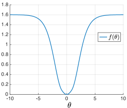
Figure 6: The image of $f$.

Since $\theta^{*}=0$, we have $\pi_{\theta^{*}}=1/2$, and for all $\left|\pi_{\theta}-\pi_{\theta^{*}}\right|>0.2$,

$$\left|\frac{df(\theta)}{d\theta}\right| =\left|\frac{d\pi_{\theta}}{d\theta}\cdot\frac{df(\theta)}{d\pi_{\theta}}\right|$$ (197)

$$=\left|\pi_{\theta}\cdot\left(1-\pi_{\theta}\right)\cdot 100\cdot\left(\pi_{\theta}-\pi_{\theta^{*}}\right)^{3}\right|$$ (198)

$$=100\cdot\pi_{\theta}\cdot\left(1-\pi_{\theta}\right)\cdot\left[\left(\pi_{\theta}-\pi_{\theta^{*}}\right)^{4}\right]^{\frac{3}{4}}$$ (199)

$$=100\cdot\pi_{\theta}\cdot\left(1-\pi_{\theta}\right)\cdot\left[f(\theta)-f(\theta^{*})\right]^{1-\frac{1}{4}},$$ (200)

which means $f$ satisfies NŁ inequality with $\xi=1/4<1/2$. For all $\left|\pi_{\theta}-\pi_{\theta^{*}}\right|\leq 1$, the Hessian of $f$ is,

$$\left|\frac{d^{2}f(\theta)}{d\theta^{2}}\right| =\left|\frac{d}{d\theta}\left\{100\cdot\pi_{\theta}\cdot\left(1-\pi_{\theta}\right)\cdot\left(\pi_{\theta}-\pi_{\theta^{*}}\right)\right\}\right|$$ (201)

$$=\left|100\cdot\pi_{\theta}\cdot\left(1-\pi_{\theta}\right)\cdot\left(\pi_{\theta}-\pi_{\theta^{*}}\right)\cdot\left(1-2\pi_{\theta}\right)+100\cdot\pi_{\theta}^{2}\cdot\left(1-\pi_{\theta}\right)^{2}\right|.$$ (202)

As $\pi_{\theta}\to\pi_{\theta^{*}}=1/2$, we have

$$100\cdot\pi_{\theta}\cdot\left(1-\pi_{\theta}\right)\cdot\left(\pi_{\theta}-\pi_{\theta^{*}}\right)\cdot\left(1-2\pi_{\theta}\right)\to 0,$$ (203)

and,

$$100\cdot\pi_{\theta}^{2}\cdot\left(1-\pi_{\theta}\right)^{2}\to 100\cdot\frac{1}{4}\cdot\frac{1}{4}=\frac{25}{4}>0,$$ (204)

which means $\beta(\theta)\to\beta>0$ as $\theta,\theta^{\prime}\to\theta^{*}$ in Definition 3.

(4) ${\mathcal{Z}}\coloneqq\text{BD}\setminus(\text{BDE}\cup\text{BF})\not=\emptyset$. Consider minimizing the same function as in (2),

$$f(\theta)=\left\|\pi_{\theta}-y\right\|_{2}^{2},$$ (205)

where $\pi_{\theta}=\mathrm{softmax}(\theta)$, $\theta\in{\mathbb{R}}^{K}$, and $y\in(0,1)$ is a probability vector with $\min_{a}{y(a)}>0$, i.e., $y$ is bounded away from the boundary of probability simplex. We show that $f$ is non-convex using one example. Let $y=(1/2,1/4,1/4)^{\top}$. Let $\theta_{1}=(0,0,0)^{\top}$, $\pi_{\theta_{1}}=\mathrm{softmax}(\theta_{1})=(1/3,1/3,1/3)^{\top}$, $\theta_{2}=(\log{4},\log{36},\log{100})^{\top}$, and $\pi_{\theta_{2}}=\mathrm{softmax}(\theta_{2})=(4/140,36/140,100/140)^{\top}$. We have,

$$f(\theta_{1})=\left\|\pi_{\theta_{1}}-y\right\|_{2}^{2}=\frac{1}{24},\text{ and }f(\theta_{2})=\left\|\pi_{\theta_{2}}-y\right\|_{2}^{2}=\frac{613}{1400}.$$ (206)

Denote $\bar{\theta}=\frac{1}{2}\cdot\left(\theta_{1}+\theta_{2}\right)=(\log{2},\log{6},\log{10})^{\top}$ we have $\pi_{\bar{\theta}}=\mathrm{softmax}(\bar{\theta})=\left(2/18,6/18,10/18\right)^{\top}$ and

$$f(\bar{\theta}) =\left\|\pi_{\bar{\theta}}-y\right\|_{2}^{2}=\frac{163}{648}.$$ (207)

Therefore we have,

$$\frac{1}{2}\cdot\left(f(\theta_{1})+f(\theta_{2})\right)=\frac{1007}{4200}=\frac{27189}{113400}<\frac{28525}{113400}=\frac{163}{648}=f(\bar{\theta}),$$ (208)

which means $f$ is non-convex. Similar as (2), we have the Hessian of $f$,

$$S_{(i,j)} =\underbrace{\delta_{ij}\pi_{\theta}(j)\cdot\left[\pi_{\theta}(i)-y(i)-\pi_{\theta}^{\top}\left(\pi_{\theta}-y\right)\right]}_{\text{(a)}}-\underbrace{\pi_{\theta}(i)\pi_{\theta}(j)\cdot\left[\pi_{\theta}(i)-y(i)-\pi_{\theta}^{\top}\left(\pi_{\theta}-y\right)\right]}_{\text{(b)}}$$ (209)

$$\quad-\underbrace{\pi_{\theta}(i)\pi_{\theta}(j)\cdot\left[\pi_{\theta}(j)-y(j)-\pi_{\theta}^{\top}\left(\pi_{\theta}-y\right)\right]}_{\text{(c)}}+\underbrace{\pi_{\theta}(i)\pi_{\theta}(j)\cdot\left[\delta_{ij}-\pi_{\theta}(i)-\pi_{\theta}(j)+\pi_{\theta}^{\top}\pi_{\theta}\right]}_{\text{(d)}},$$ (210)

where $(a)=(b)=(c)=0$ when $\pi_{\theta}=y$. Hence, at the optimal point $\theta^{*}$, we have,

$$S=\frac{1}{128}\cdot\begin{bmatrix}12&-6&-6\vspace{1ex}\\ -6&7&-1\vspace{1ex}\\ -6&-1&7\end{bmatrix},$$ (211)

and the eigenvalues of $S$ are $0$, $\frac{1}{16}$, and $\frac{9}{64}$. Thus as $\theta,\theta^{\prime}\rightarrow\theta^{*}$, the Hessian spectral radius of $f$ satisfies $\beta(\theta)\rightarrow\beta=\frac{9}{64}$. ∎

Proposition 4. The convex function $f:x\mapsto|x|^{p}$ with $p>1$ satisfies the NŁ inequality with $\xi=1/p$ and the NS property with $\beta(x)\leq c_{1}\cdot\delta(x)^{1-2\xi}$.

Proof.

For $p>1$, $f$ is differentiable, and we have,

$$\left|f^{\prime}(x)\right|=\left|p\cdot|x|^{p-1}\cdot\operatorname{sign}\{x\}\right|=p\cdot\left(\left|x\right|^{p}\right)^{\frac{p-1}{p}}=p\cdot\left(f(x)-f(0)\right)^{1-\frac{1}{p}},$$ (212)

which means $f$ satisfies NŁ inequality with $\xi=1/p$. On the other hand, the Hessian of $f$ is,

$$\left|f^{\prime\prime}(x)\right|=\left|p\cdot(p-1)\cdot\left|x\right|^{p-2}\right|=p\cdot(p-1)\cdot(\left|x\right|^{p})^{\frac{p-2}{p}}=p\cdot(p-1)\cdot(f(x)-f(0))^{1-\frac{2}{p}}.\qed$$

Appendix B Proofs for Section 5

B.1 One-state MDPs

Lemma 1 (NŁ) . Let $a^{*}$ be the uniqe optimal action. Denote $\pi^{*}=\operatorname*{arg\,max}_{\pi\in\Delta}{\pi^{\top}r}$. Then,

$$\left\|\frac{d\pi_{\theta}^{\top}r}{d\theta}\right\|_{2}\geq\pi_{\theta}(a^{*})\cdot(\pi^{*}-\pi_{\theta})^{\top}r.$$ (213)

Proof.

See the proof in (Mei et al., 2020b, Lemma 3). We include a proof for completeness.

Using the expression of the policy gradient,

$$\left\|\frac{d\pi_{\theta}^{\top}r}{d\theta}\right\|_{2} =\left(\sum_{a\in{\mathcal{A}}}{\left[\pi_{\theta}(a)\cdot(r(a)-\pi_{\theta}^{\top}r)\right]^{2}}\right)^{\frac{1}{2}}$$ (214)

$$\geq\pi_{\theta}(a^{*})\cdot(r(a^{*})-\pi_{\theta}^{\top}r).\qed$$ (215)

Lemma 2 (NS) . Let $\pi_{\theta}=\mathrm{softmax}(\theta)$ and $\pi_{\theta^{\prime}}=\mathrm{softmax}(\theta^{\prime})$. Denote $\theta_{\zeta}\coloneqq\theta+\zeta\cdot(\theta^{\prime}-\theta)$ with some $\zeta\in[0,1]$. For any $r\in\left[0,1\right]^{K}$, $\theta\mapsto\pi_{\theta}^{\top}r$ is $\beta(\theta_{\zeta})$ non-uniform smooth with $\beta(\theta_{\zeta})=3\cdot\Big{\|}\frac{d\pi_{\theta_{\zeta}}^{\top}r}{d{\theta_{\zeta}}}\Big{\|}_{2}$.

Proof.

Let $S:=S(r,\theta)\in\mathbb{R}^{K\times K}$ be the second derivative of the value map $\theta\mapsto\pi_{\theta}^{\top}r$. By Taylor’s theorem, it suffices to show that the spectral radius of $S$ is upper bounded. Denote $H(\pi_{\theta})\coloneqq\text{diag}(\pi_{\theta})-\pi_{\theta}\pi_{\theta}^{\top}$ as the Jacobian of $\theta\mapsto\mathrm{softmax}(\theta)$. Now, by its definition we have

$$S =\frac{d}{d\theta}\left\{\frac{d\pi_{\theta}^{\top}r}{d\theta}\right\}$$ (216)

$$=\frac{d}{d\theta}\left\{H(\pi_{\theta})r\right\}$$ (217)

$$=\frac{d}{d\theta}\left\{(\text{diag}(\pi_{\theta})-\pi_{\theta}\pi_{\theta}^{\top})r\right\}.$$ (218)

Continuing with our calculation fix $i,j\in[K]$. Then,

$$S_{(i,j)} =\frac{d\{\pi_{\theta}(i)\cdot(r(i)-\pi_{\theta}^{\top}r)\}}{d\theta(j)}$$ (219)

$$=\frac{d\pi_{\theta}(i)}{d\theta(j)}\cdot(r(i)-\pi_{\theta}^{\top}r)+\pi_{\theta}(i)\cdot\frac{d\{r(i)-\pi_{\theta}^{\top}r\}}{d\theta(j)}$$ (220)

$$=(\delta_{ij}\pi_{\theta}(j)-\pi_{\theta}(i)\pi_{\theta}(j))\cdot(r(i)-\pi_{\theta}^{\top}r)-\pi_{\theta}(i)\cdot(\pi_{\theta}(j)r(j)-\pi_{\theta}(j)\pi_{\theta}^{\top}r)$$ (221)

$$=\delta_{ij}\pi_{\theta}(j)\cdot(r(i)-\pi_{\theta}^{\top}r)-\pi_{\theta}(i)\pi_{\theta}(j)\cdot(r(i)-\pi_{\theta}^{\top}r)-\pi_{\theta}(i)\pi_{\theta}(j)\cdot(r(j)-\pi_{\theta}^{\top}r),$$ (222)

where

$$\delta_{ij}=\begin{cases}1,&\text{if }i=j,\\ 0,&\text{otherwise}\end{cases}$$ (223)

is Kronecker’s $\delta$-function as defined in Eq. 187. To show the bound on the spectral radius of $S$, pick $y\in{\mathbb{R}}^{K}$. Then,

$$\left|y^{\top}Sy\right| =\left|\sum\limits_{i=1}^{K}{\sum\limits_{j=1}^{K}{S_{(i,j)}\cdot y(i)\cdot y(j)}}\right|$$ (224)

$$=\left|\sum_{i}{\pi_{\theta}(i)(r(i)-\pi_{\theta}^{\top}r)y(i)^{2}}-2\sum_{i}\pi_{\theta}(i)(r(i)-\pi_{\theta}^{\top}r)y(i)\sum_{j}\pi_{\theta}(j)y(j)\right|$$ (225)

$$=\left|\left(H(\pi_{\theta})r\right)^{\top}\left(y\odot y\right)-2\cdot\left(H(\pi_{\theta})r\right)^{\top}y\cdot\left(\pi_{\theta}^{\top}y\right)\right|$$ (226)

$$\leq\left\|H(\pi_{\theta})r\right\|_{\infty}\cdot\left\|y\odot y\right\|_{1}+2\cdot\left\|H(\pi_{\theta})r\right\|_{2}\cdot\left\|y\right\|_{2}\cdot\left\|\pi_{\theta}\right\|_{1}\cdot\left\|y\right\|_{\infty}$$ (227)

$$\leq 3\cdot\left\|H(\pi_{\theta})r\right\|_{2}\cdot\left\|y\right\|_{2}^{2}.$$ (228)

According to Taylor’s theorem, $\forall\theta,\ \theta^{\prime}$,

$$\left|(\pi_{\theta^{\prime}}-\pi_{\theta})^{\top}r-\Big{\langle}\frac{d\pi_{\theta}^{\top}r}{d\theta},\theta^{\prime}-\theta\Big{\rangle}\right| =\frac{1}{2}\cdot\left|\left(\theta^{\prime}-\theta\right)^{\top}S(r,\theta_{\zeta})\left(\theta^{\prime}-\theta\right)\right|$$ (229)

$$\leq\frac{3}{2}\cdot\left\|H(\pi_{\theta_{\zeta}})r\right\|_{2}\cdot\|\theta^{\prime}-\theta\|_{2}^{2}\qquad\left(\text{by \lx@cref{creftype~refnum}{eq:non_uniform_smoothness_softmax_special_Hessian_spectral_radius}}\right)$$ (230)

$$=\frac{3}{2}\cdot\bigg{\|}\frac{d\pi_{\theta_{\zeta}}^{\top}r}{d{\theta_{\zeta}}}\bigg{\|}_{2}\cdot\|\theta^{\prime}-\theta\|_{2}^{2}.\qquad\left(\text{by \lx@cref{creftype~refnum}{lem:policy_gradient_norm_softmax}}\right)\qed$$ (231)

Lemma 3. Let

$$\theta^{\prime}=\theta+\eta\cdot\frac{d\pi_{\theta}^{\top}r}{d{\theta}}\Big{/}\left\|\frac{d\pi_{\theta}^{\top}r}{d{\theta}}\right\|_{2}.$$ (232)

Denote $\theta_{\zeta}\coloneqq\theta+\zeta\cdot(\theta^{\prime}-\theta)$ with some $\zeta\in[0,1]$. We have, for all $\eta\in(0,1/3)$,

$$\bigg{\|}\frac{d\pi_{\theta_{\zeta}}^{\top}r}{d{\theta_{\zeta}}}\bigg{\|}_{2}\leq\frac{1}{1-3\eta}\cdot\left\|\frac{d\pi_{\theta}^{\top}r}{d{\theta}}\right\|_{2}.$$ (233)

Proof.

Denote $\zeta_{1}\coloneqq\zeta$. Also denote $\theta_{\zeta_{2}}\coloneqq\theta+\zeta_{2}\cdot(\theta_{\zeta_{1}}-\theta)$ with some $\zeta_{2}\in[0,1]$. We have,

$$\left\|\frac{d\pi_{\theta_{\zeta_{1}}}^{\top}r}{d{\theta_{\zeta_{1}}}}-\frac{d\pi_{\theta}^{\top}r}{d{\theta}}\right\|_{2}=\left\|\int_{0}^{1}\bigg{\langle}\frac{d^{2}\{\pi_{\theta_{\zeta_{2}}}^{\top}r\}}{d{\theta_{\zeta_{2}}^{2}}},\theta_{\zeta_{1}}-\theta\bigg{\rangle}d\zeta_{2}\right\|_{2}$$ (234)

$$\leq\int_{0}^{1}\left\|\frac{d^{2}\{\pi_{\theta_{\zeta_{2}}}^{\top}r\}}{d{\theta_{\zeta_{2}}^{2}}}\right\|_{2}\cdot\left\|\theta_{\zeta_{1}}-\theta\right\|_{2}d\zeta_{2}$$ (235)

$$\leq\int_{0}^{1}3\cdot\left\|\frac{d\pi_{\theta_{\zeta_{2}}}^{\top}r}{d{\theta_{\zeta_{2}}}}\right\|_{2}\cdot\zeta_{1}\cdot\left\|\theta^{\prime}-\theta\right\|_{2}d\zeta_{2}\qquad\left(\text{by \lx@cref{creftype~refnum}{eq:non_uniform_smoothness_softmax_special_Hessian_spectral_radius}}\right)$$ (236)

$$\leq\int_{0}^{1}3\cdot\left\|\frac{d\pi_{\theta_{\zeta_{2}}}^{\top}r}{d{\theta_{\zeta_{2}}}}\right\|_{2}\cdot\eta\ d\zeta_{2},\qquad\left(\zeta_{1}\in[0,1],\text{ using }\theta^{\prime}=\theta+\eta\cdot\frac{d\pi_{\theta}^{\top}r}{d{\theta}}\bigg{/}\left\|\frac{d\pi_{\theta}^{\top}r}{d{\theta}}\right\|_{2}\right)$$ (237)

where the second last inequality is because of the Hessian is symmetric, and its operator norm is equal to its spectral radius. Therefore we have,

$$\left\|\frac{d\pi_{\theta_{\zeta_{1}}}^{\top}r}{d{\theta_{\zeta_{1}}}}\right\|_{2} \leq\left\|\frac{d\pi_{\theta}^{\top}r}{d{\theta}}\right\|_{2}+\left\|\frac{d\pi_{\theta_{\zeta_{1}}}^{\top}r}{d{\theta_{\zeta_{1}}}}-\frac{d\pi_{\theta}^{\top}r}{d{\theta}}\right\|_{2}\qquad\left(\text{by triangle inequality}\right)$$ (238)

$$\leq\left\|\frac{d\pi_{\theta}^{\top}r}{d{\theta}}\right\|_{2}+3\eta\cdot\int_{0}^{1}\left\|\frac{d\pi_{\theta_{\zeta_{2}}}^{\top}r}{d{\theta_{\zeta_{2}}}}\right\|_{2}d\zeta_{2}.\qquad\left(\text{by \lx@cref{creftype~refnum}{eq:non_uniform_smoothness_intermediate_policy_gradient_norm_special_1}}\right)$$ (239)

Denote $\theta_{\zeta_{3}}\coloneqq\theta+\zeta_{3}\cdot(\theta_{\zeta_{2}}-\theta)$ with some $\zeta_{3}\in[0,1]$. Using similar calculation as in Eq. 234, we have,

$$\left\|\frac{d\pi_{\theta_{\zeta_{2}}}^{\top}r}{d{\theta_{\zeta_{2}}}}\right\|_{2} \leq\left\|\frac{d\pi_{\theta}^{\top}r}{d{\theta}}\right\|_{2}+\left\|\frac{d\pi_{\theta_{\zeta_{2}}}^{\top}r}{d{\theta_{\zeta_{2}}}}-\frac{d\pi_{\theta}^{\top}r}{d{\theta}}\right\|_{2}$$ (240)

$$\leq\left\|\frac{d\pi_{\theta}^{\top}r}{d{\theta}}\right\|_{2}+3\eta\cdot\int_{0}^{1}\left\|\frac{d\pi_{\theta_{\zeta_{3}}}^{\top}r}{d{\theta_{\zeta_{3}}}}\right\|_{2}d\zeta_{3}.$$ (241)

Combining Eqs. 238 and 240, we have,

$$\left\|\frac{d\pi_{\theta_{\zeta_{1}}}^{\top}r}{d{\theta_{\zeta_{1}}}}\right\|_{2}\leq\left(1+3\eta\right)\cdot\left\|\frac{d\pi_{\theta}^{\top}r}{d{\theta}}\right\|_{2}+\left(3\eta\right)^{2}\cdot\int_{0}^{1}\int_{0}^{1}\left\|\frac{d\pi_{\theta_{\zeta_{3}}}^{\top}r}{d{\theta_{\zeta_{3}}}}\right\|_{2}d\zeta_{3}d\zeta_{2},$$ (242)

which implies,

$$\left\|\frac{d\pi_{\theta_{\zeta_{1}}}^{\top}r}{d{\theta_{\zeta_{1}}}}\right\|_{2} \leq\left[\sum_{i=0}^{\infty}{(3\eta)^{i}}\right]\cdot\left\|\frac{d\pi_{\theta}^{\top}r}{d{\theta}}\right\|_{2}$$ (243)

$$=\frac{1}{1-3\eta}\cdot\left\|\frac{d\pi_{\theta}^{\top}r}{d{\theta}}\right\|_{2}.\qquad\left(\eta\in(0,1/3)\right)\qed$$ (244)

Lemma 4 (Non-vanishing NŁ coefficient) . Using normalized policy gradient method, we have $\inf_{t\geq 1}\pi_{\theta_{t}}(a^{*})>0$.

Proof.

The proof is similar to Mei et al. (2020b, Lemma 5). Let

$$c=\frac{K}{2\Delta}\cdot\left(1-\frac{\Delta}{K}\right)$$ (245)

and

$$\Delta=r(a^{*})-\max_{a\not=a^{*}}{r(a)}>0$$ (246)

denote the reward gap of $r$. We will prove that $\inf_{t\geq 1}\pi_{\theta_{t}}(a^{*})=\min_{1\leq t\leq t_{0}}{\pi_{\theta_{t}}(a^{*})}$, where $t_{0}=\min\{t:\pi_{\theta_{t}}(a^{*})\geq\frac{c}{c+1}\}$. Note that $t_{0}$ depends only on $\theta_{1}$ and $c$, and $c$ depends only on the problem. Define the following regions,

$${\mathcal{R}}_{1} =\left\{\theta:\frac{d\pi_{\theta}^{\top}r}{d\theta(a^{*})}\geq\frac{d\pi_{\theta}^{\top}r}{d\theta(a)},\ \forall a\not=a^{*}\right\},$$ (247)

$${\mathcal{R}}_{2} =\left\{\theta:\pi_{\theta}(a^{*})\geq\pi_{\theta}(a),\ \forall a\not=a^{*}\right\}\,,$$ (248)

$${\mathcal{N}}_{c} =\left\{\theta:\pi_{\theta}(a^{*})\geq\frac{c}{c+1}\right\}.$$ (249)

We make the following three-part claim.

Claim 6.

The following hold :

a)

Following a NPG update $\theta_{t+1}=\theta_{t}+\eta\cdot\frac{d\pi_{\theta_{t}}^{\top}r}{d{\theta_{t}}}\Big{/}\Big{\|}\frac{d\pi_{\theta_{t}}^{\top}r}{d{\theta_{t}}}\Big{\|}_{2}$, if $\theta_{t}\in{\mathcal{R}}_{1}$, then (i) $\theta_{t+1}\in{\mathcal{R}}_{1}$ and (ii) $\pi_{\theta_{t+1}}(a^{*})\geq\pi_{\theta_{t}}(a^{*})$.

b)

We have ${\mathcal{R}}_{2}\subset{\mathcal{R}}_{1}$ and ${\mathcal{N}}_{c}\subset{\mathcal{R}}_{1}$.

c)

For $\eta=1/6$, there exists a finite time $t_{0}\geq 1$, such that $\theta_{t_{0}}\in{\mathcal{N}}_{c}$, and thus $\theta_{t_{0}}\in{\mathcal{R}}_{1}$, which implies that $\inf_{t\geq 1}\pi_{\theta_{t}}(a^{*})=\min_{1\leq t\leq t_{0}}{\pi_{\theta_{t}}(a^{*})}$..

Claim a)

Part (i): We want to show that if $\theta_{t}\in{\mathcal{R}}_{1}$, then $\theta_{t+1}\in{\mathcal{R}}_{1}$. Let

$${\mathcal{R}}_{1}(a) =\left\{\theta:\frac{d\pi_{\theta}^{\top}r}{d\theta(a^{*})}\geq\frac{d\pi_{\theta}^{\top}r}{d\theta(a)}\right\}.$$ (250)

Note that ${\mathcal{R}}_{1}=\cap_{a\neq a^{*}}{\mathcal{R}}_{1}(a)$. Pick $a\neq a^{*}$. Clearly, it suffices to show that if $\theta_{t}\in{\mathcal{R}}_{1}(a)$ then $\theta_{t+1}\in{\mathcal{R}}_{1}(a)$. Hence, suppose that $\theta_{t}\in{\mathcal{R}}_{1}(a)$. We consider two cases.

Case (a): $\pi_{\theta_{t}}(a^{*})\geq\pi_{\theta_{t}}(a)$. Since $\pi_{\theta_{t}}(a^{*})\geq\pi_{\theta_{t}}(a)$, we also have $\theta_{t}(a^{*})\geq\theta_{t}(a)$. After an update of the parameters,

$$\theta_{t+1}(a^{*}) =\theta_{t}(a^{*})+\frac{\eta}{\Big{\|}\frac{d\pi_{\theta_{t}}^{\top}r}{d{\theta_{t}}}\Big{\|}_{2}}\cdot\frac{d\pi_{\theta_{t}}^{\top}r}{d\theta_{t}(a^{*})}$$ (251)

$$\geq\theta_{t}(a)+\frac{\eta}{\Big{\|}\frac{d\pi_{\theta_{t}}^{\top}r}{d{\theta_{t}}}\Big{\|}_{2}}\cdot\frac{d\pi_{\theta_{t}}^{\top}r}{d\theta_{t}(a)}$$ (252)

$$=\theta_{t+1}(a),$$ (253)

which implies that $\pi_{\theta_{t+1}}(a^{*})\geq\pi_{\theta_{t+1}}(a)$. Since $r(a^{*})-\pi_{\theta_{t+1}}^{\top}r>0$ and $r(a^{*})>r(a)$,

$$\pi_{\theta_{t+1}}(a^{*})\cdot\left(r(a^{*})-\pi_{\theta_{t+1}}^{\top}r\right)\geq\pi_{\theta_{t+1}}(a)\cdot\left(r(a)-\pi_{\theta_{t+1}}^{\top}r\right),$$ (254)

which is equivalent to $\frac{d\pi_{\theta_{t+1}}^{\top}r}{d\theta_{t+1}(a^{*})}\geq\frac{d\pi_{\theta_{t+1}}^{\top}r}{d\theta_{t+1}(a)}$, i.e., $\theta_{t+1}\in{\mathcal{R}}_{1}(a)$.

Case (b): Suppose now that $\pi_{\theta_{t}}(a^{*})<\pi_{\theta_{t}}(a)$. First note that for any $\theta$ and $a\neq a^{*}$, $\theta\in{\mathcal{R}}_{1}(a)$ holds if and only if

$$r(a^{*})-r(a) \geq\left(1-\frac{\pi_{\theta}(a^{*})}{\pi_{\theta}(a)}\right)\cdot\left(r(a^{*})-\pi_{\theta}^{\top}r\right).$$ (255)

Indeed, from the condition $\frac{d\pi_{\theta}^{\top}r}{d\theta(a^{*})}\geq\frac{d\pi_{\theta}^{\top}r}{d\theta(a)}$, we get

$$\pi_{\theta}(a^{*})\cdot\left(r(a^{*})-\pi_{\theta}^{\top}r\right) \geq\pi_{\theta}(a)\cdot\left(r(a)-\pi_{\theta}^{\top}r\right)$$ (256)

$$=\pi_{\theta}(a)\cdot\left(r(a^{*})-\pi_{\theta}^{\top}r\right)-\pi_{\theta}(a)\cdot\left(r(a^{*})-r(a)\right),$$ (257)

which, after rearranging, is equivalent to Eq. 255. Hence, it suffices to show that Eq. 255 holds for $\theta_{t+1}$ provided it holds for $\theta_{t}$. From the latter condition, we get

$$r(a^{*})-r(a)\geq\left(1-\exp\left\{\theta_{t}(a^{*})-\theta_{t}(a)\right\}\right)\cdot\left(r(a^{*})-\pi_{\theta_{t}}^{\top}r\right).$$ (258)

After an update of the parameters, according to Lemma 12 (or Eq. 273 below), $\pi_{\theta_{t+1}}^{\top}r\geq\pi_{\theta_{t}}^{\top}r$, i.e.,

$$0<r(a^{*})-\pi_{\theta_{t+1}}^{\top}r\leq r(a^{*})-\pi_{\theta_{t}}^{\top}r\,.$$ (259)

On the other hand,

$$\theta_{t+1}(a^{*})-\theta_{t+1}(a) =\theta_{t}(a^{*})+\frac{\eta}{\Big{\|}\frac{d\pi_{\theta_{t}}^{\top}r}{d{\theta_{t}}}\Big{\|}_{2}}\cdot\frac{d\pi_{\theta_{t}}^{\top}r}{d\theta_{t}(a^{*})}-\theta_{t}(a)-\frac{\eta}{\Big{\|}\frac{d\pi_{\theta_{t}}^{\top}r}{d{\theta_{t}}}\Big{\|}_{2}}\cdot\frac{d\pi_{\theta_{t}}^{\top}r}{d\theta_{t}(a)}$$ (260)

$$\geq\theta_{t}(a^{*})-\theta_{t}(a),$$ (261)

which implies that

$$1-\exp\left\{\theta_{t+1}(a^{*})-\theta_{t+1}(a)\right\}\leq 1-\exp\left\{\theta_{t}(a^{*})-\theta_{t}(a)\right\}.$$ (262)

Furthermore, by our assumption that $\pi_{\theta_{t}}(a^{*})<\pi_{\theta_{t}}(a)$, we have $1-\exp\left\{\theta_{t}(a^{*})-\theta_{t}(a)\right\}=1-\frac{\pi_{\theta_{t}}(a^{*})}{\pi_{\theta_{t}}(a)}>0$. Putting things together, we get

$$\left(1-\exp\left\{\theta_{t+1}(a^{*})-\theta_{t+1}(a)\right\}\right)\cdot\left(r(a^{*})-\pi_{\theta_{t+1}}^{\top}r\right) \leq\left(1-\exp\left\{\theta_{t}(a^{*})-\theta_{t}(a)\right\}\right)\cdot\left(r(a^{*})-\pi_{\theta_{t}}^{\top}r\right)$$ (263)

$$\leq r(a^{*})-r(a),$$ (264)

which is equivalent to

$$\left(1-\frac{\pi_{\theta_{t+1}}(a^{*})}{\pi_{\theta_{t+1}}(a)}\right)\cdot\left(r(a^{*})-\pi_{\theta_{t+1}}^{\top}r\right)\leq r(a^{*})-r(a),$$ (265)

and thus by our previous remark, $\theta_{t+1}\in{\mathcal{R}}_{1}(a)$, thus, finishing the proof of part (i).

Part (ii): Assume again that $\theta_{t}\in{\mathcal{R}}_{1}$. We want to show that $\pi_{\theta_{t+1}}(a^{*})\geq\pi_{\theta_{t}}(a^{*})$. Since $\theta_{t}\in{\mathcal{R}}_{1}$, we have $\frac{d\pi_{\theta_{t}}^{\top}r}{d\theta_{t}(a^{*})}\geq\frac{d\pi_{\theta_{t}}^{\top}r}{d\theta_{t}(a)},\ \forall a\not=a^{*}$. Hence,

$$\pi_{\theta_{t+1}}(a^{*})=\frac{\exp\left\{\theta_{t+1}(a^{*})\right\}}{\sum_{a}{\exp\left\{\theta_{t+1}(a)\right\}}}$$ (266)

$$=\frac{\exp\left\{\theta_{t}(a^{*})+\eta\cdot\frac{d\pi_{\theta_{t}}^{\top}r}{d\theta_{t}(a^{*})}\Big{/}\Big{\|}\frac{d\pi_{\theta_{t}}^{\top}r}{d{\theta_{t}}}\Big{\|}_{2}\right\}}{\sum_{a}{\exp\left\{\theta_{t}(a)+\eta\cdot\frac{d\pi_{\theta_{t}}^{\top}r}{d\theta_{t}(a)}\Big{/}\Big{\|}\frac{d\pi_{\theta_{t}}^{\top}r}{d{\theta_{t}}}\Big{\|}_{2}\right\}}}$$ (267)

$$\geq\frac{\exp\left\{\theta_{t}(a^{*})+\eta\cdot\frac{d\pi_{\theta_{t}}^{\top}r}{d\theta_{t}(a^{*})}\Big{/}\Big{\|}\frac{d\pi_{\theta_{t}}^{\top}r}{d{\theta_{t}}}\Big{\|}_{2}\right\}}{\sum_{a}{\exp\left\{\theta_{t}(a)+\eta\cdot\frac{d\pi_{\theta_{t}}^{\top}r}{d\theta_{t}(a^{*})}\Big{/}\Big{\|}\frac{d\pi_{\theta_{t}}^{\top}r}{d{\theta_{t}}}\Big{\|}_{2}\right\}}}\qquad\left(\text{using }\frac{d\pi_{\theta_{t}}^{\top}r}{d\theta_{t}(a^{*})}\geq\frac{d\pi_{\theta_{t}}^{\top}r}{d\theta_{t}(a)}\right)$$ (268)

$$=\frac{\exp\left\{\theta_{t}(a^{*})\right\}}{\sum_{a}{\exp\left\{\theta_{t}(a)\right\}}}=\pi_{\theta_{t}}(a^{*}).$$ (269)

Claim b); Claim c)

The proof of those claims are exactly the same as Mei et al. (2020b, Lemma 5), since they do not involve the update rule. ∎

Theorem 2. Using NPG $\theta_{t+1}=\theta_{t}+\eta\cdot\frac{d\pi_{\theta_{t}}^{\top}r}{d{\theta_{t}}}\Big{/}\Big{\|}\frac{d\pi_{\theta_{t}}^{\top}r}{d{\theta_{t}}}\Big{\|}_{2}$, with $\eta=1/6$, for all $t\geq 1$, we have,

$$(\pi^{*}-\pi_{\theta_{t}})^{\top}r\leq e^{-\frac{c\cdot(t-1)}{12}}\cdot\left(\pi^{*}-\pi_{\theta_{1}}\right)^{\top}r,$$ (270)

where $c=\inf_{t\geq 1}\pi_{\theta_{t}}(a^{*})>0$ is from Lemma 4, and $c$ is a constant that depends on $r$ and $\theta_{1}$, but not on the time $t$.

Proof.

Denote $\theta_{\zeta_{t}}\coloneqq\theta_{t}+\zeta_{t}\cdot(\theta_{t+1}-\theta_{t})$ with some $\zeta_{t}\in[0,1]$. According to Lemma 2,

$$\left|(\pi_{\theta_{t+1}}-\pi_{\theta_{t}})^{\top}r-\Big{\langle}\frac{d\pi_{\theta_{t}}^{\top}r}{d\theta_{t}},\theta_{t+1}-\theta_{t}\Big{\rangle}\right|\leq\frac{3}{2}\cdot\bigg{\|}\frac{d\pi_{\theta_{\zeta_{t}}}^{\top}r}{d{\theta_{\zeta_{t}}}}\bigg{\|}_{2}\cdot\|\theta_{t+1}-\theta_{t}\|_{2}^{2}$$ (271)

$$\leq\frac{3}{2}\cdot\frac{1}{1-3\eta}\cdot\left\|\frac{d\pi_{\theta_{t}}^{\top}r}{d{\theta_{t}}}\right\|_{2}\cdot\|\theta_{t+1}-\theta_{t}\|_{2}^{2},\qquad\left(\eta=1/6,\text{ by \lx@cref{creftype~refnum}{lem:non_uniform_smoothness_intermediate_policy_gradient_norm_special}}\right)$$ (272)

which implies,

$$\pi_{\theta_{t}}^{\top}r-\pi_{\theta_{t+1}}^{\top}r\leq-\Big{\langle}\frac{d\pi_{\theta_{t}}^{\top}r}{d\theta_{t}},\theta_{t+1}-\theta_{t}\Big{\rangle}+\frac{3}{2\cdot(1-3\eta)}\cdot\left\|\frac{d\pi_{\theta_{t}}^{\top}r}{d{\theta_{t}}}\right\|_{2}\cdot\|\theta_{t+1}-\theta_{t}\|_{2}^{2}$$ (273)

$$=-\eta\cdot\left\|\frac{d\pi_{\theta_{t}}^{\top}r}{d\theta_{t}}\right\|_{2}+\frac{3\cdot\eta^{2}}{2\cdot(1-3\eta)}\cdot\left\|\frac{d\pi_{\theta_{t}}^{\top}r}{d\theta_{t}}\right\|_{2}\qquad\left(\text{using }\theta_{t+1}=\theta_{t}+\eta\cdot\frac{d\pi_{\theta_{t}}^{\top}r}{d\theta_{t}}\bigg{/}\left\|\frac{d\pi_{\theta_{t}}^{\top}r}{d{\theta_{t}}}\right\|_{2}\right)$$ (274)

$$=-\frac{1}{12}\cdot\left\|\frac{d\pi_{\theta_{t}}^{\top}r}{d\theta_{t}}\right\|_{2}\qquad\qquad\left(\text{using }\eta=1/6\right)$$ (275)

$$\leq-\frac{1}{12}\cdot\pi_{\theta_{t}}(a^{*})\cdot(\pi^{*}-\pi_{\theta_{t}})^{\top}r\qquad\left(\text{by \lx@cref{creftype~refnum}{lem:non_uniform_lojasiewicz_softmax_special}}\right)$$ (276)

$$\leq-\frac{1}{12}\cdot\inf_{t\geq 1}\pi_{\theta_{t}}(a^{*})\cdot(\pi^{*}-\pi_{\theta_{t}})^{\top}r.$$ (277)

According to Eq. 273, we have,

$$\left(\pi^{*}-\pi_{\theta_{t}}\right)^{\top}r \leq\left(1-\frac{c}{12}\right)\cdot\left(\pi^{*}-\pi_{\theta_{t-1}}\right)^{\top}r\qquad\left(c\coloneqq\inf_{t\geq 1}\pi_{\theta_{t}}(a^{*})>0\right)$$ (278)

$$\leq\exp{\left\{-c/12\right\}}\cdot\left(\pi^{*}-\pi_{\theta_{t-1}}\right)^{\top}r$$ (279)

$$\leq\exp{\left\{-(t-1)\cdot c/12\right\}}\cdot\left(\pi^{*}-\pi_{\theta_{1}}\right)^{\top}r.\qed$$ (280)

B.2 General MDPs

Lemma 5 (NŁ) . Denote $S\coloneqq|{\mathcal{S}}|$ as the total number of states. We have, for all $\theta\in{\mathbb{R}}^{{\mathcal{S}}\times{\mathcal{A}}}$,

$$\left\|\frac{\partial V^{\pi_{\theta}}(\mu)}{\partial\theta}\right\|_{2}\geq\frac{\min_{s}{\pi_{\theta}(a^{*}(s)|s)}}{\sqrt{S}\cdot\left\|d_{\rho}^{\pi^{*}}/d_{\mu}^{\pi_{\theta}}\right\|_{\infty}}\cdot\left(V^{*}(\rho)-V^{\pi_{\theta}}(\rho)\right),$$ (281)

where $a^{*}(s)$ is the action that $\pi^{*}$ selects in state $s$.

Proof.

See the proof in (Mei et al., 2020b, Lemma 8). We include a proof for completeness. We have,

$$\left\|\frac{\partial V^{\pi_{\theta}}(\mu)}{\partial\theta}\right\|_{2}=\left[\sum_{s,a}\left(\frac{\partial V^{\pi_{\theta}}(\mu)}{\partial\theta(s,a)}\right)^{2}\right]^{\frac{1}{2}}$$ (282)

$$\geq\left[\sum_{s}\left(\frac{\partial V^{\pi_{\theta}}(\mu)}{\partial\theta(s,a^{*}(s))}\right)^{2}\right]^{\frac{1}{2}}$$ (283)

$$\geq\frac{1}{\sqrt{S}}\sum_{s}\left|\frac{\partial V^{\pi_{\theta}}(\mu)}{\partial\theta(s,a^{*}(s))}\right|\qquad\left(\text{by Cauchy-Schwarz, }\|x\|_{1}=|\langle{\mathbf{1}},\ |x|\rangle|\leq\|{\mathbf{1}}\|_{2}\cdot\|x\|_{2}\right)$$ (284)

$$=\frac{1}{1-\gamma}\cdot\frac{1}{\sqrt{S}}\sum_{s}\left|d_{\mu}^{\pi_{\theta}}(s)\cdot\pi_{\theta}(a^{*}(s)|s)\cdot A^{\pi_{\theta}}(s,a^{*}(s))\right|\qquad\left(\text{by \lx@cref{creftype~refnum}{lem:policy_gradient_softmax}}\right)$$ (285)

$$=\frac{1}{1-\gamma}\cdot\frac{1}{\sqrt{S}}\sum_{s}d_{\mu}^{\pi_{\theta}}(s)\cdot\pi_{\theta}(a^{*}(s)|s)\cdot\left|A^{\pi_{\theta}}(s,a^{*}(s))\right|.\qquad\left(\text{because }d_{\mu}^{\pi_{\theta}}(s)\geq 0\text{ and }\pi_{\theta}(a^{*}(s)|s)\geq 0\right)$$ (286)

Define the distribution mismatch coefficient as $\bigg{\|}\frac{d_{\rho}^{\pi^{*}}}{d_{\mu}^{\pi_{\theta}}}\bigg{\|}_{\infty}=\max_{s}{\frac{d_{\rho}^{\pi^{*}}(s)}{d_{\mu}^{\pi_{\theta}}(s)}}$. We have,

$$\left\|\frac{\partial V^{\pi_{\theta}}(\mu)}{\partial\theta}\right\|_{2} \geq\frac{1}{1-\gamma}\cdot\frac{1}{\sqrt{S}}\sum_{s}\frac{d_{\mu}^{\pi_{\theta}}(s)}{d_{\rho}^{\pi^{*}}(s)}\cdot d_{\rho}^{\pi^{*}}(s)\cdot\pi_{\theta}(a^{*}(s)|s)\cdot\left|A^{\pi_{\theta}}(s,a^{*}(s))\right|$$ (287)

$$\geq\frac{1}{1-\gamma}\cdot\frac{1}{\sqrt{S}}\cdot\left\|\frac{d_{\rho}^{\pi^{*}}}{d_{\mu}^{\pi_{\theta}}}\right\|_{\infty}^{-1}\cdot\min_{s}{\pi_{\theta}(a^{*}(s)|s)}\cdot\sum_{s}{d_{\rho}^{\pi^{*}}(s)\cdot\left|A^{\pi_{\theta}}(s,a^{*}(s))\right|}$$ (288)

$$\geq\frac{1}{1-\gamma}\cdot\frac{1}{\sqrt{S}}\cdot\left\|\frac{d_{\rho}^{\pi^{*}}}{d_{\mu}^{\pi_{\theta}}}\right\|_{\infty}^{-1}\cdot\min_{s}{\pi_{\theta}(a^{*}(s)|s)}\cdot\sum_{s}{d_{\rho}^{\pi^{*}}(s)\cdot A^{\pi_{\theta}}(s,a^{*}(s))}$$ (289)

$$=\frac{1}{\sqrt{S}}\cdot\left\|\frac{d_{\rho}^{\pi^{*}}}{d_{\mu}^{\pi_{\theta}}}\right\|_{\infty}^{-1}\cdot\min_{s}{\pi_{\theta}(a^{*}(s)|s)}\cdot\frac{1}{1-\gamma}\sum_{s}{d_{\rho}^{\pi^{*}}(s)\sum_{a}{\pi^{*}(a|s)\cdot A^{\pi_{\theta}}(s,a)}}$$ (290)

$$=\frac{1}{\sqrt{S}}\cdot\left\|\frac{d_{\rho}^{\pi^{*}}}{d_{\mu}^{\pi_{\theta}}}\right\|_{\infty}^{-1}\cdot\min_{s}{\pi_{\theta}(a^{*}(s)|s)}\cdot\left[V^{*}(\rho)-V^{\pi_{\theta}}(\rho)\right],$$ (291)

where the one but last equality used that $\pi^{*}$ is deterministic and in state $s$ chooses $a^{*}(s)$ with probability one, and the last equality uses the performance difference formula (Lemma 17). ∎

Lemma 6 (NS) . Let 1 hold and denote $\theta_{\zeta}\coloneqq\theta+\zeta\cdot(\theta^{\prime}-\theta)$ with some $\zeta\in[0,1]$. $\theta\mapsto V^{\pi_{\theta}}(\mu)$ satisfies $\beta(\theta_{\zeta})$ non-uniform smoothness with

$$\beta(\theta_{\zeta})=\left[3+\frac{4\cdot\left(C_{\infty}-(1-\gamma)\right)}{1-\gamma}\right]\cdot\sqrt{S}\cdot\left\|\frac{\partial V^{\pi_{\theta_{\zeta}}}(\mu)}{\partial{\theta_{\zeta}}}\right\|_{2},$$ (292)

where $C_{\infty}\coloneqq\max_{\pi}{\left\|\frac{d_{\mu}^{\pi}}{\mu}\right\|_{\infty}}\leq\frac{1}{\min_{s}\mu(s)}<\infty$.

Proof.

The main part is to prove that for all $y\in{\mathbb{R}}^{SA}$ and $\theta$,

$$\left|y^{\top}\frac{\partial^{2}V^{\pi_{\theta}}(\mu)}{\partial\theta^{2}}y\right|\leq\left[3+\frac{4\cdot\left(C_{\infty}-(1-\gamma)\right)}{1-\gamma}\right]\cdot\sqrt{S}\cdot\left\|\frac{\partial V^{\pi_{\theta}}(\mu)}{\partial\theta}\right\|_{2}\cdot\|y\|_{2}^{2}.$$ (293)

We first calculate the second order derivative of $V^{\pi_{\theta}}(\mu)$ w.r.t. $\theta$.

Denote $\theta_{\alpha}=\theta+\alpha u$, where $\alpha\in{\mathbb{R}}$ and $u\in{\mathbb{R}}^{SA}$. For any $(s,a)\in{\mathcal{S}}\times{\mathcal{A}}$,

$$\frac{\partial\pi_{\theta_{\alpha}}(a|s)}{\partial\alpha}\Big{|}_{\alpha=0} =\Big{\langle}\frac{\partial\pi_{\theta_{\alpha}}(a|s)}{\partial\theta_{\alpha}}\Big{|}_{\alpha=0},\frac{\partial\theta_{\alpha}}{\partial\alpha}\Big{\rangle}$$ (294)

$$=\Big{\langle}\frac{\partial\pi_{\theta}(a|s)}{\partial\theta},u\Big{\rangle}$$ (295)

$$=\Big{\langle}\frac{\partial\pi_{\theta}(a|s)}{\partial\theta(s,\cdot)},u(s,\cdot)\Big{\rangle}.\qquad\left(\frac{\partial\pi_{\theta}(a|s)}{\partial\theta(s^{\prime},\cdot)}={\mathbf{0}},\ \forall s^{\prime}\not=s\right)$$ (296)

Similarly, for any $(s,a)\in{\mathcal{S}}\times{\mathcal{A}}$,

$$\frac{\partial^{2}\pi_{\theta_{\alpha}}(a|s)}{\partial\alpha^{2}}\Big{|}_{\alpha=0} =\Big{\langle}\frac{\partial}{\partial\theta_{\alpha}}\left\{\frac{\partial\pi_{\theta_{\alpha}}(a|s)}{\partial\alpha}\right\}\Big{|}_{\alpha=0},\frac{\partial\theta_{\alpha}}{\partial\alpha}\Big{\rangle}$$ (297)

$$=\Big{\langle}\frac{\partial^{2}\pi_{\theta_{\alpha}}(a|s)}{\partial\theta_{\alpha}^{2}}\Big{|}_{\alpha=0}\frac{\partial\theta_{\alpha}}{\partial\alpha},\frac{\partial\theta_{\alpha}}{\partial\alpha}\Big{\rangle}$$ (298)

$$=\Big{\langle}\frac{\partial^{2}\pi_{\theta}(a|s)}{\partial\theta^{2}(s,\cdot)}u(s,\cdot),u(s,\cdot)\Big{\rangle}.$$ (299)

Define $\Pi(\alpha)\in{\mathbb{R}}^{S\times SA}$ as follows,

$$\Pi(\alpha)\coloneqq\begin{bmatrix}\pi_{\theta_{\alpha}}(\cdot|1)^{\top}&{\mathbf{0}}^{\top}&\cdots&{\mathbf{0}}^{\top}\\ {\mathbf{0}}^{\top}&\pi_{\theta_{\alpha}}(\cdot|2)^{\top}&\cdots&{\mathbf{0}}^{\top}\\ \vdots&\vdots&\ddots&\vdots\\ {\mathbf{0}}^{\top}&{\mathbf{0}}^{\top}&\cdots&\pi_{\theta_{\alpha}}(\cdot|S)^{\top}\end{bmatrix}.$$ (300)

Denote ${\mathcal{P}}\in{\mathbb{R}}^{SA\times S}$ such that,

$${\mathcal{P}}_{{(sa,s^{\prime})}}\coloneqq{\mathcal{P}}(s^{\prime}|s,a).$$ (301)

Define $P(\alpha)\coloneqq\Pi(\alpha){\mathcal{P}}\in{\mathbb{R}}^{S\times S}$, where $\forall(s,s^{\prime})$,

$$\left[P(\alpha)\right]_{(s,s^{\prime})}=\sum_{a}{\pi_{\theta_{\alpha}}(a|s)\cdot{\mathcal{P}}(s^{\prime}|s,a)}.$$ (302)

The derivative w.r.t. $\alpha$ is

$$\frac{\partial P(\alpha)}{\partial\alpha} =\frac{\partial\Pi(\alpha){\mathcal{P}}}{\partial\alpha}=\frac{\partial\Pi(\alpha)}{\partial\alpha}{\mathcal{P}}.$$ (303)

And $\forall(s,s^{\prime})$, we have,

$$\left[\frac{\partial P(\alpha)}{\partial\alpha}\Big{|}_{\alpha=0}\right]_{(s,s^{\prime})}=\sum_{a}\left[\frac{\partial\pi_{\theta_{\alpha}}(a|s)}{\partial\alpha}\Big{|}_{\alpha=0}\right]\cdot{\mathcal{P}}(s^{\prime}|s,a).$$ (304)

Next, consider the state value function of $\pi_{\theta_{\alpha}}$,

$$V^{\pi_{\theta_{\alpha}}}(s) =\sum_{a}{\pi_{\theta_{\alpha}}(a|s)\cdot r(s,a)}+\gamma\sum_{a}{\pi_{\theta_{\alpha}}(a|s)\sum_{s^{\prime}}{{\mathcal{P}}(s^{\prime}|s,a)\cdot V^{\pi_{\theta_{\alpha}}}(s^{\prime})}},$$ (305)

which implies,

$$V^{\pi_{\theta_{\alpha}}}(s) =e_{s}^{\top}M(\alpha)r_{\theta_{\alpha}}$$ (306)

$$V^{\pi_{\theta_{\alpha}}}(\mu) =\mu^{\top}M(\alpha)r_{\theta_{\alpha}},$$ (307)

where

$$M(\alpha)=\left(\mathbf{Id}-\gamma P(\alpha)\right)^{-1},$$ (308)

and $r_{\theta_{\alpha}}\in{\mathbb{R}}^{S}$ is given by

$$r_{\theta_{\alpha}}=\Pi(\alpha)r,$$ (309)

where $r\in{\mathbb{R}}^{SA}$. Taking derivative w.r.t. $\alpha$ in Eq. 307,

$$\frac{\partial V^{\pi_{\theta_{\alpha}}}(\mu)}{\partial\alpha} =\gamma\cdot\mu^{\top}M(\alpha)\frac{\partial P(\alpha)}{\partial\alpha}M(\alpha)r_{\theta_{\alpha}}+\mu^{\top}M(\alpha)\frac{\partial r_{\theta_{\alpha}}}{\partial\alpha}$$ (310)

$$=\mu^{\top}M(\alpha)\left[\gamma\cdot\frac{\partial P(\alpha)}{\partial\alpha}M(\alpha)r_{\theta_{\alpha}}+\frac{\partial r_{\theta_{\alpha}}}{\partial\alpha}\right]$$ (311)

$$=\mu^{\top}M(\alpha)\left[\gamma\cdot\frac{\partial\Pi(\alpha)}{\partial\alpha}{\mathcal{P}}M(\alpha)r_{\theta_{\alpha}}+\frac{\partial\Pi(\alpha)}{\partial\alpha}r\right]\qquad\left(\text{by \lx@cref{creftypeplural~refnum}{eq:non_uniform_smoothness_softmax_general_intermediate_P_PI_first_derivative_matrix} and~\lx@cref{refnum}{eq:non_uniform_moothness_softmax_general_intermediate_reward_def_matrix}}\right)$$ (312)

$$=\mu^{\top}M(\alpha)\frac{\partial\Pi(\alpha)}{\partial\alpha}Q^{\pi_{\theta_{\alpha}}},$$ (313)

where $Q^{\pi_{\theta_{\alpha}}}\in{\mathbb{R}}^{SA}$ is the state-action value and it satisfies,

$$Q^{\pi_{\theta_{\alpha}}} =r+\gamma\cdot{\mathcal{P}}M(\alpha)r_{\theta_{\alpha}}$$ (314)

$$=r+\gamma\cdot{\mathcal{P}}V^{\pi_{\theta_{\alpha}}}.\qquad\left(\text{by \lx@cref{creftype~refnum}{eq:state_value_bellman_equation_s}}\right)$$ (315)

Similarly, taking second derivative w.r.t. $\alpha$,

$$\frac{\partial^{2}V^{\pi_{\theta_{\alpha}}}(\mu)}{\partial\alpha^{2}}=2\gamma^{2}\cdot\mu^{\top}M(\alpha)\frac{\partial P(\alpha)}{\partial\alpha}M(\alpha)\frac{\partial P(\alpha)}{\partial\alpha}M(\alpha)r_{\theta_{\alpha}}+\gamma\cdot\mu^{\top}M(\alpha)\frac{\partial^{2}P(\alpha)}{\partial\alpha^{2}}M(\alpha)r_{\theta_{\alpha}}$$ (316)

$$\qquad+2\gamma\cdot\mu^{\top}M(\alpha)\frac{\partial P(\alpha)}{\partial\alpha}M(\alpha)\frac{\partial r_{\theta_{\alpha}}}{\partial\alpha}+\mu^{\top}M(\alpha)\frac{\partial^{2}r_{\theta_{\alpha}}}{\partial\alpha^{2}}$$ (317)

$$=2\gamma\cdot\mu^{\top}M(\alpha)\frac{\partial P(\alpha)}{\partial\alpha}M(\alpha)\frac{\partial\Pi(\alpha)}{\partial\alpha}\left(\gamma\cdot{\mathcal{P}}M(\alpha)r_{\theta_{\alpha}}+r\right)+\mu^{\top}M(\alpha)\frac{\partial^{2}\Pi(\alpha)}{\partial\alpha^{2}}\left(\gamma\cdot{\mathcal{P}}M(\alpha)r_{\theta_{\alpha}}+r\right)$$ (318)

$$=2\gamma\cdot\mu^{\top}M(\alpha)\frac{\partial P(\alpha)}{\partial\alpha}M(\alpha)\frac{\partial\Pi(\alpha)}{\partial\alpha}Q^{\pi_{\theta_{\alpha}}}+\mu^{\top}M(\alpha)\frac{\partial^{2}\Pi(\alpha)}{\partial\alpha^{2}}Q^{\pi_{\theta_{\alpha}}}.$$ (319)

For the last term, we have,

$$\left[\frac{\partial^{2}\Pi(\alpha)}{\partial\alpha^{2}}Q^{\pi_{\theta_{\alpha}}}\Big{|}_{\alpha=0}\right]_{(s)} =\sum_{a}{\frac{\partial^{2}\pi_{\theta_{\alpha}}(a|s)}{\partial\alpha^{2}}\Big{|}_{\alpha=0}\cdot Q^{\pi_{\theta}}(s,a)}$$ (320)

$$=\sum_{a}{\Big{\langle}\frac{\partial^{2}\pi_{\theta}(a|s)}{\partial\theta^{2}(s,\cdot)}u(s,\cdot),u(s,\cdot)\Big{\rangle}\cdot Q^{\pi_{\theta}}(s,a)}\qquad\left(\text{by \lx@cref{creftype~refnum}{eq:non_uniform_smoothness_softmax_general_intermediate_pi_second_derivative}}\right)$$ (321)

$$=u(s,\cdot)^{\top}\left[\sum_{a}{\frac{\partial^{2}\pi_{\theta}(a|s)}{\partial\theta^{2}(s,\cdot)}\cdot Q^{\pi_{\theta}}(s,a)}\right]u(s,\cdot).$$ (322)

Let $S(a,\theta)=\frac{\partial^{2}\pi_{\theta}(a|s)}{\partial\theta^{2}(s,\cdot)}\in{\mathbb{R}}^{A\times A}$. $\forall i,j\in[A]$, the value of $S(a,\theta)$ is,

$$S_{(i,j)}=\frac{\partial\{\delta_{ia}\pi_{\theta}(a|s)-\pi_{\theta}(a|s)\pi_{\theta}(i|s)\}}{\partial\theta(s,j)}$$ (323)

$$=\delta_{ia}\cdot\left[\delta_{ja}\pi_{\theta}(a|s)-\pi_{\theta}(a|s)\pi_{\theta}(j|s)\right]-\pi_{\theta}(a|s)\cdot\left[\delta_{ij}\pi_{\theta}(j|s)-\pi_{\theta}(i|s)\pi_{\theta}(j|s)\right]-\pi_{\theta}(i|s)\cdot\left[\delta_{ja}\pi_{\theta}(a|s)-\pi_{\theta}(a|s)\pi_{\theta}(j|s)\right],$$ (324)

where the $\delta$ notation is as defined in Eq. 187. Then we have,

$$\left[\sum_{a}{\frac{\partial^{2}\pi_{\theta}(a|s)}{\partial\theta^{2}(s,\cdot)}\cdot Q^{\pi_{\theta}}(s,a)}\right]_{(i,j)}=\sum_{a}{S_{(i,j)}\cdot Q^{\pi_{\theta}}(s,a)}$$ (325)

$$=\delta_{ij}\cdot\pi_{\theta}(i|s)\cdot\left[Q^{\pi_{\theta}}(s,i)-V^{\pi_{\theta}}(s)\right]-\pi_{\theta}(i|s)\cdot\pi_{\theta}(j|s)\cdot\left[Q^{\pi_{\theta}}(s,i)-V^{\pi_{\theta}}(s)\right]-\pi_{\theta}(i|s)\cdot\pi_{\theta}(j|s)\cdot\left[Q^{\pi_{\theta}}(s,j)-V^{\pi_{\theta}}(s)\right].$$ (326)

Therefore we have,

$$\left[\frac{\partial^{2}\Pi(\alpha)}{\partial\alpha^{2}}Q^{\pi_{\theta_{\alpha}}}\Big{|}_{\alpha=0}\right]_{(s)}=\sum_{i=1}^{A}{\sum_{j=1}^{A}{u(s,i)\cdot u(s,j)\cdot\left[\sum_{a}{\frac{\partial^{2}\pi_{\theta}(a|s)}{\partial\theta^{2}(s,\cdot)}\cdot Q^{\pi_{\theta}}(s,a)}\right]_{(i,j)}}}$$ (327)

$$=\left(H(\pi_{\theta}(\cdot|s))Q^{\pi_{\theta}}(s,\cdot)\right)^{\top}\left(u(s,\cdot)\odot u(s,\cdot)\right)-2\cdot\left[\left(H(\pi_{\theta}(\cdot|s))Q^{\pi_{\theta}}(s,\cdot)\right)^{\top}u(s,\cdot)\right]\cdot\left(\pi_{\theta}(\cdot|s)^{\top}u(s,\cdot)\right),$$ (328)

where $H(\pi)\coloneqq\text{diag}(\pi)-\pi\pi^{\top}$. Combining the above results with Eq. 316, we have,

$$\left|\mu^{\top}M(\alpha)\frac{\partial^{2}\Pi(\alpha)}{\partial\alpha^{2}}Q^{\pi_{\theta_{\alpha}}}\Big{|}_{\alpha=0}\right|\leq\frac{1}{1-\gamma}\cdot\sum_{s}{d_{\mu}^{\pi_{\theta}}(s)\cdot\left|\left[\frac{\partial^{2}\Pi(\alpha)}{\partial\alpha^{2}}Q^{\pi_{\theta_{\alpha}}}\Big{|}_{\alpha=0}\right]_{(s)}\right|}\qquad\left(\text{by triangle inequality}\right)$$ (329)

$$\leq\frac{1}{1-\gamma}\cdot\sum_{s}{d_{\mu}^{\pi_{\theta}}(s)\cdot 3\cdot\left\|H(\pi_{\theta}(\cdot|s))Q^{\pi_{\theta}}(s,\cdot)\right\|_{2}\cdot\left\|u\right\|_{2}^{2}}\qquad\left(\text{by H{\"{o}}lder's inequality}\right)$$ (330)

$$\leq\frac{3\cdot\sqrt{S}}{1-\gamma}\cdot\left[\sum_{s}{d_{\mu}^{\pi_{\theta}}(s)^{2}\cdot\left\|H(\pi_{\theta}(\cdot|s))Q^{\pi_{\theta}}(s,\cdot)\right\|_{2}^{2}}\right]^{\frac{1}{2}}\cdot\left\|u\right\|_{2}^{2}\qquad\left(\text{by Cauchy-Schwarz}\right)$$ (331)

$$=3\cdot\sqrt{S}\cdot\left\|\frac{\partial V^{\pi_{\theta}}(\mu)}{\partial\theta}\right\|_{2}\cdot\left\|u\right\|_{2}^{2}.\qquad\left(\text{by \lx@cref{creftype~refnum}{lem:policy_gradient_norm_softmax}}\right)$$ (332)

For the first term in Eq. 316, we have,

$$\mu^{\top}M(\alpha)\frac{\partial P(\alpha)}{\partial\alpha}M(\alpha)\frac{\partial\Pi(\alpha)}{\partial\alpha}Q^{\pi_{\theta_{\alpha}}}\Big{|}_{\alpha=0} =\sum_{s^{\prime}}{\left[\mu^{\top}M(\alpha)\frac{\partial P(\alpha)}{\partial\alpha}\Big{|}_{\alpha=0}\right]_{(s^{\prime})}\cdot\left[M(\alpha)\frac{\partial\Pi(\alpha)}{\partial\alpha}Q^{\pi_{\theta_{\alpha}}}\Big{|}_{\alpha=0}\right]_{(s^{\prime})}},$$ (333)

since,

$$\left(\mu^{\top}M(\alpha)\frac{\partial P(\alpha)}{\partial\alpha}\right)^{\top}\in{\mathbb{R}}^{S},\quad\text{and}\quad M(\alpha)\frac{\partial\Pi(\alpha)}{\partial\alpha}Q^{\pi_{\theta_{\alpha}}}\in{\mathbb{R}}^{S}.$$ (334)

Next we have,

$$\left[M(\alpha)\frac{\partial\Pi(\alpha)}{\partial\alpha}Q^{\pi_{\theta_{\alpha}}}\Big{|}_{\alpha=0}\right]_{(s^{\prime})}=\frac{1}{1-\gamma}\cdot\sum_{s}{d_{s^{\prime}}^{\pi_{\theta}}(s)\cdot\left[\frac{\partial\Pi(\alpha)}{\partial\alpha}Q^{\pi_{\theta_{\alpha}}}\Big{|}_{\alpha=0}\right]_{(s)}}\qquad\left(\frac{\partial\Pi(\alpha)}{\partial\alpha}Q^{\pi_{\theta_{\alpha}}}\in{\mathbb{R}}^{S}\right)$$ (335)

$$=\frac{1}{1-\gamma}\cdot\sum_{s}{d_{s^{\prime}}^{\pi_{\theta}}(s)\cdot\sum_{a}{\frac{\partial\pi_{\theta_{\alpha}}(a|s)}{\partial\alpha}\Big{|}_{\alpha=0}\cdot Q^{\pi_{\theta}}(s,a)}}$$ (336)

$$=\frac{1}{1-\gamma}\cdot\sum_{s}{d_{s^{\prime}}^{\pi_{\theta}}(s)\cdot\sum_{a}{\Big{\langle}\frac{\partial\pi_{\theta}(a|s)}{\partial\theta(s,\cdot)},u(s,\cdot)\Big{\rangle}\cdot Q^{\pi_{\theta}}(s,a)}}\qquad\left(\text{by \lx@cref{creftype~refnum}{eq:non_uniform_smoothness_softmax_general_intermediate_pi_first_derivative}}\right)$$ (337)

$$=\frac{1}{1-\gamma}\cdot\sum_{s}{d_{s^{\prime}}^{\pi_{\theta}}(s)\cdot\Big{\langle}\sum_{a}{\frac{\partial\pi_{\theta}(a|s)}{\partial\theta(s,\cdot)}\cdot Q^{\pi_{\theta}}(s,a)},u(s,\cdot)\Big{\rangle}}$$ (338)

$$=\frac{1}{1-\gamma}\cdot\sum_{s}{d_{s^{\prime}}^{\pi_{\theta}}(s)\cdot\left(H(\pi_{\theta}(\cdot|s))Q^{\pi_{\theta}}(s,\cdot)\right)^{\top}u(s,\cdot)},\qquad\left(H(\pi_{\theta})\text{ is the Jacobian of }\theta\mapsto\mathrm{softmax}(\theta)\right)$$ (339)

which implies,

$$\left|\left[M(\alpha)\frac{\partial\Pi(\alpha)}{\partial\alpha}Q^{\pi_{\theta_{\alpha}}}\Big{|}_{\alpha=0}\right]_{(s^{\prime})}\right| \leq\frac{1}{1-\gamma}\cdot\sum_{s}{d_{s^{\prime}}^{\pi_{\theta}}(s)\cdot\left\|H(\pi_{\theta}(\cdot|s))Q^{\pi_{\theta}}(s,\cdot)\right\|_{2}\cdot\left\|u(s,\cdot)\right\|_{2}}$$ (340)

$$\leq\frac{\left\|u\right\|_{2}}{1-\gamma}\cdot\sum_{s}{d_{s^{\prime}}^{\pi_{\theta}}(s)\cdot\left\|H(\pi_{\theta}(\cdot|s))Q^{\pi_{\theta}}(s,\cdot)\right\|_{2}}.$$ (341)

On the other hand,

$$\left[\mu^{\top}M(\alpha)\frac{\partial P(\alpha)}{\partial\alpha}\Big{|}_{\alpha=0}\right]_{(s^{\prime})}=\frac{1}{1-\gamma}\cdot\sum_{s}{d_{\mu}^{\pi_{\theta}}(s)\cdot\left[\frac{\partial P(\alpha)}{\partial\alpha}\Big{|}_{\alpha=0}\right]_{(s,s^{\prime})}}\qquad\left(\frac{\partial P(\alpha)}{\partial\alpha}\in{\mathbb{R}}^{S\times S}\right)$$ (342)

$$=\frac{1}{1-\gamma}\cdot\sum_{s}{d_{\mu}^{\pi_{\theta}}(s)\cdot\sum_{a}\left[\frac{\partial\pi_{\theta_{\alpha}}(a|s)}{\partial\alpha}\Big{|}_{\alpha=0}\right]\cdot{\mathcal{P}}(s^{\prime}|s,a)}\qquad\left(\text{by \lx@cref{creftype~refnum}{eq:non_uniform_smoothness_softmax_general_intermediate_P_PI_first_derivative_scalar}}\right)$$ (343)

$$=\frac{1}{1-\gamma}\cdot\sum_{s}{d_{\mu}^{\pi_{\theta}}(s)\cdot\sum_{a}\Big{\langle}\frac{\partial\pi_{\theta}(a|s)}{\partial\theta(s,\cdot)},u(s,\cdot)\Big{\rangle}\cdot{\mathcal{P}}(s^{\prime}|s,a)}\qquad\left(\text{by \lx@cref{creftype~refnum}{eq:non_uniform_smoothness_softmax_general_intermediate_pi_first_derivative}}\right)$$ (344)

$$=\frac{1}{1-\gamma}\cdot\sum_{s}{d_{\mu}^{\pi_{\theta}}(s)\cdot\sum_{a}{\pi_{\theta}(a|s)\cdot{\mathcal{P}}(s^{\prime}|s,a)\cdot\left[u(s,a)-\pi_{\theta}(\cdot|s)^{\top}u(s,\cdot)\right]}},$$ (345)

which implies,

$$\left|\left[\mu^{\top}M(\alpha)\frac{\partial P(\alpha)}{\partial\alpha}\Big{|}_{\alpha=0}\right]_{(s^{\prime})}\right| \leq\frac{1}{1-\gamma}\cdot\sum_{s}{d_{\mu}^{\pi_{\theta}}(s)\cdot\sum_{a}{\pi_{\theta}(a|s)\cdot{\mathcal{P}}(s^{\prime}|s,a)\cdot 2\cdot\left\|u(s,\cdot)\right\|_{\infty}}}$$ (346)

$$\leq\frac{2\cdot\left\|u\right\|_{2}}{1-\gamma}\cdot\sum_{s}{d_{\mu}^{\pi_{\theta}}(s)\cdot\sum_{a}{\pi_{\theta}(a|s)\cdot{\mathcal{P}}(s^{\prime}|s,a)}}.$$ (347)

According to

$$d_{\mu}^{\pi_{\theta}}(s^{\prime})=(1-\gamma)\cdot\mu(s^{\prime})+\gamma\cdot\sum_{s}{d_{\mu}^{\pi_{\theta}}(s)\cdot\sum_{a}{\pi_{\theta}(a|s)\cdot{\mathcal{P}}(s^{\prime}|s,a)}},\quad\forall s^{\prime}\in{\mathcal{S}}$$ (348)

we have,

$$\left|\left[\mu^{\top}M(\alpha)\frac{\partial P(\alpha)}{\partial\alpha}\Big{|}_{\alpha=0}\right]_{(s^{\prime})}\right|\leq\frac{2\cdot\left\|u\right\|_{2}}{(1-\gamma)\cdot\gamma}\cdot\left[d_{\mu}^{\pi_{\theta}}(s^{\prime})-(1-\gamma)\cdot\mu(s^{\prime})\right]$$ (349)

$$=\frac{2\cdot\left\|u\right\|_{2}}{(1-\gamma)\cdot\gamma}\cdot\left[\frac{d_{\mu}^{\pi_{\theta}}(s^{\prime})}{\mu(s^{\prime})}\cdot\mu(s^{\prime})-(1-\gamma)\cdot\mu(s^{\prime})\right]$$ (350)

$$\leq\frac{2\cdot\left\|u\right\|_{2}}{(1-\gamma)\cdot\gamma}\cdot\left(C_{\infty}-(1-\gamma)\right)\cdot\mu(s^{\prime}).\qquad\left(C_{\infty}\coloneqq\max_{\pi}{\left\|\frac{d_{\mu}^{\pi}}{\mu}\right\|_{\infty}}<\left\|\frac{1}{\mu}\right\|_{\infty}<\infty\right)$$ (351)

Combining Eqs. 333, 340 and 349, we have,

$$\left|\mu^{\top}M(\alpha)\frac{\partial P(\alpha)}{\partial\alpha}M(\alpha)\frac{\partial\Pi(\alpha)}{\partial\alpha}Q^{\pi_{\theta_{\alpha}}}\Big{|}_{\alpha=0}\right|$$ (352)

$$\leq\sum_{s^{\prime}}{\frac{2\cdot\left\|u\right\|_{2}}{(1-\gamma)\cdot\gamma}\cdot\left(C_{\infty}-(1-\gamma)\right)\cdot\mu(s^{\prime})}\cdot\frac{\left\|u\right\|_{2}}{1-\gamma}\cdot\sum_{s}{d_{s^{\prime}}^{\pi_{\theta}}(s)\cdot\left\|H(\pi_{\theta}(\cdot|s))Q^{\pi_{\theta}}(s,\cdot)\right\|_{2}}$$ (353)

$$=\frac{2\cdot\left(C_{\infty}-(1-\gamma)\right)}{(1-\gamma)^{2}\cdot\gamma}\cdot\sum_{s}{d_{\mu}^{\pi_{\theta}}(s)\cdot\left\|H(\pi_{\theta}(\cdot|s))Q^{\pi_{\theta}}(s,\cdot)\right\|_{2}}\cdot\left\|u\right\|_{2}^{2}$$ (354)

$$\leq\frac{2\cdot\left(C_{\infty}-(1-\gamma)\right)\cdot\sqrt{S}}{(1-\gamma)^{2}\cdot\gamma}\cdot\left[\sum_{s}{d_{\mu}^{\pi_{\theta}}(s)^{2}\cdot\left\|H(\pi_{\theta}(\cdot|s))Q^{\pi_{\theta}}(s,\cdot)\right\|_{2}^{2}}\right]^{\frac{1}{2}}\cdot\left\|u\right\|_{2}^{2}\qquad\left(\text{by Cauchy-Schwarz}\right)$$ (355)

$$=\frac{2\cdot\left(C_{\infty}-(1-\gamma)\right)\cdot\sqrt{S}}{(1-\gamma)\cdot\gamma}\cdot\left\|\frac{\partial V^{\pi_{\theta}}(\mu)}{\partial\theta}\right\|_{2}\cdot\left\|u\right\|_{2}^{2}.\qquad\left(\text{by \lx@cref{creftype~refnum}{lem:policy_gradient_norm_softmax}}\right)$$ (356)

Combining Eqs. 316, 329 and 352,

$$\left|\frac{\partial^{2}V^{\pi_{\theta_{\alpha}}}(\mu)}{\partial\alpha^{2}}\Big{|}_{\alpha=0}\right| \leq\left[3+2\gamma\cdot\frac{2\cdot\left(C_{\infty}-(1-\gamma)\right)}{(1-\gamma)\cdot\gamma}\right]\cdot\sqrt{S}\cdot\left\|\frac{\partial V^{\pi_{\theta}}(\mu)}{\partial\theta}\right\|_{2}\cdot\left\|u\right\|_{2}^{2},$$ (357)

which implies for all $y\in{\mathbb{R}}^{SA}$ and $\theta$,

$$\left|y^{\top}\frac{\partial^{2}V^{\pi_{\theta}}(\mu)}{\partial\theta^{2}}y\right|=\left|\left(\frac{y}{\|y\|_{2}}\right)^{\top}\frac{\partial^{2}V^{\pi_{\theta}}(\mu)}{\partial\theta^{2}}\left(\frac{y}{\|y\|_{2}}\right)\right|\cdot\|y\|_{2}^{2}$$ (358)

$$\leq\max_{\|u\|_{2}=1}{\left|\Big{\langle}\frac{\partial^{2}V^{\pi_{\theta}}(\mu)}{\partial\theta^{2}}u,u\Big{\rangle}\right|}\cdot\|y\|_{2}^{2}$$ (359)

$$=\max_{\|u\|_{2}=1}{\left|\Big{\langle}\frac{\partial^{2}V^{\pi_{\theta_{\alpha}}}(\mu)}{\partial{\theta_{\alpha}^{2}}}\Big{|}_{\alpha=0}\frac{\partial\theta_{\alpha}}{\partial\alpha},\frac{\partial\theta_{\alpha}}{\partial\alpha}\Big{\rangle}\right|}\cdot\|y\|_{2}^{2}$$ (360)

$$=\max_{\|u\|_{2}=1}{\left|\Big{\langle}\frac{\partial}{\partial\theta_{\alpha}}\left\{\frac{\partial V^{\pi_{\theta_{\alpha}}}(\mu)}{\partial\alpha}\right\}\Big{|}_{\alpha=0},\frac{\partial\theta_{\alpha}}{\partial\alpha}\Big{\rangle}\right|}\cdot\|y\|_{2}^{2}$$ (361)

$$=\max_{\|u\|_{2}=1}{\left|\frac{\partial^{2}V^{\pi_{\theta_{\alpha}}}(\mu)}{\partial\alpha^{2}}\Big{|}_{\alpha=0}\right|}\cdot\|y\|_{2}^{2}$$ (362)

$$\leq\left[3+\frac{4\cdot\left(C_{\infty}-(1-\gamma)\right)}{1-\gamma}\right]\cdot\sqrt{S}\cdot\left\|\frac{\partial V^{\pi_{\theta}}(\mu)}{\partial\theta}\right\|_{2}\cdot\|y\|_{2}^{2}.\qquad\left(\text{by \lx@cref{creftype~refnum}{eq:non_uniform_smoothness_softmax_general_intermediate_main_3}}\right)$$ (363)

Denote $\theta_{\zeta}=\theta+\zeta(\theta^{\prime}-\theta)$, where $\zeta\in[0,1]$. According to Taylor’s theorem, $\forall s$, $\forall\theta,\ \theta^{\prime}$,

$$\left|V^{\pi_{\theta^{\prime}}}(\mu)-V^{\pi_{\theta}}(\mu)-\Big{\langle}\frac{\partial V^{\pi_{\theta}}(\mu)}{\partial\theta},\theta^{\prime}-\theta\Big{\rangle}\right|=\frac{1}{2}\cdot\left|\left(\theta^{\prime}-\theta\right)^{\top}\frac{\partial^{2}V^{\pi_{\theta_{\zeta}}}(\mu)}{\partial\theta_{\zeta}^{2}}\left(\theta^{\prime}-\theta\right)\right|$$ (364)

$$\leq\frac{3\cdot(1-\gamma)+4\cdot\left(C_{\infty}-(1-\gamma)\right)}{2\cdot(1-\gamma)}\cdot\sqrt{S}\cdot\left\|\frac{\partial V^{\pi_{\theta_{\zeta}}}(\mu)}{\partial{\theta_{\zeta}}}\right\|_{2}\cdot\|\theta^{\prime}-\theta\|_{2}^{2}.\qquad\left(\text{by \lx@cref{creftype~refnum}{eq:non_uniform_smoothness_softmax_general_intermediate_main_4}}\right)\qed$$ (365)

Lemma 7. Let $\eta=\frac{1-\gamma}{6\cdot(1-\gamma)+8\cdot\left(C_{\infty}-(1-\gamma)\right)}\cdot\frac{1}{\sqrt{S}}$ and

$$\theta^{\prime}=\theta+\eta\cdot\frac{\partial V^{\pi_{\theta}}(\mu)}{\partial\theta}\bigg{/}\left\|\frac{\partial V^{\pi_{\theta}}(\mu)}{\partial\theta}\right\|_{2}.$$ (366)

Denote $\theta_{\zeta}\coloneqq\theta+\zeta\cdot(\theta^{\prime}-\theta)$ with some $\zeta\in[0,1]$. We have,

$$\left\|\frac{\partial V^{\pi_{\theta_{\zeta}}}(\mu)}{\partial\theta_{\zeta}}\right\|_{2}\leq 2\cdot\left\|\frac{\partial V^{\pi_{\theta}}(\mu)}{\partial\theta}\right\|_{2}.$$ (367)

Proof.

Using the similar arguments of Lemma 3 (replacing $3$ in Lemma 1 with $\frac{3\cdot(1-\gamma)+4\cdot\left(C_{\infty}-(1-\gamma)\right)}{1-\gamma}\cdot\sqrt{S}$ in Lemma 5), we have the results. ∎

Lemma 8 (Non-vanishing NŁ coefficient) . Let 1 hold. We have, $c:=\inf_{s\in\mathcal{S},t\geq 1}\pi_{\theta_{t}}(a^{*}(s)|s)>0$, where $\left\{\theta_{t}\right\}_{t\geq 1}$ is generated by Algorithm 1.

Proof.

The proof is similar to Mei et al. (2020b, Lemma 9) and is an extension of the proof for Lemma 4. Denote $\Delta^{*}(s)=Q^{*}(s,a^{*}(s))-\max_{a\not=a^{*}(s)}{Q^{*}(s,a)}>0$ as the optimal value gap of state $s$, where $a^{*}(s)$ is the action that the optimal policy selects under state $s$, and $\Delta^{*}=\min_{s\in{\mathcal{S}}}{\Delta^{*}(s)}>0$ as the optimal value gap of the MDP. For each state $s\in{\mathcal{S}}$, define the following sets:

$${\mathcal{R}}_{1}(s) =\left\{\theta:\frac{\partial V^{\pi_{\theta}}(\mu)}{\partial\theta(s,a^{*}(s))}\geq\frac{\partial V^{\pi_{\theta}}(\mu)}{\partial\theta(s,a)},\ \forall a\not=a^{*}\right\},$$ (368)

$${\mathcal{R}}_{2}(s) =\left\{\theta:Q^{\pi_{\theta}}(s,a^{*}(s))\geq Q^{*}(s,a^{*}(s))-\Delta^{*}(s)/2\right\},$$ (369)

$${\mathcal{R}}_{3}(s) =\left\{\theta_{t}:V^{\pi_{\theta_{t}}}(s)\geq Q^{\pi_{\theta_{t}}}(s,a^{*}(s))-\Delta^{*}(s)/2,\text{ for all }t\geq 1\text{ large enough}\right\},$$ (370)

$${\mathcal{N}}_{c}(s) =\left\{\theta:\pi_{\theta}(a^{*}(s)|s)\geq\frac{c(s)}{c(s)+1}\right\},\text{ where }c(s)=\frac{A}{(1-\gamma)\cdot\Delta^{*}(s)}-1.$$ (371)

Similarly to the previous proof, we have the following claims:

Claim I.

${\mathcal{R}}_{1}(s)\cap{\mathcal{R}}_{2}(s)\cap{\mathcal{R}}_{3}(s)$ is a “nice” region, in the sense that, following a gradient update, (i) if $\theta_{t}\in{\mathcal{R}}_{1}(s)\cap{\mathcal{R}}_{2}(s)\cap{\mathcal{R}}_{3}(s)$, then $\theta_{t+1}\in{\mathcal{R}}_{1}(s)\cap{\mathcal{R}}_{2}(s)\cap{\mathcal{R}}_{3}(s)$; while we also have (ii) $\pi_{\theta_{t+1}}(a^{*}(s)|s)\geq\pi_{\theta_{t}}(a^{*}(s)|s)$.

Claim II.

${\mathcal{N}}_{c}(s)\cap{\mathcal{R}}_{2}(s)\cap{\mathcal{R}}_{3}(s)\subset{\mathcal{R}}_{1}(s)\cap{\mathcal{R}}_{2}(s)\cap{\mathcal{R}}_{3}(s)$.

Claim III.

There exists a finite time $t_{0}(s)\geq 1$, such that $\theta_{t_{0}(s)}\in{\mathcal{N}}_{c}(s)\cap{\mathcal{R}}_{2}(s)\cap{\mathcal{R}}_{3}(s)$, and thus $\theta_{t_{0}(s)}\in{\mathcal{R}}_{1}(s)\cap{\mathcal{R}}_{2}(s)\cap{\mathcal{R}}_{3}(s)$, which implies $\inf_{t\geq 1}\pi_{\theta_{t}}(a^{*}(s)|s)=\min_{1\leq t\leq t_{0}(s)}{\pi_{\theta_{t}}(a^{*}(s)|s)}$.

Claim IV.

Define $t_{0}=\max_{s}{t_{0}(s)}$. Then, we have $\inf_{s\in\mathcal{S},t\geq 1}\pi_{\theta_{t}}(a^{*}(s)|s)=\min_{1\leq t\leq t_{0}}{\min_{s}\pi_{\theta_{t}}(a^{*}(s)|s)}$.

Clearly, claim IV suffices to prove the lemma since for any $\theta$, $\min_{s,a}\pi_{\theta}(a|s)>0$. In what follows we provide the proofs of these four claims.

Claim I.

First we prove part (i) of the claim. If $\theta_{t}\in{\mathcal{R}}_{1}(s)\cap{\mathcal{R}}_{2}(s)\cap{\mathcal{R}}_{3}(s)$, then $\theta_{t+1}\in{\mathcal{R}}_{1}(s)\cap{\mathcal{R}}_{2}(s)\cap{\mathcal{R}}_{3}(s)$. Suppose $\theta_{t}\in{\mathcal{R}}_{1}(s)\cap{\mathcal{R}}_{2}(s)\cap{\mathcal{R}}_{3}(s)$. We have $\theta_{t+1}\in{\mathcal{R}}_{3}(s)$ by the definition of ${\mathcal{R}}_{3}(s)$. We have,

$$Q^{\pi_{\theta_{t}}}(s,a^{*}(s))\geq Q^{*}(s,a^{*}(s))-\Delta^{*}(s)/2.$$ (372)

According to monotonic improvement of Eq. 420, we have $V^{\pi_{\theta_{t+1}}}(s^{\prime})\geq V^{\pi_{\theta_{t}}}(s^{\prime})$, and

$$Q^{\pi_{\theta_{t+1}}}(s,a^{*}(s)) =Q^{\pi_{\theta_{t}}}(s,a^{*}(s))+Q^{\pi_{\theta_{t+1}}}(s,a^{*}(s))-Q^{\pi_{\theta_{t}}}(s,a^{*}(s))$$ (373)

$$=Q^{\pi_{\theta_{t}}}(s,a^{*}(s))+\gamma\sum_{s^{\prime}}{{\mathcal{P}}(s^{\prime}|s,a^{*}(s))}\cdot\left[V^{\pi_{\theta_{t+1}}}(s^{\prime})-V^{\pi_{\theta_{t}}}(s^{\prime})\right]$$ (374)

$$\geq Q^{\pi_{\theta_{t}}}(s,a^{*}(s))+0$$ (375)

$$\geq Q^{*}(s,a^{*}(s))-\Delta^{*}(s)/2,$$ (376)

which means $\theta_{t+1}\in{\mathcal{R}}_{2}(s)$. Next we prove $\theta_{t+1}\in{\mathcal{R}}_{1}(s)$. Note that $\forall a\not=a^{*}(s)$,

$$Q^{\pi_{\theta_{t}}}(s,a^{*}(s))-Q^{\pi_{\theta_{t}}}(s,a) =Q^{\pi_{\theta_{t}}}(s,a^{*}(s))-Q^{*}(s,a^{*}(s))+Q^{*}(s,a^{*}(s))-Q^{\pi_{\theta_{t}}}(s,a)$$ (377)

$$\geq-\Delta^{*}(s)/2+Q^{*}(s,a^{*}(s))-Q^{*}(s,a)+Q^{*}(s,a)-Q^{\pi_{\theta_{t}}}(s,a)$$ (378)

$$\geq-\Delta^{*}(s)/2+Q^{*}(s,a^{*}(s))-\max_{a\not=a^{*}(s)}{Q^{*}(s,a)}+Q^{*}(s,a)-Q^{\pi_{\theta_{t}}}(s,a)$$ (379)

$$=-\Delta^{*}(s)/2+\Delta^{*}(s)+\gamma\sum_{s^{\prime}}{{\mathcal{P}}(s^{\prime}|s,a)}\cdot\left[V^{*}(s^{\prime})-V^{\pi_{\theta_{t}}}(s^{\prime})\right]$$ (380)

$$\geq-\Delta^{*}(s)/2+\Delta^{*}(s)+0$$ (381)

$$=\Delta^{*}(s)/2.$$ (382)

Using similar arguments we also have $Q^{\pi_{\theta_{t+1}}}(s,a^{*}(s))-Q^{\pi_{\theta_{t+1}}}(s,a)\geq\Delta^{*}(s)/2$. According to Lemma 15,

$$\frac{\partial V^{\pi_{\theta_{t}}}(\mu)}{\partial\theta_{t}(s,a)} =\frac{1}{1-\gamma}\cdot d_{\mu}^{\pi_{\theta_{t}}}(s)\cdot\pi_{\theta_{t}}(a|s)\cdot A^{\pi_{\theta_{t}}}(s,a)$$ (383)

$$=\frac{1}{1-\gamma}\cdot d_{\mu}^{\pi_{\theta_{t}}}(s)\cdot\pi_{\theta_{t}}(a|s)\cdot\left[Q^{\pi_{\theta_{t}}}(s,a)-V^{\pi_{\theta_{t}}}(s)\right].$$ (384)

Furthermore, since $\frac{\partial V^{\pi_{\theta_{t}}}(\mu)}{\partial{\theta_{t}}(s,a^{*}(s))}\geq\frac{\partial V^{\pi_{\theta_{t}}}(\mu)}{\partial{\theta_{t}}(s,a)}$, we have

$$\pi_{\theta_{t}}(a^{*}(s)|s)\cdot\left[Q^{\pi_{\theta_{t}}}(s,a^{*}(s))-V^{\pi_{\theta_{t}}}(s)\right]\geq\pi_{\theta_{t}}(a|s)\cdot\left[Q^{\pi_{\theta_{t}}}(s,a)-V^{\pi_{\theta_{t}}}(s)\right].$$ (385)

Similarly to the first part in the proof for Lemma 4. There are two cases. Case (a): If $\pi_{\theta_{t}}(a^{*}(s)|s)\geq\pi_{\theta_{t}}(a|s)$, then $\theta_{t}(s,a^{*}(s))\geq\theta_{t}(s,a)$. After an update of the parameters,

$$\theta_{t+1}(s,a^{*}(s)) =\theta_{t}(s,a^{*}(s))+\eta\cdot\frac{\partial V^{\pi_{\theta_{t}}}(\mu)}{\partial{\theta_{t}}(s,a^{*}(s))}\Big{/}\left\|\frac{\partial V^{\pi_{\theta_{t}}}(\mu)}{\partial{\theta_{t}}}\right\|_{2}$$ (386)

$$\geq\theta_{t}(s,a)+\eta\cdot\frac{\partial V^{\pi_{\theta_{t}}}(\mu)}{\partial{\theta_{t}}(s,a)}\Big{/}\left\|\frac{\partial V^{\pi_{\theta_{t}}}(\mu)}{\partial{\theta_{t}}}\right\|_{2}=\theta_{t+1}(s,a),$$ (387)

which implies $\pi_{\theta_{t+1}}(a^{*}(s)|s)\geq\pi_{\theta_{t+1}}(a|s)$. Since $Q^{\pi_{\theta_{t+1}}}(s,a^{*}(s))-Q^{\pi_{\theta_{t+1}}}(s,a)\geq\Delta^{*}(s)/2\geq 0$, $\forall a$, we have $Q^{\pi_{\theta_{t+1}}}(s,a^{*}(s))-V^{\pi_{\theta_{t+1}}}(s)=Q^{\pi_{\theta_{t+1}}}(s,a^{*}(s))-\sum_{a}{\pi_{\theta_{t+1}}(a|s)\cdot Q^{\pi_{\theta_{t+1}}}(s,a)}\geq 0$, and

$$\pi_{\theta_{t+1}}(a^{*}(s)|s)\cdot\left[Q^{\pi_{\theta_{t+1}}}(s,a^{*}(s))-V^{\pi_{\theta_{t+1}}}(s)\right]\geq\pi_{\theta_{t+1}}(a|s)\cdot\left[Q^{\pi_{\theta_{t+1}}}(s,a)-V^{\pi_{\theta_{t+1}}}(s)\right],$$ (388)

which is equivalent to $\frac{\partial V^{\pi_{\theta_{t+1}}}(\mu)}{\partial{\theta_{t+1}}(s,a^{*}(s))}\geq\frac{\partial V^{\pi_{\theta_{t+1}}}(\mu)}{\partial{\theta_{t+1}}(s,a)}$, i.e., $\theta_{t+1}\in{\mathcal{R}}_{1}(s)$.

Case (b): If $\pi_{\theta_{t}}(a^{*}(s)|s)<\pi_{\theta_{t}}(a|s)$, then by $\frac{\partial V^{\pi_{\theta_{t}}}(\mu)}{\partial{\theta_{t}}(s,a^{*}(s))}\geq\frac{\partial V^{\pi_{\theta_{t}}}(\mu)}{\partial{\theta_{t}}(s,a)}$,

$$\pi_{\theta_{t}}(a^{*}(s)|s)\cdot\left[Q^{\pi_{\theta_{t}}}(s,a^{*}(s))-V^{\pi_{\theta_{t}}}(s)\right]\geq\pi_{\theta_{t}}(a|s)\cdot\left[Q^{\pi_{\theta_{t}}}(s,a)-V^{\pi_{\theta_{t}}}(s)\right]$$ (389)

$$=\pi_{\theta_{t}}(a|s)\cdot\left[Q^{\pi_{\theta_{t}}}(s,a^{*}(s))-V^{\pi_{\theta_{t}}}(s)+Q^{\pi_{\theta_{t}}}(s,a)-Q^{\pi_{\theta_{t}}}(s,a^{*}(s))\right],$$ (390)

which, after rearranging, is equivalent to

$$Q^{\pi_{\theta_{t}}}(s,a^{*}(s))-Q^{\pi_{\theta_{t}}}(s,a) \geq\left(1-\frac{\pi_{\theta_{t}}(a^{*}(s)|s)}{\pi_{\theta_{t}}(a|s)}\right)\cdot\left[Q^{\pi_{\theta_{t}}}(s,a^{*}(s))-V^{\pi_{\theta_{t}}}(s)\right]$$ (391)

$$=\left(1-\exp\left\{\theta_{t}(s,a^{*}(s))-\theta_{t}(s,a)\right\}\right)\cdot\left[Q^{\pi_{\theta_{t}}}(s,a^{*}(s))-V^{\pi_{\theta_{t}}}(s)\right].$$ (392)

Since $\theta_{t+1}\in{\mathcal{R}}_{3}(s)$, we have,

$$Q^{\pi_{\theta_{t+1}}}(s,a^{*}(s))-V^{\pi_{\theta_{t+1}}}(s)\leq\Delta^{*}(s)/2\leq Q^{\pi_{\theta_{t+1}}}(s,a^{*}(s))-Q^{\pi_{\theta_{t+1}}}(s,a).$$ (393)

On the other hand,

$$\theta_{t+1}(s,a^{*}(s))-\theta_{t+1}(s,a)$$ (394)

$$=\theta_{t}(s,a^{*}(s))+\eta\cdot\frac{\partial V^{\pi_{\theta_{t}}}(\mu)}{\partial{\theta_{t}}(s,a^{*}(s))}\Big{/}\left\|\frac{\partial V^{\pi_{\theta_{t}}}(\mu)}{\partial{\theta_{t}}}\right\|_{2}-\theta_{t}(s,a)-\eta\cdot\frac{\partial V^{\pi_{\theta_{t}}}(\mu)}{\partial{\theta_{t}}(s,a)}\Big{/}\left\|\frac{\partial V^{\pi_{\theta_{t}}}(\mu)}{\partial{\theta_{t}}}\right\|_{2}$$ (395)

$$\geq\theta_{t}(s,a^{*}(s))-\theta_{t}(s,a),$$ (396)

which implies

$$1-\exp\left\{\theta_{t+1}(s,a^{*}(s))-\theta_{t+1}(s,a)\right\}\leq 1-\exp\left\{\theta_{t}(s,a^{*}(s))-\theta_{t}(s,a)\right\}.$$ (397)

Furthermore, since $1-\exp\left\{\theta_{t}(s,a^{*}(s))-\theta_{t}(s,a)\right\}=1-\frac{\pi_{\theta_{t}}(a^{*}(s)|s)}{\pi_{\theta_{t}}(a|s)}>0$ (in this case $\pi_{\theta_{t}}(a^{*}(s)|s)<\pi_{\theta_{t}}(a|s))$,

$$\left(1-\exp\left\{\theta_{t+1}(s,a^{*}(s))-\theta_{t+1}(s,a)\right\}\right)\cdot\left[Q^{\pi_{\theta_{t+1}}}(s,a^{*}(s))-V^{\pi_{\theta_{t+1}}}(s)\right]\leq Q^{\pi_{\theta_{t+1}}}(s,a^{*}(s))-Q^{\pi_{\theta_{t+1}}}(s,a),$$ (398)

which after rearranging is equivalent to

$$\pi_{\theta_{t+1}}(a^{*}(s)|s)\cdot\left[Q^{\pi_{\theta_{t+1}}}(s,a^{*}(s))-V^{\pi_{\theta_{t+1}}}(s)\right]\geq\pi_{\theta_{t+1}}(a|s)\cdot\left[Q^{\pi_{\theta_{t+1}}}(s,a)-V^{\pi_{\theta_{t+1}}}(s)\right],$$ (399)

which means $\frac{\partial V^{\pi_{\theta_{t+1}}}(\mu)}{\partial{\theta_{t+1}}(s,a^{*}(s))}\geq\frac{\partial V^{\pi_{\theta_{t+1}}}(\mu)}{\partial{\theta_{t+1}}(s,a)}$ i.e., $\theta_{t+1}\in{\mathcal{R}}_{1}(s)$. Now we have (i) if $\theta_{t}\in{\mathcal{R}}_{1}(s)\cap{\mathcal{R}}_{2}(s)\cap{\mathcal{R}}_{3}(s)$, then $\theta_{t+1}\in{\mathcal{R}}_{1}(s)\cap{\mathcal{R}}_{2}(s)\cap{\mathcal{R}}_{3}(s)$.

Let us now turn to proving part (ii). We have $\pi_{\theta_{t+1}}(a^{*}(s)|s)\geq\pi_{\theta_{t}}(a^{*}(s)|s)$. If $\theta_{t}\in{\mathcal{R}}_{1}(s)\cap{\mathcal{R}}_{2}(s)\cap{\mathcal{R}}_{3}(s)$, then $\frac{\partial V^{\pi_{\theta_{t}}}(\mu)}{\partial{\theta_{t}}(s,a^{*}(s))}\geq\frac{\partial V^{\pi_{\theta_{t}}}(\mu)}{\partial{\theta_{t}}(s,a)},\ \forall a\not=a^{*}$. After an update of the parameters,

$$\pi_{\theta_{t+1}}(a^{*}(s)|s)=\frac{\exp\left\{\theta_{t+1}(s,a^{*}(s))\right\}}{\sum_{a}{\exp\left\{\theta_{t+1}(s,a)\right\}}}$$ (400)

$$=\frac{\exp\left\{\theta_{t}(s,a^{*}(s))+\eta\cdot\frac{\partial V^{\pi_{\theta_{t}}}(\mu)}{\partial{\theta_{t}}(s,a^{*}(s))}\Big{/}\left\|\frac{\partial V^{\pi_{\theta_{t}}}(\mu)}{\partial{\theta_{t}}}\right\|_{2}\right\}}{\sum_{a}{\exp\left\{\theta_{t}(s,a)+\eta\cdot\frac{\partial V^{\pi_{\theta_{t}}}(\mu)}{\partial{\theta_{t}}(s,a)}\Big{/}\left\|\frac{\partial V^{\pi_{\theta_{t}}}(\mu)}{\partial{\theta_{t}}}\right\|_{2}\right\}}}$$ (401)

$$\geq\frac{\exp\left\{\theta_{t}(s,a^{*}(s))+\eta\cdot\frac{\partial V^{\pi_{\theta_{t}}}(\mu)}{\partial{\theta_{t}}(s,a^{*}(s))}\Big{/}\left\|\frac{\partial V^{\pi_{\theta_{t}}}(\mu)}{\partial{\theta_{t}}}\right\|_{2}\right\}}{\sum_{a}{\exp\left\{\theta_{t}(s,a)+\eta\cdot\frac{\partial V^{\pi_{\theta_{t}}}(\mu)}{\partial{\theta_{t}}(s,a^{*}(s))}\Big{/}\left\|\frac{\partial V^{\pi_{\theta_{t}}}(\mu)}{\partial{\theta_{t}}}\right\|_{2}\right\}}}\qquad\left(\text{because }\frac{\partial V^{\pi_{\theta_{t}}}(\mu)}{\partial{\theta_{t}}(s,a^{*}(s))}\geq\frac{\partial V^{\pi_{\theta_{t}}}(\mu)}{\partial{\theta_{t}}(s,a)}\right)$$ (402)

$$=\frac{\exp\left\{{\theta_{t}}(s,a^{*}(s))\right\}}{\sum_{a}{\exp\left\{{\theta_{t}}(s,a)\right\}}}=\pi_{\theta_{t}}(a^{*}(s)|s).$$ (403)

Claim II, Claim III, Claim IV.

The proof of those claims are exactly the same as Mei et al. (2020b, Lemma 9), since they do not involve the update rule. ∎

Theorem 3. Let 1 hold and let $\{\theta_{t}\}_{t\geq 1}$ be generated using Algorithm 1 with

$$\eta=\frac{1-\gamma}{6\cdot(1-\gamma)+8\cdot\left(C_{\infty}-(1-\gamma)\right)}\cdot\frac{1}{\sqrt{S}},$$ (404)

where $C_{\infty}\coloneqq\max_{\pi}{\left\|\frac{d_{\mu}^{\pi}}{\mu}\right\|_{\infty}}<\infty$. Denote $C_{\infty}^{\prime}\coloneqq\max_{\pi}{\left\|\frac{d_{\rho}^{\pi}}{\mu}\right\|_{\infty}}$. Let $c$ be the positive constant from Lemma 8. We have, for all $t\geq 1$,

$$V^{*}(\rho)-V^{\pi_{\theta_{t}}}(\rho)\leq\frac{\left(V^{*}(\mu)-V^{\pi_{\theta_{1}}}(\mu)\right)\cdot C_{\infty}^{\prime}}{1-\gamma}\cdot e^{-C\cdot(t-1)},$$ (405)

where

$$C=\frac{(1-\gamma)^{2}\cdot c}{12\cdot(1-\gamma)+16\cdot\left(C_{\infty}-(1-\gamma)\right)}\cdot\frac{1}{S}\cdot\left\|\frac{d_{\mu}^{\pi^{*}}}{\mu}\right\|_{\infty}^{-1}.$$ (406)

Proof.

First note that for any $\theta$ and $\mu$,

$$d_{\mu}^{\pi_{\theta}}(s) =\operatorname*{\mathbb{E}}_{s_{0}\sim\mu}{\left[d_{\mu}^{\pi_{\theta}}(s)\right]}$$ (407)

$$=\operatorname*{\mathbb{E}}_{s_{0}\sim\mu}{\left[(1-\gamma)\cdot\sum_{t=0}^{\infty}{\gamma^{t}\operatorname*{Pr}(s_{t}=s|s_{0},\pi_{\theta},{\mathcal{P}})}\right]}$$ (408)

$$\geq\operatorname*{\mathbb{E}}_{s_{0}\sim\mu}{\left[(1-\gamma)\cdot\operatorname*{Pr}(s_{0}=s|s_{0})\right]}$$ (409)

$$=(1-\gamma)\cdot\mu(s).$$ (410)

Next, according to Lemma 18, we have,

$$V^{*}(\rho)-V^{\pi_{\theta}}(\rho)=\frac{1}{1-\gamma}\sum_{s}{d_{\rho}^{\pi_{\theta}}(s)\sum_{a}{\left(\pi^{*}(a|s)-\pi_{\theta}(a|s)\right)\cdot Q^{*}(s,a)}}$$ (411)

$$=\frac{1}{1-\gamma}\sum_{s}\frac{d_{\rho}^{\pi_{\theta}}(s)}{d_{\mu}^{\pi_{\theta}}(s)}\cdot d_{\mu}^{\pi_{\theta}}(s)\sum_{a}{\left(\pi^{*}(a|s)-\pi_{\theta}(a|s)\right)\cdot Q^{*}(s,a)}$$ (412)

$$\leq\frac{1}{1-\gamma}\cdot\left\|\frac{d_{\rho}^{\pi_{\theta}}}{d_{\mu}^{\pi_{\theta}}}\right\|_{\infty}\sum_{s}d_{\mu}^{\pi_{\theta}}(s)\sum_{a}{\left(\pi^{*}(a|s)-\pi_{\theta}(a|s)\right)\cdot Q^{*}(s,a)}\qquad\left(\sum_{a}{\left(\pi^{*}(a|s)-\pi_{\theta}(a|s)\right)\cdot Q^{*}(s,a)}\geq 0\right)$$ (413)

$$\leq\frac{1}{(1-\gamma)^{2}}\cdot\left\|\frac{d_{\rho}^{\pi_{\theta}}}{\mu}\right\|_{\infty}\sum_{s}d_{\mu}^{\pi_{\theta}}(s)\sum_{a}{\left(\pi^{*}(a|s)-\pi_{\theta}(a|s)\right)\cdot Q^{*}(s,a)}\qquad\left(\text{by \lx@cref{creftype~refnum}{eq:stationary_distribution_dominate_initial_state_distribution} and }\min_{s}\mu(s)>0\right)$$ (414)

$$\leq\frac{1}{(1-\gamma)^{2}}\cdot C_{\infty}^{\prime}\cdot\sum_{s}d_{\mu}^{\pi_{\theta}}(s)\sum_{a}{\left(\pi^{*}(a|s)-\pi_{\theta}(a|s)\right)\cdot Q^{*}(s,a)}$$ (415)

$$=\frac{1}{1-\gamma}\cdot C_{\infty}^{\prime}\cdot\left[V^{*}(\mu)-V^{\pi_{\theta}}(\mu)\right].\qquad\left(\text{by \lx@cref{creftype~refnum}{lem:value_suboptimality}}\right)$$ (416)

Denote $\theta_{\zeta_{t}}\coloneqq\theta_{t}+\zeta_{t}\cdot(\theta_{t+1}-\theta_{t})$ with some $\zeta_{t}\in[0,1]$. And note $\eta=\frac{1-\gamma}{6\cdot(1-\gamma)+8\cdot\left(C_{\infty}-(1-\gamma)\right)}\cdot\frac{1}{\sqrt{S}}$. According to Lemma 6, we have,

$$\left|V^{\pi_{\theta_{t+1}}}(\mu)-V^{\pi_{\theta_{t}}}(\mu)-\Big{\langle}\frac{\partial V^{\pi_{\theta_{t}}}(\mu)}{\partial\theta_{t}},\theta_{t+1}-\theta_{t}\Big{\rangle}\right|$$ (417)

$$\leq\frac{3\cdot(1-\gamma)+4\cdot\left(C_{\infty}-(1-\gamma)\right)}{2\cdot(1-\gamma)}\cdot\sqrt{S}\cdot\left\|\frac{\partial V^{\pi_{\theta_{\zeta_{t}}}}(\mu)}{\partial{\theta_{\zeta_{t}}}}\right\|_{2}\cdot\|\theta_{t+1}-\theta_{t}\|_{2}^{2}$$ (418)

$$\leq\frac{3\cdot(1-\gamma)+4\cdot\left(C_{\infty}-(1-\gamma)\right)}{1-\gamma}\cdot\sqrt{S}\cdot\left\|\frac{\partial V^{\pi_{\theta_{t}}}(\mu)}{\partial{\theta_{t}}}\right\|_{2}\cdot\|\theta_{t+1}-\theta_{t}\|_{2}^{2}.\qquad\left(\text{by \lx@cref{creftype~refnum}{lem:non_uniform_smoothness_intermediate_policy_gradient_norm_general}}\right)$$ (419)

Denote $\delta_{t}=V^{*}(\mu)-V^{\pi_{\theta_{t}}}(\mu)$. We have,

$$\delta_{t+1}-\delta_{t}=V^{\pi_{\theta_{t}}}(\mu)-V^{\pi_{\theta_{t+1}}}(\mu)$$ (420)

$$\leq-\Big{\langle}\frac{\partial V^{\pi_{\theta_{t}}}(\mu)}{\partial\theta_{t}},\theta_{t+1}-\theta_{t}\Big{\rangle}+\frac{3\cdot(1-\gamma)+4\cdot\left(C_{\infty}-(1-\gamma)\right)}{1-\gamma}\cdot\sqrt{S}\cdot\left\|\frac{\partial V^{\pi_{\theta_{t}}}(\mu)}{\partial{\theta_{t}}}\right\|_{2}\cdot\|\theta_{t+1}-\theta_{t}\|_{2}^{2}$$ (421)

$$=-\frac{1-\gamma}{12\cdot(1-\gamma)+16\cdot\left(C_{\infty}-(1-\gamma)\right)}\cdot\frac{1}{\sqrt{S}}\cdot\left\|\frac{\partial V^{\pi_{\theta_{t}}}(\mu)}{\partial{\theta_{t}}}\right\|_{2}\qquad\left(\text{using the value of }\eta\right)$$ (422)

$$\leq-\frac{1-\gamma}{12\cdot(1-\gamma)+16\cdot\left(C_{\infty}-(1-\gamma)\right)}\cdot\frac{1}{\sqrt{S}}\cdot\frac{\min_{s}{\pi_{\theta_{t}}(a^{*}(s)|s)}}{\sqrt{S}\cdot\left\|d_{\mu}^{\pi^{*}}/d_{\mu}^{\pi_{\theta_{t}}}\right\|_{\infty}}\cdot\delta_{t}\qquad\left(\text{by \lx@cref{creftype~refnum}{lem:non_uniform_lojasiewicz_softmax_general}}\right)$$ (423)

$$\leq-\frac{(1-\gamma)^{2}}{12\cdot(1-\gamma)+16\cdot\left(C_{\infty}-(1-\gamma)\right)}\cdot\frac{1}{S}\cdot\left\|\frac{d_{\mu}^{\pi^{*}}}{\mu}\right\|_{\infty}^{-1}\cdot\inf_{s\in\mathcal{S},t\geq 1}\pi_{\theta_{t}}(a^{*}(s)|s)\cdot\delta_{t},$$ (424)

where the last inequality is by $d_{\mu}^{\pi_{\theta_{t}}}(s)\geq(1-\gamma)\cdot\mu(s)$ (cf. Eq. 407). According to Lemma 8, $c=\inf_{s\in\mathcal{S},t\geq 1}\pi_{\theta_{t}}(a^{*}(s)|s)>0$. Therefore we have,

$$V^{*}(\mu)-V^{\pi_{\theta_{t}}}(\mu)\leq\left(V^{*}(\mu)-V^{\pi_{\theta_{1}}}(\mu)\right)\cdot\exp\left\{-\frac{(1-\gamma)^{2}\cdot c\cdot(t-1)}{12\cdot(1-\gamma)+16\cdot\left(C_{\infty}-(1-\gamma)\right)}\cdot\frac{1}{S}\cdot\left\|\frac{d_{\mu}^{\pi^{*}}}{\mu}\right\|_{\infty}^{-1}\right\},$$ (425)

which leads to the final result,

$$V^{*}(\rho)-V^{\pi_{\theta_{t}}}(\rho)\leq\frac{\left(V^{*}(\mu)-V^{\pi_{\theta_{1}}}(\mu)\right)\cdot C_{\infty}^{\prime}}{1-\gamma}\cdot\exp\left\{-\frac{(1-\gamma)^{2}\cdot c\cdot(t-1)}{12\cdot(1-\gamma)+16\cdot\left(C_{\infty}-(1-\gamma)\right)}\cdot\frac{1}{S}\cdot\left\|\frac{d_{\mu}^{\pi^{*}}}{\mu}\right\|_{\infty}^{-1}\right\},$$ (426)

thus, finishing the proof. ∎

Appendix C Proofs for Section 6

Lemma 9 (NŁ) . Denote $u(\theta)\coloneqq\min_{i}{\left\{\pi_{i}\cdot\left(1-\pi_{i}\right)\right\}}$, and $v\coloneqq\min_{i}{\left\{\pi_{i}^{*}\cdot\left(1-\pi_{i}^{*}\right)\right\}}$. We have, for all $i\in[N]$,

$$\left\|\frac{\partial{\mathcal{L}}(\theta)}{\partial\theta}\right\|_{2}\geq 8\cdot u(\theta)\cdot\min\left\{u(\theta),v\right\}\cdot\sqrt{\lambda_{\phi}}\cdot\left[\frac{1}{N}\cdot\sum_{i=1}^{N}{\left(\pi_{i}-\pi_{i}^{*}\right)^{2}}\right]^{\frac{1}{2}},$$ (427)

where $\lambda_{\phi}$ is the smallest positive eigenvalue of $\frac{1}{N}\cdot\sum_{i=1}^{N}{\phi_{i}\phi_{i}^{\top}}$.

Proof.

Denote $\pi_{i}^{\prime}\coloneqq\sigma(z_{i}^{\prime})$, where $z_{i}^{\prime}\coloneqq\phi_{i}^{\top}\theta+\zeta\cdot\left(\phi_{i}^{\top}\theta-\phi_{i}^{\top}\theta^{*}\right)$ for some $\zeta\in[0,1]$. We have,

$$\left(\pi_{i}-\pi_{i}^{*}\right)^{2}=\left(\pi_{i}-\pi_{i}^{*}\right)\cdot\frac{d\sigma(z_{i}^{\prime})}{dz_{i}^{\prime}}\cdot\left(\phi_{i}^{\top}\theta-\phi_{i}^{\top}\theta^{*}\right)\qquad\left(\text{by the mean value theorem}\right)$$ (428)

$$=\pi_{i}^{\prime}\cdot\left(1-\pi_{i}^{\prime}\right)\cdot\left(\pi_{i}-\pi_{i}^{*}\right)\cdot\left(\phi_{i}^{\top}\theta-\phi_{i}^{\top}\theta^{*}\right)$$ (429)

$$\leq\frac{1}{4}\cdot\left(\pi_{i}-\pi_{i}^{*}\right)\cdot\left(\phi_{i}^{\top}\theta-\phi_{i}^{\top}\theta^{*}\right).\qquad\left(x\cdot(1-x)\leq\frac{1}{4},\ \forall x\in[0,1];\ \left(\pi_{i}-\pi_{i}^{*}\right)\cdot\left(\phi_{i}^{\top}\theta-\phi_{i}^{\top}\theta^{*}\right)\geq 0\right)$$ (430)

Therefore we have,

$$\frac{1}{N}\cdot\sum_{i=1}^{N}{\left(\pi_{i}-\pi_{i}^{*}\right)^{2}}\leq\frac{1}{4N}\cdot\sum_{i=1}^{N}{\left(\pi_{i}-\pi_{i}^{*}\right)\cdot\left(\phi_{i}^{\top}\theta-\phi_{i}^{\top}\theta^{*}\right)}\qquad\left(\text{by \lx@cref{creftype~refnum}{eq:non_uniform_lojasiewicz_glm_sigmoid_realizable_intermediate_1}}\right)$$ (431)

$$=\frac{1}{4N}\cdot\sum_{i=1}^{N}{\frac{1}{\pi_{i}\cdot\left(1-\pi_{i}\right)}\cdot\pi_{i}\cdot\left(1-\pi_{i}\right)\cdot\left(\pi_{i}-\pi_{i}^{*}\right)\cdot\left(\phi_{i}^{\top}\theta-\phi_{i}^{\top}\theta^{*}\right)}$$ (432)

$$\leq\frac{1}{4N}\cdot\frac{1}{\min_{i}{\pi_{i}\cdot\left(1-\pi_{i}\right)}}\cdot\sum_{i=1}^{N}{\pi_{i}\cdot\left(1-\pi_{i}\right)\cdot\left(\pi_{i}-\pi_{i}^{*}\right)\cdot\left(\phi_{i}^{\top}\theta-\phi_{i}^{\top}\theta^{*}\right)}\qquad\left(\left(\pi_{i}-\pi_{i}^{*}\right)\cdot\left(\phi_{i}^{\top}\theta-\phi_{i}^{\top}\theta^{*}\right)\geq 0\right)$$ (433)

$$=\frac{1}{8}\cdot\frac{1}{\min_{i}{\pi_{i}\cdot\left(1-\pi_{i}\right)}}\cdot\left(\frac{2}{N}\cdot\sum_{i=1}^{N}{\pi_{i}\cdot\left(1-\pi_{i}\right)\cdot\left(\pi_{i}-\pi_{i}^{*}\right)\cdot\phi_{i}}\right)^{\top}\left(\theta-\theta^{*}-c\cdot v_{\phi,\bot}\right)$$ (434)

$$=\frac{1}{8}\cdot\frac{1}{\min_{i}{\pi_{i}\cdot\left(1-\pi_{i}\right)}}\cdot\left(\frac{\partial{\mathcal{L}}(\theta)}{\partial\theta}\right)^{\top}\left(\theta-\theta^{*}-c\cdot v_{\phi,\bot}\right)\qquad\left(\frac{\partial{\mathcal{L}}(\theta)}{\partial\theta}=\frac{2}{N}\cdot\sum_{i=1}^{N}{\pi_{i}\cdot\left(1-\pi_{i}\right)\cdot\left(\pi_{i}-\pi_{i}^{*}\right)\cdot\phi_{i}}\right)$$ (435)

$$\leq\frac{1}{8}\cdot\frac{1}{\min_{i}{\pi_{i}\cdot\left(1-\pi_{i}\right)}}\cdot\left\|\frac{\partial{\mathcal{L}}(\theta)}{\partial\theta}\right\|_{2}\cdot\left\|\theta-\theta^{*}-c\cdot v_{\phi,\bot}\right\|_{2}\qquad\left(\text{by Cauchy-Schwarz}\right)$$ (436)

$$=\frac{1}{8}\cdot\frac{1}{u(\theta)}\cdot\left\|\frac{\partial{\mathcal{L}}(\theta)}{\partial\theta}\right\|_{2}\cdot\left\|\theta-\theta^{*}-c\cdot v_{\phi,\bot}\right\|_{2},\qquad\left(u(\theta)\coloneqq\min_{i}{\left\{\pi_{i}\cdot\left(1-\pi_{i}\right)\right\}}\right)$$ (437)

where $v_{\phi,\bot}$ is orthogonal to the space $\text{Span}\left\{\phi_{1},\phi_{2},\dots,\phi_{N}\right\}$, and $\theta-\theta^{*}-c\cdot v_{\phi,\bot}$ refers to the vector after cutting off all the components $v_{\phi,\bot}$ from $\theta-\theta^{*}$, such that $\theta-\theta^{*}-c\cdot v_{\phi,\bot}\in\text{Span}\left\{\phi_{1},\phi_{2},\dots,\phi_{N}\right\}$. Next, we have,

$$\frac{1}{N}\cdot\sum_{i=1}^{N}{\left(\pi_{i}-\pi_{i}^{*}\right)^{2}}=\frac{1}{N}\cdot\sum_{i=1}^{N}{\left(\frac{d\sigma(z_{i}^{\prime})}{dz_{i}^{\prime}}\right)^{2}\cdot\left(\phi_{i}^{\top}\theta-\phi_{i}^{\top}\theta^{*}\right)^{2}}\qquad\left(\text{by the mean value theorem}\right)$$ (438)

$$=\frac{1}{N}\cdot\sum_{i=1}^{N}{\left(\pi_{i}^{\prime}\right)^{2}\cdot\left(1-\pi_{i}^{\prime}\right)^{2}\cdot\left(\phi_{i}^{\top}\theta-\phi_{i}^{\top}\theta^{*}\right)^{2}}\qquad\left(\text{by \lx@cref{creftype~refnum}{eq:non_uniform_lojasiewicz_glm_sigmoid_realizable_intermediate_1}}\right)$$ (439)

$$\geq\min_{i}\left\{\left(\pi_{i}^{\prime}\right)^{2}\cdot\left(1-\pi_{i}^{\prime}\right)^{2}\right\}\cdot\frac{1}{N}\cdot\sum_{i=1}^{N}{\left(\phi_{i}^{\top}\theta-\phi_{i}^{\top}\theta^{*}\right)^{2}}$$ (440)

$$=\min_{i}\left\{\left(\pi_{i}^{\prime}\right)^{2}\cdot\left(1-\pi_{i}^{\prime}\right)^{2}\right\}\cdot\left(\theta-\theta^{*}\right)^{\top}\left(\frac{1}{N}\cdot\sum_{i=1}^{N}{\phi_{i}\phi_{i}^{\top}}\right)\left(\theta-\theta^{*}\right)$$ (441)

$$=\min_{i}\left\{\left(\pi_{i}^{\prime}\right)^{2}\cdot\left(1-\pi_{i}^{\prime}\right)^{2}\right\}\cdot\left(\theta-\theta^{*}-c\cdot v_{\phi,\bot}\right)^{\top}\left(\frac{1}{N}\cdot\sum_{i=1}^{N}{\phi_{i}\phi_{i}^{\top}}\right)\left(\theta-\theta^{*}-c\cdot v_{\phi,\bot}\right)$$ (442)

$$\geq\min\left\{u(\theta)^{2},v^{2}\right\}\cdot\left(\theta-\theta^{*}-c\cdot v_{\phi,\bot}\right)^{\top}\left(\frac{1}{N}\cdot\sum_{i=1}^{N}{\phi_{i}\phi_{i}^{\top}}\right)\left(\theta-\theta^{*}-c\cdot v_{\phi,\bot}\right)\qquad\left(v\coloneqq\min_{i}{\left\{\pi_{i}^{*}\cdot\left(1-\pi_{i}^{*}\right)\right\}}\right)$$ (443)

$$\geq\min\left\{u(\theta)^{2},v^{2}\right\}\cdot\lambda_{\phi}\cdot\left\|\theta-\theta^{*}-c\cdot v_{\phi,\bot}\right\|_{2}^{2},$$ (444)

where $\lambda_{\phi}$ is the smallest positive eigenvalue of $\frac{1}{N}\cdot\sum_{i=1}^{N}{\phi_{i}\phi_{i}^{\top}}$. Therefore, we have,

$$\frac{1}{N}\cdot\sum_{i=1}^{N}{\left(\pi_{i}-\pi_{i}^{*}\right)^{2}}\leq\frac{1}{8}\cdot\frac{1}{u(\theta)}\cdot\left\|\frac{\partial{\mathcal{L}}(\theta)}{\partial\theta}\right\|_{2}\cdot\left\|\theta-\theta^{*}-c\cdot v_{\phi,\bot}\right\|_{2}\qquad\left(\text{by \lx@cref{creftype~refnum}{eq:non_uniform_lojasiewicz_glm_sigmoid_realizable_intermediate_2}}\right)$$ (445)

$$\leq\frac{1}{8}\cdot\frac{1}{u(\theta)}\cdot\left\|\frac{\partial{\mathcal{L}}(\theta)}{\partial\theta}\right\|_{2}\cdot\frac{1}{\min\left\{u(\theta),v\right\}}\cdot\frac{1}{\sqrt{\lambda_{\phi}}}\cdot\left[\frac{1}{N}\cdot\sum_{i=1}^{N}{\left(\pi_{i}-\pi_{i}^{*}\right)^{2}}\right]^{\frac{1}{2}},\qquad\left(\text{by \lx@cref{creftype~refnum}{eq:non_uniform_lojasiewicz_glm_sigmoid_realizable_intermediate_3}}\right)$$ (446)

which implies,

$$\left\|\frac{\partial{\mathcal{L}}(\theta)}{\partial\theta}\right\|_{2}\geq 8\cdot u(\theta)\cdot\min\left\{u(\theta),v\right\}\cdot\sqrt{\lambda_{\phi}}\cdot\left[\frac{1}{N}\cdot\sum_{i=1}^{N}{\left(\pi_{i}-\pi_{i}^{*}\right)^{2}}\right]^{\frac{1}{2}}.\qed$$

Lemma 10. Denote $u(\theta)\coloneqq\min_{i}{\left\{\pi_{i}\cdot\left(1-\pi_{i}\right)\right\}}$, $v\coloneqq\min_{i}{\left\{\pi_{i}^{*}\cdot\left(1-\pi_{i}^{*}\right)\right\}}$, and $\lambda_{\phi}$ is the smallest positive eigenvalue of $\frac{1}{N}\cdot\sum_{i=1}^{N}{\phi_{i}\phi_{i}^{\top}}$. We have, ${\mathcal{L}}(\theta)$ satisfies $\beta$ smoothness with

$$\beta=\frac{3}{8}\cdot\max_{i\in[N]}{\left\|\phi_{i}\right\|_{2}^{2}},$$ (447)

and $\beta(\theta)$ NS with

$$\beta(\theta)=L_{1}\cdot\left\|\frac{\partial{\mathcal{L}}(\theta)}{\partial\theta}\right\|_{2}+L_{0}\cdot\left(\left\|\frac{\partial{\mathcal{L}}(\theta)}{\partial\theta}\right\|_{2}^{2}\Big{/}{\mathcal{L}}(\theta)\right),$$ (448)

where

$$L_{1}=\frac{\max_{i}{\left\|\phi_{i}\right\|_{2}^{2}}}{32\cdot(\min\{u(\theta),v\}\cdot\sqrt{\lambda_{\phi}})^{3/2}},\text{ and }L_{0}=\frac{17\cdot\max_{i}{\left\|\phi_{i}\right\|_{2}^{2}}}{512\cdot u(\theta)^{2}\cdot\min\left\{u(\theta)^{2},v^{2}\right\}\cdot\lambda_{\phi}}.$$ (449)

Proof.

Note that the gradient of ${\mathcal{L}}(\theta)$ is,

$$\frac{\partial{\mathcal{L}}(\theta)}{\partial\theta}=\frac{2}{N}\cdot\sum_{i=1}^{N}{\pi_{i}\cdot\left(1-\pi_{i}\right)\cdot\left(\pi_{i}-\pi_{i}^{*}\right)\cdot\phi_{i}}\in{\mathbb{R}}^{d}.$$ (450)

Denote the second order derivative (Hessian) of ${\mathcal{L}}(\theta)$ as,

$$S(\theta) \coloneqq\frac{\partial}{\partial\theta}\left\{\frac{\partial{\mathcal{L}}(\theta)}{\partial\theta}\right\}\in{\mathbb{R}}^{d\times d}.$$ (451)

For all $j,k\in[d]$, we calculate the corresponding component value of $S(\theta)$ matrix as follows,

$$S_{(j,k)} =\frac{d}{d\theta(k)}\left\{\frac{2}{N}\cdot\sum_{i=1}^{N}{\pi_{i}\cdot\left(1-\pi_{i}\right)\cdot\left(\pi_{i}-\pi_{i}^{*}\right)\cdot\phi_{i}(j)}\right\}$$ (452)

$$=\frac{2}{N}\cdot\sum_{i=1}^{N}{\frac{d\left\{\pi_{i}\cdot\left(1-\pi_{i}\right)\cdot\left(\pi_{i}-\pi_{i}^{*}\right)\right\}}{d\theta(k)}\cdot\phi_{i}(j)}$$ (453)

$$=\frac{2}{N}\cdot\sum_{i=1}^{N}{\frac{d\left\{\pi_{i}\cdot\left(1-\pi_{i}\right)\cdot\left(\pi_{i}-\pi_{i}^{*}\right)\right\}}{d\left\{\phi_{i}^{\top}\theta\right\}}\cdot\frac{d\left\{\phi_{i}^{\top}\theta\right\}}{d\theta(k)}\cdot\phi_{i}(j)}$$ (454)

$$=\frac{2}{N}\cdot\sum_{i=1}^{N}{\left[\pi_{i}\cdot\left(1-\pi_{i}\right)^{2}\cdot\left(\pi_{i}-\pi_{i}^{*}\right)-\pi_{i}^{2}\cdot\left(1-\pi_{i}\right)\cdot\left(\pi_{i}-\pi_{i}^{*}\right)+\pi_{i}^{2}\cdot\left(1-\pi_{i}\right)^{2}\right]\cdot\phi_{i}(k)\cdot\phi_{i}(j)}$$ (455)

$$=\frac{2}{N}\cdot\sum_{i=1}^{N}{\left[\pi_{i}\cdot\left(1-\pi_{i}\right)\cdot\left(1-2\pi_{i}\right)\cdot\left(\pi_{i}-\pi_{i}^{*}\right)+\pi_{i}^{2}\cdot\left(1-\pi_{i}\right)^{2}\right]\cdot\phi_{i}(k)\cdot\phi_{i}(j)}.$$ (456)

To calculate the smoothness coefficient, take a vector $z\in{\mathbb{R}}^{d}$. We have,

$$\left|z^{\top}S(\theta)z\right|=\left|\sum_{j=1}^{d}\sum_{k=1}^{d}{S_{(j,k)}\cdot z(j)\cdot z(k)}\right|$$ (457)

$$=\left|\frac{2}{N}\cdot\sum_{i=1}^{N}{\left[\pi_{i}\cdot\left(1-\pi_{i}\right)\cdot\left(1-2\pi_{i}\right)\cdot\left(\pi_{i}-\pi_{i}^{*}\right)+\pi_{i}^{2}\cdot\left(1-\pi_{i}\right)^{2}\right]\cdot\left(\phi_{i}^{\top}z\right)^{2}}\right|\qquad\left(\text{by \lx@cref{creftype~refnum}{eq:non_uniform_smoothness_glm_sigmoid_realizable_intermediate_1}}\right)$$ (458)

$$\leq\frac{2}{N}\cdot\max_{i}{\left(\phi_{i}^{\top}z\right)^{2}}\cdot\sum_{i=1}^{N}{\left|\pi_{i}\cdot\left(1-\pi_{i}\right)\cdot\left(1-2\pi_{i}\right)\cdot\left(\pi_{i}-\pi_{i}^{*}\right)+\pi_{i}^{2}\cdot\left(1-\pi_{i}\right)^{2}\right|}\qquad\left(\text{by H{\"{o}}lder's inequality}\right)$$ (459)

$$\leq\frac{2}{N}\cdot\max_{i}{\left(\phi_{i}^{\top}z\right)^{2}}\cdot\sum_{i=1}^{N}{\left[\pi_{i}\cdot\left(1-\pi_{i}\right)\cdot\left|1-2\pi_{i}\right|\cdot\left|\pi_{i}-\pi_{i}^{*}\right|+\pi_{i}^{2}\cdot\left(1-\pi_{i}\right)^{2}\right]}\qquad\left(\text{by triangle inequality}\right)$$ (460)

$$\leq\frac{2}{N}\cdot\max_{i}{\left(\phi_{i}^{\top}z\right)^{2}}\cdot\sum_{i=1}^{N}{\left[\frac{1}{8}+\frac{1}{16}\right]}\qquad\left(x\cdot(1-x)\leq 1/4,\text{ and }x\cdot(1-x)\cdot|1-2x|\leq 1/8,\ \forall x\in[0,1]\right)$$ (461)

$$=\frac{3}{8}\cdot\max_{i}{\left[\phi_{i}^{\top}\left(\frac{z}{\left\|z\right\|_{2}}\right)\right]^{2}}\cdot\left\|z\right\|_{2}^{2}$$ (462)

$$\leq\frac{3}{8}\cdot\max_{i}{\left\|\phi_{i}\right\|_{2}^{2}}\cdot\left\|z\right\|_{2}^{2}.$$ (463)

Therefore, ${\mathcal{L}}(\theta)$ satisfies $\beta$ (uniform) smoothness with $\beta=\frac{3}{8}\cdot\max_{i}{\left\|\phi_{i}\right\|_{2}^{2}}$. Next, we calculate the NS. We have,

$$\sum_{i=1}^{N}\pi_{i}^{2}\cdot(1-\pi_{i})^{2}\cdot{\mathcal{L}}(\theta)=\sum_{i=1}^{N}\pi_{i}^{2}\cdot(1-\pi_{i})^{2}\cdot\frac{1}{N}\cdot\sum_{j=1}^{N}(\pi_{j}-\pi_{j}^{*})^{2}$$ (464)

$$\leq\frac{N}{16}\cdot\frac{1}{N}\cdot\sum_{j=1}^{N}(\pi_{j}-\pi_{j}^{*})^{2}$$ (465)

$$\leq\frac{N}{16}\cdot\frac{1}{64\cdot u(\theta)^{2}\cdot\min\left\{u(\theta)^{2},v^{2}\right\}\cdot\lambda_{\phi}}\cdot\left\|\frac{\partial{\mathcal{L}}(\theta)}{\partial\theta}\right\|_{2}^{2},\qquad\left(\text{by \lx@cref{creftype~refnum}{lem:non_uniform_lojasiewicz_glm_sigmoid_realizable}}\right)$$ (466)

which implies,

$$\sum_{i=1}^{N}\pi_{i}^{2}\cdot(1-\pi_{i})^{2} \leq\frac{N}{2}\cdot\frac{1}{512\cdot u(\theta)^{2}\cdot\min\left\{u(\theta)^{2},v^{2}\right\}\cdot\lambda_{\phi}}\cdot\left\|\frac{\partial{\mathcal{L}}(\theta)}{\partial\theta}\right\|_{2}^{2}\Big{/}{\mathcal{L}}(\theta).$$ (467)

According to Eq. 438, we have

$$\sum_{i=1}^{N}\frac{(\pi_{i}-\pi_{i}^{*})^{2}}{\sqrt{{\mathcal{L}}(\theta)}\cdot\left\|\theta-\theta^{*}-c\cdot v_{\phi,\bot}\right\|_{2}^{3/2}} \geq\sum_{i=1}^{N}\frac{(\pi_{i}-\pi_{i}^{*})^{2}}{\sqrt{{\mathcal{L}}(\theta)}}\cdot(\min\{u(\theta)^{2},v^{2}\}\cdot\lambda_{\phi})^{3/4}\cdot\frac{1}{{\mathcal{L}}(\theta)^{3/4}}$$ (468)

$$=(\min\{u(\theta)^{2},v^{2}\}\cdot\lambda_{\phi})^{3/4}\cdot\sum_{i=1}^{N}\frac{(\pi_{i}-\pi_{i}^{*})^{2}}{{\mathcal{L}}(\theta)^{5/4}}$$ (469)

$$=N\cdot(\min\{u(\theta)^{2},v^{2}\}\cdot\lambda_{\phi})^{3/4}\cdot\frac{{\mathcal{L}}(\theta)}{{\mathcal{L}}(\theta)^{5/4}}$$ (470)

$$\geq N\cdot(\min\{u(\theta),v\}\cdot\sqrt{\lambda_{\phi}})^{3/2}.\qquad\left({\mathcal{L}}(\theta)\in(0,1]\right)$$ (471)

Therefore we have,

$$\sum_{i=1}^{N}\pi_{i}\cdot(1-\pi_{i})\cdot\left|1-2\pi_{i}\right|\cdot\left|\pi_{i}-\pi_{i}^{*}\right|\leq\sum_{i=1}^{N}\pi_{i}\cdot(1-\pi_{i})\cdot\left|\pi_{i}-\pi_{i}^{*}\right|$$ (472)

$$\leq\left(\sum_{i=1}^{N}\pi_{i}\cdot(1-\pi_{i})\cdot\left|\pi_{i}-\pi_{i}^{*}\right|\right)\cdot\left(\sum_{i=1}^{N}\frac{(\pi_{i}-\pi_{i}^{*})^{2}}{\sqrt{{\mathcal{L}}(\theta)}\cdot\left\|\theta-\theta^{*}-c\cdot v_{\phi,\bot}\right\|_{2}^{3/2}}\right)\cdot\frac{1}{N\cdot(\min\{u(\theta),v\}\cdot\sqrt{\lambda_{\phi}})^{3/2}}$$ (473)

$$=\frac{1}{N\cdot(\min\{u(\theta),v\}\cdot\sqrt{\lambda_{\phi}})^{3/2}}\cdot\left(\sum_{i=1}^{N}{\frac{\pi_{i}\cdot(1-\pi_{i})\cdot\left|\pi_{i}-\pi_{i}^{*}\right|}{\sqrt{\left\|\theta-\theta^{*}-c\cdot v_{\phi,\bot}\right\|_{2}}}}\right)\cdot\left(\sum_{i=1}^{N}\frac{(\pi_{i}-\pi_{i}^{*})^{2}}{\sqrt{{\mathcal{L}}(\theta)}\cdot\left\|\theta-\theta^{*}-c\cdot v_{\phi,\bot}\right\|_{2}}\right)$$ (474)

$$\leq\frac{1}{(\min\{u(\theta),v\}\cdot\sqrt{\lambda_{\phi}})^{3/2}}\cdot\left(\sum_{i=1}^{N}{\frac{\pi_{i}^{2}\cdot(1-\pi_{i})^{2}\cdot(\pi_{i}-\pi_{i}^{*})^{2}}{2\cdot\left\|\theta-\theta^{*}-c\cdot v_{\phi,\bot}\right\|_{2}}+\frac{(\pi_{i}-\pi_{i}^{*})^{4}}{2\cdot{\mathcal{L}}(\theta)\cdot\left\|\theta-\theta^{*}-c\cdot v_{\phi,\bot}\right\|_{2}^{2}}}\right)$$ (475)

$$\leq\frac{1}{(\min\{u(\theta),v\}\cdot\sqrt{\lambda_{\phi}})^{3/2}}\cdot\left(\frac{1}{32}\cdot\sum_{i=1}^{N}\frac{\pi_{i}\cdot(1-\pi_{i})\cdot(\pi_{i}-\pi_{i}^{*})\cdot(\phi_{i}^{\top}\theta-\phi_{i}^{\top}\theta^{*})}{\left\|\theta-\theta^{*}-c\cdot v_{\phi,\bot}\right\|_{2}}\right)$$ (476)

$$\qquad+\frac{1}{(\min\{u(\theta),v\}\cdot\sqrt{\lambda_{\phi}})^{3/2}}\cdot\left(\frac{1}{32\cdot u(\theta)^{2}}\cdot\sum_{i=1}^{N}\frac{\pi_{i}^{2}\cdot(1-\pi_{i})^{2}\cdot(\pi_{i}-\pi_{i}^{*})^{2}\cdot(\phi_{i}^{\top}\theta-\phi_{i}^{\top}\theta^{*})^{2}}{{\mathcal{L}}(\theta)\cdot\left\|\theta-\theta^{*}-c\cdot v_{\phi,\bot}\right\|^{2}}\right)$$ (477)

$$\leq\frac{N}{64\cdot(\min\{u(\theta),v\}\cdot\sqrt{\lambda_{\phi}})^{3/2}}\cdot\left\|\frac{\partial{\mathcal{L}}(\theta)}{\partial\theta}\right\|_{2}+\frac{N}{64\cdot u(\theta)^{2}\cdot(\min\{u(\theta),v\}\cdot\sqrt{\lambda_{\phi}})^{3/2}}\cdot\left\|\frac{\partial{\mathcal{L}}(\theta)}{\partial\theta}\right\|_{2}^{2}\Big{/}{\mathcal{L}}(\theta),$$ (478)

where the second inequality is according to,

$$\left(\sum_{i=1}^{N}{a_{i}}\right)\cdot\left(\sum_{i=1}^{N}{b_{i}}\right) =\sum_{i=1}^{N}\sum_{j=1}^{N}{a_{i}\cdot b_{j}}\leq\frac{1}{2}\cdot\sum_{i=1}^{N}\sum_{j=1}^{N}{\left(a_{i}^{2}+b_{j}^{2}\right)}=\frac{N}{2}\cdot\sum_{i=1}^{N}{\left(a_{i}^{2}+b_{i}^{2}\right)},$$ (479)

and the last inequality is from the intermediate results in Eq. 431. Combining Eqs. 457, 467 and 472, we have

$$\left|z^{\top}S(\theta)z\right|\leq\frac{2}{N}\cdot\max_{i}{\left(\phi_{i}^{\top}z\right)^{2}}\cdot\left[\sum_{i=1}^{N}\pi_{i}\cdot(1-\pi_{i})\cdot\left|\pi_{i}-\pi_{i}^{*}\right|+\sum_{i=1}^{N}\pi_{i}^{2}\cdot(1-\pi_{i})^{2}\right]$$ (480)

$$\leq\max_{i}{\left(\phi_{i}^{\top}z\right)^{2}}\cdot\left(\frac{1}{32\cdot(\min\{u(\theta),v\}\cdot\sqrt{\lambda_{\phi}})^{3/2}}\cdot\left\|\frac{\partial{\mathcal{L}}(\theta)}{\partial\theta}\right\|_{2}+\frac{17}{512\cdot u(\theta)^{2}\cdot\min\left\{u(\theta)^{2},v^{2}\right\}\cdot\lambda_{\phi}}\cdot\left\|\frac{\partial{\mathcal{L}}(\theta)}{\partial\theta}\right\|_{2}^{2}\Big{/}{\mathcal{L}}(\theta)\right)$$ (481)

$$\leq\max_{i}{\left\|\phi_{i}\right\|_{2}^{2}}\cdot\left\|z\right\|_{2}^{2}\cdot\left(\frac{1}{32\cdot(\min\{u(\theta),v\}\cdot\sqrt{\lambda_{\phi}})^{3/2}}\cdot\left\|\frac{\partial{\mathcal{L}}(\theta)}{\partial\theta}\right\|_{2}+\frac{17}{512\cdot u(\theta)^{2}\cdot\min\left\{u(\theta)^{2},v^{2}\right\}\cdot\lambda_{\phi}}\cdot\left\|\frac{\partial{\mathcal{L}}(\theta)}{\partial\theta}\right\|_{2}^{2}\Big{/}{\mathcal{L}}(\theta)\right).$$ (482)

Therefore, ${\mathcal{L}}(\theta)$ satisfies $\beta(\theta)$ NS with

$$\beta(\theta)=L_{1}\cdot\left\|\frac{\partial{\mathcal{L}}(\theta)}{\partial\theta}\right\|_{2}+L_{0}\cdot\left(\left\|\frac{\partial{\mathcal{L}}(\theta)}{\partial\theta}\right\|_{2}^{2}\Big{/}{\mathcal{L}}(\theta)\right),$$ (483)

where

$$L_{1}=\frac{\max_{i}{\left\|\phi_{i}\right\|_{2}^{2}}}{32\cdot(\min\{u(\theta),v\}\cdot\sqrt{\lambda_{\phi}})^{3/2}},\text{ and }L_{0}=\frac{17\cdot\max_{i}{\left\|\phi_{i}\right\|_{2}^{2}}}{512\cdot u(\theta)^{2}\cdot\min\left\{u(\theta)^{2},v^{2}\right\}\cdot\lambda_{\phi}}.\qed$$

Theorem 5. With $\eta=1/\beta$, GD update satisfies for all $t\geq 1$, ${\mathcal{L}}(\theta_{t})\leq{\mathcal{L}}(\theta_{1})\cdot e^{-C^{2}\cdot(t-1)}$. With $\eta\in\Theta(1)$, GNGD update satisfies for all $t\geq 1$, ${\mathcal{L}}(\theta_{t})\leq{\mathcal{L}}(\theta_{1})\cdot e^{-C\cdot(t-1)}$, where $C\in(0,1)$, i.e., GNGD is strictly faster than GD.

Proof.

Combining Lemmas 9 and 10, and the second part of (2b) in Theorem 1, we have the results for GD. Using the fourth part of (2b) in Theorem 1, we have the results for GNGD. ∎

Appendix D Miscellaneous Extra Supporting Results

Lemma 11 (Descent lemma for smooth function).

Let $f:\mathbb{R}^{d}\to\mathbb{R}$ be a $\beta$-smooth function, $\theta\in\mathbb{R}^{d}$ and $\theta^{\prime}=\theta-\eta\cdot\frac{\partial f(\theta)}{\partial\theta}$. We have, for any $0<\eta<2/\beta$,

$$f(\theta^{\prime})\leq f(\theta).$$ (484)

In particular, for $\eta=\frac{1}{\beta}$, we have,

$$f(\theta^{\prime})\leq f(\theta)-\frac{1}{2\beta}\cdot\left\|\frac{\partial f(\theta)}{\partial\theta}\right\|_{2}^{2}.$$ (485)

Proof.

According to Definition 1, we have,

$$\left|f(\theta^{\prime})-f(\theta)-\Big{\langle}\frac{\partial f(\theta)}{\partial\theta},\theta^{\prime}-\theta\Big{\rangle}\right|\leq\frac{\beta}{2}\cdot\|\theta^{\prime}-\theta\|_{2}^{2},$$ (486)

which implies,

$$f(\theta^{\prime})-f(\theta) \leq\Big{\langle}\frac{\partial f(\theta)}{\partial\theta},\theta^{\prime}-\theta\Big{\rangle}+\frac{\beta}{2}\cdot\|\theta^{\prime}-\theta\|_{2}^{2}$$ (487)

$$=\eta\cdot\left(-1+\frac{\beta}{2}\cdot\eta\right)\cdot\left\|\frac{\partial f(\theta)}{\partial\theta}\right\|_{2}^{2}\qquad\left(\theta^{\prime}=\theta-\eta\cdot\frac{\partial f(\theta)}{\partial\theta}\right)$$ (488)

$$\leq 0.\qquad\left(0<\eta<\frac{2}{\beta}\right)$$ (489)

Let $\eta=\frac{1}{\beta}$ in Eq. 488, we have Eq. 485. ∎

Lemma 12 (Descent lemma for NS function).

Let $f:\mathbb{R}^{d}\to\mathbb{R}$ be a function that satisfies NS with $\beta(\theta)>0$, for all $\theta\in\mathbb{R}^{d}$ and $\theta^{\prime}=\theta-\frac{1}{\beta(\theta)}\cdot\frac{\partial f(\theta)}{\partial\theta}$. We have,

$$f(\theta^{\prime})\leq f(\theta)-\frac{1}{2\cdot\beta(\theta)}\cdot\left\|\frac{\partial f(\theta)}{\partial\theta}\right\|_{2}^{2}.$$ (490)

Proof.

According to Definition 3, we have,

$$f(\theta^{\prime})-f(\theta) \leq\Big{\langle}\frac{\partial f(\theta)}{\partial\theta},\theta^{\prime}-\theta\Big{\rangle}+\frac{\beta(\theta)}{2}\cdot\|\theta^{\prime}-\theta\|_{2}^{2}$$ (491)

$$=-\frac{1}{\beta(\theta)}\cdot\left\|\frac{\partial f(\theta)}{\partial\theta}\right\|_{2}^{2}+\frac{1}{2\cdot\beta(\theta)}\cdot\left\|\frac{\partial f(\theta)}{\partial\theta}\right\|_{2}^{2}\qquad\left(\theta^{\prime}=\theta-\frac{1}{\beta(\theta)}\cdot\frac{\partial f(\theta)}{\partial\theta}\right)$$ (492)

$$=-\frac{1}{2\cdot\beta(\theta)}\cdot\left\|\frac{\partial f(\theta)}{\partial\theta}\right\|_{2}^{2}.\qed$$ (493)

Lemma 13.

Given any $\alpha>0$, we have, for all $x\in[0,1]$,

$$\frac{1}{\alpha}\cdot(1-x^{\alpha})\geq x^{\alpha}\cdot\left(1-x\right).$$ (494)

Proof.

Define $f:x\mapsto\frac{1}{\alpha}\cdot(1-x^{\alpha})-x^{\alpha}\cdot\left(1-x\right)$. We show that $f(x)\geq 0$ for all $x\in[0,1]$. Note that,

$$f(0)=\frac{1}{\alpha}>0,\text{ and }f(1)=0.$$ (495)

On the other hand,

$$f^{\prime}(x) =-x^{\alpha-1}-\alpha\cdot x^{\alpha-1}\cdot\left(1-x\right)+x^{\alpha}$$ (496)

$$=-x^{\alpha-1}\cdot\left[1+\alpha\cdot\left(1-x\right)-x\right]$$ (497)

$$=-x^{\alpha-1}\cdot\left(1+\alpha\right)\cdot\left(1-x\right)$$ (498)

$$\leq 0,\qquad\left(\alpha>0,\text{ and }x\in[0,1]\right)$$ (499)

which means $f$ is monotonically decreasing over $[0,1]$. Therefore $f(x)\geq 0$ for all $x\in[0,1]$, finishing the proof. ∎

Lemma 14.

Given any $\alpha>0$, we have, for all $x\in\left[\frac{2\alpha+1}{2\alpha+2},1\right]$,

$$\frac{1}{2\alpha}\cdot(1-x^{\alpha})\leq x^{\alpha}\cdot\left(1-x\right).$$ (500)

Proof.

Define $g:x\mapsto x^{\alpha}\cdot\left(1-x\right)-\frac{1}{2\alpha}\cdot(1-x^{\alpha})$. The derivative of $g$ is,

$$g^{\prime}(x) =\alpha\cdot x^{\alpha-1}\cdot\left(1-x\right)-x^{\alpha}+(1/2)\cdot x^{\alpha-1}$$ (501)

$$=x^{\alpha-1}\cdot\left[\alpha\cdot\left(1-x\right)-x+1/2\right]$$ (502)

$$=x^{\alpha-1}\cdot\left[\left(1+\alpha\right)\cdot\left(1-x\right)-1/2\right].$$ (503)

Then we have,

$$g^{\prime}(x) >0\text{ for all }x\in\left[0,(2\alpha+1)/(2\alpha+2)\right),\text{ and}$$ (504)

$$g^{\prime}(x) \leq 0\text{ for all }x\in\left[(2\alpha+1)/(2\alpha+2),1\right],$$ (505)

which means $g$ is monotonically increasing over $\left[0,(2\alpha+1)/(2\alpha+2)\right)$ and decreasing over $\left[(2\alpha+1)/(2\alpha+2),1\right]$. On the other hand,

$$g((2\alpha+1)/(2\alpha+2)) =\left(\frac{2\alpha+1}{2\alpha+2}\right)^{\alpha}\cdot\left(1-\frac{2\alpha+1}{2\alpha+2}\right)-\frac{1}{2\alpha}\cdot\left[1-\left(\frac{2\alpha+1}{2\alpha+2}\right)^{\alpha}\right]$$ (506)

$$=\frac{1}{2\alpha}\cdot\left[\left(\frac{2\alpha+1}{2\alpha+2}\right)^{\alpha}\cdot\frac{2\alpha+1}{\alpha+1}-1\right]$$ (507)

$$=\frac{1}{2\alpha}\cdot\left[\exp\left\{\log{\left(\frac{2\alpha+1}{\alpha+1}\right)}-\alpha\cdot\log{\left(1+\frac{1}{2\alpha+1}\right)}\right\}-1\right]$$ (508)

$$\geq\frac{1}{2\alpha}\cdot\left[\exp\left\{\log{\left(\frac{2\alpha+1}{\alpha+1}\right)}-\frac{\alpha}{2\alpha+1}\right\}-1\right]\qquad\left(1+x\leq e^{x}\right)$$ (509)

$$\geq\frac{1}{2\alpha}\cdot\left[\exp\left\{\frac{\alpha}{2\alpha+1}-\frac{\alpha}{2\alpha+1}\right\}-1\right]\qquad\left(\log(x)\geq 1-1/x\text{ for }x>0\right)$$ (510)

$$=0.$$ (511)

Also note that $g(1)=0$. Therefore we have $g(x)\geq 0$ for all $x\in\left[(2\alpha+1)/(2\alpha+2),1\right]$, finishing the proof. ∎

Lemma 15.

Denote $H(\pi)\coloneqq\text{diag}(\pi)-\pi\pi^{\top}$. Softmax policy gradient w.r.t. $\theta$ is

$$\frac{\partial V^{\pi_{\theta}}(\mu)}{\partial\theta(s,\cdot)}=\frac{1}{1-\gamma}\cdot d_{\mu}^{\pi_{\theta}}(s)\cdot H(\pi_{\theta}(\cdot|s))Q^{\pi_{\theta}}(s,\cdot),\quad\forall s\in{\mathcal{S}}.$$ (512)

Proof.

See the proof in (Mei et al., 2020b, Lemma 1). We include a proof for completeness.

According to the policy gradient theorem (Sutton et al., 2000),

$$\frac{\partial V^{\pi_{\theta}}(\mu)}{\partial\theta}=\frac{1}{1-\gamma}\operatorname*{\mathbb{E}}_{s^{\prime}\sim d_{\mu}^{\pi_{\theta}}}{\left[\sum_{a}\frac{\partial\pi_{\theta}(a|s^{\prime})}{\partial\theta}\cdot Q^{\pi_{\theta}}(s^{\prime},a)\right]}.$$ (513)

For $s^{\prime}\not=s$, $\frac{\partial\pi_{\theta}(a|s^{\prime})}{\partial\theta(s,\cdot)}={\mathbf{0}}$ since $\pi_{\theta}(a|s^{\prime})$ does not depend on $\theta(s,\cdot)$. Therefore, we have,

$$\frac{\partial V^{\pi_{\theta}}(\mu)}{\partial\theta(s,\cdot)}=\frac{1}{1-\gamma}\sum_{s^{\prime}}{d_{\mu}^{\pi_{\theta}}(s^{\prime})\cdot\left[\sum_{a}\frac{\partial\pi_{\theta}(a|s^{\prime})}{\partial\theta(s,\cdot)}\cdot Q^{\pi_{\theta}}(s^{\prime},a)\right]}$$ (514)

$$=\frac{1}{1-\gamma}\cdot d_{\mu}^{\pi_{\theta}}(s)\cdot{\left[\sum_{a}\frac{\partial\pi_{\theta}(a|s)}{\partial\theta(s,\cdot)}\cdot Q^{\pi_{\theta}}(s,a)\right]}\qquad\left(\frac{\partial\pi_{\theta}(a|s^{\prime})}{\partial\theta(s,\cdot)}={\mathbf{0}},\ \forall s^{\prime}\not=s\right)$$ (515)

$$=\frac{1}{1-\gamma}\cdot d_{\mu}^{\pi_{\theta}}(s)\cdot\left(\frac{d\pi(\cdot|s)}{d\theta(s,\cdot)}\right)^{\top}Q^{\pi_{\theta}}(s,\cdot)$$ (516)

$$=\frac{1}{1-\gamma}\cdot d_{\mu}^{\pi_{\theta}}(s)\cdot H(\pi_{\theta}(\cdot|s))Q^{\pi_{\theta}}(s,\cdot).\qquad\left(H(\pi_{\theta})\text{ is the Jacobian of }\theta\mapsto\mathrm{softmax}(\theta)\right)$$ (517)

Note that in one-state MDPs, we have,

$$\frac{d\pi_{\theta}^{\top}r}{d\theta} =\left(\frac{d\pi_{\theta}}{d\theta}\right)^{\top}r=H(\pi_{\theta})r.\qed$$ (518)

Lemma 16.

Softmax policy gradient norm is

$$\left\|\frac{\partial V^{\pi_{\theta}}(\mu)}{\partial\theta}\right\|_{2}=\frac{1}{1-\gamma}\cdot\left[\sum_{s}{d_{\mu}^{\pi_{\theta}}(s)^{2}\cdot\left\|H(\pi_{\theta}(\cdot|s))Q^{\pi_{\theta}}(s,\cdot)\right\|_{2}^{2}}\right]^{\frac{1}{2}}.$$ (519)

Proof.

We have,

$$\left\|\frac{\partial V^{\pi_{\theta}}(\mu)}{\partial\theta}\right\|_{2} =\left[\sum_{s,a}\left(\frac{\partial V^{\pi_{\theta}}(\mu)}{\partial\theta(s,a)}\right)^{2}\right]^{\frac{1}{2}}$$ (520)

$$=\left[\sum_{s}{\left\|\frac{\partial V^{{\pi_{\theta}}}(\mu)}{\partial\theta(s,\cdot)}\right\|_{2}^{2}}\right]^{\frac{1}{2}}$$ (521)

$$=\frac{1}{1-\gamma}\cdot\left[\sum_{s}{d_{\mu}^{\pi_{\theta}}(s)^{2}\cdot\left\|H(\pi_{\theta}(\cdot|s))Q^{\pi_{\theta}}(s,\cdot)\right\|_{2}^{2}}\right]^{\frac{1}{2}}.\qquad\left(\text{by \lx@cref{creftype~refnum}{lem:policy_gradient_softmax}}\right)\qed$$ (522)

Lemma 17 (Performance difference lemma (Kakade & Langford, 2002)).

For any policies $\pi$ and $\pi^{\prime}$,

$$V^{\pi^{\prime}}(\rho)-V^{\pi}(\rho) =\frac{1}{1-\gamma}\sum_{s}{d_{\rho}^{\pi^{\prime}}(s)\sum_{a}{\left(\pi^{\prime}(a|s)-\pi(a|s)\right)\cdot Q^{\pi}(s,a)}}$$ (523)

$$=\frac{1}{1-\gamma}\sum_{s}{d_{\rho}^{\pi^{\prime}}(s)\sum_{a}{\pi^{\prime}(a|s)\cdot A^{\pi}(s,a)}}.$$ (524)

Proof.

According to the definition of value function,

$$V^{\pi^{\prime}}(s)-V^{\pi}(s) =\sum_{a}{\pi^{\prime}(a|s)\cdot Q^{\pi^{\prime}}(s,a)}-\sum_{a}{\pi(a|s)\cdot Q^{\pi}(s,a)}$$ (525)

$$=\sum_{a}{\pi^{\prime}(a|s)\cdot\left(Q^{\pi^{\prime}}(s,a)-Q^{\pi}(s,a)\right)}+\sum_{a}{\left(\pi^{\prime}(a|s)-\pi(a|s)\right)\cdot Q^{\pi}(s,a)}$$ (526)

$$=\sum_{a}{\left(\pi^{\prime}(a|s)-\pi(a|s)\right)\cdot Q^{\pi}(s,a)}+\gamma\sum_{a}{\pi^{\prime}(a|s)\sum_{s^{\prime}}{{\mathcal{P}}(s^{\prime}|s,a)\cdot\left[V^{\pi^{\prime}}(s^{\prime})-V^{\pi}(s^{\prime})\right]}}$$ (527)

$$=\frac{1}{1-\gamma}\sum_{s^{\prime}}{d_{s}^{\pi^{\prime}}(s^{\prime})\sum_{a^{\prime}}{\left(\pi^{\prime}(a^{\prime}|s^{\prime})-\pi(a^{\prime}|s^{\prime})\right)\cdot Q^{\pi}(s^{\prime},a^{\prime})}}$$ (528)

$$=\frac{1}{1-\gamma}\sum_{s^{\prime}}{d_{s}^{\pi^{\prime}}(s^{\prime})\sum_{a^{\prime}}{\pi^{\prime}(a^{\prime}|s^{\prime})\cdot\left(Q^{\pi}(s^{\prime},a^{\prime})-V^{\pi}(s^{\prime})\right)}}$$ (529)

$$=\frac{1}{1-\gamma}\sum_{s^{\prime}}{d_{s}^{\pi^{\prime}}(s^{\prime})\sum_{a^{\prime}}{\pi^{\prime}(a^{\prime}|s^{\prime})\cdot A^{\pi}(s^{\prime},a^{\prime})}}.\qed$$ (530)

Lemma 18 (Value sub-optimality lemma).

For any policy $\pi$,

$$V^{*}(\rho)-V^{\pi}(\rho)=\frac{1}{1-\gamma}\sum_{s}{d_{\rho}^{\pi}(s)\sum_{a}{\left(\pi^{*}(a|s)-\pi(a|s)\right)\cdot Q^{*}(s,a)}}.$$ (531)

Proof.

See the proof in (Mei et al., 2020b, Lemma 21). We include a proof for completeness.

We denote $V^{*}(s)\coloneqq V^{\pi^{*}}(s)$ and $Q^{*}(s,a)\coloneqq Q^{\pi^{*}}(s,a)$ for conciseness. We have, for any policy $\pi$,

$$V^{*}(s)-V^{\pi}(s) =\sum_{a}{\pi^{*}(a|s)\cdot Q^{*}(s,a)}-\sum_{a}{\pi(a|s)\cdot Q^{\pi}(s,a)}$$ (532)

$$=\sum_{a}{\left(\pi^{*}(a|s)-\pi(a|s)\right)\cdot Q^{*}(s,a)}+\sum_{a}{\pi(a|s)\cdot\left(Q^{*}(s,a)-Q^{\pi}(s,a)\right)}$$ (533)

$$=\sum_{a}{\left(\pi^{*}(a|s)-\pi(a|s)\right)\cdot Q^{*}(s,a)}+\gamma\sum_{a}{\pi(a|s)\sum_{s^{\prime}}{{\mathcal{P}}(s^{\prime}|s,a)\cdot\left[V^{\pi^{*}}(s^{\prime})-V^{\pi}(s^{\prime})\right]}}$$ (534)

$$=\frac{1}{1-\gamma}\sum_{s^{\prime}}{d_{s}^{\pi}(s^{\prime})\sum_{a^{\prime}}{\left(\pi^{*}(a^{\prime}|s^{\prime})-\pi(a^{\prime}|s^{\prime})\right)\cdot Q^{*}(s^{\prime},a^{\prime})}}.\qed$$ (535)

Appendix E Non-convex (Non-concave) Examples for NŁ Inequality

We list some non-convex (or non-concave in maximization problems) functions which satisfy NŁ inequalities here from literature. See corresponding references for details.

Expected reward, softmax parameterization.

As shown in Lemma 1 and Mei et al. (2020b, Lemma 3),

$$\left\|\frac{d\pi_{\theta}^{\top}r}{d\theta}\right\|_{2}\geq\pi_{\theta}(a^{*})\cdot(\pi^{*}-\pi_{\theta})^{\top}r.$$ (536)

Value function, softmax parameterization.

As shown in Lemma 5 and Mei et al. (2020b, Lemma 8),

$$\left\|\frac{\partial V^{\pi_{\theta}}(\mu)}{\partial\theta}\right\|_{2}\geq\frac{\min_{s}{\pi_{\theta}(a^{*}(s)|s)}}{\sqrt{S}\cdot\left\|d_{\rho}^{\pi^{*}}/d_{\mu}^{\pi_{\theta}}\right\|_{\infty}}\cdot\left[V^{*}(\rho)-V^{\pi_{\theta}}(\rho)\right].$$ (537)

Entropy regularized expected reward, softmax parameterization.

As shown in Mei et al. (2020b, Proposition 5),

$$\left\|\frac{d\{\pi_{\theta}^{\top}(r-\tau\log{\pi_{\theta}})\}}{d\theta}\right\|_{2}\geq\sqrt{2\tau}\cdot\min_{a}{\pi_{\theta}(a)}\cdot\left[{\pi_{\tau}^{*}}^{\top}\left(r-\tau\log{\pi_{\tau}^{*}}\right)-\pi_{\theta}^{\top}\left(r-\tau\log{\pi_{\theta}}\right)\right]^{\frac{1}{2}}.$$ (538)

Entropy regularized value function, softmax parameterization.

As shown in Mei et al. (2020b, Lemma 15),

$$\left\|\frac{\partial\tilde{V}^{{\pi_{\theta}}}(\mu)}{\partial\theta}\right\|_{2}\geq\frac{\sqrt{2\tau}}{\sqrt{S}}\cdot\min_{s}{\sqrt{\mu(s)}}\cdot\min_{s,a}{\pi_{\theta}(a|s)}\cdot\left\|\frac{d_{\rho}^{\pi_{\tau}^{*}}}{d_{\mu}^{\pi_{\theta}}}\right\|_{\infty}^{-\frac{1}{2}}\cdot\left[\tilde{V}^{\pi_{\tau}^{*}}(\rho)-\tilde{V}^{{\pi_{\theta}}}(\rho)\right]^{\frac{1}{2}}.$$ (539)

Expected reward, escort parameterization.

As shown in Mei et al. (2020a, Lemma 3),

$$\left\|\frac{d\pi_{\theta}^{\top}r}{d\theta}\right\|_{2}\geq\frac{p}{\|\theta\|_{p}}\cdot\pi_{\theta}(a^{*})^{1-1/p}\cdot(\pi^{*}-\pi_{\theta})^{\top}r.$$ (540)

Value function, escort parameterization.

As shown in Mei et al. (2020a, Lemma 7),

$$\left\|\frac{\partial V^{\pi_{\theta}}(\mu)}{\partial\theta}\right\|_{2}\geq\frac{p}{\sqrt{S}}\cdot\left\|\frac{d_{\rho}^{\pi^{*}}}{d_{\mu}^{\pi_{\theta}}}\right\|_{\infty}^{-1}\cdot\frac{\min_{s}{\pi_{\theta}(a^{*}(s)|s)^{1-1/p}}}{\max_{s}\left\|\theta(s,\cdot)\right\|_{p}}\cdot\left[V^{*}(\rho)-V^{\pi_{\theta}}(\rho)\right].$$ (541)

Entropy regularized value function, escort parameterization.

As shown in Mei et al. (2020a, Lemma 12),

$$\left\|\frac{\partial\tilde{V}^{{\pi_{\theta}}}(\mu)}{\partial\theta}\right\|_{2}\geq\frac{p\cdot\sqrt{2\tau}}{\sqrt{S}}\cdot\min_{s}{\sqrt{\mu(s)}}\cdot\frac{\min_{s,a}{\pi_{\theta}(a|s)^{1-1/p}}}{\max_{s}\|\theta(s,\cdot)\|_{p}}\cdot\left\|\frac{d_{\rho}^{\pi_{\tau}^{*}}}{d_{\mu}^{\pi_{\theta}}}\right\|_{\infty}^{-\frac{1}{2}}\cdot\left[\tilde{V}^{\pi_{\tau}^{*}}(\rho)-\tilde{V}^{{\pi_{\theta}}}(\rho)\right]^{\frac{1}{2}}.$$ (542)

Cross entropy, escort parameterization.

As shown in Mei et al. (2020a, Lemma 17),

$$\left\|\frac{d\{D_{\mathrm{KL}}(y\|\pi_{\theta})\}}{d\theta}\right\|_{2}\geq\frac{p}{\|\theta\|_{p}}\cdot\min_{a}{\pi_{\theta}(a)}^{\frac{1}{2}-\frac{1}{p}}\cdot D_{\mathrm{KL}}(y\|\pi_{\theta})^{\frac{1}{2}}.$$ (543)

Generalized linear models, sigmoid activation, mean squared error.

As shown in Lemma 9,

$$\left\|\frac{\partial{\mathcal{L}}(\theta)}{\partial\theta}\right\|_{2}\geq 8\cdot u(\theta)\cdot\min\left\{u(\theta),v\right\}\cdot\sqrt{\lambda_{\phi}}\cdot\left[\frac{1}{N}\cdot\sum_{i=1}^{N}{\left(\pi_{i}-\pi_{i}^{*}\right)^{2}}\right]^{\frac{1}{2}}.$$ (544)

Appendix F Additional Simulation Results

F.1 $f:x\mapsto|x|^{p},$ $p\in(1,2)$

As shown in Proposition 4, with $p\in(1,2)$, $f:x\mapsto|x|^{p}$ satisfies NŁ inequality with $\xi=1/p\in(1/2,1)$, which is the case (3) in Theorem 1. The function $f$ is differentiable, and the Hessian $\left|f^{\prime\prime}(x)\right|=p\cdot(p-1)\cdot\left|x\right|^{p-2}\to\infty$, as $x\to 0$, which indicates GD with $\eta\in\Theta(1)$ does not converge.

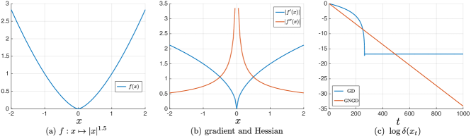
Figure 7: GD and GNGD on $f:x\mapsto|x|^{p}$, $p=1.5$.

Figure 7(a) shows the image of $f:x\mapsto|x|^{1.5}$. As shown in subfigure (b), the gradient of $f$ exists at $x=0$, and the Hessian $\left|f^{\prime\prime}(x)\right|\to\infty$ as $x\to 0$. The results of GD with $\eta=0.005$ and GNGD are presented in subfigure (c). The sub-optimality of GD update decreased for some time, and then it increased later. This is due to the Hessian is unbounded near $x=0$, and thus constant learning rates cannot guarantee monotonic progresses for GD. On the other hand, GNGD with $\eta=0.01$ enjoys $O(e^{-c\cdot t})$ convergence rate, verifying the results in the case (3) in Theorem 1.

F.2 $f:x\mapsto|x|^{p},$ $p>2$

As shown in Proposition 4, with $p\in(1,2)$, $f:x\mapsto|x|^{p}$ satisfies NŁ inequality with $\xi=1/p\in(0,1/2)$. As shown in Figure 8(a), the spectral radius of Hessian approaches $0$ as $x\to 0$, which is the case (1) in Theorem 1.

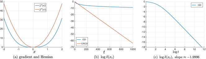
Figure 8: GD and GNGD on $f:x\mapsto|x|^{p}$, $p=4$.

Subfigure (c) shows that the standard GD with constant learning rate $\eta=0.01$ achieves sublinear rate about $O(1/t^{2})$, while subfigure (b) shows that GNGD with $\eta=0.01$ enjoys linear rate $O(e^{-c\cdot t})$, verifying Theorem 1.

F.3 Convergence Rates on GLM

Theorem 5 proves linear convergence rates $O(e^{-c\cdot t})$ for both GD and GNGD on GLM. We compare GD, NGD (Hazan et al., 2015), and GNGD on GLM, as shown in Figure 9.

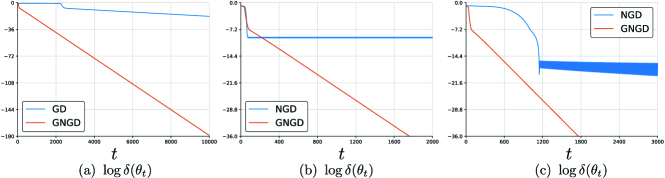
Figure 9: Convergence rates for GD, NGD, and GNGD on GLM.

Subfigure (a) presents the results of GD with $\eta=0.09$ and GNGD with $\eta=0.09$. Both GD and GNGD achieve linear $O(e^{-c\cdot t})$ rates, verifying Theorem 5. GD suffers from the plateaus at the early-stage optimization, which is consistent with Figure 1 and the explanations after Theorem 5. On the other hand, the slopes indicate that GNGD converges strictly faster than GD, which justifies the constant dependences ($C\geq C^{2}$) in Theorem 5. Subfigure (b) shows that standard NGD (Hazan et al., 2015) with constant learning rate $\eta=0.09$ does not converge. The NGD update keeps oscillating, which verifies our argument of using standard normalization for all $t\geq 1$ is not a good idea. Subfigure (c) presents the NGD using adaptive learning rate $\eta_{t}=\frac{0.09}{\sqrt{t}}$, which has faster convergence than NGD with constant $\eta$. However, GNGD still significantly outperforms NGD with $\eta_{t}=\frac{0.09}{\sqrt{t}}$, verifying the $O(e^{-c\cdot t})$ in Theorem 5 and $O(1/\sqrt{t})$ in Theorem 4.

F.4 Tree MDPs

Figure 10 shows the results for PG and GNPG beyond one-state MDPs. The environment is a synthetic tree with height $h$ and branching factor $b$. The total number of states is

$$S=\sum_{i=0}^{h-1}{b^{i}}.$$ (545)

The discount factor $\gamma=0.99$, and we set $\mu=\rho$ (e.g., in Algorithm 1 and Theorem 3), where $\rho(s_{0})=1$ for the root state $s_{0}$. For PG, in each iteration, we calculate the policy gradient (Lemma 15) to do one update. For GNPG, Algorithm 1 is used.

Subfigures (a) and (b) show the results for $h=b=4$, and $S=85$. The learning rate is $\eta=0.02$ for PG and GNPG. Subfigures (c) and (d) show the results for $h=5$ and $b=4$, and $S=341$. The learning rate is $\eta=0.05$ for PG and GNPG.

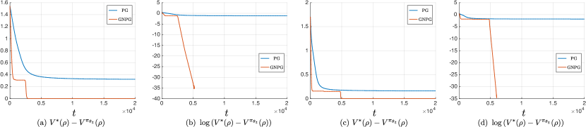
Figure 10: Results for PG and GNPG on tree MDPs. In (a) and (b), $S=85$. In (c) and (d), $S=341$.

References

- Agarwal et al. (2020) Agarwal, A., Kakade, S. M., Lee, J. D., and Mahajan, G. Optimality and approximation with policy gradient methods in markov decision processes. In Conference on Learning Theory, pp. 64–66. PMLR, 2020.
- Allen-Zhu et al. (2019) Allen-Zhu, Z., Li, Y., and Song, Z. A convergence theory for deep learning via over-parameterization. In International Conference on Machine Learning, pp. 242–252. PMLR, 2019.
- Bhandari & Russo (2020) Bhandari, J. and Russo, D. A note on the linear convergence of policy gradient methods. arXiv preprint arXiv:2007.11120, 2020.
- Bubeck (2014) Bubeck, S. Convex optimization: Algorithms and complexity. arXiv preprint arXiv:1405.4980, 2014.
- Cen et al. (2020) Cen, S., Cheng, C., Chen, Y., Wei, Y., and Chi, Y. Fast global convergence of natural policy gradient methods with entropy regularization. arXiv preprint arXiv:2007.06558, 2020.
- Cohen et al. (2021) Cohen, J., Kaur, S., Li, Y., Kolter, J. Z., and Talwalkar, A. Gradient descent on neural networks typically occurs at the edge of stability. In International Conference on Learning Representations, 2021.
- Hazan et al. (2015) Hazan, E., Levy, K., and Shalev-Shwartz, S. Beyond convexity: Stochastic quasi-convex optimization. Advances in neural information processing systems, 28:1594–1602, 2015.
- Hazan et al. (2019) Hazan, E., Kakade, S., Singh, K., and Van Soest, A. Provably efficient maximum entropy exploration. In International Conference on Machine Learning, pp. 2681–2691. PMLR, 2019.
- Kakade & Langford (2002) Kakade, S. and Langford, J. Approximately optimal approximate reinforcement learning. In ICML, volume 2, pp. 267–274, 2002.
- Karimi et al. (2016) Karimi, H., Nutini, J., and Schmidt, M. Linear convergence of gradient and proximal-gradient methods under the polyak-łojasiewicz condition. In Joint European Conference on Machine Learning and Knowledge Discovery in Databases, pp. 795–811. Springer, 2016.
- Kingma & Ba (2014) Kingma, D. P. and Ba, J. Adam: A method for stochastic optimization. arXiv preprint arXiv:1412.6980, 2014.
- Kurdyka (1998) Kurdyka, K. On gradients of functions definable in o-minimal structures. In Annales de l’institut Fourier, volume 48, pp. 769–783, 1998.
- Li et al. (2021) Li, G., Wei, Y., Chi, Y., Gu, Y., and Chen, Y. Softmax policy gradient methods can take exponential time to converge. arXiv preprint arXiv:2102.11270, 2021.
- Łojasiewicz (1963) Łojasiewicz, S. Une propriété topologique des sous-ensembles analytiques réels. Les équations aux dérivées partielles, 117:87–89, 1963.
- Mei et al. (2020a) Mei, J., Xiao, C., Dai, B., Li, L., Szepesvári, C., and Schuurmans, D. Escaping the gravitational pull of softmax. Advances in Neural Information Processing Systems, 33, 2020a.
- Mei et al. (2020b) Mei, J., Xiao, C., Szepesvari, C., and Schuurmans, D. On the global convergence rates of softmax policy gradient methods. In International Conference on Machine Learning, pp. 6820–6829. PMLR, 2020b.
- Nemirovski & Yudin (1983) Nemirovski, A. S. and Yudin, D. B. Problem complexity and method efficiency in optimization. 1983.
- Nesterov (2003) Nesterov, Y. Introductory lectures on convex optimization: A basic course, volume 87. Springer Science & Business Media, 2003.
- Polyak (1963) Polyak, B. T. Gradient methods for minimizing functionals. Zhurnal Vychislitel’noi Matematiki i Matematicheskoi Fiziki, 3(4):643–653, 1963.
- Sutton et al. (2000) Sutton, R. S., McAllester, D. A., Singh, S. P., and Mansour, Y. Policy gradient methods for reinforcement learning with function approximation. In Advances in neural information processing systems, pp. 1057–1063, 2000.
- Wilson et al. (2019) Wilson, A., Mackey, L., and Wibisono, A. Accelerating rescaled gradient descent: Fast optimization of smooth functions. arXiv preprint arXiv:1902.08825, 2019.
- Zhang et al. (2019) Zhang, J., He, T., Sra, S., and Jadbabaie, A. Why gradient clipping accelerates training: A theoretical justification for adaptivity. In International Conference on Learning Representations, 2019.