Causal Intervention for Leveraging Popularity Bias in Recommendation

Abstract.

Recommender system usually faces popularity bias issues: from the data perspective, items exhibit uneven (usually long-tail) distribution on the interaction frequency; from the method perspective, collaborative filtering methods are prone to amplify the bias by over-recommending popular items. It is undoubtedly critical to consider popularity bias in recommender systems, and existing work mainly eliminates the bias effect with propensity-based unbiased learning or causal embeddings. However, we argue that not all biases in the data are bad, i.e., some items demonstrate higher popularity because of their better intrinsic quality. Blindly pursuing unbiased learning may remove the beneficial patterns in the data, degrading the recommendation accuracy and user satisfaction.

This work studies an unexplored problem in recommendation — how to leverage popularity bias to improve the recommendation accuracy. The key lies in two aspects: how to remove the bad impact of popularity bias during training, and how to inject the desired popularity bias in the inference stage that generates top-$K$ recommendations. This questions the causal mechanism of the recommendation generation process. Along this line, we find that item popularity plays the role of confounder between the exposed items and the observed interactions, causing the bad effect of bias amplification. To achieve our goal, we propose a new training and inference paradigm for recommendation named Popularity-bias Deconfounding and Adjusting (PDA). It removes the confounding popularity bias in model training and adjusts the recommendation score with desired popularity bias via causal intervention. We demonstrate the new paradigm on the latent factor model and perform extensive experiments on three real-world datasets from Kwai, Douban, and Tencent. Empirical studies validate that the deconfounded training is helpful to discover user real interests and the inference adjustment with popularity bias could further improve the recommendation accuracy. We release our code at https://github.com/zyang1580/PDA.

1. Introduction

Recommender system provides personalized service for users to seek information, playing an increasingly important role in a wide range of online applications, such as e-commerce, news portal, content-sharing platform, and social media. However, the system faces popularity bias issues, which stand on the opposite of personalization. On one hand, the user-item interaction data usually exhibits long-tail distribution on item popularity — a few head items occupy most of the interactions whereas the majority of items receive relatively little attention (Mansoury et al., 2020; Abdollahpouri et al., 2017). On the other hand, the recommender model trained on such long-tail data not only inherits the bias, but also amplifies the bias, making the popular items dominate the top recommendations (Jannach et al., 2015; Abdollahpouri, 2020). Worse still, the feedback loop ecology of recommender system further intensifies such Matthew effect (Liu et al., 2019), causing notorious issues like echo chamber (Ge et al., 2020) and filter bubble (Steck, 2018). Therefore, it is essential to consider the popularity bias issue in recommender systems.

Existing work on popularity bias-aware recommendation mainly performs unbiased learning or ranking adjustment, which can be categorized into:

• Inverse Propensity Scoring (IPS), which adjusts the data distribution to be even by reweighting the interaction examples for model training (Schnabel et al., 2016; Gruson et al., 2019). Although IPS methods have sound theoretical foundations, they hardly work well in practice due to the difficulties in estimating propensities and high model variance.

• Causal Embedding, which uses bias-free uniform data to guide the model to learn unbiased embedding (Bonner and Vasile, 2018; Liu et al., 2020), forcing the model to discard item popularity. However, obtaining such uniform data needs to randomly expose items to users, which has the risk of hurting user experience. Thus the data is usually of a small scale, making the learning less stable.

• Ranking Adjustment, which performs post-hoc re-ranking on the recommendation list (Abdollahpouri et al., 2019; Zhu et al., 2021) or model regularization on the training (Abdollahpouri et al., 2017; Zhu et al., 2021). Both types of methods are heuristically designed to intentionally increase the scores of less popular items, which however lack theoretical foundations for effectiveness.

Instead of eliminating the effect of popularity bias, we argue that the recommender system should leverage the popularity bias. The consideration is that not all popularity biases in the data mean bad effect. For example, some items demonstrate higher popularity because of better intrinsic quality or representing current trends, which deserve more recommendations. Blindly eliminating the effect of popular bias will lose some important signals implied in the data, improperly suppressing the high-quality or fashionable items. Moreover, some platforms have the need of introducing desired bias into the system, e.g., promoting the items that have the potential to be popular in the future. This work aims to fill the research gap of effectively leveraging popularity bias to improve the recommendation accuracy.

To understand how item popularity affects the recommendation process, we resort to the language of causal graph (Pearl, 2009) for a qualitative analysis first. Figure 1(a) illustrates that traditional methods mainly perform user-item matching to predict the affinity score: $U$ (user node) and $I$ (item node) are the causes, and $C$ is the effect node to denote the interaction probability. An example is the prevalent latent factor model (Mnih and Salakhutdinov, 2007; He et al., 2020), which forms the prediction as the inner product between user embedding and item embedding. Since how a model forms the prediction implies how it assumes the labeled data be generated, this causal graph could also interpret the assumed generation process of the observed interaction data. Item popularity, although exerts a significant influence on data generation process, is not explicitly considered by such coarse-grained modeling methods.

We next consider how item popularity affects the process, enriching the causal graph to Figure 1(b). Let node $Z$ denote item popularity, which has two edges pointing to $C$ and $I$, respectively. First, $Z\rightarrow C$ means the item popularity directly affects the interaction probability, since many users have herd mentality (a.k.a., conformity), thus tend to follow the majority to consume popular items (Liu et al., 2016; Zheng et al., 2021). Second, $Z\rightarrow I$ means item popularity affects whether the item is exposed, since recommender system usually inherits the bias in the data and exposes popular items more frequently. Remarkably, we find $Z$ is the common cause for $I$ and $C$, acting as the confounder (Pearl, 2009) between the exposed items and the observed interactions. It means that, item popularity $Z$ affects the observed interaction data with two causal paths: 1) $Z\rightarrow C$ and 2) $Z\rightarrow I\rightarrow C$, wherein the second path contains the bad effect of bias amplification, since it increases observed interactions of popular items even though they may not well match user interest.

To remove the bad effect of popularity bias on model training, we need to intervene recommended items $I$ to make them immune to their popularity $Z$. Experimentally, it means we need to alter the exposure policy to make it free from the impact of item popularity and then recollect data, which is however costly and impossible to achieve for academia researchers. Thanks to the progress on causal science, we can achieve the same result with do-calculus (Pearl, 2009) without performing interventional experiments. In short, we estimate the user-item matching as $P(C|do(U,I))$ that cuts off the path $Z\rightarrow I$ during training, differing from the correlation $P(C|U,I)$ estimated by existing recommender models that confounds user interest with popularity bias. Through such deconfounded training, $P(C|do(U,I))$ estimates user interest matching on items more accurately than $P(C|U,I)$, removing the spurious correlations between $I$ and $C$ due to the confounder of $Z$. During the inference stage, we infer the ranking score as $P(C|do(U,I),do(Z))$, intervening the item popularity $Z$ with our desired bias (e.g., the forecasted popularity in the testing stage).

The main contributions of this work are summarized as follows:

• We analyze how popularity bias affects recommender system with causal graph, a powerful tool but is seldom used in the community; we identify that the bad impact of popularity bias stems from the confounding effect of item popularity.

• We propose Popularity-bias Deconfounding and Adjusting (PDA), a novel framework that performs deconfounded training with do-calculus and causally intervenes the popularity bias during recommendation inference.

• We conduct extensive experiments on three real datasets, validating the effectiveness of our causal analyses and methods.

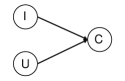
(a) Causal graph of traditional methods.

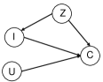
(b) Causal graph that considers item popularity.

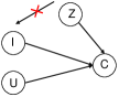
(c) We cut off $Z\rightarrow I$ for model training.

Figure 1. Causal graphs to describe the recommendation process. U: user, I: exposed item, C: interaction probability, Z: item popularity. We identify $Z$ as the confounder between $I$ and $C$, and propose deconfounded training with $P(C|do(U,I))$ as the interest matching.

2. Primary knowledge

We use uppercase character (e.g., $U$) to denote a random variable and lowercase character (e.g., $u$) to denote its specific value. We use characters in calligraphic font (e.g., $\mathcal{U}$) to represent the sample space of the corresponding random variable, and use $P(\cdot)$ to represent probability distribution of a random variable.

Let $\mathcal{D}$ denote the historical data, which is sequentially collected through $T$ stages, i.e., $\mathcal{D}=\{\mathcal{D}_{1}\cup\cdots\cup\mathcal{D}_{T}\}$; $\mathcal{U}=\{u_{1},\dots,u_{|\mathcal{U}|}\}$ and $\mathcal{I}=\{i_{1},\dots,i_{{|\mathcal{I}|}}\}$ denote all users and items, respectively. Through learning on historical data, the recommender system is expected to capture user preference and serves well for the next stage $T+1$. That is, it aims to obtain high recommendation accuracy on $\mathcal{D}_{T+1}$. In this work, we are interested in the factor of item popularity, defining the local popularity of item $i$ on the stage $t$ as:

(1) $$\small m_{i}^{t}=D_{i}^{t}/\sum_{j\in\mathcal{I}}D_{j}^{t},$$

where $D_{i}^{t}$ denotes the number of observed interactions for item $i$ in $\mathcal{D}_{t}$. We can similarly define the global popularity of an item $m_{i}$ based on its interaction frequency in $\mathcal{D}$, but we think the local popularity has a larger impact on the system’s exposure mechanism and user decision, since the system is usually periodically retrained and the most recent data has the largest impact.

Popularity drift.

Intuitively, item popularity is dynamic and changes over time, meaning that the impact of popularity bias could also be dynamic. To quantify the popularity drift, we define a metric named Drift of Popularity (DP) to measure the drift between two stages. First, we represent each stage $t$ as a probability distribution over items: $\big{[}m_{1}^{t},\dots,m_{|\mathcal{I}|}^{t}\big{]}$, where each entry denotes an item’s frequency in the stage. Then, we use the Jensen-Shannon Divergence (JSD) (Endres and Schindelin, 2003) to measure the similarity between two stages:

(2) $$DP(t,s)=JSD\left(\big{[}m_{1}^{t},\dots,m_{|\mathcal{I}|}^{t}\big{]},\big{[}m_{1}^{s},\dots,m_{|\mathcal{I}|}^{s}\big{]}\right),$$

where $t$ and $s$ are the two stages. Similar to JSD, the range of DP is $[0,log(2)]$, and a higher value indicates a larger popularity drift.

Figure 2(a) shows the DP value of two successive stages, i.e., $DP(t,t+1)$ where $t$ iterates from 1 to 9, on three real-world datasets (details in Section 4.1.1). We can see that the popularity drift obviously exists in all three datasets, and different datasets exhibit different levels of popularity drift. Figure 2(b) shows the DP value of the first and present stage, i.e., $DP(1,t)$, which measures the accumulated popularity drift. We can see a clear increasing trend, indicating that the longer the time interval is, the large popularity drift the data exhibits. These results reveal that popularity bias and its impact also change with time. The popularity bias in the future stage differs from that of past stages. If we set the target of model generalization as pursuing high accuracy on the next stage data $\mathcal{D}_{T+1}$, then a viable way is to predict popularity trend and inject it into the recommendations.

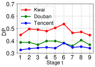
(a) $DP(t,t+1)$

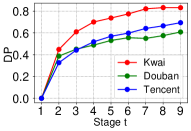
(b) $DP(1,t)$

Figure 2. Popularity drift between: (a) two successive stages $DP(t,t+1)$; (b) the first and present stage $DP(1,t)$.

3. Methodology

We first analyze the impact of item popularity on recommendation from a fundamental view of causality. Then we present our PDA framework that eliminates the bad effect of popularity bias on training and intervenes the inference stage with desired bias. Lastly, we present in-depth analyses of our method.

3.1. Causal View of Recommendation

Figure 1(b) shows the causal graph that accounts for item popularity in affecting recommendation. By definition, causal graph (Pearl, 2009) is a directed acyclic graph where a node denotes a variable and an edge denotes a causal relation between two nodes (Pearl, 2009). It is widely used to describe the process of data generation, which can guide the design of predictive models. Next, we explain the rationality of this causal graph.

• Node $U$ represents the user node, e.g., user profile or history feature that is used for representing a user.

• Node $I$ represents the item node. We assume a user can only interact with (e.g., click) the items that have been exposed to him/her, thus $I$ denotes the exposed item.

• Node $C$ represents the interaction label, indicating whether the user has chosen/consumed the exposed item.

• Node $Z$ represents the item popularity, which can be seen as a hidden variable since it is usually not explicitly modeled by traditional methods (e.g., (Mnih and Salakhutdinov, 2007; He et al., 2020) form predictions with Figure 1(a)). But it has a large impact on the recommendation.

• Edges $\{U,I,Z\}\rightarrow C$ denote that an interaction label $C$ is determined by the three factors: user $U$, item $I$, and the item’s popularity $Z$. Traditional methods only consider $\{U,I\}\rightarrow C$ which is easy to explain: the matching between user interest and item property determines whether a user consumes an item. Here we intentionally add a cause node $Z$ for capturing user conformity — many users have the herd mentality and tend to follow the majority to consume popular items (Liu et al., 2016; Zheng et al., 2021). Thus, whether there is an interaction is the combined effect of $U,I$ and $Z$.

• Edge $Z\rightarrow I$ denotes that item popularity affects the exposure of items. This phenomenon has been verified on many recommender models, which are shown to favor popular items after training on biased data (Abdollahpouri, 2020).

From this causal graph, we find that item popularity $Z$ is a confounder that affects both exposed items $I$ and observed interactions $C$. This results in two causal paths starting from $Z$ that affect the observed interactions: $Z\rightarrow C$ and $Z\rightarrow I\rightarrow C$. The first path is combined with user-item matching to capture the user conformity effect, which is as expected. In contrast, the second path means that item popularity increases the exposure likelihood of popular items, making the observed interactions consist of popular items more. Such effect causes bias amplification, which should be avoided since an authentic recommender model should estimate user preference reliably and is immune to the exposure mechanism.

In the above text, we have explained the causal graph from the view of data generation. In fact, it also makes sense to interpret it from the view of model prediction. Here, we denote $U$ and $I$ as user embedding and item embedding, respectively, and traditional models apply inner product (Mnih and Salakhutdinov, 2007; He et al., 2020) or neural network (He et al., 2017) above them for prediction (i.e., Figure 1(a)). Item popularity $Z$ is not explicitly considered in most models, however, it indeed affects the learning of item embedding. For example, it increases the vector length of popular items, making inner product models score popular items high for every user (Zheng et al., 2021). Such effect justifies the edge $Z\rightarrow I$, which exerts a negative impact to learn real user interest.

To sum up, regardless of which explanation for the causal graph, $Z\rightarrow I$ causes the bad effect and should be eliminated in formulating the predictive model.

3.2. Deconfounded Training

We now consider how to obtain a model that is immune to the impact of $Z\rightarrow I$. Intuitively, if we can intervene the exposure mechanism to make it randomly expose items to users, then the collected interaction data is free from the impact of $Z\rightarrow I$. Directly training traditional models on it will do. However, the feasibility and efficacy of such solutions are low: first, only the recommender builder can intervene the exposure mechanism, and anyone else (e.g., academia researcher) has no permission to do it; second, even for recommender builder that can intervene the exposure mechanism, they can only use small random traffic, since random exposure hurts user experience much. Effective usage of small uniform data remains an open problem in recommendation research (Bonner and Vasile, 2018; Liu et al., 2020).

Fortunately, the progress of causal science provides us a tool to achieve intervention without performing the interventional experiments (Pearl, 2009). The secret is the do-calculus. In our context, performing $do(I)$ forces to remove the impact of $I$’s parent nodes, achieving our target. As such, we formulate the predictive model as $P(C|do(U,I))$, rather than $P(C|U,I)$ estimated by traditional methods.

Let the causal graph shown in Figure 1(b) be $G$, and the intervened causal graph shown in Figure 1(c) be $G^{\prime}$. Then, performing do-calculus on $G$ leads to:

(3) $$\small\begin{split}P(C|do(U,I))&\overset{(1)}{=}P_{G^{\prime}}(C|U,I)\\ &\overset{(2)}{=}\sum_{z}P_{G^{\prime}}(C|U,I,z)P_{G^{\prime}}(z|U,I)\\ &\overset{(3)}{=}\sum_{z}P_{G^{\prime}}(C|U,I,z)P_{G^{\prime}}(z)\\ &\overset{(4)}{=}\sum_{z}P(C|U,I,z)P(z),\end{split}$$

where $P_{G^{\prime}}(\cdot)$ denotes the probability function evaluated on $G^{\prime}$. Below explains this derivation step by step:

• (1) is because of backdoor criterion (Pearl, 2009) as the only backdoor path $I\leftarrow Z\rightarrow C$ in $G$ has been blocked by $do(U,I)$;

• (2) is because of Bayes’ theorem;

• (3) is because that $U$ and $I$ are independent with $Z$ in $G^{\prime}$;

• (4) $P(C|U,I,Z)=P_{G^{\prime}}(C|U,I,Z)$ is because that the causal mechanism $\{U,I,Z\}\rightarrow C$ is not changed when cutting off $Z\rightarrow I$, $P(Z)=P_{G^{\prime}}(Z)$ since $Z$ has the same prior on the two graphs.

Next, we consider how to estimate $P(C|do(U,I))$ from data. Apparently, we need to first estimate $P(C|U,I,Z)$, and then estimate $\sum_{z}P(C|U,I,z)P(z)$.

Step 1. Estimating $P(C|U,I,Z)$. This conditional probability function evaluates that given a user-item pair $U=u,I=i$ and the item’s present popularity as $Z=m_{i}^{t}$, how likely the user will consume the item. Let the parameters of the conditional probability function be $\Theta$, we can follow traditional recommendation training to learn $\Theta$, for example, optimizing the pairwise BPR objective function on historical data $\mathcal{D}$:

(4) $$\small\max_{\Theta}\sum_{(u,i,j)\in\mathcal{D}}\text{log}\sigma\left(P_{\Theta}\left(c=1|u,i,m_{i}^{t}\right)-P_{\Theta}\left(c=1|u,j,m_{j}^{t}\right)\right),$$

where $j$ denotes the negative sample for $u$, $\sigma(\cdot)$ is the sigmoid function. The $L_{2}$ regularization is used but not shown for brevity.

Having established the learning framework, we next consider how to parameterize $P_{\Theta}(c=1|u,i,m_{i}^{t})$. Of course, one can design it as any differentiable model, factorization machines, or neural networks. But here our major consideration is to decouple the user-item matching with item popularity. The benefits are twofold: 1) decoupling makes our framework extendable to any collaborative filtering model that concerns user-item matching; and 2) decoupling enables fast adjusting of popularity bias in the inference stage (see Section 3.3), since we do not need to re-evaluate the whole model. To this end, we design it as:

(5) $$\small P_{\Theta}(c=1|u,i,m_{i}^{t})=ELU^{\prime}(f_{\Theta}(u,i))\times({m}_{i}^{t})^{\gamma},$$

where $f_{\Theta}(u,i)$ denotes any user-item matching model and we choose the simple Matrix Factorization (MF) in this work; hyper-parameter $\gamma$ is to smooth the item popularity and can control the strength of conformity effect: setting $\gamma=0$ means no impact and larger value assigns larger impact. $ELU^{\prime}(\cdot)$ is a variant of the Exponential Linear Unit (Clevert et al., 2016) activation function that ensures the positivity of the matching score:

(6) $$\small ELU^{\prime}(x)=\begin{cases}e^{x},&\text{if }x\leq 0\\ x+1,&\text{else}\end{cases}$$

This is to ensure the monotonicity of the probability function since $({m}_{i}^{t})^{\gamma}$ is always a positive number. Lastly, note that one needs to normalize $P_{\Theta}(c=1|u,i,m_{i}^{t})$ to make it a rigorous probability function, but we omit it since it is time-consuming and does not affect the ranking of items.

Step 2. Estimating $\sum_{z}P(C|U,I,z)P(z)$. Now we move forward to estimate the interventional probability $P(C|do(U,I))$. Since the space of $Z$ is large, it is inappropriate to sum over its space for each prediction evaluation. Fortunately, we can perform the following reduction to get rid of the sum:

$$\small\begin{split}P(C|do(U,I))&=\sum_{z}P(C|U,I,z)P(z)\\ &=\sum_{z}ELU^{\prime}(f_{\Theta}(u,i))\times z^{\gamma}P(z)\\ &=ELU^{\prime}(f_{\Theta}(u,i))\sum_{z}z^{\gamma}P(z)\\ &=ELU^{\prime}(f_{\Theta}(u,i))E(Z^{\gamma})\end{split}$$

where $E(Z^{\gamma})$ denotes the expectation of $Z^{\gamma}$. Note that the expectation of one variable is a constant. Since $P(C|do(U,I))$ is used to rank items for a user, the existence of $E(Z^{\gamma})$ does not change the ranking. We can thus use $ELU^{\prime}(f_{\Theta}(u,i))$ to estimate $P(C|do(U,I)$.

To summarize, we fit the historical interaction data with $P_{\Theta}(c=1|u,i,m_{i}^{t})$, and use the user-item matching component $ELU^{\prime}(f_{\Theta}(u,i))$ for deconfounded ranking. We name this method as Popularity-bias Deconfounding (PD).

3.3. Adjusting Popularity Bias in Inference

Owing to $P(C|do(U,I))$, we can eliminate the bad effect of popularity bias. We now seek for better usage of popularity bias, e.g., promoting the items that have the potential to be popular. Assume the target popularity bias is $\tilde{z}$, and we want to endow the recommendation policy with this bias. To achieve the target, we just need to do the intervention of $Z=\tilde{z}$ for model inference:

(7) $$\small P(C|do(U=u,I=i),do(Z=\tilde{z}))=P_{\Theta}(c=1|u,i,\tilde{m}_{i}),$$

where $\tilde{m}_{i}$ denotes the popularity value of $\tilde{z}$. This intervention probability directly equals the conditional probability since there is no backdoor path between $Z$ and $C$ in the causal graph. Since the focus of this work is not on popularity prediction, we employ a simple time series forecasting method to set $\tilde{m}_{i}$:

(8) $$\small\tilde{m}_{i}=m_{i}^{T}+\alpha(m_{i}^{T}-m_{i}^{T-1}),$$

where $m_{i}^{T}$ is the popularity value of the last stage, and $\alpha$ is the hyper-parameter to control the strength of popularity drift in predicting the future. We name this method as Popularity-bias Deconfounding and Adjusting (PDA).

Figure 3 illustrates the workflow of PDA where the training stage optimizes Equation (4) and the inference stage can adjust the popularity bias as:

(9) $$\small PDA_{ui}=ELU^{\prime}(f_{\Theta}(u,i))\times(\tilde{m}_{i})^{\tilde{\gamma}}.$$

$\tilde{\gamma}$ denotes the popularity smoothing hyper-parameter used for model inference, which can be different from that used in training. This is to consider that the strength of popularity bias can drift in the future. In practice, setting $\tilde{\gamma}=\gamma$ can achieve expected performance (cf. Table 2). Setting $\tilde{\gamma}=0$ degrades the method to PD that uses only interest matching for recommendation. Considering the importance of properly stopping model training, PDA uses a model selection strategy based on the adjusted recommendation, which is slightly different from that of PD (see Algorithm 1).

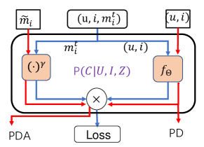
Figure 3. The workflow of our method. The blue arrows represent the training stage and the red arrows represent the inference stage.

3.4. Comparison with Correlation $P(C|U,I)$

In the beginning, we argue that traditional methods estimate the correlation $P(C|U,I)$ and suffer from the bad effect of popularity bias amplification. Here we analyze the difference between $P(C|U,I)$ and $P(C|do(U,I))$ to offer more insights on this point.

We first transform $P(C|U,I)$ with the following steps:

(10) $$\small\begin{split}P(C|U,I)&\overset{(1)}{=}\sum_{z}P(C,z|U,I)\\ &\overset{(2)}{=}\sum_{z}P(C|U,I,z)P(z|U,I)\\ &\overset{(3)}{=}\sum_{z}P(C|U,I,z)P(z|I)\\ &\overset{(4)}{\propto}\sum_{z}P(C|U,I,z)P(I|z)P(z)\end{split}$$

(1) is the definition of marginal distribution; (2) is because of the Bayes’ theorem; (3) is because $U$ is independent to $Z$ according to the causal graph; (4) is because of the Bayes’ theorem.

Comparing with $P(C|do(U,I))=\sum_{z}P(C|U,I,z)P(z)$, we can see that $P(C|U,I)$ has an additional term: $P(I|Z)$, which fundamentally changes the recommendation scoring. Suppose $I=i$ is a popular item, $P(C|U,I=i,Z=m_{i}^{t})$ is a large value since $m_{i}^{t}$ is large, which means the term has a large contribution to the prediction score. $P(I=i|Z=m_{i}^{t})$ is also a large value due to the popularity bias in the exposure mechanism. Multiplying the two terms further enlarges the score of $i$, which gives $i$ a higher score than it deserves. As a result, the popularity bias is improperly amplified. This comparison further justifies the rationality and necessity of $P(C|do(U,I))$ for learning user interests reliably.

Input: dataset $\mathcal{D}=\{(u,i,m_{i}^{t})\}$; hyper-parameter $\gamma$; predicted popularity $\{\tilde{m}_{i}\}$; mode: PD or PDA

1 while stop condition is not reached do

2       Update model parameters $\Theta$ by optimizing Equation (4);

3       if mode==PD then validate model with $ELU^{{}^{\prime}}(f_{\Theta}(u,i))$;

4       else validate model with Equation (9) (simplify $\tilde{\gamma}=\gamma$);

5      

6 end while

7if mode==PD then recommend items using $ELU^{{}^{\prime}}(f_{\Theta}(u,i))$;

8 else recommend items using Equation (9) (simplify $\tilde{\gamma}=\gamma$);

Algorithm 1 PD/PDA

4. Experiments

In this section, we conduct experiments to answer two main questions: RQ1: Does PD achieve the goal of removing the bad effect of popularity bias? How is its performance compared with existing methods? RQ2: Can PDA effectively inject desired popularity bias? To what extent leveraging popularity bias enhance the recommendation performance.

Table 1. Recommendation performance after deconfounded training on the three datasets. “RI” refers to the relative improvement of PD over the corresponding baseline. The best results are highlighted in bold and sub-optimal results are underlined.

Dataset	Methods	Top 20					Top 50
		Recall	Precision	HR	NDCG	RI	Recall	Precision	HR	NDCG	RI
Kwai	MostPop	0.0014	0.0019	0.0341	0.0030	632.4%	0.0040	0.0021	0.0802	0.0036	480.9%
	BPRMF	0.0054	0.0057	0.0943	0.0067	146.3%	0.0125	0.0053	0.1866	0.0089	121.0%
	xQuad	0.0054	0.0057	0.0948	0.0068	145.0%	0.0125	0.0053	0.1867	0.0090	120.3%
	BPR-PC	0.0070	0.0056	0.0992	0.0072	125.0%	0.0137	0.0046	0.1813	0.0092	123.7%
	DICE	0.0053	0.0056	0.0957	0.0067	147.8%	0.0130	0.0052	0.1872	0.0090	119.0%
	PD	0.0143	0.0138	0.2018	0.0177	-	0.0293	0.0118	0.3397	0.0218	-
Douban	MostPop	0.0218	0.0297	0.2373	0.0349	75.4%	0.0490	0.0256	0.3737	0.0406	55.9%
	BPRMF	0.0274	0.0336	0.2888	0.0405	47.0%	0.0581	0.0291	0.4280	0.0475	34.3%
	xQuad	0.0274	0.0336	0.2895	0.0391	48.3%	0.0581	0.0291	0.4281	0.0473	34.4%
	BPR-PC	0.0282	0.0307	0.2863	0.0381	51.6%	0.0582	0.0271	0.4260	0.0457	38.0%
	DICE	0.0273	0.0336	0.2845	0.0421	46.2%	0.0513	0.0273	0.4000	0.0460	44.5%
	PD	0.0453	0.0454	0.3970	0.0607	-	0.0843	0.0362	0.5271	0.0686	-
Tencent	MostPop	0.0145	0.0043	0.0684	0.0093	340.8%	0.0282	0.0035	0.1181	0.0135	345.8%
	BPRMF	0.0553	0.0153	0.2005	0.0328	27.1%	0.1130	0.0129	0.3303	0.0497	25.3%
	xQuad	0.0552	0.0153	0.2007	0.0326	27.3%	0.1130	0.0129	0.3302	0.0497	25.3%
	BPR-PC	0.0556	0.0153	0.2018	0.0331	26.5%	0.1141	0.0128	0.3322	0.0500	24.9%
	DICE	0.0516	0.0149	0.1948	0.0312	32.8%	0.1010	0.0132	0.3312	0.0486	29.0%
	PD	0.0715	0.0195	0.2421	0.0429	-	0.1436	0.0165	0.3875	0.0641	-

4.1. Experimental Settings

4.1.1. Datasets

We conduct experiments on three datasets:

1) Kwai: This dataset was adopted in Kuaishou User Interest Modeling Challenge, which contains click/like/follow records between users and videos. It spans about two weeks. In this paper, we only utilize clicking data. Following previous work (Wang et al., 2019a), we take 10-core filtering to make sure that each user and each item have at least 10 interacted records. After filtering, the experimented data has 7,658,510 interactions between 37,663 users and 128,879 items.

2) Douban Movie: This dataset is collected from a popular review website Douban in China by (Song et al., 2019). It contains user ratings for movies and spans more than ten years. We take all rating records as positive samples and only utilize the data after 2010. The 10-core filtering is also adopted. After filtering, there are 7,174,218 interactions between 47,890 users and 26,047 items.

3) Tencent: This dataset is collected from Tencent short-video platform from Dec 27 2020 to Jan 6 2021. In this dataset, user interactions are likes, which are reflective of user satisfaction but far more sparse than clicks. Because of its high sparsity, we adopt the 5-core filtering setting, obtaining 1,816,046 interactions between 80,339 users and 27,070 items.

Following Cañamares and Castells (2018), we split the datasets chronologically. In particular, we split the datasets into 10 time stages according to the interaction time, and each stage has the same time interval. The last stage is left for validation and testing, in which $30\%$ of users are regarded as validation set and the other $70\%$ of users are regarded as testing set. Note that we do not consider new users and new items in validation and testing.

4.1.2. Baselines

We compare PD with the following baselines:

- MostPop. This method simply recommends the most popular items for all users without considering personalization.

- BPRMF, which optimizes the MF model with BPR loss (Rendle et al., 2009).

- xQuAD (Abdollahpouri et al., 2019). This is a Ranking Adjustment method that aims to increase the coverage of long-tail items in the recommendation list. We use the codes released by the authors, and utilize it to re-rank the result of BPRMF. Following its original setting, we tune the bias controlling hyper-parameter $\lambda$ in $[0,1]$ with step 0.1.

- BPR-PC (Zhu et al., 2021). This is a state-of-the-art Ranking Adjustment method for controlling popularity bias. It has two choices: re-ranking and regularization. Here we implement the re-ranking method based on the BPRMF, because this method shows better performance in the original paper. Following the paper, we tune the bias controlling hyper-parameters $\alpha$ [0.1, 2.0] with step 0.2, and $\beta$ in [0, 1] with step 0.2.

- DICE (Zheng et al., 2021). This is a state-of-the-art method for learning causal embeddings to handle the popularity bias. It designs a framework with causality-oriented data to disentangle user interest and conformity into two sets of embedding. We use the codes provided by the authors, and we take the settings suggested for large datasets instead of the default settings since our datasets are relatively large. Because DICE demonstrates superior performance over IPS-based methods (Schnabel et al., 2016; Gruson et al., 2019), we do not include IPS-based methods as baselines.

To evaluate the effect of PDA on leveraging desired popularity bias, we compare it with the following popularity-aware methods:

- MostRecent (Ji et al., 2020). This is an improved version of MostPop, which recommends the most popular items in the last stage rather than in the entire history. Note that PDA takes the last stage to forecast the popularity of next stage to make adjustment.

- BPRMF(t)-pop (Nagatani and Sato, 2017). This method models the temporal popularity by training a set of time-specific parameters for each stage. We directly utilize the parameters corresponding to the last training stage for validation and testing.

- BPRMF-A and DICE-A. We enhance BPRMF and DICE to inject desired popularity bias during inference in the same manner as PDA by substituting $f_{\Theta}(u,i)$ with the prediction of BPRMF/DICE in Equation (9). We tune the smooth hyper-parameter $\tilde{\gamma}$.

4.1.3. Hyper-parameters and Metrics.

For a fair comparison, all methods are optimized by BPR loss and tuned on the validation data. We optimize all models with the Adam (Kingma and Ba, 2014) optimizer with batch size as $2,048$ and default choice of learning rate (i.e., 0.001) for all the experiments. We search $L_{2}$ regularization coefficients in the range of $\{0.01,0.001\dots,10^{-6},0\}$ for all models. We adopt the early stopping strategy that stops training if Recall@20 on the validation data does not increase for 100 epochs. For DICE, we use its provided stopping strategy and tune the threshold for stopping to make it comparable to our strategy. For PD and PDA, we search $\gamma$ in $[0.02,0.25]$ with a step size of $0.02$. For BPRMF-A and DICE-A, we search $\tilde{\gamma}$ from $0.02$ to $1$ with a step size of $0.02$ and stop searching if the evaluation results do not change for $3$ steps.

To measure the recommendation performance, we adopt four widely-used evaluation metrics: Hit Ratio (HR), Recall, Precision, which consider whether the relevant items are retrieved within the top-$K$ positions, and NDCG that measures the relative orders among positive and negative items in the top-$K$ list. All metrics are computed by the all-ranking protocol — all items that are not interacted by a user are the candidates. We report the results of $K=20$ and $K=50$ in our experiments.

4.2. Deconfounding Performance (RQ1)

In this section, we will first study the recommendation performance of our proposed algorithm PD. Then, we analyze its recommendation lists and showcase its rationality. At last, we study the necessity of computing item popularity at different stages in training (i.e., computing local popularity).

4.2.1. Overall Performance

Table 1 shows the comparison of top-$K$ recommendation performance. From the table we can find:

• The proposed PD achieves the best performance, and consistently outperforms all the baselines on all datasets. This verifies the effectiveness of PD, which is attributed to the deconfounded training to remove the bad effect of popularity bias. In addition, the superior performance of PD reflects the rationality of our causal analysis and the potential of do-calculus in mitigating the bias issue in recommendation.

• PD achieves different degrees of improvement on the three datasets. In particular, PD outperforms all baselines by at least $119\%$, $34\%$, and $24\%$ on Kwai, Douban, and Tencent, respectively. We think the difference in the improvement is due to the different properties of the three datasets. For example, the level of popularity drift in the data differs substantially as shown in Figure 2: the popularity drifts of Kwai are much larger than that of the other two datasets. Higher drifts imply that item popularity $Z$ has larger impact on the recommendation data. That is why the proposed PD outperforms baseline methods the most on the Kwai dataset. Hence, we believe that formulating the recommender model as $P(C|do(U,I))$ has larger advantages over $P(C|U,I)$ in the scenarios exhibiting higher popularity drift.

• For BPR-PC and xQuad, which perform ranking adjustment, only BPR-PC has limited improvements over BPRMF on recall, i.e., ranking adjustment has little effect in our setting. The reason is that: heuristic adjustment of the original model prediction can only guarantee an increase in the proportion of long-tail items but cannot guarantee the promoted items are of real interest. BPR-PC performs better than xQuad since xQuad only considers group-level popularity, while BPR-PC computes popularity in a finer granularity at item level.

• DICE tries to disentangle popularity and interest influence for an observed interaction to get causal embedding. It only demonstrates a similar performance to BPRMF in our setting, which indicates the rationality of leveraging popularity bias instead of blindly eliminating the bias. Note that in the original paper of DICE, the evaluation data is manually intervened to ensure an even distribution of testing interactions over items, which removes popularity bias in the testing data. Whereas in our setting, the evaluation data is split by time to reflect real-world evaluation of recommender system, and contains popularity bias. Although DICE boosts the scores of unpopular items over popular items, it may under-estimate users’ interest matching for popular items.

Table 2. Top-K recommendation performance with popularity adjusting on Kwai, Douban, and Tencent Datasets.

Datasets		Kwai				Douban				Tencent
		top 20		top 50		top 20		top 50		top 20		top 50
Methods		Recall	NDCG	Recall	NDCG	Recall	NDCG	Recall	NDCG	Recall	NDCG	Recall	NDCG
MostRecent		0.0074	0.0096	0.0139	0.011	0.0398	0.0582	0.0711	0.0615	0.0360	0.0222	0.0849	0.0359
BPRMF(t)-pop		0.0188	0.0241	0.0372	0.0286	0.0495	0.0682	0.0929	0.0760	0.1150	0.0726	0.2082	0.1001
	(a)	0.0191	0.0249	0.0372	0.0292	0.0482	0.0666	0.0898	0.0744	0.1021	0.0676	0.1805	0.0905
BPRMF-A	(b)	0.0201	0.0265	0.0387	0.0306	0.0486	0.0667	0.0901	0.0746	0.1072	0.0719	0.1886	0.0953
	(a)	0.0242	0.0315	0.0454	0.0363	0.0494	0.0681	0.0890	0.0736	0.1227	0.0807	0.2161	0.1081
DICE-A	(b)	0.0245	0.0323	0.0462	0.0370	0.0494	0.0680	0.0882	0.0734	0.1249	0.0839	0.2209	0.1116
	(a)	0.0279	0.0352	0.0531	0.0413	0.0564	0.0746	0.1066	0.0845	0.1357	0.0873	0.2378	0.1173
PDA	(b)	0.0288	0.0364	0.0540	0.0429	0.0565	0.0745	0.1066	0.0843	0.1398	0.0912	0.2418	0.1210

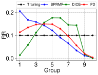
(a) Kwai

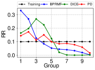
(b) Douban

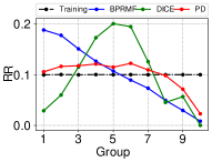
(c) Tencent

(d) std. dev.

Figure 4. Recommendation rate(RR) over item groups.

4.2.2. Recommendation Analysis

We claim that PD can alleviate the amplification of popularity bias, i.e., removing the bad effect of popularity bias. We conduct an analysis of the recommendation lists to show that deconfounded recommendation does not favor popular items as much as conventional recommendations. Items are placed into $10$ different groups in two steps: (1) we sort items according to their popularity in descending order and (2) we divide the items into $10$ groups and ensure that the sum of popularity over items in each group is the same. As such, the number of items will increase from group 1 to group 10 and the average popularity among items in each group decreases from group 1 to group 10. Hence we say group 1 is the most popular group and group 10 is the least popular group.

For each method, we sum the number of times of items recommended from each group. Then we divide this number by the total number of recommendations to get the recommendation rate for each group. Formally, we define recommendation rate (RR) for group $g$ as:

$$\small RR(g,algo)=\frac{\sum_{i\in Group_{g}}{RC(i,algo)}}{\sum_{i\in AllGroups}{RC(i,algo)}}$$

where $RC(i,algo)$ gives the number of times the algorithm $algo$ recommends item $i$ in top-$K$ recommendation lists.

For training, the recommendation rate of different groups is uniform (see the black line in Figure 4). If more popular groups have higher recommendation rates, there is the amplification of popularity bias. We show the recommendation rates of each group by different methods in Figure 4, in which (a), (b), and (c) are the results on Kwai, Douban, and Tencent, respectively. Figure 4 (d) is to show the standard deviation (std. dev.) of recommendation rates over all the groups: a smaller value means the recommendation rate is more uniform and is closer to the recommendation rates from training set. The main findings are as follows.

• It is clear that popularity bias will be amplified by BPRMF. Figures 4 (a) (b) (c) show that as the average item popularity decreases from group 1 to group 10, the recommendation rate decreases almost linearly. The gap between the chances to recommend popular items and unpopular items becomes bigger in the recommendation lists compared with that in the training set.

• For DICE, the recommendation rate increases initially and then decreases from group 1 to group 10. This is because DICE strategically increases the scores of unpopular items to suppress the problem of amplified interest for popular items. However, this suppression brings two side effects: (1) the items from group 1 and group 2 are over-suppressed such that they have lower chances to be recommended than they have in the training set on Kwai and Tencent and (2) it over-amplifies the interest for the middle groups that contain sub-popular items. As such, blindly eliminating popularity bias would remove the beneficial patterns in the data.

• In Figure 4 (a) (b) (c), the RRs of PD exhibit lines that are flatter than other methods, which are the most similar to the training set. Moreover, as we can see in Figure 4 (d), the RR of PD has the smallest standard deviation across groups, indicating the least difference across groups. These results verify that PD provides relatively fair recommendations across groups, and will not over-amplify or over-suppress interest for popular items. Along with the recommendation performance in Table 1, the results demonstrate the rationality and effectiveness of only removing the bad effect of popularity bias by deconfounded training.

• For the group $10$, which has the least popular items, PD has a little higher recommendation rate than other methods. However, PD also cannot provide enough chances of recommendation because of the sparse interactions of items in this group and the insufficient learning of item embedding.

Note that we omit the RRs of the ranking adjustment methods (i.e., BPR-PC and xQuad) since their recommendation rates for unpopular items are manually increased. Instead of tuning the recommendation rate for groups of different popularity, we concentrate more on whether the learned embedding can precisely reveal the real interests of users.

4.2.3. Global Popularity V.S. Local Popularity.

To investigate the necessity of local popularity, we evaluate a variant of PD that uses global popularity defined on the interaction frequency in the entire training set $\mathcal{D}$. We keep the other settings the same as PD and name this method as PD-Global (PD-G). Figure 5 shows the recommendation performance of PD and PD-G on the three datasets. Due to the limited space, we only show the results on recall and NDCG for top-$50$ recommendation, other metrics show the similar results. According to the figure, PD-G is far worse than PD, which verifies the importance of calculating item popularity locally. We believe PD-G performs poorly because there is only one instance of $P(C|u,i,Z)$ on $Z$, making $P(C|u,i,Z)$ hard to be learned well.

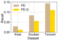
(a) Recall

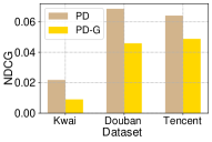
(b) NDCG

Figure 5. Comparisons between PD and PD-G on Recall@50 and NDCG@50. PD-G is a version of PD that computes item popularity over the total training set.

4.3. Performance of Adjusting Popularity (RQ2)

In this section, we verify the performance of our proposed method PDA, which introduces some desired popularity bias into recommendation. Firstly, we compare our method with the baselines that inject some popularity bias as well — MostRecent, BPRMF (t)-pop, BPRMF-A, and DICE-A. Secondly, we study the influence of refined prediction of item popularity for PDA. Lastly, we demonstrate overall improvements compared with the baseline model BPRMF.

4.3.1. Comparisons with Baselines.

We utilize two methods to predict the popularity of the testing stage. Specially, method (a) takes the popularity of items from the last stage $\mathcal{D}_{T}$ as the predicted popularity, while method (b) computes populairity as Equation (8). We apply both (a) and (b) to PDA, DICE-A, and BPRMF-A. The results are shown in Table 2, which lead to the following observations:

• By comparing the results of PDA, DICE-A, BPRMF-A, and MostRecent with the results of PD, DICE, BPRMF, and MostPop in Table 1, we find that introducing desired popularity bias into recommendations can improve the recommendation performance. This validates the rationality of leveraging popularity bias, i.e., promoting the items that have the potential to be popular (desired popularity bias) benefits recommendation performance.

• Compared with other methods, PDA can outperform both the method BPRMF(t)-pop, which is specially designed for utilizing temporal popularity, and the modified methods BPRMF-A and DICE-A. This is attributed to PDA introducing the desired popularity bias by an intervention, preventing the learning model to amplify the effect of popularity and injecting desired popularity bias in inference, whereas other models are influenced by popularity bias in training. The results validate the advantage of causal intervention in more accurately estimating true interests.

• On Kwai and Tencent, method (b) outperforms method (a), indicating that introducing the linear predicted popularity is more effective than straightforwardly utilizing the popularity from the previous stage; On Douban, these two methods achieve almost the same performance. This is because the Douban dataset spans over a longer period of time than the other two datasets, making it harder to predict the popularity from the trends of popularity in training stages.

Figure 6. PDA recommendation performance regarding Recall@50 and NDCG@50 on Kwai and Douban, with the last training stage split into $N$ sub-stages.

4.3.2. More Refined Predictions for Popularity.

We conduct an experiment to show that the performance of PDA can be improved with more refined predicted popularity. To get more refined predictions, we uniformly split the data in the last training stage into $N$ sub-stages by time, and achieve a more refined prediction of popularity in the last sub-stage, which is closest to the testing stage. We set $N=1,2,4,8,16$ and employ method (a) to predict the desired popularity. The results are shown in Figure 6. The performance of PDA can be improved with better-predicted popularity for testing. On the Kwai dataset, the performance first increases and then slightly decreases as $N$ increases. However, on the Douban dataset, with a larger $N$, the performance does not drop evidently. This is mainly because the item space of Kwai is far larger than Douban, but they have a similar number of interactions. When $N$ is set to a large value, the interaction frequency is insufficient to accurately compute item popularity for Kwai. This experiment shows that the performance of PDA can be further improved with a more precise prediction of popularity.

4.3.3. Total Improvements of PDA

To quantify the strengths of PDA, we show the relative improvements of PDA over the basic model that PDA is built on, i.e., BPRMF in Table 3. On the Kwai dataset, we get more than $241\%$ improvements over all metrics. On the Douban and Tencent datasets, for the recall and NDCG, we get at least $97\%$ improvements, and for precision and HR, we get at least $57\%$ improvements. The results clearly indicate the superiority of PDA in recommendation and the huge potential of causal analysis and inference for leveraging bias in recommendation.

5. Related Works

This work is closely related to two topics: popularity bias in recommender system and causal recommendation.

Table 3. The total relative improvements of PDA compared with the base recommendation model, i.e., BPRMF. Each result is averaged on top 20 and top 50.

Dataset	Recall	Precision	HR	NDCG
Kwai	488%	441%	241%	532%
Douban	124%	68%	57%	97%
Tencent	133%	133%	79%	161%

5.1. Popularity Bias

Popularity bias has long been recognized as an important issue in recommendation systems. One line of research (Abdollahpouri et al., 2020; Jannach et al., 2015; Cañamares and Castells, 2018; Mansoury et al., 2020; Steck, 2011) studies the phenomenon of popularity bias. (Jannach et al., 2015) studies how popularity bias influences different recommendation models and concludes that popularity has a larger impact on BPR-based models (Zheng et al., 2021) than point-wise models (He et al., 2017); (Abdollahpouri et al., 2020) tries to study the relation between popularity bias and other problems such as fairness and calibration. Another line of research (Zheng et al., 2021; Zhu et al., 2021; Abdollahpouri et al., 2019, 2017; Abdollahpouri, 2020; Schnabel et al., 2016; Bonner and Vasile, 2018) attempts to improve recommendation performance by removing popularity bias. These works mainly consider three types of methods: IPS-based methods (Schnabel et al., 2016; Gruson et al., 2019), causal embedding-based methods (Bonner and Vasile, 2018; Liu et al., 2020; Zheng et al., 2021), and the methods based on post-hoc re-ranking or model regularization (Zhu et al., 2021; Abdollahpouri et al., 2019, 2017; Kamishima et al., 2014; Oh et al., 2011). Similar to our work, a very recent work (Zheng et al., 2021) also tries to compute the influence of popularity via causal approaches. The difference is that we analyze the causal relations from a confounding perspective whearas this important aspect was not considered in their work. Some other works have attempted to remove the impact of other bias problems (Chen et al., 2020), position bias (Agarwal et al., 2019), selection bias (Wang et al., 2019b), and exposure bias (Liang et al., 2016; Chen et al., 2018) etc. The most widely considered method for handling aforementioned biases is IPS-based method (Schnabel et al., 2016; Zhu et al., 2020; Ai et al., 2018; Zhang et al., 2020). However, there is no guaranteed accuracy for estimating propensity scores. Utilizing unbiased data is another option for solving bias problems (Bonner and Vasile, 2018; Liu et al., 2020), however the unbiased data is difficult to obtain and may hurt user experience (Wang et al., 2019b).

Some other methods recognize the importance of utilizing popularity and consider drifted popularity to improve the model performance (Nagatani and Sato, 2017; Ji et al., 2020; Lex et al., 2020; Anelli et al., 2019). (Lex et al., 2020) tries to utilize temporal popularity in music recommendation and (Jonnalagedda et al., 2016) utilizes local popularity for recommending news. (Nagatani and Sato, 2017; Anelli et al., 2019; Ji et al., 2020) also try to utilize temporal popularity for general recommendation. The biggest difference between our work and other works is that we precisely differentiate popularity bias to be removed and popularity drift to be taken advantage of.

5.2. Causal Recommendation

Some efforts have considered causality in recommendation. The first type of work is on confounding effects (Wang et al., 2020b; Sato et al., 2020; Chaney et al., 2018; Christakopoulou et al., 2020). For example, (Wang et al., 2020b) takes the de-confounding technique in linear models to learn real interest influenced by unobserved confounders. They learn substitutes for unobserved confounders by fitting exposure data. (Sato et al., 2020) tries to estimate the causal effect of the recommending operation. They consider the features of users and items as confounders, and reweight training samples to solve the confounding problem. (Chaney et al., 2018) explores the impact of algorithmic confounding on simulated recommender systems. (Christakopoulou et al., 2020) identifies expose rate as a confounder for user satisfaction estimation and uses IPS to handle the confounding problem. In this work, we introduce a different type of confounder that is brought by item popularity.

The second type is counterfactual learning methods (Mehrotra et al., 2020; Yuan et al., 2019; Wang et al., 2020a). (Mehrotra et al., 2020) utilizes a quasi-experimental Bayesian framework to quantify the effect of treatments on an outcome to generate counterfactual data, where counterfactual data refers to the outcomes of unobserved treatments. (Yuan et al., 2019) utilizes a model that is learned with few unbiased data to generate labels for unobserved data. (Wang et al., 2020a) extends Information Bottleneck (Wang et al., 2020a) to counterfactual learning with the idea that the counterfactual world should be as informative as the factual world to deal with the Missing-Not-At-Random problem (Wang et al., 2019b). Though these works study the problem of causal recommendation, they do not specifically consider popularity bias as well as popularity drift for boosting recommendation performance.

6. conclusion

In this work, we study how to model and leverage popularity bias in recommender system. By analyzing the recommendation generation process with the causal graph, we find that item popularity is a confounder that misleads the estimation of $P(C|U,I)$ as done by traditional recommendation models. Different from existing work that eliminates popularity bias, we point out that some popularity bias should be decoupled for better usage. We propose a Popularity-bias Deconfounding and Adjusting framework to deconfound and leverage popularity bias for better recommendation. We conduct experiments on three real-world datasets, providing insightful analyses on the rationality of PDA.

This work showcased the limitation of pure data-driven models for recommendation, despite their dominant role in recommendation research and industry. We express the prior knowledge of how the data is generated for recommendation training as a causal graph, performing deconfounded training and intervened inference based on the causal graph. We believe this new paradigm is general for addressing the bias issues in recommendation and search systems, and will extend its impact to jointly consider more factors, such as position bias and selection bias. Moreover, we are interested in extending our method to the state-of-the-art graph-based recommendation models and incorporate the content features of users and items.

- (1)
- Abdollahpouri (2020) Himan Abdollahpouri. 2020. Popularity Bias in Recommendation: A Multi-stakeholder Perspective. Ph.D. Dissertation. University of Colorado.
- Abdollahpouri et al. (2017) Himan Abdollahpouri, Robin Burke, and Bamshad Mobasher. 2017. Controlling Popularity Bias in Learning-to-Rank Recommendation. In Proceedings of the Eleventh ACM Conference on Recommender Systems. 42–46.
- Abdollahpouri et al. (2019) Himan Abdollahpouri, Robin Burke, and Bamshad Mobasher. 2019. Managing Popularity Bias in Recommender Systems with Personalized Re-ranking. In Proceedings of the Thirty-Second International Florida Artificial Intelligence Research Society Conference. 413–418.
- Abdollahpouri et al. (2020) Himan Abdollahpouri, Masoud Mansoury, Robin Burke, and Bamshad Mobasher. 2020. The Connection Between Popularity Bias, Calibration, and Fairness in Recommendation. In Fourteenth ACM Conference on Recommender Systems. 726–731.
- Agarwal et al. (2019) Aman Agarwal, Ivan Zaitsev, Xuanhui Wang, Cheng Li, Marc Najork, and Thorsten Joachims. 2019. Estimating Position Bias without Intrusive Interventions. In Proceedings of the Twelfth ACM International Conference on Web Search and Data Mining. 474–482.
- Ai et al. (2018) Qingyao Ai, Keping Bi, Cheng Luo, Jiafeng Guo, and W Bruce Croft. 2018. Unbiased Learning to Rank with Unbiased Propensity Estimation. In The 41st International ACM SIGIR Conference on Research & Development in Information Retrieval. 385–394.
- Anelli et al. (2019) Vito Walter Anelli, Tommaso Di Noia, Eugenio Di Sciascio, Azzurra Ragone, and Joseph Trotta. 2019. Local Popularity and Time in Top-N Recommendation. In European Conference on Information Retrieval. 861–868.
- Bonner and Vasile (2018) Stephen Bonner and Flavian Vasile. 2018. Causal Embeddings for Recommendation. In Proceedings of the 12th ACM conference on recommender systems. 104–112.
- Cañamares and Castells (2018) Rocío Cañamares and Pablo Castells. 2018. Should I Follow the Crowd? A Probabilistic Analysis of the Effectiveness of Popularity in Recommender Systems. In The 41st International ACM SIGIR Conference on Research & Development in Information Retrieval. 415–424.
- Chaney et al. (2018) Allison JB Chaney, Brandon M Stewart, and Barbara E Engelhardt. 2018. How Algorithmic Confounding in Recommendation Systems Increases Homogeneity and Decreases Utility. In Proceedings of the 12th ACM Conference on Recommender Systems. 224–232.
- Chen et al. (2020) Jiawei Chen, Hande Dong, Xiang Wang, Fuli Feng, Meng Wang, and Xiangnan He. 2020. Bias and Debias in Recommender System: A Survey and Future Directions. arXiv preprint arXiv:2010.03240 (2020).
- Chen et al. (2018) Jiawei Chen, Yan Feng, Martin Ester, Sheng Zhou, Chun Chen, and Can Wang. 2018. Modeling Users’ Exposure with Social Knowledge Influence and Consumption Influence for Recommendation. In Proceedings of the 27th ACM International Conference on Information and Knowledge Management. 953–962.
- Christakopoulou et al. (2020) Konstantina Christakopoulou, Madeleine Traverse, Trevor Potter, Emma Marriott, Daniel Li, Chris Haulk, Ed H Chi, and Minmin Chen. 2020. Deconfounding User Satisfaction Estimation from Response Rate Bias. In Fourteenth ACM Conference on Recommender Systems. 450–455.
- Clevert et al. (2016) Djork-Arné Clevert, Thomas Unterthiner, and Sepp Hochreiter. 2016. Fast and Accurate Deep Network Learning by Exponential Linear Units (ELUs). In 4th International Conference on Learning Representations.
- Endres and Schindelin (2003) Dominik Maria Endres and Johannes E Schindelin. 2003. A New Metric for Probability Distributions. IEEE Transactions on Information Theory 49, 7 (2003), 1858–1860.
- Ge et al. (2020) Yingqiang Ge, Shuya Zhao, Honglu Zhou, Changhua Pei, Fei Sun, Wenwu Ou, and Yongfeng Zhang. 2020. Understanding Echo Chambers in E-commerce Eecommender Systems. In Proceedings of the 43rd International ACM SIGIR Conference on Research and Development in Information Retrieval. 2261–2270.
- Gruson et al. (2019) Alois Gruson, Praveen Chandar, Christophe Charbuillet, James McInerney, Samantha Hansen, Damien Tardieu, and Ben Carterette. 2019. Offline Evaluation to Make Decisions about Playlist Recommendation Algorithms. In Proceedings of the Twelfth ACM International Conference on Web Search and Data Mining. 420–428.
- He et al. (2020) Xiangnan He, Kuan Deng, Xiang Wang, Yan Li, Yongdong Zhang, and Meng Wang. 2020. Lightgcn: Simplifying and Powering Graph Convolution Network for Recommendation. In Proceedings of the 43rd International ACM SIGIR Conference on Research and Development in Information Retrieval. 639–648.
- He et al. (2017) Xiangnan He, Lizi Liao, Hanwang Zhang, Liqiang Nie, Xia Hu, and Tat-Seng Chua. 2017. Neural Collaborative Filtering. In Proceedings of the 26th International Conference on World Wide Web. 173–182.
- Jannach et al. (2015) Dietmar Jannach, Lukas Lerche, Iman Kamehkhosh, and Michael Jugovac. 2015. What Recommenders Recommend: an Analysis of Recommendation Biases and Possible Countermeasures. User Modeling and User-Adapted Interaction (2015), 427–491.
- Ji et al. (2020) Yitong Ji, Aixin Sun, Jie Zhang, and Chenliang Li. 2020. A Re-visit of the Popularity Baseline in Recommender Systems. In Proceedings of the 43rd International ACM SIGIR Conference on Research and Development in Information Retrieval. 1749–1752.
- Jonnalagedda et al. (2016) Nirmal Jonnalagedda, Susan Gauch, Kevin Labille, and Sultan Alfarhood. 2016. Incorporating Popularity in a Personalized News Recommender System. PeerJ Computer Science 2 (2016), e63.
- Kamishima et al. (2014) Toshihiro Kamishima, Shotaro Akaho, Hideki Asoh, and Jun Sakuma. 2014. Correcting Popularity Bias by Enhancing Recommendation Neutrality. In Poster Proceedings of the 8th ACM Conference on Recommender Systems.
- Kingma and Ba (2014) Diederik P Kingma and Jimmy Ba. 2014. Adam: A Method for Stochastic Optimization. arXiv preprint arXiv:1412.6980 (2014).
- Lex et al. (2020) Elisabeth Lex, Dominik Kowald, and Markus Schedl. 2020. Modeling Popularity and Temporal Drift of Music Genre Preferences. Transactions of the International Society for Music Information Retrieval 3, 1 (2020).
- Liang et al. (2016) Dawen Liang, Laurent Charlin, James McInerney, and David M Blei. 2016. Modeling user exposure in recommendation. In Proceedings of the 25th International Conference on World Wide Web. 951–961.
- Liu et al. (2020) Dugang Liu, Pengxiang Cheng, Zhenhua Dong, Xiuqiang He, Weike Pan, and Zhong Ming. 2020. A General Knowledge Distillation Framework for Counterfactual Recommendation via Uniform Data. In Proceedings of the 43rd International ACM SIGIR Conference on Research and Development in Information Retrieval. 831–840.
- Liu et al. (2016) Yiming Liu, Xuezhi Cao, and Yong Yu. 2016. Are You Influenced by Others When Rating? Improve Rating Prediction by Conformity Modeling. In Proceedings of the 10th ACM Conference on Recommender Systems. 269–272.
- Liu et al. (2019) Yudan Liu, Kaikai Ge, Xu Zhang, and Leyu Lin. 2019. Real-Time Attention Based Look-Alike Model for Recommender System. In Proceedings of the 25th ACM SIGKDD International Conference on Knowledge Discovery & Data Mining. 2765–2773.
- Mansoury et al. (2020) Masoud Mansoury, Himan Abdollahpouri, Mykola Pechenizkiy, Bamshad Mobasher, and Robin Burke. 2020. Feedback Loop and Bias Amplification in Recommender Systems. In Proceedings of the 29th ACM International Conference on Information & Knowledge Management. 2145–2148.
- Mehrotra et al. (2020) Rishabh Mehrotra, Prasanta Bhattacharya, and Mounia Lalmas. 2020. Inferring the Causal Impact of New Track Releases on Music Recommendation Platforms through Counterfactual Predictions. In Fourteenth ACM Conference on Recommender Systems. 687–691.
- Mnih and Salakhutdinov (2007) Andriy Mnih and Russ R Salakhutdinov. 2007. Probabilistic Matrix Factorization. In Advances in neural information processing systems, Vol. 20. 1257–1264.
- Nagatani and Sato (2017) Koki Nagatani and Masahiro Sato. 2017. Accurate and Diverse Recommendation based on Users’ Tendencies toward Temporal Item Popularity. In Proceedings of the 1st Workshop on Temporal Reasoning in Recommender Systems co-located with 11th ACM Conference on Recommender Systems. 35–39.
- Oh et al. (2011) Jinoh Oh, Sun Park, Hwanjo Yu, Min Song, and Seung-Taek Park. 2011. Novel Recommendation Based on Personal Popularity Tendency. In 2011 IEEE 11th International Conference on Data Mining. 507–516.
- Pearl (2009) Judea Pearl. 2009. Causality. Cambridge University Press.
- Rendle et al. (2009) Steffen Rendle, Christoph Freudenthaler, Zeno Gantner, and Lars Schmidt-Thieme. 2009. BPR: Bayesian Personalized Ranking from Implicit Feedback. In Proceedings of the Twenty-Fifth Conference on Uncertainty in Artificial Intelligence. 452–461.
- Sato et al. (2020) Masahiro Sato, Sho Takemori, Janmajay Singh, and Tomoko Ohkuma. 2020. Unbiased Learning for the Causal Effect of Recommendation. In Fourteenth ACM Conference on Recommender Systems. 378–387.
- Schnabel et al. (2016) Tobias Schnabel, Adith Swaminathan, Ashudeep Singh, Navin Chandak, and Thorsten Joachims. 2016. Recommendations as Treatments: Debiasing Learning and Evaluation. In Proceedings of the 33nd International Conference on Machine Learning. 1670–1679.
- Song et al. (2019) Weiping Song, Zhiping Xiao, Yifan Wang, Laurent Charlin, Ming Zhang, and Jian Tang. 2019. Session-Based Social Recommendation via Dynamic Graph Attention Networks. In Proceedings of the Twelfth ACM International Conference on Web Search and Data Mining. ACM, 555–563.
- Steck (2011) Harald Steck. 2011. Item Popularity and Recommendation Accuracy. In Proceedings of the Fifth ACM Conference on Recommender Systems. 125–132.
- Steck (2018) Harald Steck. 2018. Calibrated Recommendations. In Proceedings of the 12th ACM Conference on Recommender Systems. 154–162.
- Wang et al. (2019a) Xiang Wang, Xiangnan He, Meng Wang, Fuli Feng, and Tat-Seng Chua. 2019a. Neural Graph Collaborative Filtering. In Proceedings of the 42nd international ACM SIGIR conference on Research and development in Information Retrieval. 165–174.
- Wang et al. (2019b) Xiaojie Wang, Rui Zhang, Yu Sun, and Jianzhong Qi. 2019b. Doubly Robust Joint Learning for Recommendation on Data Missing Not at Random. In Proceedings of the 36th International Conference on Machine Learning. 6638–6647.
- Wang et al. (2020b) Yixin Wang, Dawen Liang, Laurent Charlin, and David M. Blei. 2020b. Causal Inference for Recommender Systems. In Fourteenth ACM Conference on Recommender Systems. 426–431.
- Wang et al. (2020a) Zifeng Wang, Xi Chen, Rui Wen, Shao-Lun Huang, Ercan E. Kuruoglu, and Yefeng Zheng. 2020a. Information Theoretic Counterfactual Learning from Missing-Not-At-Random Feedback. In Advances in Neural Information Processing Systems 33: Annual Conference on Neural Information Processing Systems 2020.
- Yuan et al. (2019) Bowen Yuan, Jui-Yang Hsia, Meng-Yuan Yang, Hong Zhu, Chih-Yao Chang, Zhenhua Dong, and Chih-Jen Lin. 2019. Improving Ad Click Prediction by Considering Non-displayed Events. In Proceedings of the 28th ACM International Conference on Information and Knowledge Management. 329–338.
- Zhang et al. (2020) Wenhao Zhang, Wentian Bao, Xiao-Yang Liu, Keping Yang, Quan Lin, Hong Wen, and Ramin Ramezani. 2020. Large-scale Causal Approaches to Debiasing Post-click Conversion Rate Estimation with Multi-task Learning. In Proceedings of The Web Conference 2020. 2775–2781.
- Zheng et al. (2021) Yu Zheng, Chen Gao, Xiang Li, Xiangnan He, Depeng Jin, and Yong Li. 2021. Disentangling User Interest and Conformity Bias for Recommendation with Causal Embedding. In Proceedings of the Web Conference 2021.
- Zhu et al. (2020) Ziwei Zhu, Yun He, Yin Zhang, and James Caverlee. 2020. Unbiased Implicit Recommendation and Propensity Estimation via Combinational Joint Learning. In Fourteenth ACM Conference on Recommender Systems. 551–556.
- Zhu et al. (2021) Ziwei Zhu, Yun He, Xing Zhao, Yin Zhang, Jianling Wang, and James Caverlee. 2021. Popularity-Opportunity Bias in Collaborative Filtering. In Proceedings of the 14th ACM International Conference on Web Search and Data Mining. 85–93.