Topological error correction with a Gaussian cluster state

Abstract

Topological error correction provides an effective method to correct errors in quantum computation. It allows quantum computation to be implemented with higher error threshold and high tolerating loss rates. We present a topological a error correction scheme with continuous variables based on an eight-partite Gaussian cluster state. We show that topological quantum correlation between two modes can be protected against a single quadrature phase displacement error occurring on any mode and some of two errors occurring on two modes. More interestingly, some cases of errors occurring on three modes can also be recognised and corrected, which is different from the topological error correction with discrete variables. We show that the final error rate after correction can be further reduced if the modes are subjected to identical errors occurring on all modes with equal probability. The presented results provide a feasible scheme for topological error correction with continuous variables and it can be experimentally demonstrated with a Gaussian cluster state.

I INTRODUCTION

Quantum computation (QC) can solve many complex problems more efficiently than classical computer Nielsen2000 . The measurement-based one-way QC provides a practical model to perform the universal QC based on the cluster states with different structures Raussendorf2001 ; Menicucci2006 . Quantum logic gates are realized by measurement and feedforward of measurement results based on the prepared cluster states in the measurement-based one-way QC Raussendorf2001 ; Menicucci2006 . However, during the QC, loss and noise may inevitably lead to errors in the computation results. Many quantum error correction (QEC) schemes have been experimentally demonstrated attempting to solve this problem Aoki2009 ; Lassen2010 ; Lassen2013 ; Hao . However, most fault-tolerant QCs with a high threshold error rate are difficult to implement in practice Knill ; Aliferis .

It has been shown that, cluster states whenever the underlying interaction graph can be embedded in a three-dimensional cell structure, the so-called cell complex Hatcher , can be used for QEC and fault-tolerant QC Fowler ; Raussendorf ; Stern . With a large cell complex, the quantum algorithms can be realized by suitable braiding-like manipulation of the defects Fowler . It is based on the property that some topological quantum correlations hold on defect-enclosing closed surfaces. We can use the redundancy of the cell complex to protect the topological correlations against local errors Raussendorf . By using the topological properties of the cluster states, we can realize the topological QC and the active topological error correction (TEC) at the same time Fowler ; Raussendorf ; Stern . This topological QC will lead to a higher error threshold Wang ; Raussendorf2007 and high tolerating loss rates Barrett in the scalable QC.

So far, there are many experimental explorations about the topological properties in a small topological quantum code unit. The anyonic fractional statistics have been demonstrated in different physical systems, such as photonic the system Chao-Yang ; Liu , the superconducting quantum circuit Zhong ; Song , the ultracold atom system Han-Ning , and nuclear magnetic resonance systems Feng ; Guilu . The anyons can serve as the fundamental units for a fault-tolerant QC. The TEC has been experimentally demonstrated using a simpler eight-photon graph state Yao2012 , where the quantum correlation is protected against a single local $Z$ error. This TEC method can significantly reduce the error rate.

Continuous variable (CV) QC, where information is encoded in the amplitude and phase quadratures of photonic harmonic oscillators, can be realized deterministically and unconditionally Menicucci2006 ; RMP1 ; RMP2 . The CV cluster state is a basic resource for one-way CV QC Menicucci2006 and quantum networks Wangyu ; Su2020 . Recently, large-scale CV cluster states in time the domain Andersen2019 ; Furusawa2019 and with frequency comb Olivier2014 ; Cai2017 have been prepared experimentally, and provide sufficient quantum resources for one-way CV QC. Several basic quantum logic operations Wang2010 ; Ukai2011 ; Ukai20112  and even a gate sequence Su2013 have been experimentally demonstrated in CV QC. What is more, several feasible schemes for the quantum cubic phase gate have been proposed Kevin ; Kazunori , which indicates that the full set of the basic operations will soon be obtained.

In the regime of CV QEC, according to the no-go theorem for Gaussian QEC that Gaussian errors cannot be corrected by using only Gaussian resources Niset ; Vuillot , the linear oscillator codes Vuillot ; Braunstein1998 are not suitable to correct generic Gaussian errors, while the code introduced by Gottesman, Kitaev, and Preskill (GKP code) Gottesman , toric GKP code Vuillot and the non-Gaussian oscillator-into-oscillators code Noh2019 can correct generic Gaussian errors. However, stochastic errors in CV QEC, which frequently occur in channels with environment fluctuations for example, can easily cause displacements and any other errors decomposable into displacements (including non-Gaussian errors) Loock2010 . In the stochastic error model, the input state described by the Wigner function $W_{in}$ is transformed into a state $W_{error}$ with probability $\gamma$, and it remains unchanged with probability $1-\gamma$ Loock2010 . Thus the output state is given by ${W}_{out}(x,p)=(1-\gamma){W}_{in}(x,p)+\gamma{W}_{error}(x,p)$. Note that even in the case that $W_{in}$ and $W_{error}$ are two Gassian states, the output state $W_{out}$ is no longer Gaussian. Thus, this error model describes a certain, simple form of non-Gaussian errors and it can be corrected by Gaussian states and Gaussian operations. Some CV QEC schemes against displacement errors have been experimentally demonstrated, for example, the nine-wave-packet code Aoki2009 , the five-wave-packet code Hao and the correcting code with the correlated noisy channels Lassen2013 . In addition, some basic concepts related to CV topological QC have been proposed in recent years, such as the CV anyon statistics Zhang2008 , the graphical calculus for CV states Menicucci2011 , the CV topological codes Tomoyuki and its application in quantum communication Menicucci2018 , the CV QC with anyons Darran , the exploration of CV fault-tolerant QC Menicucci2014 ; Lund , and topological entanglement entropy Tomoyuki2014 . These works established the foundation for the further research of CV topological QC. However, there has been no concrete scheme for CV TEC up to now.

In this paper, we propose a concrete scheme for CV TEC based on an eight-partite CV cluster state. At first, we propose the preparation scheme for a topological eight-partite CV cluster state, which is obtained by coupling eight squeezed states on a special beam-splitter network, and then we present the CV TEC scheme. We show that, within the abilities of the current technique, the quantum correlation can be protected against a single quadrature phase displacement error occurring on any modes. Moreover, some of the identical phase displacement errors occurring on two or three modes at the same time can also be recognized and corrected. This shows that the final error rate can be further reduced when we consider the phase sign of the syndrome results. The presented results are an essential step in CV TEC and are useful for further application in fault-tolerant CV QC.

The paper is organized as follows. In Sec. II, we present the preparation scheme for the topological eight-partite CV cluster state. In Sec. III, we show the details of the CV TEC scheme for a single mode error including the details of error recognition and error correction procedures. In section IV, we analyze the error rate of the presented CV TEC scheme. Finally, we present the discussion and conclusion in Sec. V.

II THE TOPOLOGICAL CV CLUSTER STATE

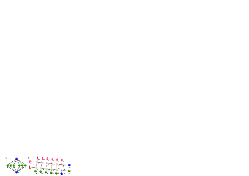
Figure 1: (a) The graph structure of the topological eight-partite CV cluster state. The connected lines represent the interaction between the neighbor nodes. Each node stands for an optical mode. (b) The beam-splitter network for the preparation of the cluster state. The ellipsoids represent the input squeezing states. The spheres represent the output cluster states. Circles including $i$ are Fourier transforms and $-1$ is a $180^{\circ}$ rotation in phase space.

Similar to the discrete variable systems, the CV analog of the Pauli operators are the Weyl–Heisenberg group of phase-space displacements. In detail, the relationships between them are $X\rightarrow\hat{X}(t)=e^{-it\hat{p}}$ and $Z\rightarrow\hat{Z}(s)=e^{is\hat{x}}$, where the amplitude ($\hat{x}$) and phase ($\hat{p}$) quadratures of an optical mode $\hat{a}$ are defined as $\hat{x}=(\hat{a}+\hat{a}^{\dagger})/2$ and $\hat{p}=(\hat{a}-\hat{a}^{\dagger})/2i$. The eight-partite CV cluster state for the CV TEC is described by a graph structure, as shown in the Fig. 1 (a). The CV cluster state is defined as Zhang2006 ; Menicucci2011

$$\hat{p}_{a}-\sum_{b\in N_{a}}\hat{x}_{b}\equiv\hat{\delta}_{a}\rightarrow 0,\ \ a\in G.$$ (1)

In the limit of infinite squeezing, the linear combinations of the quadrature components (so-called nullifiers) in Eq. (1) tend to zero. The modes $a\in G$ denote the vertices of the graph $G$, while the modes $b\in N_{a}$ are the nearest neighbors of mode $\hat{a}$. The CV cluster state can be generated with offline squeezing states and an appropriate beam-splitter network vanLoock2007 ; Su2007 ; Mitsuyoshi ; Su2012 .

The topological cluster state can be prepared by implementing an appropriate unitary transformation $U$ on a series of $\hat{p}$-squeezed input states, $\hat{a}_{l}=e^{+r}\hat{x}_{l}^{(0)}+ie^{-r}\hat{p}_{l}^{(0)}$, where $r$ is the squeezing parameter, $l=1,...,8,$and $\hat{x}^{(0)}$ and $\hat{p}^{(0)}$ represent the quadratures of a vacuum state whose variance is $\left\langle\Delta^{2}\hat{x}^{(0)}\right\rangle=\left\langle\Delta^{2}\hat{p}^{(0)}\right\rangle=1/4$, which corresponds to the shot-noise-level (SNL). Then, the output modes can be obtained by $\hat{C}_{k}=\sum\nolimits_{l}U_{kl}\hat{a}_{l}$. According to the method of building a Gaussian cluster state by linear optics vanLoock2007 , the transformation matrix $U$ should satisfy the condition $I$Im$U=A$Re$U$, where $I$ is the identity matrix and $A$ is the adjacency matrix of the graph $G$. Based on the unitarity of matrix $U$, we obtain Re$U($Re$U)^{T}=(I+A^{2})^{-1}$. We need $n(n-1)/2$ auxiliary conditions to get the matrix $U$. To make the matrix $U$ simple, we choose the auxiliary conditions to make more elements of $U$ to be zero according to symmetry of $A$. Finally, we get a simple form of $U$ as follows

$$\left(\begin{array}[]{cccccccc}\sqrt{\frac{3}{5}}&\frac{2}{\sqrt{35}}&\frac{2}{3\sqrt{7}}&\frac{-i}{\sqrt{91}}&\frac{2}{3\sqrt{11}}&\frac{i}{\sqrt{7}}&\frac{2}{\sqrt{143}}&0\\ 0&\frac{-5}{\sqrt{35}}&\frac{2}{3\sqrt{7}}&\frac{-i}{\sqrt{91}}&\frac{2}{3\sqrt{11}}&\frac{i}{\sqrt{7}}&\frac{2}{\sqrt{143}}&0\\ 0&0&\frac{-\sqrt{7}}{3}&\frac{-i}{\sqrt{91}}&\frac{2}{3\sqrt{11}}&\frac{i}{\sqrt{7}}&\frac{2}{\sqrt{143}}&0\\ 0&0&0&\frac{-i}{\sqrt{91}}&0&\frac{i}{\sqrt{7}}&\frac{-11}{\sqrt{143}}&0\\ 0&0&0&\frac{-i}{\sqrt{91}}&\frac{-3}{\sqrt{11}}&\frac{i}{\sqrt{7}}&\frac{2}{\sqrt{143}}&0\\ \frac{-2}{\sqrt{15}}&\frac{2}{\sqrt{35}}&\frac{2}{3\sqrt{7}}&\frac{-i}{\sqrt{91}}&\frac{2}{3\sqrt{11}}&\frac{i}{\sqrt{7}}&\frac{2}{\sqrt{143}}&\frac{1}{\sqrt{3}}\\ \frac{i}{\sqrt{15}}&\frac{-i}{\sqrt{35}}&\frac{-i}{3\sqrt{7}}&\frac{-7}{\sqrt{91}}&\frac{-i}{3\sqrt{11}}&0&\frac{-i}{\sqrt{143}}&\frac{i}{\sqrt{3}}\\ \frac{i}{\sqrt{15}}&\frac{-i}{\sqrt{35}}&\frac{-i}{3\sqrt{7}}&\frac{6}{\sqrt{91}}&\frac{-i}{3\sqrt{11}}&\frac{1}{\sqrt{7}}&\frac{-i}{\sqrt{143}}&\frac{i}{\sqrt{3}}\end{array}\right).$$ (2)

Generally, we can decompose an arbitrary $n\times n$ matrix $U$ into an at most $n(n+1)/2$ beam-splitter network Michael . Here, we decompose it symmetrically in order to use beam-splitters as little as possible. The decomposed matrix is $U=I_{2}(-1)\ F_{3}\ F_{4}$ $F_{5}$ $I_{6}(-1)$ $F_{7}$ $F_{8}$ $B_{68}^{+}(T_{12})$ $B_{78}^{+}(T_{11})$ $B_{16}^{+}(T_{10})$ $B_{17}^{+}(T_{9})$ $B_{26}^{+}(T_{8})$ $F_{6}$ $B_{27}^{+}(T_{7})$ $B_{36}^{+}(T_{6})$ $F_{3}$ $B_{37}^{-}(T_{5})$ $B_{56}^{-}(T_{4})$ $F_{5}$ $B_{57}^{-}(T_{3})$ $B_{46}^{-}(T_{2})$ $F_{4}$ $B_{47}^{+}(T_{1})$ $F_{4}$. In detail, $F_{k}$ denotes the Fourier transformation of mode $k$, which corresponds to a 90^∘ rotation in the phase space; $B_{kl}^{\pm}(T_{j})$ stands for the linearly optical transformation on the $j$-th beam-splitter with the transmittance of $T_{j}$ ($j=1,2,\ldots 12$), where $(B_{kl}^{\pm})_{kk}=\sqrt{T}$, $(B_{kl}^{\pm})_{kl}=\sqrt{1-T}$, $(B_{kl}^{\pm})_{lk}=\pm\sqrt{1-T}$, and $(B_{kl}^{\pm})_{ll}=\mp\sqrt{T}$ are elements of the beam-splitter matrix; and $I_{k}(-1)=e^{i\pi}$ corresponds to a 180^∘ rotation of mode $k$ in the phase space. The transmittances of the 12 beam-splitters are chosen as $T_{1}=1/78,T_{2}=6/7,T_{3}=54/55,T_{4}=5/6,T_{5}=35/36,T_{6}=4/5,T_{7}=20/21,T_{8}=3/4,T_{9}=9/10,T_{10}=2/3,T_{11}=2/3,$ and $T_{12}=1/2$, respectively. The beam-splitter network is shown in Fig. 1 (b).

The eight output modes $\hat{C}_{k}$ ($k=1,2,\ldots 8$) constitute the topological eight-partite cluster state. For the input states with finite-squeezing, the nullifiers of the cluster state are

$$\begin{array}[]{l}\hat{\delta}_{1}=\hat{p}_{1}-(\hat{x}_{7}+\hat{x}_{8})=e^{-r}\frac{\sqrt{5}\hat{p}_{1}^{(0)}+2\hat{p}_{8}^{(0)}}{\sqrt{3}},\\ \delta_{2}=\hat{p}_{2}-(\hat{x}_{7}+\hat{x}_{8})=e^{-r}(\frac{2\hat{p}_{1}^{(0)}}{\sqrt{15}}-\sqrt{\frac{7}{5}}\hat{p}_{2}^{(0)}+\frac{2\hat{p}_{8}^{(0)}}{\sqrt{3}}),\\ \hat{\delta}_{3}=\hat{p}_{3}-(\hat{x}_{7}+\hat{x}_{8})=e^{-r}(\frac{2\hat{p}_{1}^{(0)}}{\sqrt{15}}-\frac{2\hat{p}_{2}^{(0)}}{\sqrt{35}}-\frac{3\hat{p}_{3}^{(0)}}{\sqrt{7}}+\frac{2\hat{p}_{8}^{(0)}}{\sqrt{3}}),\\ \hat{\delta}_{4}=\hat{p}_{4}-(\hat{x}_{7}+\hat{x}_{8})\\ \ \ \ =e^{-r}(\frac{2\hat{p}_{1}^{(0)}}{\sqrt{15}}-\frac{2\hat{p}_{2}^{(0)}}{\sqrt{35}}-\frac{2\hat{p}_{3}^{(0)}}{3\sqrt{7}}-\frac{2\hat{p}_{5}^{(0)}}{3\sqrt{11}}-\frac{\sqrt{13}\hat{p}_{7}^{(0)}}{\sqrt{11}}+\frac{2\hat{p}_{8}^{(0)}}{\sqrt{3}}),\\ \hat{\delta}_{5}=\hat{p}_{5}-(\hat{x}_{7}+\hat{x}_{8})\\ \ \ \ =e^{-r}(\frac{2\hat{p}_{1}^{(0)}}{\sqrt{15}}-\frac{2\hat{p}_{2}^{(0)}}{\sqrt{35}}-\frac{2\hat{p}_{3}^{(0)}}{3\sqrt{7}}-\frac{\sqrt{11}\hat{p}_{5}^{(0)}}{3}+\frac{2\hat{p}_{8}^{(0)}}{\sqrt{3}}),\\ \hat{\delta}_{6}=\hat{p}_{6}-(\hat{x}_{7}+\hat{x}_{8})=\sqrt{3}e^{-r}\hat{p}_{8}^{(0)},\\ \hat{\delta}_{7}=\hat{p}_{7}-(\hat{x}_{1}+\hat{x}_{2}+\hat{x}_{3}+\hat{x}_{4}+\hat{x}_{5}+\hat{x}_{6})\\ \ \ \ =e^{-r}\frac{6\hat{p}_{6}^{(0)}-\sqrt{13}\hat{p}_{4}^{(0)}}{\sqrt{7}},\\ \hat{\delta}_{8}=\hat{p}_{8}-(\hat{x}_{1}+\hat{x}_{2}+\hat{x}_{3}+\hat{x}_{4}+\hat{x}_{5}+\hat{x}_{6})=\sqrt{7}e^{-r}\hat{p}_{6}^{(0)},\end{array}$$ (3)

respectively. In the case of infinite squeezing ($r\rightarrow\infty$), these nullifiers trend to zero, which satisfies the definition of the CV cluster state in Eq. (1).

III TOPOLOGICAL ERROR CORRECTION

For a given cluster state, its nullifiers can be used as the generators of the stabilizer operators for a topological code (a stabilizer QEC code) Tomoyuki . The topological quantum correlations in the qubit system are defined as $\mathbf{C}_{F}\equiv\langle\otimes_{f\in F}X_{f}\rangle=1$ Yao2012 . According to the corresponding relationship between the qubit Pauli operation with discrete variables and the single-mode Weyl$-$Heisenberg operation in the CV system, the single-mode Weyl$-$Heisenberg operator is described as $\hat{X}_{f}(t_{f})=e^{-it_{f}\hat{p}_{f}}(f=1,2,....,6)$ in the CV system, where $t_{f}$ is equal to $(-1)^{f}t$ Zhang2008 . By substituting the single-mode Weyl$-$Heisenberg operator into the topological quantum correlation in the qubit system, the definition of the topological quantum correlation in the CV system becomes $\mathbf{C}_{F}^{CV}\equiv\langle\otimes_{f\in F}\hat{X}_{f}[(-1)^{f}t]\rangle=\langle\otimes_{f\in F}e^{-i(-1)^{f}t\hat{p}_{f}}\rangle=1$. In CV system, it is convenient to use the nullifiers to analyze the protected quantum correlations when displacement errors occurred. So we have $\langle\sum_{f\in F}(-1)^{f}\hat{p}_{f}\rangle=0$ for the topological quantum correlations in the CV cluster state. For the prepared eight-partite the CV cluster state, the topological quantum correlations that can be protected are

$$\begin{array}[]{l}\hat{p}_{1}-\hat{p}_{2}=e^{-r}(\sqrt{\frac{3}{5}}\hat{p}_{1}^{(0)}+\sqrt{\frac{7}{5}}\hat{p}_{2}^{(0)}),\\ \hat{p}_{2}-\hat{p}_{5}=\frac{e^{-r}}{21}(-3\sqrt{35}\hat{p}_{2}^{(0)}+2\sqrt{7}\hat{p}_{3}^{(0)}+7\sqrt{11}\hat{p}_{5}^{(0)}),\\ \hat{p}_{3}-\hat{p}_{6}=e^{-r}(\frac{2}{\sqrt{15}}\hat{p}_{1}^{(0)}-\frac{2}{\sqrt{35}}\hat{p}_{2}^{(0)}-\frac{3}{\sqrt{7}}\hat{p}_{3}^{(0)}-\frac{1}{\sqrt{3}}\hat{p}_{8}^{(0)}),\\ \hat{p}_{4}-\hat{p}_{3}=\frac{e^{-r}}{33}(11\sqrt{7}\hat{p}_{3}^{(0)}-2\sqrt{11}\hat{p}_{5}^{(0)}-3\sqrt{143}\hat{p}_{7}^{(0)}),\\ \hat{p}_{5}-\hat{p}_{6}=e^{-r}(\frac{2\hat{p}_{1}^{(0)}}{\sqrt{15}}-\frac{2\hat{p}_{2}^{(0)}}{\sqrt{35}}-\frac{2\sqrt{7}\hat{p}_{3}^{(0)}}{21}-\frac{7\sqrt{11}\hat{p}_{5}^{(0)}}{21}-\frac{7\sqrt{3}\hat{p}_{8}^{(0)}}{21}),\end{array}$$ (4)

respectively. The corresponding variances of the topological quantum correalations are given by

$$\begin{array}[]{l}\left\langle\Delta^{2}(\hat{p}_{1}-\hat{p}_{2})\right\rangle=\frac{1}{2}e^{-2r},\\ \left\langle\Delta^{2}(\hat{p}_{2}-\hat{p}_{5})\right\rangle=\frac{1}{2}e^{-2r},\\ \left\langle\Delta^{2}(\hat{p}_{3}-\hat{p}_{6})\right\rangle=\frac{1}{2}e^{-2r},\\ \left\langle\Delta^{2}(\hat{p}_{4}-\hat{p}_{3})\right\rangle=\frac{1}{2}e^{-2r},\\ \left\langle\Delta^{2}(\hat{p}_{5}-\hat{p}_{6})\right\rangle=\frac{1}{2}e^{-2r},\end{array}$$ (5)

respectively. Obviously, in the ideal case of infinite squeezing ($r\rightarrow\infty$), these excess noises will vanish and the better the squeezing, the smaller the noise terms are.

At first, we analyze the CV TEC for a single phase displacement error in the ideal case, i.e. in the case of infinite squeezing. In the error correction procedure, any one of the above topological quantum correlations can be protected with the other four ”redundant” topological correlations as error syndromes in the TEC. In the process of error recognition, we choose any one of these five topological quantum correlations as the one needed to be protected and the other four as the auxiliary quantum correlations to get the error syndrome. Here, we take the quantum correlation $\hat{p}_{5}-\hat{p}_{6}$ as an example to analyze the TEC process. Figure 2 shows the circuit for error syndrome recognition in the case of an error that occurred on the mode $\hat{C}_{5}$. We use the homodyne detection systems to measure the quantum correlation of phase quadratures of the optical modes $\hat{C}_{1}$ to $\hat{C}_{6}$, respectively. The circuits for measuring the error syndrome can be realized by controlling the phase difference between the local light and the measured mode to get the phase quadrature ($\hat{p}$) and making an appropriate combination of the measured phase quadratures according to Eq. (4) to obtain the topological correlations of $\hat{p}_{1}-\hat{p}_{2}$, $\hat{p}_{2}-\hat{p}_{5}$, $\hat{p}_{3}-\hat{p}_{6}$, and $\hat{p}_{4}-\hat{p}_{3}$, respectively. If an error occurs on any mode, the quantum correlations that contain this mode will be affected at the same time. For example, when an error occurs on mode $\hat{C}_{5}$, the topological quantum correlation of $\hat{p}_{2}-\hat{p}_{5}$ will not be zero anymore. So, we can locate the position of the error based on the error syndromes of the auxiliary quantum correlations. Then, by feedforward of the measurement results of $\hat{p}_{2}-\hat{p}_{5}$ to $\hat{p}_{5}-\hat{p}_{6}$, the effect of error on $\hat{p}_{5}-\hat{p}_{6}$ will be corrected.

Table 1 shows the error syndrome results for all kinds of different single errors on modes $\hat{C}_{1}$ to $\hat{C}_{6}$ in the ideal case. If the error $\varepsilon$ doesn’t affect the syndrome correlation, the measured correlation will remain unchanged. Otherwise, the measured syndrome correlations will contain the nonzero error signal $\varepsilon$. The error syndrome results are different from each other when the error occurs on different modes. Comparing the measured results for the corresponding quantum correlations $\hat{p}_{1}-\hat{p}_{2},$ $\hat{p}_{2}-\hat{p}_{5},$ $\hat{p}_{3}-\hat{p}_{6},$and $\hat{p}_{4}-\hat{p}_{3}$ with the predictions in Table I, we can identify the position of error.

TABLE I.  Error syndrome with a single error mode.
Error mode	$\hat{p}_{1}-\hat{p}_{2}$	$\hat{p}_{2}-\hat{p}_{5}$	$\hat{p}_{3}-\hat{p}_{6}$	$\hat{p}_{4}-\hat{p}_{3}$	Requirement
1	$\varepsilon$	$0$	$0$	$0$	N
2	$-\varepsilon$	$\varepsilon$	$0$	$0$	N
3	$0$	$0$	$\varepsilon$	$-\varepsilon$	N
4	$0$	$0$	$0$	$\varepsilon$	N
5	$0$	$-\varepsilon$	$0$	$0$	Y
6	$0$	$0$	$-\varepsilon$	$0$	Y

After the position of error is confirmed, we can correct the error to eliminate the affection of error on the protected correlation according to the requirement. The correction requirements are summarized in Table I, where the symbol N stands for no need to correct the error and the symbol Y stands for the cases that need to correct the error. When the error occurs on the modes $\hat{C}_{1}$, $\hat{C}_{2},$ $\hat{C}_{3},$ and $\hat{C}_{4}$ respectively, the protected quantum correlation $\hat{p}_{5}-\hat{p}_{6}$ will not be affected by the error. So we do not need to correct the error. When an error $\varepsilon$ occurs on the mode $\hat{C}_{5},$ the correlation becomes $\hat{p}_{5}-\hat{p}_{6}\rightarrow\varepsilon$. To protect the correlation, we can make an addition of the detected term $\hat{p}_{2}-\hat{p}_{5},$ which tends to $-\varepsilon$, with $\hat{p}_{5}-\hat{p}_{6}$. We have $\hat{p}_{5}-\hat{p}_{6}+(\hat{p}_{2}-\hat{p}_{5})\rightarrow 0$ in the ideal case. So, the error influence is eliminated in this way. The error for mode $\hat{C}_{6}$ can be corrected similarly by subtracting the detected term $\hat{p}_{3}-\hat{p}_{6}$ from $\hat{p}_{5}-\hat{p}_{6}$. We have $\hat{p}_{5}-\hat{p}_{6}-(\hat{p}_{3}-\hat{p}_{6})\rightarrow 0.$

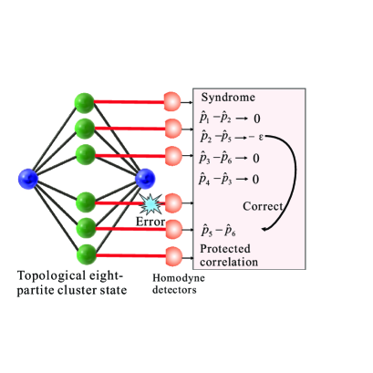
Figure 2: The circuit for error syndrome recognition and correction for the CV TEC. Here, we take the case of an error that occurs on mode $\hat{C}_{5}$ as an example.

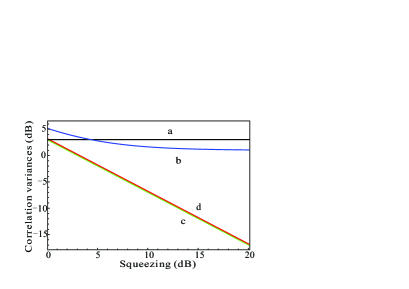
Figure 3: The dependence of the quantum correlation of $\hat{p}_{5}-\hat{p}_{6}$ on the squeezing of the initial squeezed states for different cases. Curve a is the corresponding shot-noise level for the protected correlation. Curve b is the correlation variance when no correction is used. Curve c is the correlation variance when no error has occurred. Curve d is the correlation variance when the TEC is used.

Then, we analyze the TEC in the case of real experimental parameters. We consider an error $\varepsilon$ with a variance of $\varepsilon^{2}=0.315$, which is 1 dB higher than the SNL, that occurred on the phase quadrature of an optical mode. When the error occurs on mode $\hat{C}_{5}$, the dependence of the protected topological quantum correlation $\hat{p}_{5}-\hat{p}_{6}$ on the squeezing of the initial squeezed states for different cases is shown in Fig. 3. The correction effect is obvious when compared with the curves with and without correction, i.e. curves b and d in Fig. 3. To correct the error, the measurement results of $\hat{p}_{2}-\hat{p}_{5}$ is fedforward to $\hat{p}_{5}-\hat{p}_{6}$, and we have $\hat{p}_{5}-\hat{p}_{6}+(\hat{p}_{2}-\hat{p}_{5})=\hat{p}_{2}-\hat{p}_{6}=e^{-r}(\frac{2\hat{p}_{1}^{(0)}}{\sqrt{15}}-\frac{\sqrt{7}\hat{p}_{2}^{(0)}}{\sqrt{5}}-\frac{\hat{p}_{8}^{(0)}}{\sqrt{3}})$, whose variance is $\left\langle\Delta^{2}(\hat{p}_{2}-\hat{p}_{6})\right\rangle=\frac{1}{2}e^{-2r}$, which is the same as the variance of $\left\langle\Delta^{2}(\hat{p}_{5}-\hat{p}_{6})\right\rangle=\frac{1}{2}e^{-2r}$ when there is no error. Thus, the corrected correlation variance (curve d) is exactly the same with the quantum correction when no error has occurred (curve c). This means that using this TEC method, the error can not only be located but can also be eliminated absolutely.

In the experiment, the photon loss is inevitable. However, the loss in the whole experimental setup can be estimated and the noise will make the variance of topological quantum correlation higher than that with loss. In this case, we can evaluate the effect of loss on the topological quantum correlation first. Then, we compare the measured variance of topological quantum correlation with that with loss. If they are the same, it means that there is no error. If the measured variance of topological quantum correlation is higher than that with loss, it indicates the existence of error caused by noise. Finally, we implement the corresponding TEC procedure to remove errors.

IV ERROR RATE OF THE CV TEC

We show that the CV TEC scheme works for the case of single phase displacement error, which usually occurs in the Markovian environment Aoki2009 ; Hao , in the above section. However, the situation becomes more complex when more than one error that occurs simultaneously. In this case, the presented TEC scheme protects displacement errors coming from certain noise which has special symmetry properties, such as identical errors for different channels. Here, we consider the CV TEC scheme in the case of identical errors occur simultaneously, which usually occurs in a non-Markovian environment Lassen2013 . In practice, the noise in different quantum channels exhibits correlations in time and space Lassen2013 . Thus it is necessary to consider quantum channels with a correlated noise (non-Markovian environment), which corresponds to the case that all optical modes are subjected to identical $\hat{p}$-displacement error $\varepsilon$ with an equal probability $p$ simultaneously. When errors occur on the modes $\hat{C}_{5}$ and $\hat{C}_{6}$ at the same time with probability $p$, the quantum correlation $\hat{p}_{5}-\hat{p}_{6}$ will not be influenced because the identical errors are canceled. This shows the robustness of the topological correlation against two identical errors on two optical modes. So the error rate for the protected correlation without TEC is $P_{1}=1-p^{2}-(1-p)^{2}$. Actually, all the topological quantum correlations $\hat{p}_{1}-\hat{p}_{2},$ $\hat{p}_{2}-\hat{p}_{5},$ $\hat{p}_{3}-\hat{p}_{6},$ $\hat{p}_{4}-\hat{p}_{3},$ and $\hat{p}_{5}-\hat{p}_{6},$ are robust to the case of errors that occurred on all six modes $\hat{C}_{1}$ to $\hat{C}_{6}$ at the same time.

There are several possibilities for the case of more than one error occurred simultaneously with the same amplitude and probability. When identical errors occurred on all six modes, we do not need to correct the errors as discussed in the above paragraph, which corresponds to the case of zero error. When there are five identical errors that have occurred on five modes, this corresponds to the case that one error occurred on one mode, which can be corrected in the way presented in Sec. III. The situation for five identical errors has a similar syndrome results as that in Table I. We can get the syndrome measurements table for the five identical errors just by changing ”error mode” into ”mode without error” in Table I. The correction method is exactly the same as that of one error. The probabilities of one error and five identical errors are $6p^{5}(1-p)$ and $6p(1-p)^{5}$, respectively.

When there are four identical errors that have occurred on four modes, it corresponds to the case that there are two identical errors that have occurred on two modes simultaneously. Thus we only need to analyze the cases for two and three identical errors that have occurred on two and three modes simultaneously, respectively. The error syndrome measurements with two identical errors are shown in Table II. Please note that the error modes with and without brackets correspond to the syndrome correlations with and without brackets, respectively. The cases of the first six lines can be distinguished from each other and their syndrome measurements are also different from all the cases in the Table I. So the error in these cases can be recognized and corrected. The last three lines have syndrome measurements identical to some lines in Table I. Unfortunately, the correction requirements are different absolutely. So we cannot distinguish them (lines 7, 8 and 9 in Table II and one error on modes $\hat{C}_{5}$, $\hat{C}_{1}$, and $\hat{C}_{2}$ in Table I, respectively) and make a right correction. Generally, the error rate $p$ is always small. When the case that errors can not be distinguished happens, the probability of two identical errors is smaller than that of one error. We can select to correct the case of one error in Table I to reduce the final error rate. A similar table for the situation of four identical error modes can be obtained correspondingly. The correction probabilities of two and four identical errors are $9p^{4}(1-p)^{2}$ and $9p^{2}(1-p)^{4},$ respectively.

TABLE II.  Error syndrome with two identical errors.
The error	$\hat{p}_{1}-\hat{p}_{2}$	$\hat{p}_{2}-\hat{p}_{5}$	$\hat{p}_{3}-\hat{p}_{6}$	$\hat{p}_{4}-\hat{p}_{3}$	Require-
modes	$(\hat{p}_{4}-\hat{p}_{3})$	$(\hat{p}_{3}-\hat{p}_{6})$	$(\hat{p}_{2}-\hat{p}_{5})$	$(\hat{p}_{1}-\hat{p}_{2})$	ment
1,6 (4,5)	$\varepsilon$	$0$	$-\varepsilon$	$0$	Y
2,6 (3,5)	$-\varepsilon$	$\varepsilon$	$-\varepsilon$	$0$	Y
1,4	$\varepsilon$	$0$	$0$	$\varepsilon$	N
5,6	$0$	$-\varepsilon$	$-\varepsilon$	$0$	N
1,3 (2,4)	$\varepsilon$	$0$	$\varepsilon$	$-\varepsilon$	N
2,3	$-\varepsilon$	$\varepsilon$	$\varepsilon$	$-\varepsilon$	N
1,2 (4,3)	$0$	$\varepsilon$	$0$	$0$	N
2,5 (3,6)	$-\varepsilon$	$0$	$0$	$0$	Y
1,5 (4,6)	$\varepsilon$	$-\varepsilon$	$0$	$0$	Y

TABLE III.  Error syndrome with three identical errors.
The error	$\hat{p}_{1}-\hat{p}_{2}$	$\hat{p}_{2}-\hat{p}_{5}$	$\hat{p}_{3}-\hat{p}_{6}$	$\hat{p}_{4}-\hat{p}_{3}$	Require-
modes	$(\hat{p}_{4}-\hat{p}_{3})$	$(\hat{p}_{3}-\hat{p}_{6})$	$(\hat{p}_{2}-\hat{p}_{5})$	$(\hat{p}_{1}-\hat{p}_{2})$	ment
1,3,4(1,2,4)	$\varepsilon$	$0$	$\varepsilon$	$0$	N
2,3,4(1,2,3)	$-\varepsilon$	$\varepsilon$	$\varepsilon$	$0$	N
2,4,5	$-\varepsilon$	$0$	$0$	$\varepsilon$	Y
3,4,5	$0$	$-\varepsilon$	$\varepsilon$	$0$	Y
1,4,6(1,4,5)	$\varepsilon$	$0$	$-\varepsilon$	$\varepsilon$	Y
1,3,5	$\varepsilon$	$-\varepsilon$	$\varepsilon$	$-\varepsilon$	Y
5,1,2	$0$	$0$	$0$	$0$	Y

Figure 4: The dependence of the error rates for the protected quantum correlation on the single mode error rate $p$. Curve a isthe error rate for the protected correlation without TEC. Curve b is the error rate of TEC for qubit. Curve c is the error rate of the CV TEC.

The TEC with discrete variables presented in Ref. Yao2012 cannot deal with the case of three identical errors. However, in the CV system, some of these cases for three identical errors can be recognized and corrected. The error syndrome measurements with three identical error modes are shown in Table III. To distinguish them with the situations in Table II, we can compare these nonzero syndrome measurements. For example, the cases of errors that occurred on modes $\hat{C}_{1}$, $\hat{C}_{3}$, and $\hat{C}_{4}$ simultaneously in the first line of Table III and two errors that occurred on modes $\hat{C}_{1}$ and $\hat{C}_{6}$ simultaneously in Table II have the same nonzero syndromes, but the syndrome values of $\hat{p}_{1}-\hat{p}_{2}$ and $\hat{p}_{3}-\hat{p}_{6}$ are in-phase for the former and out-of-phase for the latter. So, we can identify the case of three identical errors on modes $\hat{C}_{1}$, $\hat{C}_{3}$, and $\hat{C}_{4}$ and correct it correspondingly. As shown in Table III, for the cases listed in the first six lines, errors can be recognized and corrected. This identification method can be used for the CV TEC but cannot be used for the qubit. For the case of the last line in Table III, the syndrome measurements are the same as those case where no error occurs. So it cannot be recognized. The situations for the other ten possible cases for three identical errors which are not listed in Table III are similar to the cases listed in Table III. The total correction probability for the case of three errors is $2\times 9p^{3}(1-p)^{3}$.

Figure 4 shows the dependence of the error rate for the protected quantum correlation on the single mode error rate $p$. The error rate of TEC for a qubit is given by $P_{2}=1-p^{6}-(1-p)^{6}-6p^{5}(1-p)-6p(1-p)^{5}-9p^{4}(1-p)^{2}-9p^{2}(1-p)^{4}$Yao2012 , which is shown by curve b in Fig. 4. It is obvious that the error rate of TEC for a qubit (curve b) is reduced when compared with the error rate $P_{1}$ without TEC (curve a). The error rate of our CV TEC scheme is $P_{3}=P_{2}-2\times 9p^{3}(1-p)^{3},$ which is shown in Fig. 4. It is obvious that the error rate of our CV TEC scheme is further reduced than that of TEC for a qubit.

V DISCUSSION AND CONCLUSION

In the proposed CV TEC, the local measurements of the optical modes can be used in QC and TEC at same time. It is different from the case in the CV QEC with a nine-wave-packet code Aoki2009 and a five-wave-packet code Hao , where the ancillary modes are measured to identify the position of error in the error syndrome process and to remove the displacement error on an input mode. The finite squeezing of the ancillary modes will introduce extra noise in these CV QEC. However, in the proposed CV TEC, the topological quantum correlations are protected against phase displacement error instead of an optical mode. All optical modes involved in topological quantum correlations are measured to identify the error and correct the error. More interestingly, the error can be removed without extra noise introduced in the case of finite squeezing.

Although the beam-splitter network for preparation of the eight-partite topological cluster state seems a little bit complex, it can be easily obtained by using photonic circuits. For example, a more complex photonic circuit with a high quality of stability, matrix randomness and ultra-low transmission loss has been used in a boson sampling experiment WangHui . It is convenient to use this technique in our scheme.

The cluster state used in our scheme is similar to the N-mode multiple-rail cluster state introduced by P. van Loock et al. in Ref. vanLoock2007 , which is useful for error filtration in a Gaussian cluster computation. The difference between the presented TEC scheme and that of Ref. vanLoock2007 is as follows. First, as shown in Ref. vanLoock2007 , the multiple-rail cluster state has the possibility of a noise reduction for the excess noise in a phase quadrature, which is the noise added to the input state in the quantum teleportation protocol and only depends on the nullifiers of the imperfect ancillary cluster state. However, in our scheme, the topological quantum correlation in an eight-partite CV cluster state is investigated, as shown in Eq. (5), and the TEC scheme for protecting the topological quantum correlation against a single quadrature phase displacement error occurring on any modes is presented. Second, an input state is involved in the quantum teleportation in Ref. vanLoock2007 . While in our scheme, no input state is involved, only the tolerance for noise on the topological cluster state itself is investigated.

Recently, it has been shown that Raussendorf-Harrington-Goyal (RHG) lattice code is a very good candidate for fault-tolerant CV QC and it shows robustness against analog errors during topologically protected measurement-based QC Bourassa ; Fukui . However, in this paper, we propose a CV TEC scheme to protect topological quantum correlation, which is the CV analog of the TEC with an eight-photon graph state Yao2012 and different from the RHG code. How to associate the presented TEC scheme with the measurement-based CV QC remains an open question. It is worthwhile to investigate the possibility of measurement-based QC with the presented TEC scheme in the future.

In summary, the preparation scheme for a topological eight-partite CV cluster state is proposed. Based on this special cluster state, we show that topological quantum correlation can be protected against a single phase quadrature displacement error occurring on any modes. Some cases of two identical errors and three identical errors occurring simultaneously can also be recognized and corrected. The details of recognition, correction and the error rate of the CV TEC scheme are presented. We also show that the error rate of the presented CV TEC scheme is lower than that of the TEC for a qubit. The presented scheme has potential application in CV TEC and it is feasible with current technology.

References

- (1) M. A. Nielsen and I. L. Chuang, Quantum computation and quantum information (Cambridge University, Cambridge, England, 2000).
- (2) R. Raussendorf and H. J. Briegel, Phys. Rev. Lett. 86, 5188 (2001).
- (3) N. C. Menicucci, P. van Loock, M. Gu, C. Weedbrook, T. C. Ralph, and M. A. Nielsen, Phys. Rev. Lett. 97, 110501 (2006).
- (4) T. Aoki, G. Takahashi, T. Kajiya, J. Yoshikawa, S. L. Braunstein, P. van Loock, and A. Furusawa, Nat. Phys. 5, 541-546 (2009).
- (5) S. Hao, X. Su, C. Tian, C. Xie, and K. Peng, Sci. Rep. 5, 15462, (2015).
- (6) M. Lassen, A. Berni, L. S. Madsen, R. Filip, and U. L. Andersen, Phys. Rev. Lett. 111, 180502 (2013).
- (7) M. Lassen, M. Sabuncu, A. Huck, J. Niset, G. Leuchs, N. J. Cerf, and U. L. Andersen, Nat. Photon. 4, 700-705 (2010).
- (8) E. Knill, Nature 434, 39-44 (2005).
- (9) P. Aliferis, D. Gottesman, and J. Preskill, Quantum Inf. Comput. 6, 97-165 (2006).
- (10) A. Hatcher, Algebraic Topology (Cambridge University Press, Cambridge, 2002).
- (11) A. G. Fowler and K. Goyal, Quantum Inf. Comput. 9, 727-738 (2009).
- (12) R. Raussendorf, J. Harrington, and K. A Goyal, Ann. Phys. 321, 2242-2270 (2006).
- (13) A. Stern and N. H. Lindner, Science 339, 1179-84 (2013).
- (14) D. S. Wang, A. G. Fowler, and L. C. L. Hollenberg, Phys. Rev. A 83, 020302(R) (2011).
- (15) R. Raussendorf and J. Harrington, Phys. Rev. Lett. 98, 190504 (2007).
- (16) S. D. Barrett and T. M. Stace, Phys. Rev. Lett. 105, 200502 (2010).
- (17) C.-Y. Lu, W.-B. Gao, O. Gühne, X.-Q. Zhou, Z.-B. Chen, and J.-W. Pan, Phys. Rev. Lett. 102, 030502 (2009).
- (18) C. Liu, H. Huang, C. Chen, B. Wang, X. Wang, T. Yang, et al. Optica 6, 264 (2019).
- (19) Y. P. Zhong, D. Xu, P. Wang, C. Song, Q. J. Guo, W. X. Liu, K. Xu, B. X. Xia, C.-Y. Lu, S. Han, J.-W. Pan, and H. Wang, Phys. Rev. Lett. 117, 110501 (2016).
- (20) C. Song, D. Xu, P. Zhang, J. Wang, Q. Guo, W. Liu, et al. Phys. Rev. Lett. 121, 030502 (2018).
- (21) H. Dai, B. Yang, A. Reingruber, H. Sun, X. Xu, Y. Chen, et al. Nat. Phys. 13, 1195-1200 (2017).
- (22) Z. Luo, J. Li, Z. Li, L.-Y. Hung, Y. Wan, X. Peng, and J. Du. Nat. Phys. 14, 160-165 (2018).
- (23) K. Li, Y. Wan, L.-Y. Hung, T. Lan, G. Long, D. Lu, B. Zeng, and R. Laflamme, Phys. Rev. Lett. 118, 080502 (2017).
- (24) X. Yao, T. Wang, H. Chen, W. Gao, A. G. Fowler, R. Raussendorf, et al. Nature 482, 489-494 (2012).
- (25) S. L. Braunstein and P. van Loock, Rev. Mod. Phys. 77, 513-577 (2005).
- (26) C. Weedbrook, S. Pirandola, R. García-Patrón, N. J. Cerf, T. C. Ralph, J. H. Shapiro, and S. Lloyd, Rev. Mod. Phys. 84, 621-669 (2012).
- (27) Y. Wang, C. Tian, Q.Su, M. Wang and X. Su, Sci. China Inf. Sci. 62, 072501 (2019).
- (28) X. Su, M. Wang, Z. Yan, X. Jia, C. Xie and K. Peng, Sci. China Inf. Sci. 63, 180503 (2020).
- (29) M. V. LArsen, X. Guo, C. R. Casper, J. S. Neergaard-Nielsen, and U. L. Andersen, Science 366, 369-372 (2019).
- (30) W. Asavanant, Y. Shiozawa, S. Yokoyama, B. Charoensombutamon, H. Emura, R. N. Alexander, S. Takeda, J. Yoshikawa, N. C. Menicucci, H. Yonezawa, and A. Furusawa, Science 366, 373-376 (2019).
- (31) M. Chen, N.C. Menicucci, and O. Pfister, Phys. Rev. Lett. 112, 120505 (2014).
- (32) Y. Cai, J. Roslund, G. Ferrini, F. Arzani, X. Xu, C. Fabre and N. Treps, Nat. Commun. 8, 15645 (2017).
- (33) Y. Wang, X. Su, H. Shen, A. Tan, C. Xie, and K. Peng, Phys. Rev. A 81, 022311 (2010).
- (34) R. Ukai, N. Iwata, Y. Shimokawa, S. C. Armstrong, A. Politi, J.-I. Yoshikawa, P. van Loock, and A. Furusawa, Phys. Rev. Lett. 106, 240504 (2011).
- (35) R. Ukai, S. Yokoyama, J.-I. Yoshikawa, P. van Loock, and A. Furusawa, Phys. Rev. Lett. 107, 250501 (2011).
- (36) X. Su, S. Hao, X. Deng, L. Ma, M. Wang, X. Jia, et al. Nat. Commun. 4, 2828 (2013).
- (37) K. Marshall, R. Pooser, G. Siopsis, and C. Weedbrook, Phys. Rev. A 91, 032321 (2015).
- (38) K. Miyata, H. Ogawa, P. Marek, R. Filip, H. Yonezawa, J.-I. Yoshikawa, and A. Furusawa, Phys. Rev. A 93, 022301 (2016).
- (39) J. Niset, J. Fiurášek, and N. J. Cerf, Phys. Rev. Lett. 102, 120501 (2009).
- (40) C. Vuillot, H. Asasi, Y. Wang, L. P. Pryadko and B. M. Terhal, Phys. Rev. A 99, 032344 (2019).
- (41) S. L. Braunstein, Phys. Rev. Lett. 80, 4084 (1998).
- (42) D. Gottesman, A. Kitaev and J. Preskill, Phys. Rev. A 64, 012310 (2001).
- (43) K. Noh, S. M. Girvin and L. Jiang, arXiv:1903.12615v3 (2020).
- (44) van Loock, P. J. Mod. Opt. 57, 1965-1971 (2010).
- (45) J. Zhang, Phys. Rev. A 78, 052121 (2008).
- (46) N. C. Menicucci, S. T. Flammia, and P. van Loock, Phys. Rev. A 83, 042335 (2011).
- (47) T. Morimae, Phys. Rev. A 88, 042311 (2013).
- (48) N. C. Menicucci, B. Q. Baragiola, T. F. Demarie, and G. K. Brennen, Phys. Rev. A 97, 032345 (2018)
- (49) D. F. Milne, N. V. Korolkova, and P. van Loock, Phys. Rev. A 85, 052325 (2012).
- (50) N. C. Menicucci, Phys. Rev. Lett. 112, 120504 (2014).
- (51) A. P. Lund, T. C. Ralph, and H. L. Haselgrove, Phys. Rev. Lett. 100, 030503 (2008).
- (52) T. F. Demarie, T. Linjordet, N. C. Menicucci, and G. K. Brennen, New J. Phys. 16, 085011 (2014).
- (53) J. Zhang and S. L. Braunstein, Phys. Rev. A 73, 032318 (2006).
- (54) P. van Loock, C. Weedbrook, and M. Gu, Phys. Rev. A 76, 032321 (2007).
- (55) X. Su, A. Tan, X. Jia, J. Zhang, C. Xie, and K. Peng, Phys. Rev. Lett. 98, 070502 (2007).
- (56) M. Yukawa, R. Ukai, P. van Loock, and A. Furusawa, Phys. Rev. A 78, 012301 (2008).
- (57) X. Su, Y. Zhao, S. Hao, X. Jia, C. Xie and K. Peng, Opt. Lett. 37, 5178-5180 (2012).
- (58) M. Reck, A. Zeilinger, H. J. Bernstein, and P. Bertani, Phys. Rev. Lett. 73, 58-61 (1994).
- (59) H. Wang, Y. He, Y. Li, Z. Su, B. Li, H. Huang, et. al. Nat. Photon. 11, 361-365 (2017).
- (60) J. E. Bourassa, R. N. Alexander, M. Vasmer, A. Patil, I. Tzitrin, T. Matsuura et. al. arXiv:2010.02905v1 (2020).
- (61) K. Fukui, W. Asavanant, and A. Furusawa, Phys. Rev. A 102, 032614 (2020).